business cycle synchronization through the lens of a dsge...
TRANSCRIPT

Business Cycle Synchronization through the Lens of aDSGE Model - Technical Appendix1
Martin SLANICAY - Faculty of Economics and Administration, Masaryk
University, Brno ([email protected])
1The content of this Appendix is posted in its original, unedited form.
1

Contents
Appendix - Model 3
Appendix - Software 32
Appendix - Data 34
Appendix - Estimation 38
Appendix - MCMC Convergence Diagnostics 45
Appendix - Smoothed Shocks 51
Appendix - Predictions vs. Observations 55
Appendix - Second Moments 61
Appendix - Spectral Analysis 73
Appendix - Shock Decomposition 74
Appendix - Dynare Code 82
2

Appendix - Model
It is a New Keynesian model of two economies, originally presented in Kolasa
(2009). The model assumes that there are only two economies in the world:
domestic economy (indexed by H and represented by the Czech economy)
and the foreign economy (indexed by F and represented by the Euro Area).
Each economy is populated by a continuum of infinitely-lived inhabitants,
in the domestic economy distributed over the interval [0, n] and in the for-
eign economy over the interval [n, 1]. Both economies produce a continuum
of differentiated tradable (non-tradable) goods that is also distributed over
the interval [0, n] in the domestic economy, and over the interval [n, 1] in
the foreign economy. The parameter n, therefore, represents the relative
size of the domestic economy with respect to the foreign economy. Because
both economies are modeled in the same way, the assumptions about repre-
sentative agents as well as the parameters and variables of the model have
the same interpretation in both economies. Moreover, derived equations de-
scribing the behavior of the economy have the same structural form in both
economies. Therefore, I will describe the assumptions about agents and their
optimization problems only in the domestic economy, knowing that the same
optimization problems hold for the foreign economy. Parameters and vari-
ables in the foreign economy are distinguished from those in the domestic
economy by an asterisk and for distinguishing tradable goods produced in
the domestic economy and foreign economy I employ the subscripts ”H” and
”F”. For example, C∗H denotes foreign consumption of goods produced in
the domestic economy (i.e. Czech export of consumption goods), while CF
denotes domestic consumption of goods produced in the foreign economy (i.e.
Czech import of consumption goods).
3

Households
Households in a given economy are assumed to be homogenous. Households
consume tradable and non-tradable goods produced by firms and make their
intertemporal decisions about consumption by trading bonds. Households
also supply labor and rent capital to firms. A typical household j in a domes-
tic economy seeks to maximize its life-time utility function, which is function
of household’s consumption Ct(j) and labor effort Lt(j). The utility function
is in the form CRRA function (constant relative risk aversion function)
Ut(j) = Et
∞∑k=0
βk[εd,t+k1− σ
(Ct+k(j)−Ht+k)1−σ − εl,t+k
1 + φLt+k(j)
1+φ
], (1)
where Et denotes expectations in the period t, β is a discount factor, σ is an
inverse elasticity of intertemporal substitution in consumption, Ht = hCt−1
is an external habit taken by the household as exogenous, h is a parameter
of habit formation in consumption, Ct is a composite consumption index (to
be defined later), φ is an inverse elasticity of labor supply, εd,t is a prefer-
ence shock in the period t, which influences intertemporal decisions about
consumption and εl,t is a labor supply shock in the period t.
Maximization of the utility function (1) is subject to a set of flow budget
constraints given by
PC,tCt(j) + PI,tIt(j) + Et{Υt,t+1Bt+1(j)} = Bt(j) +Wt(j)Lt(j)
+RK,tKt(j) + ΠH,t(j) + ΠN,t(j) + Tt(j), for t = 0, 1, 2 . . . ,(2)
where PC,t denotes the price of the consumption Ct, PI,t is the price of in-
vestment goods It, Bt+1 is the nominal payoff in period t+ 1 of the portfolio
held at the end of period t,Wt is the nominal wage, RK,t denotes income of
households achieved from renting capital Kt, ΠH,t and ΠN,t are dividends
from tradable and non-tradable goods producers and Tt denotes lump sum
government transfers net of lump sum taxes. Υt,t+1 is the stochastic discount
factor for nominal payoffs, such that EtΥt,t+1 = R−1t , where Rt is the gross
return on a riskless one-period bond.
4

Consumption Choice
First order condition of optimality for intertemporal decisions about con-
sumption is in the form of a standard Euler equation
βRtEt
{εd,t+1
εd,t
(Ct+1 − hCtCt − hCt−1
)−σPC,tPC,t+1
}= 1. (3)
Consumption index Ct consists of final tradable goods index CT,t and non-
tradable goods index CN,t which are aggregated according to
Ct =CγcT,tC
1−γcN,t
γγcc (1− γc)1−γc,
where γc denotes share of final tradable goods in consumption of house-
holds. Following Burstein et al. (2003) and Corsetti and Dedola (2005),
it is assumed that consumption of a final tradable good requires ω units of
distribution services YD,t, which implies
CT,t = min{CR,t;ω−1YD,t}. (4)
The consumption index of raw tradable goods is defined as
CR,t =CαH,tC
1−αF,t
αα(1− α)1−α,
where α denotes share of domestic goods in the domestic basket of raw trad-
able goods2 , CH,t is an index of home-made raw tradable goods and CF,t is
2Here I depart from the original specification of the model. Following Herber (2010)and Herber and Nemec (2012) I am using a modified version of the model. Besides cor-recting several obvious typos, the modification is based on a different definition of theparameter α∗. In the original specification this parameter would be defined as a shareof the Czech tradable goods in the overall index of the tradable goods in the Euro Area,while in the modified specification this parameter is defined as a share of the tradablegoods produced in the Euro Area in the overall index of tradable goods in the Euro Area.It implies that the parameter α∗ in the original specification is equal to 1−α∗ in the modi-fied specification, which results in different structural forms of several equations. However,after substituting the actual calibrated values of the parameter α∗ into the equations andcorrecting two obvious typos, we can see that the equations in both specifications are the
5

an index of foreign-made raw tradable goods, both consumed in the domestic
economy and defined as
CH,t =
[(1
n
) 1φH∫ n
0
Ct(zH)φH−1
φH dzH
] φHφH−1
,
CF,t =
[(1
1− n
) 1φF∫ 1
n
Ct(zF )φF−1
φF dzF
] φFφF−1
,
where φH (φF ) is an elasticity of substitution between domestic (foreign)
raw tradable goods, consumed in the domestic economy. Analogously, the
consumption index of non-tradable goods is defined as
CN,t =
[(1
n
) 1φN∫ n
0
Ct(zN)φN−1
φN dzN
] φNφN−1
,
where φN is an elasticity of substitution between domestic non-tradable
goods.
Let us now discuss intratemporal decisions households make about con-
sumption. First of all, households have to choose how many tradable goods
and non-tradable goods they want to consume. Formally, households want
to maximize consumption3
Ct =CγcT,tC
1−γcN,t
γγcc (1− γc)1−γc, (5)
conditionally on their consumption expenditures
PC,tCt = PT,tCT,t + PN,tCN,t.
same. The reason why I use the modified specification is as follows: In my opinion, themodified definition of α∗ better corresponds to the definition of its counterpart in thedomestic economy α.
3Equivalently, we can think about households wanting to minimize their consumptionexpenditures for a given level of their consumption.
6

The first order conditions for an optimal allocation of consumption expendi-
tures between tradable and non-tradable goods imply that
CN,t = (1− γc)(PN,tPC,t
)−1Ct, (6)
CT,t = γc
(PT,tPC,t
)−1Ct. (7)
After substituting these allocation functions, i.e. (6) and (7), into the com-
posite consumption index (5), we get a corresponding composite price index
in the form
PC,t = P γcT,tP
1−γcN,t . (8)
Consequently, household have to make a choice between home-made trad-
able goods and foreign-made tradable goods. As mentioned above, price of
tradable goods PT,t depends on the price of raw tradable goods PR,t and also
on the price of non-tradable distribution services PN,t. Formally,
PT,t = PR,t + ωPN,t. (9)
The price of distribution services is the same for both home-made tradable
goods and foreign-made tradable goods, so it does not influence households’
choice between them. Therefore, it is correct to assume that households want
to maximize consumption of raw tradable goods
CR,t =CαH,tC
1−αF,t
αα(1− α)1−α, (10)
conditional on their expenditures on raw tradable goods
PR,tCR,t = PH,tCH,t + PF,tCF,t. (11)
7
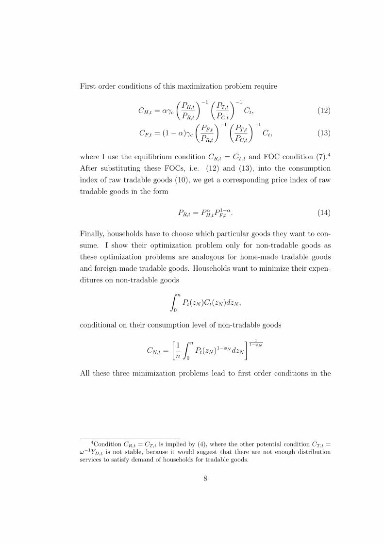
First order conditions of this maximization problem require
CH,t = αγc
(PH,tPR,t
)−1(PT,tPC,t
)−1Ct, (12)
CF,t = (1− α)γc
(PF,tPR,t
)−1(PT,tPC,t
)−1Ct, (13)
where I use the equilibrium condition CR,t = CT,t and FOC condition (7).4
After substituting these FOCs, i.e. (12) and (13), into the consumption
index of raw tradable goods (10), we get a corresponding price index of raw
tradable goods in the form
PR,t = PαH,tP
1−αF,t . (14)
Finally, households have to choose which particular goods they want to con-
sume. I show their optimization problem only for non-tradable goods as
these optimization problems are analogous for home-made tradable goods
and foreign-made tradable goods. Households want to minimize their expen-
ditures on non-tradable goods∫ n
0
Pt(zN)Ct(zN)dzN ,
conditional on their consumption level of non-tradable goods
CN,t =
[1
n
∫ n
0
Pt(zN)1−φNdzN
] 11−φN
All these three minimization problems lead to first order conditions in the
4Condition CR,t = CT,t is implied by (4), where the other potential condition CT,t =ω−1YD,t is not stable, because it would suggest that there are not enough distributionservices to satisfy demand of households for tradable goods.
8

form
Ct(zN) =1
n(1− γc)
(Pt(zN)
PN,t
)−φN (PN,tPC,t
)−1Ct
Ct(zH) =1
nγcα
(Pt(zH)
PH,t
)−φH (PH,tPR,t
)−1(PT,tPC,t
)−1Ct
Ct(zF ) =1
1− nγc(1− α)
(Pt(zF )
PF,t
)−φF (PF,tPR,t
)−1(PT,tPC,t
)−1Ct.
Corresponding price indices are in the form
PN,t =
[1
n
∫ n
0
Pt(zN)1−φNdzN
] 11−φN
PH,t =
[1
n
∫ n
0
Pt(zH)1−φHdzH
] 11−φH
PF,t =
[1
1− n
∫ 1
n
Pt(zF )1−φF dzF
] 11−φF
Similar optimization problems and resulting optimality conditions hold also
for the foreign economy and are distinguished from those in the domestic
economy by superscript ”∗”.
Investment Decisions
Households use part of their income to accumulate capital Kt, assumed to
be homogenous, which they rent to firms. Capital is accumulated according
to the formula
Kt+1 = (1− τ)Kt + εi,t
(1− S
(ItIt−1
))It, (15)
where τ is a depreciation rate of capital and It denotes investment in the
period t. Following Christiano et. al. (2005), capital accumulation is subject
to investment specific technological shock εi,t and adjustment costs repre-
9

sented by function S(·).5 This function has to satisfy following properties
S(1) = S ′(1) = 0 and S ′′(·) = S ′′ > 0.
In order to decide how much capital would a household accumulate, it is
again necessary to solve the optimization problem. Household wants to max-
imize its utility expressed by (1), which is subject to the budget constraint
(2) and to the formula for capital accumulation (15). First order conditions
corresponding to capital Kt and investment It imply the following equations
PI,tPC,t
= εi,t
(1− S
(ItIt−1
)− ItIt−1
S′(
ItIt−1
))QT,t+
+Et
{PC,t+1
PC,tRt
εi,t+1
(It+1
It
)2
S′(It+1
It
)QT,t+1
},
(16)
QT,t = Et
{RK,t+1
PC,t+1
PC,t+1
PC,tRt
}+ (1− τ)Et
{PC,t+1
PC,tRt
QT,t+1
}. (17)
The equation (16) represents the demand for investment and the equation
(17) determines a relative price of installed capital (known as Tobin’s Q)
which is defined as
QT,t =λK,t
λC,tPC,t,
where λC,t is a marginal utility of nominal income (it is also a Lagrange
multiplier on households’ budget constraint) and λK,t is a Lagrange multiplier
on the law of motion for capital.
Homogenous investment goods are produced in a similar way as the final
consumption goods, except that there are no distribution costs associated
5It is not important to know the exact form of this function, because a log-linearisedform of the model contains only a second derivative of the function S′′ (regarded as un-known parameter to be estimated).
10

with using tradable investment goods,6 which implies the following definitions
It =IγiR,tI
1−γiN,t
γγii (1− γi)1−γi,
IR,t =IαH,tI
1−αF,t
αα(1− α)1−α,
PI,t = P γiR,tP
1−γiN,t
It is assumed that a composition of consumption and investment basket in a
given economy can differ, i.e. parameters γc and γi can be different, and that
composition of tradable baskets is identical, i.e. parameter α is the same
for both tradable consumption goods and tradable investment goods in the
given economy.
Wage Setting
Each household is specialized in a different type of labor Lt(j), which it
supplies in a monopolistically competitive labor market. All supplied labor
types are aggregated into homogenous labor input Lt according to the formula
Lt =
[(1
n
) 1φW∫ n
0
Lt(j)φW−1
φW dj
] φWφW−1
,
where φW is the elasticity of substitution between different labor types. A
corresponding aggregate wage index is then defined as
Wt =
[1
n
∫ n
0
Wt(j)1−φW dj
] 11−φW
,
where Wt(j) denotes a wage of the household j. Cost minimization of firms
implies the following demand schedules for each labor type Lt(j) in the form
Lt(j) =1
n
(Wt(j)
Wt
)−θWLt. (18)
6Following Burstein et al. (2003).
11

Following Erceg, Henderson and Levin (2000), a wage setting mechanism
a-la Calvo in a modified version with partial wage indexation is assumed.
According to this set-up, every period only 1 − θW portion of households
(randomly chosen) can reset their wages optimally, while the remaining por-
tion of households θW adjust their wages according to the indexation rule
Wt(j) = Wt−1(j)
(PC,t−1PC,t−2
)δW,
where δW ∈ (0, 1) is a parameter of wage indexation. If I set δW = 0, I get
the original Calvo wage setting mechanism, where all households which can
not reoptimize their wages leave their wages unchanged. By setting δW = 1,
I get the Calvo wage setting mechanism with full wage indexation, where
all households which can not reoptimize their wages fully adjust their wages
according to the past inflation.
Households, which are allowed to reset their wages optimally, want to
maximize their utility represented by the utility function (1), subject to the
set of budget constraints (2) and labor demand constraints (18), taking into
account the Calvo constraint that they can not always reset their wages.
Formally, households want to maximize
Et
∞∑k=0
θkWβk
[− εl,t+k
1 + φLt+k(j)
1+φ + λC,t+kWt(j)
(PC,t+k−1PC,t−1
)δWLt+k(j)
],
which is subject to the following constraint
Lt+k(j) =1
n
[Wt(j)
Wt+k
(PC,t+k−1PC,t−1
)δW]−φWLt+k.
First order condition of this optimization problem is in the form
Et
∞∑k=0
θkWβk
[Wt(j)
PC,t+k
(PC,t+k−1PC,t−1
)δW− φWφW − 1
MRSt+k(j)
]·
· εd,t+k(Ct+k(j)− hCt+k−1)−σLt+k(j) = 0,
12

where φWφW−1
represents gross wage mark-up resulting from certain monopoly
power of the household, MRSt(j) is the marginal rate of substitution between
labor and consumption of household j, defined as
MRSt(j) =εl,tLt(j)
φ
εd,t(Ct(j)− hCt−1)−σ.
Since all households face the same optimization problem, they all set the
same optimal wage Wt. Therefore, the aggregate wage index is then defined
as a weighted average of optimally set wages, and wages which are partially
adjusted according to the past inflation. Formally,
Wt =
θW (Wt−1
(PC,t−1PC,t−2
)δW)1−φW
+ (1− θW )W 1−φWt
11−φW
.
Similar conditions and formulas hold also for the foreign economy. It is
allowed for parameters governing the wage setting of households to differ
between countries.
Firms
Production Technology
There is a continuum of homogenous, monopolistic competitive firms in the
tradable and non-tradable sectors of the domestic economy. The production
functions of firms are represented by Cobb-Douglas functions, homogenous
in labor and capital of degree one (i.e. with constant returns to scale)
Yt(zN) = εaN ,tLt(zN)1−ηKt(zN)η,
Yt(zH) = εaH ,tLt(zH)1−ηKt(zH)η,
where η is the elasticity of output with respect to capital (common to both
sectors, but potentially different in individual countries), and εaH ,t (εaN ,t)
is a productivity shock in the tradable (non-tradable) sector. The index of
13

output in each sector is given by Dixit-Stiglitz aggregator
YN,t =
[(1
n
) 1φN∫ n
0
Yt(zN)φN−1
φN dzN
] φNφN−1
YH,t =
[(1
n
) 1φH∫ n
0
Yt(zH)φH−1
φH dzH
] φHφH−1
.
All firms try to minimize their costs for a given level of production. Formally,
firms try to minimize
minLt(zi)Kt(zi)
WtLt(zi) +RK,tKt(zi) + λi,t(Yt(zi)− εai,tLt(zi)1−ηKt(zi)η), (19)
for i = N,H. Since all firms have the same technology and face the same
prices of inputs, cost minimization (19) requires the same ratio of capital and
labor for all domestic firms
WtLtRK,tKt
=1− ηη
.
Lagrange multiplier λi,t can be interpreted as nominal marginal costs. There-
fore, the real marginal costs, identical for all firms in the given sector, are
defined by the formula
MCi,t =λi,tPi,t
=1
Pi,tεai,t
(Wt
1− η
)1−η (RK,t
η
)η, for i = N,H. (20)
Price Setting
In this section I shall describe price setting problem of firms in the domestic
non-tradable sector. Price setting of foreign firms as well as firms in the
tradable sector is defined analogously.
Firms in the non-tradable sector set their prices in order to maximize
their profits. It is assumed that firms face modified Calvo restriction with
partial indexation on the frequency of price adjustment. According to this
restriction, every period only 1− θN portion of firms in non-tradable sector
14

(randomly chosen) can reset their prices optimally, while θN portion of firms
in non-tradable sector partially adjust their prices according to the past
inflation, following the indexation rule
Pt(zN) = Pt−1(zN)
(PN,t−1PN,t−2
)δN,
where δN is a parameter of price indexation. Setting δN = 0, I get the
original Calvo constraint, as suggested by Calvo (1983). By setting δN = 1,
I get the Calvo constraint with full price indexation, where all firms which
can not reoptimize their prices fully adjust their prices according to the past
inflation.
A firm j, which is allowed to reset its price, chooses the price Pt(zN) in
order to maximize current market value of profits generated until the firm
can again reoptimize its price. Formally, firms solve maximization problem
Et
∞∑k=0
θkNβkλC,t+kYt+k(zN)
[Pt(zN)
(PN,t+k−1PN,t−1
)δN− PN,t+kMCN,t+k
],
taking into account the sequence of demand constraints
Yt+k(zN) =1
n
[Pt(zN)
PN,t+k
(PN,t+k−1PN,t−1
)δN]−φNYN,t+k,
where λC,t is the marginal utility of households’ nominal income in period t,
considered by firms as exogenous, and MCN,t is the real marginal costs in
the period t, defined in (20). The first order condition of the maximization
problem of firms implies
Et
∞∑k=0
θkNβkλC,t+kYt+k(zN)
[Pt(zN)
(PN,t+k−1PN,t−1
)δN−
− φNφN − 1
PN,t+kMCN,t+k
]= 0.
(21)
Firms do not face any firm-specific shocks, so all firms in the given sector
15

choose the same optimal price PN,t. Hence, it is possible to express the
aggregate price index of non-tradable goods as a weighted average of the
optimizing firms’ price PN,t, and the price of firms which adjust their price
to the previous inflation
PN,t =
θN (PN,t−1(PN,t−1PN,t−2
)δN)1−φN
+ (1− θN)P 1−φNN,t
11−φN
. (22)
Foreign firms and domestic firms in the tradable sector deal with analogous
maximization problems. Therefore, first order conditions and resulting price
indices associated with maximization problems of foreign firms and domestic
firms in tradable sector are analogous to those expressed in equations (21)
and (22). It is assumed that structural parameters of price stickiness θ and
price indexation δ as well as stochastic properties of shocks in productivity
can differ among countries and sectors.
It is assumed that prices are set in the producer’s currency and that
international law of one price holds for intermediate tradable goods. Thus,
prices of domestic goods sold in the foreign economy and prices of foreign
goods sold in the domestic economy are given by formulas
P ∗t (zH) = ER−1t Pt(zH) Pt(zF ) = ERtP∗t (zF ),
where ERt is the nominal exchange rate expressed as units of domestic cur-
rency per one unit of foreign currency.
International Risk Sharing
The assumption of complete financial markets implies the perfect risk-sharing
condition. Loosely speaking, this condition requires that prices of similar
bonds must be the same in the domestic as well as in the foreign economy.
16

This condition can be expressed using gross returns on these bonds as
Rt = R∗tEt
{ERt+1
ERt
}.
This formula requires that gross returns on domestic bonds must be the
same as gross returns on foreign bonds adjusted by expected appreciation
(depreciation) of the foreign currency. By substituting for the gross returns
on domestic and foreign bonds from the Euler equation (3) and after subse-
quent mathematical manipulation we get the formula
Qt = κε∗d,tεd,t
(C∗t − h∗C∗t−1)−σ∗
(Ct − hCt−1)−σ, (23)
where
κ = Et
{Qt+1
εd,t+1(Ct+1 − hCt)−σ
ε∗d,t+1(C∗t+1 − h∗C∗t )−σ∗
}is regarded as a constant, which (using iterations) depends on initial condi-
tions and Qt is a real exchange rate defined as
Qt =ERtP
∗C,t
PC,t. (24)
Formula (23) implies that the real exchange rate is proportional to the ratio
of marginal utility of consumption between domestic and foreign households.
The real exchange rate can deviate from purchasing power parity (PPP)
because of changes in relative prices of tradable and non-tradable goods,
changes in relative distribution costs and changes in terms of trade, as long
as there is a difference between household preferences among countries, i.e.
α 6= 1 − α∗. This can be demonstrated this by substituting for the price
indices in the definition of real exchange rate (24) from definitions of these
price indices (8), (9) and (14). After some mathematical manipulation we
obtain
Qt = Sα+α∗−1
t
1 + ω∗D∗t1 + ωDt
X∗1−γ∗ct
X1−γct
,
17

where St are terms of trade defined as domestic import prices relative to
domestic export prices7
St =ERtP
∗F,t
PH,t,
Xt and X∗t are internal exchange rates defined as prices of non-tradable goods
relative to prices of tradable goods
Xt =PN,tPT,t
X∗t =P ∗N,tP ∗T,t
and Dt and D∗t are relative distribution costs, defined as prices of non-
tradable goods relative to prices of raw tradable goods
Dt =PN,tPR,t
D∗t =P ∗N,tP ∗R,t
.
Monetary and Fiscal Authorities
The behavior of central bank is described by a variant of Taylor rule.8
Rt = Rρt−1
[Et
{(Yt+1
Y
)φy ( PC,t+1
(1 + π)PC,t
)φπ}]1−ρεm,t,
where ρ is a parameter of interest rate smoothing, Yt is a total output in the
economy, Y denotes a steady state level of this output, π is a steady state
level of inflation, φy is an elasticity of the interest rate to the output, φπ is
an elasticity of the interest rate to inflation and εm,t is a monetary policy
shock.
Fiscal policy is modeled in a very simple fashion. Government expen-
ditures and transfers to households are fully financed by lump-sum taxes so
7The assumption of law of one price for tradable goods implies S∗t = S−1t .8Here I depart from the original specification of the model. I changed the specification
of the interest rate rules. In the original model, interest rates depend on current inflationand output, while in my specification interest rates depend on expected inflation andexpected output. This, in my view, better corresponds with the actual behavior of centralbanks in both economies.
18

that state budget is balanced every period. Government expenditures consist
only of non-tradable domestic goods and are modeled as a stochastic process
εg,t. Given the assumptions about households, Ricardian equivalence holds
in this model.
Market Clearing Conditions
The model is closed by satisfying the market clearing conditions. Goods
market clearing requires that output of each firm producing non-tradable
goods is either consumed by households in the domestic economy, spent on
investment, used for distribution services or purchased by the government.
Similarly, output of firms producing tradable goods is either consumed or
invested in the domestic or foreign economy. Formally
YN,t = CN,t + IN,t + YD,t +Gt, (25)
YH,t = CH,t + C∗H,t + IH,t + I∗H,t. (26)
By plugging in allocation functions (6), (7), and (12) together with analogous
allocation functions for investment and their foreign counterparts into the
goods market clearing conditions (25) and (26), the aggregate output in both
domestic sectors can be rewritten as
YN,t = (1− γc)(PN,tPC,t
)−1Ct + ωγc
(PT,tPC,t
)−1Ct+
+(1− γi)(PN,tPI,t
)−1It +Gt,
(27)
YH,t = αγc
(PH,tPR,t
)−1(PT,tPC,t
)−1Ct +
1− nn
(1− α∗)γ∗c
(P ∗H,tP ∗R,t
)−1(P ∗T,tP ∗C,t
)−1C∗t
+ αγi
(PH,tPR,t
)−1(PR,tPI,t
)−1It +
1− nn
(1− α∗)γ∗i
(P ∗H,tP ∗R,t
)−1(P ∗R,tP ∗I,t
)−1I∗t ,
19

where in (27) I use the following condition of optimality
YD,t = ωCT,t,
which links distribution services with tradable consumption goods. The total
output in the economy is given by the sum of output in tradable and non-
tradable sectors
Yt = YN,t + YH,t.
Finally, market clearing conditions for factor markets requires
Lt =
∫ n
0
Lt(zN)dzN +
∫ n
0
Lt(zH)dzH
Kt =
∫ n
0
Kt(zN)dzN +
∫ n
0
Kt(zH)dzH .
Analogous market clearing conditions hold for the foreign economy, too.
Exogenous Shocks
Behavior of the model is driven by seven structural shocks in each economy:
productivity shocks in tradable sector (εaH ,t and ε∗aF ,t), productivity shocks
in non-tradable sector (εaN ,t and ε∗aN ,t), labor supply shocks (εl,t and ε∗l,t),
investment efficiency shocks (εi,t and ε∗i,t), consumption preference shocks
(εd,t and ε∗d,t), government spending shocks (εg,t and ε∗g,t) and monetary policy
shocks (εm,t and ε∗m,t). Except for monetary policy shocks, all other shocks
are represented by AR1 processes in the log-linearised version of the model,
see (68) - (79). Monetary policy shocks are represented by IID processes in
the log-linearised version of the model.9 I also allow for correlations between
innovations in corresponding domestic and foreign shocks.
9IID - identically and independently distributed
20

Log-linearised Model
The model presented above is highly non-linear and does not have any ana-
lytical solution. A log-linear approximation around the non-stochastic steady
state is employed for the purposes of empirical analysis. For details about
methods of log-linear approximation see Uhlig (1995). Nice introduction to
methods used for log-linearising around the steady state is provided by Zi-
etz (2006). In this section I present a log-linearised form of the model. All
variables of the model are in the form of log-deviations from their respective
steady state. Formally, xt = logXt− logX, where X is a steady state value.
The model is formed by 40 equations describing endogenous variables
(from equation (28) to equation (67)) and by 12 equations for exogenous
shocks (from equation (68) to equation (79)). An interpretation of the model
variables is presented in Table 1. Interpretation of the structural parameters
and the parameters related to shocks is presented in Tables 2 and 3.
Market Clearing Conditions:
yH,t =C
Y H
γcα
1 + ω(ct + (1− γc)xt + (1− α)st)
+C∗
Y H
1− nn
γ∗c (1− α∗)1 + ω∗
(c∗t + (1− γ∗c )x∗t + α∗st)
+I
Y H
γiα (it + (1− γi)(1 + ω)xt + (1− α)st)
+I∗
Y H
1− nn
γ∗i (1− α∗) (i∗t + (1− γ∗i )(1 + ω)x∗t + α∗st)
(28)
21

y∗F,t =C∗
Y∗F
γ∗cα∗
1 + ω∗(c∗t + (1− γ∗c )x∗t − (1− α∗)st)
+C
Y∗F
n
1− nγc(1− α)
1 + ω(ct + (1− γc)xt − αst)
+I∗
Y∗F
γ∗i α∗ (i∗t + (1− γ∗i )(1 + ω∗)x∗t − (1− α∗)st)
+I
Y∗F
n
1− nγi(1− α) (it + (1− γi)(1 + ω)xt − αst)
(29)
yN,t =C
Y N
((1− γc)(ct − γcxt) +
γcω
1 + ω(ct + (1− γc)xt)
)+
I
Y N
(1− γi)(it − γi(1 + ω)xt) +G
Y N
εg,t
(30)
y∗N,t =C∗
Y∗N
((1− γ∗c )(c∗t − γ∗cx∗t ) +
γ∗cω∗
1 + ω∗(c∗t + (1− γ∗c )x∗t )
)+
I∗
Y∗N
(1− γ∗i )(i∗t − γ∗i (1 + ω∗)x∗t ) +G∗
Y∗N
ε∗g,t
(31)
yt =Y H
YyH,t +
Y N
YyN,t (32)
y∗t =Y∗F
Y∗ y∗F,t +
Y∗N
Y∗ y∗N,t (33)
Euler Equation:
ct − hct−1 = Et(ct+1 − hct)−1− hσ
Et (rt − πt+1 + εd,t+1 − εd,t) (34)
c∗t − h∗c∗t−1 = Et(c∗t+1 − h∗c∗t )−
1− h∗
σ∗Et(r∗t − π∗t+1 + ε∗d,t+1 − ε∗d,t
)(35)
International Risk Sharing Condition:
qt = ε∗d,t − εd,t −σ∗
1− h∗(c∗t − h∗c∗t−1) +
σ
1− h(ct − hct−1) (36)
22
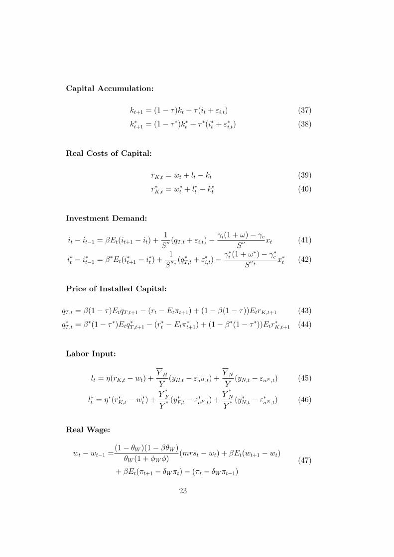
Capital Accumulation:
kt+1 = (1− τ)kt + τ(it + εi,t) (37)
k∗t+1 = (1− τ ∗)k∗t + τ ∗(i∗t + ε∗i,t) (38)
Real Costs of Capital:
rK,t = wt + lt − kt (39)
r∗K,t = w∗t + l∗t − k∗t (40)
Investment Demand:
it − it−1 = βEt(it+1 − it) +1
S ′′(qT,t + εi,t)−
γi(1 + ω)− γcS ′′
xt (41)
i∗t − i∗t−1 = β∗Et(i∗t+1 − i∗t ) +
1
S ′′∗(q∗T,t + ε∗i,t)−
γ∗i (1 + ω∗)− γ∗cS ′′∗
x∗t (42)
Price of Installed Capital:
qT,t = β(1− τ)EtqT,t+1 − (rt − Etπt+1) + (1− β(1− τ))EtrK,t+1 (43)
q∗T,t = β∗(1− τ ∗)Etq∗T,t+1 − (r∗t − Etπ∗t+1) + (1− β∗(1− τ ∗))Etr∗K,t+1 (44)
Labor Input:
lt = η(rK,t − wt) +Y H
Y(yH,t − εaH ,t) +
Y N
Y(yN,t − εaN ,t) (45)
l∗t = η∗(r∗K,t − w∗t ) +Y∗F
Y∗ (y∗F,t − ε∗aF ,t) +
Y∗N
Y∗ (y∗N,t − ε∗aN ,t) (46)
Real Wage:
wt − wt−1 =(1− θW )(1− βθW )
θW (1 + φWφ)(mrst − wt) + βEt(wt+1 − wt)
+ βEt(πt+1 − δWπt)− (πt − δWπt−1)(47)
23

w∗t − w∗t−1 =(1− θ∗W )(1− β∗θ∗W )
θ∗W (1 + φ∗Wφ∗)
(mrs∗t − w∗t ) + β∗Et(w∗t+1 − w∗t )
+ β∗Et(π∗t+1 − δ∗Wπ∗t )− (π∗t − δ∗Wπ∗t−1)
(48)
Marginal Rate of Substitution:
mrst = εl,t + φlt − εd,t +σ
1− h(ct − hct−1) (49)
mrs∗t = ε∗l,t + φ∗l∗t − ε∗d,t +σ∗
1− h∗(c∗t − h∗c∗t−1) (50)
Phillips Curve for Tradable Sector:
πH,t − δHπH,t−1 = βEt(πH,t+1 − δHπH,t) +(1− θH)(1− βθH)
θHmcH,t (51)
π∗F,t − δ∗Fπ∗F,t−1 = β∗Et(π∗F,t+1 − δ∗Fπ∗F,t) +
(1− θ∗F )(1− β∗θ∗F )
θ∗Fmc∗F,t (52)
Phillips Curve for Non-tradable Sector:
πN,t − δNπN,t−1 = βEt(πN,t+1 − δNπN,t) +(1− θN)(1− βθN)
θNmcN,t (53)
π∗N,t − δ∗Nπ∗N,t−1 = β∗Et(π∗N,t+1 − δ∗Nπ∗N,t)+
+(1− θ∗N)(1− β∗θ∗N)
θ∗Nmc∗N,t
(54)
Real Marginal Costs in Tradable Sector:
mcH,t = (1− η)wt + ηrK,t − εaH ,t + (1− α)st + (1− γc + ω)xt (55)
mc∗F,t = (1− η∗)w∗t + η∗r∗K,t − ε∗aF ,t + (1− α∗)st + (1− γ∗c + ω∗)x∗t (56)
Real Marginal Costs in Non-tradable Sector:
mcN,t = (1− η)wt + ηrK,t − εaN ,t − γcxt (57)
mc∗N,t = (1− η∗)w∗t + η∗r∗K,t − ε∗aN ,t − γ∗cx∗t (58)
24

Relative Price of Non-tradable Goods:
xt − xt−1 = πN,t − πT,t (59)
x∗t − x∗t−1 = π∗N,t − π∗T,t (60)
Inflation of Tradable Goods:
πT,t =1
1 + ω(πH,t + (1− α)∆st + ωπN,t) (61)
π∗T,t =1
1 + ω∗(π∗F,t + (1− α∗)∆st + ω∗π∗N,t
)(62)
Overall Inflation:
πt = γcπT,t + (1− γc)πN,t (63)
π∗t = γ∗cπ∗T,t + (1− γ∗c )π∗N,t (64)
Real Exchange Rate:
qt = (α + α∗ − 1)st + (1− γ∗c + ω∗)x∗t − (1− γc + ω)xt (65)
Monetary Policy Rule:
rt = ρrt−1 + (1− ρ)(ψyEt{yt+1}+ ψπEt{πt+1}) + εm,t (66)
r∗t = ρ∗r∗t−1 + (1− ρ∗)(ψ∗yEt{y∗t+1}+ ψ∗πEt{π∗t+1}) + ε∗m,t (67)
Productivity Shock in Tradable Sector:
εaH ,t = ρaHεaH ,t−1 + µaH ,t (68)
ε∗aF ,t = ρ∗aF ε∗aF ,t−1 + µ∗aF ,t (69)
Productivity Shock in Non-tradable Sector:
εaN ,t = ρaNεaN ,t−1 + µaN ,t (70)
ε∗aN ,t = ρ∗aNε∗aN ,t−1 + µ∗aN ,t (71)
25

Preference Shock:
εd,t = ρdεd,t−1 + µd,t (72)
ε∗d,t = ρ∗dε∗d,t−1 + µ∗d,t (73)
Labor Supply Shock:
εl,t = ρlεl,t−1 + µl,t (74)
ε∗l,t = ρ∗l ε∗l,t−1 + µ∗l,t (75)
Shock in Government Expenditures:
εg,t = ρgεg,t−1 + µg,t (76)
ε∗g,t = ρ∗gε∗g,t−1 + µ∗g,t (77)
Shock in Investment Efficiency:
εi,t = ρiεi,t−1 + µi,t (78)
ε∗i,t = ρ∗i ε∗i,t−1 + µ∗i,t (79)
26

Table 1: Interpretation of Variablesvariable interpretation
ct,c∗t consumption
it,i∗t investment
yt,y∗t total output
yH,t,y∗F,t output in tradable sector
yN,t,y∗N,t output in non-tradable sector
xt,x∗t internal exchange rates
st terms of tradert,r
∗t nominal interest rate
qt real exchange ratekt,k
∗t capital
rK,t,r∗K,t payoff from renting capital
wt,w∗t real wage
qT,t,q∗T,t price of installed capital (Tobin’s Q)
lt,l∗t labor
mrst,mrs∗t marginal rate of substitution
πt,π∗t inflation
πT,t,π∗T,t inflation of tradable goods
πH,t,π∗F,t inflation in tradable sector
πN,t,π∗N,t inflation of non-tradable goods
mcH,t,mc∗F,t real marginal costs in tradable sector
mcN,t,mc∗N,t real marginal costs in non-tradable sector
εaH ,t,ε∗aF ,t productivity shock in tradable sector
εaN ,t,ε∗aN ,t productivity shock in non-tradable sector
εd,t,ε∗d,t preference shock
εl,t,ε∗l,t labor supply shock
εg,t,ε∗g,t government expenditures shock
εi,t,ε∗i,t investment efficiency shock
εm,t,ε∗m,t monetary policy shock
27

Table 2: Interpretation of Structural Parametersparameter interpretation domain
n relative size of the domestic economy 〈0, 1〉β, β∗ discount factor 〈0, 1〉h, h∗ habit formation in consumption 〈0, 1〉σ, σ∗ inv. elast. of intertemporal substitution 〈0,∞)φ, φ∗ inv. elast. of labor supply 〈0,∞)φH , φF elast. of subst. among tradable goods 〈1,∞)φN , φ∗N elast. of subst. among non-tradable goods 〈1,∞)φW , φ∗W elast. of subst. among labor types 〈1,∞)γc, γ
∗c share of tradable goods in consumption 〈0, 1〉
γi, γ∗i share of tradable goods in investment 〈0, 1〉
α, α∗ share of domestic tradable goods 〈0, 1〉ω, ω∗ distribution costs 〈0,∞)τ , τ ∗ capital depreciation rate 〈0, 1〉S′′, S′′∗ adjustment costs of capital 〈0,∞)
η, η∗ elasticity of output with respect to capital 〈0, 1〉θH , θ
∗F Calvo parameter for tradable sector 〈0, 1〉
θN , θ∗N Calvo parameter for non-tradable sector 〈0, 1〉
θW , θ∗W Calvo parameter for households 〈0, 1〉
δH , δ∗F indexation in tradable sector 〈0, 1〉
δN , δ∗N indexation in non-tradable sector 〈0, 1〉
δW , δ∗W indexation of households 〈0, 1〉
ρi, ρ∗i interest rate smoothing 〈0, 1〉
ψπ, ψ∗π elasticity of interest rate to inflation 〈0,∞)
ψy, ψ∗y elasticity of interest rate to output 〈0,∞)
28
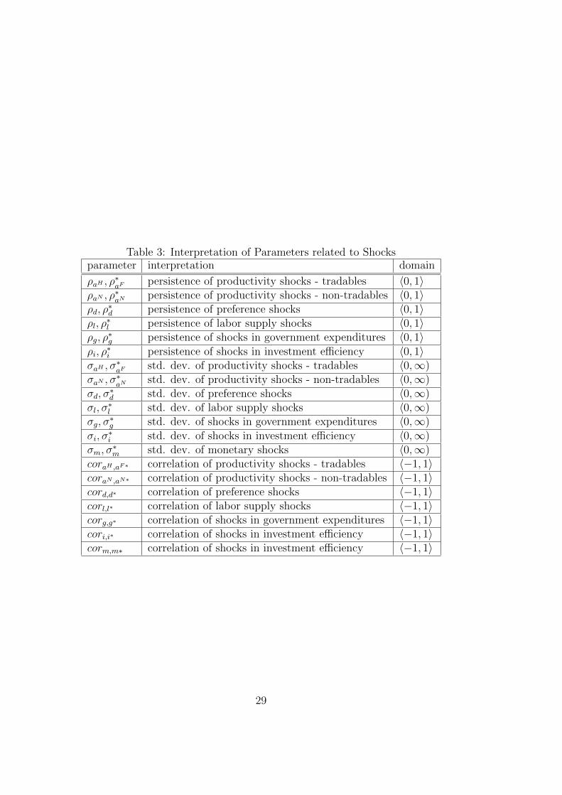
Table 3: Interpretation of Parameters related to Shocksparameter interpretation domain
ρaH , ρ∗aF persistence of productivity shocks - tradables 〈0, 1〉
ρaN , ρ∗aN persistence of productivity shocks - non-tradables 〈0, 1〉
ρd, ρ∗d persistence of preference shocks 〈0, 1〉
ρl, ρ∗l persistence of labor supply shocks 〈0, 1〉
ρg, ρ∗g persistence of shocks in government expenditures 〈0, 1〉
ρi, ρ∗i persistence of shocks in investment efficiency 〈0, 1〉
σaH , σ∗aF std. dev. of productivity shocks - tradables 〈0,∞)
σaN , σ∗aN std. dev. of productivity shocks - non-tradables 〈0,∞)
σd, σ∗d std. dev. of preference shocks 〈0,∞)
σl, σ∗l std. dev. of labor supply shocks 〈0,∞)
σg, σ∗g std. dev. of shocks in government expenditures 〈0,∞)
σi, σ∗i std. dev. of shocks in investment efficiency 〈0,∞)
σm, σ∗m std. dev. of monetary shocks 〈0,∞)
coraH ,aF∗ correlation of productivity shocks - tradables 〈−1, 1〉coraN ,aN∗ correlation of productivity shocks - non-tradables 〈−1, 1〉cord,d∗ correlation of preference shocks 〈−1, 1〉corl,l∗ correlation of labor supply shocks 〈−1, 1〉corg,g∗ correlation of shocks in government expenditures 〈−1, 1〉cori,i∗ correlation of shocks in investment efficiency 〈−1, 1〉corm,m∗ correlation of shocks in investment efficiency 〈−1, 1〉
29

References
[1] Burstein AT, Neves JC, Rebelo S (2003): Distribution Costs and Real
Exchange Rate Dynamics during Exchange-rate-based Stabilizations.
Journal of Monetary Economics, 50(6):1189-1214.
[2] Calvo G (1983): Staggered Prices in a Utility-maximizing Framework.
Journal of Monetary Economics, 12(3):383-398.
[3] Christiano L, Eichenbaum M, Evans C (2005): Nominal Rigidities and
the Dynamic Effects of a Shock to Monetary Policy. Journal of Political
Economy, 113(1):1-45.
[4] Corsetti G, Dedola L (2005): A Macroeconomic Model of International
Price Discrimination. Journal of International Economics, 67(1): 129-
155.
[5] Erceg CJ, Henderson DW, Levin AT (2000): Optimal Monetary Policy
with Staggered Wage and Price Contracts. Journal of Monetary Eco-
nomics, 46(2):281-313.
[6] Herber P (2010): Strukturalnı odlisnosti ceske ekonomiky a ekonomiky
Evropske unie z pohledu DSGE modelu. Masaryk University, Master
Thesis.
[7] Herber P, Nemec D (2012): Investigating Structural Differences of the
Czech Economy: Does Asymmetry of Shocks Matter? Bulletin of the
Czech Econometric Society, 19(29):28-49.
30
[8] Kolasa M (2009): Structural Heterogeneity or Asymmetric Shocks?
Poland and the Euro Area through the Lens of a Two-country DSGE
Model. Economic Modelling, 26(6):1245-1269.
[9] Uhlig H (1995): A Toolkit for Analyzing Nonlinear Dynamic Stochas-
tic Models Easily. Discussion Paper, Institute for Empirical Macroeco-
nomics 101, Federal Reserve Bank of Minneapolis.
[10] Zietz J (2006): Log-Linearizing Around the Steady State: A
Guide with Examples. Working Paper Series, Available at SSRN:
http://ssrn.com/abstract=951753.
31

Appendix - Software
Dynare
The model is estimated using the programme Dynare, version 4.2.4. It is a
free toolbox for Matlab and it was designed for solving and estimating a wide
class of economic models, especially those with rational expectations. It is a
very suitable tool for handling DSGE models. Dynare offers two approaches
to the estimation of the model: (i) maximal likelihood method and (ii) Ran-
dom Walk Chain Metropolis-Hastings algorithm. Beside the estimation, it is
also able to produce many useful statistics, such as convergence diagnostics
of the MH algorithm, checkplots, impulse-response functions, variance de-
composition, shock decomposition, conditional and unconditional forecasts,
etc. All versions of Dynare toolbox and Dynare manuals are available on the
website http://www.dynare.org/.
IRIS
Several exercises which are presented in Appendix, namely (i) comparison of
second moments implied by the data and the model; and (ii) comparison of
the model predictions with the actual observations; were performed by the
programme IRIS developed by Jaromır Benes.10 IRIS is a free toolbox for
Matlab designed for solving, estimating and evaluating the dynamic economic
models. It is a very suitable tool for handling conditional and unconditional
forecasts and for comparison of second moments (model vs. data). Unlike
10IRIS is an acronym of ”I Rest, Iris Solves”.
32
Dynare, it is also able to produce impulse-responses to anticipated shocks.
All versions of IRIS toolbox as well as IRIS manuals are available on the
website http://code.google.com/p/iris-toolbox-project/
Demetra
Seasonal adjustment of the data was performed in the Demetra programme.
Demetra is a free software designed for seasonal adjustment of time series,
developed by researchers from Eurostat and the National Bank of Belgium.
Demetra offers several specifications of TRAMO/SEATS and X12 methods
for seasonal adjustment of time series. It also performs many statistical tests
focusing on evaluation of the quality of seasonal adjustment. All versions
of the programme Demetra as well as various manuals and guidelines are
available on http://www.cros-portal.eu/page/demetra
33

Appendix - Data
Real GDP, consumption and investment are measured as ”Millions of euro,
chain-linked volumes, reference year 2005 (at 2005 exchange rates)”. Con-
sumption is given by ”Household and NPISH final consumption expendi-
tures”.11 Investment is given by ”Gross fixed capital formation”.
Prices are measured by the ”HICP, Index, 2005=100, All-items HICP”.
Real wage is given by the ”Labour Cost Index - Wages and salaries, Nominal
value, Business economy, Index, 2008=100, Data adjusted by working days”,
which is divided by HICP in each period. Short-term interest rate is given
by the ”Money market interest rates, 3-month rates”.
Internal exchange rate defined as prices of non-tradable goods relative to
prices of tradable goods is calculated from the components of HICP, where
”Services (overall index excluding goods)” and ”Energy” are regarded as non-
tradable goods, while ”Non-energy industrial goods” and ”Food including
alcohol and tobacco” are regarded as tradable goods.
Except for the nominal interest rates, all observed variables are season-
ally adjusted. I used TRAMO/SEATS algorithm for seasonal adjustment of
the time series and took advantage of the Demetra software developed for
seasonal adjustment of time series.12 Although many time series are also
available as seasonally adjusted on Eurostat, I decided to download all previ-
11The data series labeled as ”Final consumption expenditures of households” are notavailable for the Euro Area 12, which is why I use ”Household and NPISH final consump-tion expenditures”. However, values of ”Final consumption expenditure of NPISH” are sonegligible that it does not make make any significant difference.
12The best performance from the available variants of TRAMO/SEATS algorithm wasmade by specification ”Tramo-Seats RSA2 log/level, working days, Easter, outliers detec-tion, airline model”, which is what I decided to use for seasonal adjustment of employedtime series.
34

ously mentioned time series as not seasonally adjusted and then adjust them
myself. There are several reasons for this decision. First, the seasonally ad-
justed versions of HICP and its components are unavailable. I find it more
consistent to use time series all of which are adjusted by the same method
than use time series adjusted by possibly different methods. Secondly, some
of those time series which are available as seasonally adjusted on Eurostat
clearly show some residual seasonality (also detected by Demetra), which
raises doubts about quality of the employed seasonal adjustment.
Except for the nominal interest rates, all observed variables are expressed
as demeaned 100*log differences. Nominal interest rates are demeaned and
expressed as quarterly rates per cent. The following formulas show how are
transformed observed variables linked to the model variables.
CZ: EA:
consumption: Cobst = ct − ct−1 Cobs∗
t = c∗t − c∗t−1investment: Iobst = it − it−1 Iobs∗t = i∗t − i∗t−1GDP: Y obs
t = yt − yt−1 Y obs∗t = y∗t − y∗t−1
prices: HICP obst = πt HICP obs∗
t = π∗t
int. exchange rate: Xobst = xt − xt−1 Xobs∗
t = x∗t − x∗t−1real wage: W obs
t = wt − wt−1 W obs∗t = w∗t − w∗t−1
interest rate: Robst = rt Robs∗
t = r∗t
Figure 1 displays original and seasonally adjusted data, both transformed
as log differences. It shows the performance of the employed seasonal adjust-
ment and also demonstrates how important is correct seasonal adjustment of
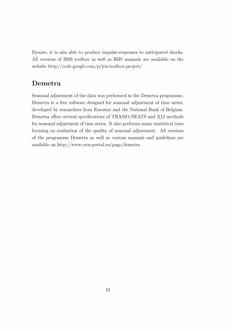
time series. Figure 2 displays transformed data which enter the estimation.
35

Figure 1: Original Data (green line) and Seasonally Adjusted Data (blueline) - Log Differences
2000 2002 2004 2006 2008 2010 2012−10
0
10consumption CZ − 100*log differences
2000 2002 2004 2006 2008 2010 2012−5
0
5consumption EA12 − 100*log differences
2000 2002 2004 2006 2008 2010 2012−50
0
50investment CZ − 100*log differences
2000 2002 2004 2006 2008 2010 2012−20
0
20investment EA12 − 100*log differences
2000 2002 2004 2006 2008 2010 2012−20
0
20GDP CZ − 100*log differences
2000 2002 2004 2006 2008 2010 2012−10
0
10GDP EA12 − 100*log differences
2000 2002 2004 2006 2008 2010 2012−20
0
20real wage CZ − 100*log differences
2000 2002 2004 2006 2008 2010 2012−20
0
20real wage EA12 − 100*log differences
2000 2002 2004 2006 2008 2010 2012−5
0
5HICP CZ − 100*log differences
2000 2002 2004 2006 2008 2010 2012−2
0
2HICP EA12 − 100*log differences
2000 2002 2004 2006 2008 2010 2012−5
0
5int. exchange rate CZ − 100*log differences
2000 2002 2004 2006 2008 2010 2012−5
0
5int. exchange rate EA12 − 100*log differences
36
Figure 2: Data for Estimation
2000 2002 2004 2006 2008 2010 2012−2
0
2consumption CZ − demeaned 100*log differences
2000 2002 2004 2006 2008 2010 2012−1
0
1consumption EA12 − demeaned 100*log differences
2000 2002 2004 2006 2008 2010 2012−10
0
10investment CZ − demeaned 100*log differences
2000 2002 2004 2006 2008 2010 2012−10
0
10investment EA12 − demeaned 100*log differences
2000 2002 2004 2006 2008 2010 2012−5
0
5GDP CZ − demeaned 100*log differences
2000 2002 2004 2006 2008 2010 2012−5
0
5GDP EA12 − demeaned 100*log differences
2000 2002 2004 2006 2008 2010 2012−5
0
5real wage CZ − demeaned 100*log differences
2000 2002 2004 2006 2008 2010 2012−5
0
5real wage EA12 − demeaned 100*log differences
2000 2002 2004 2006 2008 2010 2012−2
0
2HICP CZ − demeaned 100*log differences
2000 2002 2004 2006 2008 2010 2012−2
0
2HICP EA12 − demeaned 100*log differences
2000 2002 2004 2006 2008 2010 2012−5
0
5int. exchange rate CZ − demeaned 100*log differences
2000 2002 2004 2006 2008 2010 2012−5
0
5int. exchange rate EA12 − demeaned 100*log differences
2000 2002 2004 2006 2008 2010 2012−1
0
1interest rate CZ − demeaned quarterly rate
2000 2002 2004 2006 2008 2010 2012−1
0
1interest rate EA12 − demeaned quarterly rate
37
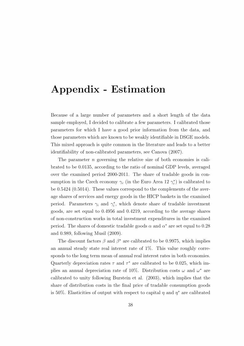
Appendix - Estimation
Because of a large number of parameters and a short length of the data
sample employed, I decided to calibrate a few parameters. I calibrated those
parameters for which I have a good prior information from the data, and
those parameters which are known to be weakly identifiable in DSGE models.
This mixed approach is quite common in the literature and leads to a better
identifiability of non-calibrated parameters, see Canova (2007).
The parameter n governing the relative size of both economies is cali-
brated to be 0.0135, according to the ratio of nominal GDP levels, averaged
over the examined period 2000-2011. The share of tradable goods in con-
sumption in the Czech economy γc (in the Euro Area 12 γ∗c ) is calibrated to
be 0.5424 (0.5014). These values correspond to the complements of the aver-
age shares of services and energy goods in the HICP baskets in the examined
period. Parameters γi and γ∗i , which denote share of tradable investment
goods, are set equal to 0.4956 and 0.4219, according to the average shares
of non-construction works in total investment expenditures in the examined
period. The shares of domestic tradable goods α and α∗ are set equal to 0.28
and 0.989, following Musil (2009).
The discount factors β and β∗ are calibrated to be 0.9975, which implies
an annual steady state real interest rate of 1%. This value roughly corre-
sponds to the long term mean of annual real interest rates in both economies.
Quarterly depreciation rates τ and τ ∗ are calibrated to be 0.025, which im-
plies an annual depreciation rate of 10%. Distribution costs ω and ω∗ are
calibrated to unity following Burstein et al. (2003), which implies that the
share of distribution costs in the final price of tradable consumption goods
is 50%. Elasticities of output with respect to capital η and η∗ are calibrated
38

at 0.3868 and 0.3654, which corresponds to the complement to the average
shares of labor on the GDP in the given economy in the period 2000-2010.13
Elasticities of substitution among labor types φW and φ∗W , which are known
to be badly identifiable, are set equal to 3 following Smets and Wouters
(2003). This value implies a wage mark-up of 50%. Following Slanicay and
Vasıcek (2009, 2011), Capek (2010) and Matheson (2010), who argue that
incorporating price (wage) indexation into the Calvo price (wage) setting
mechanism deteriorates the empirical fit of DSGE models, I decided to set
indexation parameters δH , δ∗F , δN , δ∗N , δW and δ∗W equal to 0. It implies that
the estimated variant of the model employs the original Calvo price (wage)
setting mechanism, see Calvo (1983).
Steady state shares of consumption, investment and government spending
in the total output correspond to their average shares in the GDP in the
examined period. Namely, CY
= 0.4946, IY
= 0.2620, C∗
Y ∗= 0.5691 and
I∗
Y ∗= 0.2036. Other steady state shares are calculated consistently with the
derivation of the model (analogously for the foreign economy):
G
Y= 1− C
Y− I
Y,
YN
Y=
1 + ω − γc1 + ω
C
Y+ (1− γi)
I
Y+G
Y,
YH
Y= 1− YN
Y.
Remaining parameters are estimated. Prior setting of the estimated pa-
rameters is presented in Table 4. For parameters whose natural domain is the
interval between 0 and 1, I chose Beta distribution of priors. For structural
parameters whose natural domain is the set of non-negative real numbers, I
chose Gamma distribution of priors, except for the parameters of adjustment
costs S′′, S′′∗. For those I chose Normal distribution of priors. For parameters
representing standard deviations of shocks, whose natural domain is the set
of non-negative real numbers, I chose Inverse Gamma distribution of priors.
13See http://stats.oecd.org.
39

Finally, for parameters representing correlations between shocks, whose nat-
ural domain is the interval between −1 and 1, I chose Normal distribution
of priors, with the obvious restriction.
Prior means for Calvo parameters of price and wage stickiness θH , θ∗F , θN ,
θ∗N , θW , and θ∗W are set to be 0.7 which implies average price (wage) duration
of 10 months. Priors for parameters in the Taylor rule are set consistently
with Taylor (1999). Inverse elasticities of intertemporal substitution σ and
σ∗ and inverse Frisch elasticities of labor supply φ φ∗ are estimated with
relatively loose priors with prior means set to be 1.0, following Galı (2008),
and prior std. deviations equal to 0.7, which are values commonly found in
the business cycle literature. Parameters of habit formation h and h∗ are
estimated with prior means set to be 0.7 and prior std. deviations equal to
0.1, as in Smets and Wouters (2003). Priors for capital adjustment costs
S′′
and S′′∗ are taken from Kolasa (2009). Priors for shocks are taken from
Herber (2010).
40

Table 4: Priors for Estimated Prametersparameter prior mean prior std. dev. distribution
h, h∗ 0.7 0.1 Betaσ, σ∗ 1.0 0.7 Gammaφ, φ∗ 1.0 0.7 Gamma
S′′, S′′∗ 4.0 1.5 Normal
θH , θ∗F 0.7 0.05 Beta
θN , θ∗N 0.7 0.05 Beta
θW , θ∗W 0.7 0.05 Beta
ρ, ρ∗ 0.7 0.15 Betaψπ, ψ
∗π 1.3 0.15 Gamma
ψy, ψ∗y 0.25 0.1 Gamma
ρaH , ρ∗aF 0.7 0.1 Beta
ρaN , ρ∗aN 0.7 0.1 Beta
ρd, ρ∗d 0.7 0.1 Beta
ρl, ρ∗l 0.7 0.1 Beta
ρg, ρ∗g 0.7 0.1 Beta
ρi, ρ∗i 0.7 0.1 Beta
σaH , σ∗aF 2 ∞ Inv. Gamma
σaN , σ∗aN 2 ∞ Inv. Gamma
σd, σ∗d 6 ∞ Inv. Gamma
σl, σ∗l 10 ∞ Inv. Gamma
σg, σ∗g 3 ∞ Inv. Gamma
σi, σ∗i 6 ∞ Inv. Gamma
σm, σ∗m 0.3 ∞ Inv. Gamma
coraH ,aF∗ 0 0.4 NormalcoraN ,aN∗ 0 0.4 Normalcord,d∗ 0 0.4 Normalcorl,l∗ 0 0.4 Normalcorg,g∗ 0 0.4 Normalcori,i∗ 0 0.4 Normalcorm,m∗ 0 0.4 Normal
41

Table 5: Estimated Valuesparameter posterior 90% credible posterior 90% credible
mean CZ CZ mean EA EA
h, h∗ 0.78 0.68 0.89 0.81 0.72 0.90σ, σ∗ 2.03 0.92 3.09 3.39 1.69 4.99φ, φ∗ 0.52 0.04 1.00 0.91 0.16 1.64
S′′, S′′∗ 6.01 4.21 7.83 5.26 3.38 7.06
θH , θ∗F 0.72 0.64 0.79 0.7 0.64 0.76
θN , θ∗N 0.76 0.70 0.81 0.68 0.62 0.74
θW , θ∗W 0.75 0.69 0.82 0.78 0.72 0.84
ρ, ρ∗ 0.9 0.88 0.93 0.88 0.85 0.91ψπ, ψ
∗π 1.22 1.02 1.4 1.41 1.17 1.65
ψy, ψ∗y 0.12 0.07 0.17 0.27 0.16 0.38
ρaH , ρ∗aF 0.95 0.92 0.98 0.68 0.55 0.81
ρaN , ρ∗aN 0.46 0.33 0.58 0.66 0.56 0.76
ρd, ρ∗d 0.82 0.72 0.91 0.69 0.58 0.81
ρl, ρ∗l 0.49 0.35 0.62 0.49 0.35 0.63
ρg, ρ∗g 0.85 0.79 0.92 0.73 0.64 0.83
ρi, ρ∗i 0.79 0.72 0.87 0.76 0.67 0.84
σaH , σ∗aF 6.01 3.45 8.51 4.75 2.87 6.54
σaN , σ∗aN 6.84 3.55 10.02 2.59 1.60 3.54
σd, σ∗d 5.24 2.74 7.63 5.05 2.85 7.15
σl, σ∗l 32.8 8.57 57.88 25.53 7.07 43.29
σg, σ∗g 3.29 2.61 3.95 1.52 1.26 1.77
σi, σ∗i 4.39 3.09 5.65 4.24 2.93 5.49
σm, σ∗m 0.08 0.07 0.10 0.09 0.08 0.11
coraH ,aF∗ -0.26 -0.47 -0.04coraN ,aN∗ 0.27 0.05 0.48cord,d∗ 0.45 0.25 0.66corl,l∗ -0.17 -0.40 0.06corg,g∗ 0.35 0.15 0.56cori,i∗ 0.33 0.13 0.54corm,m∗ 0.57 0.39 0.76
42

References
[1] Burstein AT, Neves JC, Rebelo S (2003): Distribution Costs and Real
Exchange Rate Dynamics during Exchange-rate-based Stabilizations.
Journal of Monetary Economics, 50(6):1189-1214.
[2] Calvo G (1983): Staggered Prices in a Utility-maximizing Framework.
Journal of Monetary Economics, 12(3):383-398.
[3] Canova F (2007): Methods for Applied Macroeconomic Research. Prince-
ton University Press, Princeton.
[4] Capek J (2010): Comparing the fit of New Keynesian DSGE mod-
els. Ekonomicka revue - Central European Review of Economic Issues,
13(4):207-218.
[5] Galı J (2008): Monetary Policy, Inflation, and the Business Cycle: An
Introduction to the New Keynesian Framework. Princeton University
Press, Princeton.
[6] Herber P (2010): Strukturalnı odlisnosti ceske ekonomiky a ekonomiky
Evropske unie z pohledu DSGE modelu. Masaryk University, Master
Thesis.
[7] Kolasa M (2009): Structural Heterogeneity or Asymmetric Shocks?
Poland and the Euro Area through the Lens of a Two-country DSGE
Model. Economic Modelling, 26(6):1245-1269.
[8] Matheson TD (2010): Assessing the Fit of Small Open Economy DSGEs.
Journal of Macroeconomics, 32(3):906-920.
43
[9] Musil K (2009): International Growth Rule Model: New Approach to
the Foreign Sector of the Open Economy. Masaryk University, PhD The-
sis.
[10] Slanicay M, Vasıcek O (2009): Porovnanı ruznych specifikacı novokey-
nesianskeho DSGE modelu male otevrene ekonomiky pro CR. In: Slany
A (ed): Ekonomicke prostredı a konkurenceschopnost. Masarykova uni-
verzita, Brno, 203-216.
[11] Slanicay M, Vasıcek O (2011): Habit Formation, Price Indexation and
Wage Indexation in the DSGE Model: Specification, Estimation and
Model Fit. Narodohospodarsky obzor - Review of Economic Perspectives,
11(2):71-92.
[12] Smets F, Wouters R (2003): An Estimated Dynamic Stochastic General
Equilibrium Model of the Euro Area. Journal of the European Economic
Association, 1(5):1123-1175.
[13] Taylor JB (1999): A Historical Analysis of Monetary Policy Rules. In:
Taylor JB (ed): Monetary Policy Rules. University of Chicago Press,
Chicago, 319 - 348.
44

Appendix - MCMC
Convergence Diagnostics
Figures 3, 4 and 5 depict convergence diagnostics of the Metropolis-Hastings
algorithm developed by Brooks and Gelman (1998). Each subplot that cor-
responds to a particular parameter contains a red and a blue line. Let’s
now explain how are these lines constructed, what they imply, and how they
ideally should look like. Let’s denote
• Ψij - the ith draw (out of I, in our case I = 2000000) in the jth sequence
(out of J , in our case J = 4)
• Ψ.j - the mean of jth sequence
• Ψ.. - the mean across all available data.
B defined as
B =1
J − 1
J∑j=1
(Ψ.j −Ψ..)2
is an an estimate of the variance of the mean (σ2/I), and B = BI is therefore
an estimate of the variance. Other estimates of the variance are
W =1
J
J∑j=1
1
I
I∑t=1
(Ψtj −Ψ.j)2
and
W =1
J
J∑j=1
1
I − 1
I∑t=1
(Ψtj −Ψ.j)2.
45

Ideally, we would like to achieve such a result that the variance between
streams should go to zero, i.e. limI→∞ B → 0, and the variance within
stream should settle down, i.e. limI→∞ W → constant. If we plot W (red
line) and W + B (blue line), then the previous proposition about ideal result
for the variance between and within streams can be reformulated so that the
red and blue lines should get close to each other, and that both of them
should remain constant after a certain amount of draws. We can see that in
general the reported plots have the required form.
46

Figure 3: MCMC Convergence Diagnostics 1
0.5 1 1.5 2 mil.0
5σ
aH
0.5 1 1.5 2 mil.2
3
4σ
aF*
0.5 1 1.5 2 mil.2
4
6σ
aN
0.5 1 1.5 2 mil.1
1.5
2σ
aN*
0.5 1 1.5 2 mil.0
10
20σ
d
0.5 1 1.5 2 mil.0
2
4σ
d*
0.5 1 1.5 2 mil.0
50
100σ
l
0.5 1 1.5 2 mil.0
50
100σ
l*
0.5 1 1.5 2 mil.0
1
2σ
g
0.5 1 1.5 2 mil.0
0.5
1σ
g*
0.5 1 1.5 2 mil.1
2
3σ
i
0.5 1 1.5 2 mil.1
2
3σ
i*
0.5 1 1.5 2 mil.0.01
0.02
0.03σ
m
0.5 1 1.5 2 mil.0
0.02
0.04σ
m*
0.5 1 1.5 2 mil.0.2
0.3
0.4cor
aH, a
F*
0.5 1 1.5 2 mil.0
0.2
0.4cor
aN, a
N*
0.5 1 1.5 2 mil.0
0.2
0.4cor
d,d*
0.5 1 1.5 2 mil.0
0.2
0.4cor
l,l*
47
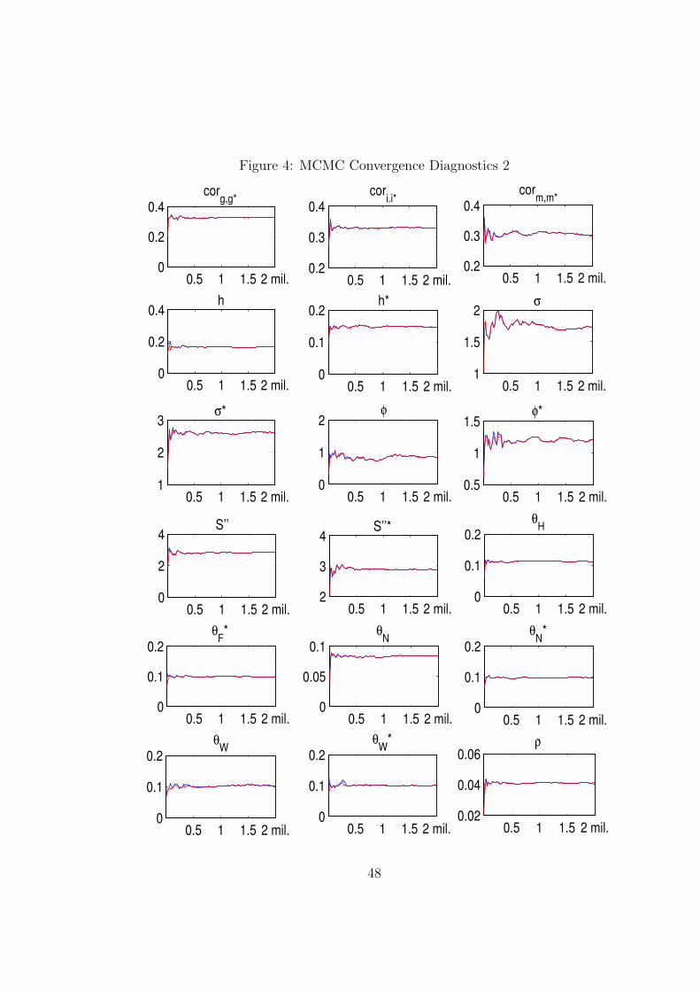
Figure 4: MCMC Convergence Diagnostics 2
0.5 1 1.5 2 mil.0
0.2
0.4cor
g,g*
0.5 1 1.5 2 mil.0.2
0.3
0.4cor
i.i*
0.5 1 1.5 2 mil.0.2
0.3
0.4cor
m,m*
0.5 1 1.5 2 mil.0
0.2
0.4h
0.5 1 1.5 2 mil.0
0.1
0.2h*
0.5 1 1.5 2 mil.1
1.5
2σ
0.5 1 1.5 2 mil.1
2
3σ*
0.5 1 1.5 2 mil.0
1
2φ
0.5 1 1.5 2 mil.0.5
1
1.5φ*
0.5 1 1.5 2 mil.0
2
4S’’
0.5 1 1.5 2 mil.2
3
4S’’*
0.5 1 1.5 2 mil.0
0.1
0.2θ
H
0.5 1 1.5 2 mil.0
0.1
0.2θ
F*
0.5 1 1.5 2 mil.0
0.05
0.1θ
N
0.5 1 1.5 2 mil.0
0.1
0.2θ
N*
0.5 1 1.5 2 mil.0
0.1
0.2θ
W
0.5 1 1.5 2 mil.0
0.1
0.2θ
W*
0.5 1 1.5 2 mil.0.02
0.04
0.06ρ
48

Figure 5: MCMC Convergence Diagnostics 3
0.5 1 1.5 2 mil.0.02
0.04
0.06ρ*
0.5 1 1.5 2 mil.0.04
0.06
0.08
ψy
0.5 1 1.5 2 mil.0.1
0.15
0.2ψ
y*
0.5 1 1.5 2 mil.0
0.2
0.4
ψπ
0.5 1 1.5 2 mil.0
0.5
1
ψπ*
0.5 1 1.5 2 mil.0
0.05
ρa
H
0.5 1 1.5 2 mil.0
0.2
0.4ρ
aF*
0.5 1 1.5 2 mil.0
0.2
0.4
ρa
N
0.5 1 1.5 2 mil.0
0.1
0.2ρ
aN*
0.5 1 1.5 2 mil.0
0.2
0.4ρ
d
0.5 1 1.5 2 mil.0
0.2
0.4
ρd*
0.5 1 1.5 2 mil.
0.2
0.25ρ
l
0.5 1 1.5 2 mil.0
0.2
0.4ρ
l*
0.5 1 1.5 2 mil.0
0.1
0.2ρ
g
0.5 1 1.5 2 mil.0
0.2
0.4ρ
g*
0.5 1 1.5 2 mil.0
0.1
0.2ρ
i
0.5 1 1.5 2 mil.0
0.1
0.2ρ
i*
49

References
[1] Brooks SP, Gelman A (1998): General Methods for Monitoring Conver-
gence of Iterative Simulations. Journal of Computational and Graphical
Statistics, 7(4):434-455.
50
Appendix - Smoothed Shocks
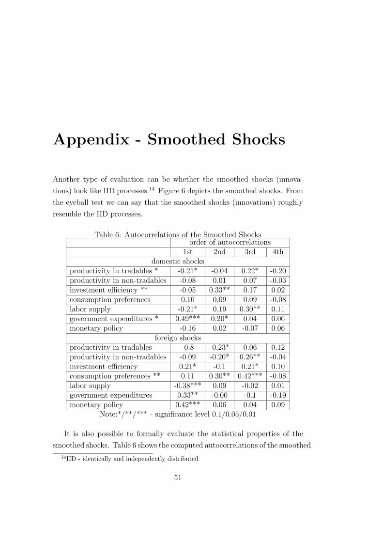
Another type of evaluation can be whether the smoothed shocks (innova-
tions) look like IID processes.14 Figure 6 depicts the smoothed shocks. From
the eyeball test we can say that the smoothed shocks (innovations) roughly
resemble the IID processes.
Table 6: Autocorrelations of the Smoothed Shocksorder of autocorrelations
1st 2nd 3rd 4thdomestic shocks
productivity in tradables * -0.21* -0.04 0.22* -0.20productivity in non-tradables -0.08 0.01 0.07 -0.03investment efficiency ** -0.05 0.33** 0.17 0.02consumption preferences 0.10 0.09 0.09 -0.08labor supply -0.21* 0.19 0.30** 0.11government expenditures * 0.49*** 0.20* 0.04 0.06monetary policy -0.16 0.02 -0.07 0.06
foreign shocksproductivity in tradables -0.8 -0.23* 0.06 0.12productivity in non-tradables -0.09 -0.20* 0.26** -0.04investment efficiency 0.21* -0.1 0.21* 0.10consumption preferences ** 0.11 0.30** 0.42*** -0.08labor supply -0.38*** 0.09 -0.02 0.01government expenditures 0.33** -0.00 -0.1 -0.19monetary policy 0.42*** 0.06 0.04 0.09
Note:*/**/*** - significance level 0.1/0.05/0.01
It is also possible to formally evaluate the statistical properties of the
smoothed shocks. Table 6 shows the computed autocorrelations of the smoothed
14IID - identically and independently distributed
51

shocks and their statistical significance (highlighted by the asterisks). Be-
sides testing statistical significance of each computed autocorrelation, it is
also possible to test the joint hypothesis that the shocks are independently
distributed, against the alternative hypothesis that the shocks are not in-
dependently distributed. This can be tested via the Ljung-Box Q test, see
Ljung and Box (1978). Let’s define the test statistic
Q = n(n+ 2)h∑k=1
ρ2kn− k
,
where n is the sample size, ρk is the sample autocorrelation at time lag k, and
h is the number of lags being tested (in this case h = 20). If the shocks are
independently distributed, then the test statistic Q is distributed according
to the chi-squared distribution with h degrees of freedom (i.e. Q ∼ χ2h). If
Q > χ21−α,h (χ2
1−α,h is the α-quantile of the chi-squared distribution with h
degrees of freedom), then we can reject the null hypothesis of randomness on
the significance level α. The results of this test are displayed in the Table
6, where rejections of the null hypothesis are highlighted by the asterisks in
the first column. The assumption of the independently distributed shocks
is violated only in the case of the domestic investment efficiency shock and
in the case of the foreign consumption preference shock (on the significance
level α = 0.05). We can see that the autocorrelation does not pose a serious
problem for most shocks.
52

Figure 6: Smoothed Shocks
2000 2002 2004 2006 2008 2010 2012−20
0
20
σa
H
2000 2002 2004 2006 2008 2010 2012−20
0
20
σa
F*
2000 2002 2004 2006 2008 2010 2012−50
0
50
σa
N
2000 2002 2004 2006 2008 2010 2012−10
0
10
σa
N*
2000 2002 2004 2006 2008 2010 2012−20
0
20
σd
2000 2002 2004 2006 2008 2010 2012−10
0
10
σd*
2000 2002 2004 2006 2008 2010 2012−200
0
200
σl
2000 2002 2004 2006 2008 2010 2012−100
0
100
σl*
2000 2002 2004 2006 2008 2010 2012−10
0
10
σg
2000 2002 2004 2006 2008 2010 2012−10
0
10
σg*
2000 2002 2004 2006 2008 2010 2012−20
0
20
σi
2000 2002 2004 2006 2008 2010 2012−20
0
20
σi*
2000 2002 2004 2006 2008 2010 2012−0.5
0
0.5
σm
2000 2002 2004 2006 2008 2010 2012−0.5
0
0.5
σm
*
53
References
[1] Ljung GM, Box GEP (1978): On a Measure of a Lack of Fit in Time
Series Models. Biometrika, 65(2):297-303.
54

Appendix - Predictions vs.
Observations
Quality of the model performance can be evaluated by comparison of the
k-step-ahead forecast of the observed variables with the actual realization
of the observed variables. Figure 7 displays one-step-ahead forecasts (green
line) and the observed values (blue line) for each observed variable. Figures
8 and 9 display 4-step-ahead forecasts (dashed lines) and observations (blue
solid line) of the most important observed variables: output, inflation and
interest rate.
From the eyeball test, we can see that the model is best in predicting
interest rates. The model also does a ”good job” in explaining the move-
ments in consumption, investment and GDP. On the other hand, real wage,
inflation, and internal exchange rate seem to have the worst fit among the
time series. It seems that the model does not fit these series quite well.
However, it is also possible to compare the model one-step-ahead pre-
dictions with the naıve predictions where the prediction is equal to the last
observed value. I can calculate the measure of fit of the predictions as the
Mean Square Error (MSE)
MSEM =
T∑t=2
(xmft − xobst )2
T − 1and MSEN =
T∑t=2
(xnft − xobst )2
T − 1,
where T is the number of observations, xmft is the model one-step-ahead
forecast for time t, xnft is the naıve one-step-ahead forecast for time t, xobst is
the observed value in time t, and MSEM (MSEN) stand for Mean Square
55

Error of the model (naıve) one-step-ahead forecasts. If I divide these two
measures I get
RFR =MSEMMSEN
,
where RFP stands for the ”relative forecast performance”. The measure
of relative forecast performance (RFP ) give us the formal evaluation of the
quality of the model forecast performance relatively to the performance of
the naıve forecasts. If the RFP is below one it indicates that the model
one-step-ahead forecast outperforms the naıve one-step-ahead forecast. On
the other hand, if the RFP is higher than one it indicates that the model
does a ”poor job” in explaining the movement of the particular observable
because the naıve one-step-ahead forecast outperforms the model one-step-
ahead forecast.
Table 7: Forecast Performance of the Observed Variablesobservable MSEM MSEN RFP
int. exchange rate CZ 0.6226 1.1783 0.5284int. exchange rate EA 12 0.3429 0.5850 0.5862real wage EA 12 0.4765 0.7656 0.6224interest rate CZ 0.0050 0.0079 0.6320interest rate EA 12 0.0088 0.0125 0.7053real wage CZ 1.8102 2.5514 0.7095GDP EA 12 0.3284 0.4576 0.7176HICP CZ 0.3786 0.4843 0.7816consumption EA 12 0.0560 0.0671 0.8342consumption CZ 0.2610 0.3033 0.8606investment EA 12 1.5673 1.7729 0.8840investment CZ 1.8860 2.0146 0.9362GDP CZ 0.9836 0.9664 1.0178HICP EA 12 0.1623 0.1568 1.0353
Table 7 displays calculated measures of the forecast performances. The
observed variables are ordered from the lowest RFP to the highest. We
can see that except for domestic output and foreign inflation, the model
one-step-ahead forecast outperforms the naıve one-step-ahead forecast. The
model is best in forecasting internal exchange rate, interest rate, real wage,
56

and foreign output. In case of domestic output and foreign inflation, the
naıve one-step-ahead forecast does a slightly better job than the model one-
step-ahead forecast, however, the difference is almost negligible.
A formal evaluation of the model forecast performance brings slightly
different results than which we can deduce from the eyeball test of Figure
7. It is so because the eyeball test does not take into account the different
volatility of the observables. If some observed variable is highly volatile,
then the naıve forecasts do not make much sense, and the model forecasts
are likely to do a much better job. On the other hand, if some variable is
not volatile too much, it is difficult for the model forecasts to outperform the
naıve forecasts.
57

Figure 7: Observed Variables and One-step-ahead Forecasts, green line -one-step-ahead forecast, blue line - observations
2000 2002 2004 2006 2008 2010 2012−2
0
2consumption CZ − demeaned 100*log differences
2000 2002 2004 2006 2008 2010 2012−1
0
1consumption EA12 − demeaned 100*log differences
2000 2002 2004 2006 2008 2010 2012−10
0
10investmet CZ − demeaned 100*log differences
2000 2002 2004 2006 2008 2010 2012−10
0
10investment EA12 − demeaned 100*log differences
2000 2002 2004 2006 2008 2010 2012−5
0
5GDP CZ − demeaned 100*log differences
2000 2002 2004 2006 2008 2010 2012−5
0
5GDP EA12 − demeaned 100*log differences
2000 2002 2004 2006 2008 2010 2012−5
0
5real wage CZ − demeaned 100*log differences
2000 2002 2004 2006 2008 2010 2012−5
0
5real wage EA12 − demeaned 100*log differences
2000 2002 2004 2006 2008 2010 2012−2
0
2HICP CZ − demeaned 100*log differences
2000 2002 2004 2006 2008 2010 2012−2
0
2HICP EA12 − demeaned 100*log differences
2000 2002 2004 2006 2008 2010 2012−5
0
5int. ex. rate CZ − demeaned 100*log differences
2000 2002 2004 2006 2008 2010 2012−5
0
5int. ex. rate EA12 − demeaned 100*log differences
2000 2002 2004 2006 2008 2010 2012−1
0
1interest rate CZ − demeaned quarterly rate
2000 2002 2004 2006 2008 2010 2012−1
0
1interest rate EA12 − demeaned quarterly rate
58

Figure 8: Observed Variables and 4-step-ahead Forecasts CZ, blue solid line- observations, dashed lines - 4-step-ahead forecasts
2000:2 2001:2 2002:2 2003:2 2004:2 2005:2 2006:2 2007:2 2008:2 2009:2 2010:2 2011:2
−4
−2
0
GDP CZ − demeaned 100*log differences
2000:2 2001:2 2002:2 2003:2 2004:2 2005:2 2006:2 2007:2 2008:2 2009:2 2010:2 2011:2
−1
0
1
HICP CZ − demeaned 100*log differences
2000:2 2001:2 2002:2 2003:2 2004:2 2005:2 2006:2 2007:2 2008:2 2009:2 2010:2 2011:2
−0.4
−0.2
0
0.2
0.4
0.6
interest rate CZ − demeaned quarterly rate
59

Figure 9: Observed Variables and 4-step-ahead Forecasts EA 12, blue solidline - observations, dashed lines - 4-step-ahead forecasts
2000:2 2001:2 2002:2 2003:2 2004:2 2005:2 2006:2 2007:2 2008:2 2009:2 2010:2 2011:2
−3
−2
−1
0
GDP EA 12 − demeaned 100*log differences
2000:2 2001:2 2002:2 2003:2 2004:2 2005:2 2006:2 2007:2 2008:2 2009:2 2010:2 2011:2
−1
−0.5
0
0.5
HICP EA 12 − demeaned 100*log differences
2000:2 2001:2 2002:2 2003:2 2004:2 2005:2 2006:2 2007:2 2008:2 2009:2 2010:2 2011:2
−0.5
0
0.5
interest rate EA 12 − demeaned quarterly rate
60

Appendix - Second Moments
I also evaluated the model performance by comparing selected second mo-
ments. I compared the second moments implied by the model with those im-
plied by the data and those implied by the unrestricted VAR(1) model, which
is treated as a benchmark. Figures 10-23 display calculated cross-correlations
among observed variables, Figure 24 displays variance of the observed vari-
ables, and Figures 25-27 display auto-correlations of the observed variables
up to the fourth order. Cross-correlations, variances, and auto-correlations
implied by the models are calculated analytically, see Hamilton (1994, p.
264-266). Every subfigure display values calculated for the model (red line),
for the data (green line), for the ”original” VAR(1) model (blue line), and for
the set of VAR(1) models (grey area) obtained from the ”original” VAR(1)
model by resampling residuals using wild bootstrap.15 Loosely speaking, this
set of resampled VAR(1) models serves as a confidence interval for the point
estimate obtained by the ”original” VAR(1) model. Ideally, we would like to
see that the model point estimate (red line) and the VAR(1) point estimate
(blue line) are close to the data estimate (green line).
We can see that the results for the data (green line) and for the VAR(1)
point estimate (blue line) are almost identical, which is not very surprising.
We can see that the model is able to replicate variance of most observed
variables, however, it fails in replicating variance of both domestic and foreign
inflation and variance of domestic interest rate and real wage. The model
implies much higher volatility of these variables than it is in the data. There
15Each residual is randomly multiplied by a random variable with mean 0 and variance1. This method assumes that the ’true’ residual distribution is symmetric and can offeradvantages over simple residual sampling for smaller sample sizes. See Wu (1986) and Liu(1988).
61

are also significant differences in autocorrelations of output and inflation.
The model implies much lower autocorrelation of both domestic and foreign
output than which can be found in the data, while for inflation the model
implies much higher autocorrelation than which can be found in the data.
The results for cross-correlations are, not surprisingly, quite unsuccessful.
The model implies much lower cross-correlations for most variables than the
data. However, this is a well-known weakness of New Keynesian DSGE
models.
Figure 10: Cross-Correlations of Domestic Output
−1 −0.5 0 0.5 10
100
200
Yobs
with Yobs*
−1 −0.5 0 0.5 10
100
200
Yobs
with Cobs
−1 −0.5 0 0.5 10
100
200
Yobs
with Cobs*
−1 −0.5 0 0.5 10
100
200
Yobs
with Iobs
−1 −0.5 0 0.5 10
200
Yobs
with Iobs*
−1 −0.5 0 0.5 10
100
Yobs
with HICPobs
−1 −0.5 0 0.5 10
100
Yobs
with HICPobs*
−1 −0.5 0 0.5 10
100
200
Yobs
with Robs
−1 −0.5 0 0.5 10
100
200
Yobs
with Robs*
−1 −0.5 0 0.5 10
200
Yobs
with Wobs
−1 −0.5 0 0.5 10
100
200
Yobs
with Wobs*
−1 −0.5 0 0.5 10
100
200
Yobs
with Xobs
−1 −0.5 0 0.5 10
200
Yobs
with Xobs*
VAR: bootstrap
VAR: point estimate
Model
Data
62

Figure 11: Cross-Correlations of Foreign Output
−1 −0.5 0 0.5 10
100
200
Yobs*
with Yobs
−1 −0.5 0 0.5 10
100
200
Yobs*
with Cobs
−1 −0.5 0 0.5 10
100
200
Yobs*
with Cobs*
−1 −0.5 0 0.5 10
100
200
Yobs*
with Iobs
−1 −0.5 0 0.5 10
100
200
Yobs*
with Iobs*
−1 −0.5 0 0.5 10
100
200
Yobs*
with HICPobs
−1 −0.5 0 0.5 10
100
200
Yobs*
with HICPobs*
−1 −0.5 0 0.5 10
100
200
Yobs*
with Robs
−1 −0.5 0 0.5 10
200
Yobs*
with Robs*
−1 −0.5 0 0.5 10
100
200
Yobs*
with Wobs
−1 −0.5 0 0.5 10
100
200
Yobs*
with Wobs*
−1 −0.5 0 0.5 10
100
200
Yobs*
with Xobs
−1 −0.5 0 0.5 10
100
200
Yobs*
with Xobs*
VAR: bootstrap
VAR: point estimate
Model
Data
Figure 12: Cross-Correlations of Domestic Consumption
−1 −0.5 0 0.5 10
100
200
Cobs
with Yobs
−1 −0.5 0 0.5 10
100
200
Cobs
with Yobs*
−1 −0.5 0 0.5 10
100
200
Cobs
with Cobs*
−1 −0.5 0 0.5 10
100
200
Cobs
with Iobs
−1 −0.5 0 0.5 10
100
200
Cobs
with Iobs*
−1 −0.5 0 0.5 10
100
200
Cobs
with HICPobs
−1 −0.5 0 0.5 10
100
200
Cobs
with HICPobs*
−1 −0.5 0 0.5 10
100
200
Cobs
with Robs
−1 −0.5 0 0.5 10
100
200
Cobs
with Robs*
−1 −0.5 0 0.5 10
100
200
Cobs
with Wobs
−1 −0.5 0 0.5 10
100
200
Cobs
with Wobs*
−1 −0.5 0 0.5 10
100
200
Cobs
with Xobs
−1 −0.5 0 0.5 10
100
200
Cobs
with Xobs*
VAR: bootstrap
VAR: point estimate
Model
Data
63

Figure 13: Cross-Correlations of Foreign Consumption
−1 −0.5 0 0.5 10
100
200
Cobs*
with Yobs
−1 −0.5 0 0.5 10
100
200
Cobs*
with Yobs*
−1 −0.5 0 0.5 10
100
200
Cobs*
with Cobs
−1 −0.5 0 0.5 10
100
200
Cobs*
with Iobs
−1 −0.5 0 0.5 10
100
Cobs*
with Iobs*
−1 −0.5 0 0.5 10
100
200
Cobs*
with HICPobs
−1 −0.5 0 0.5 10
100
200
Cobs*
with HICPobs*
−1 −0.5 0 0.5 10
100
200
Cobs*
with Robs
−1 −0.5 0 0.5 10
100
200
Cobs*
with Robs*
−1 −0.5 0 0.5 10
100
200
Cobs*
with Wobs
−1 −0.5 0 0.5 10
100
200
Cobs*
with Wobs*
−1 −0.5 0 0.5 10
100
200
Cobs*
with Xobs
−1 −0.5 0 0.5 10
100
200
Cobs*
with Xobs*
VAR: bootstrap
VAR: point estimate
Model
Data
Figure 14: Cross-Correlations of Domestic Investment
−1 −0.5 0 0.5 10
100
200
Iobs
with Yobs
−1 −0.5 0 0.5 10
100
200
Iobs
with Yobs*
−1 −0.5 0 0.5 10
100
200
Iobs
with Cobs
−1 −0.5 0 0.5 10
100
200
Iobs
with Cobs*
−1 −0.5 0 0.5 10
100
200
Iobs
with Iobs*
−1 −0.5 0 0.5 10
100
200
Iobs
with HICPobs
−1 −0.5 0 0.5 10
100
200
Iobs
with HICPobs*
−1 −0.5 0 0.5 10
100
200
Iobs
with Robs
−1 −0.5 0 0.5 10
100
200
Iobs
with Robs*
−1 −0.5 0 0.5 10
200
Iobs
with Wobs
−1 −0.5 0 0.5 10
100
200
Iobs
with Wobs*
−1 −0.5 0 0.5 10
100
200
Iobs
with Xobs
−1 −0.5 0 0.5 10
100
200
Iobs
with Xobs*
VAR: bootstrap
VAR: point estimate
Model
Data
64
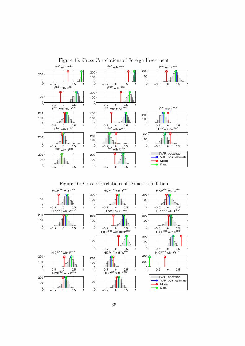
Figure 15: Cross-Correlations of Foreign Investment
−1 −0.5 0 0.5 10
200
Iobs*
with Yobs
−1 −0.5 0 0.5 10
100
200
Iobs*
with Yobs*
−1 −0.5 0 0.5 10
100
200
Iobs*
with Cobs
−1 −0.5 0 0.5 10
100
Iobs*
with Cobs*
−1 −0.5 0 0.5 10
100
200
Iobs*
with Iobs
−1 −0.5 0 0.5 10
100
200
Iobs*
with HICPobs
−1 −0.5 0 0.5 10
100
200
Iobs*
with HICPobs*
−1 −0.5 0 0.5 10
100
200
Iobs*
with Robs
−1 −0.5 0 0.5 10
200
Iobs*
with Robs*
−1 −0.5 0 0.5 10
100
200
Iobs*
with Wobs
−1 −0.5 0 0.5 10
100
200
Iobs*
with Wobs*
−1 −0.5 0 0.5 10
100
200
Iobs*
with Xobs
−1 −0.5 0 0.5 10
100
200
Iobs*
with Xobs*
VAR: bootstrap
VAR: point estimate
Model
Data
Figure 16: Cross-Correlations of Domestic Inflation
−1 −0.5 0 0.5 10
100
HICPobs
with Yobs
−1 −0.5 0 0.5 10
100
200
HICPobs
with Yobs*
−1 −0.5 0 0.5 10
100
200
HICPobs
with Cobs
−1 −0.5 0 0.5 10
100
200
HICPobs
with Cobs*
−1 −0.5 0 0.5 10
100
200
HICPobs
with Iobs
−1 −0.5 0 0.5 10
100
200
HICPobs
with Iobs*
−1 −0.5 0 0.5 10
100
HICPobs
with HICPobs*
−1 −0.5 0 0.5 10
100
200
HICPobs
with Robs
−1 −0.5 0 0.5 10
100
200
HICPobs
with Robs*
−1 −0.5 0 0.5 10
100
200
HICPobs
with Wobs
−1 −0.5 0 0.5 10
200
400
HICPobs
with Wobs*
−1 −0.5 0 0.5 10
100
200
HICPobs
with Xobs
−1 −0.5 0 0.5 10
100
HICPobs
with Xobs*
VAR: bootstrap
VAR: point estimate
Model
Data
65

Figure 17: Cross-Correlations of Foreign Inflation
−1 −0.5 0 0.5 10
100
HICPobs*
with Yobs
−1 −0.5 0 0.5 10
100
200
HICPobs*
with Yobs*
−1 −0.5 0 0.5 10
100
200
HICPobs*
with Cobs
−1 −0.5 0 0.5 10
100
200
HICPobs*
with Cobs*
−1 −0.5 0 0.5 10
100
200
HICPobs*
with Iobs
−1 −0.5 0 0.5 10
100
200
HICPobs*
with Iobs*
−1 −0.5 0 0.5 10
100
HICPobs*
with HICPobs
−1 −0.5 0 0.5 10
200
HICPobs*
with Robs
−1 −0.5 0 0.5 10
200
HICPobs*
with Robs*
−1 −0.5 0 0.5 10
100
200
HICPobs*
with Wobs
−1 −0.5 0 0.5 10
100
200
HICPobs*
with Wobs*
−1 −0.5 0 0.5 10
100
200
HICPobs*
with Xobs
−1 −0.5 0 0.5 10
200
HICPobs*
with Xobs*
VAR: bootstrap
VAR: point estimate
Model
Data
Figure 18: Cross-Correlations of Domestic Interest Rate
−1 −0.5 0 0.5 10
100
200
Robs
with Yobs
−1 −0.5 0 0.5 10
100
200
Robs
with Yobs*
−1 −0.5 0 0.5 10
100
200
Robs
with Cobs
−1 −0.5 0 0.5 10
100
200
Robs
with Cobs*
−1 −0.5 0 0.5 10
100
200
Robs
with Iobs
−1 −0.5 0 0.5 10
100
200
Robs
with Iobs*
−1 −0.5 0 0.5 10
100
200
Robs
with HICPobs
−1 −0.5 0 0.5 10
200
Robs
with HICPobs*
−1 −0.5 0 0.5 10
100
200
Robs
with Robs*
−1 −0.5 0 0.5 10
100
200
Robs
with Wobs
−1 −0.5 0 0.5 10
100
200
Robs
with Wobs*
−1 −0.5 0 0.5 10
100
200
Robs
with Xobs
−1 −0.5 0 0.5 10
100
200
Robs
with Xobs*
VAR: bootstrap
VAR: point estimate
Model
Data
66

Figure 19: Cross-Correlations of Foreign Interest Rate
−1 −0.5 0 0.5 10
100
200
Robs*
with Yobs
−1 −0.5 0 0.5 10
200
Robs*
with Yobs*
−1 −0.5 0 0.5 10
100
200
Robs*
with Cobs
−1 −0.5 0 0.5 10
100
200
Robs*
with Cobs*
−1 −0.5 0 0.5 10
100
200
Robs*
with Iobs
−1 −0.5 0 0.5 10
200
Robs*
with Iobs*
−1 −0.5 0 0.5 10
100
200
Robs*
with HICPobs
−1 −0.5 0 0.5 10
200
Robs*
with HICPobs*
−1 −0.5 0 0.5 10
100
200
Robs*
with Robs
−1 −0.5 0 0.5 10
100
200
Robs*
with Wobs
−1 −0.5 0 0.5 10
100
Robs*
with Wobs*
−1 −0.5 0 0.5 10
100
200
Robs*
with Xobs
−1 −0.5 0 0.5 10
100
200
Robs*
with Xobs*
VAR: bootstrap
VAR: point estimate
Model
Data
Figure 20: Cross-Correlations of Domestic Real Wage
−1 −0.5 0 0.5 10
200
Wobs
with Yobs
−1 −0.5 0 0.5 10
100
200
Wobs
with Yobs*
−1 −0.5 0 0.5 10
100
200
Wobs
with Cobs
−1 −0.5 0 0.5 10
100
200
Wobs
with Cobs*
−1 −0.5 0 0.5 10
200
Wobs
with Iobs
−1 −0.5 0 0.5 10
100
200
Wobs
with Iobs*
−1 −0.5 0 0.5 10
100
200
Wobs
with HICPobs
−1 −0.5 0 0.5 10
100
200
Wobs
with HICPobs*
−1 −0.5 0 0.5 10
100
200
Wobs
with Robs
−1 −0.5 0 0.5 10
100
200
Wobs
with Robs*
−1 −0.5 0 0.5 10
100
Wobs
with Wobs*
−1 −0.5 0 0.5 10
100
Wobs
with Xobs
−1 −0.5 0 0.5 10
100
200
Wobs
with Xobs*
VAR: bootstrap
VAR: point estimate
Model
Data
67

Figure 21: Cross-Correlations of Foreign Real Wage
−1 −0.5 0 0.5 10
100
200
Wobs*
with Yobs
−1 −0.5 0 0.5 10
100
200
Wobs*
with Yobs*
−1 −0.5 0 0.5 10
100
200
Wobs*
with Cobs
−1 −0.5 0 0.5 10
100
200
Wobs*
with Cobs*
−1 −0.5 0 0.5 10
100
200
Wobs*
with Iobs
−1 −0.5 0 0.5 10
100
200
Wobs*
with Iobs*
−1 −0.5 0 0.5 10
200
400
Wobs*
with HICPobs
−1 −0.5 0 0.5 10
100
200
Wobs*
with HICPobs*
−1 −0.5 0 0.5 10
100
200
Wobs*
with Robs
−1 −0.5 0 0.5 10
100
Wobs*
with Robs*
−1 −0.5 0 0.5 10
100
Wobs*
with Wobs
−1 −0.5 0 0.5 10
100
200
Wobs*
with Xobs
−1 −0.5 0 0.5 10
100
Wobs*
with Xobs*
VAR: bootstrap
VAR: point estimate
Model
Data
Figure 22: Cross-Correlations of Domestic Internal Exchange Rate
−1 −0.5 0 0.5 10
100
200
Xobs
with Yobs
−1 −0.5 0 0.5 10
100
200
Xobs
with Yobs*
−1 −0.5 0 0.5 10
100
200
Xobs
with Cobs
−1 −0.5 0 0.5 10
100
200
Xobs
with Cobs*
−1 −0.5 0 0.5 10
100
200
Xobs
with Iobs
−1 −0.5 0 0.5 10
100
200
Xobs
with Iobs*
−1 −0.5 0 0.5 10
100
200
Xobs
with HICPobs
−1 −0.5 0 0.5 10
100
200
Xobs
with HICPobs*
−1 −0.5 0 0.5 10
100
200
Xobs
with Robs
−1 −0.5 0 0.5 10
100
200
Xobs
with Robs*
−1 −0.5 0 0.5 10
100
Xobs
with Wobs
−1 −0.5 0 0.5 10
100
200
Xobs
with Wobs*
−1 −0.5 0 0.5 10
100
Xobs
with Xobs*
VAR: bootstrap
VAR: point estimate
Model
Data
68

Figure 23: Cross-Correlations of Foreign Internal Exchange Rate
−1 −0.5 0 0.5 10
200
Xobs*
with Yobs
−1 −0.5 0 0.5 10
100
200
Xobs*
with Yobs*
−1 −0.5 0 0.5 10
100
200
Xobs*
with Cobs
−1 −0.5 0 0.5 10
100
200
Xobs*
with Cobs*
−1 −0.5 0 0.5 10
100
200
Xobs*
with Iobs
−1 −0.5 0 0.5 10
100
200
Xobs*
with Iobs*
−1 −0.5 0 0.5 10
100
Xobs*
with HICPobs
−1 −0.5 0 0.5 10
200
Xobs*
with HICPobs*
−1 −0.5 0 0.5 10
100
200
Xobs*
with Robs
−1 −0.5 0 0.5 10
100
200
Xobs*
with Robs*
−1 −0.5 0 0.5 10
100
200
Xobs*
with Wobs
−1 −0.5 0 0.5 10
100
Xobs*
with Wobs*
−1 −0.5 0 0.5 10
100
Xobs*
with Xobs
VAR: bootstrap
VAR: point estimate
Model
Data
Figure 24: Variance of Observables
0 5 10 15 200
1000
2000Variance of Y
obs
0 5 100
500
1000Variance of Y
obs*
0 1 2 30
500
1000Variance of C
obs
0 0.5 1 1.50
500
1000Variance of C
obs*
0 20 40 60 800
1000
2000Variance of I
obs
0 20 40 600
1000
2000Variance of I
obs*
0 1 2 3 40
500
1000Variance of HICP
obs
0 0.5 1 1.50
500
1000Variance of HICP
obs*
0 0.5 1 1.50
500
1000Variance of R
obs
0 1 2 30
1000
2000Variance of R
obs*
0 1 2 3 40
200
400Variance of W
obs
0 1 2 30
500
1000Variance of W
obs*
0 0.5 1 1.5 20
200
400Variance of X
obs
0 1 2 30
500
1000Variance of X
obs*
VAR: bootstrap
VAR: point estimate
Model
Data
69

Figure 25: Auto-Correlation Functions 1
−1 0 10
100
200
Yobs
− ACF(1)
−1 0 10
100
200Y
obs− ACF(2)
−1 0 10
100
200
Yobs
− ACF(3)
−1 0 10
100
200
Yobs
− ACF(4)
−1 0 10
100
200
Yobs*
− ACF(1)
−1 0 10
100
200
Yobs*
− ACF(2)
−1 0 10
100
Yobs*
− ACF(3)
−1 0 10
100
200
Yobs*
− ACF(4)
−1 0 10
100
Cobs
− ACF(1)
−1 0 10
100
Cobs
− ACF(2)
−1 0 10
100
Cobs
− ACF(3)
−1 0 10
100
200
Cobs
− ACF(4)
−1 0 10
100
Cobs*
− ACF(1)
−1 0 10
100
Cobs*
− ACF(2)
−1 0 10
100
200
Cobs*
− ACF(3)
−1 0 10
100
200
Cobs*
− ACF(4)
−1 0 10
100
200
Iobs
− ACF(1)
−1 0 10
100
Iobs
− ACF(2)
−1 0 10
100
Iobs
− ACF(3)
−1 0 10
100
200
Iobs
− ACF(4)
Figure 26: Auto-Correlation Functions 2
−1 0 10
100
Iobs*
− ACF(1)
−1 0 10
100
Iobs*
− ACF(2)
−1 0 10
100
Iobs*
− ACF(3)
−1 0 10
100
200
Iobs*
− ACF(4)
−1 0 10
100
200
HICPobs
− ACF(1)
−1 0 10
100
200
HICPobs
− ACF(2)
−1 0 10
200
HICPobs
− ACF(3)
−1 0 10
200
HICPobs
− ACF(4)
−1 0 10
100
HICPobs*
− ACF(1)
−1 0 10
100
200
HICPobs*
− ACF(2)
−1 0 10
100
200
HICPobs*
− ACF(3)
−1 0 10
100
200
HICPobs*
− ACF(4)
−1 0 10
200
Robs
− ACF(1)
−1 0 10
100
200
Robs
− ACF(2)
−1 0 10
100
200
Robs
− ACF(3)
−1 0 10
100
200
Robs
− ACF(4)
−1 0 10
100
200
Robs*
− ACF(1)
−1 0 10
100
200
Robs*
− ACF(2)
−1 0 10
100
200
Robs*
− ACF(3)
−1 0 10
100
200
Robs*
− ACF(4)
70

Figure 27: Auto-Correlation Functions 3
−1 0 10
100
200
Wobs
− ACF(1)
−1 0 10
100
200
Wobs
− ACF(2)
−1 0 10
100
200
Wobs
− ACF(3)
−1 0 10
100
200
Wobs
− ACF(4)
−1 0 10
100
200
Wobs*
− ACF(1)
−1 0 10
100
200
Wobs*
− ACF(2)
−1 0 10
100
200
Wobs*
− ACF(3)
−1 0 10
100
200
Wobs*
− ACF(4)
−1 0 10
100
200
Xobs
− ACF(1)
−1 0 10
100
200
Xobs
− ACF(2)
−1 0 10
100
200
Xobs
− ACF(3)
−1 0 10
100
200
Xobs
− ACF(4)
−1 0 10
100
200
Xobs*
− ACF(1)
−1 0 10
100
200
Xobs*
− ACF(2)
−1 0 10
100
Xobs*
− ACF(3)
−1 0 10
100
200
Xobs*
− ACF(4)
VAR: bootstrap
VAR: point estimate
Model
Data
71
References
[1] Hamilton JJ (1994): Time Series Analysis. Princeton University Press,
Princeton.
[2] Liu RY (1988): Bootstrap Procedures under some Non-I.I.D. Models.
Annals of Statistics, 16(4):1696-1708.
[3] Wu CFJ (1986): Jackknife, Bootstrap and Other Resampling Methods
in Regression Analysis. Annals of Statistics, 14(4):1261-1350.
72

Spectral Analysis
Figure 28 displays spectrum density functions of the observed variables for
the model and for the VAR(1) model. The vertical lines highlight the fre-
quencies which correspond to periods of 1 quarter and 10 quarters.
Figure 28: Spectrum Density Functions
0 2−1
0
1Y
obs
0 2−1
0
1Y
obs*
0 2−1
0
1C
obs
0 2−1
0
1C
obs*
0 20
1
2Iobs
0 20
0.5
1Iobs*
0 20
2
4HICP
obs
0 20
2
4HICP
obs*
0 20
5
10R
obs
0 20
5
10R
obs*
0 2−0.5
0
0.5W
obs
0 20
0.2
0.4W
obs*
0 2−0.5
0
0.5X
obs
0 2−0.5
0
0.5X
obs*
VAR: point estimate
Model
73

Appendix - Shock
Decomposition
Shock decomposition displays individual contributions of the shocks to the
deviations of the examined variable from its respective steady state. Evolu-
tion of the examined variable is in every period decomposed into the contri-
butions of the structural shocks.
Figure 29: Shock Decomposition of Observables - Domestic Output
2000 2002 2004 2006 2008 2010 2012
−600
−500
−400
−300
−200
−100
0
100
200
time
domestic monetary policy shock
foreign monetary policy shock
domestic shock in government expenditures
foreign shock in government expenditures
domestic consumption preference shock
foreign consumption preference shock
domestic investment efficiency shock
foreign investment efficiency shock
domestic productivityshock in tradables
foreign productivity shock in tradables
domestic productivityshock in non−tradables
foreign productivity shock in non−tradables
domestic labor supply shock
foreign labor supply shock
initial values
74

Figure 30: Shock Decomposition of Observables - Foreign Output
2000 2002 2004 2006 2008 2010 2012
−350
−300
−250
−200
−150
−100
−50
0
50
100
time
domestic monetary policy shock
foreign monetary policy shock
domestic shock in government expenditures
foreign shock in government expenditures
domestic consumption preference shock
foreign consumption preference shock
domestic investment efficiency shock
foreign investment efficiency shock
domestic productivityshock in tradables
foreign productivity shock in tradables
domestic productivityshock in non−tradables
foreign productivity shock in non−tradables
domestic labor supply shock
foreign labor supply shock
initial values
Figure 31: Shock Decomposition of Observables - Domestic Consumption
2000 2002 2004 2006 2008 2010 2012−200
−150
−100
−50
0
50
100
150
time
domestic monetary policy shock
foreign monetary policy shock
domestic shock in government expenditures
foreign shock in government expenditures
domestic consumption preference shock
foreign consumption preference shock
domestic investment efficiency shock
foreign investment efficiency shock
domestic productivityshock in tradables
foreign productivity shock in tradables
domestic productivityshock in non−tradables
foreign productivity shock in non−tradables
domestic labor supply shock
foreign labor supply shock
initial values
75

Figure 32: Shock Decomposition of Observables - Foreign Consumption
2000 2002 2004 2006 2008 2010 2012
−100
−80
−60
−40
−20
0
20
40
60
time
domestic monetary policy shock
foreign monetary policy shock
domestic shock in government expenditures
foreign shock in government expenditures
domestic consumption preference shock
foreign consumption preference shock
domestic investment efficiency shock
foreign investment efficiency shock
domestic productivityshock in tradables
foreign productivity shock in tradables
domestic productivityshock in non−tradables
foreign productivity shock in non−tradables
domestic labor supply shock
foreign labor supply shock
initial values
Figure 33: Shock Decomposition of Observables - Domestic Investment
2000 2002 2004 2006 2008 2010 2012
−600
−400
−200
0
200
400
time
domestic monetary policy shock
foreign monetary policy shock
domestic shock in government expenditures
foreign shock in government expenditures
domestic consumption preference shock
foreign consumption preference shock
domestic investment efficiency shock
foreign investment efficiency shock
domestic productivityshock in tradables
foreign productivity shock in tradables
domestic productivityshock in non−tradables
foreign productivity shock in non−tradables
domestic labor supply shock
foreign labor supply shock
initial values
76

Figure 34: Shock Decomposition of Observables - Foreign Investment
2000 2002 2004 2006 2008 2010 2012−1000
−800
−600
−400
−200
0
200
time
domestic monetary policy shock
foreign monetary policy shock
domestic shock in government expenditures
foreign shock in government expenditures
domestic consumption preference shock
foreign consumption preference shock
domestic investment efficiency shock
foreign investment efficiency shock
domestic productivityshock in tradables
foreign productivity shock in tradables
domestic productivityshock in non−tradables
foreign productivity shock in non−tradables
domestic labor supply shock
foreign labor supply shock
initial values
Figure 35: Shock Decomposition of Observables - Domestic Interest Rate
2000 2002 2004 2006 2008 2010 2012
−100
−80
−60
−40
−20
0
20
40
60
80
100
time
domestic monetary policy shock
foreign monetary policy shock
domestic shock in government expenditures
foreign shock in government expenditures
domestic consumption preference shock
foreign consumption preference shock
domestic investment efficiency shock
foreign investment efficiency shock
domestic productivityshock in tradables
foreign productivity shock in tradables
domestic productivityshock in non−tradables
foreign productivity shock in non−tradables
domestic labor supply shock
foreign labor supply shock
initial values
77

Figure 36: Shock Decomposition of Observables - Foreign Interest Rate
2000 2002 2004 2006 2008 2010 2012
−60
−40
−20
0
20
40
60
time
domestic monetary policy shock
foreign monetary policy shock
domestic shock in government expenditures
foreign shock in government expenditures
domestic consumption preference shock
foreign consumption preference shock
domestic investment efficiency shock
foreign investment efficiency shock
domestic productivityshock in tradables
foreign productivity shock in tradables
domestic productivityshock in non−tradables
foreign productivity shock in non−tradables
domestic labor supply shock
foreign labor supply shock
initial values
Figure 37: Shock Decomposition of Observables - Domestic Inflation
2000 2002 2004 2006 2008 2010 2012−400
−300
−200
−100
0
100
200
300
400
500
time
domestic monetary policy shock
foreign monetary policy shock
domestic shock in government expenditures
foreign shock in government expenditures
domestic consumption preference shock
foreign consumption preference shock
domestic investment efficiency shock
foreign investment efficiency shock
domestic productivityshock in tradables
foreign productivity shock in tradables
domestic productivityshock in non−tradables
foreign productivity shock in non−tradables
domestic labor supply shock
foreign labor supply shock
initial values
78

Figure 38: Shock Decomposition of Observables - Foreign Inflation
2000 2002 2004 2006 2008 2010 2012
−300
−250
−200
−150
−100
−50
0
50
100
150
200
time
domestic monetary policy shock
foreign monetary policy shock
domestic shock in government expenditures
foreign shock in government expenditures
domestic consumption preference shock
foreign consumption preference shock
domestic investment efficiency shock
foreign investment efficiency shock
domestic productivityshock in tradables
foreign productivity shock in tradables
domestic productivityshock in non−tradables
foreign productivity shock in non−tradables
domestic labor supply shock
foreign labor supply shock
initial values
Figure 39: Shock Decomposition of Observables - Domestic Real Wage
2000 2002 2004 2006 2008 2010 2012
−500
−400
−300
−200
−100
0
100
200
300
400
500
time
domestic monetary policy shock
foreign monetary policy shock
domestic shock in government expenditures
foreign shock in government expenditures
domestic consumption preference shock
foreign consumption preference shock
domestic investment efficiency shock
foreign investment efficiency shock
domestic productivityshock in tradables
foreign productivity shock in tradables
domestic productivityshock in non−tradables
foreign productivity shock in non−tradables
domestic labor supply shock
foreign labor supply shock
initial values
79
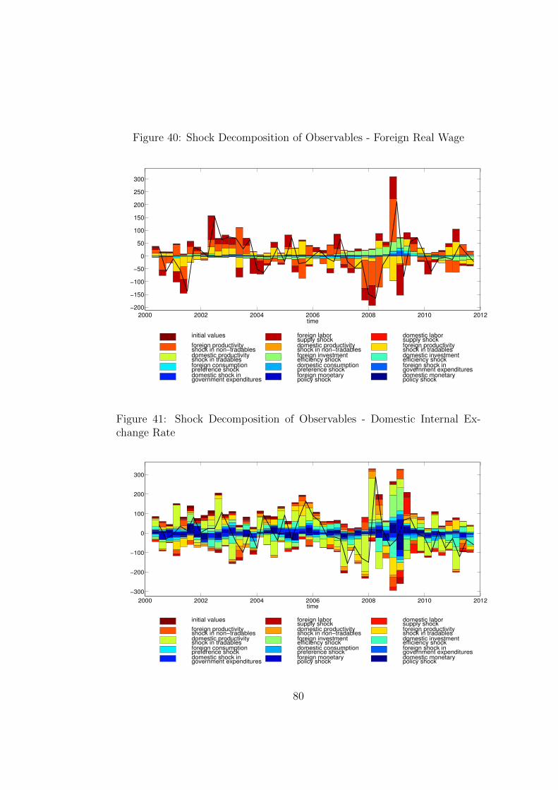
Figure 40: Shock Decomposition of Observables - Foreign Real Wage
2000 2002 2004 2006 2008 2010 2012
−200
−150
−100
−50
0
50
100
150
200
250
300
time
domestic monetary policy shock
foreign monetary policy shock
domestic shock in government expenditures
foreign shock in government expenditures
domestic consumption preference shock
foreign consumption preference shock
domestic investment efficiency shock
foreign investment efficiency shock
domestic productivityshock in tradables
foreign productivity shock in tradables
domestic productivityshock in non−tradables
foreign productivity shock in non−tradables
domestic labor supply shock
foreign labor supply shock
initial values
Figure 41: Shock Decomposition of Observables - Domestic Internal Ex-change Rate
2000 2002 2004 2006 2008 2010 2012
−300
−200
−100
0
100
200
300
time
domestic monetary policy shock
foreign monetary policy shock
domestic shock in government expenditures
foreign shock in government expenditures
domestic consumption preference shock
foreign consumption preference shock
domestic investment efficiency shock
foreign investment efficiency shock
domestic productivityshock in tradables
foreign productivity shock in tradables
domestic productivityshock in non−tradables
foreign productivity shock in non−tradables
domestic labor supply shock
foreign labor supply shock
initial values
80

Figure 42: Shock Decomposition of Observables - Foreign Internal ExchangeRate
2000 2002 2004 2006 2008 2010 2012−250
−200
−150
−100
−50
0
50
100
time
domestic monetary policy shock
foreign monetary policy shock
domestic shock in government expenditures
foreign shock in government expenditures
domestic consumption preference shock
foreign consumption preference shock
domestic investment efficiency shock
foreign investment efficiency shock
domestic productivityshock in tradables
foreign productivity shock in tradables
domestic productivityshock in non−tradables
foreign productivity shock in non−tradables
domestic labor supply shock
foreign labor supply shock
initial values
81
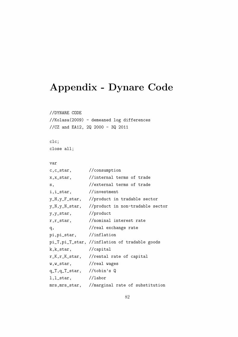
Appendix - Dynare Code
//DYNARE CODE
//Kolasa(2009) - demeaned log differences
//CZ and EA12, 2Q 2000 - 3Q 2011
clc;
close all;
var
c,c_star, //consumption
x,x_star, //internal terms of trade
s, //external terms of trade
i,i_star, //investment
y_H,y_F_star, //product in tradable sector
y_N,y_N_star, //product in non-tradable sector
y,y_star, //product
r,r_star, //nominal interest rate
q, //real exchange rate
pi,pi_star, //inflation
pi_T,pi_T_star, //inflation of tradable goods
k,k_star, //capital
r_K,r_K_star, //rental rate of capital
w,w_star, //real wages
q_T,q_T_star, //tobin’s Q
l,l_star, //labor
mrs,mrs_star, //marginal rate of substitution
82

pi_H,pi_F_star, //inflation of raw tradable goods
mc_H,mc_F_star, //real marginal costs in tradable sector
pi_N,pi_N_star, //inflation of non-tradable goods
mc_N,mc_N_star, //real marginal costs in non-tradable sector
//Observables
y_obs, y_star_obs,
c_obs, c_star_obs,
i_obs, i_star_obs,
r_obs, r_star_obs,
pi_obs, pi_star_obs,
w_obs, w_star_obs,
x_obs, x_star_obs,
//AR processes for shocks
epsilon_g,epsilon_g_star,
epsilon_d,epsilon_d_star,
epsilon_i,epsilon_i_star,
epsilon_a_H,epsilon_a_F_star,
epsilon_a_N,epsilon_a_N_star,
epsilon_l,epsilon_l_star;
varexo
epsilon_m,epsilon_m_star,
mu_g,mu_g_star,
mu_d,mu_d_star,
mu_i,mu_i_star,
mu_a_H,mu_a_F_star,
mu_a_N,mu_a_N_star,
mu_l,mu_l_star;
parameters
beta, beta_star, //discount factor
83

gamma_c,gamma_c_star, //share of tradable goods in consumption
gamma_i,gamma_i_star, //share of tradable goods in investment
alpha,alpha_star, //share of domestic tradable goods
omega,omega_star, //share of distribution costs
n, //relative size of economies
h,h_star, //habit formation
sigma,sigma_star, //inv. elasticity of intertemporal subs.
tau,tau_star, //depreciation rate
S_prime,S_prime_star, //adjustment costs
eta,eta_star, //elasticity of output wrt capital
theta_W,theta_W_star, //Calvo parameters for households
delta_W,delta_W_star, //wage indexation
phi_W,phi_W_star, //elasticity of subst. among labor types
phi,phi_star, //inv. elasticity of labor supply
delta_H,delta_F_star, //indexation of tradables
theta_H,theta_F_star, //Calvo parameters for tradables
delta_N,delta_N_star, //indexation of non-tradables
theta_N,theta_N_star, //Calvo parameters for non-tradables
rho,rho_star, //interest rate smoothing
psi_y,psi_y_star, //elasticity of interest rate to output
psi_pi,psi_pi_star, //elast. of interest rate to inflation
//persistence of shocks
rho_a_H, rho_a_F_star,
rho_a_N, rho_a_N_star,
rho_d, rho_d_star,
rho_l, rho_l_star,
rho_g, rho_g_star,
rho_i, rho_i_star,
//shares of variables in steady-state
ss_C_Y,
ss_C_star_Y_star,
84
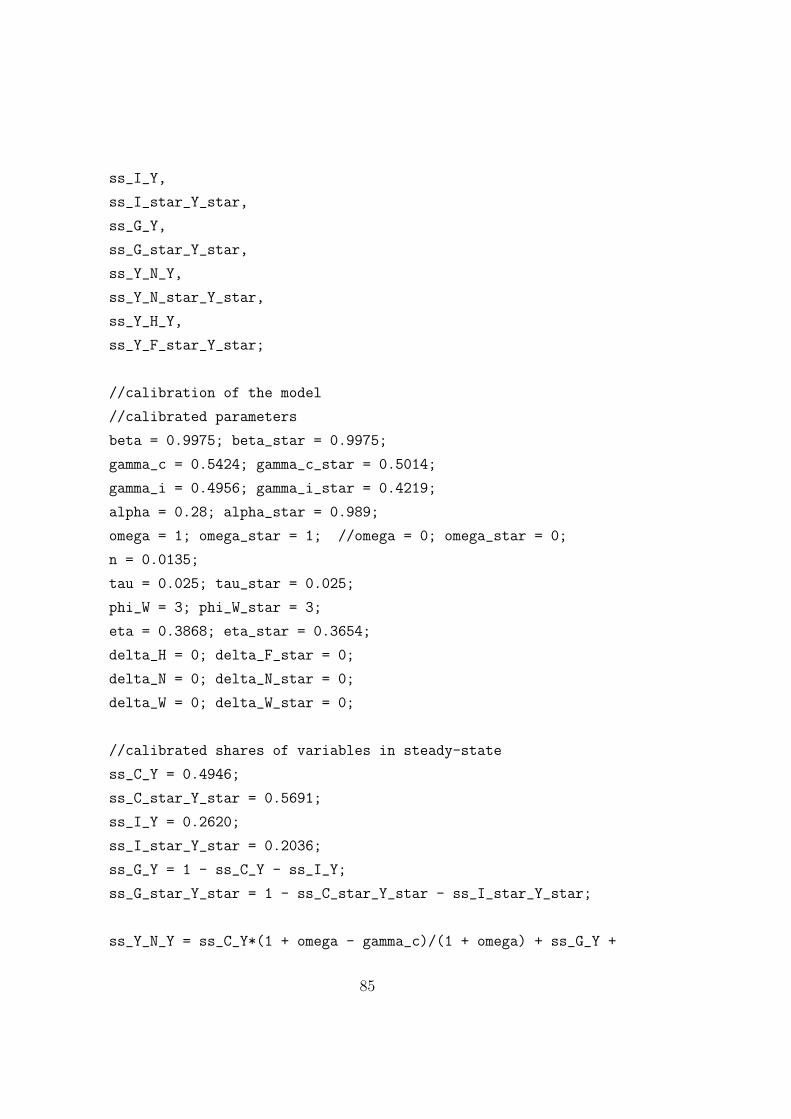
ss_I_Y,
ss_I_star_Y_star,
ss_G_Y,
ss_G_star_Y_star,
ss_Y_N_Y,
ss_Y_N_star_Y_star,
ss_Y_H_Y,
ss_Y_F_star_Y_star;
//calibration of the model
//calibrated parameters
beta = 0.9975; beta_star = 0.9975;
gamma_c = 0.5424; gamma_c_star = 0.5014;
gamma_i = 0.4956; gamma_i_star = 0.4219;
alpha = 0.28; alpha_star = 0.989;
omega = 1; omega_star = 1; //omega = 0; omega_star = 0;
n = 0.0135;
tau = 0.025; tau_star = 0.025;
phi_W = 3; phi_W_star = 3;
eta = 0.3868; eta_star = 0.3654;
delta_H = 0; delta_F_star = 0;
delta_N = 0; delta_N_star = 0;
delta_W = 0; delta_W_star = 0;
//calibrated shares of variables in steady-state
ss_C_Y = 0.4946;
ss_C_star_Y_star = 0.5691;
ss_I_Y = 0.2620;
ss_I_star_Y_star = 0.2036;
ss_G_Y = 1 - ss_C_Y - ss_I_Y;
ss_G_star_Y_star = 1 - ss_C_star_Y_star - ss_I_star_Y_star;
ss_Y_N_Y = ss_C_Y*(1 + omega - gamma_c)/(1 + omega) + ss_G_Y +
85

ss_I_Y*(1 - gamma_i);
ss_Y_N_star_Y_star=ss_C_star_Y_star*(1+omega_star-gamma_c_star)
/(1+omega_star)+ss_G_star_Y_star+ss_I_star_Y_star *
(1 - gamma_i_star);
ss_Y_H_Y = 1 - ss_Y_N_Y;
ss_Y_F_star_Y_star = 1 - ss_Y_N_star_Y_star;
model(linear);
// 1.-6. Market Clearing Conditions
y_H = ss_C_Y/ss_Y_H_Y*gamma_c*alpha/(1+omega)*(c+(1-gamma_c)*x+
(1-alpha)*s)+ss_C_star_Y_star/ss_Y_H_Y*(1-n)/n*gamma_c_star
*(1-alpha_star)/(1+omega_star)*(c_star+(1-gamma_c_star)*
x_star+alpha_star*s) + ss_I_Y/ss_Y_H_Y * gamma_i*alpha *
(i + (1-gamma_i)*(1+omega)*x+(1-alpha)*s)+ss_I_star_Y_star/
ss_Y_H_Y*(1-n)/n*gamma_i_star*(1-alpha_star)*(i_star +
(1-gamma_i_star)*(1+omega_star)*x_star + alpha_star*s);
y_F_star = ss_C_star_Y_star/ss_Y_F_star_Y_star*gamma_c_star*
alpha_star/(1+omega_star)*(c_star+(1-gamma_c_star)*x_star -
(1-alpha_star)*s)+ss_C_Y/ss_Y_F_star_Y_star * n/(1-n) *
gamma_c*(1-alpha)/(1+omega)*(c+(1-gamma_c)*x - alpha*s) +
ss_I_star_Y_star/ss_Y_F_star_Y_star*gamma_i_star*alpha_star
*(i_star + (1-gamma_i_star)*(1+omega_star)*x_star -
(1-alpha_star)*s) + ss_I_Y/ss_Y_F_star_Y_star * n/(1-n) *
gamma_i*(1-alpha) * (i + (1-gamma_i)*(1+omega)*x -alpha*s);
y_N = ss_C_Y/ss_Y_N_Y*((1-gamma_c)*(c-gamma_c*x)+gamma_c*omega/
(1+omega)*(c+(1-gamma_c)*x)) + ss_I_Y/ss_Y_N_Y*(1-gamma_i)*
(i-gamma_i*(1+omega)*x) + ss_G_Y/ss_Y_N_Y * epsilon_g;
86

y_N_star=ss_C_star_Y_star/ss_Y_N_star_Y_star*((1-gamma_c_star)
*(c_star-gamma_c_star*x_star)+gamma_c_star*omega_star/
(1+omega_star)*(c_star+(1-gamma_c_star)*x_star))+
ss_I_star_Y_star/ss_Y_N_star_Y_star*(1-gamma_i_star)*
(i_star-gamma_i_star*(1+omega_star)*x_star)+
ss_G_star_Y_star/ss_Y_N_star_Y_star * epsilon_g_star;
y = ss_Y_H_Y * y_H + ss_Y_N_Y * y_N;
y_star = ss_Y_F_star_Y_star*y_F_star+
ss_Y_N_star_Y_star*y_N_star;
// 7.-8. Euler Equations
c-h*c(-1) = c(+1) - h*c - (1-h)/sigma * (r - pi(+1)) +
(1-h)/sigma * (epsilon_d - epsilon_d(+1));
c_star-h_star*c_star(-1)=c_star(+1)-h_star*c_star-(1-h_star)/
sigma_star*(r_star - pi_star(+1)) + (1-h_star)/sigma_star *
(epsilon_d_star - epsilon_d_star(+1));
// 9. International Risk Sharing Condition
q = epsilon_d_star - epsilon_d - sigma_star/(1-h_star)*
(c_star - h_star * c_star(-1)) + sigma/(1-h)*(c - h*c(-1));
// 10.-11. Law for Capital Acumulation
k = (1-tau)*k(-1) + tau*(i + epsilon_i);
k_star=(1-tau_star)*k_star(-1)+tau_star*(i_star +
epsilon_i_star);
// 12.-13. Real Marginal Costs
r_K = w + l - k(-1);
87

r_K_star = w_star + l_star - k_star(-1);
// 14.-15. Investment Demand
i - i(-1) = beta *(i(+1)-i) + 1/S_prime *(q_T + epsilon_i) -
(gamma_i*(1+omega)-gamma_c)/S_prime * x;
i_star - i_star(-1) = beta_star*(i_star(+1)-i_star)+
1/S_prime_star*(q_T_star+epsilon_i_star)-
(gamma_i_star*(1+omega_star)-gamma_c_star)/
S_prime_star * x_star;
// 16.-17. Price of the Capital
q_T = beta*(1-tau)*q_T(+1)-(r - pi(+1)) +
(1-beta*(1-tau))*r_K(+1);
q_T_star = beta_star *(1-tau_star) * q_T_star(+1) - (r_star -
pi_star(+1)) + (1-beta_star*(1-tau_star))* r_K_star(+1);
// 18.-19. Labor Input
l = eta * (r_K - w) + ss_Y_H_Y * (y_H - epsilon_a_H) +
ss_Y_N_Y * (y_N - epsilon_a_N);
l_star = eta_star * (r_K_star - w_star) + ss_Y_F_star_Y_star *
(y_F_star - epsilon_a_F_star) + ss_Y_N_star_Y_star *
(y_N_star - epsilon_a_N_star);
//20.-21. Real Wage Rate
w-w(-1)=(1-theta_W)*(1-beta*theta_W)/(theta_W*(1+phi_W*phi))*
(mrs-w)+ beta*(w(+1)-w)+beta*(pi(+1)-delta_W*pi) -
(pi - delta_W*pi(-1));
w_star-w_star(-1)=(1-theta_W_star)*(1-beta_star*theta_W_star)/
(theta_W_star*(1+phi_W_star*phi_star))*(mrs_star-w_star)+
88

beta_star*(w_star(+1)-w_star)+beta_star*(pi_star(+1)-
delta_W_star*pi_star)-(pi_star-delta_W_star*pi_star(-1));
//22.-23. Marginal Rate of Substitution
mrs = epsilon_l + phi*l - epsilon_d + sigma/(1-h)*(c-h*c(-1));
mrs_star = epsilon_l_star + phi_star*l_star - epsilon_d_star +
sigma_star/(1-h_star)*(c_star - h_star*c_star(-1));
//24.-25. PC for Raw Tradables
pi_H - delta_H*pi_H(-1) = (1-theta_H)*(1-beta*theta_H)/theta_H*
mc_H+beta *(pi_H(+1) - delta_H*pi_H);
pi_F_star - delta_F_star*pi_F_star(-1) = (1-theta_F_star)*
(1-beta_star*theta_F_star)/theta_F_star * mc_F_star +
beta_star *(pi_F_star(+1) - delta_F_star*pi_F_star);
//26.-27. PC for Non-tradables
pi_N - delta_N*pi_N(-1) = (1-theta_N)*(1-beta*theta_N)/theta_N*
mc_N + beta * (pi_N(+1)- delta_N * pi_N);
pi_N_star-delta_N_star*pi_N_star(-1)=(1-theta_N_star)*
(1-beta_star*theta_N_star)/theta_N_star * mc_N_star +
beta_star * (pi_N_star(+1)- delta_N_star * pi_N_star);
//28.-29. Real Marginal Costs in Tradable Sector
mc_H = (1-eta)*w + eta * r_K - epsilon_a_H + (1-alpha)*s +
(1+omega-gamma_c)*x;
mc_F_star=(1-eta_star)*w_star+eta_star*r_K_star-
epsilon_a_F_star-(1-alpha_star)*s+
(1+omega_star-gamma_c_star)*x_star;
89

//30.-31. Real Marginal Costs in Non-tradable Sector
mc_N = (1-eta)*w + eta * r_K - epsilon_a_N - gamma_c*x;
mc_N_star = (1-eta_star)*w_star + eta_star * r_K_star -
epsilon_a_N_star - gamma_c_star*x_star;
//32.-33. Internal Exchange Rate
x - x(-1) = pi_N - pi_T;
x_star - x_star(-1) = pi_N_star - pi_T_star;
//34.-35. Inflation of Tradables
pi_T = 1/(1+omega)*(pi_H+(1-alpha)*(s-s(-1))+omega*pi_N);
pi_T_star = 1/(1+omega_star)*(pi_F_star-(1-alpha_star)*
(s - s(-1))+omega_star * pi_N_star);
//36.-37. CPI Inflation
pi = gamma_c * pi_T + (1 - gamma_c) * pi_N;
pi_star = gamma_c_star*pi_T_star + (1-gamma_c_star)*pi_N_star;
//38. Real Exchange Rate
q = (alpha + alpha_star-1)*s + (1 + omega_star - gamma_c_star)*
x_star - (1 + omega - gamma_c) * x;
//39.-40. Monetary Policy Rule
r = rho*r(-1)+(1-rho)*(psi_y*y(+1)+psi_pi*pi(+1))+epsilon_m;
r_star=rho_star*r_star(-1)+(1-rho_star)*(psi_y_star*y_star(+1)+
psi_pi_star * pi_star(+1)) + epsilon_m_star;
//41.-42. Productivity Shock in Tradable Sector
90
epsilon_a_H = rho_a_H * epsilon_a_H(-1) + mu_a_H;
epsilon_a_F_star=rho_a_F_star*epsilon_a_F_star(-1)+mu_a_F_star;
//43.-44. Productivity Shock in Non-tradable Sector
epsilon_a_N = rho_a_N * epsilon_a_N(-1) + mu_a_N;
epsilon_a_N_star=rho_a_N_star*epsilon_a_N_star(-1)+mu_a_N_star;
//45.-46. Preference Shock
epsilon_d = rho_d * epsilon_d(-1) + mu_d;
epsilon_d_star=rho_d_star*epsilon_d_star(-1)+mu_d_star;
//47.-48. Labor Supply Shock
epsilon_l = rho_l * epsilon_l(-1) + mu_l;
epsilon_l_star=rho_l_star*epsilon_l_star(-1)+mu_l_star;
//49.-50. Shock in Government Expenditures
epsilon_g = rho_g * epsilon_g(-1) + mu_g;
epsilon_g_star=rho_g_star*epsilon_g_star(-1)+mu_g_star;
//51.-52. Investment Efficiency Shock
epsilon_i = rho_i * epsilon_i(-1) + mu_i;
epsilon_i_star=rho_i_star*epsilon_i_star(-1)+mu_i_star;
//Linking Observables to Model Variables
y_obs = y - y(-1);
y_star_obs = y_star - y_star(-1);
91
pi_obs = pi;
pi_star_obs = pi_star;
x_obs = x - x(-1);
x_star_obs = x_star - x_star(-1);
r_obs = r;
r_star_obs = r_star;
w_obs = w - w(-1);
w_star_obs = w_star - w_star(-1);
c_obs = c - c(-1);
c_star_obs = c_star - c_star(-1);
i_obs = i - i(-1);
i_star_obs = i_star - i_star(-1);
end;
//Model is in the gap form, therefore steady state for all
//variables is 0.
initval;
c = 0; c_star = 0;
x = 0; x_star = 0;
s = 0;
i = 0; i_star = 0;
y_H = 0; y_F_star = 0;
y_N = 0; y_N_star = 0;
y = 0; y_star = 0;
r = 0; r_star = 0;
q = 0;
pi = 0; pi_star = 0;
k = 0; k_star = 0;
92

r_K = 0; r_K_star = 0;
w = 0; w_star = 0;
q_T = 0; q_T_star = 0;
l = 0; l_star = 0;
mrs = 0; mrs_star = 0;
pi_H = 0; pi_F_star = 0;
mc_H = 0; mc_F_star = 0;
pi_N = 0; pi_N_star = 0;
mc_N = 0; mc_N_star = 0;
epsilon_g = 0; epsilon_g_star = 0;
epsilon_d = 0; epsilon_d_star = 0;
epsilon_i = 0; epsilon_i_star = 0;
epsilon_a_H = 0; epsilon_a_F_star = 0;
epsilon_a_N = 0; epsilon_a_N_star = 0;
epsilon_l = 0; epsilon_l_star = 0;
end;
//Estimated Parameters and their Priors
estimated_params;
h, 0.7, 1E-5, 0.9999, beta_pdf,0.7,0.1;
h_star, 0.7, 1E-5, 0.9999, beta_pdf,0.7,0.1;
sigma, 1.0, 1E-5, 10, gamma_pdf,1,0.7;
sigma_star, 1.0, 1E-5, 10, gamma_pdf,1,0.7;
phi, 1.0, 1E-5, 10, gamma_pdf,1,0.7;
phi_star, 1.0, 1E-5, 10, gamma_pdf,1,0.7;
S_prime, 4.0, 1E-5, 10, normal_pdf,4,1.5;
S_prime_star, 4.0, 1E-5, 10, normal_pdf,4,1.5;
//delta_H, 0.5, 1E-5, 0.9999, beta_pdf,0.5,0.2;
//delta_F_star, 0.5, 1E-5, 0.9999, beta_pdf,0.5,0.2;
//delta_N, 0.5, 1E-5, 0.9999, beta_pdf,0.5,0.2;
//delta_N_star, 0.5, 1E-5, 0.9999, beta_pdf,0.5,0.2;
//delta_W, 0.5, 1E-5, 0.9999, beta_pdf,0.5,0.2;
93

//delta_W_star, 0.5, 1E-5, 0.9999, beta_pdf,0.5,0.2;
theta_H, 0.7, 1E-5, 0.9999, beta_pdf,0.7,0.05;
theta_F_star, 0.7, 1E-5, 0.9999, beta_pdf,0.7,0.05;
theta_N, 0.7, 1E-5, 0.9999, beta_pdf,0.7,0.05;
theta_N_star, 0.7, 1E-5, 0.9999, beta_pdf,0.7,0.05;
theta_W, 0.7, 1E-5, 0.9999, beta_pdf,0.7,0.05;
theta_W_star, 0.7, 1E-5, 0.9999, beta_pdf,0.7,0.05;
rho, 0.7, 1E-5, 0.9999, beta_pdf,0.7,0.15;
rho_star, 0.7, 1E-5, 0.9999, beta_pdf,0.7,0.15;
psi_y, 0.25, 1E-5, 2, gamma_pdf,0.25,0.1;
psi_y_star, 0.25, 1E-5, 2, gamma_pdf,0.25,0.1;
psi_pi, 1.3, 1E-5, 5, gamma_pdf,1.3,0.15;
psi_pi_star, 1.3, 1E-5, 5, gamma_pdf,1.3,0.15;
rho_a_H, 0.7, 1E-5, 0.9999, beta_pdf,0.7,0.1;
rho_a_F_star, 0.7, 1E-5, 0.9999, beta_pdf,0.7,0.1;
rho_a_N, 0.7, 1E-5, 0.9999, beta_pdf,0.7,0.1;
rho_a_N_star, 0.7, 1E-5, 0.9999, beta_pdf,0.7,0.1;
rho_d, 0.7, 1E-5, 0.9999, beta_pdf,0.7,0.1;
rho_d_star, 0.7, 1E-5, 0.9999, beta_pdf,0.7,0.1;
rho_l, 0.7, 1E-5, 0.9999, beta_pdf,0.7,0.1;
rho_l_star, 0.7, 1E-5, 0.9999, beta_pdf,0.7,0.1;
rho_g, 0.7, 1E-5, 0.9999, beta_pdf,0.7,0.1;
rho_g_star, 0.7, 1E-5, 0.9999, beta_pdf,0.7,0.1;
rho_i, 0.7, 1E-5, 0.9999, beta_pdf,0.7,0.1;
rho_i_star, 0.7, 1E-5, 0.9999, beta_pdf,0.7,0.1;
stderr mu_a_H, inv_gamma_pdf,2,inf;
stderr mu_a_F_star, inv_gamma_pdf,2,inf;
stderr mu_a_N, inv_gamma_pdf,2,inf;
stderr mu_a_N_star, inv_gamma_pdf,2,inf;
stderr mu_d, inv_gamma_pdf,6,inf;
94

stderr mu_d_star, inv_gamma_pdf,6,inf;
stderr mu_l, inv_gamma_pdf,10,inf;
stderr mu_l_star, inv_gamma_pdf,10,inf;
stderr mu_g, inv_gamma_pdf,3,inf;
stderr mu_g_star, inv_gamma_pdf,3,inf;
stderr mu_i, inv_gamma_pdf,6,inf;
stderr mu_i_star, inv_gamma_pdf,6,inf;
stderr epsilon_m, inv_gamma_pdf,0.3,inf;
stderr epsilon_m_star, inv_gamma_pdf,0.3,inf;
corr mu_a_H, mu_a_F_star, 0, -1, 1, normal_pdf,0,0.4;
corr mu_a_N, mu_a_N_star, 0, -1, 1, normal_pdf,0,0.4;
corr mu_d, mu_d_star, 0, -1, 1, normal_pdf,0,0.4;
corr mu_l, mu_l_star, 0, -1, 1, normal_pdf,0,0.4;
corr mu_g, mu_g_star, 0, -1, 1, normal_pdf,0,0.4;
corr mu_i, mu_i_star, 0, -1, 1, normal_pdf,0,0.4;
corr epsilon_m, epsilon_m_star, 0, -1, 1, normal_pdf,0,0.4;
end;
varobs y_obs, y_star_obs, c_obs, c_star_obs, i_obs,
i_star_obs, r_obs, r_star_obs, pi_obs, pi_star_obs,
w_obs, w_star_obs, x_obs, x_star_obs;
estimation(datafile=data_cz_eu_2Q2000_3Q2011, mh_nblocks=4,
mh_replic=2000000, mh_drop=0.75, mh_jscale=0.25,
mode_check, smoother);
shock_decomposition y_obs y_star_obs c_obs c_star_obs i_obs
i_star_obs r_obs r_star_obs pi_obs pi_star_obs w_obs
w_star_obs x_obs x_star_obs;
95