arX

iv:h

ep-p

h/94

0339

0v1

30

Mar

199

4

BUTP–94/4ROM2F 94/05

hep-ph/9403390

Kl4 - DECAYS BEYOND ONE LOOP♯

J. Bijnensa, G. Colangelob,c and J. Gasserb

September 2018

Abstract

The matrix elements for K → ππlν decays are described by four form fac-tors F,G,H and R. We complete previous calculations by evaluating R atnext-to-leading order in the low-energy expansion. We then estimate higherorder contributions using dispersion relations and determine the low-energyconstants L1, L2 and L3 from data on Ke4 decays and on elastic pion scatter-ing. Finally, we present predictions for the slope of the form factor G and fortotal decay rates.

♯ Work supported in part by Schweizerischer Nationalfonds/ Bundesamt furBildung und Wissenschaft (BBW)/ EEC Human Capital and Mobility Pro-gram/ Fondazione ”Angelo della Riccia”/ INFN.a) NORDITA, Blegdamsvej 17, DK-2100 Copenhagen, Denmark.b) Universitat Bern, Sidlerstrasse 5, CH−3012 Bern, Switzerland.c) Dipartimento di Fisica, Universita di Roma II - ”Tor Vergata”, Via della

Ricerca Scientifica 1, I-00173 Roma, Italy.

1 Introduction

In this article we analyze Kl4 decays,

K → ππlν ; l = e, µ , (1.1)

in the framework of chiral perturbation theory (CHPT). This method, also called”energy expansion” in the following, is based on an expansion of the Green functionsin powers of the external momenta and of the light quark masses [1]-[5]. The matrixelements for Kl4 processes are described by four form factors F,G,H and R. Theirenergy expansion reads

I =MK

Fπ

I(0) + I(2) + I(4) + · · ·

; I = F,G,H,R , (1.2)

where I(n) is a quantity of order En. The predictions for the lowest order terms werefirst given by Weinberg [6]. The anomaly contribution H(2) has been determined in[7], whereas F (2) and G(2) have been evaluated in [8, 9]. For a calculation of H(4)

see [10]. The experimental results [11] for F,G turn out to be 30 − 50% above theleading contributions. The missing piece must then come from higher orders. Theexpressions for F (2), G(2) involve the low-energy constants L1, . . . , L9, which are notfixed by chiral symmetry alone and which must be determined phenomenologicallyat the present stage of our capability to solve QCD. This was done in [3], wherethe Li’s were pinned down using experimental data (not related to Kl4 decays)and involving the large-NC prediction which states that, in the limit where thenumber of colors becomes large, certain combinations of the low-energy constantsare suppressed. The decay (1.1) is the simplest process where this rule can be tested[8, 9]. In addition, it allows one to perform an independent determination of L1, L2

and L3 and thus to check consistency with other data.The aim of the present article is threefold. First, we fill the gap in the literature

and evaluate also the next-to-leading order term R(2). [The amplitude R is com-pletely negligible in Ke4 decays, because its contribution to the rate is suppressed bythe factor m2

l . It must be retained, however, in the Kµ4 channel ]. Second, we notethat, because the strange quark mass is not very small on a typical hadronic scale,the corrections I(2) to the leading-order terms of the form factors are substantial.The determination of the Li’s from Kl4 decays is therefore affected with substantialuncertainties if carried out using only the first two terms in the expansion (1.2),as was done in [8, 9]. Here we improve these calculations by estimating the size ofhigher order contributions to F . We use for this purpose the method developed in[12], which amounts to write a dispersive representation for the relevant partial waveamplitudes, fixing the corresponding subtraction constants with chiral perturbationtheory. We are then able to reduce the uncertainties in the determination of L1, L2

and L3 in a significant manner, even more so if data on elastic ππ scattering isconsidered in addition. Third, we predict the slope of the form factor G, and showthat we may evaluate total decay rates for all channels in Kl4 decays within rather

2

small uncertainties, provided the leading S- and P - wave form factors have beendetermined experimentally e.g. from K+ → π+π−e+νe decays.

The plan of the paper is as follows. In section 2, we provide the necessarykinematics and the definition of the form factors. Section 3 contains the result ofthe one-loop calculation of these quantities. In section 4, we use dispersion relationsto construct a I = 0 S-wave amplitude which has the correct phase to higherorders in the low-energy expansion. In section 5, we use this improved amplitude todetermine the low-energy constants L1, L2 and L3. Section 6 contains predictions,whereas a summary and concluding remarks are presented in section 7.

2 Kinematics and form factors

We discuss the decays

K+(p) → π+(p1) π−(p2) l

+(pl) νl(pν) , (2.1)

K+(p) → π0(p1) π0(p2) l

+(pl) νl(pν) , (2.2)

K0(p) → π0(p1) π−(p2) l

+(pl) νl(pν) ; l = e, µ , (2.3)

and their charge conjugate modes. We do not consider isospin violating contributionsand correspondingly set mu = md, αQED = 0.

2.1 Kinematics

We start with the process (2.1). The full kinematics of this decay requires fivevariables. We will use the ones introduced by Cabibbo and Maksymowicz [13]. It isconvenient to consider three reference frames, namely the K+ rest system (ΣK), theπ+π− center-of-mass system (Σ2π) and the l+νl center-of-mass system (Σlν). Thenthe variables are

1. sπ, the effective mass squared of the dipion system,

2. sl, the effective mass squared of the dilepton system,

3. θπ, the angle of the π+ in Σ2π with respect to the dipion line of flight in ΣK ,

4. θl, the angle of the l+ in Σlν with respect to the dilepton line of flight in ΣK ,and

5. φ, the angle between the plane formed by the pions in ΣK and the correspond-ing plane formed by the dileptons.

The angles θπ, θl and φ are displayed in Fig. 1.

3

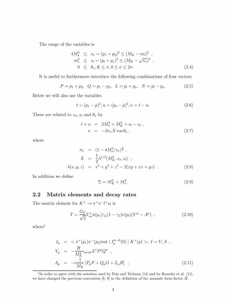
The range of the variables is

4M2π ≤ sπ = (p1 + p2)

2 ≤ (MK −ml)2 ,

m2l ≤ sl = (pl + pν)

2 ≤ (MK −√sπ)

2 ,

0 ≤ θπ, θl ≤ π, 0 ≤ φ ≤ 2π. (2.4)

It is useful to furthermore introduce the following combinations of four vectors

P = p1 + p2, Q = p1 − p2, L = pl + pν , N = pl − pν . (2.5)

Below we will also use the variables

t = (p1 − p)2, u = (p2 − p)2, ν = t− u. (2.6)

These are related to sπ, sl and θπ by

t + u = 2M2π +M2

K + sl − sπ ,

ν = −2σπX cos θπ , (2.7)

where

σπ = (1− 4M2π/sπ)

12 ,

X =1

2λ1/2(M2

K , sπ, sl) ,

λ(x, y, z) = x2 + y2 + z2 − 2(xy + xz + yz) . (2.8)

In addition we defineΣ = M2

K +M2π . (2.9)

2.2 Matrix elements and decay rates

The matrix element for K+ → π+π−l+νl is

T =GF√2V ⋆usu(pν)γµ(1− γ5)ν(pl)(V

µ − Aµ) , (2.10)

where1

Iµ = < π+(p1)π−(p2)out | I4−i5

µ (0) | K+(p) >; I = V,A ,

Vµ = − H

M3K

ǫµνρσLνP ρQσ ,

Aµ = −i1

MK[PµF +QµG+ LµR] , (2.11)

1In order to agree with the notation used by Pais and Treiman [14] and by Rosselet et al. [11],we have changed the previous convention [8, 9] in the definition of the anomaly form factor H .

4

and ǫ0123 = 1. The matrix elements for the other channels (2.2, 2.3) may be obtainedfrom (2.10, 2.11) by isospin symmetry, see below.

The form factors F,G,R and H are analytic functions of the variables sπ, t andu. The partial decay rate for (2.1) is given by

dΓ =1

2MK(2π)8∑

spins

| T |2 δ4(p− P − L)d3p12p01

d3p22p02

d3pl2p0l

d3pν2p0ν

. (2.12)

The quantity∑

spins | T |2 is a Lorentz invariant quadratic form in F,G,R andH . All scalar products can be expressed in terms of the 5 independent variablessπ, sl, θπ, θl and φ, such that

∑

spins

| T |2= 2G2F | Vus |2M−2

K J5(sπ, sl, θπ, θl, φ) . (2.13)

Carrying out the integrations over the remaining 4 · 3 − 5 = 7 variables in (2.12)gives [13]

dΓ5 = G2F | Vus |2 N(sπ, sl)J5(sπ, sl, θπ, θl, φ)dsπdsld(cos θπ)d(cos θl)dφ ,

N(sπ, sl) = (1− zl)σπX/(213π6M5K) , (2.14)

where

J5 = 2(1− zl)[

I1 + I2 cos 2θl + I3 sin2 θl · cos 2φ+ I4 sin 2θl · cos φ

+ I5 sin θl · cosφ+ I6 cos θl + I7 sin θl · sinφ+ I8 sin 2θl · sin φ+ I9 sin

2 θl · sin 2φ]

,

with

I1 =1

4

(1 + zl)|F1|2 +1

2(3 + zl)

(

|F2|2 + |F3|2)

sin2 θπ + 2zl|F4|2

,

I2 = −1

4(1− zl)

|F1|2 −1

2

(

|F2|2 + |F3|2)

sin2 θπ

,

I3 = −1

4(1− zl)

|F2|2 − |F3|2

sin2 θπ ,

I4 =1

2(1− zl) Re(F

∗

1F2) sin θπ ,

I5 = − Re(F ∗

1F3) + zl Re(F∗

4F2) sin θπ ,

I6 = −

Re(F ∗

2F3) sin2 θπ − zl Re(F

∗

1F4)

,

I7 = − Im(F ∗

1F2) + zl Im(F ∗

4F3) sin θπ ,

I8 =1

2(1− zl) Im(F ∗

1F3) sin θπ ,

I9 = −1

2(1− zl) Im(F ∗

2F3) sin2 θπ , (2.15)

5

and

F1 = X · F + σπ(PL) cos θπ ·G ,

F2 = σπ (sπsl)1/2G ,

F3 = σπX (sπsl)1/2 H

M2K

,

F4 = −(PL)F − slR − σπX cos θπ ·G . (2.16)

The definition of F1, . . . , F4 corresponds to the combinations used by Pais andTreiman [14] (the different sign in the terms ∼ PL is due to our use of the metricdiag(+−−−)). The form factors I1, . . . , I9 agree with the expressions given in [14].

2.3 Isospin decomposition

The Kl4 decays (2.2) and (2.3) involve the same form factors as displayed in Eq.(2.11). We denote by A+−, A00 and A0− the current matrix elements of the processes(2.1)-(2.3). They are related by isospin symmetry2,

A+− =A0−√

2−A00 . (2.17)

This relation also holds for the individual form factors, which may be decomposedinto a symmetric and an antisymmetric part under t ↔ u (p1 ↔ p2). Because ofBose symmetry and of the ∆I = 1

2rule of the relevant weak currents, one has

(F,G,R,H)00 = −(F+, G−, R+, H−)+− ,

(F,G,R,H)0− =√2(F−, G+, R−, H+)+− , (2.18)

where

F±

+−=

1

2[F (sπ, t, u)± F (sπ, u, t)] , (2.19)

and F (sπ, t, u) is defined in Eq. (2.11). G±, R± and H± are defined similarly. Theisospin relation for the decay rates is

Γ(K+ → π+π−l+νl) =1

2Γ(K0 → π0π−l+νl) + 2Γ(K+ → π0π0l+νl) . (2.20)

2.4 Partial wave expansion

The form factors may be written in a partial wave expansion in the variable θπ. Weconsider a definite isospin ππ state. Suppressing isospin indices, one has [15]

F =∞∑

l=0

Pl(cos θπ)fl −σπPL

Xcos θπG ,

2We use the Condon-Shortley phase conventions. Notice that we evaluate matrix elements anddecay rates for K0 – they differ from the corresponding KL-quantities by a normalization factor.

6

G =∞∑

l=1

P ′

l (cos θπ)gl ,

R =∞∑

l=0

Pl(cos θπ)rl +σπsπX

cos θπG ,

H =∞∑

l=0

P ′

l (cos θπ)hl , (2.21)

where

P ′

l (z) =d

dzPl(z) . (2.22)

The partial wave amplitudes fl, gl, rl and hl depend on sπ and sl. Their phasecoincides with the phase shifts δIl in elastic ππ scattering (angular momentum l,isospin I). More precisely, the quantities

e−iδ02lX2l ,

e−iδ12l+1X2l+1 ; l = 0, 1, . . . ; X = f, g, r, h , (2.23)

are real in the physical region of Kl4 decay (in our overall phase convention). Theform factors F1 and F4 therefore have a simple expansion,

F1 = X∑

l

Pl(cos θπ)fl ,

F4 = −∑

l

Pl(cos θπ)(PLfl + slrl). (2.24)

3 Theory

The theoretical predictions of Kl4 form factors have a long history which startedin the sixties with the current algebra evaluation of F , G, R and H . For an earlyreview of the subject and for references to work prior to CHPT we refer the readerto [16] (see also [17]). Here we concentrate on the evaluation of the form factors inthe framework of CHPT [8, 9, 18].

3.1 Tree level

The chiral representation of the form factors at leading order was originally givenby Weinberg [6],

F = G =MK√2Fπ

= 3.74 ,

R =MK

2√2Fπ

(

sπ + ν

sl −M2K

+ 1

)

,

H = 0 . (3.1)

7

The next-to-leading order corrections are displayed below, and the later sectionscontain an estimate of yet higher order contributions. Here we note that the totaldecay rates which follow from Eq. (3.1) are typically a factor of two (ore more)below the data. As an example, consider the channel K+ → π+π−e+νe. Using(3.1), the total decay rate becomes3 1297 sec−1, whereas the experimental value is3160±140 sec−1 [32].

3.2 The form factors at one-loop

In Ref. [8, 9], the form factors F , G and H have been evaluated in CHPT at orderp4 (see also [19]). We complement these works with the evaluation of R at the sameorder. Below we display the result of our calculation, referring the reader to theabove references and to available reviews [5] for the details of the methods used.

In order to make this article reasonably self-contained, we display the result ofall four form factors. The result for F may be written in the form

F (sπ, t, u) =MK√2Fπ

1 +1

F 2π

(UF + PF + CF ) +O(E4)

. (3.2)

The contribution UF (sπ, t, u) denotes the unitarity correction generated by the one-loop graphs which appear at order E4 in the low-energy expansion. It has the form

UF (sπ, t, u) = ∆0(sπ) + AF (t) +B(t, u) , (3.3)

with

∆0(sπ) =1

2(2sπ −M2

π)Jrππ(sπ) +

3sπ4

JrKK(sπ) +

M2π

2Jrηη(sπ) ,

AF (t) =1

16

[

(14M2K + 14M2

π − 19t)JrKπ(t) + (2M2

K + 2M2π − 3t)Jr

ηK(t)]

+1

8

[

(3M2K − 7M2

π + 5t)KKπ(t) + (M2K − 5M2

π + 3t)KηK(t)]

− 1

4

[

9(LKπ(t) + LηK(t)) + (3M2K − 3M2

π − 9t)(M rKπ(t) +M r

ηK(t))]

,

B(t, u) = −1

2(M2

K +M2π − t)Jr

Kπ(t)− (t ↔ u). (3.4)

The loop integrals Jrππ(sπ), . . . which occur in these expressions are listed in appendix

A. The functions JrPQ and M r

PQ depend on the scale µ at which the loops arerenormalized. The scale drops out in the expression for the full amplitude (seebelow).

The imaginary part of F−2π ∆0(sπ) contains the I = 0, S-wave ππ phase shift

δ00(sπ) = (32πF 2π )

−1(2sπ −M2π)σπ +O(E4) , (3.5)

3If not stated otherwise, we use Fπ = 93.2 MeV, |Vus| = 0.22 and (Mπ,MK) = (139.6, 493.6)MeV, (135, 493.6) MeV and (137, 497.7) Mev for the decays (2.1), (2.2) and (2.3), respectively.

8

as well as contributions from KK and ηη intermediate states. The functions AF (t)and B(t, u) are real in the physical region.

The contribution PF (sπ, t, u) is a polynomial in sπ, t, u obtained from the treegraphs at order E4. We find

PF (sπ, t, u) =9∑

i=1

pi,F (sπ, t, u)Lri , (3.6)

where

p1,F = 32(sπ − 2M2π) ,

p2,F = 8(M2K + sπ − sl) ,

p3,F = 4(M2K − 3M2

π + 2sπ − t) ,

p4,F = 32M2π ,

p5,F = 4M2π ,

p9,F = 2sl . (3.7)

The remaining coefficients pi,F are zero. The quantities Lri denote the renormalized

coupling constants which parametrize the effective lagrangian at order E4 [3]. Theirscale dependence is

Lri (µ2) = Lr

i (µ1) +Γi

16π2ln

µ1

µ2. (3.8)

Observable quantities are independent of the scale µ, once the loop contributionsare included. The coefficients Γi are displayed in table 1, together with the value [3]of the couplings Lr

i at µ = Mρ.The contributions CF contain logarithmic terms, independent of sπ, t and u:

CF =1

256π2

[

5M2π ln

M2π

µ2− 2M2

K lnM2

K

µ2− 3M2

η lnM2

η

µ2

]

. (3.9)

The corresponding decomposition of the form factor G is

G(sπ, t, u) =MK√2Fπ

1 +1

F 2π

(UG + PG + CG) +O(E4)

,

UG(sπ, t, u) = ∆1(sπ) + AG(t) +B(t, u) , (3.10)

with

∆1(sπ) = 2sπ

M rππ(sπ) +

1

2M r

KK(sπ)

,

AG(t) =1

16

[

(2M2K + 2M2

π + 3t)JrKπ(t)− (2M2

K + 2M2π − 3t)Jr

ηK(t)]

+1

8

[

(−3M2K + 7M2

π − 5t)KKπ(t) + (−M2K + 5M2

π − 3t)KηK(t)]

− 3

4

[

LKπ(t) + LηK(t)− (M2K −M2

π + t)(M rKπ(t) +M r

ηK(t))]

.

(3.11)

9

Table 1: Phenomenological values and source for the renormalized coupling con-stants Lr

i (Mρ) according to Ref. [3]. The quantities Γi in the fourth column deter-mine the scale dependence of the Lr

i (µ) according to Eq. (3.8). Lr11 and Lr

12 are notdirectly accessible to experiment.

i Lri (Mρ)× 103 source Γi

1 0.7 ± 0.5 ππ D-waves, Zweig rule 3/322 1.3 ± 0.7 ππ D-waves 3/163 −4.4 ± 2.5 ππ D-waves, Zweig rule 04 −0.3 ± 0.5 Zweig rule 1/85 1.4 ± 0.5 FK : Fπ 3/86 −0.2 ± 0.3 Zweig rule 11/1447 −0.4 ± 0.2 Gell-Mann-Okubo,L5, L8 08 0.9 ± 0.3 MK0 −MK+, L5, 5/48

(2ms −mu −md) : (md −mu)

9 6.9 ± 0.7 < r2 >πem 1/4

10 −5.5 ± 0.7 π → eνγ − 1/411 −1/812 5/24

The imaginary part of F−2π ∆1(sπ) contains the I = 1, P -wave phase shift

δ11(sπ) = (96πF 2π )

−1sπσ3π +O(E4) . (3.12)

as well as contributions from KK intermediate states. The function AG is real inthe physical region.

The polynomials

PG =9∑

i=1

pi,G(sπ, t, u)Lri (3.13)

are

p2,G = 8(t− u) ,

p3,G = 4(t−M2K −M2

π) ,

p5,G = 4M2π ,

p9,G = 2sl ,

(3.14)

The remaining pi,G vanish. The logarithms contained in CG are

CG = −CF . (3.15)

The form factor R contains a pole part Z(sπ, t, u)/(sl−M2K) and a regular piece

Q. [Since the axial current acts as an interpolating field for a kaon, the residue of

10

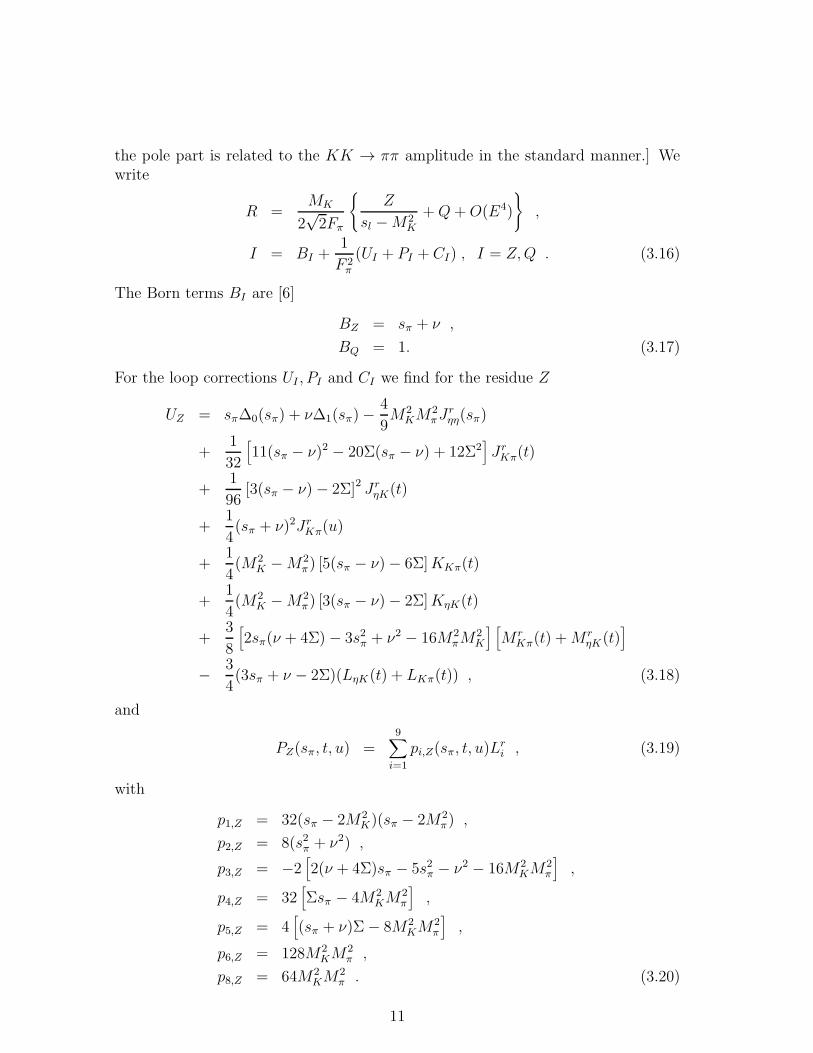
the pole part is related to the KK → ππ amplitude in the standard manner.] Wewrite

R =MK

2√2Fπ

Z

sl −M2K

+Q+O(E4)

,

I = BI +1

F 2π

(UI + PI + CI) , I = Z,Q . (3.16)

The Born terms BI are [6]

BZ = sπ + ν ,

BQ = 1. (3.17)

For the loop corrections UI , PI and CI we find for the residue Z

UZ = sπ∆0(sπ) + ν∆1(sπ)−4

9M2

KM2πJ

rηη(sπ)

+1

32

[

11(sπ − ν)2 − 20Σ(sπ − ν) + 12Σ2]

JrKπ(t)

+1

96[3(sπ − ν)− 2Σ]2 Jr

ηK(t)

+1

4(sπ + ν)2Jr

Kπ(u)

+1

4(M2

K −M2π) [5(sπ − ν)− 6Σ]KKπ(t)

+1

4(M2

K −M2π) [3(sπ − ν)− 2Σ]KηK(t)

+3

8

[

2sπ(ν + 4Σ)− 3s2π + ν2 − 16M2πM

2K

] [

M rKπ(t) +M r

ηK(t)]

− 3

4(3sπ + ν − 2Σ)(LηK(t) + LKπ(t)) , (3.18)

and

PZ(sπ, t, u) =9∑

i=1

pi,Z(sπ, t, u)Lri , (3.19)

with

p1,Z = 32(sπ − 2M2K)(sπ − 2M2

π) ,

p2,Z = 8(s2π + ν2) ,

p3,Z = −2[

2(ν + 4Σ)sπ − 5s2π − ν2 − 16M2KM

2π

]

,

p4,Z = 32[

Σsπ − 4M2KM

2π

]

,

p5,Z = 4[

(sπ + ν)Σ− 8M2KM

2π

]

,

p6,Z = 128M2KM

2π ,

p8,Z = 64M2KM

2π . (3.20)

11

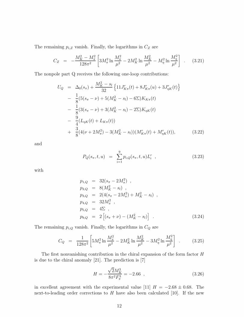
The remaining pi,Z vanish. Finally, the logarithms in CZ are

CZ = −M2K −M2

π

128π2

[

3M2π ln

M2π

µ2− 2M2

K lnM2

K

µ2−M2

η lnM2

η

µ2

]

. (3.21)

The nonpole part Q receives the following one-loop contributions:

UQ = ∆0(sπ) +M2

K − sl32

11JrKπ(t) + 8Jr

Kπ(u) + 3JrηK(t)

− 1

8(5(sπ − ν) + 5(M2

K − sl)− 6Σ)KKπ(t)

− 1

8(3(sπ − ν) + 3(M2

K − sl)− 2Σ)KηK(t)

− 9

4(LηK(t) + LKπ(t))

+3

8(4(ν + 2M2

π)− 3(M2K − sl))(M

rKπ(t) +M r

ηK(t)), (3.22)

and

PQ(sπ, t, u) =9∑

i=1

pi,Q(sπ, t, u)Lri , (3.23)

with

p1,Q = 32(sπ − 2M2π) ,

p2,Q = 8(M2K − sl) ,

p3,Q = 2(4(sπ − 2M2π) +M2

K − sl) ,

p4,Q = 32M2π ,

p5,Q = 4Σ ,

p9,Q = 2[

(sπ + ν)− (M2K − sl)

]

. (3.24)

The remaining pi,Q vanish. Finally, the logarithms in CQ are

CQ =1

128π2

[

5M2π ln

M2π

µ2− 2M2

K lnM2

K

µ2− 3M2

η lnM2

η

µ2

]

. (3.25)

The first nonvanishing contribution in the chiral expansion of the form factor His due to the chiral anomaly [21]. The prediction is [7]

H = −√2M3

K

8π2F 3π

= −2.66 , (3.26)

in excellent agreement with the experimental value [11] H = −2.68 ± 0.68. Thenext-to-leading order corrections to H have also been calculated [10]. If the new

12

low-energy parameters are estimated using the vector-mesons only, these correctionsare small.

The results for F,G and R must satisfy two nontrivial constraints: i) Unitarityrequires that F,G and R contain, in the physical region 4M2

π ≤ sπ ≤ (MK −ml)2,

imaginary parts governed by S- and P -wave ππ scattering [these imaginary partsare contained in the functions ∆0(sπ),∆1(sπ)]. ii) The scale dependence of the low-energy constants Lr

i must be compensated by the scale dependence of UF,G,Z,Q andCF,G,Z,Q for all values of sπ, t, u,M

2π ,M

2K . [Since we work at order E4 in the chiral

expansion, the meson masses appearing in the above expressions satisfy the Gell-Mann-Okubo mass formula.] We have checked that these constraints are satisfied.

It is one of the aims of this article to determine the low-energy constants Lr1, L

r2

and L3 from experimental data on K+ → π+π−e+νe decays and on ππ thresholdparameters. In Ref. [8, 9], the above one-loop expressions have been used for thispurpose. Because the one-loop contributions are rather large, the values of theLi’s so extracted suffer from substantial uncertainties. In the following section, wetherefore first estimate the effects from higher orders in the chiral expansion, usingthen this improved representation for the form factors in a comparison with thedata.

4 Beyond one-loop

To investigate the importance of higher order terms, we employ the method devel-oped in Ref. [12]. It amounts to writing a dispersive representation of the partialwave amplitudes, fixing the subtraction constants using chiral perturbation theory.Here, we estimate the higher order terms in the S-wave projection of the amplitudeF1,

f(sπ, sl) = (4πX)−1∫

dΩF1(sπ, t, sl) , (4.1)

because this form factor plays a decisive role in the determination of Lr1, L

r2 and L3,

and it is influenced by S-wave ππ scattering which is known [22, 23] to producesubstantial corrections.

4.1 Analytic properties of f(sπ, sl)

Only the crossing even part

F+1 = XF+ + σπ(PL) cos θπ ·G− (4.2)

contributes in the projection (4.1). The partial wave f has the following analyticproperties:

1. At fixed sl, it is analytic in the complex sπ-plane, cut along the real axis forRe sπ ≥ 4M2

π and Re sπ ≤ 0.

2. In the interval 0 ≤ sπ ≤ 4M2π , it is real.

13

3. In 4M2π ≤ sπ ≤ 16M2

π , its phase coincides with the isospin zero S-wave phaseδ00 in elastic ππ scattering,

f+ = e2iδ00f− , f± = f(sπ ± iǫ, sl). (4.3)

The proof of these properties is standard [24]. Here we only note that the presenceof the cut for sπ ≤ 0 follows from the relations

t = M2π +

M2K + sl − sπ

2− σπX cos θπ ,

t(cos θπ = −1, sπ < 0) ≥ (MK +Mπ)2. (4.4)

Since F+ and G− have cuts at t ≥ (MK +Mπ)2 [see e.g. Eqs. 3.2–3.11], the claim

is proven.

4.2 Unitarization

We introduce the Omnes-function

Ω(sπ) = exp

[

sππ

∫ Λ2

4M2π

ds

s

δ00(s)

s− sπ

]

, (4.5)

where Λ will be chosen of the order of 1 GeV below. According to (4.3), multiplica-tion by Ω−1 removes the cut in f for 4M2

π ≤ sπ ≤ 16M2π . Consider now

f = fL + fR , (4.6)

where fL(fR) has only the left-hand (right-hand) cut, and introduce

v = Ω−1(f − fL) . (4.7)

Then v has only a right-hand cut, and we may represent it in a dispersive way,

v = v0 + v1sπ +s2ππ

∫

∞

4M2π

ds

s2ImΩ−1(f − fL)

s− sπ. (4.8)

We expect the contributions from the integral beyond 1GeV2 to be small. Further-more, Ω−1f is approximately real between 16M2

π and 1GeV2, as a result of whichone has

v = v0 + v1sπ −s2ππ

∫ Λ2

4M2π

ds

s2fLImΩ−1

s− sπ. (4.9)

For given v0, v1, fL and Ω, the form factor f is finally obtained from

f = fL + Ωv . (4.10)

The behaviour of fL at sπ → 0 is governed by the large |t|-behaviour of F+ andG−, see (4.4). Therefore, instead of using CHPT to model fL, we approximate the

14

left-hand cut by resonance exchange. To pin down the subtraction constants v0 andv1, we require that the threshold expansion of f and fCHPT agree up to and includingterms of order O(E2). For a specific choice of fL, this fixes v0, v1 in terms of thequantities which occur in the one-loop representation of F+ and G−. In the casewhere fL = 0, f has then a particularly simple form at sl = 0,

f(sπ, sl = 0)|fL=0 = Ω(v0 + v1sπ) ,

v0 =MK√2Fπ

1.05 +1

F 2π

[

− 64M2πL

r1 + 8M2

KLr2

+2(M2K − 8M2

π)L3 +2

3(M2

K − 4M2π)(4L

r2 + L3)

]

,

v1 =MK√2Fπ

0.38 +1

F 2π

[

32Lr1 + 8Lr

2 + 10L3

−2

3

M2K − 4M2

π

4M2π

(4Lr2 + L3)

]

. (4.11)

We relegate the details of the calculation of fL, v0 and of v1 to appendix C.In the partial wave f , the effects of the final-state interactions are substantial,

because they are related to the I = 0, S-wave ππ phase shift. On the other hand,for the leading partial wave in G+ = geiδp + · · ·, these effects are reduced, becausethe phase δp is small at low energies. We find it more difficult to assess an estimatefor the higher order corrections in this case – we come back to this point in thefollowing section.

5 Determination of L1, L2 and L3

Here we determine the low-energy constants Lr1, L

r2 and L3 from experimental data

on K+ → π+π−e+νe decays and on ππ → ππ threshold parameters, using theimproved S-wave amplitude f set up above. We are aware that our results will notbe the last word: future kaon facilities like DAΦNE [20] will allow a more refinedcomparison of the chiral representation with the data. Nevertheless, we believe thatit is instructive to see what one has to expect from higher order contributions. Acomparison with earlier work [9] will be provided at the end of this section.

5.1 The data

Experimentally the study of Kl4 decays is dominated by the work of Rosselet et al.[11] which measures K+ → π+π−e+νe with good statistics. The total decay rate,the absolute value of the form factors F,G and of H and the difference of the phasesδ00 − δ11 were determined by use of

F = fseiδs + fpe

iδp cos θπ +D − wave ,

G = geiδp +D − wave ,

H = heiδh +D − wave . (5.1)

15

The form factor fp was found to be compatible with zero and hence set equal tozero when the final value for g was derived. No sπ, sl dependence of the ratios g/fsand h/fs was seen. Parametrizing fs in the form

fs = fs(0)(1 + λfq2) ,

q2 = (sπ − 4M2π)/4M

2π , (5.2)

then gives

g = g(0)(1 + λgq2) ,

h = h(0)(1 + λhq2) , (5.3)

with λf = λg = λh. Rosselet et al. found [11]

fs(0) = 5.59± 0.14 ,g(0) = 4.77± 0.27 ,h(0) = −2.68± 0.68 ,λf = 0.08± 0.02 ,

(5.4)

where we have used |Vus| = 0.22 in transcribing their results. Notice that the exper-imental numbers (5.4) have been obtained in [11] under assumptions which are inconflict with our theoretical formulae, like absence of higher waves, sl independenceof the form factors and equality of the slopes, λf = λg = λh. It would of course bedesirable to analyze forthcoming data without any additional assumptions.

The total decay rate is [11]

ΓKe4= (3.26± 0.15)103sec−1 . (5.5)

In [9] it has been observed that, using as input the central values (5.4), one obtainsΓKe4

= 2.94·103 sec−1, which disagrees with (5.5). On the other hand, the value (5.5)was used in Ref. [11] to normalize the form factors in (5.4). We do not understandthe origin of this contradiction.

The ππ threshold data used below are taken from Ref. [25]. We display them intable 2, column 6.

5.2 The fits

In the following, we perform various fits to fs(0), λf , g(0) and to the ππ thresholdparameters listed in table 2. We introduce for this purpose the quantities

f(sπ, sl) =

∣

∣

∣

∣

(4πX)−1∫

dΩF1(sπ, t, sl)

∣

∣

∣

∣

= |f(sπ, sl)| ,

g(sπ, sl) =∣

∣

∣

∣

3

8π

∫

dΩ sin2 θπG(sπ, t, sl)∣

∣

∣

∣

, (5.6)

16

Table 2: Results of fits with one-loop and unitarized form factors, respectively. Theerrors quoted for the Lr

i ’s are statistical only. The Lri are given in units of 10−3 at

the scale µ = Mρ, the scattering lengths aIl and the slopes bIl in appropriate powersof Mπ+ .

Ke4 data alone Ke4 and ππ data experimentone-loop unitarized one-loop unitarized [25]

Lr1 0.65± 0.27 0.36± 0.26 0.60± 0.24 0.37± 0.23

Lr2 1.63± 0.28 1.35± 0.27 1.50± 0.23 1.35± 0.23

L3 −3.4± 1.0 −3.4 ± 1.0 −3.3± 0.86 −3.5 ± 0.85a00 0.20 0.20 0.20 0.20 0.26± 0.05b00 0.26 0.25 0.26 0.25 0.25± 0.03

−10 a20 0.40 0.41 0.40 0.41 0.28± 0.12−10 b20 0.67 0.72 0.68 0.72 0.82± 0.0810a11 0.36 0.37 0.36 0.37 0.38± 0.02102b11 0.44 0.47 0.43 0.48102a02 0.22 0.18 0.21 0.18 0.17± 0.03103a22 0.39 0.21 0.37 0.20 0.13± 0.3

χ2/NDOF 0/0 0/0 8.8/7 4.9/7

where the factor 3/2 sin2 θ appears because G is expanded in derivatives of Legendrepolynomials. Below, we confront [fs(0), g(0)] with [f(4M2

π , sl)], g(4M2π , sl)], which

depend on sl. Furthermore, we compare the slope λf with

λf(sπ, sl) =f(sπ, sl)− f(4M2

π , sl)

f(4M2π , sl)

4M2π

sπ − 4M2π

, (5.7)

which depends on both sπ and sl. Below we use these dependences to estimatesystematic uncertainties in the determination of the low-energy couplings. [In futurehigh statistics experiments, the sl-dependence of the form factors will presumablybe resolved. It will be easy to adapt the procedure to this case.]

We have used MINUIT [26] to perform the fits. The results for the choice sl =0, sπ = 4.4M2

π are given in table 2. In the columns denoted by ”one-loop”, we haveevaluated f , g and λf from the one-loop representation given above4. In the fitwith the unitarized form factor (columns 3 and 5), we have evaluated f from Eqs.(4.10,C.1), inserting in the Omnes function the parametrization of the ππ S-wavephase shift proposed by Schenk [27, solution B]. For the form factor G, we haveagain used the one-loop representation. The statistical errors quoted for the Li’sare the ones generated by the procedure MINOS in MINUIT and correspond to anincrease of χ2 by one unit.

A few remarks are in order at this place.

4We always use for Lr

4, . . . , Lr

9the values quoted in table 1.

17

1. It is seen that the overall description of the ππ scattering data is better usingthe unitarized form factors, in particular so for the D-wave scattering lengths.

2. The errors quoted do not give account of the fact that the simultaneous deter-mination of the three constants produces a strong correlation between them.To illustrate this point we note that, while the values of the Li’s in column 4and 5 are apparently consistent with each other within one error bar, the χ2

in column 5 increases from 4.9 to 30.7 if the Li’s from column 4 are used inthe evaluation of χ2 in column 5. (For a discussion about the interpretationof the errors see [26]).

3. The low-energy constants l1, l2 which occur in SU(2)L×SU(2)R analyses maybe evaluated from a given set of Lr

1, Lr2 and L3 [3]. Their value changes in

a significant way by using the unitarized amplitude instead of the one-loopformulae: the values for (l1, l2) in column 4 and 5 are (−0.5± 0.88, 6.4± 0.44)and (−1.7± 0.85, 6.0± 0.4), respectively.

4. Lr1, L

r2 and L3 are related to ππ phase-shifts through sum rules [28, 29]. In

principle, one should take these constraints into account as well5. We do notconsider them here, because we find it very difficult to assess a reliable errorfor the integrals over the total ππ cross sections which occur in those relations.

The statistical error in the data is only one source of the uncertainty in the low-energy constants, which are in addition affected by the ambiguities in the estimateof the higher order corrections. These systematic uncertainties have several sources:

i) Higher order corrections to g have not been taken into account.

ii) The determination of the contribution from the left-hand cut is not unique.

iii) The quantities f and g depend on sl, and λf is a function of both sl and sπ.

iv) The Omnes function depends on the elastic ππ phase shift and on the cutoffΛ used.

We have considered carefully these effects. As for the first point, we have evalu-ated the higher orders in g in two ways:

• We define the quantity [9]

∆g =(g(0)− g(2))2

g(2), (5.8)

where g(2) is the CHPT prediction at leading-order. We then add ∆g inquadrature to the experimental error in g(0) and redo the fit. This generatesslightly larger errors than before. To illustrate, the entries (0.23, 0.23, 0.85) incolumn 5 in table 2 become (0.29, 0.28, 1.1).

5We thank B. Moussallam for pointing this out to us.

18

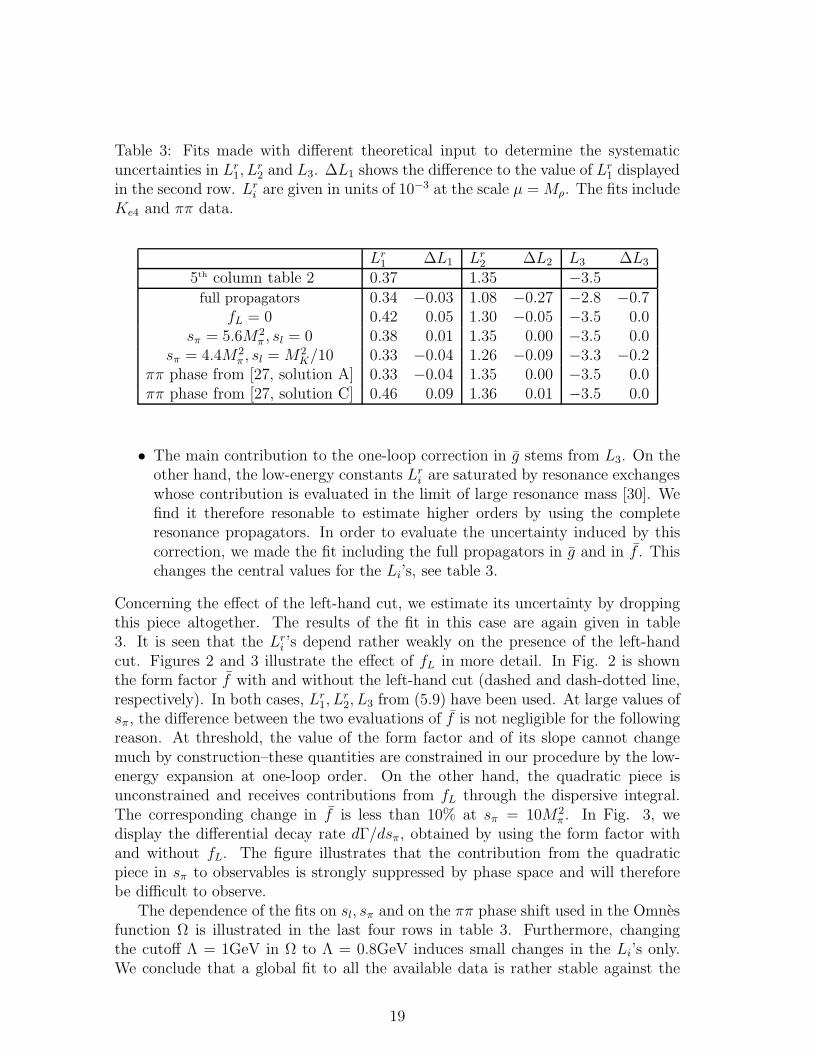
Table 3: Fits made with different theoretical input to determine the systematicuncertainties in Lr

1, Lr2 and L3. ∆L1 shows the difference to the value of Lr

1 displayedin the second row. Lr

i are given in units of 10−3 at the scale µ = Mρ. The fits includeKe4 and ππ data.

Lr1 ∆L1 Lr

2 ∆L2 L3 ∆L3

5th column table 2 0.37 1.35 −3.5full propagators 0.34 −0.03 1.08 −0.27 −2.8 −0.7

fL = 0 0.42 0.05 1.30 −0.05 −3.5 0.0sπ = 5.6M2

π , sl = 0 0.38 0.01 1.35 0.00 −3.5 0.0sπ = 4.4M2

π , sl = M2K/10 0.33 −0.04 1.26 −0.09 −3.3 −0.2

ππ phase from [27, solution A] 0.33 −0.04 1.35 0.00 −3.5 0.0ππ phase from [27, solution C] 0.46 0.09 1.36 0.01 −3.5 0.0

• The main contribution to the one-loop correction in g stems from L3. On theother hand, the low-energy constants Lr

i are saturated by resonance exchangeswhose contribution is evaluated in the limit of large resonance mass [30]. Wefind it therefore resonable to estimate higher orders by using the completeresonance propagators. In order to evaluate the uncertainty induced by thiscorrection, we made the fit including the full propagators in g and in f . Thischanges the central values for the Li’s, see table 3.

Concerning the effect of the left-hand cut, we estimate its uncertainty by droppingthis piece altogether. The results of the fit in this case are again given in table3. It is seen that the Lr

i ’s depend rather weakly on the presence of the left-handcut. Figures 2 and 3 illustrate the effect of fL in more detail. In Fig. 2 is shownthe form factor f with and without the left-hand cut (dashed and dash-dotted line,respectively). In both cases, Lr

1, Lr2, L3 from (5.9) have been used. At large values of

sπ, the difference between the two evaluations of f is not negligible for the followingreason. At threshold, the value of the form factor and of its slope cannot changemuch by construction–these quantities are constrained in our procedure by the low-energy expansion at one-loop order. On the other hand, the quadratic piece isunconstrained and receives contributions from fL through the dispersive integral.The corresponding change in f is less than 10% at sπ = 10M2

π . In Fig. 3, wedisplay the differential decay rate dΓ/dsπ, obtained by using the form factor withand without fL. The figure illustrates that the contribution from the quadraticpiece in sπ to observables is strongly suppressed by phase space and will thereforebe difficult to observe.

The dependence of the fits on sl, sπ and on the ππ phase shift used in the Omnesfunction Ω is illustrated in the last four rows in table 3. Furthermore, changingthe cutoff Λ = 1GeV in Ω to Λ = 0.8GeV induces small changes in the Li’s only.We conclude that a global fit to all the available data is rather stable against the

19

systematic uncertainties considered here.To finally give the best determinations of Lr

1, Lr2 and L3, we take the central

values from the global fit displayed in table 2, column 5. For the correspondingerrors, we take the ones generated by using the theoretical error bars for the higherorders in g, and find in this manner

103Lr1(Mρ) = 0.4± 0.3 ,

103Lr2(Mρ) = 1.35± 0.3 ,

103L3(Mρ) = −3.5± 1.1 .(5.9)

For SU(2)L × SU(2)R analyses it is useful to know the corresponding values for theconstants l1 and l2,

l1 = −1.7 ± 1.0 ,l2 = 6.1± 0.5 .

(5.10)

The value and uncertainties in these couplings play a decisive role in a plannedexperiment [31] to measure the lifetime of π+π− atoms, which will provide a com-pletely independent measurement of the ππ scattering lengths |a00 − a20|.

One motivation for the analysis in [8, 9] was to test the large NC predictionLr2 = 2Lr

1. The above result shows that a small non-zero value is preferred. To obtaina clean error analysis, we have repeated the fitting procedure using the variables

X1 = Lr2 − 2Lr

1 − L3 ,

Xr2 = Lr

2 ,

X3 = (Lr2 − 2Lr

1)/L3 .

We performed a fit to Ke4 and ππ data, including the theoretical error in G asdiscussed above, and found

X1 = (4.8± 0.8) · 10−3 ,

X3 = −0.17+0.12−0.22 . (5.11)

The result is that the large NC prediction works remarkably well.

5.3 Comparison with earlier work

It is of interest to compare the present procedure to determine the low-energy con-stants Lr

1, Lr2 and L3 with the method used in [9]. There are two main differences:

1. The definition of the slope λf and of the threshold value of the form factors fs, gchosen in [9] differs from the one used here. These quantities have of course aunique meaning in principle – on the other hand, one may wish to approximatea particular experimental situation. The procedure used in [9] was adapted toRef. [11], whereas a slight variation of the method proposed here may be usefulonce the sl-dependence of the form factors has experimentally been resolved.

20

2. Higher order corrections are estimated in [9] in a rather crude manner. In thepresent approach, the final-state interactions in the I = 0, S-wave amplitudeare instead taken into account, and higher order terms in g are estimated withresonance exchange.

The main effect of these differences can be described as follows. The differentslope and form factors used in [9] lead to slightly different central values for Lr

1, Lr2

and L3 at one-loop order, whereas the errors turn out to be very similar in bothcases. The higher order estimates in [9] lead to the same central values with largererror bars, whereas the unitarization performed in the present work leads to differentcentral values with slightly smaller error bars than before, see columns 2/3 and 4/5 intable 2. This effect can be easily understood by considering the simplified expression(4.11), which shows how the Omnes function affects the influence of the Li’s andhence their value in the fit.

5.4 Improvements

As we mentioned at the beginning of this section, there is room for improvement inthe above treatment, both on the theoretical and on the experimental side. Con-cerning the latter, one should determine in future experiments the form factors fsand g without additional assumptions [11] which are in contradiction with the chiralrepresentation. It remains to be seen whether this can be achieved by comparingthe data directly with a modified chiral representation. In the latter, the full S-and P - wave parts of F1 and F2 could be inserted, using the chiral representationsolely to describe the small background effects due to higher partial waves l ≥ 2.To be more precise, one would take for R and H the one-loop chiral representation,whereas for G one writes

G = g(sπ, sl)eiδp +∆G ,

∆G = GCHPT − 3

8π

∫

dΩ sin2 θπGCHPT , (5.12)

and similarly for F . The unknown amplitudes g(sπ, sl), fs(sπ, sl) and the phasesδp, δs would then be determined from the data. We have checked that, if the errorsin the form factors determined in this manner can be reduced by e.g. a factor 3 withrespect to the ones shown in (5.4), one could pin down particular combinations ofLr1, L

r2 and L3 to considerably better precision than was shown above. This is true

independently of an eventual improvement in the theoretical determination of thehigher order corrections in the form factor G – which is a theoretical challenge inany case.

6 Predictions

Having determined the constants Lr1, L

r2 and L3, there are several predictions which

we can make. Whereas the slope λg was assumed to coincide with the slope λf in

21

the final analysis of the data in Ref. [11], these two quantities may differ in thechiral representation. Furthermore, our amplitudes allow us to evaluate partial andtotal decay rates. In this section, we consider the slope λg and the total rates.

6.1 The slope λg

We consider the form factor g introduced in (5.6) and determine its slope λg

g(sπ, sl) = g(4M2π , sl)(1 + λg(sl)q

2 +O(q4)) (6.1)

from the one-loop expression for G. The result is λg(0) = 0.08. As the slope isa one-loop effect, higher order corrections may affect its value substantially. Forthis reason, we have evaluated λg also from the modified form factor obtained byusing the complete resonance propagators (and the corresponding Li’s), comparethe discussion above. The change is ∆λg = 0.025. We believe this to be a generouserror estimate and obtain in this manner

λg(0) = 0.08± 0.025 . (6.2)

The central value indeed agrees with the slope λf in (5.4).

6.2 Total rates

Once the leading partial waves f and g are known from e.g. K+ → π+π−e+νe decays,the chiral representation allows one to predict the remaining rates within rathersmall uncertainties. We illustrate the procedure for K+ → π0π0e+νe. Accordingto Eq. (2.18), the relevant amplitude is determined by F+, G−, R+ and H−. Thecontribution from H is kinematically strongly suppressed and completely negligiblein all total rates, whereas the contribution from R is negligible in the electron modes.Using the chiral representation of the amplitudes F+ and G−, we find that the rateis reproduced to about 1%, if one neglects G− altogether and uses only the leadingpartial wave in the remaining amplitude, F+

1 ≃ −Xf . From the measured [11] formfactor f = 5.59(1 + 0.08q2) we then find ΓK+→π0π0e+νe = 1625sec−1. Finally, weestimate the error from

∆Γ =

[Γ(fs(0) + ∆fs, λf)− Γ(fs(0), λf)]2+

[Γ(fs(0), λf +∆λf )− Γ(fs(0), λf)]21/2

= 90sec−1 ,

(6.3)

where ∆fs = 0.14,∆λf = 0.02. The final result for the rate is shown in the row”final prediction” in table 5, where we have also listed the tree and the one-loopresult, together with the experimental data. The evaluation of the remaining ratesis done in a similar manner – see table 4 for the simplifications used and table 5 forthe corresponding predictions.

22

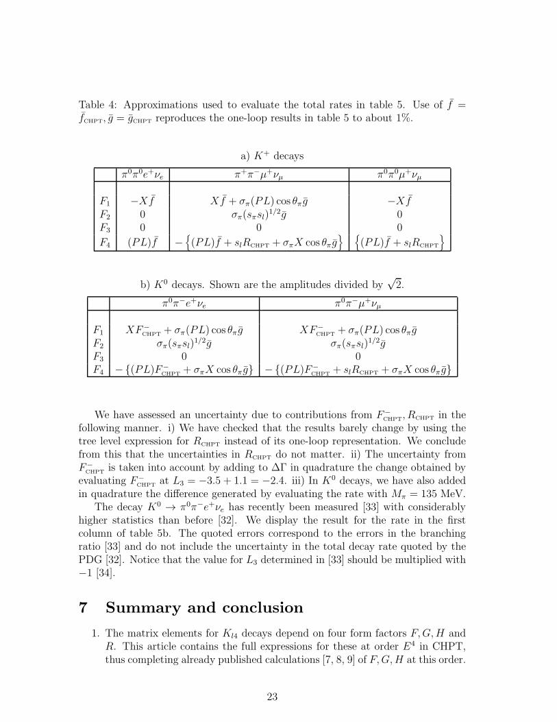
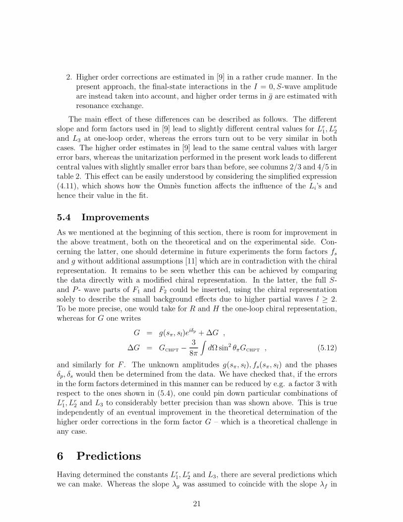
Table 4: Approximations used to evaluate the total rates in table 5. Use of f =fCHPT, g = gCHPT reproduces the one-loop results in table 5 to about 1%.

a) K+ decays

π0π0e+νe π+π−µ+νµ π0π0µ+νµ

F1 −Xf Xf + σπ(PL) cos θπ g −XfF2 0 σπ(sπsl)

1/2g 0F3 0 0 0

F4 (PL)f −

(PL)f + slRCHPT + σπX cos θπg

(PL)f + slRCHPT

b) K0 decays. Shown are the amplitudes divided by√2.

π0π−e+νe π0π−µ+νµ

F1 XF−

CHPT+ σπ(PL) cos θπ g XF−

CHPT+ σπ(PL) cos θπg

F2 σπ(sπsl)1/2g σπ(sπsl)

1/2gF3 0 0F4 −(PL)F−

CHPT+ σπX cos θπ g −(PL)F−

CHPT+ slRCHPT + σπX cos θπ g

We have assessed an uncertainty due to contributions from F−

CHPT, RCHPT in the

following manner. i) We have checked that the results barely change by using thetree level expression for RCHPT instead of its one-loop representation. We concludefrom this that the uncertainties in RCHPT do not matter. ii) The uncertainty fromF−

CHPTis taken into account by adding to ∆Γ in quadrature the change obtained by

evaluating F−

CHPTat L3 = −3.5 + 1.1 = −2.4. iii) In K0 decays, we have also added

in quadrature the difference generated by evaluating the rate with Mπ = 135 MeV.The decay K0 → π0π−e+νe has recently been measured [33] with considerably

higher statistics than before [32]. We display the result for the rate in the firstcolumn of table 5b. The quoted errors correspond to the errors in the branchingratio [33] and do not include the uncertainty in the total decay rate quoted by thePDG [32]. Notice that the value for L3 determined in [33] should be multiplied with−1 [34].

7 Summary and conclusion

1. The matrix elements for Kl4 decays depend on four form factors F,G,H andR. This article contains the full expressions for these at order E4 in CHPT,thus completing already published calculations [7, 8, 9] of F,G,H at this order.

23

Table 5: Total decay rates in sec−1. To evaluate the rates at one-loop accuracy,we have used Lr

1, Lr2 and L3 from (5.9). The remaining low-energy constants are

from table 1. The final predictions are evaluated with the amplitudes shown intable 4, using f = 5.59(1 + 0.08q2), g = 4.77(1 + 0.08q2). For the evaluation of theuncertainties in the rates see text.

a) K+ decays

π+π−e+νe π0π0e+νe π+π−µ+νµ π0π0µ+νµtree 1297 683 155 102

one-loop 2447 1301 288 189final input 1625 333 225

prediction ±90 ±15 ±11experiment 3160 1700 1130

[32] ±140 ±320 ±730

b) K0 decays

π0π−e+νe π0π−µ+νµtree 561 55

one-loop 953 94final 917 88

prediction ±170 ±22experiment 998

[33] ±39± 43

2. We have estimated higher order terms in the S-wave amplitude of the formfactor F by use of a dispersive representation, determining the subtractionconstants in the standard manner [12] from CHPT. This procedure puts earlierattempts [9] to estimate these corrections on a more firm basis.

3. Using the improved S-wave amplitude, we have determined Lr1, L

r2 and L3 from

K+ → π+π−e+νe decays and ππ threshold data. Unitarizing the amplitudeaffects the related SU(2) × SU(2) constant l1 in a significant manner. Asa result of this, the D-wave scattering lengths are in better agreement withthe values given by Petersen [25] than was the case before [9]. All in all, aremarkably good agreement with Ke4 and ππ data is obtained.

4. Kl4 decays may be used to test the large-NC prediction Lr2 = 2Lr

1 [8, 9]. Usingthe improved representation of the amplitudes, we have confirmed the earlier[9] finding: The large-NC rule works at the one standard deviation level forthis combination of the constants.

24

5. The above determination of Lr1, L

r2 and L3 will presumably be even more reli-

able, once high statistics data from kaon facilities like DAΦNE [20] will becomeavailable.

6. We also predict the slope λg of the form factor G and total decay rates, seeEq. (6.2) and table 5.

7. We have made some effort to find out whether any of the Kl4 decays couldserve to determine some of the other low-energy constants which occur in theamplitude. We believe that it will be very difficult to pin down any of these(in particular Lr

4) to better precision than already known, because the higherorder corrections tend to wash out their effect.

8. Finally, we would like to recall that the determination of the low-energy con-stants from Kl4 decays or the prediction of the total rates is not the only issue:these decays are in addition the only known source for a precise determina-tion of the isoscalar ππ S-wave phase shift near threshold. The possibilitiesto determine those in future high statistics experiments are presently underinvestigation [35].

Acknowledgements

It is a pleasure to thank Gerhard Ecker, Marc Knecht and Jan Stern for enjoy-able discussions and Greg Makoff for communications concerning the experimentdescribed in [33].

25

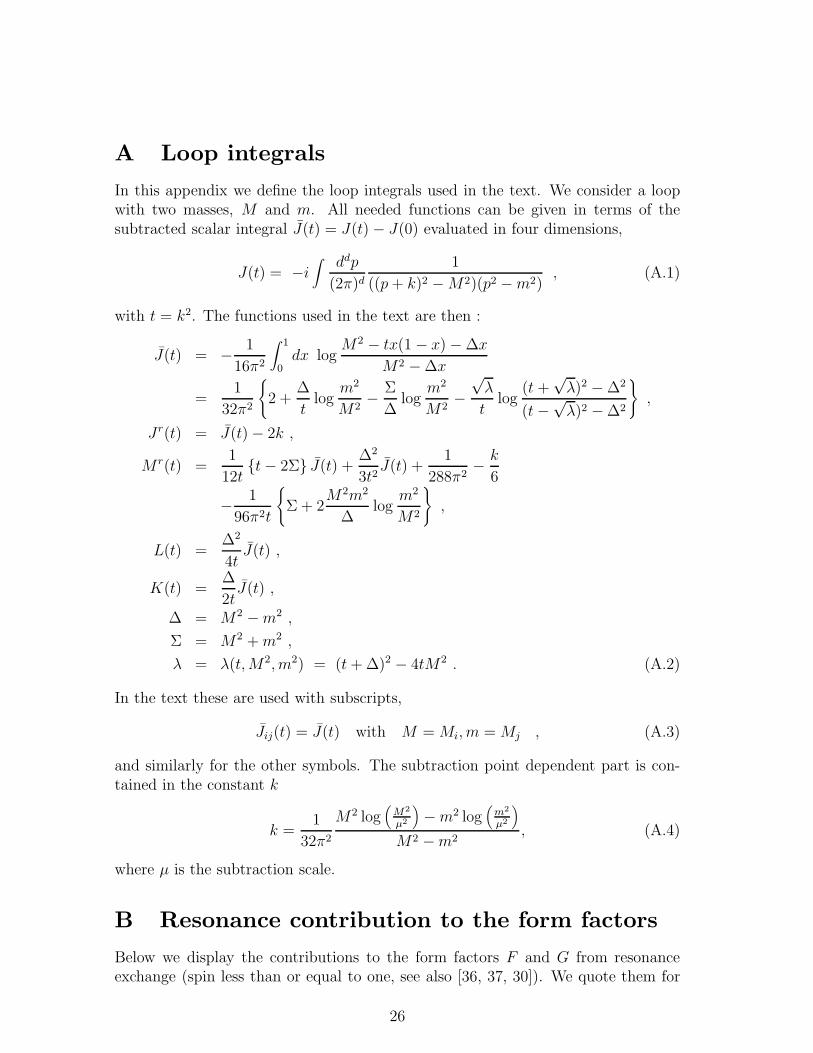
A Loop integrals

In this appendix we define the loop integrals used in the text. We consider a loopwith two masses, M and m. All needed functions can be given in terms of thesubtracted scalar integral J(t) = J(t)− J(0) evaluated in four dimensions,

J(t) = −i∫ ddp

(2π)d1

((p+ k)2 −M2)(p2 −m2), (A.1)

with t = k2. The functions used in the text are then :

J(t) = − 1

16π2

∫ 1

0dx log

M2 − tx(1 − x)−∆x

M2 −∆x

=1

32π2

2 +∆

tlog

m2

M2− Σ

∆log

m2

M2−

√λ

tlog

(t +√λ)2 −∆2

(t−√λ)2 −∆2

,

Jr(t) = J(t)− 2k ,

M r(t) =1

12tt− 2Σ J(t) + ∆2

3t2J(t) +

1

288π2− k

6

− 1

96π2t

Σ+ 2M2m2

∆log

m2

M2

,

L(t) =∆2

4tJ(t) ,

K(t) =∆

2tJ(t) ,

∆ = M2 −m2 ,

Σ = M2 +m2 ,

λ = λ(t,M2, m2) = (t+∆)2 − 4tM2 . (A.2)

In the text these are used with subscripts,

Jij(t) = J(t) with M = Mi, m = Mj , (A.3)

and similarly for the other symbols. The subtraction point dependent part is con-tained in the constant k

k =1

32π2

M2 log(

M2

µ2

)

−m2 log(

m2

µ2

)

M2 −m2, (A.4)

where µ is the subtraction scale.

B Resonance contribution to the form factors

Below we display the contributions to the form factors F and G from resonanceexchange (spin less than or equal to one, see also [36, 37, 30]). We quote them for

26

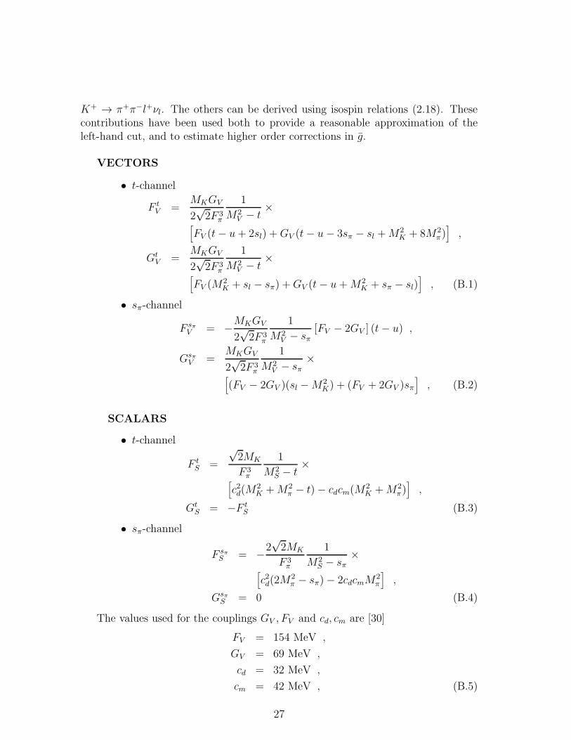
K+ → π+π−l+νl. The others can be derived using isospin relations (2.18). Thesecontributions have been used both to provide a reasonable approximation of theleft-hand cut, and to estimate higher order corrections in g.

VECTORS

• t-channel

F tV =

MKGV

2√2F 3

π

1

M2V − t

×[

FV (t− u+ 2sl) +GV (t− u− 3sπ − sl +M2K + 8M2

π)]

,

GtV =

MKGV

2√2F 3

π

1

M2V − t

×[

FV (M2K + sl − sπ) +GV (t− u+M2

K + sπ − sl)]

, (B.1)

• sπ-channel

F sπV = −MKGV

2√2F 3

π

1

M2V − sπ

[FV − 2GV ] (t− u) ,

GsπV =

MKGV

2√2F 3

π

1

M2V − sπ

×[

(FV − 2GV )(sl −M2K) + (FV + 2GV )sπ

]

, (B.2)

SCALARS

• t-channel

F tS =

√2MK

F 3π

1

M2S − t

×[

c2d(M2K +M2

π − t)− cdcm(M2K +M2

π)]

,

GtS = −F t

S (B.3)

• sπ-channel

F sπS = −2

√2MK

F 3π

1

M2S − sπ

×[

c2d(2M2π − sπ)− 2cdcmM

2π

]

,

GsπS = 0 (B.4)

The values used for the couplings GV , FV and cd, cm are [30]

FV = 154 MeV ,

GV = 69 MeV ,

cd = 32 MeV ,

cm = 42 MeV , (B.5)

27

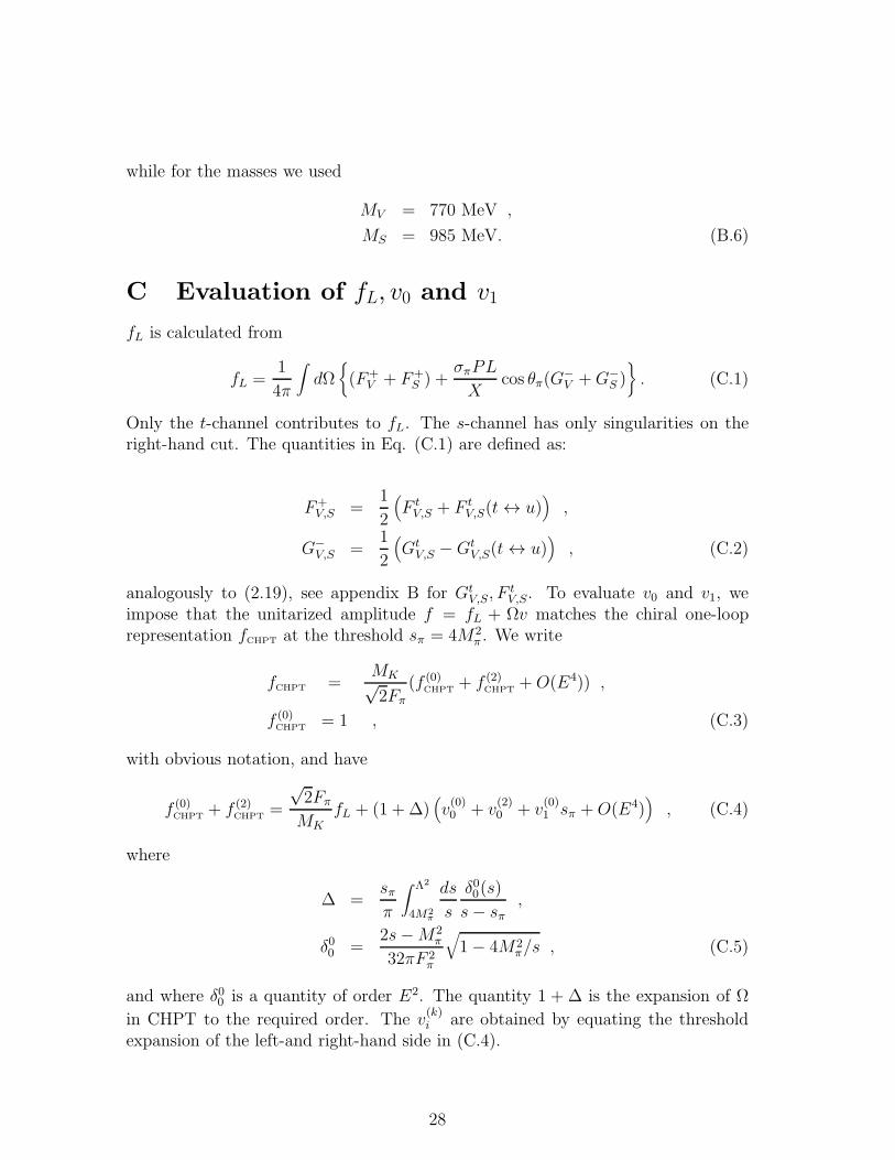
while for the masses we used

MV = 770 MeV ,

MS = 985 MeV. (B.6)

C Evaluation of fL, v0 and v1

fL is calculated from

fL =1

4π

∫

dΩ

(F+V + F+

S ) +σπPL

Xcos θπ(G

−

V +G−

S )

. (C.1)

Only the t-channel contributes to fL. The s-channel has only singularities on theright-hand cut. The quantities in Eq. (C.1) are defined as:

F+V,S =

1

2

(

F tV,S + F t

V,S(t ↔ u))

,

G−

V,S =1

2

(

GtV,S −Gt

V,S(t ↔ u))

, (C.2)

analogously to (2.19), see appendix B for GtV,S, F

tV,S. To evaluate v0 and v1, we

impose that the unitarized amplitude f = fL + Ωv matches the chiral one-looprepresentation fCHPT at the threshold sπ = 4M2

π . We write

fCHPT =MK√2Fπ

(f (0)CHPT

+ f (2)CHPT

+O(E4)) ,

f (0)CHPT

= 1 , (C.3)

with obvious notation, and have

f (0)CHPT

+ f (2)CHPT

=

√2Fπ

MKfL + (1 + ∆)

(

v(0)0 + v

(2)0 + v

(0)1 sπ +O(E4)

)

, (C.4)

where

∆ =sππ

∫ Λ2

4M2π

ds

s

δ00(s)

s− sπ,

δ00 =2s−M2

π

32πF 2π

√

1− 4M2π/s , (C.5)

and where δ00 is a quantity of order E2. The quantity 1 + ∆ is the expansion of Ω

in CHPT to the required order. The v(k)i are obtained by equating the threshold

expansion of the left-and right-hand side in (C.4).

28

References

[1] S. Weinberg, Physica 96A (1979) 327.

[2] J. Gasser and H. Leutwyler, Ann. Phys. (N.Y.) 158 (1984) 142.

[3] J. Gasser and H. Leutwyler, Nucl. Phys. B250 (1985) 465.

[4] H. Leutwyler, Bern University preprint BUTP-93/24 (hep-ph/9311274).

[5] For recent reviews on CHPT see e.g.H. Leutwyler, in: Proc. XXVI Int. Conf. on High Energy Physics, Dallas, 1992,edited by J.R. Sanford, AIP Conf. Proc. No. 272 (AIP, New York, 1993) p. 185;U.G. Meißner, Rep. Prog. Phys. 56 (1993) 903;A. Pich, Lectures given at the V Mexican School of Particles and Fields, Guana-juato, Mexico, December 1992, preprint CERN-Th.6978/93 (hep-ph/9308351);G. Ecker, Lectures given at the 6th Indian–Summer School on IntermediateEnergy Physics Interaction in Hadronic Systems Prague, August 25 - 31, 1993,to appear in the Proceedings (Czech. J. Phys.), preprint UWThPh -1993-31(hep-ph/9309268).

[6] S. Weinberg, Phys. Rev. Lett. 17 (1966) 336; 18 (1967) 1178 E.

[7] J. Wess and B. Zumino, Phys. Lett. 37B (1971) 95.

[8] J. Bijnens, Nucl. Phys. B337 (1990) 635.

[9] C. Riggenbach, J. Gasser, J.F. Donoghue and B.R. Holstein, Phys. Rev. D43(1991) 127.

[10] Ll. Ametller, J. Bijnens, A. Bramon and F. Cornet, Phys. Lett. B303 (1993)140.

[11] L. Rosselet et al., Phys. Rev. D15 (1977) 574.

[12] J. Donoghue, J. Gasser and H. Leutwyler, Nucl. Phys. B343 (1990) 341.

[13] N. Cabibbo and A. Maksymowicz, Phys. Rev. B137 (1965) B438; Phys. Rev.168 (1968) 1926 E.

[14] A. Pais and S.B. Treiman, Phys. Rev. 168 (1968) 1858.

[15] F.A. Berends, A. Donnachie and G.C. Oades, Phys. Lett. 26B (1967) 109; Phys.Rev. 171 (1968) 1457.

[16] L.-M. Chounet, J.-M. Gaillard and M.K. Gaillard, Phys. Rep. C4 (1972) 199.

[17] E.P. Shabalin, Yad. Fiz. 49 (1989) 588 [Sov. J. Nucl. Phys. 49 (1989) 365]; ibid.51 (1990) 464 [Sov. J. Nucl. Phys. 51 (1990) 296].

29

[18] M. Knecht, H. Sazdjian, J. Stern and N.H. Fuchs, Phys. Lett. B313 (1993) 229.

[19] J. Bijnens, G. Ecker and J. Gasser, in [20], p.115.

[20] The DAΦNE Physics Handbook, edited by L. Maiani, G. Pancheri and N. Paver(INFN, Frascati, 1992).

[21] J. Wess and B. Zumino, Phys. Lett. 37B (1971) 95;E. Witten, Nucl. Phys. B223 (1983) 422;N.K. Pak and P. Rossi, Nucl. Phys. B250 (1985) 279.

[22] T.N. Truong, Phys. Rev. Lett. 61 (1988) 2526.

[23] T.N. Truong, Phys. Lett. 99B (1981) 154.

[24] A.D. Martin and T.D. Spearman, Elementary particle theory (North-Holland,Amsterdam, 1970) p.1.

[25] M.M. Nagels et al., Nucl. Phys. 147 (1979) 189.

[26] MINUIT Reference Manual, Application Software Group, Computing and Net-work Division, CERN.

[27] A. Schenk, Nucl. Phys. B363 (1991) 97.

[28] T.N. Pham and T.N. Truong, Phys. Rev. D31 (1985) 3027.

[29] J. Stern, H. Sazdjian and N.H. Fuchs, Phys. Rev. 47 (1993) 3814.

[30] G.Ecker, J.Gasser, A.Pich and E.de Rafael, Nucl. Phys. B321 (1989) 311.

[31] G. Czapek et al., Letter of intent: Lifetime measurements of π+π− atoms totest low-energy QCD predictions, preprint CERN/SPSLC 02-44.

[32] Particle Data Group (K. Hikasa et al.), Phys. Rev. D45 (1992) S1.

[33] G.Makoff et al., Phys. Rev. Lett. 70 (1993) 1591.

[34] G. Makoff, private communication.

[35] The DAΦNE working group; H. Kaspar, private communication.

[36] P. Ko, Phys. Rev. D46 (1992) 3813; D47 (1993) 1250.

[37] M. Finkemeier, Phys. Rev. D47 (1993) 1933.

30

Figure captions

Fig. 1 Kinematic variables for Kl4 decays. The angle θπ is defined in Σ2π, θl in Σlν

and φ in ΣK .

Fig. 2 The partial wave amplitude f(sπ, sl = 0). The dashed line shows f , evaluatedaccording to Eqs. (4.10,C.1), with Lr

1, Lr2 and L3 from (5.9). The dash-dotted

line is evaluated with fL = 0 according to (4.11), using the same Li’s, whereasthe solid line displays fs = 5.59(1 + 0.08q2).

Fig. 3 Differential rate dΓ/dsπ for K+ → π+π−e+νe decays in arbitrary units. Theevaluation is done with F−

1 = F2 = F3 = F−

4 = 0, and F+1 = Xf(sπ, sl =

0), F+4 = −PL/XF+

1 . The input for the dashed (dash-dotted) line is the sameas for the dashed (dash-dotted) line in Fig. 2.

31

This figure "fig1-1.png" is available in "png" format from:

http://arxiv.org/ps/hep-ph/9403390v1

This figure "fig1-2.png" is available in "png" format from:

http://arxiv.org/ps/hep-ph/9403390v1