by hui bian office for faculty excellence - piratepanelcore.ecu.edu/ofe/statisticsresearch/logistic...
TRANSCRIPT
By Hui Bian
Office for Faculty Excellence
1

Contact information
Email: [email protected]
Phone: 328-5428
Location: 2307 Old Cafeteria Complex
(east campus)
Website: http://core.ecu.edu/ofe/StatisticsResearch/
2
What is logistic regression
According to IBM SPSS Manual
It is used to predict the presence or absence of a
characteristic or outcome based on values of a set of
predictor variables. It is similar to a linear regression
model, but suited to models where the dependent
variable is dichotomous.
The ultimate goal of logistic regression
to determine the probability of a case belonging to the
1 category of dependent variable or the probability of
event occurring (event occurring is always coded as
1) for a given set of predictors.
3

Variables in logistic regression
Dependent variable: one dichotomous/binary
variable
Yes/No: drug users vs. non-drug users
Membership: intervention vs. control
Characteristics: males vs. females
Independent variables: interval or dummy or
categorical variables (indicator coded).
Indicator coded: SPSS will automatically recode
categorical variable for us.
4

Assumptions
Homogeneity of variance and normality
of errors are NOT assumed, but it
requires:
Absence of multicollinearity
No specification errors: all relevant
predictors are included and irrelevant
predictors are excluded.
Larger sample size than using linear
regression
5
Logistic regression equation
Equation: Logit function
ln(p/1-p) =a + b1x1+b2x2+…+bnxn
Logit (p) = a + b1x1+b2x2+…+bnxn
6
p: probability of a case belonging to category 1
p/1-p: odds
a: constant
n: number of predictors
b1-bn: regression coefficients

Logistic regression equation
Non-linear relationship between predictors and
binary outcome.
The regression coefficients are estimated using
maximum likelihood.
7

Logistic regression curve
8
The Y-axis is P
(probability),
which indicates
the proportion of
1 at any given
value of X.

Coding of variables
Recommendation for dependent
variable
Use 1 as the event occurring (the focus of
the study)
Use 0 as absence of event (the reference
category)
SPSS automatically recodes the lower
number of the category to 0 and higher
number to 1.
9
Coding of variables
Recommendation for independent
variables
Coded as 1 for the category that is the focus
of the study
Coded as 0 for the category of reference
10

Coding of variables
Cases coded as 1 referred to as the
response group, comparison group, or
target group.
Cases coded as 0 referred to as the
reference group, base group, or control
group.
11

Terms
Probability: likelihood of an event
occurring Drug use status is DV and gender is IV.
The probability of a student using drug is 205/413=.496
We want to know whether this proportion is the same for
both males and females.
12
Drug users Non-users Total
Male 120 102 222
Female 85 106 191
Total 205 208 413

Terms
Odds: the probability of belonging to one group or
event occurring divided by the probability of not
belonging to that group or event not occurring.
The odds of a male using drug is 120/102=1.18,
The odds of a female using drug is 85/106= .80
For males, it means that a male is 1.18 times as
likely to use drug as not to use.
13
Drug users Non-users Total
Male 120 102 222
Female 85 106 191
Total 205 208 413

Terms
Odds ratio: an important estimate in logistic
regression and used to answer our research
question.
For the table below, the research question is
whether there is a gender difference in using
drugs or whether the probability of drug use is
the same for males and females.
14
Drug users (1) Non-users (0) Total
Male (1) 120 102 222
Female (0) 85 106 191
Total 205 208 413

Terms
Odds ratio
A ratio of the odds for each group.
Always odd for the response group (males)
divided by odd for the referent group
(females).
Odds ratio is 1.18/.80= 1.48
15
Drug users (1) Non-users (0) Total
Male (1) 120 102 222
Female (0) 85 106 191
Total 205 208 413

Terms
Odds ratio
Males in this example were 1.48 times more
likely than females to use drugs.
An odds ratio > 1 indicates that the likelihood of
an event occurring is more likely for the
response category than the referent category of
an independent variable.
An odds ratio < 1 indicates that the likelihood of
an event occurring is less likely for the response
category than the referent category of an
independent variable.
16
Terms
Adjusted odds ratio
When multiple independent variables in the
model
It indicates the contribution of a particular
predictor when other predictors are
controlled.
17

Terms
Ordinary least squares (OLS)
A method used for a linear regression model.
It minimizes the sum of squared vertical distances between the
observed responses in the dataset and the responses predicted
by the linear model.
Maximum likelihood estimation (MLE)
It is more appropriate for logistic regression model.
It maximizes the log likelihood.
The log likelihood indicates how likely the observed grouping can
be predicted from observed values of predictors.
18

Logistic regression using SPSS
Example of logistic regression analysis
Research question is whether a gender, self-control, and self-efficacy predict drug use status.
Three predictors
○ Gender (a01: 1 = males, 0 = females)
○ Self-control (continuous variable)
○ Self-efficacy (a80r: 1 =somewhat-not sure, 0 = very sure)
One dependent variable
○ Drug use status (1 = drug users, 0 =non-users)
19

Logistic regression
Null hypothesis
There is an equal chance of drug use or not
use for a given set of predictors or
The model coefficients are 0 (0 means
there is no change due to the predictor
variable).
20

Logistic regression using SPSS
Analyze > Regression > Binary Logistic
Enter Drug_use to Dependent
Enter a01, self-control, and a80r to
Covariates
21
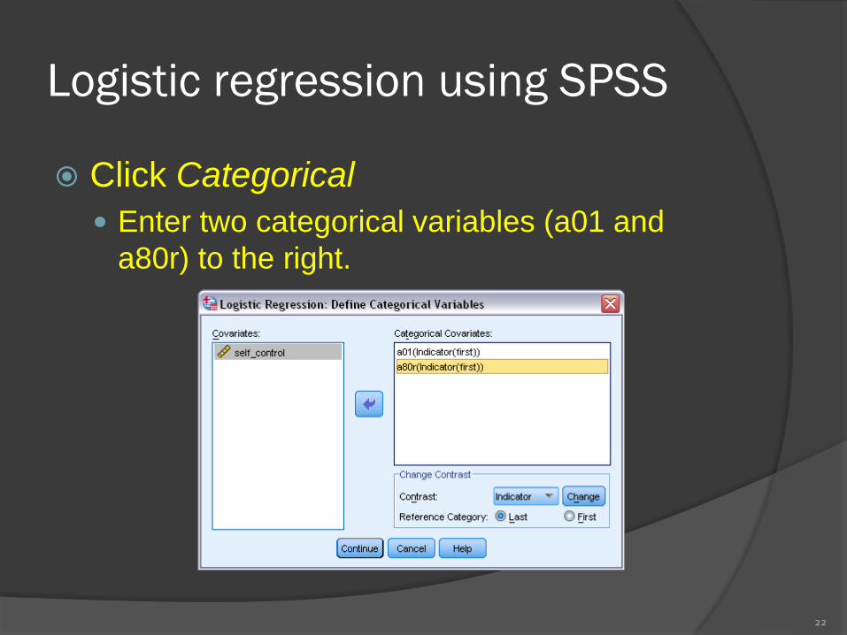
Logistic regression using SPSS
Click Categorical
Enter two categorical variables (a01 and
a80r) to the right.
22

Logistic regression using SPSS
Categorical
The default contrast is Indicator and
reference category is Last.
23
Logistic regression using SPSS
Categorical: contrast methods Indicator. Contrasts indicate the presence or absence of
category membership. The reference category is represented
in the contrast matrix as a row of zeros.
Simple. Each category of the predictor variable (except the
reference category) is compared to the reference category.
Difference. Each category of the predictor variable except the
first category is compared to the average effect of previous
categories. Also known as reverse Helmert contrasts.
Helmert. Each category of the predictor variable except the
last category is compared to the average effect of subsequent
categories.
24

Logistic regression using SPSS
Categorical: contrast
Repeated. Each category of the predictor
variable except the first category is compared to
the category that precedes it.
Polynomial. Orthogonal polynomial contrasts.
Categories are assumed to be equally spaced.
Polynomial contrasts are available for numeric
variables only.
Deviation. Each category of the predictor
variable except the reference category is
compared to the overall effect.
25

Logistic regression using SPSS
Categorical
For a01 and a80r, we want category 0 as a
reference category.
Check First
Then click Change
26

Logistic regression using SPSS
Save
27
For each case, if the
predicted probability
is greater than 0.5,
then this respondent
would be predicted to
use drug (coded as
1).
If the predicted
probability is less than
0.5, this respondent
would be predicted to
not use drug (coded
as 0).

Logistic regression using SPSS
Options
28

SPSS output
Coding
29
Our coding is the same as the Parameter coding

SPSS output
30
Constant-only-model:
Block 0 (beginning block/step
0) means only constant is in
the model and our predictors
are not in the equation yet.

SPSS output
Block 1
31
Full model:
Block1 (step1) indicates that
our predictors are entered the
model simultaneously. The
method used is Enter.
Validity of the model:
The null hypothesis is
rejected (p < .05).
-2Log likelihood ratio
test: tests whether a set
of IVs improves
prediction of DV better
than chance.
Pseudo R square:
Nagelkerke R2 is preferred.
The model accounts for
almost 10% of variance of
DV.
This test assesses
whether the predicted
probabilities match the
observed probabilities. P
> .05 means a set of IVs
will accurately predict the
actual probabilities.
Model fit
statistics
SPSS output
Model fit: Goodness-of-fit statistics help you to
determine whether the model adequately
describes the data.
-2 log likelihood test (-2LL)
Omnibus test of model coefficients: Chi-square,
it is based on the null hypothesis that all the
coefficients are zero.
Model summary
Pseudo R2
Homer and Lemeshow Test
32

SPSS output
The overall predictive accuracy is 62.7%.
33
In block 0, the probability of a correct prediction is
50.4%. In block 1, the overall predictive accuracy is
62.7%.
Block 1

SPSS output
Classification table
64.9% is also known as the sensitivity of
prediction.
60.6% is also known as the specificity of
prediction.
34

SPSS output
Variables in the equation
35
1. Wald test
It tests the effect of individual predictor while controlling other predictors.
2. Exp(B)
It is an odds ratio. For gender, males are 1.60 times more likely to use
drugs than females. For self-control, the probability of drug use is
contingent on self-control level. Higher score of self-control, less likely to
use drugs. For a80r, low self-efficacy group is 1.53 times more likely to
use drugs than high self-efficacy group.
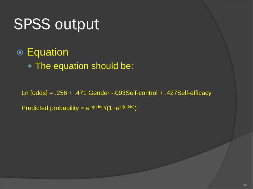
SPSS output
Equation
The equation should be:
36
Ln [odds] = .256 + .471 Gender -.093Self-control + .427Self-efficacy
Predicted probability = eln(odds)/(1+eln(odds))
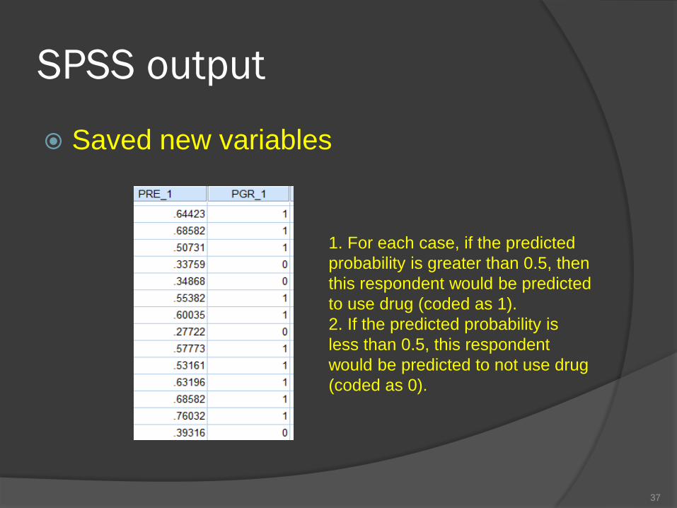
SPSS output
Saved new variables
37
1. For each case, if the predicted
probability is greater than 0.5, then
this respondent would be predicted
to use drug (coded as 1).
2. If the predicted probability is
less than 0.5, this respondent
would be predicted to not use drug
(coded as 0).

Results
38
The logistic regression was performed to test effects of
self-control, self-efficacy, and gender on drug use.
Results indicated that the three-predictor model provided
a statistically significant improvement over the constant-
only-model, χ2(3, N= 413) = 31.36, p = .00. The
Nagelkerke R2 indicated that the model accounted for
9.8% of the total variance. The correct prediction rate
was about 63.7% . The Wald tests showed that all three
predictors significantly predicted drug use status.

Logistic regression using SPSS
Independent variables are categorical
variables with more than 2 categories.
Example: add a93a (My friends think that it's
okay for me to drinks too much alcohol) into
the model as an independent variable.
Rerun previous logistic regression
Use Indicator method and first level as a
reference.
39
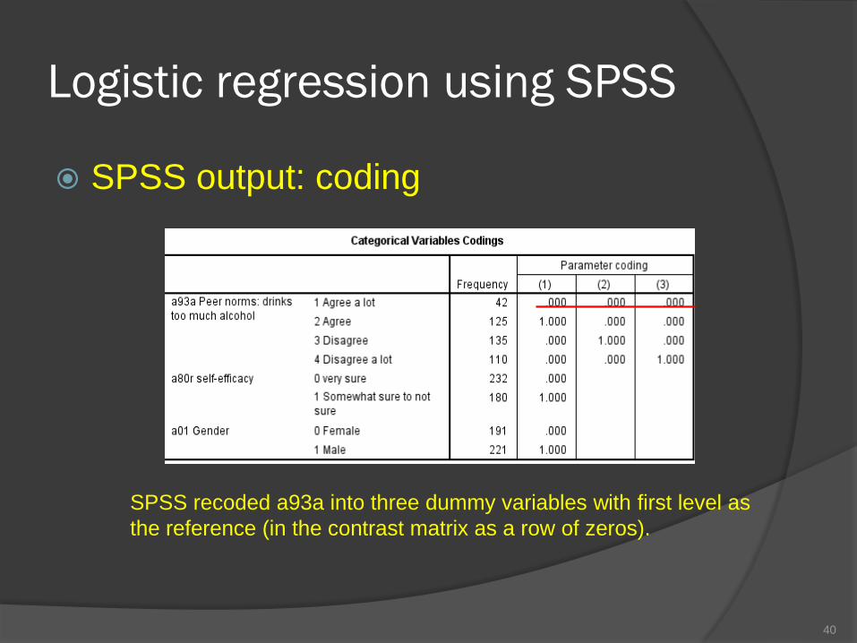
Logistic regression using SPSS
SPSS output: coding
40
SPSS recoded a93a into three dummy variables with first level as
the reference (in the contrast matrix as a row of zeros).

Logistic regression using SPSS
SPSS output: Variables in the equation
41

Comparing logistic models
Purpose of comparing logistic models
Whether adding more variables in the model will
provide an improvement in predictive power.
Example: we want to know whether there is a
significant interaction of self-efficacy and self-control
on probability of drug use.
Add interaction term (self-efficacy*self-control) to
the model
We are going to have three models: constant-only-
model, model with three predictors and constant,
and model with interaction term, three predictors,
and constant.
42

Comparing logistic models
Enter a01, a80r, and self-control to
Block1, then click Next.
43

Comparing logistic models
Block 2
44
Highlight a80r and
hold Control to select
self-control. Then
click a*b>, enter
a80r*self-control to
Block 2.

SPSS output
The results for Block 0 and Block 1 are
the same as those from the previous
study.
45
1. The Block 2 is not significant. It
means the interaction term is not
significant. Model means with
everything in the equation, the
whole model is significant.
2. The difference of -2Log Likelihood
between block 2 and 1 is 541.153-
537.486 = 3.68, this is a Chi-
square statistic with df = 1, p < .05
(check Chi-square table, Chi-
square = 3.84 as p =.05, df = 1)

SPSS output
46
The Chi-square change from Block1 to Block 2 is 35.032-31.364=3.668, which
is the Chi-square for interaction term. The R2 change indicates that 1% of
variance is explained by interaction term. The improvement of prediction is not
significant ( p = .055).

SPSS output
47
The Wald test also shows that there is no significant interaction effect
of self-efficacy and self-control on DV.
Equation of model: ln(odds) = .021 + .476 Gender -.063Self-control +
1.03 Self-efficacy -.079Self-efficacy * Self-control

Graphs for interaction effect
48

Graphs for interaction effect
49
Self-Efficacy:
1 = Somewhat
sure-not sure
Self-efficacy:
0 = Very sure

Multinomial logistic regression
Used to classify subjects based on
values of a set of predictor variables.
This type of regression is similar to
logistic regression, but it is more general
because the dependent variable is not
restricted to two categories.
50

Multinomial logistic regression
Variables
The dependent variable should be
categorical.
Independent variables can be factors or
covariates. In general, factors should be
categorical variables and covariates should
be continuous variables.
51

Multinomial logistic regression using SPSS
Example (from SPSS samples)
Regression to determine marketing profiles for
each breakfast option.
Dependent variable: Choice of breakfast: 1 =
Breakfast bar; 2 = Oatmeal; 3 = Cereal
Independent variables: age, gender, lifestyle (they
are all categorical variables)
52

Multinomial logistic regression using SPSS
Go to Analyze > Regression >
Multinomial Logistic
53

Multinomial logistic regression using SPSS
Click Reference Category
54
We can use any category of
dependent variable as the
reference.

Multinomial logistic regression using SPSS
55
Click Model
The default model is
Main effects. We can
custom our model
and request main
effects and
interaction effects.

Multinomial logistic regression using SPSS
Click Statistics
56
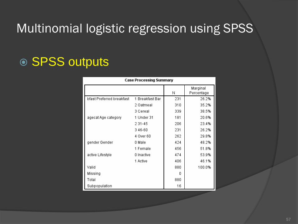
Multinomial logistic regression using SPSS
SPSS outputs
57

Multinomial logistic regression using SPSS
SPSS Output
58
Cells with zero frequencies can be a useful indicator for
potential problems. Since there are few (only 4.2%) of
these empty cells, you can probably safely use the results
of the goodness-of-fit tests.

Multinomial logistic regression using SPSS
SPSS Outputs
59
1. The likelihood ratio tests check
the difference between null
model and final model.
2. The Chi-Square in the first
table is the change of -2 Log
Likelihood from intercept-only-
model to the final model.
3. The results show that the final
model is outperforming the null.
3. Results of Goodness-of-Fit
show that the model adequately
fits the data.

Multinomial logistic regression using SPSS
SPSS Output
60
The likelihood ratio tests check
the contribution of each effect to
the model.
Age and Active make significant
contributions to the model.
Multinomial logistic regression using SPSS
SPSS Output
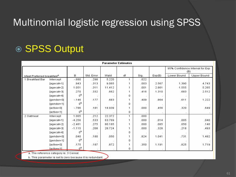
61

Multinomial logistic regression using SPSS
SPSS Output: Parameter estimates
table summarizes the effect of each
predictor.
Parameters with significant negative
coefficients decrease the likelihood of that
response category with respect to the
reference category.
Parameters with positive coefficients
increase the likelihood of that response
category.
62

Multinomial logistic regression using SPSS
SPSS Output
63
Cells on the diagonal are correct predictions and cells
off the diagonal are incorrect predictions.
Overall, 56.4% of the cases are classified correctly.

References
Agresti, A. & Finlay, B. (1997). Statistical methods for the social sciences (3rd ed.). Upper Saddle River, NJ: Prentice Hall, Inc.
Meyers, L. S., Gamst, G., & Guarino, A. J. (2006). Applied multivariate research: design and interpretation. Thousand Oaks, CA: Sage Publications, Inc.
Stevens, J. P. (2002). Applied multivariate statistics for the social sciences (4th ed.). Mahwah, NJ: Lawrence Erlbaum Associates, Inc.
64

65