by john philip morton b.a. b.a.i. (hons) this thesis …...- i - the dynamic measurement of...
TRANSCRIPT

- I -
THE DYNAMIC MEASUREMENT OF UNDRAINED SHEAR
STRENGTH USING AN INSTRUMENTED FREE FALLING
SPHERE
By
John Philip Morton
B.A. B.A.I. (Hons)
This thesis is submitted for the
Degree of Doctor of Philosophy
School of Civil, Environmental and Mining Engineering
2015

- II -
- III -
ABSTRACT
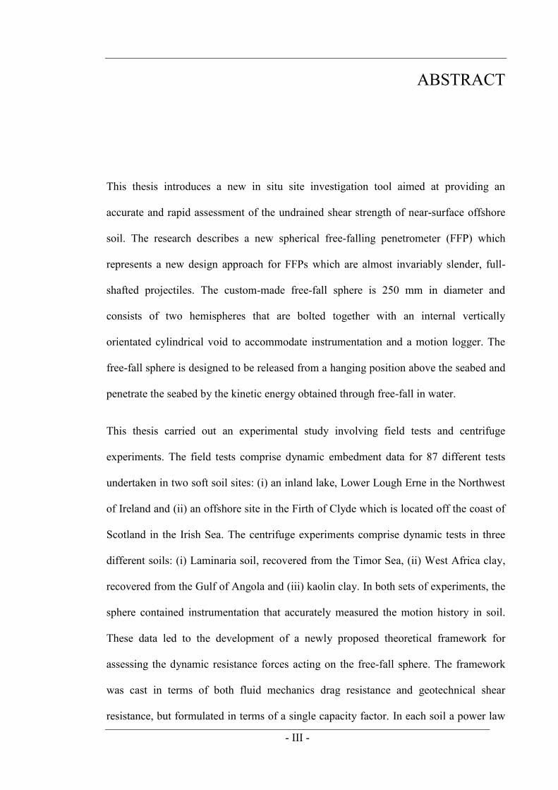
This thesis introduces a new in situ site investigation tool aimed at providing an
accurate and rapid assessment of the undrained shear strength of near-surface offshore
soil. The research describes a new spherical free-falling penetrometer (FFP) which
represents a new design approach for FFPs which are almost invariably slender, full-
shafted projectiles. The custom-made free-fall sphere is 250 mm in diameter and
consists of two hemispheres that are bolted together with an internal vertically
orientated cylindrical void to accommodate instrumentation and a motion logger. The
free-fall sphere is designed to be released from a hanging position above the seabed and
penetrate the seabed by the kinetic energy obtained through free-fall in water.
This thesis carried out an experimental study involving field tests and centrifuge
experiments. The field tests comprise dynamic embedment data for 87 different tests
undertaken in two soft soil sites: (i) an inland lake, Lower Lough Erne in the Northwest
of Ireland and (ii) an offshore site in the Firth of Clyde which is located off the coast of
Scotland in the Irish Sea. The centrifuge experiments comprise dynamic tests in three
different soils: (i) Laminaria soil, recovered from the Timor Sea, (ii) West Africa clay,
recovered from the Gulf of Angola and (iii) kaolin clay. In both sets of experiments, the
sphere contained instrumentation that accurately measured the motion history in soil.
These data led to the development of a newly proposed theoretical framework for
assessing the dynamic resistance forces acting on the free-fall sphere. The framework
was cast in terms of both fluid mechanics drag resistance and geotechnical shear
resistance, but formulated in terms of a single capacity factor. In each soil a power law

- IV -
function was adopted in order to account for the strain rate dependency. The
appropriateness of the strain rate parameter was demonstrated by varying β within the
typical range reported from variable rate penetrometer tests (β = 0.05 to 0.09). In the
field and centrifuge experiments, the best-fit rate parameter was calculated using β =
0.07.
To improve the strength characterisation of near surface seabeds with a shallowly-
embedded ball penetrometer or free-fall sphere, the thesis describes centrifuge
experiments designed to quantify the shallow penetration effects. The experiments were
carried out with an 11.3 mm diameter ball penetrometer penetrating kaolin clay under
undrained conditions over a range of normalised strength ratios, su/γ'D. The tests
captured the influence of two important mechanisms: (i) the varying soil buoyancy with
penetration depth and (ii) the reduced bearing factor, Nb-shallow, arising from the shallow
failure mechanism. The centrifuge results were combined with reinterpreted data from
LDFE analyses to form a unique relationship between the transition depth and the
normalised strength ratio over the range su/γ'D ≈ 0.07 to 40. This led to the development
of a shallow penetration framework to determine more accurately the undrained shear
strength of near surface soil.
Both frameworks described in the thesis represent significant advances in the
understanding of FFPs and when combined provide accurate estimation of the
undrained shear strength with the IFFS compared to a conventional ball penetrometer.
- V -
DECLARATION
This thesis is submitted as a series of papers within the regulations of the University of
Western Australia. The thesis contains published material and draft submissions that
have been prepared for publication. Unless otherwise stated, the candidate is responsible
for over 90% of the content in this thesis. The contribution of the candidate for the
papers described in Chapter 3–8 are defined as follows.
Chapter 3: Morton, J. P. & O‟Loughlin, C. D., 2012. Dynamic penetration of a
sphere in clay. Proceedings of the 7th International Conference on Offshore
Site Investigation and Geotechnics, London, UK, pp. 223–230.
The field tests and analysis of dynamic embedment in clay were performed
solely by the candidate. Both authors contributed to the publication of this
chapter after a full initial draft was provided by the candidate.
Chapter 4: Morton, J. P., O‟Loughlin, C. D. & White. D. J., 2014. Strength
assessment during shallow penetration of a sphere in clay. Géotechnique Letters
4 (October-December), pp. 262–266.
The candidate designed the centrifuge tests and carried out all physical
modelling experiments and interpreted all results. The paper was written by the
candidate after comments from the co-authors.
Chapter 5: O‟Loughlin, C. D., Gaudin, C., Morton. J. P. & White, D. J., 2014.
MEMS accelerometers for measuring dynamic penetration events in
geotechnical centrifuge tests International Journal of Physical Modelling in
Geotechnics, 14(2), pp. 31–39.
- VI -
The candidate led the data processing and interpretation of the experimental
data and produced a technical report that formed a basis for drafting the paper.
The estimated precent contribution of the author is 30%.
Chapter 6: Blake, A. P., O'Loughlin, C. D., Morton, J. P., O' Beirne, C., Gaudin,
C. & White, D. W., 2015. In-situ measurement of the dynamic penetration of
freefall projectiles in soft soils using a low cost inertial measurement unit.
Geotechnical Testing Journal, ASTM. DOI: 10.1520/GTJ20140135.
The field testing was performed in-part by the candidate along with some data
processing. The candidate was also involved in the data interpretation process;
the estimated precent contribution of the author is 20%.
Chapter 7: Morton, J. P., O‟Loughlin, C. D. & White. D. J., 2015. Field testing
an in situ freefalling spherical penetrometer in soft soil. Submitted to
Géotechnique.
The candidate carried out all field tests and analytical modelling in this paper.
The candidate also provided a detailed first draft that was revised after
comments from both co-authors.
Chapter 8: Morton, J. P., O‟Loughlin, C. D. & White. D. J., 2015. Centrifuge
modelling of an instrumented free-fall sphere for measurement of undrained
strength in fine grained soils. Canadian Geotechnical Journal. DOI:
10.1139/cgj-2015-0371
The candidate carried out all field tests and data interpretation in this paper and
produced the final submission draft after comments from the co-authors.

- VII -
The stated contributions have been agreed with the co-authors of each paper and
permission has been granted to include the relevant paper within this thesis.
John Morton, candidate………………………...…………………………………………
Conleth D O‟Loughlin, coordinating supervisor…………………….……………………

- VIII -
Contents
ABSTRACT .................................................................................................................. III
DECLARATION ............................................................................................................ V
LIST OF FIGURES .................................................................................................. XIII
LIST OF TABLES ..................................................................................................... XIX
ACKNOWLEDGEMENTS........................................................................................ XX
NOTATION ..................................................................................................................... 1
CHAPTER 1. INTRODUCTION .................................................................................. 7
1.1. RESEARCH MOTIVATIONS ......................................................................................... 7
1.2. THESIS OBJECTIVES ................................................................................................ 12
1.3. RESEARCH METHODOLOGY .................................................................................... 12
1.4. THESIS ORGANISATION ........................................................................................... 14
CHAPTER 2. REVIEW OF LITERATURE ............................................................. 19
2.1. INTRODUCTION ...................................................................................................... 19
2.2. IN SITU TOOLS ........................................................................................................ 19
2.2.1. In situ vane ..................................................................................................... 20
2.2.2. Cone and piezocone........................................................................................ 20
2.2.3. Full flow penetrometers.................................................................................. 21
2.2.3.1. T-bar and ball penetrometer ............................................................................... 23
2.2.4. Interpretation of shear strength from full flow penetrometers ....................... 24
2.2.5. Bearing capacity factor .................................................................................. 25
2.2.6. Interpretation of shear strength during shallow penetration ......................... 27
2.2.6.1. Transition depth .................................................................................................. 28
2.2.6.2. Wall failure ......................................................................................................... 28
2.2.6.3. Flow failure ........................................................................................................ 29
2.2.6.4. Bearing capacity factor variation with depth ..................................................... 32
2.2.6.5. Soil buoyancy ...................................................................................................... 32
- IX -
2.2.6.6. Operative depth .................................................................................................. 33
2.3. FREE-FALLING PENETROMETERS ............................................................................ 34
2.3.1. Free-falling penetrometer designs for naval mine countermeasure
applications .............................................................................................................. 34
2.3.2. Free-falling penetrometer designs for seabed characterisation .................... 37
2.3.3. FFP measurement systems ............................................................................. 39
2.3.3.1. Acoustic Doppler system .................................................................................... 39
2.3.3.2. Accelerometer system ......................................................................................... 39
2.3.4. Experimental and field studies on free-falling penetrometers ....................... 41
2.4. OCEANIC WASTE CARRIERS .................................................................................... 45
2.5. DYNAMICALLY INSTALLED ANCHORS .................................................................... 46
2.5.1. Experimental and field studies on dynamically installed anchors ................. 48
2.5.2. Centrifuge experiments ................................................................................... 50
2.6. RESISTANCE FORCES ACTING ON A PROJECTILE DURING DYNAMIC EMBEDMENT IN
SOIL .............................................................................................................................. 51
2.6.1. Fluid drag ....................................................................................................... 52
2.6.1.1. Drag in water ..................................................................................................... 53
2.6.1.2. Drag in soil ........................................................................................................ 56
2.6.2. Hydrodynamic mass force .............................................................................. 57
2.6.3. Strain rate effects in clay ................................................................................ 58
2.6.3.1. Strain rate parameter ......................................................................................... 60
2.6.3.2. Dependency of rate parameters on penetrometer geometry .............................. 62
2.6.3.3. Dependency of rate parameters on material properties .................................... 63
2.6.4. Combined fluid mechanics and soil mechanics framework ........................... 64
2.6.5. Unified framework .......................................................................................... 65
2.6.6. Analytical modelling ....................................................................................... 67
2.6.7. Numerical analysis ......................................................................................... 69
2.7. SUMMARY .............................................................................................................. 70
CHAPTER 3. DYNAMIC PENETRATION OF A SPHERE IN CLAY ................. 72
3.1. ABSTRACT ............................................................................................................. 72
3.2. INTRODUCTION ...................................................................................................... 73
3.3. SITE DESCRIPTION AND SOIL PROPERTIES ............................................................... 74
3.3.1. Site location and description .......................................................................... 74
3.3.2. Soil classification ........................................................................................... 74

- X -
3.3.3. Shear strength profiles ................................................................................... 75
3.4. TEST EQUIPMENT AND TESTING PROCEDURES ........................................................ 76
3.4.1. Instrumented free-fall sphere ......................................................................... 76
3.4.2. Motion logger ................................................................................................. 77
3.4.3. Field testing procedure .................................................................................. 78
3.5. TEST RESULTS AND ANALYSIS ................................................................................ 78
3.5.1. Acceleration profile ........................................................................................ 78
3.5.2. Acceleration profile interpretation ................................................................. 81
3.5.3. Velocity and embedment depth profile ........................................................... 82
3.6. EMBEDMENT DEPTH PREDICTION ........................................................................... 82
3.7. CONCLUSIONS ........................................................................................................ 89
CHAPTER 4. STRENGTH ASSESSMENT DURING SHALLOW
PENETRATION OF A SPHERE IN CLAY .............................................................. 90
4.1. ABSTRACT ............................................................................................................. 90
4.2. INTRODUCTION ...................................................................................................... 91
4.3. EXPERIMENTAL DETAILS ........................................................................................ 92
4.4. EXPERIMENTAL PROCEDURE .................................................................................. 93
4.4.1. Preparation of clay specimen ......................................................................... 93
4.5. THEORETICAL BASIS FOR INTERPRETATION OF MEASURED BALL PENETRATION
RESISTANCE .................................................................................................................. 96
4.6. RESULTS AND COMPARISONS ............................................................................... 100
4.6.1. In-flight video camera observations ............................................................. 100
4.6.2. Undrained shear strength profiles ............................................................... 101
4.6.3. Deep mechanism transition depth ................................................................ 102
4.6.4. Shallow bearing capacity factors ................................................................. 103
4.7. CONCLUSIONS ...................................................................................................... 104
CHAPTER 5. MEMS ACCELEROMETERS FOR MEASURING DYNAMIC
PENETRATION EVENTS IN GEOTECHNICAL CENTRIFUGE TESTS ........ 106
5.1. ABSTRACT ........................................................................................................... 106
5.2. INTRODUCTION .................................................................................................... 107
5.3. STATIC CENTRIFUGE TESTS .................................................................................. 111
5.4. EXAMPLE APPLICATION: DYNAMICALLY INSTALLED ANCHORS ............................ 115
5.5. DYNAMIC CENTRIFUGE TESTS .............................................................................. 117

- XI -
5.6. INTERPRETATION OF ACCELEROMETER DATA ....................................................... 122
5.7. CONCLUDING REMARKS ....................................................................................... 130
CHAPTER 6. IN-SITU MEASUREMENT OF THE DYNAMIC PENETRATION
OF FREE FALL PROJECTLES IN SOFT SOILS USING A LOW COST
INERTIAL MEASUREMENT UNIT ....................................................................... 131
6.1. ABSTRACT ........................................................................................................... 131
6.2. INTRODUCTION .................................................................................................... 132
6.3. FREE-FALLING PROJECTILES ................................................................................. 136
6.3.1. Deep penetrating anchors ............................................................................ 136
6.3.2. Dynamically embedded plate anchors ......................................................... 137
6.3.3. Instrumented free-falling sphere .................................................................. 138
6.3.4. Inertial measurement unit ............................................................................ 139
6.4. INTERPRETATION OF IMU MEASUREMENTS ......................................................... 141
6.4.1. Rotation ........................................................................................................ 142
6.4.2. Acceleration .................................................................................................. 144
6.4.3. Velocity and distance .................................................................................... 146
6.4.4. Tilt angles ..................................................................................................... 147
6.5. TEST SITES AND SOIL PROPERTIES ........................................................................ 147
6.6. TEST PROCEDURE ................................................................................................. 150
6.7. RESULTS AND DISCUSSION ................................................................................... 153
6.7.1. Rotation ........................................................................................................ 153
6.7.2. Acceleration .................................................................................................. 157
6.7.3. Velocity profiles ............................................................................................ 160
6.7.4. Verification of the IMU derived measurements ........................................... 163
6.7.5. Example application of projectile IMU data ................................................ 164
6.8. CONCLUSIONS ...................................................................................................... 168
CHAPTER 7. ESTIMATION OF SOIL STRENGTH BY INSTRUMENTED
FREE-FALL SPHERE TESTS .................................................................................. 170
7.1. ABSTRACT ........................................................................................................... 170
7.2. INTRODUCTION .................................................................................................... 171
7.3. BEARING CAPACITY FACTOR ................................................................................ 174
7.4. SITE DESCRIPTION AND SOIL PROPERTIES ............................................................. 175
7.5. TEST EQUIPMENT AND TESTING PROCEDURES ...................................................... 178

- XII -
7.5.1. Instrumented free-fall sphere ....................................................................... 178
7.5.2. Inertial measurement unit ............................................................................ 178
7.5.3. Field testing procedure ................................................................................ 180
7.6. FORCES ACTING ON A SPHERE DURING FREE-FALL IN WATER ............................... 184
7.7. FORCES ACTING ON A SPHERE DURING DYNAMIC PENETRATION IN SOIL ............... 188
7.8. SOIL STRENGTH ESTIMATION USING FREE-FALL SPHERE DATA ............................. 193
7.9. CONCLUSIONS ...................................................................................................... 196
CHAPTER 8. CENTRIFUGE MODELLING OF AN INSTRUMENTED FREE-
FALL SPHERE FOR MEASUREMENT OF UNDRAINED STRENGTH IN
FINE-GRAINED SOILS ............................................................................................ 197
8.1. ABSTRACT ........................................................................................................... 197
8.2. INTRODUCTION .................................................................................................... 198
8.3. PENETRATION OF A SPHERE IN SOIL ...................................................................... 202
8.4. EXPERIMENTAL DETAILS ...................................................................................... 206
8.4.1. Measurement technique ................................................................................ 206
8.4.2. Instrumented free-fall sphere ....................................................................... 209
8.4.3. Soil preparation technique ........................................................................... 210
8.4.4. Centrifuge test details and procedures ......................................................... 210
8.5. TEST RESULTS AND DISCUSSION ........................................................................... 212
8.5.1. Penetrometer tests and soil properties ......................................................... 212
8.5.2. Free-fall tests ................................................................................................ 216
8.5.3. Interpretation of free-fall acceleration data ................................................ 222
8.6. CONCLUSION ........................................................................................................ 230
CHAPTER 9. CONCLUSIONS ................................................................................. 232
9.1. SUMMARY ............................................................................................................ 232
9.2. MAIN FINDINGS .................................................................................................... 234
9.2.1. Free-fall and dynamic embedment in soil .................................................... 234
9.2.2. MEMS accelerometers in the centrifuge ...................................................... 235
9.2.3. Shallow penetration framework ................................................................... 236
REFERENCES ............................................................................................................ 239

- XIII -
LIST OF FIGURES
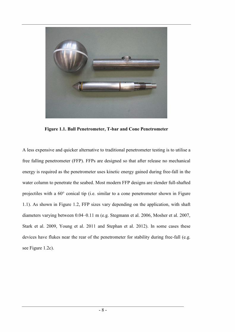
Figure 1.1. Ball Penetrometer, T-bar and Cone Penetrometer .......................................... 8
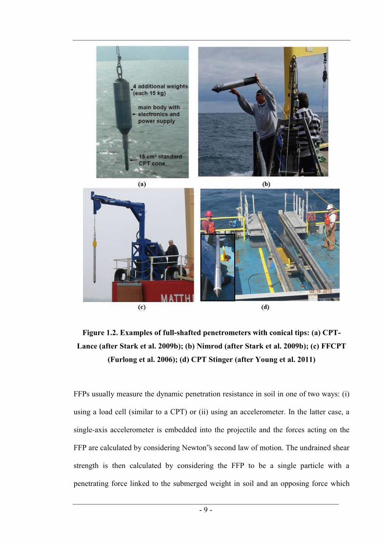
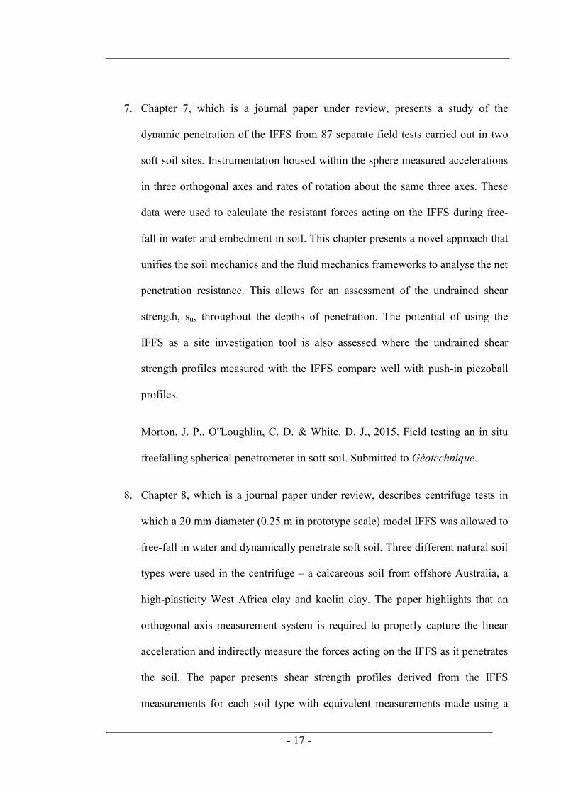
Figure 1.2. Examples of full-shafted penetrometers with conical tips: (a) CPT-Lance
(after Stark et al. 2009b); (b) Nimrod (after Stark et al. 2009b); (c) FFCPT (Furlong
et al. 2006); (d) CPT Stinger (after Young et al. 2011) .............................................. 9
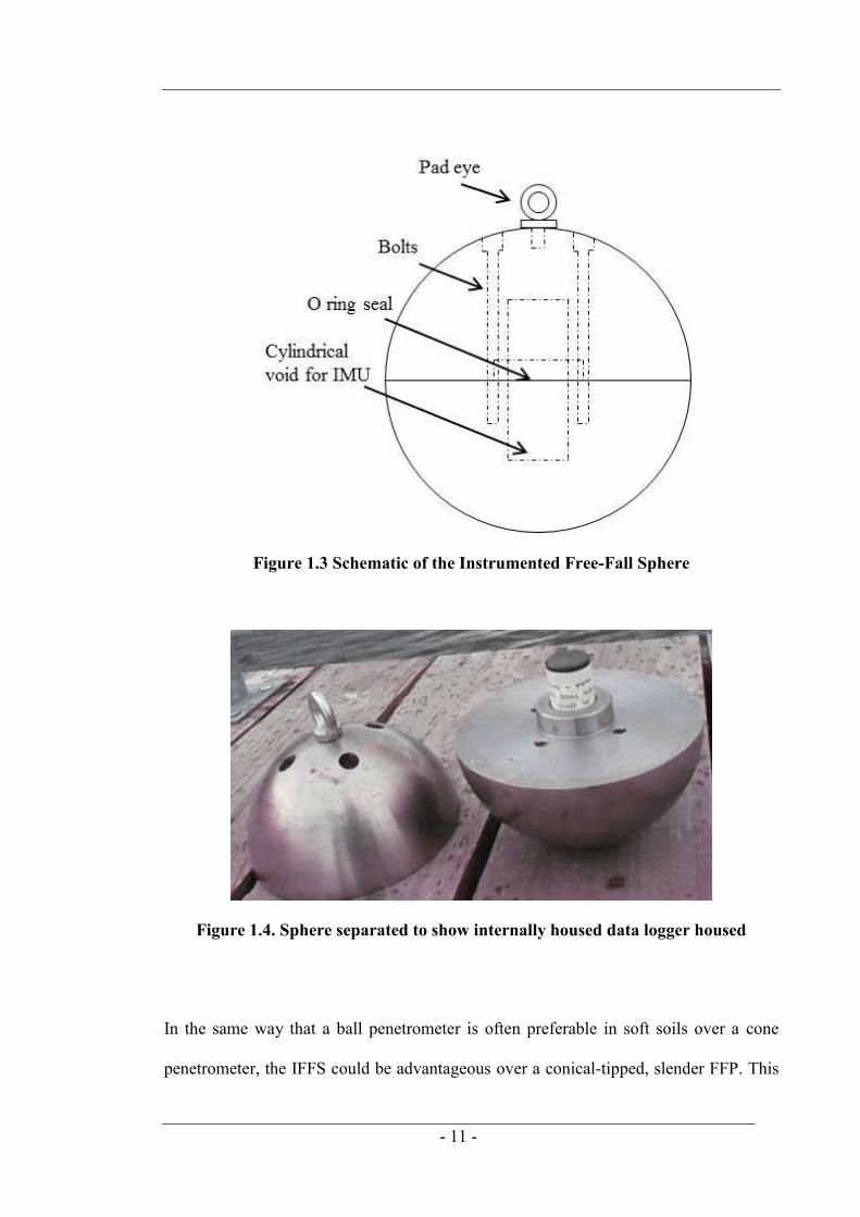
Figure 1.3 Schematic of the Instrumented Free-Fall Sphere........................................... 11
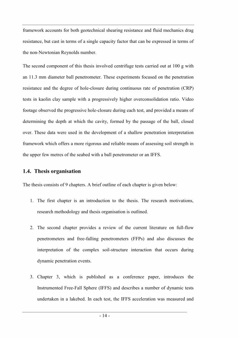
Figure 1.4. Sphere separated to show internally housed data logger housed .................. 11
Figure 2.1. (a) T-bar; (b) Ball penetrometer ................................................................... 23
Figure 2.2. Soil failure mechanism for a ball penetration in uniform clay (Zhou et al.
2013) ......................................................................................................................... 30
Figure 2.3. The effect of su/γ‟D on the transition depth for a ball penetrometer (after
Zhou et al. 2013) ...................................................................................................... 31
Figure 2.4. FFPs developed for naval mine countermeasure studies (a) XDP
(www.sonatech.com), (b) STING (after Abelev et al. 2009b) (c) ESP (after
Mulhearn et al. 1998), (d) BMMB (after Chow 2013), (e) AUSSI (after Mulhearn et
al. 1999), (f) FEP (after Chow 2013) and (g) PROBOS (after Stoll et al. 2007) ..... 36
Figure 2.5. FFP systems developed for applications in seabed characterisation (a)
Marine Impact Penetrometer (after Dayal et al. 1975), (b) MSP-2 (after Colp et al.
1975), (c) Freefall penetrometer (after Denness et al. 1981), (d) XBP (after Stoll &
Akal 1999), (e) FFCPT (www.brooke-ocean.com), (f) LIRmeter (after Stephan et
al. 2012), (g) CPT-Lance (after Stark et al. 2009b), (h) Nimrod (after Stark et al.
2009b), (i) CPT Stinger (after Young et al. 2011) ................................................... 38
Figure 2.6. Typical velocity and penetration depth with time profiles for the FFP
instrumented with an accelerometer (Chow & Airey 2010b) .................................. 41
Figure 2.7. Acceleration profile in soil (after Stephan et al. 2012) ................................. 41
Figure 2.8. Cone tip resistance of the PROBOS compared to the STATPEN, a quasi-
static cone penetrometer (after Stoll et al. 2007) ...................................................... 43
Figure 2.9. (a) Different tip designs for the STING; (b) Tip diameter effect in
interpreted soil strength for the STING (after Abelev et al. 2009b) ........................ 44

- XIV -
Figure 2.10. The European Standard Penetrometer (Freeman & Burdett, 1986) ........... 46
Figure 2.11. Dynamically installed anchors (Medeiros, 2002); (b) Torpedo Anchor
(Brandão et al. 2006) ................................................................................................ 48
Figure 2.12. (a) Forces acting on a full-shafted penetrometer and (b) Thin-shafted
penetrometer during installation ............................................................................... 52
Figure 2.13. Drag coefficient for uniform flow past a sphere R = Re < 2 x 10⁵ (480 data
points) after (Brown & Lawler 2003) ....................................................................... 54
Figure 2.14. Drag coefficient for uniform flow past a sphere Re > 2 x 10⁵ (Achenbach,
1972) ......................................................................................................................... 55
Figure 2.15. Laminar-separated flow and turbulent flow over a sphere - (after
Finnemore & Franzini 2001) .................................................................................... 56
Figure 2.16. Normalised velocity illustration (after Lehane et al. 2009) ........................ 59
Figure 2.17. Variation in back-analysed β and λ strain rate parameters with impact
velocity for reduced scale model DPAs from centrifuge experiments in kaolin clay
(after O‟Loughlin et al. 2013b) ................................................................................ 61
Figure 2.18. Variation of normalised lateral pressure on a pipe with non-Newtonian
Reynolds number ...................................................................................................... 66
Figure 3.1. Site location and bathymetric map of Lower Lough Erne (after Lafferty et al.
2006) ......................................................................................................................... 74
Figure 3.2. Typical undrained shear strength profiles at the test site .............................. 76
Figure 3.3. (a) sphere separated to show internally housed data logger housed, (b)
motion logger and underwater housing, (c) sphere suspended over the water prior to
a drop ........................................................................................................................ 77
Figure 3.4. (a) x, y and z axis acceleration traces from a typical test, (b) x and y axis
rotation traces from the same test ............................................................................. 80
Figure 3.5. z axis acceleration trace for the test shown on Figure 3.4 together with
corresponding velocity and displacement traces ...................................................... 81
Figure 3.6. Velocity profiles in water and soil for release heights of 0.5 m and 1 m ..... 83
Figure 3.7. Measuring the embedment depth using markers on the retrieval rope taken
with the underwater camera ..................................................................................... 84
Figure 3.8. Forces acting on the IFFS during penetration in soil.................................... 84
Figure 3.9. Measured and theoretical velocity profiles of the sphere free-falling in water
.................................................................................................................................. 87

- XV -
Figure 3.10. Predicted and measured velocity profiles of the sphere penetrating the
lakebed ...................................................................................................................... 89
Figure 4.1. (a) and (b) Experimental arrangement in the beam centrifuge ..................... 94
Figure 4.2. A scraped soil sample before a test .............................................................. 95
Figure 4.3. Ball penetrometer and cavity after a penetration test ................................... 95
Figure 4.4. Schematic illustration of soil buoyancy due to (a) the sphere and (b) the
sphere and conical cavity (c) buoyancy function for a typical cavity depth ............ 98
Figure 4.5. Comparison of strength profiles from Equation 4.4 and qnet/Nb-deep ........... 100
Figure 4.6. Effect of strength ratio su/γ'D on transition depth ....................................... 103
Figure 4.7. Measured variation in normalised bearing factor with normalised
embedment depth and equation fit ......................................................................... 104
Figure 5.1. Schematic representation of the operational principle of a MEMS
accelerometer .......................................................................................................... 109
Figure 5.2. MEMS accelerometer: (a) Analog Devices ADXL001 MEMS accelerometer
with an internal view of the chip showing the MEMS sensor surrounded by the
integrated circuitry and (b) Scanning Electron Microscope image of the ADXL001
accelerometer showing the proof mass, plates, springs and anchor points ............ 110
Figure 5.3. Comparison between MEMS acceleration measurements and those derived
from the rotational speed of the centrifuge during spin up to 100 g and down again:
(a) time history, and (b) comparison ...................................................................... 113
Figure 5.4. Comparison between position measurements derived from the MEMS
accelerometer and measured using the motor encoder on the vertical axis of the
actuator ................................................................................................................... 115
Figure 5.5. Dynamically installed anchors: (a) torpedo pile (after Araujo et al. 2004), (b)
OMNI-Max anchor (after Shelton, 2007), (c) deep penetrating anchor (Deep Sea
Anchors, www.deepseaanchors.com/News.html) .................................................. 116
Figure 5.6. Accelerometers installed in a model dynamically installed anchor ............ 117
Figure 5.7. Dynamic anchor experimental arrangement showing the anchor located in
installation guide before release and embedded in the soil sample after release ... 119
Figure 5.8. MEMS and piezoelectric accelerometer data measured before, during and
after a dynamically installed anchor drop in a beam centrifuge: (a) entire trace, (b)
during freefall and embedment ............................................................................... 120

- XVI -
Figure 5.9. Interpretation of the MEMS accelerometer data in the rotating frame of
reference: (a) acceleration, velocity and displacement traces, (b) velocity profile
during freefall and embedment............................................................................... 124
Figure 5.10. Anchor velocity profiles for an anchor installation in kaolin clay with su =
1.1z ......................................................................................................................... 126
Figure 5.11. Effect of anchor tilt during embedment in soil (kaolin clay with su = 1.1z):
(a) 5 degree tilt, (b) 10 degree tilt, (c) 20 degree tilt, (d) 30 degree tilt ................. 129
Figure 6.1. Schematic representation of the operational principle of: (a) MEMS
accelerometers and (b) MEMS gyroscopes ............................................................ 134
Figure 6.2. Deep penetrating anchor ............................................................................. 137
Figure 6.3. Dynamically embedded plate anchor ......................................................... 138
Figure 6.4. Instrumented free-falling sphere ................................................................. 139
Figure 6.5. Inertial Measurement Unit .......................................................................... 140
Figure 6.6. Body frame of reference ............................................................................. 141
Figure 6.7. Resultant tilt angle, μ, defined in the inertial frame ................................... 142
Figure 6.8. Test sites locations ...................................................................................... 149
Figure 6.9. Undrained shear strength profiles: (a) Firth of Clyde and (b) Lough Erne 150
Figure 6.10. (a) RV Aora and (b) Self-propelled barge ................................................ 151
Figure 6.11. DEPLA field test procedure ..................................................................... 152
Figure 6.12. Image capture from ROV camera showing the follower retrieval line at the
seabed ..................................................................................................................... 153
Figure 6.13. Projectile rotations during free-fall through water and soil penetration: (a)
DEPLA, (b) IFFS and (c) DPA .............................................................................. 156
Figure 6.14. Projectile accelerations during free-fall through water and soil penetration:
(a) DEPLA, (b) IFFS and (c) DPA ......................................................................... 159
Figure 6.15. Projectile velocity profiles corresponding to free-fall through water and soil
penetration: (a) DEPLA, (b) IFFS and (c) DPA ..................................................... 162
Figure 6.16. Comparision of IMU derived displacement measurements with those
obtained using a draw wire sensor ......................................................................... 164
Figure 6.17. DEPLA velocity profile derived from the IMU data measured at the Firth
of Clyde test site and corresponding theoretical profile ......................................... 168
Figure 7.1. Undrained shear strength profiles in: (a) Lough Erne and (b) Firth of Clyde
................................................................................................................................ 177
- XVII -
Figure 7.2. Instrumented free-fall sphere: (a) sphere separated with IMU located within
internal void, (b) IMU and (c) assembled sphere prior to a free-fall test in Erne .. 178
Figure 7.3 IMU measurements and their interpretation from a typical free-fall sphere
test in Erne .............................................................................................................. 180
Figure 7.4. Forces acting on a sphere: (a) free-falling in water, (b) during dynamic
penetration in soil ................................................................................................... 186
Figure 7.5. Measured and theoretical evolution of the drag coefficient, CD, during free-
fall in water ............................................................................................................. 188
Figure 7.6. Relationship between N and Renon-Newtonian for: (a) Erne and (b) Clyde ..... 192
Figure 7.7. Comparison of undrained shear strength profiles derived from free-fall
sphere acceleration data and push-in piezoball penetration resistance: (a) Erne and
(b) Clyde ................................................................................................................. 195
Figure 8.1. Examples of free-fall shafted penetrometers with conical tips:(a) CPT-Lance
(courtesy of Dr. Nina Stark); (b) Nimrod (courtesy of Dr. Nina Stark); (c) FFCPT
(Furlong et al. 2006); (d) CPT Stinger (after Young et al. 2011) ........................... 200
Figure 8.2. Free-fall sphere ready for release (Morton and O‟Loughlin 2012) ............ 200
Figure 8.3. Forces acting on the sphere during penetration in soil ............................... 202
Figure 8.4. Model instrumented sphere shown: (a) during fabrication showing the void
in the sphere for the tri-axis MEMS accelerometer (b) after fabrication alongside a
centrifuge scale push-in ball penetrometer ............................................................. 208
Figure 8.5. Experimental arrangement for the push-in ball and instrumented free-fall
sphere tests ............................................................................................................. 211
Figure 8.6. Profiles of: (a) undrained shear strength with depth (from ball penetrometer
tests) and (b) moisture content and effective unit weight with depth established
from post-testing sample cores ............................................................................... 215
Figure 8.7. Accelerometer, velocity and displacement traces in a typical free-fall sphere
centrifuge test in kaolin clay................................................................................... 218
Figure 8.8. Example time histories of: (a)linear acceleration, (b) velocity and (c)
displacement for the three soil types ...................................................................... 220
Figure 8.9. Post-test analysis of the sphere trajectory and measurement of the final
embedment depth ................................................................................................... 222
Figure 8.10. Relationship between N and Renon-Newtonian for a sphere in the three soil
types: (a) Laminaria soil (b) West Africa clay (c) kaolin ....................................... 224

- XVIII -
Figure 8.11. su profiles from free-fall sphere and push-in penetrometer tests in: (a)
Laminaria soil (b) West Africa soil (c) kaolin ....................................................... 229
Figure 8.12. Effect of varying β parameter on free-fall sphere su profile ..................... 230
Figure 9.1. The formulation of the centroidal height for an invert depth < 0.5D ......... 274
Figure 9.2. The formulation of the centroidal height for an invert depth > 0.5D ......... 274

- XIX -
LIST OF TABLES
Table 7.1. Free-fall sphere test data from the Erne tests ............................................... 182
Table 7.2. Free-fall sphere test data from the Clyde tests ............................................. 184
- XX -
ACKNOWLEDGEMENTS
I would like to take this opportunity to sincerely thank my supervisors Dr. Conleth
O‟Loughlin and Professor David White. Thank you for your guidance, patience and
energy throughout this PhD, it has been invaluable.
To my colleagues in the Centre for Offshore Foundation Systems (COFS) UWA, thank
for your assistance and technical expertise and insights with regard to the experimental
work presented in this thesis. A special thanks to the soils and centrifuge laboratory and
workshop staff, in particular John Breen, Manuel Palacios, Kelvin Leong, Khin Seint,
Dave Jones and Shane De Catania. Your technical support and team attitude has made
the testing component one of the most enjoyable aspects of my research.
The financial support provided an Australian Postgraduate Award, Scholarship for
International Research Fees and COFS Top Up Scholarship is gratefully acknowledged.
Thank you to my colleagues and friends Janice Brogan, Cathal Colreavy, Anthony
Blake, Colm O‟Beirne, Michael Cocjin, Chao Han, Emma Leitner, Raffaele Ragni,
Henning Mohr, Simon Leckie, Fillippo Gaone, Lisa Melvin, Shiaohuey Chow, Cristina
Vulpe and Joe Tom JR. I am thankful for your consideration and the friendship we have
developed over the past four years. Thank you for the kindness, honesty and sense of
humour that you have all provided.
Finally, and most importantly, I would like to thank my family - Joan and Gary, Scott,
Gary JR, Claire and Grandparents John Flood and Iris Morton. Thank you for you open
minded attitude towards my research and thank you for you relentless love and warmth.
Without your continual support and encouragement I would not be the positive person I
am today.

- 1 -
NOTATION
Roman
a resultant linear acceleration
abz linear acceleration coincident with the body frame z-axis
aix linear acceleration coincident with the inertial frame x-axis
aiy linear acceleration coincident with the inertial frame y-axis
aiy linear acceleration coincident with the inertial frame x-axis
A acceleration measurement
Abx acceleration measurement coincident with the body frame x-axis
Aby acceleration measurement coincident with the body frame y-axis
Abz acceleration measurement coincident with the body frame z-axis
ADC analogue to digital converter
Ax acceleration measurement coincident with the inertial frame x-axis
Ay acceleration measurement coincident with the inertial frame y-axis
Az acceleration measurement coincident with the inertial frame z-axis
Ap frontal/projected area
Ar resultant linear acceleration
As surface area
ch horizontal coefficient of consolidation
cv vertical coefficient of consolidation
Cm added mass coefficient
CD drag coefficient
D diameter
dt change in time
FAM added mass force
Fbuoy soil buoyancy force
Fb bearing resistance force
Fd fluid drag resistance force
Ffrict frictional resistance force
Fresist combined resistance force
- 2 -
FSS submerged weight in soil
g gravitational acceleration
hiz,drop drop height derived from the inertial frame acceleration and rotation measurements
Hc height of the conical cavity
Hw cavity depth
k undrained shear strength gradient
m mass
m' added mass
N bearing capacity factor
Nball ball penetrometer/ piezoball bearing capacity factor
Nb-shallow reduced bearing factor
Nc bearing capacity factor
Nc,deep maximum bearing capacity factor
Nkt piezocone bearing capacity factor
NT-bar T-bar bearing capacity factor
n, nl strain rate parameters
qm measured penetration resistance
Rbi direction cosine matrix (body frame to inertial frame)
Re Reynolds number for a Newtonian fluid
Renon-Newtonian Reynolds number for a non-Newtonian fluid
Re effective radius
Rf strain rate function
Rf,frict strain rate factor for shaft resistance
Rf,bear strain rate factor for tip resistance
Rx roll matrix
Ry pitch matrix
Rz yaw matrix
s distance travelled in the direction of motion
s0 initial distance travelled in the direction of motion
sbz vertical distance travelled coincident with the body-frame
sz vertical distance travelled coincident with the inertial-frame
sz0 initial vertical distance travelled coincident with the inertial-frame
su undrained shear strength
su,op operative undrained shear strength
St soil sensitivity
- 3 -
t time
Tbi angular velocity transformation matrix (body frame to inertial frame)
v velocity
vbz velocity coincident with the body frame z-axis
vi impact velocity
vix velocity coincident with the inertial frame x-axis
viy velocity coincident with the inertial frame y-axis
viz velocity coincident with the inertial frame z-axis
vix,0 initial velocity coincident with the inertial frame x-axis
viy,0 initial velocity coincident with the inertial frame y-axis
viz,0 initial velocity coincident with the inertial frame z-axis
V non-dimensional velocity
VS full scale voltage output range
VADC full scale input voltage range of analogue to digital converter
Vdisp volume of the displaced soil
Ws submerged weight
w ball invert depth
ŵop normalised operative depth
ŵdeep-op normalised transition depth
xb body frame x-axis
xi inertial frame x-axis
yb body frame y-axis
yi inertial frame y-axis
z embedment depth (for keying and capacity) or travel distance (free-fall in water and dynamic embedment in soil)
zb body frame z-axis
zi inertial frame z-axis
ziz vertical distance travelled (coincident with the inertial frame)
ziz,e embedment depth (coincident with the inertial frame)
zs separation depth
Greek α adhesion factor
β strain rate parameter (power law)
γ unit weight
γ' effective unit weight of soil
- 4 -
γ strain rate
γref reference strain rate
δrem ratio of fully remoulded strength to intact soil strength
η soil viscosity parameter
θ pitch angle
θb pitch angle coincident with the body frame
θi pitch angle coincident with the inertial frame
θi,acc pitch angle coincident with the inertial frame (derived from accelerometer measurement)
∆N minimum resolvable acceleration resolution
∆R minimum displacement resolution
Δze difference between measured and predicted embedment depth
λ strain rate parameter (semi-logarithmic law)
ν dynamic viscosity
μ strain rate parameter
μ' resultant tilt angle (relative to Earth‟s gravity)
ξ95 accumulated absolute plastic shear strain rate for the 95% remoulding
π ratio of a circle‟s circumference to its diameter
ρ fluid/soil density
σ'v vertical effective stress
τ shear stress
τy shear yield stress
ψb yaw angle coincident with the body frame
ψi yaw angle coincident with the inertial frame
ωbx rotation rate about the body frame x-axis
ωby rotation rate about the body frame y-axis
ωbz rotation rate about the body frame z-axis
ωix rotation rate about the inertial frame x-axis
ωiy rotation rate about the inertial frame y-axis
ωiz rotation rate about the inertial frame z-axis
ϕ roll angle
ϕb roll angle coincident with the body frame
ϕb0 initial roll angle coincident with the body frame
ϕi roll angle coincident with the inertial frame
ϕi,acc roll angle coincident with the inertial frame (derived from accelerometer measurement)
- 5 -
Abbreviations
ALE Arbitrary Lagrangian-Eulerian
AUSSI Australian Underwater Sediment Strength Instrument
AVTM Angular Velocity Transformation Matrix
BMMP Burying Mock Mine Body
CEL Coupled Eulerian-Lagrangian
CFD Computational Fluid Dynamics
CPT Cone Penetrometer Test
CRP Continous Rate Penetration
DCM Directional Cosine Matrix
DEPLA Dynamically Embedded PLate Anchor
DoF Degrees of Freedom
DPA Deep Penetrating Anchor
ESP European Standard Penetrometer
FEP FAU Experimental Penetrometer
FFCPT Free-Falling Cone Penetrometer Test
FFP Free-Falling Penetrometer
FPSO Floating, Production, Storage and Offloading
GB Giga Byte
GME Great Meteor East
GOM Gulf of Mexico
IFFS Instrumented Free-Falling Sphere
IMU Inertial Free-Falling Sphere
LDFE Large Deformation Finite Element
LIR Lance Insertion Rod
LL Liquid Limit
MEMS Micro Electro Mechanical System
MIP Marine Impact Penetrometer
MODU Mobile Offshore Drilling Unit
MSP Marine Sediment Penetrometer
NAP Nares Abyssal Plain
OCR Over Consolidation Ratio
PERP Photo emitter Receiver Pair
PROBOS Proboscis

- 6 -
RITSS Remeshing and Interpolation Technique with Small Strain
SEM Scanning Electron Microscope
STING Seabed Terminal Impact Naval Gauge
UWA University of Western Australia
XBP eXpendable Bottom Penetrometer
XDP eXpendale Doppler Penetrometer
- 7 -
CHAPTER 1. INTRODUCTION
1.1. Research motivations
The progression of the offshore energy industry has led to operation in very deep water,
approaching 3000 metres. This has driven the transition from fixed platforms to floating
production facilities which has led to an increased use of subsea facilities such as
flowlines, pipelines and mudmats. The geotechnical design of these infrastructures
requires the precise assessment of the undrained shear strength (su) in the near-surface
soil which is often limited to the upper 1–2 metres and in the case of pipelines, even the
upper 0.5 m (Randolph & White 2008). Offshore soil is often fine-grained and
normally-consolidated with very low strength (< 10 kPa) at the surface with an
increasing strength with depth (1–2 kPa/m). Characterisation of these soils is
challenging, and usually incorporates in situ testing due to the difficulty of recovering
high quality samples in deep water. In situ testing requires the deployment of a large
submersible penetration rig that is lowered to the seabed where a cone penetrometer, T-
bar or ball penetrometer (Figure 1.1) is driven into the soil at a constant rate of 20 mm/s.
The costs associated with these in situ, quasi-static penetration tests are significant and
increase with water depth.
- 8 -
Figure 1.1. Ball Penetrometer, T-bar and Cone Penetrometer
A less expensive and quicker alternative to traditional penetrometer testing is to utilise a
free falling penetrometer (FFP). FFPs are designed so that after release no mechanical
energy is required as the penetrometer uses kinetic energy gained during free-fall in the
water column to penetrate the seabed. Most modern FFP designs are slender full-shafted
projectiles with a 60° conical tip (i.e. similar to a cone penetrometer shown in Figure
1.1). As shown in Figure 1.2, FFP sizes vary depending on the application, with shaft
diameters varying between 0.04–0.11 m (e.g. Stegmann et al. 2006, Mosher et al. 2007,
Stark et al. 2009, Young et al. 2011 and Stephan et al. 2012). In some cases these
devices have flukes near the rear of the penetrometer for stability during free-fall (e.g.
see Figure 1.2c).
- 9 -
Figure 1.2. Examples of full-shafted penetrometers with conical tips: (a) CPT-
Lance (after Stark et al. 2009b); (b) Nimrod (after Stark et al. 2009b); (c) FFCPT
(Furlong et al. 2006); (d) CPT Stinger (after Young et al. 2011)
FFPs usually measure the dynamic penetration resistance in soil in one of two ways: (i)
using a load cell (similar to a CPT) or (ii) using an accelerometer. In the latter case, a
single-axis accelerometer is embedded into the projectile and the forces acting on the
FFP are calculated by considering Newton‟s second law of motion. The undrained shear
strength is then calculated by considering the FFP to be a single particle with a
penetrating force linked to the submerged weight in soil and an opposing force which

- 10 -
comprises the reaction force (i.e. the mass multiplied by linear acceleration) and various
other resistance forces linked in part to the undrained shear strength. One of the most
attractive properties of a FFP is the ease and speed of installation compared to
traditional penetrometers. For example, the penetrometer shown in Figure 1.2c can be
deployed from a constantly moving vessel. This allows a survey a FFP to cover a large
seabed area in a relatively short period of time. This can reduce the cost of seabed
surveys and improve the quantification of spatial variability.
Despite a number of successful FFP field trials undertaken since the 1960s, their
application is not widespread. This is partly due to uncertainties regarding the strain rate
effects in soil and also due to the interpretation of the undrained shear strength which
requires the definition of a bearing capacity factor, Nc. This is traditionally difficult to
ascertain for a conical tipped penetrometer and many numerical and empirical
correlations vary widely (Aubeny & Shi 2006, Nazem et al. 2012, Lunne et al. 1997).
Further uncertainties exist in relation to the frictional resistance generated along the
shaft and the different strain rate dependency of the penetrometer shaft compared to the
tip (Dayal et al. 1975, Steiner et al. 2014).
With these concerns in mind, this thesis introduces a new FFP known as the
Instrumented Free-Fall Sphere (IFFS) which represents a step change compared to the
traditional full-shafted, slender FFPs. The IFFS used in this study is a custom-made,
250 mm diameter mild steel sphere that consists of two hemispheres that are bolted
together with an internal vertically-orientated cylindrical void to accommodate
instrumentation that measures the motion history in water and soil (Figure 1.3 and
Figure 1.4). The sphere and instrumentation weighs 620N in air and has a submerged
weight of 549N in water. Attached to the padeye of the sphere is a retrieval line that is
used for deploying and recovering the IFFS after penetration in soil.
- 11 -
Figure 1.3 Schematic of the Instrumented Free-Fall Sphere
Figure 1.4. Sphere separated to show internally housed data logger housed
In the same way that a ball penetrometer is often preferable in soft soils over a cone
penetrometer, the IFFS could be advantageous over a conical-tipped, slender FFP. This

- 12 -
is because more closely-bracketed plasticity solutions are available for deducing shear
strength from the net penetration resistance of a ball penetrometer compared to a cone
(Randolph & Houlsby 1984, Randolph et al. 2000, Einav & Randolph. 2005). Therefore,
this thesis, for the first time, considers the merit of the IFFS through a set of centrifuge
and field tests and compares the performance to push-in ball penetrometer tests in
numerous soil types.
1.2. Thesis objectives
The main objective of this thesis is to examine the potential for the IFFS to be used as a
tool for measuring the undrained shear strength of near-surface, fine-grained soils.
Encompassed within this main objective are the following specific objectives:
To investigate the performance of the IFFS in a range of soil types through a
series of offshore field tests and physical modelling experiments in a
geotechnical centrifuge.
To develop frameworks that improve the interpretation of the undrained shear
strength from the IFFS measured penetration resistance.
To demonstrate the merit of the tool and the associated interpretative
frameworks by comparing the shear strength profiles derived from the IFFS
with corresponding data obtained from well-calibrated push-in ball
penetrometer tests.
1.3. Research methodology
This thesis comprises two major components – a dynamic penetration component
studying the complex processes associated with the embedment of an Instrumented
Free-Fall Sphere (IFFS) and also a continuous rate penetration (CRP) component
studying shallow penetration effects of a shallowly-embedded ball penetrometer in

- 13 -
kaolin clay. The experimental studies involve field tests and physical modelling
experiments using a geotechnical centrifuge. Eighty-seven separate free-fall field tests
have been undertaken in two separate soil sites, an offshore site in the Firth of Clyde in
Scotland and a lake site in Lough Erne, County Fermanagh in Northern Ireland. Both
soil sites were chosen due to their soft soil conditions, surrounding resources and ease
of access. In the centrifuge, IFFS tests were carried out on three different soil types that
were available within the catalogue of soils at UWA, kaolin clay and two natural soils,
West Africa clay recovered from the Gulf of Guinea and Laminaria clay recovered from
the Timor Sea. These soils are typically well-characterised and are documented in the
literature.
An important aspect of the research was the instrumentation system used to indirectly
measure the undrained shear strength (su). The centrifuge experiments used micro
electromechanical system (MEMS) accelerometers to deduce the net penetration
resistance and hence the shear strength. The field experiments used an inertial
measurement unit (IMU), which measures an object‟s six degree of freedom motion in
three-dimensional space using a combination of gyroscope and accelerometer sensors.
Due to the geometry of the IFFS, it can undergo high levels of rotation during free-fall
and soil penetration. Therefore, the instrumentation adopted in these experiments was
able to interpret the acceleration in the direction of motion. Special attention was given
to the novel instrumentation system and validation of the technique using direct
measurements of the sphere embedment was required in both the field tests and
centrifuge experiments. A comprehensive framework for interpreting the
instrumentation data was developed in order to measure the resistance force acting on
the IFFS during freefall in water and penetration in soil. This led to a new framework
used to describe the dynamic penetration force acting on the IFFS in soil. The
- 14 -
framework accounts for both geotechnical shearing resistance and fluid mechanics drag
resistance, but cast in terms of a single capacity factor that can be expressed in terms of
the non-Newtonian Reynolds number.
The second component of this thesis involved centrifuge tests carried out at 100 g with
an 11.3 mm diameter ball penetrometer. These experiments focused on the penetration
resistance and the degree of hole-closure during continuous rate of penetration (CRP)
tests in kaolin clay sample with a progressively higher overconsolidation ratio. Video
footage observed the progressive hole-closure during each test, and provided a means of
determining the depth at which the cavity, formed by the passage of the ball, closed
over. These data were used in the development of a shallow penetration interpretation
framework which offers a more rigorous and reliable means of assessing soil strength in
the upper few metres of the seabed with a ball penetrometer or an IFFS.
1.4. Thesis organisation
The thesis consists of 9 chapters. A brief outline of each chapter is given below:
1. The first chapter is an introduction to the thesis. The research motivations,
research methodology and thesis organisation is outlined.
2. The second chapter provides a review of the current literature on full-flow
penetrometers and free-falling penetrometers (FFPs) and also discusses the
interpretation of the complex soil-structure interaction that occurs during
dynamic penetration events.
3. Chapter 3, which is published as a conference paper, introduces the
Instrumented Free-Fall Sphere (IFFS) and describes a number of dynamic tests
undertaken in a lakebed. In each test, the IFFS acceleration was measured and

- 15 -
the velocity and displacement profiles were calculated. The chapter also
introduces a theoretical model that describes the motion response of the sphere
during embedment in soil by considering drag resistance and the enhanced shear
strength due to strain rate effects. This model is assessed by comparing
theoretical profiles with the measured profiles using parameters that describe the
strain rate and drag resistance.
Morton, J. P. & O‟Loughlin, C. D., 2012. Dynamic penetration of a sphere in
clay. Proceedings of the 7th International Conference on Offshore Site
Investigation and Geotechnics, London, UK, pp. 223–230.
4. The fourth chapter, which is published as a journal paper considers centrifuge
tests that focus on the evolution of the measured penetration resistance of a ball
penetrometer as it penetrates near-surface soil. The response was observed in
tests on kaolin clay under undrained conditions over a range of undrained
strength ratios. Of particular interest was the transition depth or the depth at
which the open cavity, formed by the passage of the ball, closed over. The
results from the centrifuge experiments, combined with reinterpreted LDFE data
led to the proposal of a theoretical framework that offers a more rigorous and
reliable means of assessing soil strength in the upper few metres of the seabed.
Morton, J. P., O‟Loughlin, C. D. & White. D. J., 2014. Strength assessment
during shallow penetration of a sphere in clay. Géotechnique Letters 4 (October-
December), pp. 262–266.
5. Chapter 5, which is published as a journal paper explores the potential of using a
MEMS accelerometer to measure the motion response of a free-falling anchor in
the centrifuge. The paper describes tests in which a single-axis MEMS and

- 16 -
piezoelectric accelerometer are housed within a dynamically installed model
anchor. The paper concludes that the MEMS accelerometer is capable of
measuring accelerations during both the free-fall phase and the soil embedment
phase, whereas the piezoelectric accelerometer is only able to measure the
changing accelerations that occur during the soil embedment phase. The
measurement technique is verified by comparing the velocity and displacement
profiles derived from numerical integration of the MEMS accelerations to
independent velocity and displacement measurements.
O‟Loughlin, C. D., Gaudin, C., Morton. J. P. & White, D. J., 2014. MEMS
accelerometers for measuring dynamic penetration events in geotechnical
centrifuge tests International Journal of Physical Modelling in Geotechnics,
14(2), pp. 31–39.
6. Chapter 6, which is published as a journal paper, describes using an inertial
measurement unit (IMU), consisting of a tri-axis accelerometer and a three-
component gyroscope to measure the motion response of free-falling projectiles
in the field. The six degree-of-freedom motion data from a number of projectiles
(including the IFFS) was assessed during free-fall in water and penetration in
soil. A comprehensive framework for interpreting the measured data is described
and the merit of this framework is validated by comparing the displacement
derived from the IMU measurements with direct displacement measurements.
Blake, A. P., O'Loughlin, C. D., Morton, J. P., O' Beirne, C., Gaudin, C. & White, D.
W., 2014. In-situ measurement of the dynamic penetration of freefall projectiles
in soft soils using a low cost inertial measurement unit. Geotechnical Testing
Journal. ASTM. DOI: 10.1520/GTJ20140135.
- 17 -
7. Chapter 7, which is a journal paper under review, presents a study of the
dynamic penetration of the IFFS from 87 separate field tests carried out in two
soft soil sites. Instrumentation housed within the sphere measured accelerations
in three orthogonal axes and rates of rotation about the same three axes. These
data were used to calculate the resistant forces acting on the IFFS during free-
fall in water and embedment in soil. This chapter presents a novel approach that
unifies the soil mechanics and the fluid mechanics frameworks to analyse the net
penetration resistance. This allows for an assessment of the undrained shear
strength, su, throughout the depths of penetration. The potential of using the
IFFS as a site investigation tool is also assessed where the undrained shear
strength profiles measured with the IFFS compare well with push-in piezoball
profiles.
Morton, J. P., O‟Loughlin, C. D. & White. D. J., 2015. Field testing an in situ
freefalling spherical penetrometer in soft soil. Submitted to Géotechnique.
8. Chapter 8, which is a journal paper under review, describes centrifuge tests in
which a 20 mm diameter (0.25 m in prototype scale) model IFFS was allowed to
free-fall in water and dynamically penetrate soft soil. Three different natural soil
types were used in the centrifuge – a calcareous soil from offshore Australia, a
high-plasticity West Africa clay and kaolin clay. The paper highlights that an
orthogonal axis measurement system is required to properly capture the linear
acceleration and indirectly measure the forces acting on the IFFS as it penetrates
the soil. The paper presents shear strength profiles derived from the IFFS
measurements for each soil type with equivalent measurements made using a

- 18 -
„pushed-in‟ ball penetrometer.
Chapter 8: Morton, J. P., O‟Loughlin, C. D. & White. D. J., 2015. Centrifuge
modelling of an instrumented free-fall sphere for measurement of undrained
strength in fine-grained soils. Canadian Geotechnical Journal. DOI:
10.1139/cgj-2015-0371.
9. The concluding remarks from the thesis are presented in Chapter 9. This closing
chapter provides a summary discussion of the thesis and highlights the key
conclusions.

- 19 -
CHAPTER 2. REVIEW OF LITERATURE
2.1. Introduction
This chapter is categorised into three main sections. The first section explores the use of
in situ tools and the acquisition of the undrained shear strength (su). The second section
looks at free-falling penetrometers (FFPs). This includes an up-to-date review of the
current literature relevant to FFPs, including projectile geometries, instrumentation and
measurement systems and reported experimental analysis. The third section focuses on
the interpretation of the dynamic penetration forces and the complex processes that take
place at elevated velocities, including inertial effects and strain rate effects. The review
will attempt to demonstrate the merits and uncertainties in applying the available
formulae to account for these phenomena, as well as setting the scene for the
introduction of the IFFS as a new type of FFP.
2.2. In situ tools
In the past two decades the importance of high quality in situ survey tools has
dramatically increased. Traditional offshore site investigation methods remove an intact
soil sample with a tube corer for subsequent laboratory experiments. However,
removing soil from its original position can cause the soil to undergo mechanical
changes due to the relieving of stress and also physical changes due to disturbance
caused by the tube penetration, retrieval and transportation. In addition, chemical
changes, such as the exsolution of gas can take place once the sample is removed from
its original state (Lunne et al. 2006). Therefore, laboratory tests are limited in the sense
that they can be prone to misleading results and significant time is required to obtain the

- 20 -
undrained shear strength. Consequently, modern offshore site investigation chiefly uses
laboratory tests as a calibration tool at discrete intervals for in situ penetrometer testing
that is the principal tool for assessing design strength profiles.
2.2.1. In situ vane
In situ vane testing has been used worldwide since the 1940s and used widely offshore
since the 1970s. Depending on the soil strength, three different sizes of vane are used
ranging in height between 80 mm and 130 mm, all with a height to width fin-ratio of 2.
The vane shear test apparatus consists of a four-blade stainless steel vane attached to a
steel rod that is vertically trust into the ground ahead of the drill bit by a minimum
distance of 0.5 m. The vane is then rotated at a rate of 0.1°/s to 0.2°/s. Typically, a test
at a single depth takes more than 30 minutes for the vane to rotate 0.5–1 revolution.
Additional tests can be undertaken by pushing the vane deeper into the soil, ensuring a
minimum separation distance of 0.5 m. High quality data obtained from offshore tests
carried out in normally consolidated clays in the Gulf of Mexico have been reported
(Quiros & Young 1988) that is of similar quality to onshore laboratory experiments.
However, due to the low testing speed, the test is relatively time consuming and is often
used to supplement continuous profile data at discrete intervals.
2.2.2. Cone and piezocone
The most common in situ tool used offshore is the cone penetrometer test (CPT) which
was first introduced in 1932. The cone consists of a 60° conical tip and measures
penetration resistance, sleeve friction and pore pressure to measure the coefficient of
consolidation (Baligh et al. 1981). Cone sizes vary depending on the objective of the
test. The standard cone has a projected area of 1000 mm2, but smaller cones down to
100 mm2 are employed to penetrate to greater depths or to operate from lighter frames
- 21 -
that offer less reaction force. The cone is penetrated at a standard rate of 20 mm/s and
the resistance is recorded during penetration.
2.2.3. Full flow penetrometers
Full flow penetrometers, such as the T-bar and ball penetrometer (Figure 2.1), have
evolved from the CPT and since their introduction have become commonplace for
characterising offshore soft soils (Randolph et al. 1998). The conical tip is replaced with
a large cylindrical bar or a sphere that is typically 10 times larger than the shaft. The
rationale for replacing the cone is partly due to the higher theoretical rigour of the
appropriate bearing capacity factor (Nc) compared to a cone (Chung & Randolph, 2004)
and also the ability to perform cycles to identify the remoulded strength. Unlike the
CPT, the soil is allowed to flow fully around the device as it penetrates the soil. There
are a number of advantages of a full flow penetrometer compared to the CPT, these
include:
1. The measured penetration resistance requires minimal correction to provide net
penetration resistance.
2. Improved resolution is obtained in soft soils due to the larger projected area of
the penetrometer head which provides a higher penetration resistance.
3. Closely bracketed plasticity solutions are available for deducing undrained shear
strength (su) from penetration resistance. The range of solutions is somewhat
narrower compared to cone factors.
4. The remolded shear strength may be assessed from cyclic penetration and
extraction of full flow penetrometer.
Due to the large projected area of the penetrometer head, the load cell measures a
differential force (or net pressure) so the adjustment for the overburden stress and
ambient pore water pressure is minimal. The „unequal area‟ effect correction, caused by
- 22 -
the presence of the shaft, is typically ten times smaller than the correction that is
required for a CPT. Nevertheless, a correction is required for all shafted penetrometers
due to the effective stress which acts uniformly around the penetrometer head except in
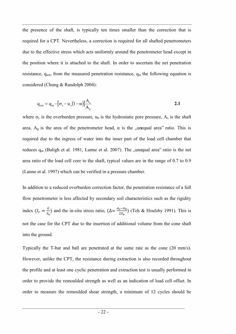
the position where it is attached to the shaft. In order to ascertain the net penetration
resistance, qnet, from the measured penetration resistance, qm the following equation is
considered (Chung & Randolph 2004):
p
sovmnet A
Aα1uσqq 2.1
where σv is the overburden pressure, u0 is the hydrostatic pore pressure, As is the shaft
area, Ap is the area of the penetrometer head, α is the „unequal area‟ ratio. This is
required due to the ingress of water into the inner part of the load cell chamber that
reduces qm (Baligh et al. 1981, Lunne et al. 2007). The „unequal area‟ ratio is the net
area ratio of the load cell core to the shaft, typical values are in the range of 0.7 to 0.9
(Lunne et al. 1997) which can be verified in a pressure chamber.
In addition to a reduced overburden correction factor, the penetration resistance of a full
flow penetrometer is less affected by secondary soil characteristics such as the rigidity
index
and the in-situ stress ratio,
(Teh & Houlsby 1991). This is
not the case for the CPT due to the insertion of additional volume from the cone shaft
into the ground.
Typically the T-bar and ball are penetrated at the same rate as the cone (20 mm/s).
However, unlike the CPT, the resistance during extraction is also recorded throughout
the profile and at least one cyclic penetration and extraction test is usually performed in
order to provide the remoulded strength as well as an indication of load cell offset. In
order to measure the remoulded shear strength, a minimum of 12 cycles should be

- 23 -
undertaken which is usually sufficient to achieve a steady remoulded soil resistance
(DeJong et al. 2010).
Figure 2.1. (a) T-bar; (b) Ball penetrometer
2.2.3.1. T-bar and ball penetrometer
The T-bar (Figure 2.1a) was first developed as a tool to improve the accuracy of
strength profiling in centrifuge tests in the University of Western Australia (Stewart &
Randolph 1991). The model T-bar comprises of a 5 mm diameter by 20 mm long
cylinder attached at right angles to the end of a vertical shaft. The penetrometer is
typically installed at a rate of 1 mm/s and the penetration resistance is measured with a
load cell that is housed within the shaft. The success of the tests led to field trials in
Australian waters described by Randolph et al. (1998). T-bars used in the field are

- 24 -
typically 250 mm in length with a 40 mm diameter. This gives a projected area of 10
times that of the standard cone shaft.
The ball penetrometer was first suggested as an alternative to the T-bar in order to
reduce the potential of axial bending of the shaft (Watson et al. 1998). Centrifuge
experiments on a 12 mm diameter model ball penetrometer were first described by
Watson et al. 1998 and the first field tests were carried out in 2003 as described in
Peuchen et al. (2005). The standard ball penetrometer used in field tests is 113 mm
diameter (area of 100 cm2) with a lightly sand blasted surface.
A recent development for the ball penetrometer has involved fitting pore pressure
sensors to obtain the coefficient of consolidation (Peuchen et al. 2005, Kelleher &
Randolph 2005). The „piezoball‟ ball penetrometer (Figure 1.1 and Figure 2.1b) shows
particular potential as being able to provide data on consolidation characteristics by
means of pore pressure dissipation tests (Low et al. 2007).
2.2.4. Interpretation of shear strength from full flow penetrometers
The main aim of this thesis is to analyse the undrained shear strength from static and
dynamic penetration in soil. The su profile can be determined from the net penetration
resistance (qT-bar or qball) of a deeply embedded T-bar or ball penetrometer using the
following expressions:
barT
barTu N
qs
2.2
ball
ballu N
qs 2.3
where NT-bar and Nball are the bearing capacity factors for a T-bar and ball penetrometer.
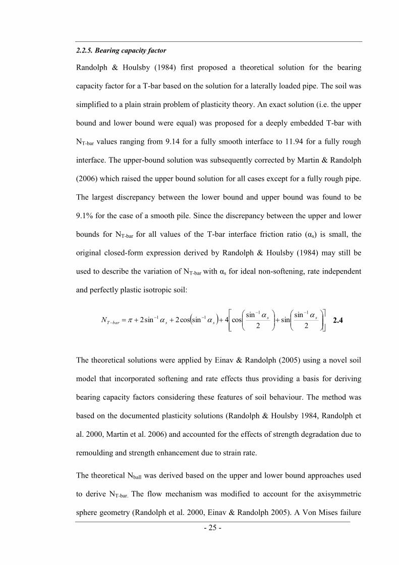
- 25 -
2.2.5. Bearing capacity factor
Randolph & Houlsby (1984) first proposed a theoretical solution for the bearing
capacity factor for a T-bar based on the solution for a laterally loaded pipe. The soil was
simplified to a plain strain problem of plasticity theory. An exact solution (i.e. the upper
bound and lower bound were equal) was proposed for a deeply embedded T-bar with
NT-bar values ranging from 9.14 for a fully smooth interface to 11.94 for a fully rough
interface. The upper-bound solution was subsequently corrected by Martin & Randolph
(2006) which raised the upper bound solution for all cases except for a fully rough pipe.
The largest discrepancy between the lower bound and upper bound was found to be
9.1% for the case of a smooth pile. Since the discrepancy between the upper and lower
bounds for NT-bar for all values of the T-bar interface friction ratio (αs) is small, the
original closed-form expression derived by Randolph & Houlsby (1984) may still be
used to describe the variation of NT-bar with αs for ideal non-softening, rate independent
and perfectly plastic isotropic soil:
2sin
sin2
sincos4sincos2sin2
1111 ss
ssbarTN
2.4
The theoretical solutions were applied by Einav & Randolph (2005) using a novel soil
model that incorporated softening and rate effects thus providing a basis for deriving
bearing capacity factors considering these features of soil behaviour. The method was
based on the documented plasticity solutions (Randolph & Houlsby 1984, Randolph et
al. 2000, Martin et al. 2006) and accounted for the effects of strength degradation due to
remoulding and strength enhancement due to strain rate.
The theoretical Nball was derived based on the upper and lower bound approaches used
to derive NT-bar. The flow mechanism was modified to account for the axisymmetric
sphere geometry (Randolph et al. 2000, Einav & Randolph 2005). A Von Mises failure

- 26 -
criterion was utilised to calculate the upper bound N and a Tresca model to calculate the
lower bound theoretical solution. The results range from 10.98 to 15.10 for a fully
smooth and fully rough ball respectively. These values are 20 to 28% (Tresca) or 18 to
21% (Von Mises) higher than the corresponding NT-bar. This method of analysis was
later improved by Zhou & Randolph (2009a) using large deformation finite element
(LDFE) analysis. The effects of strength degradation due to remoulding and strain rate
on NT-bar and Nball are expressed as:
idealbarTremrembarT NeNbarT
95
5.1
18.41
2.5
idealballremremball NeNball
95
5.1
18.41
2.6
where μ is the rate coefficient for a semi-logarithmic strain rate law, δrem is the ratio of
fully remoulded strength to intact soil strength and ξ95 is the accumulated absolute
plastic shear strain rate for the soil to undergo 95% remoulding. ξT-bar is taken as 3.7, ξball
is taken as 3.3. NT-bar(ideal) and Nball(ideal) are the NT-bar and the Nball for non-softening and
rate independent soil.
Equations 2.5 and 2.6 imply that the T-bar and sphere have the same average rate of
strain between the two flow mechanisms. A rate factor of 4.8 in both equations implies
that the average rate of strain experienced by soil flowing around either penetrometer is
some 104.8%/hr, i.e. five orders of magnitude greater than the reference strain of
1%/hour.
When equations 2.5 and 2.6 are considered with typical values of μ and ξ95, (0.05–0.2
and 10–25 respectively), the range of Nball (10–18) is approximately 20% higher than

- 27 -
the range of NT-bar (8–16). Similar results were found from analysing rate-independent
and non-softening soil (Lu et al. 2000) using LDFE analysis. However, this finding has
not been verified experimentally. In the centrifuge and field tests, the ratio has been
found to be almost identical (Chung & Randolph 2004, Boylan et al. 2007, Low et al.
2011, Colreavy et al. 2012). In fact, there is evidence suggesting lower rate dependency
for Nball compared to NT-bar. This may explain the disparity between theoretical and
experimental Nball/NT-bar which is a likely result of subtle soil characteristics such as soil
sensitivity and anisotropy that are not accounted for in the plasticity solution.
Another important finding from equations 2.5 and 2.6 is that NT-bar and Nball depend on
the sensitivity St (or the inverse of sensitivity, δrem, the remoulded shear strength ratio)
and the cumulative shear strain, δ95. This has been verified numerically and
experimentally by Yafrate & Dejong (2006) who found Nball and NT-bar values as low as
7 for high sensitivity soils.
In the field, a simpler approach is often adopted where a value of Nball and NT-deep = 10.5
is usually accepted (Stewart & Randolph 1991). This value has been established through
experimental calibration using a range of material types, stress histories and stress levels
(House et al. 2001). The solution takes into account that penetrometers used in the
centrifuge and in the field are neither fully smooth nor fully rough.
2.2.6. Interpretation of shear strength during shallow penetration
The su in the upper few meters of the seabed is a key parameter for the design of almost
all shallow offshore infrastructure such as, as-laid pipeline embedment (Westgate et al.
2012) and mobile seabed foundations (Feng et al. 2013). Assessing the shear strength
within the first 0.5 m soil depth (less than five diameters for a conventional 113 mm
diameter ball penetrometer) can be difficult with a T-bar or ball penetrometer. In order
- 28 -
to measure near surface strength (~1 kPa), shallow penetration effects must be
considered. Shallow penetration effects alter the usual relationship between the
penetration resistance (which is the measured quantity) and the soil strength (which is
the calculated quantity). The shallow penetration effects occur until the penetrometer
has become sufficiently embedded to reach the transition depth, which can take up to
several diameters embedment (see Section 2.2.6.1). This arises when a full-flow
mechanism around the penetrometer is established after the closure of soil above the top
of the penetrometer. In order to account for the changes, a number of factors must be
considered. These include an enhancement of the soil buoyancy (see Section 2.2.6.5), a
reduction of the bearing capacity factor (see Section 2.2.6.4) and a change to the
operative depth (see Section 2.2.6.6).
2.2.6.1. Transition depth
The transition depth or the limiting cavity depth has been estimated as the depth where
the soil flows over the top of the penetrometer, i.e. the crown of the T-bar or ball
penetrometer. Modern experiments have been carried out for a range of penetrometers
and subsea infrastructure such as T-bars and ball penetrometers (White et al. 2010,
Zhou et al. 2013) and also spudcans (Hossain et al. 2005).
2.2.6.2. Wall failure
Wall failure refers to cavity collapse; this is indicated by inward and downward soil
movements extending up to the soil surface. Skempton (1951) proposed a dimensionless
ratio of kd/sum (where sum is the mudline strength, k is the shear strength gradient and d
penetrometer diameter) in order to assess the stability of a circular footing. The stability
of a circular cavity has been investigated extensively by Meyerhof (1972) using
Rankine‟s pressure theory, and by Britto & Kusakabe (1982, 1983) using upper-bound
- 29 -
plasticity analysis. The cavity depth (Hw) at which wall failure is initiated is expressed
as:
su
wNsH 2.7
where γ' is the effective unit weight, su is the uniform undrained shear strength and Ns is
the stability number. Britto & Kusakabe (1983) formulated an empirical approach for Ns
for a circular footing. This approach, described in (SNAME, 1997), predicts the wall
failure or collapse of a cavity wall. However, with the availability of centrifuge
experiments, a different type of soil failure mechanism has been observed known as
flow failure.
2.2.6.3. Flow failure
Flow failure describes the progressive infilling of soil as it flows from beneath an object
to cover the top. At shallow penetration depths, flow failure is associated with upwards
and outwards soil flow resulting in heave at the soil surface. After reaching a certain
penetration depth, the soil flows back onto the exposed crown of the penetrometer.
During penetration, this gradual infilling continues until at some depth the penetrometer
reaches the transition depth where it becomes fully embedded. The result is a conical
crater that tapers towards the transition depth as shown in Figure 2.2 for a ball
penetrometer in uniform soil. This has been verified by both centrifuge observations
(Hossain et al. 2004b. Zhou et al. 2013) and field test subsea inspections (Kee & Ims
1984).
Centrifuge experiments have shown that the cavity depth due to flow failure is much
shallower than the criterion for wall failure (Hossain et al. 2005). A potential reason for
this is that circular cavity tested in the early studies was much smaller than the
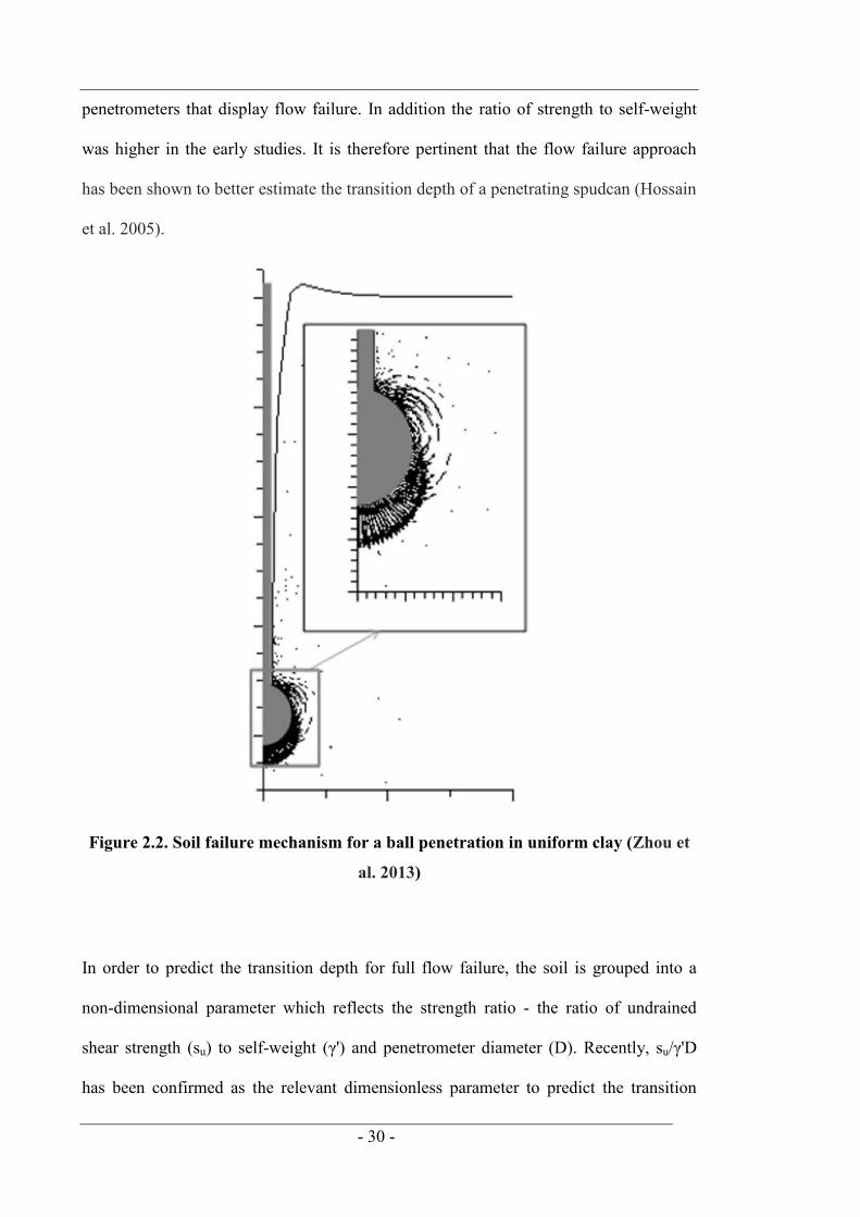
- 30 -
penetrometers that display flow failure. In addition the ratio of strength to self-weight
was higher in the early studies. It is therefore pertinent that the flow failure approach
has been shown to better estimate the transition depth of a penetrating spudcan (Hossain
et al. 2005).
Figure 2.2. Soil failure mechanism for a ball penetration in uniform clay (Zhou et
al. 2013)
In order to predict the transition depth for full flow failure, the soil is grouped into a
non-dimensional parameter which reflects the strength ratio - the ratio of undrained
shear strength (su) to self-weight (γ') and penetrometer diameter (D). Recently, su/γ'D
has been confirmed as the relevant dimensionless parameter to predict the transition
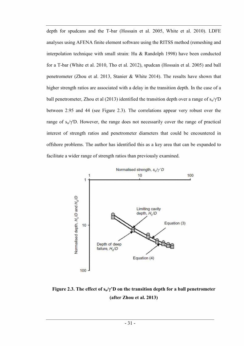
- 31 -
depth for spudcans and the T-bar (Hossain et al. 2005, White et al. 2010). LDFE
analyses using AFENA finite element software using the RITSS method (remeshing and
interpolation technique with small strain: Hu & Randolph 1998) have been conducted
for a T-bar (White et al. 2010, Tho et al. 2012), spudcan (Hossain et al. 2005) and ball
penetrometer (Zhou et al. 2013, Stanier & White 2014). The results have shown that
higher strength ratios are associated with a delay in the transition depth. In the case of a
ball penetrometer, Zhou et al (2013) identified the transition depth over a range of su/γ'D
between 2.95 and 44 (see Figure 2.3). The correlations appear very robust over the
range of su/γ'D. However, the range does not necessarily cover the range of practical
interest of strength ratios and penetrometer diameters that could be encountered in
offshore problems. The author has identified this as a key area that can be expanded to
facilitate a wider range of strength ratios than previously examined.
Figure 2.3. The effect of su/γ’D on the transition depth for a ball penetrometer
(after Zhou et al. 2013)
- 32 -
2.2.6.4. Bearing capacity factor variation with depth
Significant progress has been made in the theoretical studies of bearing capacity factors
for deeply embedded penetrometers. However, at shallow penetration depths a full-flow
mechanism does not develop around a penetrometer and su should be interpreted from
the measured penetration resistance using a shallow bearing capacity factor, Nb-shallow.
This is an important aspect of accurately quantifying the su over the upper 1 to 2 metres
of the seabed, if the shallow bearing capacity is ignored, the su may be underestimated
in the near surface soil (White et al. 2010).
Much of the available information on Nb-shallow comes from the study of shallow circular
foundations in non-homogeneous clay (e.g. Skempton 1951, Salencon & Matar 1982,
Houlsby & Wroth 1983, Kusakabe et al. 1986, Tani & Craig 1995, Martin & Randolph
2001). The Nb-shallow variation was first shown for a T-bar by White & Randolph (2007)
and result from LDFE and centrifuge analysis led to a shallow penetration framework
for a T-bar (White et al. 2010) and a ball penetrometer (Zhou et al. 2013). Both
frameworks derived a simple formula to quantify the variation of Nb-shallow with depth
which was conveniently defined as a proportion of the deep bearing factor, Nb-deep which
varies with the dimensionless strength ratio su/γ'D.
2.2.6.5. Soil buoyancy
Whilst a penetrometer is submerged in soil, the soil buoyancy increases the penetration
resistance. If soil heave at the mudline is ignored, Archimedes‟ principle can be used to
calculate the net upward force equal to the volume of the displaced soil multiplied by
the effective unit weight (γ') of the soil (Fbuoy = Vdispγ'). However, if there is a delay in
reaching the transition depth (which is the case for soils with a higher su/γ'D), there is an
extra component of soil buoyancy. This is caused by the cavity, which is formed by the
passage of the penetrometer. The soil that would have filled the cavity is instead

- 33 -
accommodated by heave at the soil surface. This increases the buoyancy contribution
because different degrees of soil heave, and thus work done against soil self-weight are
required at different depths. The heave effect has been captured for a T-bar and ball
penetrometer using a multiplier applied to the buoyancy force (Merifield et al. 2009,
White et al. 2010, Chatterjee et al. 2012, Zhou et al. 2013). The multiplier gradually
reduces to 1 when the penetrometer has reached the transition depth. For pipelines,
Merifield et al. (2009) suggested that the multiplier factor should be = 1.5. Chatterjee et
al. (2012) used LDFE analyses to show that it varies around ~ 1.5, depending on the
dimensionless shear strength gradient, kD/su,avg,whereas Zhou et al. (2013) estimated the
buoyancy factor as 3 for a ball penetrometer.
2.2.6.6. Operative depth
An important correction to the shallow penetration of a full flow penetrometer is to
account for the operative depth, (i.e. the depth at which the interpreted soil strength
applies). For a deeply embedded penetrometer with a symmetrical failure mechanism
above and below the penetrometer, qnet, and hence the inferred su, corresponds to the
mid-height of the penetrometer. This is highlighted in Figure 2.2 for a ball penetrometer
at the transition depth. For a shallowly embedded full-flow penetrometer, the
normalised operative depth, ŵop, is assumed to vary linearly from the invert to the mid-
height position which occurs at the transition depth (Hc) (White et al. 2010):
0.5DDH
0.5D
wc
op
www 2.8
where w is the invert depth and D is the penetrometer diameter.
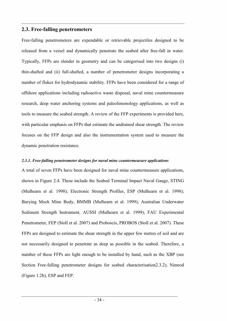
- 34 -
2.3. Free-falling penetrometers
Free-falling penetrometers are expendable or retrievable projectiles designed to be
released from a vessel and dynamically penetrate the seabed after free-fall in water.
Typically, FFPs are slender in geometry and can be categorised into two designs (i)
thin-shafted and (ii) full-shafted, a number of penetrometer designs incorporating a
number of flukes for hydrodynamic stability. FFPs have been considered for a range of
offshore applications including radioactive waste disposal, naval mine countermeasure
research, deep water anchoring systems and paleolimonology applications, as well as
tools to measure the seabed strength. A review of the FFP experiments is provided here,
with particular emphasis on FFPs that estimate the undrained shear strength. The review
focuses on the FFP design and also the instrumentation system used to measure the
dynamic penetration resistance.
2.3.1. Free-falling penetrometer designs for naval mine countermeasure applications
A total of seven FFPs have been designed for naval mine countermeasure applications,
shown in Figure 2.4. These include the Seabed Terminal Impact Naval Gauge, STING
(Mulhearn et al. 1998); Electronic Strength Profiler, ESP (Mulhearn et al. 1998);
Burying Mock Mine Body, BMMB (Mulhearn et al. 1999); Australian Underwater
Sediment Strength Instrument, AUSSI (Mulhearn et al. 1999); FAU Experimental
Penetrometer, FEP (Stoll et al. 2007) and Proboscis, PROBOS (Stoll et al. 2007). These
FFPs are designed to estimate the shear strength in the upper few metres of soil and are
not necessarily designed to penetrate as deep as possible in the seabed. Therefore, a
number of these FFPs are light enough to be installed by hand, such as the XBP (see
Section Free-falling penetrometer designs for seabed characterisation2.3.2), Nimrod
(Figure 1.2b), ESP and FEP.

- 35 -
In order to control the penetration resistance in different soil types, a number of FFPs
shown in Figure 2.4 are designed with interchangeable tip shapes and sizes (e.g. XDP,
AUSSI, FEP, PROBOS and STING) with most exhibiting flat or blunt ends (STING,
ESP, BBMB, AUSSI, FEP). Most FFP designs are full-shafted projectiles except the
STING (Figure 2.4b) which is a thin-shafted FFP with a 19 mm diameter shaft and a
tip-diameter in the range 25 - 70 mm (Abelev et al. 2009b). The merits of using a thin-
shafted FFP will be discussed in the following sections.
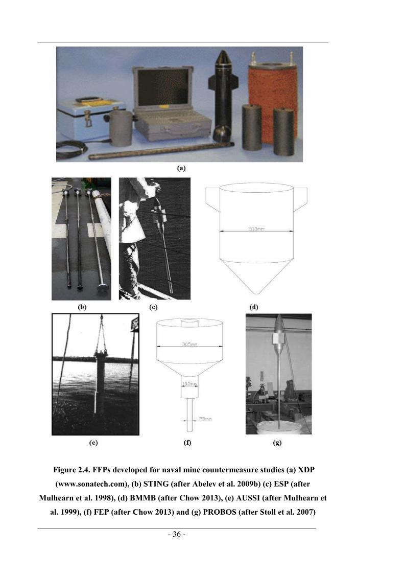
- 36 -
Figure 2.4. FFPs developed for naval mine countermeasure studies (a) XDP
(www.sonatech.com), (b) STING (after Abelev et al. 2009b) (c) ESP (after
Mulhearn et al. 1998), (d) BMMB (after Chow 2013), (e) AUSSI (after Mulhearn et
al. 1999), (f) FEP (after Chow 2013) and (g) PROBOS (after Stoll et al. 2007)
- 37 -
2.3.2. Free-falling penetrometer designs for seabed characterisation
A number of other FFPs have been developed for seabed characterisation (summarised
in Figure 2.5) including the Marine Impact Penetrometer (Dayal 1974); Marine
Sediment Penetrometer, MSP-1 and MSP-2 (Colp et al. 1975); free-fall penetrometer
(Denness et al. 1981); Expendable Bottom Probe, XBP (Akal & Stoll 1995); Free Fall
Cone Penetrometer, FFCPT (Mulukutla 2009); CPT lance (Stegmann 2007), Nimrod
(Stark et al. 2009a) and the CPT Stinger (Young et al. 2011, Jeanjean et al. 2012). These
FFPs are designed to penetrate as deeply as possible in the seabed. Therefore, they are
slender in geometry and often allow the inclusion of additional weights to increase the
penetration force (e.g. Marine Impact Penetrometer and LIRmeter). Most of the FFPs
shown in Figure 2.5 are full-shafted, conical-tipped penetrometers with shaft diameters
ranging from 36 to 70 mm and lengths ranging from 0.02 to 8.14 m.
- 38 -
Figure 2.5. FFP systems developed for applications in seabed characterisation (a)
Marine Impact Penetrometer (after Dayal et al. 1975), (b) MSP-2 (after Colp et al.
1975), (c) Freefall penetrometer (after Denness et al. 1981), (d) XBP (after Stoll &
Akal 1999), (e) FFCPT (www.brooke-ocean.com), (f) LIRmeter (after Stephan et
al. 2012), (g) CPT-Lance (after Stark et al. 2009b), (h) Nimrod (after Stark et al.
2009b), (i) CPT Stinger (after Young et al. 2011)

- 39 -
2.3.3. FFP measurement systems
FFPs measure the resistance force during penetration in soil in one of two ways, either
directly, using a load cell (or combination of load cells) (e.g. Steiner et al. 2012, Chow
et al. 2014) or indirectly, using an acoustic Doppler shift system or an accelerometer.
The indirect measurement technique calculates the resistance force by considering
Newton‟s second law of motion where the FFP is considered to be a single particle.
2.3.3.1. Acoustic Doppler system
The acoustic Doppler instrumentation system comprises a sound source mounted onto
the FFP and a receiving surface hydrophone on a support vessel. The frequency of the
signal received on the hydrophone is considered alongside the speed of sound in water
and soil to calculate the penetrometer velocity. The velocity data can be integrated to
provide an indirect calculation of penetration depth, thus allowing the vertically-
orientated motion response to be captured.
The Doppler measurement system is still in use today in the XDP which has been used
in over 270 individual deployments (e.g. Beard 1985, CYR 1990, Bowman et al. 1995,
Thompson et al. 2002, Ortman 2008) and results indicate that in the upper 2 m of soil,
the XDP provides reasonable assessment of undrained shear strength and penetration
depth (Beard 1981).
2.3.3.2. Accelerometer system
The majority of modern FFP designs (e.g. FFCPT, XBP, STING and AUSSI) are
instrumented with an internally-housed single-axis accelerometer that measures the
vertically-orientated acceleration during free-fall in water and dynamic penetration in
the seabed. The acceleration profile is numerically integrated in order to produce the
velocity profile which in turn is numerically integrated to produce the displacement
profile. The first accelerometers to be trialled in FFPs (e.g. Dayal 1974, Colp et al.
- 40 -
1975) and deep sea corers (Scott, 1970) were piezoelectric accelerometers. These
accelerometers rely on the use of a piezoelectric material as the sensing component
where the electrical output-signal is proportional to the stress applied to the
accelerometer. Piezoelectric accelerometers exhibit wide linear frequency ranges and
large amplitude ranges but struggle to accurately measure low frequency events. Early
FFP experiments using piezoelectric accelerometers reported some anomalous results
(e.g. Colp et al. 1975, Dayal 1974, Chari et al. 1978). These results are likely to occur
because during free-fall, a piezoelectric accelerometer loses signal as the piezoelectric
material discharges electrostatic charge (Stringer et al. 2010).
In a number a recent FFP experiments (Lavieri et al. 2011, Blake & O‟Loughlin 2015)
the piezoelectric accelerometer has been replaced with a MEMS accelerometer. MEMS
accelerometers have a number of advantages over piezoelectric accelerometers. For
example MEMS accelerometers can measure low frequency events and have
comparable performance during high frequency events (Stringer et al. 2010). Typical
acceleration profiles for a FFP test, measured with a MEMS accelerometer are shown in
Figure 2.6 and Figure 2.7. Figure 2.6 shows the measured acceleration alongside the
velocity and displacement profiles of a projectile during free-fall and dynamic
penetration in soil and Figure 2.7 highlights the parabolically-shaped acceleration
profile after the FFP has impacted the seabed.

- 41 -
Figure 2.6. Typical velocity and penetration depth with time profiles for the FFP
instrumented with an accelerometer (Chow & Airey 2010b)
Figure 2.7. Acceleration profile in soil (after Stephan et al. 2012)
2.3.4. Experimental and field studies on free-falling penetrometers
As shown in Figure 2.4 and Figure 2.5 a relatively large number of FFP designs have
been tested at full-scale. Some of the FFPs including the XDP, XBP, STING, FFCPT,
CPT-Lance and Nimrod have been widely investigated in multiple locations. For
example, the XDP, (shown in Figure 2.4a) has been extensively tested in over 270 field
tests (Beard 1977, 1981, 1985, Bowman et al. 1995, Douglas & Wapner 1996,
Thompson et al. 2002, Ortman 2008) and the XBP (Figure 2.5d) has been tested in over

- 42 -
500 field tests in various locations such as New York Harbour, Italy, Spain, Germany,
Turkey and in the Black Sea and the Gulf of Mexico (Stoll & Akal 1999).
Results from full-scale field trials suggest that the final embedment depth of a FFP is
found to depend on its mass, soil type, penetration velocity and geometry. For example
the XDP reported by Bowman et al (1995) weighed approximately 0.26 kN and
achieved tip embedments between 0.5–3 m. Whereas the XDP used by Beard (1977,
1981, 1985) was longer and weighed approximately 1.31 kN and reported larger tip
embedments in the range 5.8–10 m.
In addition to mass, the final embedment depth of a FFP is heavily dependent on soil
type with reduced embedment depths being observed in sandy soil compared to soft
clay. For example, very low tip-embedment of less than 0.75 m has been reported from
experiments carried out on the ESP (Figure 2.10) which comprised 32 tests in carbonate
sands and muds. Similar results have been reported using the AUSSI (Mulhearn et al.
1999), BBMB (Mulhearn et al. 1999), ESP (Mulhearn et al. 1998) and STING
(Mulhearn et al. 1999) where very low tip-embedment in the range of 0.22 to 1 m were
achieved in hard/shelly sand in Sydney harbour. Stark et al (2009b, 2012) also reported
very low tip-embedment in the range 0.04 to 0.34 m in North Sea quartz sand and also
carbonate sand in Hawaii. At the same test sites, the CPT-Lance (Figure 2.5g) achieved
very low tip-embedment between 0.08 to 0.12 m (Stark et al. 2009b) whereas much
higher tip-embedment of approximately 5 to 6 m was reported in Osthafen silty mud
(Stegmann 2007) and Holocene silty clay (Steiner et al. 2012). Laboratory experiments
carried out on the Marine Impact Penetometer (Dayal 1974, Dayal et al. 1975), XBP
(Akal & Stoll 1995) and PROBOS (Stoll et al. 2007) in sand revealed similar results
where the low tip-embedment was due to the effects of dilative behaviour. This infers
that the application of FFPs may be restricted to soft soils such as clays and silts.
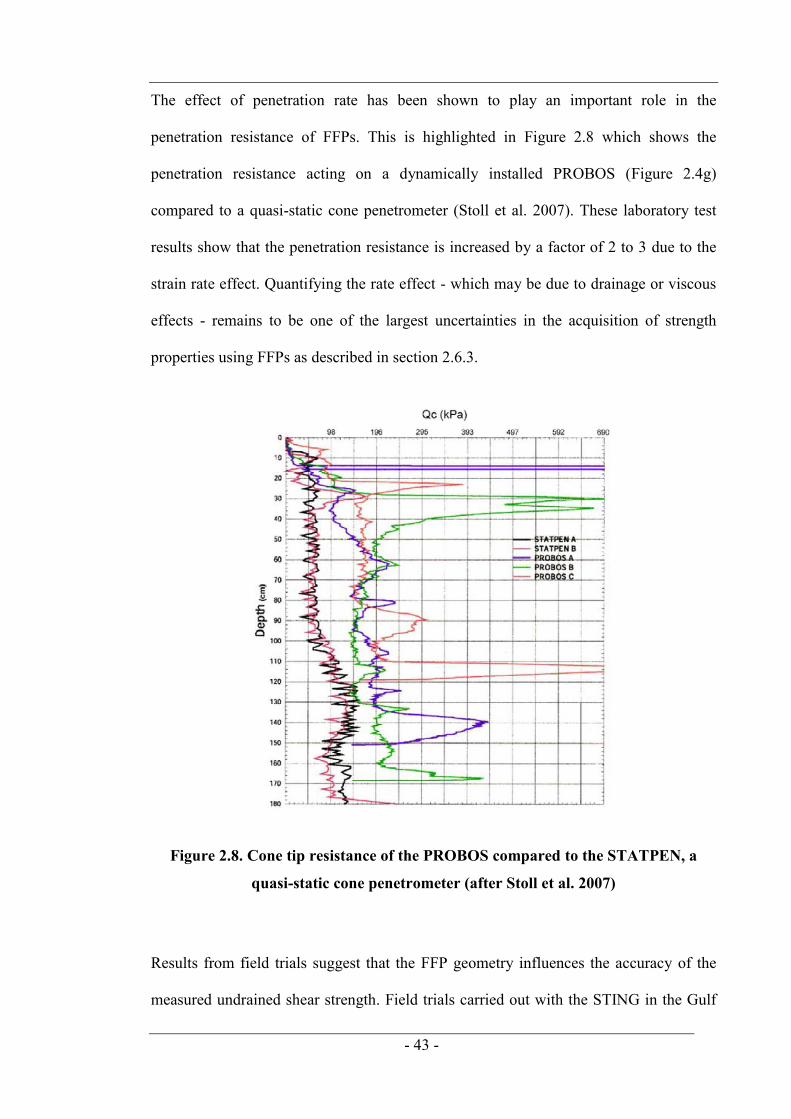
- 43 -
The effect of penetration rate has been shown to play an important role in the
penetration resistance of FFPs. This is highlighted in Figure 2.8 which shows the
penetration resistance acting on a dynamically installed PROBOS (Figure 2.4g)
compared to a quasi-static cone penetrometer (Stoll et al. 2007). These laboratory test
results show that the penetration resistance is increased by a factor of 2 to 3 due to the
strain rate effect. Quantifying the rate effect - which may be due to drainage or viscous
effects - remains to be one of the largest uncertainties in the acquisition of strength
properties using FFPs as described in section 2.6.3.
Figure 2.8. Cone tip resistance of the PROBOS compared to the STATPEN, a
quasi-static cone penetrometer (after Stoll et al. 2007)
Results from field trials suggest that the FFP geometry influences the accuracy of the
measured undrained shear strength. Field trials carried out with the STING in the Gulf
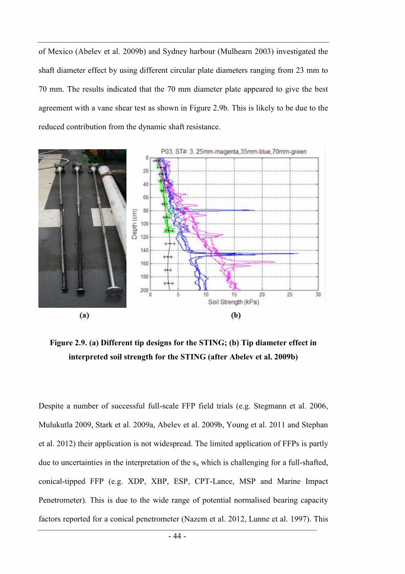
- 44 -
of Mexico (Abelev et al. 2009b) and Sydney harbour (Mulhearn 2003) investigated the
shaft diameter effect by using different circular plate diameters ranging from 23 mm to
70 mm. The results indicated that the 70 mm diameter plate appeared to give the best
agreement with a vane shear test as shown in Figure 2.9b. This is likely to be due to the
reduced contribution from the dynamic shaft resistance.
Figure 2.9. (a) Different tip designs for the STING; (b) Tip diameter effect in
interpreted soil strength for the STING (after Abelev et al. 2009b)
Despite a number of successful full-scale FFP field trials (e.g. Stegmann et al. 2006,
Mulukutla 2009, Stark et al. 2009a, Abelev et al. 2009b, Young et al. 2011 and Stephan
et al. 2012) their application is not widespread. The limited application of FFPs is partly
due to uncertainties in the interpretation of the su which is challenging for a full-shafted,
conical-tipped FFP (e.g. XDP, XBP, ESP, CPT-Lance, MSP and Marine Impact
Penetrometer). This is due to the wide range of potential normalised bearing capacity
factors reported for a conical penetrometer (Nazem et al. 2012, Lunne et al. 1997). This
- 45 -
problem is somewhat reduced when a thin-shafted FFP (e.g. STING) is considered.
Although not as well investigated as a full-shafted FFP, the thin-shafted FFP seem to
provide a better assessment of the undrained shear strength due to the negligible
dynamic shaft resistance (Mulhearn 2003). This reduces the complexity of the data
interpretation, and avoids the difficulties caused by the shaft resistance which appears to
attract greater rate effects than the tip resistance (Dayal et al. 1975, Steiner et al. 2014).
In addition, a thin-shafted geometry is similar to the full-flow penetrometers (described
in Section 2.2.3), where a narrow band of bearing capacity factors have been derived
from plasticity theory (see Section 2.2.5).
2.4. Oceanic waste carriers
Research on the dynamic penetration of streamlined projectiles into the seabed
commenced in the 1960s in order to assess the feasibility of using FFPs as oceanic
waste carriers for the disposal of radioactive material. Field experiments trialled a
number of projectiles at two sites in the Atlantic Ocean, the Great Meteor East (GME)
(Freeman et al. 1984, Freeman et al 1988) and the Nares Abyssal Plain (NAP) (Freeman
& Burdett 1986). The first tests was carried out using four similar penetrometer designs
including the European Standard Penetrometer, shown in Figure 2.10, which measured
3.25 m long, 0.325 m diameter and weighed 1.8 tons in air (Freeman et al. 1984). The
European Standard Penetrometer was subsequently adopted as the standard for
comparison with later experiments at the NAP site. Results indicated that impact
velocities of 30 to 35 m/s were achieved, resulting in embedment of up to 46 to 51 m at
the GME site. At the NAP site, impact velocities between 45 to 56 m/s were achieved,
resulting in penetration depths of 21 to 35 m. Separate field tests relating to the disposal
of nuclear waste were also carried out in Antibes in the Mediterranean Sea. A total of
nine tests were conducted with five different penetrometer designs resulting in

- 46 -
penetration depths in the range of 9 to 15 m (Audibert et al. 2006). The reduced
embedment depth was reported to be due to much stiffer soil in the Mediterranean site
compared to the GME and NAP sites.
Figure 2.10. The European Standard Penetrometer (Freeman & Burdett, 1986)
2.5. Dynamically installed anchors
Four types of dynamically installed anchor (Figure 2.11) have been developed: the Deep
Penetrating Anchor (DPA) (Lieng et al. 1999), the Torpedo Anchor (Medeiros. 2002),
the OMNI-Max anchor (Zimmerman & Spikula 2005) and the Deep Embedded Plate
Anchor (DEPLA) (Blake et al. 2012). These anchors have mainly been developed in an
effort to provide floating production platforms with a cost effective anchoring solution.
The DPA and Torpedo anchor are similar in function insofar as they are designed to
deeply-penetrate the seabed, typically up to 3 times the anchor length (O'Loughlin et al.
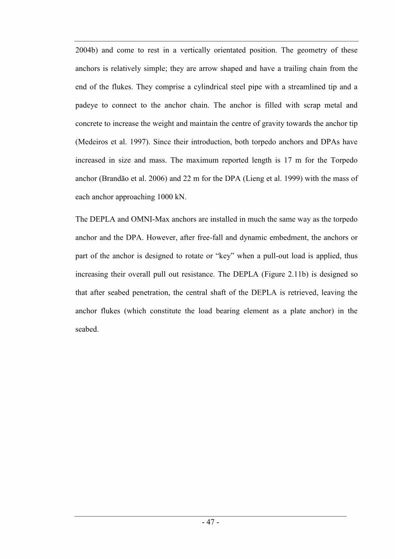
- 47 -
2004b) and come to rest in a vertically orientated position. The geometry of these
anchors is relatively simple; they are arrow shaped and have a trailing chain from the
end of the flukes. They comprise a cylindrical steel pipe with a streamlined tip and a
padeye to connect to the anchor chain. The anchor is filled with scrap metal and
concrete to increase the weight and maintain the centre of gravity towards the anchor tip
(Medeiros et al. 1997). Since their introduction, both torpedo anchors and DPAs have
increased in size and mass. The maximum reported length is 17 m for the Torpedo
anchor (Brandão et al. 2006) and 22 m for the DPA (Lieng et al. 1999) with the mass of
each anchor approaching 1000 kN.
The DEPLA and OMNI-Max anchors are installed in much the same way as the torpedo
anchor and the DPA. However, after free-fall and dynamic embedment, the anchors or
part of the anchor is designed to rotate or “key” when a pull-out load is applied, thus
increasing their overall pull out resistance. The DEPLA (Figure 2.11b) is designed so
that after seabed penetration, the central shaft of the DEPLA is retrieved, leaving the
anchor flukes (which constitute the load bearing element as a plate anchor) in the
seabed.

- 48 -
Figure 2.11. Dynamically installed anchors (Medeiros, 2002); (b) Torpedo Anchor
(Brandão et al. 2006)
2.5.1. Experimental and field studies on dynamically installed anchors
The Torpedo anchor has seen widespread commercial use in Brazilian waters since the
late 1990s. Medeiros (2002) reported the first commercial application of torpedo
anchors for anchoring flexible risers in the Campos Basin, Brazil in water depths of up
to 1000m. Since then, over 1000 torpedo anchors have been installed in offshore Brazil
for the mooring of flexible risers, MODUs and FPSOs (Wilde 2009).
- 49 -
The DPA (Figure 2.11a) was first introduced by (Lieng et al. 1999) as an alternative to
the Torpedo anchor. Although the anchor is not in wide use today, a number of reduced-
scale and full-scale tests have been carried out (Strum et al. 2011, Lieng et al 2010). The
installation of a DPA is achieved by lowering the anchor from a stationary vessel to a
target height (typically 40–50 m above the seabed). In spring 2003, twelve 1–3 scale, 4
m long DPA models were tested in both the Trondheim Fjord and at the Troll Field in
the North Sea. In these experiments, at least one anchor was instrumented with a depth
sensor, accelerometer, inclinometer, and pore pressure sensors. However, the results of
these tests have not been published.
In 2008, a total of twelve 1:3 reduced-scale model DPAs were tested in the Troll Field
in the North Sea. An important finding from the 1:3 scale tests was that the
hydrodynamic stability was verified. During free-fall, very little lateral drift was
recorded and on average a 2° tilt was observed for tests released from 15 m to 75 m
above the mudline which embedded between 7 and 9 m (Strum et al. 2011). In 2009,
two full-scale DPAs were installed on StatoilHydro's Gjøa field in 360 meters of water.
The anchors were 13 m in length and had a mass of 736 kN. The DPAs were dropped
from heights of 50 m and 75 m and achieved impact velocities of 24.5 and 27 m/s,
corresponding to tip-embedment of 24 m and 31 m respectively (Lieng et al. 2010).
Full scale tests of the OMNI-Max anchor have been conducted in over 1600 m of water
in the Gulf of Mexico (Shelton, 2007) in soft to medium clay using a 9 m long anchor
with a mass of 333 kN (Zimmerman, 2007). The tests demonstrated the stability of the
anchor during free-fall. In addition, the same anchor design has been used for the
mooring of MODUs in the Gulf of Mexico in 427 m water depth (Shelton, 2011).
- 50 -
A number of field tests using reduced-scale DEPLAs have been reported by (Blake &
O‟Loughlin 2012, 2015, Blake et al. 2014). The tests demonstrated that the tip
embedment was similar to other dynamically installed anchors and was in the range 2–
3.7 times the anchor length. However, the studies reported far higher pull-out capacity
compared to the Torpedo anchor and DPA due to the large projected area of the rotated
flukes in the seabed.
2.5.2. Centrifuge experiments
Centrifuge experiments are often used in the analysis of dynamically installed anchors
partly because high prototype velocities up to 25 m/s cannot be achieved with reduced
scale models at 1 g. Centrifuge experiments have been carried out on reduced-scale
1:200 model DPAs (Figure 2.11a, Richardson 2008, O‟Loughlin et al. 2009), Torpedo
anchors (Figure 2.11d, Hossain et al. 2014), OMNI-Max (Figure 2.11c, Gaudin et al
2013) and DEPLA (Figure 2.11b, O‟Loughlin et al. 2014).
The results are similar to the FFP field test results where the final embedment depth is
dependent on soil type. The experiments carried out in normally consolidated kaolin
clay typically embedded between 2.0–2.9 times the anchor length (O‟Loughlin et al.
2009, (O‟Loughlin et al. 2014) and in slightly overconsolidated kaolin clay the anchors
typically embedded between 1.2–2.1 (Hossain et al. 2014) and 1.8–2 (Gaudin et al
2013). However, the experiments carried out in stiffer calcareous silt revealed far lower
embedment depths in the range 1.14–1.46 (Gaudin et al. 2013) and approximately 1.17–
1.4 (Hossain et al. 2014).
- 51 -
2.6. Resistance forces acting on a projectile during dynamic
embedment in soil
The resistance forces acting on a deeply-embedded full-shafted FFP (with a 60° conical
tip, similar in geometry to most FFPs (e.g. Stegmann et al. 2006, Mosher et al. 2007,
Stark et al. 2009, Young et al. 2011, Stephan et al. 2012) and a thin-shafted FFP (similar
in geometry to the STING with a cylindrical tip, see Figure 2.4b) are shown in Figure
2.12a and Figure 2.12b. The net resistance force of each FFP comprises the drag force
(Section 2.6.1), the bearing force (Section 2.6.6) and for the case of the full-shafted
FFP, the side friction force (Section 2.6.6). Additional resistance forces (not shown on
Figure 2.12a and Figure 2.12b) that have been considered in the analysis of FFPs
include the added mass (Section 2.6.2) and the strain rate-enhanced soil resistance
(Section 2.6.3.1).

- 52 -
Figure 2.12. (a) Forces acting on a full-shafted penetrometer and (b) Thin-shafted
penetrometer during installation
2.6.1. Fluid drag
The fluid drag or drag refers to the resistance force that a moving object is subjected to
in a fluid. The total drag is the sum of two components: (i) form drag, also commonly
known as pressure drag, caused by an adverse pressure gradient between the front and
rear of the object which creates an opposing force and (ii) friction drag, also referred to
as viscous drag. The friction drag is dominant during very low flow rates, however, for
most practicable cases, the contribution of the friction drag to the total drag is usually
- 53 -
low ~ 2–3% for bluff bodies such as a cylinder or a sphere (Achenbach 1971). The drag
force is expressed as (Morison et al. 1950):
2
21 AvCF Dd 2.9
where ρ is the fluid density, A is the area and v is the velocity. CD is the drag
coefficient, dictated largely by object geometry, i.e. the ratio of body length over
diameter, surface roughness and Reynolds Number (Pazwash & Robertson 1975).
2.6.1.1. Drag in water
In classical fluid mechanics studies of Newtonian fluids (e.g. air and water), the shear
stress is linearly proportional to the shear strain rate and the Reynolds Number, Re is
defined as the ratio of the inertia forces to the viscous forces, expressed as:
vDRe 2.10
Where D, is the projectile diameter, and is the temperature and salinity-dependent
kinematic viscosity of the fluid,
where, ɳ is the absolute viscosity.
For FFPs, it is commonly assumed that the CD is the same in both water and soil
regardless of any difference on Re with reported values ranging widely from 0.2–1.2
(True 1976, Freeman et al. 1984, Freeman & Burdet 1986, Bowman et al. 1995, Øye
2000, Cenac II 2011, Hansaloo et al. 2012).
However, for a simplified geometry such as a sphere, the experimental correlation for
CD versus Re has been investigated extensively for Re < 2 x 10⁵. A non-exhaustive list
of the experimental data includes: (Allen 1900, Shakespear 1914, Wieselsberger, 1923,

- 54 -
Bacon & Reid 1924, Liebster 1927, Lunnon 1928, Schmiedel 1928, Millikan & Klein
1933, Moller 1938, Davies 1945, Pettyjohn & Christiansen 1948, Gunn & Kinzer 1949,
Maxworthy 1965, 1969, Goin & Lawrence 1968, Pruppacher & Steinberger 1968,
Dennis & Walker 1971, Roos & Willmarth 1971, Achenbach 1972, Hartman et al.
1994, Beard & Pruppacher 1969, Rimon & Cheng 1969). The correlation for CD and Re
agree well with theoretically derived parameters for various Re ranges. For example, for
Re < 0.5 the correlation agree with theoretical values derived by Stokes (1880) and for
all ranges if Re, the correlation agree with theoretical values derived using a
computational fluid dynamics (CFD) (e.g. Richardson. 2008, Jones & Clarke 2008).
Figure 2.13. Drag coefficient for uniform flow past a sphere R = Re < 2 x 10⁵ (480
data points) after (Brown & Lawler 2003)
For a sphere in the laminar flow regime, Re << 1 no separation between the fluid and
sphere exists and the friction drag dominates, resulting in very high CD. With increasing
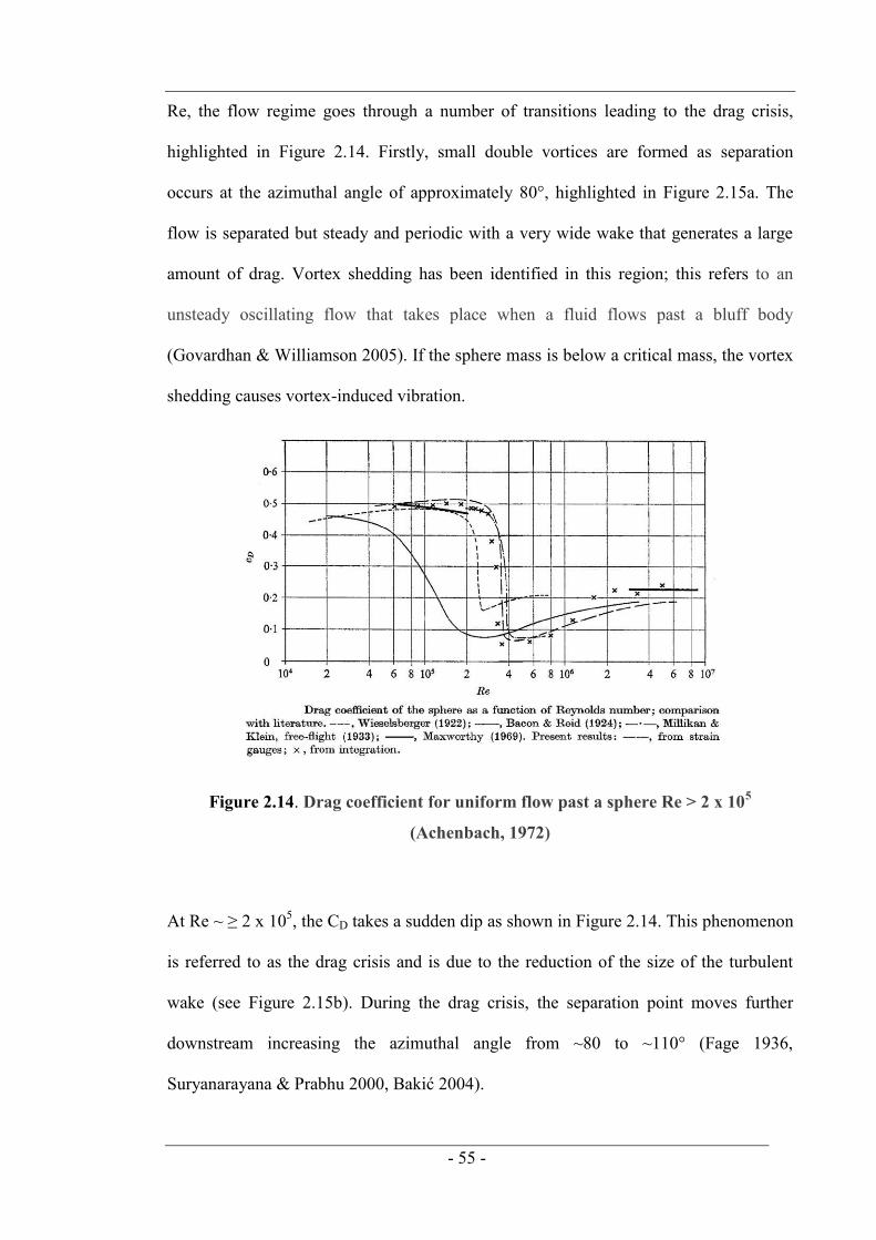
- 55 -
Re, the flow regime goes through a number of transitions leading to the drag crisis,
highlighted in Figure 2.14. Firstly, small double vortices are formed as separation
occurs at the azimuthal angle of approximately 80°, highlighted in Figure 2.15a. The
flow is separated but steady and periodic with a very wide wake that generates a large
amount of drag. Vortex shedding has been identified in this region; this refers to an
unsteady oscillating flow that takes place when a fluid flows past a bluff body
(Govardhan & Williamson 2005). If the sphere mass is below a critical mass, the vortex
shedding causes vortex-induced vibration.
Figure 2.14. Drag coefficient for uniform flow past a sphere Re > 2 x 10⁵
(Achenbach, 1972)
At Re ~ ≥ 2 x 10⁵, the CD takes a sudden dip as shown in Figure 2.14. This phenomenon
is referred to as the drag crisis and is due to the reduction of the size of the turbulent
wake (see Figure 2.15b). During the drag crisis, the separation point moves further
downstream increasing the azimuthal angle from ~80 to ~110° (Fage 1936,
Suryanarayana & Prabhu 2000, Bakić 2004).

- 56 -
Figure 2.15. Laminar-separated flow and turbulent flow over a sphere - (after
Finnemore & Franzini 2001)
2.6.1.2. Drag in soil
Compared to the large amount of research on Newtonian fluids, very little is known
about the drag forces during flow through soil. However, most geotechnical studies on
FFPs have considered the drag force in soil in view of the very soft viscous soil that is
often encountered at the surface of most seabed deposits (e.g. True 1976, Bowman et al.
1995, Mulhearn et al. 1998, Fernandes et al 2006, Abelev et al. 2009b, O‟Loughlin et al.
2009). In these studies it is commonly assumed that the drag coefficient is the same in
both soil and water. A small number of fluid mechanics experimental studies have been
carried out in non-Newtonian fluid such as debris flow material (Coussot et al. 1998)
and clay-water mixtures, similar to the upper layer of an offshore seabed (e.g. Houwink,
1952, Pazwash & Robertson 1969, Robertson & Pazwash 1971). The results indicate
that these fluids exhibit non-Newtonian behaviour, formulated in terms of Herschel-
Bulkley model which accounts for the effect of strain rate using an additive term:
- 57 -
ny 2.11
where τ is the shear stress, η is a measure of viscosity and, is the yield stress or the
minimum shear stress required to initiate flow at a particular strain rate, and n is the
shear-thinning (pseudoplastic) index.
Within the fluid mechanics framework, the drag force is estimated using Equation 2.9,
and the CD has been proposed to be a function of the non-Newtonian Reynolds number,
Renon-Newtonian where,
2
Re vNewtoniannon
2.12
where ρ is the density, v is velocity and τ is the mobilised shear stress within the flow
material (Equation 2.11). Research on the rheology of debris flow materials, such as an
underwater landslide on a submerged pipeline has been carried out and an empirical
correlation has been proposed (Zakeri et al. 2008, Zakeri et al. 2009):
25.1Re5.174.1
NewtoniannonDC
2.13
2.6.2. Hydrodynamic mass force
In the case of non-stable flows where the object is accelerating or decelerating, there is
an additional force opposing motion called the hydrodynamic mass force. This force is
required because some volume of fluid (V) surrounding an object is accelerated from
rest to a velocity capable of displacing the fluid out of its path as the object and fluid
cannot occupy the same physical space simultaneously (Sumer & Fredsoe 1997). The
- 58 -
force is manifested as inertia or added mass, m' that is added to the mass of the system
where m' can be calculated in the traditional way (Lamb 1932):
VCm m 2.14
Where Cm is the geometry dependent hydrodynamic-mass coefficient of a sphere that
has been shown both experimentally and theoretically to be equal to 0.5, ρ is the density
of the fluid and V is the enclosed volume of the accelerated body.
2.6.3. Strain rate effects in clay
The geotechnical resistance forces acting on the FFPs shown in Figure 2.12 (i.e. the
bearing and shaft resistance) are linked to the undrained shear strength which is
considered to be a function of strain rate. This has been backed up with a large database
of plates, cones and full-flow penetrometer tests in clays (e.g. Murff & Coyle 1973,
Lehane et al. 2009). Figure 2.16 plots the normalised penetration resistance and the
normalised velocity (V = vD/ch) where v is the penetration velocity, D in the diameter
and ch is the horizontal coefficient of consolidation. Below a V of ~ 15, consolidation is
dominant and viscous effects are almost negligible (Lehane et al. 2009).
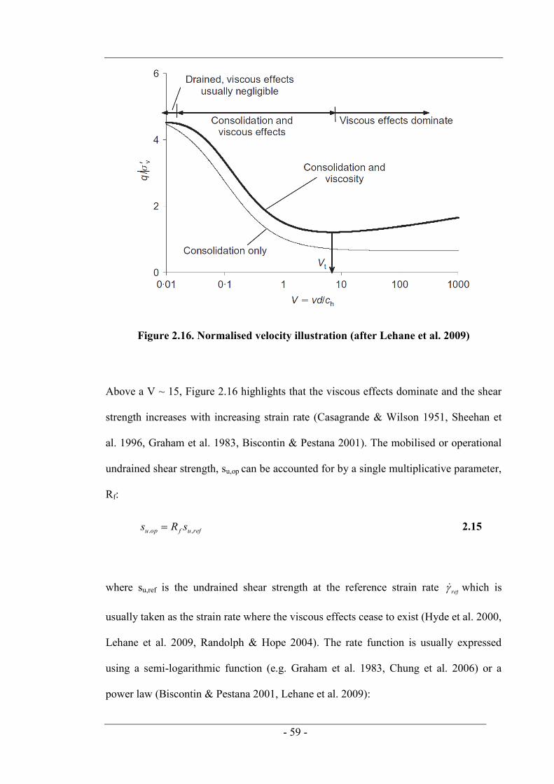
- 59 -
Figure 2.16. Normalised velocity illustration (after Lehane et al. 2009)
Above a V ~ 15, Figure 2.16 highlights that the viscous effects dominate and the shear
strength increases with increasing strain rate (Casagrande & Wilson 1951, Sheehan et
al. 1996, Graham et al. 1983, Biscontin & Pestana 2001). The mobilised or operational
undrained shear strength, su,op can be accounted for by a single multiplicative parameter,
Rf:
refufopu sRs ,. 2.15
where su,ref is the undrained shear strength at the reference strain rate ref which is
usually taken as the strain rate where the viscous effects cease to exist (Hyde et al. 2000,
Lehane et al. 2009, Randolph & Hope 2004). The rate function is usually expressed
using a semi-logarithmic function (e.g. Graham et al. 1983, Chung et al. 2006) or a
power law (Biscontin & Pestana 2001, Lehane et al. 2009):
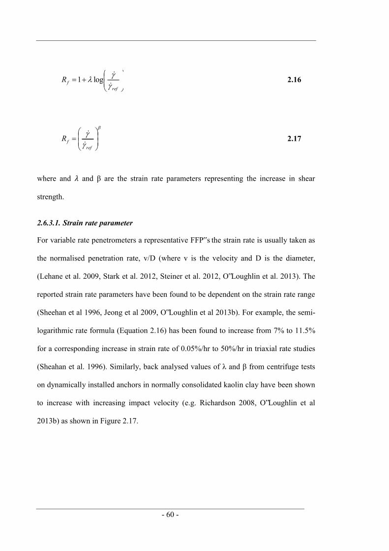
- 60 -
reffR
log1 2.16
reffR
2.17
where and and β are the strain rate parameters representing the increase in shear
strength.
2.6.3.1. Strain rate parameter
For variable rate penetrometers a representative FFP‟s the strain rate is usually taken as
the normalised penetration rate, v/D (where v is the velocity and D is the diameter,
(Lehane et al. 2009, Stark et al. 2012, Steiner et al. 2012, O‟Loughlin et al. 2013). The
reported strain rate parameters have been found to be dependent on the strain rate range
(Sheehan et al 1996, Jeong et al 2009, O‟Loughlin et al 2013b). For example, the semi-
logarithmic rate formula (Equation 2.16) has been found to increase from 7% to 11.5%
for a corresponding increase in strain rate of 0.05%/hr to 50%/hr in triaxial rate studies
(Sheahan et al. 1996). Similarly, back analysed values of λ and β from centrifuge tests
on dynamically installed anchors in normally consolidated kaolin clay have been shown
to increase with increasing impact velocity (e.g. Richardson 2008, O‟Loughlin et al
2013b) as shown in Figure 2.17.
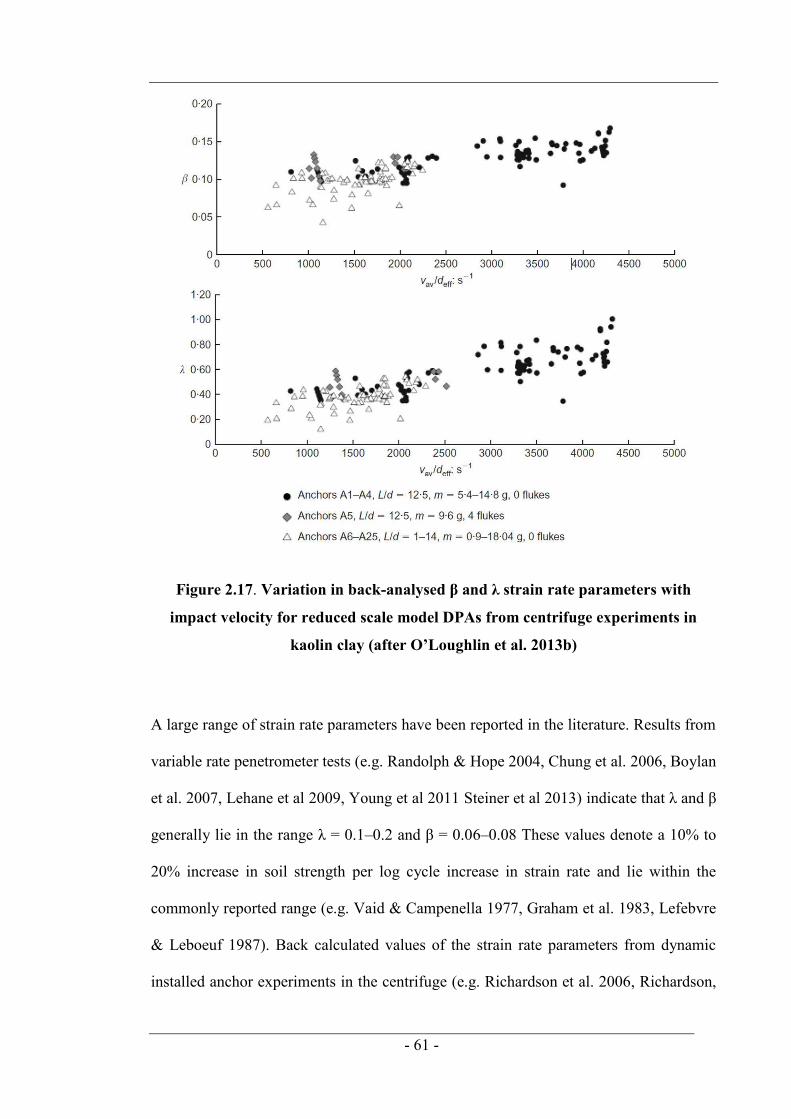
- 61 -
Figure 2.17. Variation in back-analysed β and λ strain rate parameters with
impact velocity for reduced scale model DPAs from centrifuge experiments in
kaolin clay (after O’Loughlin et al. 2013b)
A large range of strain rate parameters have been reported in the literature. Results from
variable rate penetrometer tests (e.g. Randolph & Hope 2004, Chung et al. 2006, Boylan
et al. 2007, Lehane et al 2009, Young et al 2011 Steiner et al 2013) indicate that λ and β
generally lie in the range λ = 0.1–0.2 and β = 0.06–0.08 These values denote a 10% to
20% increase in soil strength per log cycle increase in strain rate and lie within the
commonly reported range (e.g. Vaid & Campenella 1977, Graham et al. 1983, Lefebvre
& Leboeuf 1987). Back calculated values of the strain rate parameters from dynamic
installed anchor experiments in the centrifuge (e.g. Richardson et al. 2006, Richardson,

- 62 -
2008, O‟Loughlin et al. 2009) report higher values for λ and β that lie in the range λ =
0.19–1 and β = 0.06–0.17. The wide range of λ and β values may be (at least in part)
attributed to the order of magnitude difference between the strain rate, and the
reference strain rate, ref . The maximum (which is proportional to v/D) associated
with the free-falling experiments in the centrifuge can be as high as 4250 s-1 (see Figure
2.17) or five to seven orders of magnitude greater than ref for a standard penetration
rate of 0.2 s-1 and up to 10 orders of magnitude greater than the nominal strain rate
associated with laboratory triaxial compression tests and shear vane tests which lie in
the range 3 x 10⁻⁶ to 2 x 10⁻³ s-1 (Einav & Randolph 2006). Therefore it is difficult to
deduce strain rate parameters from laboratory analysis to be adopted in free-fall
experiments in the centrifuge or the field. Similarly, caution is advised when comparing
the strain rates in the centrifuge to the field tests. The strain rates (proportional to v/D)
in the centrifuge are higher because the impact velocities are similar but the diameter is
reduced due to the scaling factor.
2.6.3.2. Dependency of rate parameters on penetrometer geometry
The effects of strain rate dependency on full-flow penetrometer geometry have been
investigated numerically and experimentally. Higher rate parameters have been obtained
for a ball penetrometer than a T-bar (Einav & Randolph 2006, Zhou & Randolph 2007,
Lehane et al. 2009). However, these results were not verified experimentally by Chung
& Randolph (2004). Similarly, for the thin-shafted STING (Figure 2.4b) negligible tip
shape effects were found on the rate dependence (Hurst & Murdoch 1991, Mulhearn
2003).
For full-shafted FFP tests, higher rate dependency has been reported for the shaft
resistance compared to tip resistance (Dayal et al. 1975, Steiner et al. 2014, Chow et al

- 63 -
2014). The higher dependency is believed to be due to the pattern of shearing which is
concentrated in shear bands, and has been accounted for by enhancing the power strain
rate law (Equation 2.17) using a multiplicative term (Zhu & Randolph 2011, Einav &
Randolph 2006). The rate dependency of the shaft is approximately 19–23% higher than
the tip (Chow et al 2014).
2.6.3.3. Dependency of rate parameters on material properties
A large number of soil properties including plasticity, moisture content, stress history,
anisotropy and soil sensitivity has been found to influence strain rate dependency. Soil
plasticity has been recognised to influence the strain rate effect since the 1960s. Higher
rate effects have been observed with higher soil plasticity from triaxial tests (e.g.
Gibson & Coyle 1968, Nakase & Kamei 1986, Diaz-Rodriguez & Martinez-Vasquez
2005) as well as vane studies (e.g. Bjerrum 1973, Peuchen & Mayne 2007, Schlue et al.
2010). Mixed results have been reported on the soil moisture content with most
experiments showing that a reduced moisture content results in lower strain rate effects
(e.g. Gibson & Coyle 1968, Dayal 1974, Brown & Hyde 2008b, Abelev & Valent 2009,
Schlue et al. 2010). However, contradictory results were observed in soils with high
moisture contents, above the liquid limit (LL) from submarine landslide studies (Jeong
et al. 2009) and from vane, viscometer, T-bar and ball penetrometer studies in kaolin
clay (Boukpeti et al. 2012). Therefore, the rate dependency on moisture content or soil
strength may be restricted to soils with moisture contents lower than the liquid limit.
Stress history has been investigated by Lehane et al. (2009) through penetration tests
into soil with an over consolidation ratio (OCR) of 1, 2 and 5. The results indicated that
rate dependence increased with higher OCR. However, reduced rate effects with
increasing OCR have also been observed by Balderas Meca (2004) for relatively high
strain rate tests (up to 60%/min) and negligible findings of OCR on rate dependency
- 64 -
have also been reported in the literature (e.g. Graham et al. 1983, Lunne & Andersen
2007). The apparent conflicting trends surrounding the effect of OCR is likely to be a
consequence of the lack of experimental data at high OCR and also the possible
variation of the influence of OCR at different stain rate ranges. Laboratory tests have
shown that soil anisotropy plays a role in strain rate dependency where higher rate
dependency has been reported in triaxial extension tests than in triaxial compression
tests (Nakase & Kamei 1986, Zhu & Yin 2000). Higher rate effects have been observed
in remoulded clay compared to intact clay in field T-bar and ball penetrometer tests in
soft clay (Yafrate & Dejong 2007).
2.6.4. Combined fluid mechanics and soil mechanics framework
The soil mechanics power strain rate law (Equation 2.17) and the fluid mechanics
Herschel Bulkley model (Equation 2.11) both capture the non-linear variation of
mobilised shear strength with strain rate. However, the two types of formulation differ
by the fact that they link the mobilised shear strength to two separate material
parameters. In order to assess the dynamic resistant force (Fresist) that occurs during a
dynamic event, the current geotechnical standard is to combine the two components
comprising the fluid dynamics component - the drag force (Equation 2.9) and the
geotechnical component – the strain rate dependent bearing force (i.e. Fresist = Fd + Fb).
This approach has been widely adopted in experiments involving assessment of the
dynamic impact on pipelines (e.g. Boukpeti et al. 2012, Randolph & White 2012, Sahdi
et al. 2014):
AsNAvCF opucDresist ,2
21
2.18
where A is the projected area and Nc is the normalised bearing capacity factor.
- 65 -
Sahdi et al. (2014) highlighted the importance of considering both terms in Equation
2.18 in the analysis a submarine slide on an offshore pipeline. The analysis
demonstrated that when either the fluid dynamics component or the geotechnical
component is considered separately, they both fail to capture the flow behaviour over
the large range of flow regimes. If the geotechnical component (the second term on the
right-hand side of Equation 2.18) is neglected then the resistant force is linked to the
material density via a CD. This masks the influence of strength which is the main
resistant component in the creeping flow region (low Re) where CD is more
appropriately a function of the soil strength and not density alone (Deglo De Besses et
al. 2003, Zhu & Randolph 2011). If the drag force (the first term on the right-hand side
of Equation 2.18) is ignored then the forces due to inertia effects, which are often the
dominant resistant forces, particularly for bluff bodies during the first portion of
embedment (O‟Loughlin et al. 2013) are neglected.
2.6.5. Unified framework
A hybrid approach has been proposed, unifying the soil mechanics and the fluid
mechanics frameworks. The approach proposes that both the drag force and the
geotechnical bearing force is a function of the non-Newtonian Reynolds number - Renon-
Newtonian. In order to unite the fluid mechanics and geotechnical frameworks, it is
assumed that the mobilised shear stress, τ (Equation 2.11), is equal to the geotechnical
rate-enhanced shear strength, su,op (see Equation 2.15). The hybrid relationship
superposes separate drag and bearing components and relates both resistant components
shown in Equation 2.18 to a single bearing capacity factor, N (Sahdi et al. 2014):
ANsF opuresist , 2.19

- 66 -
where, Fresist is the dynamic resistant force acting on the pipeline, shown in Equation
2.18, and A is the area. The formula has been calibrated for horizontal slide tests in a
flume (Zakeri et al. 2008, Zakeri et al. 2011) or through horizontal translation tests of a
pipe in a stationary soil in a geotechnical centrifuge (Sahdi et al. 2014). Both sets of
experiments are analogous to a horizontally moving underwater landslide impacting a
suspended pipeline. The results shown in Figure 2.18, plot the normalised bearing
capacity factor (N) against Renon-Newtonian.
Figure 2.18. Variation of normalised lateral pressure on a pipe with non-
Newtonian Reynolds number

- 67 -
Figure 2.18 reveals a number of key findings that may have implications for a deeply-
embedded FFP: N is constant for static and dynamic penetration up to a threshold Renon-
Newtonian, above which, drag forces dominate the value of N increases linearly. This
assumes that an identical failure mechanism for static and dynamic resistance is
effective for Renon-Newtonian < ~ 3. For Renon-Newtonian > ~ 3 the drag term increases linearly
with Renon-Newtonian. In the pipeline analysis this could be accounted for by using a
constant drag coefficient CD. This supports the approach used in other studies (e.g.
Boukpeti et al. 2012, Randolph & White 2012) where a constant CD, independent of
viscous effects has been assumed.
2.6.6. Analytical modelling
A relatively large amount of analytical and semi-empirical models have been produced
in order to calculate the final embedment depth of a FFP. In comparison, a reduced
amount of analytical models have been produced in order to interpret the su profile using
a full-shafted FFP (e.g. Dayal 1974, Elsworth & Lee 2005 and Mulukutla 2009) and a
thin-shafted FFP (e.g. Chow 2012). These models are similar to the original analytical
model proposed by Schmid (1969) and Migliore & Lee (1971) and are based on
Newton‟s second law of motion and the forces acting on the projectile. Typically, the
equation of motion for a full-shafted FFP (Figure 2.12a) falling solely due to its self-
weight is expressed as:
dfrictbs FFFWdt
zdm 2
2
2.20
where m is the projectile mass, z is the projectile tip embedment, t is the time, Ws is the
submerged weight of the FFP (in water or soil) and Fb is the bearing resistance, Fd is the
drag force (Section 2.6.1) and Ffrict is the side frictional resistance. For a thin-shafted
- 68 -
FFP the equation of motion (Equation 2.20) is simplified by removing Ffrict (Chow
2013). A number of small changes have been proposed to Equation 2.20 including the
inclusion of an added mass force (Fernedes et al. 2006, Kunitaki 2008) and also a soil
buoyancy force (Aubeny & Shi 2006, O‟Loughlin et al. 2013b).
The bearing force is expressed as:
AsNF tipucb , 2.21
where Nc is the normalised bearing capacity factor for the projectile tip, su,tip is the
undrained shear strength at the projectile tip and A is the projected area.
For a full-shafted FFP, the side friction force accounts for the friction between the FFP
shaft and the soil, which is usually fully remoulded and has a su close to the fully-
remoulded shear strength, su,rem. Therefore, the friction force is usually reduced by the
interface friction ratio parameter, αs (see Equation 2.23, Anderson et al. 2005):
susfrict AsF 2.22
Where su is the undrained shear strength averaged over the contact area, As and α is the
friction ratio parameter is expressed as a function of the soil sensitivity, St:
u
remu
ts s
sS
,1 2.23
The assessment of Nc for full-shafted FFPs commonly utilises the theoretical solutions
for a CPT with most studies adopting an Nc in the range 12–14. For example, a Nc value
of 12 has been adopted for an XDP (Beard 1977, Bowman et al. 1995) and a DPA
- 69 -
(Richardson, 2008, O‟Loughlin et al. 2009) whereas Stenier et al. (2012) estimated Nc =
14 for a CPT-Lance. Higher values have also been reported by Gilbert et al. (2008) who
estimated Nc = 17 for a torpedo anchor and Freeman & Schuttenhelm (1990) estimated
Nc = 15 for an Ocean Waste Carrier. The large variation is to be expected because the
range of Nc for a CPT varies from 10–30 for fissured clays (Powell & Quarterman
1988). In addition, Nc has been reported to vary depending on penetration depth (Chung
& Randolph 2004, Long & Gudjonsson 2004). Potential reasons include the dependency
on secondary soil characteristics as described in Section 2.2.3.
Thin-shafted FFP such as the STING (Figure 2.4b) have utilised a lower value of Nc =
10 (Mulhearn et al. 1998). This value is somewhere in between the value of a surface
foundation, ~ 5 (Kusakabe et al. 1986, Skempton 1951) and a fully buried circular plate
penetrometer which range between 12.42 (Martin & Randolph 2001) and 13.90 (Lu et
al. 2001). The range of Nc is due to the soil failure mechanism which transitions from a
shallow mechanism to a deep failure mechanism when soil flows over the top on the
penetrometer.
2.6.7. Numerical analysis
A relatively large amount of numerical studies have been carried out to on FFPs,
primarily to ascertain the final embedment depth after dynamic penetration. These
studies provide some insight into the complex soil-structure interaction that occurs at
elevated velocities. For example, Einav et al. (2004) conducted large deformation finite
element (LDFE) to predict the embedment depth of a Deep Penetrating Anchor (DPA)
(see Figure 2.11a). An important observation in the numerical analysis showed that after
the anchor stopped penetrating, negative excess pore pressures were predicted towards
the end of the anchor (near the flukes) which could be related to the flow of material
directly in the wake of the advancing anchor.
- 70 -
Two recent LDFE methods known as the Arbitrary Lagrangian-Eulerian (ALE) method
and Coupled Eulerian-Lagrangian (CEL) method have been reported in the literature.
The ALE method has been used to model the dynamic penetration of the XBP shown in
Figure 2.5d (Aubeny & Shi 2006), STING shown in Figure 2.4b (Abelev et al. 2009b),
CPT (Nazem et al. 2012) and Torpedo anchor shown in Figure 2.11d (e.g. Carter et al.
2013, Sabetamal et al. 2013). The semi-logarithmic rate formula (Equation 2.16) has
been adopted in these studies; however the drag (Equation 2.9) has not been considered
which, in some cases has led to an overestimation of shear strength in the near surface
soil (Abelev et al. 2009b).
LDFE analyses using the CEL approach have been conducted on Torpedo anchors by
Hossain et al. (2013). The analyses explored a range of parameters including anchor
diameter, tip angle, impact velocity and soil strength. In this study two interesting
aspects of the soil flow mechanism were identified: (a) downward soil movement
(possibly indicating the presence of wall failure described in Section 2.2.6.2) and (b)
mobilisation of an end bearing mechanism (see Figure 2.12a) at the base of the anchor.
2.7. Summary
In the past two decades, offshore in situ testing has dramatically increased. This is
usually carried out with an underwater penetration rig and is associated with high costs,
especially in deep water. As an alternative, a number of full-shafted FFPs have been
proposed as a cost-effective and rapid form of assessing the undrained shear strength.
The viability and functionality of these FFP systems have been primarily investigated
using full scale field trials in a large range of water depths up to 5000 m.
The uptake of FFPs as a site investigation tool has been stagnated, this is mainly due to
the interpretation of su. Most FFP designs are similar to a CPT which are full-shafted

- 71 -
penetrometers with a commonly-used a 60° conical tip. Typically, It is challenging to
estimate the su profile with a conical-tipped FFP due to the difficulty in establishing an
appropriate bearing capacity factor which can vary ± 40 per cent depending on the soil
sensitivity (Lunne et al. 1985, 2001). This variation is significantly reduced when a full-
flow penetrometer is considered, where the potential range of the bearing capacity
factor (due to surface roughness) is less than ± 13 percent for a T-bar (Randolph &
Houlsby, 1984) and ± 16 per cent for a ball (Einav & Randolph, 2005). Therefore, there
is an opportunity to conduct an experimental study on a new FFP which combines the
advantages of full-flow penetrometers with the benefits associated with traditional
FFPs.
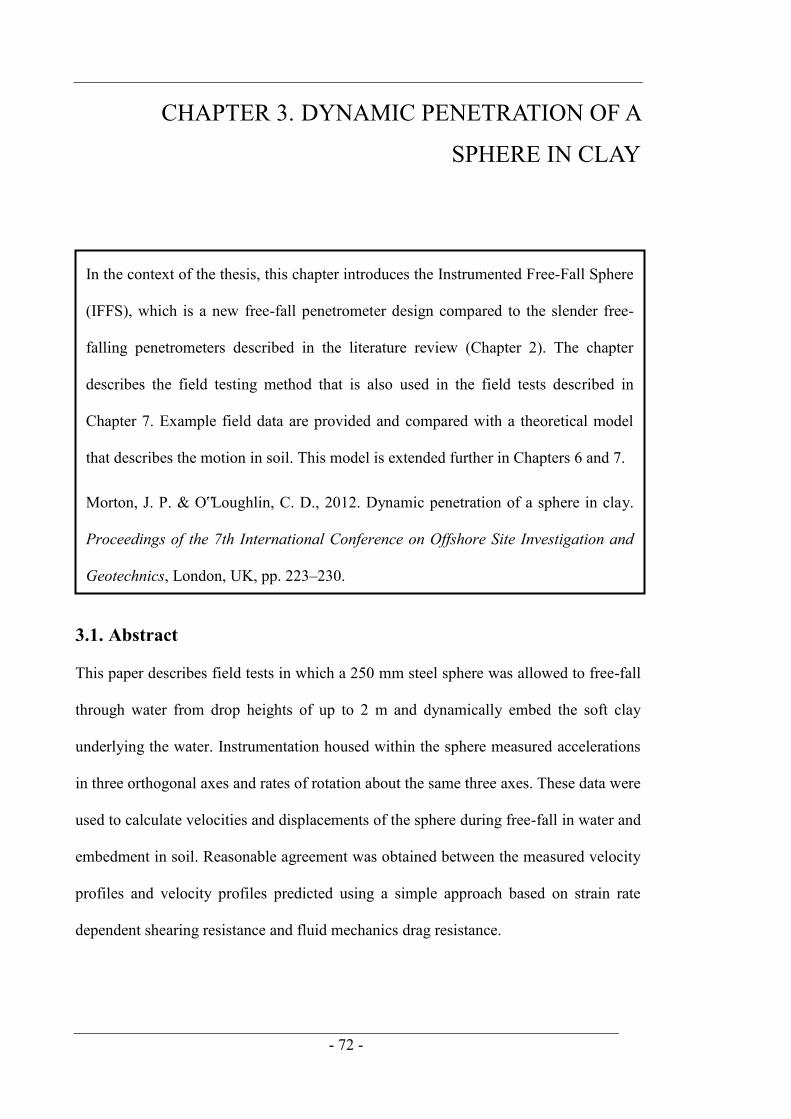
- 72 -
CHAPTER 3. DYNAMIC PENETRATION OF A
SPHERE IN CLAY
3.1. Abstract
This paper describes field tests in which a 250 mm steel sphere was allowed to free-fall
through water from drop heights of up to 2 m and dynamically embed the soft clay
underlying the water. Instrumentation housed within the sphere measured accelerations
in three orthogonal axes and rates of rotation about the same three axes. These data were
used to calculate velocities and displacements of the sphere during free-fall in water and
embedment in soil. Reasonable agreement was obtained between the measured velocity
profiles and velocity profiles predicted using a simple approach based on strain rate
dependent shearing resistance and fluid mechanics drag resistance.
In the context of the thesis, this chapter introduces the Instrumented Free-Fall Sphere
(IFFS), which is a new free-fall penetrometer design compared to the slender free-
falling penetrometers described in the literature review (Chapter 2). The chapter
describes the field testing method that is also used in the field tests described in
Chapter 7. Example field data are provided and compared with a theoretical model
that describes the motion in soil. This model is extended further in Chapters 6 and 7.
Morton, J. P. & O‟Loughlin, C. D., 2012. Dynamic penetration of a sphere in clay.
Proceedings of the 7th International Conference on Offshore Site Investigation and
Geotechnics, London, UK, pp. 223–230.
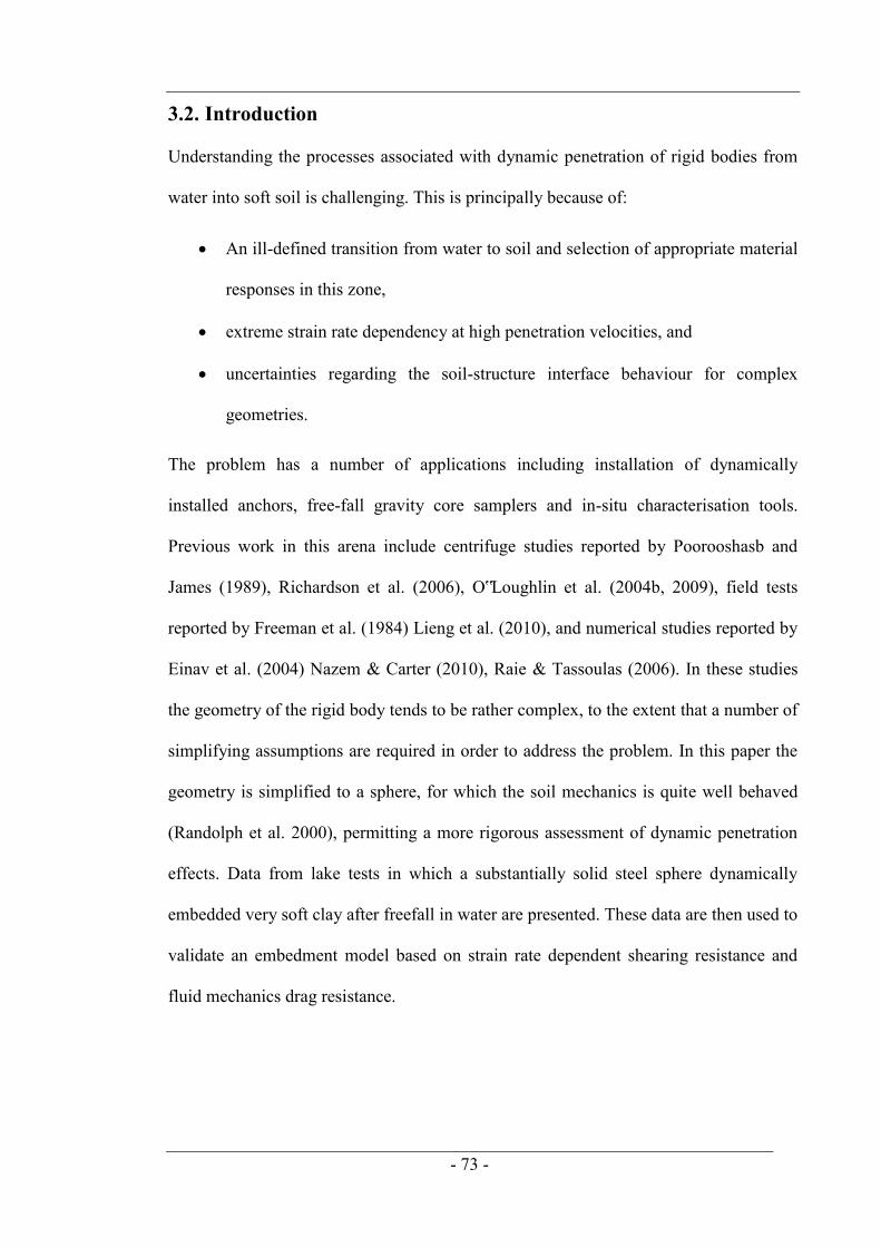
- 73 -
3.2. Introduction
Understanding the processes associated with dynamic penetration of rigid bodies from
water into soft soil is challenging. This is principally because of:
An ill-defined transition from water to soil and selection of appropriate material
responses in this zone,
extreme strain rate dependency at high penetration velocities, and
uncertainties regarding the soil-structure interface behaviour for complex
geometries.
The problem has a number of applications including installation of dynamically
installed anchors, free-fall gravity core samplers and in-situ characterisation tools.
Previous work in this arena include centrifuge studies reported by Poorooshasb and
James (1989), Richardson et al. (2006), O‟Loughlin et al. (2004b, 2009), field tests
reported by Freeman et al. (1984) Lieng et al. (2010), and numerical studies reported by
Einav et al. (2004) Nazem & Carter (2010), Raie & Tassoulas (2006). In these studies
the geometry of the rigid body tends to be rather complex, to the extent that a number of
simplifying assumptions are required in order to address the problem. In this paper the
geometry is simplified to a sphere, for which the soil mechanics is quite well behaved
(Randolph et al. 2000), permitting a more rigorous assessment of dynamic penetration
effects. Data from lake tests in which a substantially solid steel sphere dynamically
embedded very soft clay after freefall in water are presented. These data are then used to
validate an embedment model based on strain rate dependent shearing resistance and
fluid mechanics drag resistance.

- 74 -
3.3. Site description and soil properties
3.3.1. Site location and description
Tests were conducted in Lower Lough Erne, Northern Ireland (see Figure 3.1). The lake
is the third largest lake in Britain and Ireland with an area of 109 km2 and is part of the
complex Erne system, with a catchment of 4212 km2.
Figure 3.1. Site location and bathymetric map of Lower Lough Erne (after
Lafferty et al. 2006)
The lower lake, which is situated in County Fermanagh, is located in a deep glacial
trough. The lakebed is largely composed of fine-grained sediments and limestone debris
of boulder clay (Lafferty et al. 2006). At the test site the lakebed is extremely soft to
depths of at least 8 m (Colreavy et al. 2012) and the superficial deposits are principally
underlain by Carboniferous Limestone (Gibson, 1998).
3.3.2. Soil classification
A number of bulk excavated samples have been obtained from the test site from depths
up to 2.5 m and some preliminary classification tests have been carried out. Initial
results are outside the range normally expected for soft clays. Natural moisture contents
are high throughout with values in the range of 270–520%. The Atterberg limits are also

- 75 -
high with plastic limits of 130–180% and liquid limits of 250–315%. Plasticity index
values are in the range of 120–175%. In all cases, the moisture content was
approximately 1.5 times the liquid limit. Over the depth of interest, the unit weight is
constant with depth and only marginally higher than that of water at 10.5 kN/m3.
Scanning electron microscopy images of oven dried samples of the clay revealed
significant amounts of diatoms and other unidentified microfossils (Colreavy et al.
2012). The presence of these microfossils is known to influence soil behaviour, and
contributes to high liquid limits, high porosity, and unusual compressibility (Mitchell &
Soga, 2005). Similar unusual characteristics and index properties have also been
reported for Mexico City clay, which also contains significant amounts of microfossils
(Mesri et al. 1975, Diaz-Rodriguez et al. 1998).
3.3.3. Shear strength profiles
(Colreavy et al. 2012) present penetration data from T-bar and piezoball tests conducted
at the testing site to depths of up to 8m. The penetration tests were performed using a
light weight cone penetrometer testing rig mounted on a floating pontoon. All
penetration tests were conducted at the standard penetration rate of 20 mm/s in an
attempt to ensure undrained conditions. Typical undrained shear strength profiles are
provided on Figure 3.2 for the upper 2 m as this is the depth of interest for the dynamic
penetration tests. The data on Figure 3.2 have been interpreted from the net penetration
data reported by Colreavy et al. (2012) using the commonly adopted resistance factor N
= 10.5 (DeJong et al. 2004, Chung & Randolph, 2004). These strength profiles represent
an undrained shear strength gradient, k = 1.4 kPa/m which is in the range considered
typical for deep water sediments (Randolph, 2004).
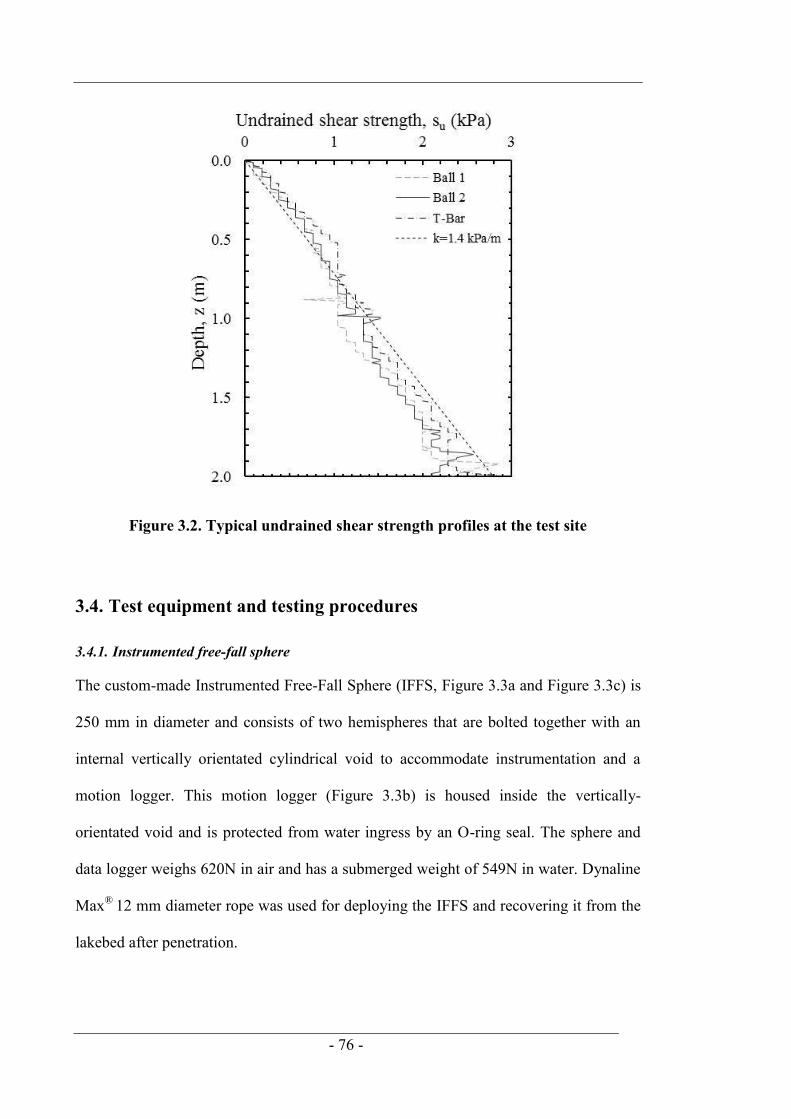
- 76 -
Figure 3.2. Typical undrained shear strength profiles at the test site
3.4. Test equipment and testing procedures
3.4.1. Instrumented free-fall sphere
The custom-made Instrumented Free-Fall Sphere (IFFS, Figure 3.3a and Figure 3.3c) is
250 mm in diameter and consists of two hemispheres that are bolted together with an
internal vertically orientated cylindrical void to accommodate instrumentation and a
motion logger. This motion logger (Figure 3.3b) is housed inside the vertically-
orientated void and is protected from water ingress by an O-ring seal. The sphere and
data logger weighs 620N in air and has a submerged weight of 549N in water. Dynaline
Max® 12 mm diameter rope was used for deploying the IFFS and recovering it from the
lakebed after penetration.
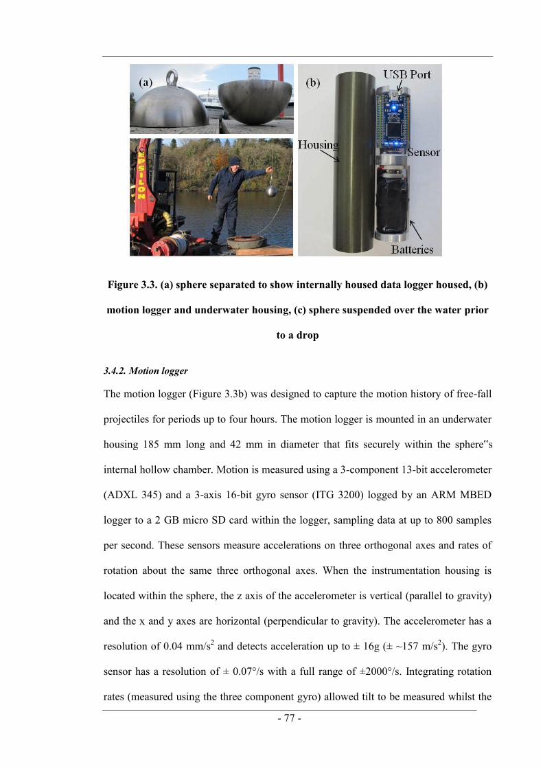
- 77 -
Figure 3.3. (a) sphere separated to show internally housed data logger housed, (b)
motion logger and underwater housing, (c) sphere suspended over the water prior
to a drop
3.4.2. Motion logger
The motion logger (Figure 3.3b) was designed to capture the motion history of free-fall
projectiles for periods up to four hours. The motion logger is mounted in an underwater
housing 185 mm long and 42 mm in diameter that fits securely within the sphere‟s
internal hollow chamber. Motion is measured using a 3-component 13-bit accelerometer
(ADXL 345) and a 3-axis 16-bit gyro sensor (ITG 3200) logged by an ARM MBED
logger to a 2 GB micro SD card within the logger, sampling data at up to 800 samples
per second. These sensors measure accelerations on three orthogonal axes and rates of
rotation about the same three orthogonal axes. When the instrumentation housing is
located within the sphere, the z axis of the accelerometer is vertical (parallel to gravity)
and the x and y axes are horizontal (perpendicular to gravity). The accelerometer has a
resolution of 0.04 mm/s2 and detects acceleration up to ± 16g (± ~157 m/s2). The gyro
sensor has a resolution of ± 0.07°/s with a full range of ±2000°/s. Integrating rotation
rates (measured using the three component gyro) allowed tilt to be measured whilst the

- 78 -
IFFS was accelerating in water or decelerating in soil. These measurements were used
to adjust the accelerations measured on the z axis of the accelerometer so that they
correspond to the accelerations in the vertical plane.
3.4.3. Field testing procedure
The sphere was deployed from various drop heights so as to examine the embedment
response of the sphere over a range of impact velocities. Depending on the required
release height above the lakebed, the experiments were conducted either from a jetty, a
floating pontoon or a self-propelled hopper barge. Care was taken to ensure that each
installation site was at least 2 m (8 sphere diameters) from existing test sites. In each
test a portable crane (for the jetty and pontoon tests) or a fixed crane (for the barge tests)
was used to suspend the IFFS at the pre-selected release height, and release was
achieved using a quick release shackle. The embedment depth of the IFFS was
measured by lowering a submersible camera positioned on a weighted platform so as to
focus on known markings on the retrieval rope.
3.5. Test results and analysis
3.5.1. Acceleration profile
A typical acceleration trace, calculated from the horizontally-orientated x and y axes
and the vertically-orientated z axis is shown in Figure 3.4. The z axis acceleration trace
changes abruptly at 0.3s, from 0 m/s2 when hanging vertically in water to ~10 m/s2 after
the quick release shackle was pulled and the IFFS started to free-fall. During free-fall,
the net acceleration decreases as drag on the sphere increases with increasing velocity.
Impact at the lakebed is apparent at ~0.6s, when the sphere decelerates rapidly and then
comes to rest at ~1.4s before rebounding slightly. This rebound is thought to be due to
the stored elastic energy in the clay. Similar results have been reported in free-fall
experiments (e.g. Dayal & Allen, 1973, Chow & Airey, 2010).

- 79 -
The horizontally-orientated y axis accelerometer trace indicates that the sphere rotated
during penetration in soil as the y axis trace does not return to the same position as
before the test (when hanging vertically in water, ~0 m/s2). Rotation derived from the
horizontally-orientated x and y axes of the tri-axis accelerometer is compared with the
rotation derived from the x and y axes of the gyro sensor in Figure 3.4. During the test
the angle of rotation was less than 3° in the x axis, whereas the sphere rotated steadily to
15° in the y axis. This rotation highlights the need to adjust the accelerations measured
on the z axis of the accelerometer during free-fall in water and penetration of the
lakebed.

- 80 -
Figure 3.4. (a) x, y and z axis acceleration traces from a typical test, (b) x and y
axis rotation traces from the same test
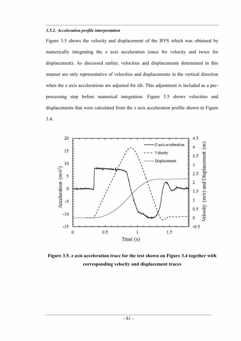
- 81 -
3.5.2. Acceleration profile interpretation
Figure 3.5 shows the velocity and displacement of the IFFS which was obtained by
numerically integrating the z axis acceleration (once for velocity and twice for
displacement). As discussed earlier, velocities and displacements determined in this
manner are only representative of velocities and displacements in the vertical direction
when the z axis accelerations are adjusted for tilt. This adjustment is included as a pre-
processing step before numerical integration. Figure 3.5 shows velocities and
displacements that were calculated from the z axis acceleration profile shown in Figure
3.4.
Figure 3.5. z axis acceleration trace for the test shown on Figure 3.4 together with
corresponding velocity and displacement traces

- 82 -
3.5.3. Velocity and embedment depth profile
Figure 3.6 shows the velocity–embedment depth profiles for a 0.5 m and a 1 m release
height above the lakebed. The profiles show the velocity increasing from 0 m/s at the
release height to ~3 m/s and ~4 m/s for the 0.5 m and 1 m drop heights respectively. As
is to be expected for low drop heights (≤ 4 sphere diameters), the velocity does not
reach terminal velocity in water and actually continues to increase during initial
penetration of the soil. This is due to the very low resistance afforded by the very soft
sediments near the lakebed surface. At some depth the resistance available from the soil
exceeds the submerged weight of the sphere and the sphere begins to decelerate. Similar
profiles have been reported by O‟Loughlin et al. (2009) from centrifuge tests on
dynamically installed anchors. Ultimately the sphere comes to rest in the soil as
indicated by zero velocity (in the lakebed) on. This eventual embedment depth is 1.15 m
and 1.35 m for the 0.5 m and 1.0 m drop heights and is in agreement with independent
direct sight measurements using the underwater camera (see Figure 3.7). The
availability of continuous velocity profiles such as that on Figure 3.6 allows embedment
prediction models to be verified and calibrated. The second half of this paper describes
such an embedment model and uses the data reported here to assess its performance.
3.6. Embedment depth prediction
The embedment of bodies penetrating soil after free-fall in water may be quantified by
considering Newton‟s second law of motion and the forces acting on the body during
penetration. Several studies (e.g. True, 1976, Aubeny & Shi, 2006, Audibert et al. 2006,
O‟Loughlin et al. 2004a) have adopted such an approach, with variations on the
inclusion and formulation of the various forces acting on the body during penetration. A
similar approach is adopted here with the forces acting on the body during penetration
shown by Figure 3.8, leading to a governing equation of:

- 83 -
dbfs FFRWdt
zdm 2
2
3.1
where m is the sphere mass, z is the penetration depth below the lakebed, t is the time
after impact with the soil, Ws is the submerged weight of the sphere in clay, Rf is a
strain rate function, Fb is the bearing resistance and Fd is the drag resistance. The
inclusion of the strain rate function, Rf, is justified as the shear strength of clays is well
known to be a function of strain rate (Casagrande & Wilson, 1951, Graham et al. 1983).
Figure 3.6. Velocity profiles in water and soil for release heights of 0.5 m and 1 m
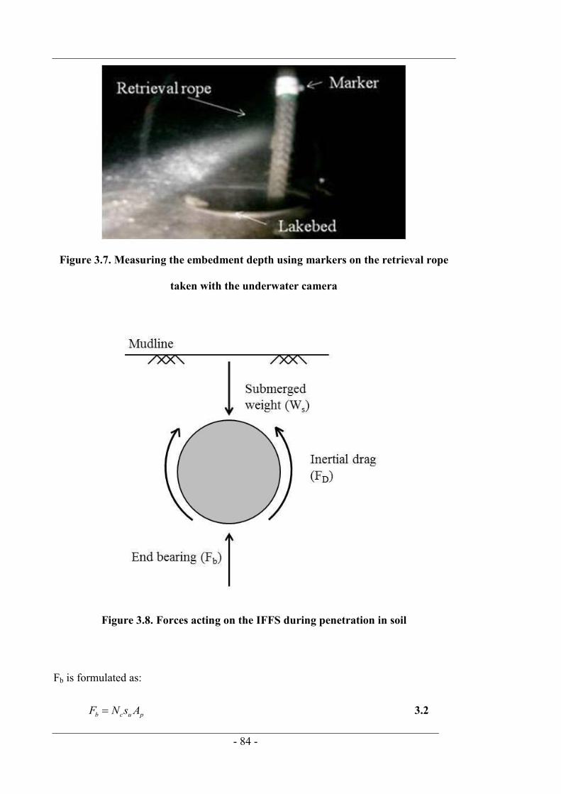
- 84 -
Figure 3.7. Measuring the embedment depth using markers on the retrieval rope
taken with the underwater camera
Figure 3.8. Forces acting on the IFFS during penetration in soil
Fb is formulated as:
pucb AsNF 3.2
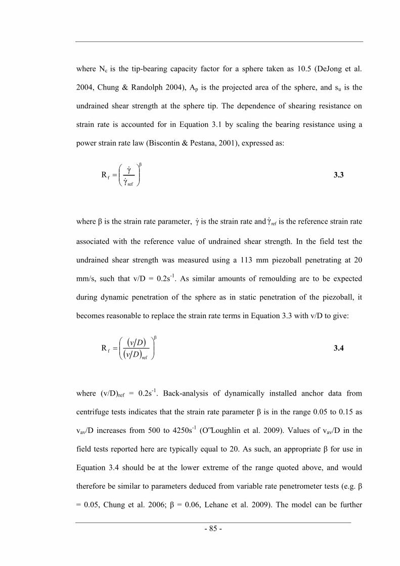
- 85 -
where Nc is the tip-bearing capacity factor for a sphere taken as 10.5 (DeJong et al.
2004, Chung & Randolph 2004), Ap is the projected area of the sphere, and su is the
undrained shear strength at the sphere tip. The dependence of shearing resistance on
strain rate is accounted for in Equation 3.1 by scaling the bearing resistance using a
power strain rate law (Biscontin & Pestana, 2001), expressed as:
β
reff γ
γR
3.3
where β is the strain rate parameter, γ is the strain rate and refγ is the reference strain rate
associated with the reference value of undrained shear strength. In the field test the
undrained shear strength was measured using a 113 mm piezoball penetrating at 20
mm/s, such that v/D = 0.2s-1. As similar amounts of remoulding are to be expected
during dynamic penetration of the sphere as in static penetration of the piezoball, it
becomes reasonable to replace the strain rate terms in Equation 3.3 with v/D to give:
β
reffR
DvDv
3.4
where (v/D)ref = 0.2s-1. Back-analysis of dynamically installed anchor data from
centrifuge tests indicates that the strain rate parameter β is in the range 0.05 to 0.15 as
vav/D increases from 500 to 4250s-1 (O‟Loughlin et al. 2009). Values of vav/D in the
field tests reported here are typically equal to 20. As such, an appropriate β for use in
Equation 3.4 should be at the lower extreme of the range quoted above, and would
therefore be similar to parameters deduced from variable rate penetrometer tests (e.g. β
= 0.05, Chung et al. 2006; β = 0.06, Lehane et al. 2009). The model can be further
- 86 -
refined by accounting for the transition from a shallow to a deep failure mechanism
during shallow penetration and also for the buoyancy effects as the ball transitions from
water into soil (White et al. 2010). However these refinements are not warranted here as
the unit weight of the soil is close to that of water and the ball typically embeds by
several diameters.
The inclusion of the fluid mechanics drag term, Fd, in Equation 3.1 is warranted in view
of the very soft viscous clay that is often encountered at the clay surface (O‟Loughlin et
al. 2009). The fluid drag is formulated as:
2
21 vACF pDd 3.5
where CD is the drag coefficient, dictated largely by object geometry (blunt objects
exhibit a large CD and streamlined bodies exhibit smaller CD), ρ is the density of the
soil, Ap is the projected area and v is the velocity.
An appropriate CD for the sphere can be determined by considering Equation 3.1 during
freefall in water rather than embedment in soil. As such the bearing resistance term in
Equation 3.1 becomes zero, the submerged weight, Ws, (in Equation 3.1) and the
density, ρ, relate to water rather than soil. The governing equation in water then
becomes:
2
22
21
dtzdmvACW pds 3.6
The theoretical velocity profile for the sphere free falling in water can then be
constructed from a finite difference approximation of Equation 3.6. These theoretical
profiles are shown on Figure 3.9 together with experimental velocity profiles for drop
heights of 0.5m, 1 m and 2 m. Lower and upper bounds to the experimental data are
obtained using CD = 0.3 and CD = 0.4, with an average CD = 0.35 providing the best
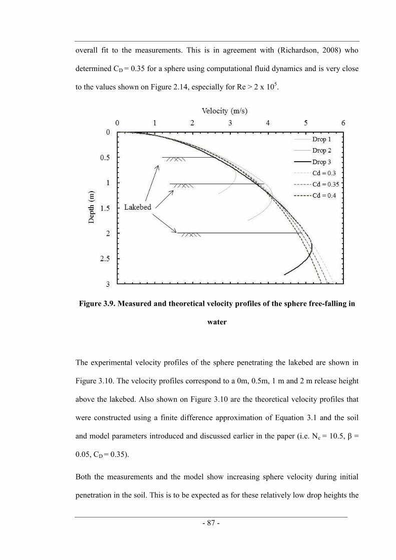
- 87 -
overall fit to the measurements. This is in agreement with (Richardson, 2008) who
determined CD = 0.35 for a sphere using computational fluid dynamics and is very close
to the values shown on Figure 2.14, especially for Re > 2 x 10⁵.
Figure 3.9. Measured and theoretical velocity profiles of the sphere free-falling in
water
The experimental velocity profiles of the sphere penetrating the lakebed are shown in
Figure 3.10. The velocity profiles correspond to a 0m, 0.5m, 1 m and 2 m release height
above the lakebed. Also shown on Figure 3.10 are the theoretical velocity profiles that
were constructed using a finite difference approximation of Equation 3.1 and the soil
and model parameters introduced and discussed earlier in the paper (i.e. Nc = 10.5, β =
0.05, CD = 0.35).
Both the measurements and the model show increasing sphere velocity during initial
penetration in the soil. This is to be expected as for these relatively low drop heights the
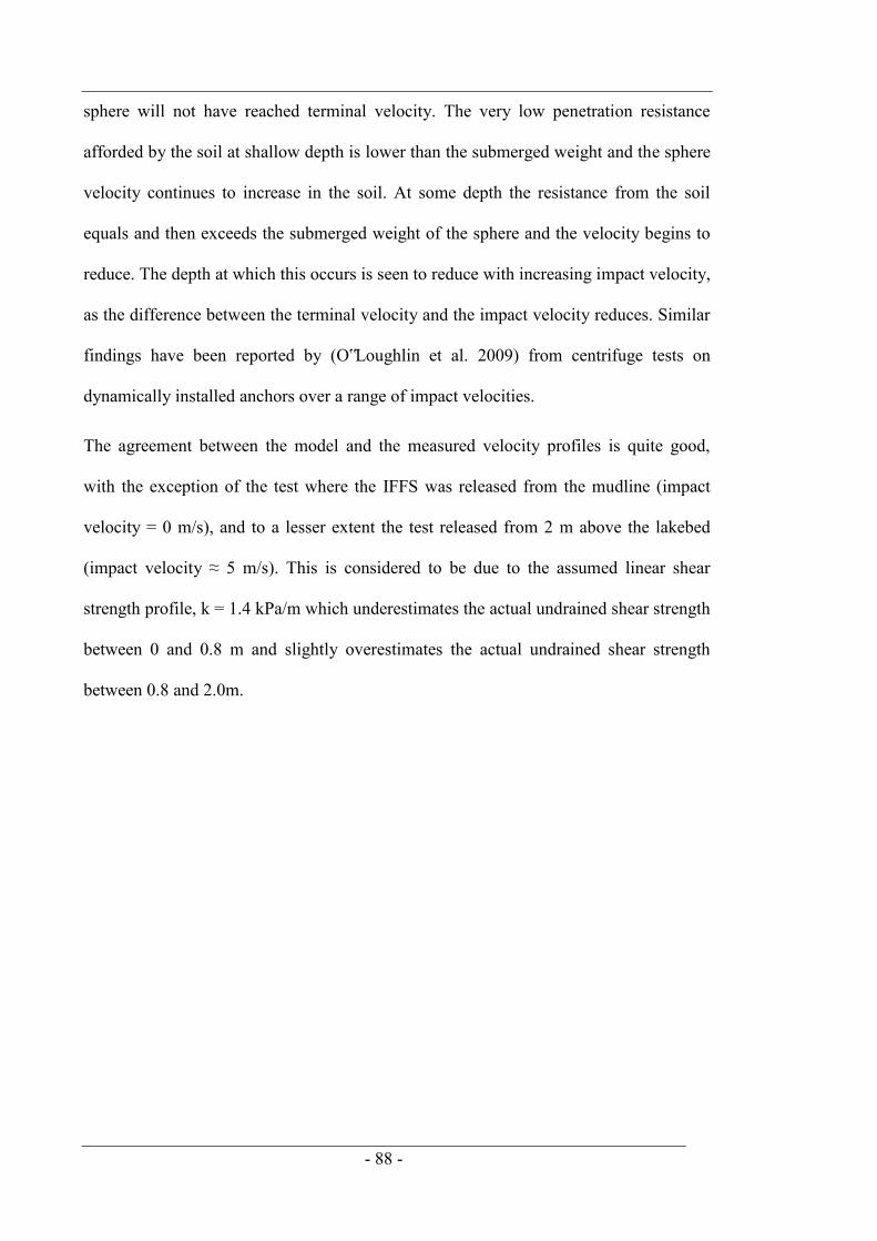
- 88 -
sphere will not have reached terminal velocity. The very low penetration resistance
afforded by the soil at shallow depth is lower than the submerged weight and the sphere
velocity continues to increase in the soil. At some depth the resistance from the soil
equals and then exceeds the submerged weight of the sphere and the velocity begins to
reduce. The depth at which this occurs is seen to reduce with increasing impact velocity,
as the difference between the terminal velocity and the impact velocity reduces. Similar
findings have been reported by (O‟Loughlin et al. 2009) from centrifuge tests on
dynamically installed anchors over a range of impact velocities.
The agreement between the model and the measured velocity profiles is quite good,
with the exception of the test where the IFFS was released from the mudline (impact
velocity = 0 m/s), and to a lesser extent the test released from 2 m above the lakebed
(impact velocity ≈ 5 m/s). This is considered to be due to the assumed linear shear
strength profile, k = 1.4 kPa/m which underestimates the actual undrained shear strength
between 0 and 0.8 m and slightly overestimates the actual undrained shear strength
between 0.8 and 2.0m.
- 89 -
Figure 3.10. Predicted and measured velocity profiles of the sphere penetrating the
lakebed
3.7. Conclusions
This paper has presented field tests undertaken to evaluate the behaviour of a simple
geometry dynamically penetrating soft clay. The tests, which were undertaken in a lake
in water depths up to 5m, involved the release of a substantially solid steel sphere, 250
mm in diameter, through drop heights of up to 2m. Impact velocities (at the mudline) of
up to 5.1 m/s were obtained in the field tests, resulting in embedment (to the base of the
sphere) of 1.52 m, equivalent to over 6 sphere diameters. Reasonable agreement was
obtained between the measured velocity profiles and velocity profiles predicted using a
simple approach based on strain rate dependent shearing resistance (β = 0.05) and fluid
mechanics drag resistance (CD = 0.35).
- 90 -
CHAPTER 4. STRENGTH ASSESSMENT DURING
SHALLOW PENETRATION OF A SPHERE IN CLAY
4.1. Abstract
Strength interpretation from the measured penetration resistance of full-flow
penetrometers, such as the T-bar and ball, is generally based on a constant bearing
capacity factor associated with a deep flow-round mechanism. This approach may
underestimate the strength of near-surface sediments, which is becoming increasingly
important for the design of offshore infrastructure such as pipelines, steel catenary risers
The theoretical model considered in Chapter 3 makes the limiting assumption that
shallow penetration effects may be ignored. This chapter avoids this limitation by
proposing a shallow penetration framework that more accurately determines the
penetration resistance acting on a ball penetrometer whether pushed in or free-falling
during shallow embedment. The framework is used in Chapters 7 and 8 where it is
applied to field and centrifuge experiments for the analysis of push-in and free-falling
ball penetrometer tests.
Morton, J. P., O‟Loughlin, C. D. & White. D. J., 2014. Strength assessment during
shallow penetration of a sphere in clay. Géotechnique Letters 4 (October-December),
pp. 262–266.
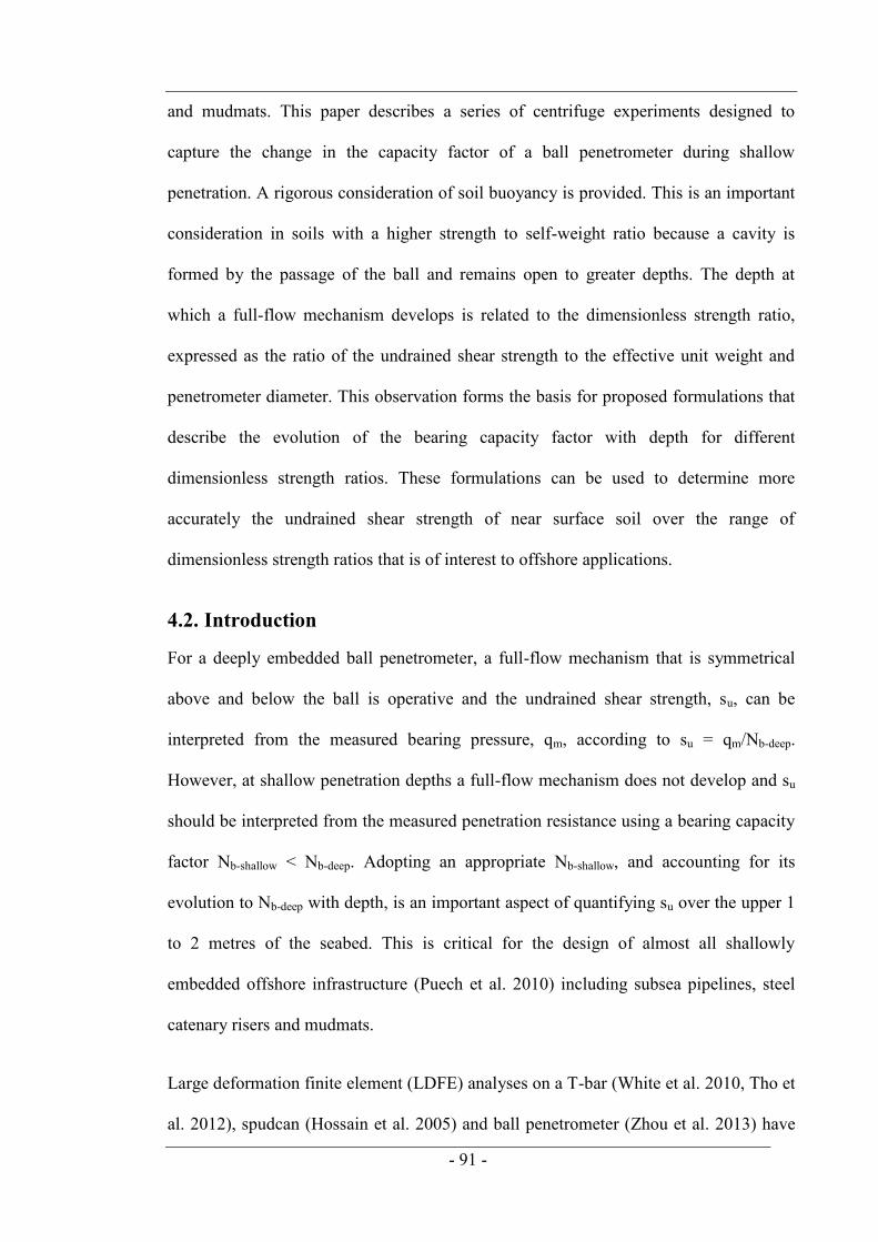
- 91 -
and mudmats. This paper describes a series of centrifuge experiments designed to
capture the change in the capacity factor of a ball penetrometer during shallow
penetration. A rigorous consideration of soil buoyancy is provided. This is an important
consideration in soils with a higher strength to self-weight ratio because a cavity is
formed by the passage of the ball and remains open to greater depths. The depth at
which a full-flow mechanism develops is related to the dimensionless strength ratio,
expressed as the ratio of the undrained shear strength to the effective unit weight and
penetrometer diameter. This observation forms the basis for proposed formulations that
describe the evolution of the bearing capacity factor with depth for different
dimensionless strength ratios. These formulations can be used to determine more
accurately the undrained shear strength of near surface soil over the range of
dimensionless strength ratios that is of interest to offshore applications.
4.2. Introduction
For a deeply embedded ball penetrometer, a full-flow mechanism that is symmetrical
above and below the ball is operative and the undrained shear strength, su, can be
interpreted from the measured bearing pressure, qm, according to su = qm/Nb-deep.
However, at shallow penetration depths a full-flow mechanism does not develop and su
should be interpreted from the measured penetration resistance using a bearing capacity
factor Nb-shallow < Nb-deep. Adopting an appropriate Nb-shallow, and accounting for its
evolution to Nb-deep with depth, is an important aspect of quantifying su over the upper 1
to 2 metres of the seabed. This is critical for the design of almost all shallowly
embedded offshore infrastructure (Puech et al. 2010) including subsea pipelines, steel
catenary risers and mudmats.
Large deformation finite element (LDFE) analyses on a T-bar (White et al. 2010, Tho et
al. 2012), spudcan (Hossain et al. 2005) and ball penetrometer (Zhou et al. 2013) have

- 92 -
shown that the transition depth from Nb-shallow to Nb-deep is dependent on the
dimensionless strength ratio, su/γ'D, where γ' is the effective unit weight of the soil and
D is the diameter of the penetrometer. Higher strength ratios are associated with a delay
in the transition to a steady Nb-deep. Correlations for the transition depth and Nb-shallow
have been derived and, in the case of the T-bar and ball, a basis for correcting
penetration data within the shallow zone has been proposed (White et al. 2010, Zhou et
al. 2013). However from the perspective of a spherical penetrometer, which is the focus
of this paper, the range of strength ratios previously examined (su/γ'D = 2.95 to 44.25,
Zhou et al. 2013) is narrower than the range that is of practical interest for offshore
problems. For example, a 250 mm diameter freefall spherical penetrometer (for
measuring the strength of the seabed, Morton & O‟Loughlin, 2012) penetrating very
soft soil is associated with low values of su/γ'D approaching 0.1 at one diameter
embedment, whereas an 80 mm piezoball penetrating the seabed with a crust strength of
~20 kPa is associated with high values of su/γ'D, approaching 40.
The motivation for this study was to experimentally capture the variation in Nb-shallow
with depth for a ball penetrometer embedding into clay over a wide range of su/γ'D. The
experimental data are combined with reinterpreted LDFE results (Zhou et al. 2013), and
form the basis of a new correlation which describes the evolution of Nb with depth.
4.3. Experimental details
The problem is addressed through centrifuge tests carried out at 100 g in the University
of Western Australia (UWA) beam centrifuge. The penetration resistance response and
the degree of hole-closure were analysed for nine penetrometer tests using a 11.3 mm
diameter ball with a 4.8 mm diameter shaft, penetrating a kaolin clay sample with a
progressively higher overconsolidation ratio. A constant penetration rate of 1 mm/s was
adopted such that the non-dimensional velocity, vD/cv ~ 130 (where v is the penetration

- 93 -
rate, D is the sphere diameter, and cv is the coefficient of vertical consolidation ~ 2.8
m2/yr (Cocjin et al. 2014) and the response is primarily undrained (House et al. 2001).
A video observed the progressive hole-closure during each test, and provided a means
of determining the depth at which the cavity, formed by the passage of the ball, closed
over. The experimental arrangement is shown in Figure 4.1.
4.4. Experimental procedure
4.4.1. Preparation of clay specimen
The sample was prepared by mixing kaolin powder with water in a vacuum mixer at a
moisture content equal to twice the liquid limit (120%). A drainage sand layer at the
base of the sample allowed two-way drainage during self-weight consolidation in the
centrifuge at 100 g, and vertical drains in the corners of the sample ensured there was no
hydraulic gradient over the height of the sample. A nominal 10 mm layer of free water
was maintained throughout testing.
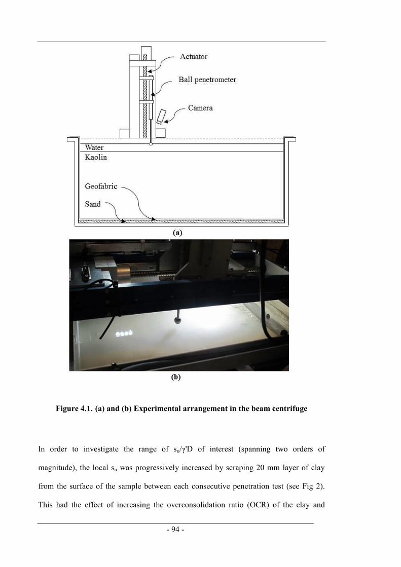
- 94 -
Figure 4.1. (a) and (b) Experimental arrangement in the beam centrifuge
In order to investigate the range of su/γ'D of interest (spanning two orders of
magnitude), the local su was progressively increased by scraping 20 mm layer of clay
from the surface of the sample between each consecutive penetration test (see Fig 2).
This had the effect of increasing the overconsolidation ratio (OCR) of the clay and

- 95 -
increasing su relative to the (new) sample surface. In order to minimise potential
boundary effects, a minimum of 3 sphere diameters was allowed between each test site
and sample walls.
Figure 4.2. A scraped soil sample before a test
Figure 4.3. Ball penetrometer and cavity after a penetration test
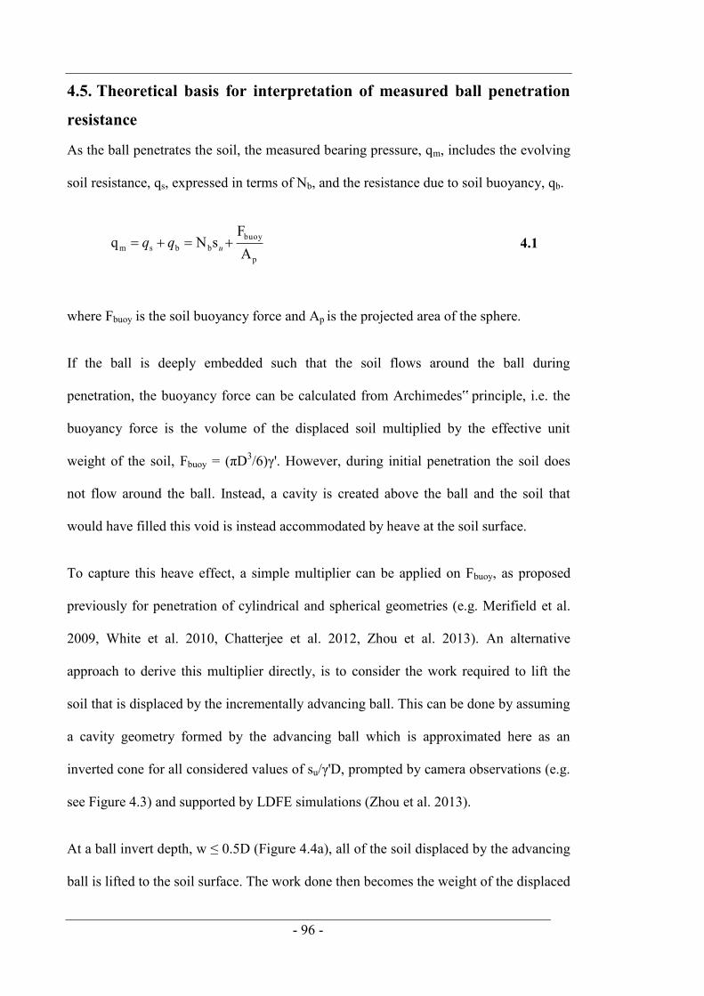
- 96 -
4.5. Theoretical basis for interpretation of measured ball penetration
resistance
As the ball penetrates the soil, the measured bearing pressure, qm, includes the evolving
soil resistance, qs, expressed in terms of Nb, and the resistance due to soil buoyancy, qb.
p
buoybbsm A
FsNq uqq 4.1
where Fbuoy is the soil buoyancy force and Ap is the projected area of the sphere.
If the ball is deeply embedded such that the soil flows around the ball during
penetration, the buoyancy force can be calculated from Archimedes‟ principle, i.e. the
buoyancy force is the volume of the displaced soil multiplied by the effective unit
weight of the soil, Fbuoy = (πD3/6)γ'. However, during initial penetration the soil does
not flow around the ball. Instead, a cavity is created above the ball and the soil that
would have filled this void is instead accommodated by heave at the soil surface.
To capture this heave effect, a simple multiplier can be applied on Fbuoy, as proposed
previously for penetration of cylindrical and spherical geometries (e.g. Merifield et al.
2009, White et al. 2010, Chatterjee et al. 2012, Zhou et al. 2013). An alternative
approach to derive this multiplier directly, is to consider the work required to lift the
soil that is displaced by the incrementally advancing ball. This can be done by assuming
a cavity geometry formed by the advancing ball which is approximated here as an
inverted cone for all considered values of su/γ'D, prompted by camera observations (e.g.
see Figure 4.3) and supported by LDFE simulations (Zhou et al. 2013).
At a ball invert depth, w ≤ 0.5D (Figure 4.4a), all of the soil displaced by the advancing
ball is lifted to the soil surface. The work done then becomes the weight of the displaced
- 97 -
soil multiplied by the distance between the centroidal height of the embedded ball (a
spherical cap) and the soil surface. For 0.5D > w ≤ Hc + D, where Hc is the cavity depth,
only some of the soil displaced by the advancing ball is lifted to the surface. The
remainder fills part of the cavity created by the increment of ball penetration as shown
in Figure 4.4b. In this case, the work done is calculated by adding the gain in potential
energy by these two separate elements of soil, resulting in the profile of soil buoyancy
with embedment given in Figure 4.4c. The analytical closed-form solution to calculate
the soil buoyancy is shown in Appendix 1.

- 98 -
Figure 4.4. Schematic illustration of soil buoyancy due to (a) the sphere and (b) the
sphere and conical cavity (c) buoyancy function for a typical cavity depth
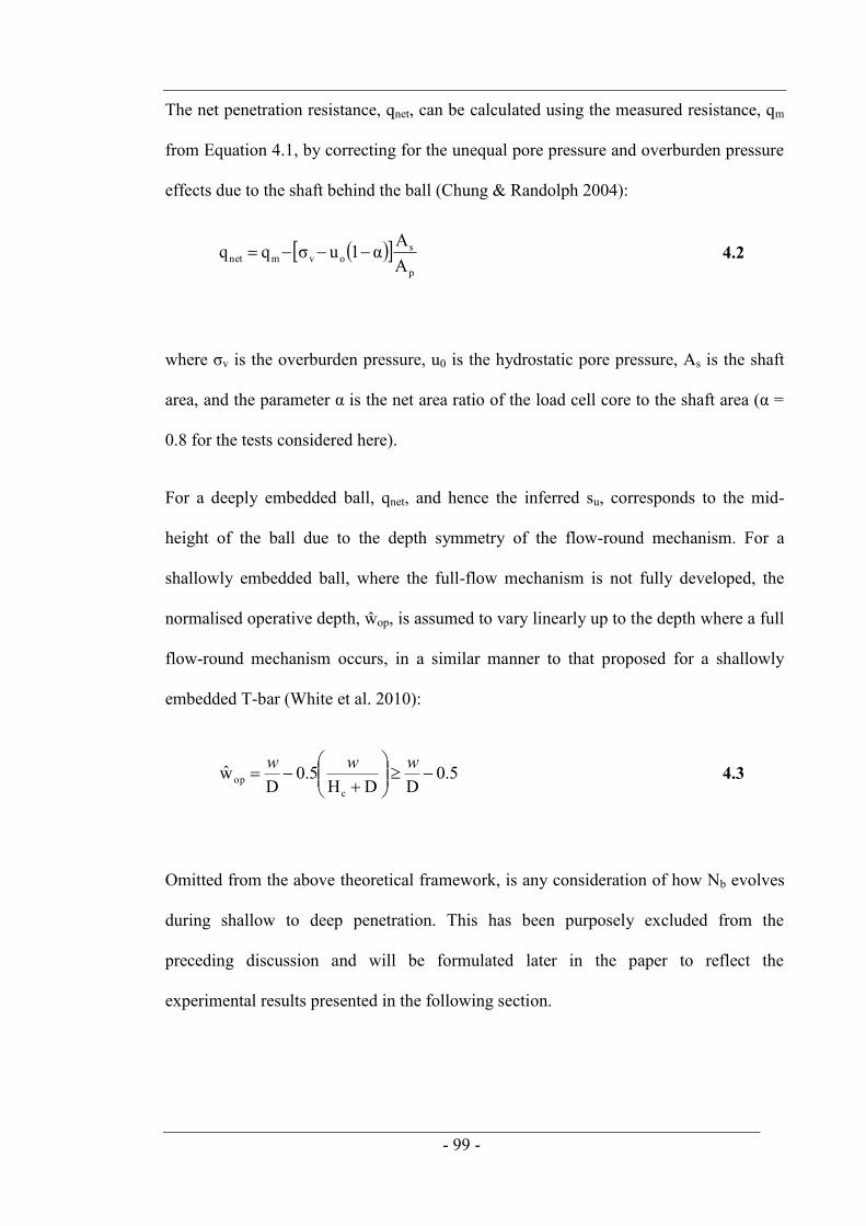
- 99 -
The net penetration resistance, qnet, can be calculated using the measured resistance, qm
from Equation 4.1, by correcting for the unequal pore pressure and overburden pressure
effects due to the shaft behind the ball (Chung & Randolph 2004):
p
sovmnet A
Aα1uσqq 4.2
where σv is the overburden pressure, u0 is the hydrostatic pore pressure, As is the shaft
area, and the parameter α is the net area ratio of the load cell core to the shaft area (α =
0.8 for the tests considered here).
For a deeply embedded ball, qnet, and hence the inferred su, corresponds to the mid-
height of the ball due to the depth symmetry of the flow-round mechanism. For a
shallowly embedded ball, where the full-flow mechanism is not fully developed, the
normalised operative depth, ŵop, is assumed to vary linearly up to the depth where a full
flow-round mechanism occurs, in a similar manner to that proposed for a shallowly
embedded T-bar (White et al. 2010):
0.5DDH
0.5D
wc
op
www 4.3
Omitted from the above theoretical framework, is any consideration of how Nb evolves
during shallow to deep penetration. This has been purposely excluded from the
preceding discussion and will be formulated later in the paper to reflect the
experimental results presented in the following section.
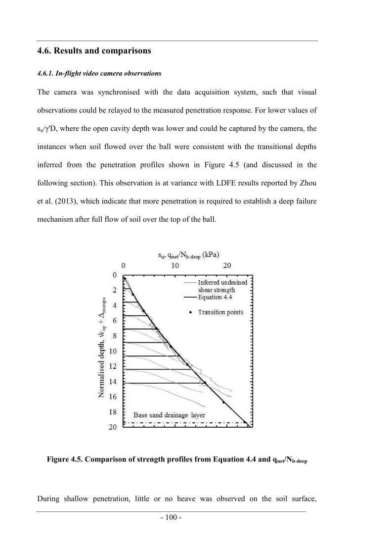
- 100 -
4.6. Results and comparisons
4.6.1. In-flight video camera observations
The camera was synchronised with the data acquisition system, such that visual
observations could be relayed to the measured penetration response. For lower values of
su/γ'D, where the open cavity depth was lower and could be captured by the camera, the
instances when soil flowed over the ball were consistent with the transitional depths
inferred from the penetration profiles shown in Figure 4.5 (and discussed in the
following section). This observation is at variance with LDFE results reported by Zhou
et al. (2013), which indicate that more penetration is required to establish a deep failure
mechanism after full flow of soil over the top of the ball.
Figure 4.5. Comparison of strength profiles from Equation 4.4 and qnet/Nb-deep
During shallow penetration, little or no heave was observed on the soil surface,
- 101 -
particularly for tests with higher values of su/γ'D. This is considered to be due to the
axisymmetric flow mechanism of the ball, which reduces the heave compared with
plane strain flow for a cylindrical T-bar or pipeline (Stanier & White, 2014). In light of
this observation, enhancement of Fbuoy in Equation 4.1 to account for heave of the soil
surface was included using the approach outlined in Section 4.5, and the approach
considered by Merifield et al. (2009), Randolph & White (2008) and Stanier & White
(2014) was not included.
4.6.2. Undrained shear strength profiles
As discussed earlier, the OCR of the sample was incrementally increased by scraping an
additional 20 mm from the sample surface between penetration tests. The strength of the
sample can then be assumed to vary with depth according to the following relationship
proposed by Ladd et al. (1977).
mOCRσsσs
ncv
uvu
4.4
where σ'v is the current vertical effective stress, determined from the γ' profile with
depth and the varying acceleration level within the centrifuge (93 to 105 g over the
depth of penetration) and m is the plastic volumetric strain ratio (Schofield and Wroth,
1968). The normally consolidated undrained strength ratio (su/σ'v)nc = 0.13, as
determined from ball penetrometer tests before scraping the soil surface (i.e. OCR = 1)
using the commonly adopted Nb-deep = 10.5 (Chung & Randolph 2004). The ratio
increases to (su/σ'v)nc = 0.15 if the measured resistance (which ignores shaft effects) is
considered, similar to (su/σ'v)nc = 0.16 reported by Richardson et al. (2009) and Hu et al.
(2014), and equivalent to an undrained strength gradient with prototype depth, k = 1
- 102 -
kPa/m, which is typical for UWA kaolin. The best agreement between Equation 4.4 and
the experimental qnet/Nb-deep profiles in the overconsolidated samples was obtained using
m = 1 (rather than the commonly reported m = 0.8), which reflects the minimal swelling
time permitted between each soil scrape and the subsequent penetration test.
4.6.3. Deep mechanism transition depth
The normalised transition depths, ŵdeep-op, are also shown on Figure 4.5, and were
selected as the depths where the qnet/Nb-deep experimental data were judged to have
reached su predicted using Equation 4.4. The final two profiles do not reach the
predicted su profile due to the proximity of the base drainage sand layer and ŵdeep-op are
approximated in these instances on the basis of the Nb variation with depth, discussed
below. Values of ŵdeep-op are also shown in Figure 4.6 alongside previously reported T-
bar, spudcan and ball data (White et al. 2010, Hossain et al. 2005 and Zhou et al. 2013
respectively), but re-interpreted to account for the definition of operative depth adopted
here. Further reinterpretation of the Zhou et al. (2013) ball data was made to ascertain
ŵdeep-op, assessed as when Nb became effectively constant (to within < 5% of the final
value), rather than reaching the limit, which is difficult to judge and is approached
asymptotically. The experimental ball data reported here, together with the reinterpreted
Zhou et al. (2013) ball data now form a unique relationship between ŵdeep-op and su/γ'D
for a ball penetrometer (where su is the undrained strength at ŵdeep-op), which can be
described using:
fu
cu
opdeep
eDγ's1
adDγ'
sbaw
4.5
where the fitting constants a = 16.3, b = 0.12, c = 1.3, d = 0.52, e = 4.9 and f = 1.5.
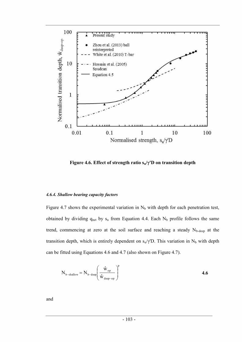
- 103 -
Figure 4.6. Effect of strength ratio su/γ'D on transition depth
4.6.4. Shallow bearing capacity factors
Figure 4.7 shows the experimental variation in Nb with depth for each penetration test,
obtained by dividing qnet by su from Equation 4.4. Each Nb profile follows the same
trend, commencing at zero at the soil surface and reaching a steady Nb-deep at the
transition depth, which is entirely dependent on su/γ'D. This variation in Nb with depth
can be fitted using Equations 4.6 and 4.7 (also shown on Figure 4.7).
p
opdeep
opdeepbshallowb w
wNN
4.6
and
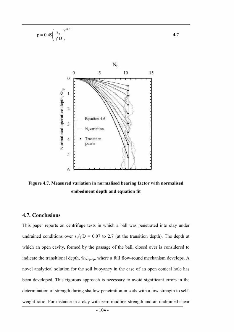
- 104 -
0.01u
Dγ's0.49p
4.7
Figure 4.7. Measured variation in normalised bearing factor with normalised
embedment depth and equation fit
4.7. Conclusions
This paper reports on centrifuge tests in which a ball was penetrated into clay under
undrained conditions over su/γ'D = 0.07 to 2.7 (at the transition depth). The depth at
which an open cavity, formed by the passage of the ball, closed over is considered to
indicate the transitional depth, ŵdeep-op, where a full flow-round mechanism develops. A
novel analytical solution for the soil buoyancy in the case of an open conical hole has
been developed. This rigorous approach is necessary to avoid significant errors in the
determination of strength during shallow penetration in soils with a low strength to self-
weight ratio. For instance in a clay with zero mudline strength and an undrained shear
- 105 -
strength ratio, su/σ'v = 0.25, the buoyancy resistance increases to almost 70% of the
geotechnical resistance during shallow penetration, and is independent of the
penetrometer diameter at all penetration depths. Data from the centrifuge experiments,
combined with reinterpreted data from LDFE analyses, show a unique relationship
between ŵdeep-op and su/γ'D examined over the range su/γ'D ≈ 0.1 to 40. Equations that
describe the change in ŵdeep-op and the capacity factor, Nb, with su/γ'D are proposed.
These equations offer a more rigorous and reliable means of assessing soil strength in
the upper few metres of the seabed.
- 106 -
CHAPTER 5. MEMS ACCELEROMETERS FOR
MEASURING DYNAMIC PENETRATION EVENTS IN
GEOTECHNICAL CENTRIFUGE TESTS
5.1. Abstract
Micro-electro mechanical system (MEMS) accelerometers are small, inexpensive
sensors that have only recently been used in geotechnical centrifuge tests. This is unlike
piezoelectric accelerometers, which are by comparison large and expensive but have
been used extensively in geotechnical centrifuge tests over the past couple of decades.
This paper examines the response of a single-axis ±500 g MEMS accelerometer under
both static and dynamic conditions in a centrifuge environment. The potential for
MEMS accelerometers to be used to measure the depth of objects buried in soil is
This chapter describes novel FFP experiments that use accelerometers embedded in a
reduced scale centrifuge model anchor to measure the motion response during free-
fall and embedment in soil. The chapter is a precursor for Chapters 6 and 8 where
further experiments with MEMS accelerometers are undertaken in the field and the
centrifuge. The chapter highlights the potential error associated with FFP tilt which is
investigated in more detail in Chapter 6.
O‟Loughlin, C. D., Gaudin, C., Morton. J. P. & White, D. J., 2014. MEMS
accelerometers for measuring dynamic penetration events in geotechnical centrifuge
tests International Journal of Physical Modelling in Geotechnics, 14(2), pp. 31–39.
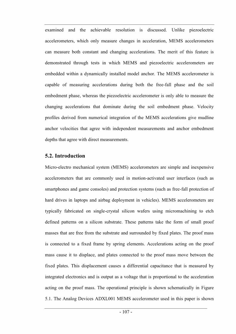
- 107 -
examined and the achievable resolution is discussed. Unlike piezoelectric
accelerometers, which only measure changes in acceleration, MEMS accelerometers
can measure both constant and changing accelerations. The merit of this feature is
demonstrated through tests in which MEMS and piezoelectric accelerometers are
embedded within a dynamically installed model anchor. The MEMS accelerometer is
capable of measuring accelerations during both the free-fall phase and the soil
embedment phase, whereas the piezoelectric accelerometer is only able to measure the
changing accelerations that dominate during the soil embedment phase. Velocity
profiles derived from numerical integration of the MEMS accelerations give mudline
anchor velocities that agree with independent measurements and anchor embedment
depths that agree with direct measurements.
5.2. Introduction
Micro-electro mechanical system (MEMS) accelerometers are simple and inexpensive
accelerometers that are commonly used in motion-activated user interfaces (such as
smartphones and game consoles) and protection systems (such as free-fall protection of
hard drives in laptops and airbag deployment in vehicles). MEMS accelerometers are
typically fabricated on single-crystal silicon wafers using micromachining to etch
defined patterns on a silicon substrate. These patterns take the form of small proof
masses that are free from the substrate and surrounded by fixed plates. The proof mass
is connected to a fixed frame by spring elements. Accelerations acting on the proof
mass cause it to displace, and plates connected to the proof mass move between the
fixed plates. This displacement causes a differential capacitance that is measured by
integrated electronics and is output as a voltage that is proportional to the acceleration
acting on the proof mass. The operational principle is shown schematically in Figure
5.1. The Analog Devices ADXL001 MEMS accelerometer used in this paper is shown

- 108 -
in Figure 5.2a, where the internal view of the chip shows the MEMS sensing element
surrounded by the integrated electronics. A scanning electron microscope (SEM) image
of the sensing element in Figure 5.2b shows the proof mass, plates, springs and anchor
points. This sensing element measures only 0.5 x 0.5 mm with overall chip dimensions
of 5 x 5 x 2 mm. MEMS accelerometers have been used for full scale geotechnical
applications, including measurement of inclinations in boreholes (Bennett et al. 2009),
measurement of soil displacements associated with rapid uplift of footings (Levy &
Richards, 2012 and measurement of the motion response of dynamically installed
anchors during free-fall in water and penetration in soil (similar to this study)
(O‟Loughlin et al. 2013; Lavieri et al. 2011). The use of MEMS accelerometers in
geotechnical centrifuge modelling has increased in recent years, particularly for
measuring earthquake accelerations (Cilingir & Madabhushi, 2011; Stringer et al.
2010), and more recently for measuring rotations of structures during slow lateral
cycling and after dynamic shaking (Allmond et al. 2014). Bhattacharya et al. (2012) and
Stringer et al. (2010) compared the performance of MEMS accelerometers against
piezoelectric accelerometers, which have been widely used in geotechnical physical
modelling applications over the last two to three decades. These studies highlight the
attractiveness of MEMS accelerometers owing to their low mass, size and cost, but also
show that the MEMS accelerometer produces comparable performance during high-
frequency events and superior performance during low-frequency events.

- 109 -
Figure 5.1. Schematic representation of the operational principle of a MEMS
accelerometer
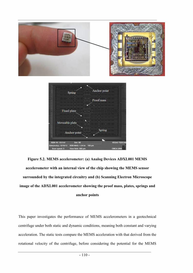
- 110 -
Figure 5.2. MEMS accelerometer: (a) Analog Devices ADXL001 MEMS
accelerometer with an internal view of the chip showing the MEMS sensor
surrounded by the integrated circuitry and (b) Scanning Electron Microscope
image of the ADXL001 accelerometer showing the proof mass, plates, springs and
anchor points
This paper investigates the performance of MEMS accelerometers in a geotechnical
centrifuge under both static and dynamic conditions, meaning both constant and varying
acceleration. The static tests compare the MEMS acceleration with that derived from the
rotational velocity of the centrifuge, before considering the potential for the MEMS
- 111 -
accelerometer to be used as a depth measurement for objects buried in soil. The
dynamic tests focus on embedment of objects free-falling into soil. First, the MEMS
accelerometer is compared with a piezoelectric accelerometer and second the MEMS
accelerometer is used to derive the motion response of an object free-falling through air
and embedding in soil.
5.3. Static centrifuge tests
The MEMS accelerometer performance was first examined under static conditions in
the beam geotechnical centrifuge at The University of Western Australia. In these initial
tests an ADXL001 ±500 g MEMS accelerometer was embedded within an epoxy-filled
void in a strip of aluminium that was rigidly connected to an actuator in an orientation
such that the axis of the MEMS accelerometer was aligned with the direction of the
gravitational field within the centrifuge. The vertical axis
of the actuator was then moved (at 1g) until the radius of the MEMS accelerometer was
equal to the radius at which the nominal g-level was set (1.54 m). A comparison of the
acceleration level measured by the MEMS accelerometer and the acceleration level
calculated using the measured angular velocity of the centrifuge is provided in Figure
5.3a during centrifuge acceleration from 0 to 100 g and back. The only signal
conditioning applied to the signal is a low pass resistor– capacitor (RC) passive filter
with a 3 dB cut-off frequency of 120 kHz and signal averaging in time blocks of 0.1 s.
A slight difference is observed in the measured quantities before and after spinning, as
the MEMS measures Earth‟s gravity and so outputs 1g, whereas the zero angular
velocity infers zero centripetal acceleration. The inset in Figure 5.3a, during which the
acceleration level is a constant 100g, shows good agreement between the acceleration
levels measured by the MEMS accelerometer and derived from the centrifuge‟s
rotational speed. The minimum resolution of the MEMS accelerometer is evident from
- 112 -
the step-ladder response at constant acceleration level. The minimum resolvable
acceleration resolution, ∆N, is given by:
max2N
VVN n
S
ADC 5.1
where VADC is the full scale input voltage range of the ADC (analogue to digital
converter) in the data acquisition system, VS is the full scale output range of the
accelerometer, n is the bit resolution of the ADC and Nmax is the full scale range of the
accelerometer. For these tests where VADC = 10 V, VS = 2.2 V, n = 16 and Nmax = 1000
g (±500 g accelerometer), ∆N is calculated as 0.07 g or 0.69 m/s2. This resolution can be
increased by using a sensor with a lower rated Nmax.
The data in Figure 5.3a are also shown in Figure 5.3b, but with the MEMS sensor
output plotted against the centrifuge acceleration level as the centrifuge acceleration is
increased from 0 to 100 g and back. Figure 5.3b indicates that the response is linear,
although with an apparently slight hysteresis which is attributable to the time delay in
the reporting of the centrifuge rotational speed to the data acquisition system.
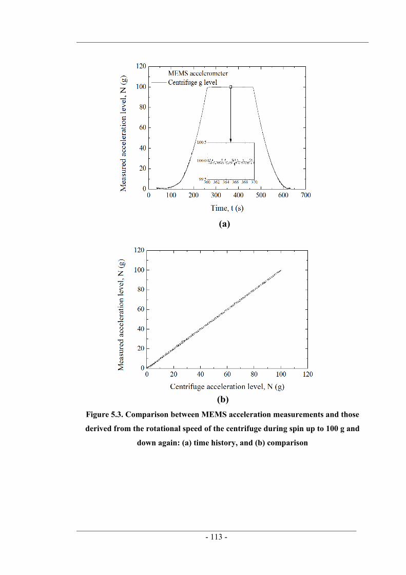
- 113 -
Figure 5.3. Comparison between MEMS acceleration measurements and those
derived from the rotational speed of the centrifuge during spin up to 100 g and
down again: (a) time history, and (b) comparison
(a)
(b)

- 114 -
The vertical axis of the actuator was subsequently moved at 1 mm/s and the radius, R,
derived from the MEMS accelerometer measurements (Equation 5.2) was compared
with the radius established from the vertical displacements of the actuator (measured
using the motor encoder on the vertical axis of the actuator) (Figure 5.4). The agreement
highlights the potential for MEMS accelerometers to be used as a depth indicator in
centrifuge tests. To assess the minimum depth increment that can be detected, the
acceleration level in the centrifuge depends on the radius, R, according to:
by:
RNg 2 5.2
where ω is the angular velocity in rad/s. From Equations 5.1 and 5.2 the minimum
displacement resolution ∆R becomes:
maxmax2 22N
VV
NRN
VVgR n
S
ADCen
S
ADC
5.3
For the tests considered later in the paper, where N = 133.3 at an effective radius, Re =
1.574 m, VADC = 10 V, VS = 2.2 V and Nmax = 1000 g, ∆R is calculated as 0.82 mm.
This resolution will increase as the maximum range of the accelerometer decreases, and
also as the acceleration level in the centrifuge increases. Although this resolution is at
least two orders of magnitude worse than can be achieved using conventional
displacement potentiometers, the small size of the MEMS accelerometer opens up
possibilities for making depth measurements of objects that are buried within a soil
sample, out of reach of a conventional potentiometer. This has particular merit for
freefall penetrometers and dynamically installed anchors, as demonstrated in the
following section.
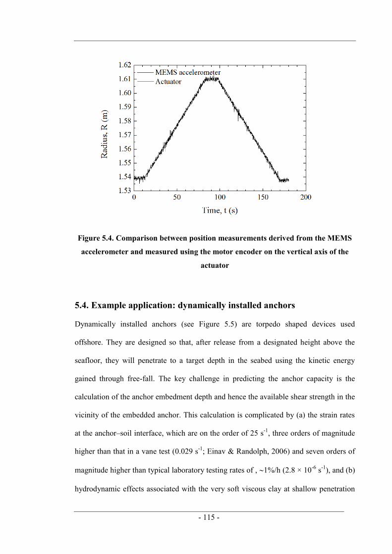
- 115 -
Figure 5.4. Comparison between position measurements derived from the MEMS
accelerometer and measured using the motor encoder on the vertical axis of the
actuator
5.4. Example application: dynamically installed anchors
Dynamically installed anchors (see Figure 5.5) are torpedo shaped devices used
offshore. They are designed so that, after release from a designated height above the
seafloor, they will penetrate to a target depth in the seabed using the kinetic energy
gained through free-fall. The key challenge in predicting the anchor capacity is the
calculation of the anchor embedment depth and hence the available shear strength in the
vicinity of the embedded anchor. This calculation is complicated by (a) the strain rates
at the anchor–soil interface, which are on the order of 25 s-1, three orders of magnitude
higher than that in a vane test (0.029 s-1; Einav & Randolph, 2006) and seven orders of
magnitude higher than typical laboratory testing rates of , 1%/h (2.8 × 10⁻⁶ s-1), and (b)
hydrodynamic effects associated with the very soft viscous clay at shallow penetration
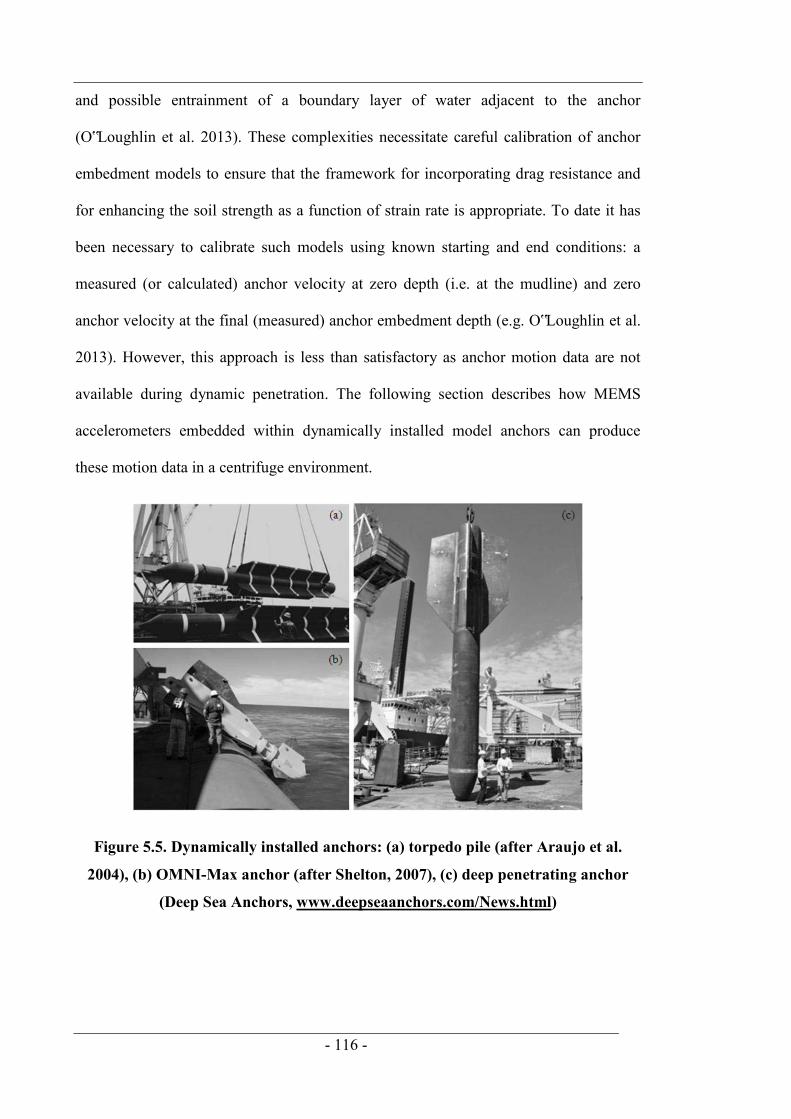
- 116 -
and possible entrainment of a boundary layer of water adjacent to the anchor
(O‟Loughlin et al. 2013). These complexities necessitate careful calibration of anchor
embedment models to ensure that the framework for incorporating drag resistance and
for enhancing the soil strength as a function of strain rate is appropriate. To date it has
been necessary to calibrate such models using known starting and end conditions: a
measured (or calculated) anchor velocity at zero depth (i.e. at the mudline) and zero
anchor velocity at the final (measured) anchor embedment depth (e.g. O‟Loughlin et al.
2013). However, this approach is less than satisfactory as anchor motion data are not
available during dynamic penetration. The following section describes how MEMS
accelerometers embedded within dynamically installed model anchors can produce
these motion data in a centrifuge environment.
Figure 5.5. Dynamically installed anchors: (a) torpedo pile (after Araujo et al.
2004), (b) OMNI-Max anchor (after Shelton, 2007), (c) deep penetrating anchor
(Deep Sea Anchors, www.deepseaanchors.com/News.html)
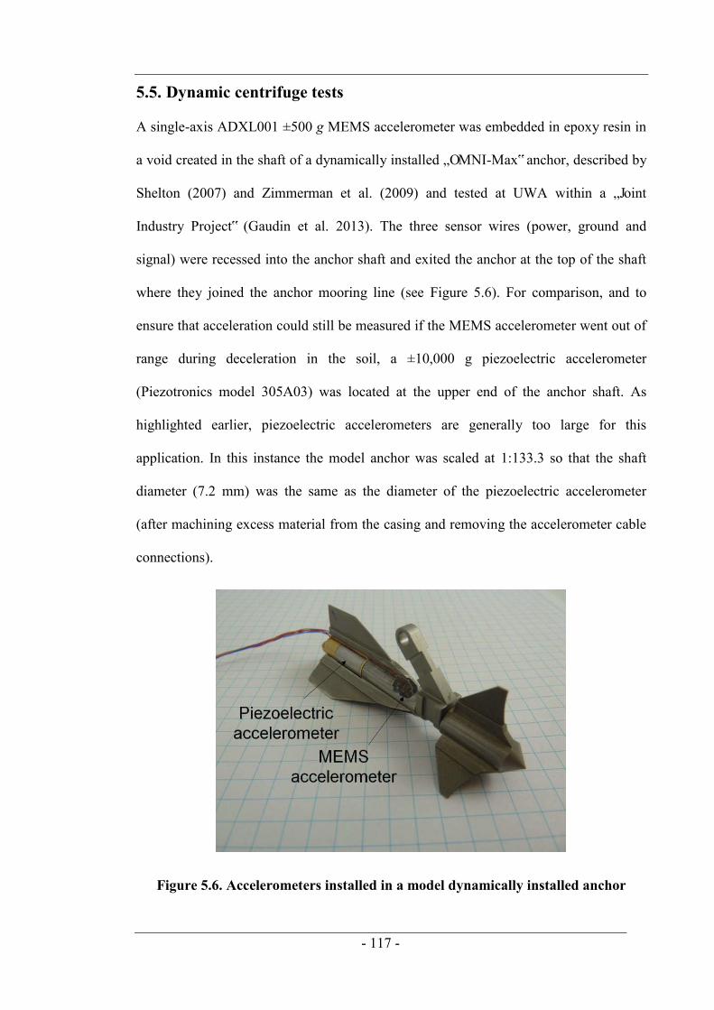
- 117 -
5.5. Dynamic centrifuge tests
A single-axis ADXL001 ±500 g MEMS accelerometer was embedded in epoxy resin in
a void created in the shaft of a dynamically installed „OMNI-Max‟ anchor, described by
Shelton (2007) and Zimmerman et al. (2009) and tested at UWA within a „Joint
Industry Project‟ (Gaudin et al. 2013). The three sensor wires (power, ground and
signal) were recessed into the anchor shaft and exited the anchor at the top of the shaft
where they joined the anchor mooring line (see Figure 5.6). For comparison, and to
ensure that acceleration could still be measured if the MEMS accelerometer went out of
range during deceleration in the soil, a ±10,000 g piezoelectric accelerometer
(Piezotronics model 305A03) was located at the upper end of the anchor shaft. As
highlighted earlier, piezoelectric accelerometers are generally too large for this
application. In this instance the model anchor was scaled at 1:133.3 so that the shaft
diameter (7.2 mm) was the same as the diameter of the piezoelectric accelerometer
(after machining excess material from the casing and removing the accelerometer cable
connections).
Figure 5.6. Accelerometers installed in a model dynamically installed anchor
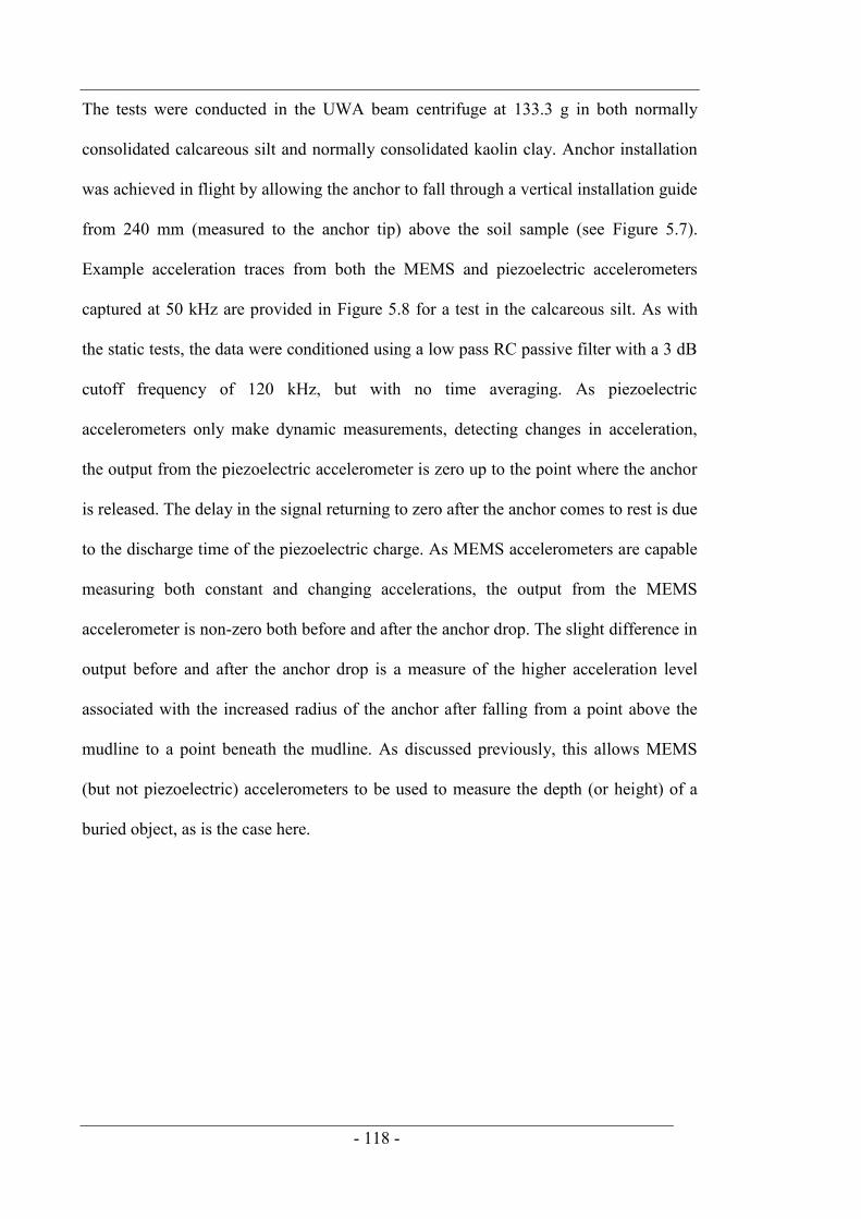
- 118 -
The tests were conducted in the UWA beam centrifuge at 133.3 g in both normally
consolidated calcareous silt and normally consolidated kaolin clay. Anchor installation
was achieved in flight by allowing the anchor to fall through a vertical installation guide
from 240 mm (measured to the anchor tip) above the soil sample (see Figure 5.7).
Example acceleration traces from both the MEMS and piezoelectric accelerometers
captured at 50 kHz are provided in Figure 5.8 for a test in the calcareous silt. As with
the static tests, the data were conditioned using a low pass RC passive filter with a 3 dB
cutoff frequency of 120 kHz, but with no time averaging. As piezoelectric
accelerometers only make dynamic measurements, detecting changes in acceleration,
the output from the piezoelectric accelerometer is zero up to the point where the anchor
is released. The delay in the signal returning to zero after the anchor comes to rest is due
to the discharge time of the piezoelectric charge. As MEMS accelerometers are capable
measuring both constant and changing accelerations, the output from the MEMS
accelerometer is non-zero both before and after the anchor drop. The slight difference in
output before and after the anchor drop is a measure of the higher acceleration level
associated with the increased radius of the anchor after falling from a point above the
mudline to a point beneath the mudline. As discussed previously, this allows MEMS
(but not piezoelectric) accelerometers to be used to measure the depth (or height) of a
buried object, as is the case here.

- 119 -
Figure 5.7. Dynamic anchor experimental arrangement showing the anchor
located in installation guide before release and embedded in the soil sample after
release
Anchor in soilSample
Water
Anchor in soilSample
Water
Anchor in guide
Mooring line
Anchor release mechanism
Mooring line
Anchor installation guide
Side view End view
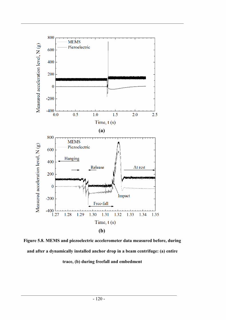
- 120 -
Figure 5.8. MEMS and piezoelectric accelerometer data measured before, during
and after a dynamically installed anchor drop in a beam centrifuge: (a) entire
trace, (b) during freefall and embedment
(a)
(b)
- 121 -
Accelerations measured during the test are shown more clearly on Figure 5.8b, in which
the time scale has been clipped to show the anchor release and embedment in more
detail. The electrical noise on the MEMS accelerometer signal is approximately ±15 g,
compared with ±2.5 g on the piezoelectric accelerometer signal. As a ratio of the full
range output, the noise level of the MEMS accelerometer is approximately 100 times
higher than the piezoelectric accelerometer. The higher noise for the MEMS
accelerometer is well-known (e.g. Ratcliffe et al. 2008), and is higher in these dynamic
tests as no time averaging was applied to the data sampled by the ADC. However, the
±15 g noise level on the MEMS accelerometer is not considered to be problematic as
the data are eventually integrated to obtain velocities and displacements, effectively
averaging the noise error.
The saw tooth response at the beginning of the drop is a consequence of the anchor
release method. This was achieved inflight using a resistor which, when supplied with
current, heated and subsequently burned through a sacrificial anchor release cord. The
cord consists of multiple strands which likely parted sequentially, causing the changes
in acceleration over the first couple of milliseconds of the drop. During free-fall, the
MEMS accelerometer outputs approximately zero acceleration as expected, since there
is no force acting on the anchor except for a small component of Earth‟s gravity. This
acts at an inclination of tan-1(120) to the anchor giving a component of 0.01 g.
The piezoelectric accelerometer initially responds with the correct change in
acceleration of ,120g (i.e. the centrifuge acceleration level at the radius of the anchor
release location), but then starts to discharge towards zero as the acceleration during
free-fall is essentially constant and zero. This precludes the piezoelectric accelerometer
from being used as a means of establishing the free-fall velocity profile and hence the
anchor‟s velocity at the mudline.

- 122 -
5.6. Interpretation of accelerometer data
Numerical integration of acceleration yields velocity (after a single integration) and
displacement (after double integration), allowing a depth profile of acceleration and
velocity to be established for the anchor as it penetrates the soil. The integration is
undertaken within the rotating frame of reference, such that it is the anchor acceleration,
velocity and displacement relative to the soil surface that is considered.
As the precise release point can be difficult to identify (see Figure 5.8), the most
appropriate starting point for the numerical integration is when the anchor is stationary
relative to the soil at zero (relative) velocity and at a measured embedment depth. In this
test, the final anchor embedment depth was measured at 1g by clamping the release cord
trailing from the anchor at the soil surface, extracting the anchor, and then measuring
the distance from the clamp location to the anchor tip.
The integration is performed in reverse from the end of the test when the anchor is at
rest in the soil and so the relative acceleration is zero and the centrifuge (and hence
anchor) acceleration and radius is given by the MEMS accelerometer measurements.
The anchor acceleration relative to the soil during embedment and free-fall can then be
calculated using Equation 5.2, where the updated radius is determined from the at-rest
radius and the change in embedment calculated from the integration. The MEMS
acceleration data in Figure 5.8 are replotted in Figure 5.9a together with the centrifuge
(and soil) acceleration associated with the current anchor location during freefall and
embedment, and the anchor velocity and displacement relative to the soil.
The anchor velocity relative to the soil increases during free-fall due to the centrifuge
acceleration of the soil. At time t = 1.316 s the impact with the soil occurs which
corresponds to a peak anchor velocity, v = 22 m/s and an anchor displacement, ∆z =
80.4 mm (measured up from the at rest position). The directly measured anchor tip
- 123 -
embedment depth was 80.5 mm, which implies that the anchor reached its maximum
velocity and began to decelerate as soon as it impacted the soil surface. The anchor
comes to rest in the soil at t = 1.323 s before rebounding slightly. This effect is most
evident on the acceleration trace, with the numerical integration producing a lessening
effect on the velocity and displacement. This rebound has been reported in other studies
involving free-fall objects (e.g. Chow & Airey, 2010; Dayal & Allen, 1973; Morton &
O‟Loughlin, 2012), and is attributed to elastic rebound of the soil.
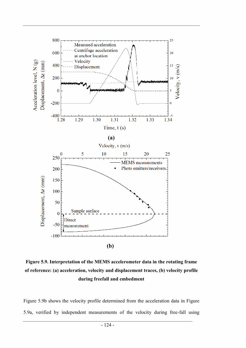
- 124 -
Figure 5.9. Interpretation of the MEMS accelerometer data in the rotating frame
of reference: (a) acceleration, velocity and displacement traces, (b) velocity profile
during freefall and embedment
Figure 5.9b shows the velocity profile determined from the acceleration data in Figure
5.9a, verified by independent measurements of the velocity during free-fall using
(a)
(b)
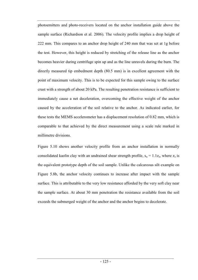
- 125 -
photoemitters and photo-receivers located on the anchor installation guide above the
sample surface (Richardson et al. 2006). The velocity profile implies a drop height of
222 mm. This compares to an anchor drop height of 240 mm that was set at 1g before
the test. However, this height is reduced by stretching of the release line as the anchor
becomes heavier during centrifuge spin up and as the line unravels during the burn. The
directly measured tip embedment depth (80.5 mm) is in excellent agreement with the
point of maximum velocity. This is to be expected for this sample owing to the surface
crust with a strength of about 20 kPa. The resulting penetration resistance is sufficient to
immediately cause a net deceleration, overcoming the effective weight of the anchor
caused by the acceleration of the soil relative to the anchor. As indicated earlier, for
these tests the MEMS accelerometer has a displacement resolution of 0.82 mm, which is
comparable to that achieved by the direct measurement using a scale rule marked in
millimetre divisions.
Figure 5.10 shows another velocity profile from an anchor installation in normally
consolidated kaolin clay with an undrained shear strength profile, su = 1.1zs, where zs is
the equivalent prototype depth of the soil sample. Unlike the calcareous silt example on
Figure 5.8b, the anchor velocity continues to increase after impact with the sample
surface. This is attributable to the very low resistance afforded by the very soft clay near
the sample surface. At about 30 mm penetration the resistance available from the soil
exceeds the submerged weight of the anchor and the anchor begins to decelerate.

- 126 -
Figure 5.10. Anchor velocity profiles for an anchor installation in kaolin clay with
su = 1.1z
As shown by Figure 5.7, in these experiments the vertical installation guide located
above the centreline of the soil sample prevents the anchor tilting during the freefall
stage, and applies the tangential force needed to keep the anchor rotating at the same
angular velocity as the centrifuge, which requires an increasing tangential velocity with
increasing radius. Once the anchor is embedded in the soil, this force must be applied by
the soil and there may be a tendency for the anchor to follow a curved trajectory through
the sample. This effect could be more significant when the soil is softer, such as in the
kaolin clay test (where the tip embedment was 2.5 times the anchor length compared
with 1.2 times the anchor length for the calcareous silt test) as the curved path is more
likely if the soil does not provide the resistance needed to accelerate the anchor
tangentially.

- 127 -
If the anchor tilts, the sensing axis of the MEMS accelerometer will not be coincident
with the centripetal acceleration vector, and the resulting acceleration measurements
will be lower than the centrifuge acceleration. The influence of tilt during anchor
embedment in soil is explored further in Figure 5.11, where various tilt angles are
artificially introduced to the MEMS acceleration trace measured in the kaolin clay test
at an anchor tip embedment of one anchor length. As the integration starts in reverse
from the at-rest position, the effect of tilt (applied to the acceleration trace only when
the anchor is free of the guide) has a cumulative effect all the way to the release point.
Figure 5.11 shows that tilt angles up to 10˚ have negligible effect on the velocity profile,
with a maximum reduction in impact velocity and final embedment depth of 1.4% and
1% respectively. However, for a tilt angle of 20˚ the reduction increases to 5.4% on
impact velocity and 3.7% on final embedment depth, and for a tilt angle of 30˚ impact
velocity reduces by 11.8% and final embedment depth reduces by 8.1%. Although the
final tilt angle can be quantified by using a dual or tri-axis accelerometer, the agreement
between the MEMS measurements and those made independently indicates that the
anchor tilt angle was negligible in the tests considered here.
Commercially available MEMS accelerometers are generally limited to a maximum
rated acceleration level of ±500 g. As such the sensor signal can become saturated
during impact events at higher centrifuge acceleration levels or for samples with higher
strengths. Figure 5.9a shows MEMS acceleration levels that are above the 500 g
maximum rated range of the sensor, which will have an effect on the linearity of the
sensor output at these „excess‟ acceleration levels. These two limitations need to be
considered in the experimental design.
- 128 -
(a)
(b)

- 129 -
Figure 5.11. Effect of anchor tilt during embedment in soil (kaolin clay with su =
1.1z): (a) 5 degree tilt, (b) 10 degree tilt, (c) 20 degree tilt, (d) 30 degree tilt
(c)
(d)

- 130 -
5.7. Concluding remarks
MEMS accelerometers are small, inexpensive sensors that have rarely been used in
geotechnical centrifuge modelling despite widespread use in consumer devices and for
industrial applications. Unlike piezoelectric accelerometers, MEMS accelerometers
measure both constant and varying acceleration. This feature has been exploited in the
paper to measure the motion response of a dynamically installed anchor as it free-falls
through air and embeds within a centrifuge soil sample. The capability of the MEMs
device to detect constant acceleration levels allows the centrifuge acceleration
component, and its variation with radial position, also to be detected. The motion
response can be used to produce acceleration or velocity depth profiles for the anchor;
such profiles are important for the calibration and validation of embedment prediction
tools for dynamically installed anchors.
- 131 -
CHAPTER 6. IN-SITU MEASUREMENT OF THE
DYNAMIC PENETRATION OF FREE FALL
PROJECTLES IN SOFT SOILS USING A LOW COST
INERTIAL MEASUREMENT UNIT
6.1. Abstract
Six degree-of-freedom motion data from projectiles free-falling through water and
embedding in soft soil are measured using a low-cost inertial measurement unit,
consisting of a tri-axis accelerometer and a three-component gyroscope. A
comprehensive framework for interpreting the measured data is described and the merit
of this framework is demonstrated by considering sample test data for free-falling
projectiles that gain velocity as they fall through water and self-embed in the underlying
This chapter describes a novel theoretical framework for interpretation of in situ IMU
data. This framework is then used in Chapter 7 in the analysis of the IFFS test data
and a reduced, simplified form of the framework is used in the analysis of the IFFS
centrifuge data.
Blake, A. P., O'Loughlin, C. D., Morton, J. P., O' Beirne, C., Gaudin, C. & White, D.
J., 2015. In-situ measurement of the dynamic penetration of freefall projectiles in soft
soils using a low cost inertial measurement unit. Geotechnical Testing Journal,
ASTM. DOI: 10.1520/GTJ20140135.

- 132 -
soft clay. The paper shows the importance of considering such motion data from an
appropriate reference frame by showing good agreement in embedment depth data
derived from the motion data with independent direct measurements. Motion data
derived from the inertial measurement unit are used to calibrate a predictive model for
calculating the final embedment depth of a dynamically installed anchor.
6.2. Introduction
An inertial measurement unit (IMU) is an electromechanical device that measures an
object‟s six degree of freedom (6DoF) motion in three-dimensional space using a
combination of gyroscope and accelerometer sensors. The development of micro-electro
mechanical systems (MEMS) gyroscope and accelerometer technology has significantly
reduced the cost, size, weight and power consumption of IMUs, and enhanced their
robustness.
MEMS accelerometers and gyroscopes are typically fabricated on single-crystal silicon
wafers using micromachining to etch defined patterns on a silicon substrate. These
patterns take the form of small proof masses that are free from the substrate and
surrounded by fixed plates. The proof mass is connected to a fixed frame by flexible
beams, effectively forming spring elements. Low-cost consumer grade MEMS
gyroscopes typically use vibrating mechanical elements to sense angular rotation rate.
During operation the proof mass is resonated with constant amplitude in the „drive
direction‟ by an external sinusoidal electrostatic or electromagnetic force. Angular
rotation then induces a matched-frequency sinusoidal Coriolis force orthogonal to the
drive-mode oscillation and the axis of rotation. The Coriolis force deflects the proof
mass and plates connected to the proof mass move between the fixed plates in the sense-
mode. The operational principle for MEMS accelerometers is much simpler;
accelerations acting on the proof mass cause it to displace, and plates connected to the
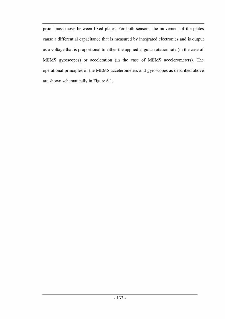
- 133 -
proof mass move between fixed plates. For both sensors, the movement of the plates
cause a differential capacitance that is measured by integrated electronics and is output
as a voltage that is proportional to either the applied angular rotation rate (in the case of
MEMS gyroscopes) or acceleration (in the case of MEMS accelerometers). The
operational principles of the MEMS accelerometers and gyroscopes as described above
are shown schematically in Figure 6.1.
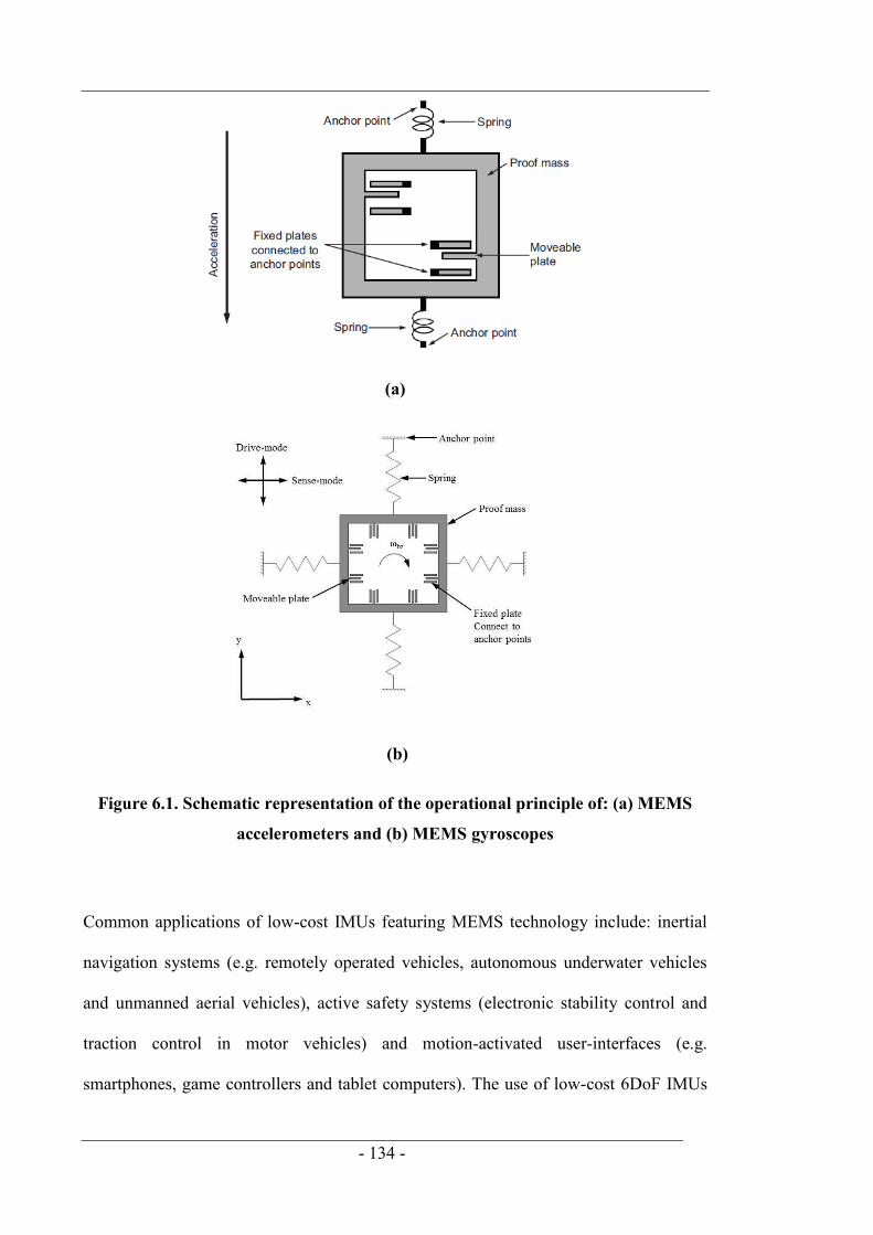
- 134 -
(a)
(b)
Figure 6.1. Schematic representation of the operational principle of: (a) MEMS
accelerometers and (b) MEMS gyroscopes
Common applications of low-cost IMUs featuring MEMS technology include: inertial
navigation systems (e.g. remotely operated vehicles, autonomous underwater vehicles
and unmanned aerial vehicles), active safety systems (electronic stability control and
traction control in motor vehicles) and motion-activated user-interfaces (e.g.
smartphones, game controllers and tablet computers). The use of low-cost 6DoF IMUs

- 135 -
for geotechnical applications has not been reported. However, MEMS accelerometers
have been used for in situ geotechnical applications to measure: inclinations in
boreholes (Bennett et al. 2009), soil displacement associated with rapid uplift of
footings (Levy & Richards 2012) and the motion of free-falling cone penetrometers
(e.g. Stegmann et al. 2006; Stephan et al. 2012; Steiner et al. 2014). In geotechnical
centrifuge modelling MEMS accelerometers have been used to measure: the
acceleration response of free-falling projectiles in clay (O‟Loughlin et al. 2014; Chow et
al. 2014), earthquake accelerations (Cilingir & Madabhushi 2011; Stringer et al. 2010)
and rotation of structures during slow lateral cycling and dynamic shaking (Allmond et
al. 2014). Although accelerometers are often used to measure the rotation of objects at
constant acceleration, they cannot distinguish rotation from linear acceleration if the
object‟s orientation and acceleration is changing. However, gyroscopes are unaffected
by linear acceleration, and the rotation of accelerating objects can be derived from their
measurements. Hence the combination of accelerometer and gyroscope measurements
enables an object‟s linear acceleration to be determined relative to a reference frame
that is not necessarily coincident with the reference frame of the object. This becomes
important for the applications considered in this paper, where dynamically installed
anchors and a free-falling sphere (collectively referred to as „projectiles‟ from this point
forward) free fall through water and bury in the underlying soil. As described later, the
motion response of the projectile must be considered from the appropriate reference
frame. From the viewpoint of the hydrodynamic and geotechnical resistances acting on
the projectile during motion, it becomes important to consider the projectile‟s trajectory,
whereas from a geotechnical design viewpoint the final depth and orientation of the
projectile relative to a fixed inertial frame of reference (with an axis in the direction of
Earth‟s gravity) is important as this will dictate the local soil strength in the vicinity of
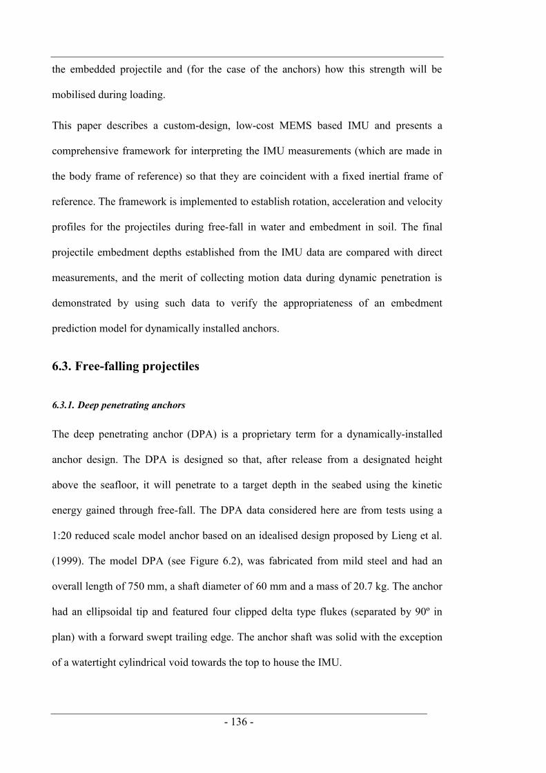
- 136 -
the embedded projectile and (for the case of the anchors) how this strength will be
mobilised during loading.
This paper describes a custom-design, low-cost MEMS based IMU and presents a
comprehensive framework for interpreting the IMU measurements (which are made in
the body frame of reference) so that they are coincident with a fixed inertial frame of
reference. The framework is implemented to establish rotation, acceleration and velocity
profiles for the projectiles during free-fall in water and embedment in soil. The final
projectile embedment depths established from the IMU data are compared with direct
measurements, and the merit of collecting motion data during dynamic penetration is
demonstrated by using such data to verify the appropriateness of an embedment
prediction model for dynamically installed anchors.
6.3. Free-falling projectiles
6.3.1. Deep penetrating anchors
The deep penetrating anchor (DPA) is a proprietary term for a dynamically-installed
anchor design. The DPA is designed so that, after release from a designated height
above the seafloor, it will penetrate to a target depth in the seabed using the kinetic
energy gained through free-fall. The DPA data considered here are from tests using a
1:20 reduced scale model anchor based on an idealised design proposed by Lieng et al.
(1999). The model DPA (see Figure 6.2), was fabricated from mild steel and had an
overall length of 750 mm, a shaft diameter of 60 mm and a mass of 20.7 kg. The anchor
had an ellipsoidal tip and featured four clipped delta type flukes (separated by 90º in
plan) with a forward swept trailing edge. The anchor shaft was solid with the exception
of a watertight cylindrical void towards the top to house the IMU.

- 137 -
Figure 6.2. Deep penetrating anchor
6.3.2. Dynamically embedded plate anchors
The dynamically embedded plate anchor (DEPLA, O‟Loughlin et al. 2013a) is an
anchoring system that combines the capacity advantages of vertically loaded anchors
with the installation advantages of dynamically installed anchors. The DEPLA
comprises a removable central shaft or „follower‟ and a set of four flukes (see Figure
6.3). A stop cap at the upper end of the follower prevents it from falling through the
DEPLA sleeve and a shear pin connects the flukes to the follower. The DEPLA is
installed in a similar manner as the DPA, but after coming to rest in the seabed the
follower retriever line is tensioned, which causes the shear pin to part (if not already
broken during impact) allowing the follower to be retrieved for the next installation
whilst leaving the anchor flukes vertically embedded in the seabed. These embedded
anchor flukes constitute the load bearing element as a plate anchor.
In the tests considered here the DEPLA was modelled at a reduced scale of 1:4.5 and
fabricated from mild steel. The follower (and hence DEPLA) length was 2 m, the
follower diameter was 160 mm, the fluke (plate) diameter was 800 mm and the overall
mass was 388.6 kg. As with the DPA, the DEPLA follower was solid with the exception
of a cylindrical void at the top to house the IMU. The model DEPLA is shown in Figure
6.3.
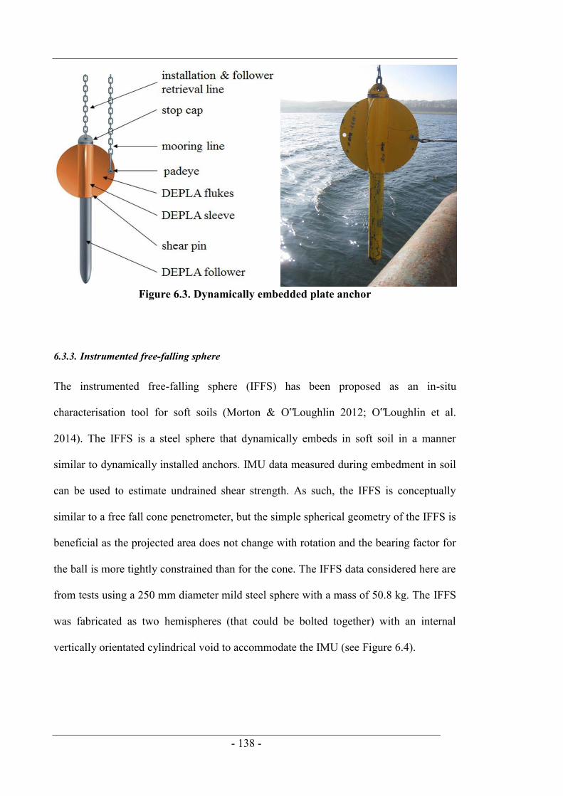
- 138 -
Figure 6.3. Dynamically embedded plate anchor
6.3.3. Instrumented free-falling sphere
The instrumented free-falling sphere (IFFS) has been proposed as an in-situ
characterisation tool for soft soils (Morton & O‟Loughlin 2012; O‟Loughlin et al.
2014). The IFFS is a steel sphere that dynamically embeds in soft soil in a manner
similar to dynamically installed anchors. IMU data measured during embedment in soil
can be used to estimate undrained shear strength. As such, the IFFS is conceptually
similar to a free fall cone penetrometer, but the simple spherical geometry of the IFFS is
beneficial as the projected area does not change with rotation and the bearing factor for
the ball is more tightly constrained than for the cone. The IFFS data considered here are
from tests using a 250 mm diameter mild steel sphere with a mass of 50.8 kg. The IFFS
was fabricated as two hemispheres (that could be bolted together) with an internal
vertically orientated cylindrical void to accommodate the IMU (see Figure 6.4).
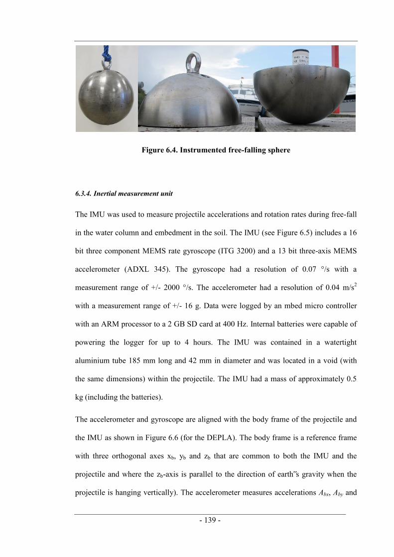
- 139 -
Figure 6.4. Instrumented free-falling sphere
6.3.4. Inertial measurement unit
The IMU was used to measure projectile accelerations and rotation rates during free-fall
in the water column and embedment in the soil. The IMU (see Figure 6.5) includes a 16
bit three component MEMS rate gyroscope (ITG 3200) and a 13 bit three-axis MEMS
accelerometer (ADXL 345). The gyroscope had a resolution of 0.07 °/s with a
measurement range of +/- 2000 °/s. The accelerometer had a resolution of 0.04 m/s2
with a measurement range of +/- 16 g. Data were logged by an mbed micro controller
with an ARM processor to a 2 GB SD card at 400 Hz. Internal batteries were capable of
powering the logger for up to 4 hours. The IMU was contained in a watertight
aluminium tube 185 mm long and 42 mm in diameter and was located in a void (with
the same dimensions) within the projectile. The IMU had a mass of approximately 0.5
kg (including the batteries).
The accelerometer and gyroscope are aligned with the body frame of the projectile and
the IMU as shown in Figure 6.6 (for the DEPLA). The body frame is a reference frame
with three orthogonal axes xb, yb and zb that are common to both the IMU and the
projectile and where the zb-axis is parallel to the direction of earth‟s gravity when the
projectile is hanging vertically). The accelerometer measures accelerations Abx, Aby and

- 140 -
Abz in the body frame along these three axes. These accelerometer measurements
include a component of gravitational acceleration (depending on the orientation of the
accelerometer) and linear acceleration. The gyroscope measures angular velocities ωbx,
ωby and ωbz in the body frame about the same orthogonal axes. Accelerometers are often
used to measure the rotation of quasi-static objects but cannot distinguish rotation from
linear acceleration if an object is in motion. However, gyroscopes are unaffected by
linear acceleration and the rotation of objects in motion can be derived from their
measurements.
Figure 6.5. Inertial Measurement Unit
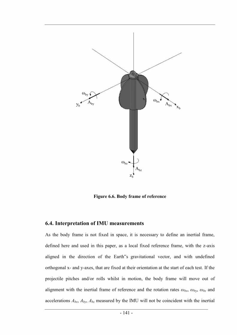
- 141 -
Figure 6.6. Body frame of reference
6.4. Interpretation of IMU measurements
As the body frame is not fixed in space, it is necessary to define an inertial frame,
defined here and used in this paper, as a local fixed reference frame, with the z-axis
aligned in the direction of the Earth‟s gravitational vector, and with undefined
orthogonal x- and y-axes, that are fixed at their orientation at the start of each test. If the
projectile pitches and/or rolls whilst in motion, the body frame will move out of
alignment with the inertial frame of reference and the rotation rates ωbx, ωby, ωbz and
accelerations Abx, Aby, Abz measured by the IMU will not be coincident with the inertial
ωby
ωbx
ωbz
yb xb
zb
Aby Abx
Abz

- 142 -
frame (see Figure 6.7). As a consequence gravitational acceleration g, and linear
acceleration a (required for velocity and translation calculations as described later),
components cannot be distinguished from the accelerometer measurements. Hence the
IMU measurements were „transformed‟ from the body frame to the inertial frame. This
was accomplished using transformation matrices as described in the following sections.
Figure 6.7. Resultant tilt angle, μ, defined in the inertial frame
6.4.1. Rotation
The body frame rotation rates ωbx, ωby, ωbz were transformed from the body frame to the
inertial frame to correspond with rotation rates about the inertial frame ωx, ωy, ωz using
an angular velocity transformation matrix (AVTM), ibT (Fossen 2011):
bz
by
bxi
b
z
y
x
T
6.1
y
zb
μ
z
x
xb
yb
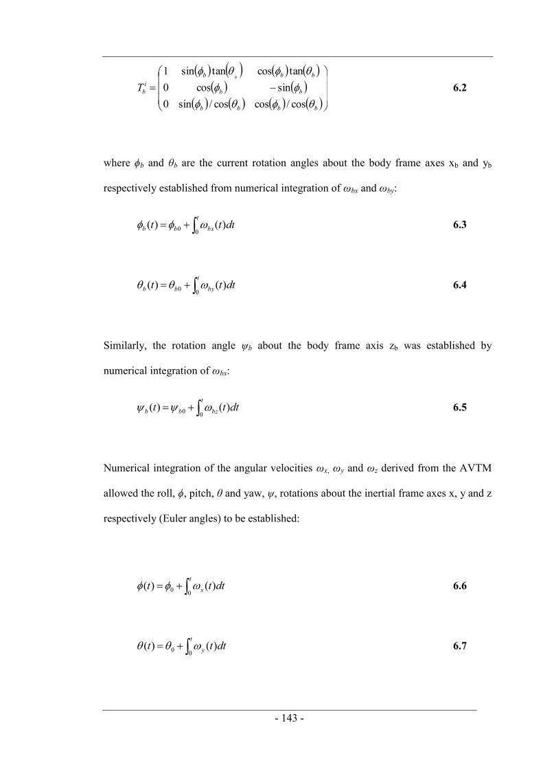
- 143 -
bbbb
bb
bbbi
b
b
T
cos/coscos/sin0sincos0
tancostansin1 6.2
where ϕb and θb are the current rotation angles about the body frame axes xb and yb
respectively established from numerical integration of ωbx and ωby:
t
bxbb dttt00 )()( 6.3
t
bybb dttt00 )()( 6.4
Similarly, the rotation angle ψb about the body frame axis zb was established by
numerical integration of ωbx:
t
bzbb dttt00 )()( 6.5
Numerical integration of the angular velocities ωx, ωy and ωz derived from the AVTM
allowed the roll, ϕ, pitch, θ and yaw, ψ, rotations about the inertial frame axes x, y and z
respectively (Euler angles) to be established:
t
x dttt00 )()( 6.6
t
y dttt00 )()( 6.7

- 144 -
t
z dttt00 )()( 6.8
6.4.2. Acceleration
The accelerometer measurements Abx, Aby and Abz were converted to accelerations
coincident with the inertial frame Ax, Ay and Az using a direction cosine matrix (DCM)
ibR (Nebot & Durrant-Whyte 1999; Jonkman 2007; King et al. 2008; Fossen 2011):
bz
by
bxib
z
y
x
AAA
RAAA
6.9
xyzib RRRR 6.10
The DCM relates the accelerations measured in the body frame to the inertial frame by
considering three successive rotations of yaw -ψ, pitch -θ, and roll -ϕ, about the inertial
frame axes z, y and x respectively. These rotations are represented by the yaw Rz(-ψ),
pitch Ry(-θ) and roll Rx(-ϕ), matrices that are used to rotate the measured acceleration
vectors Abx, Aby and Abz in Euclidean vector space:
1000cossin0sincos
zR 6.11
cos0sin010
sin0cos
yR 6.12
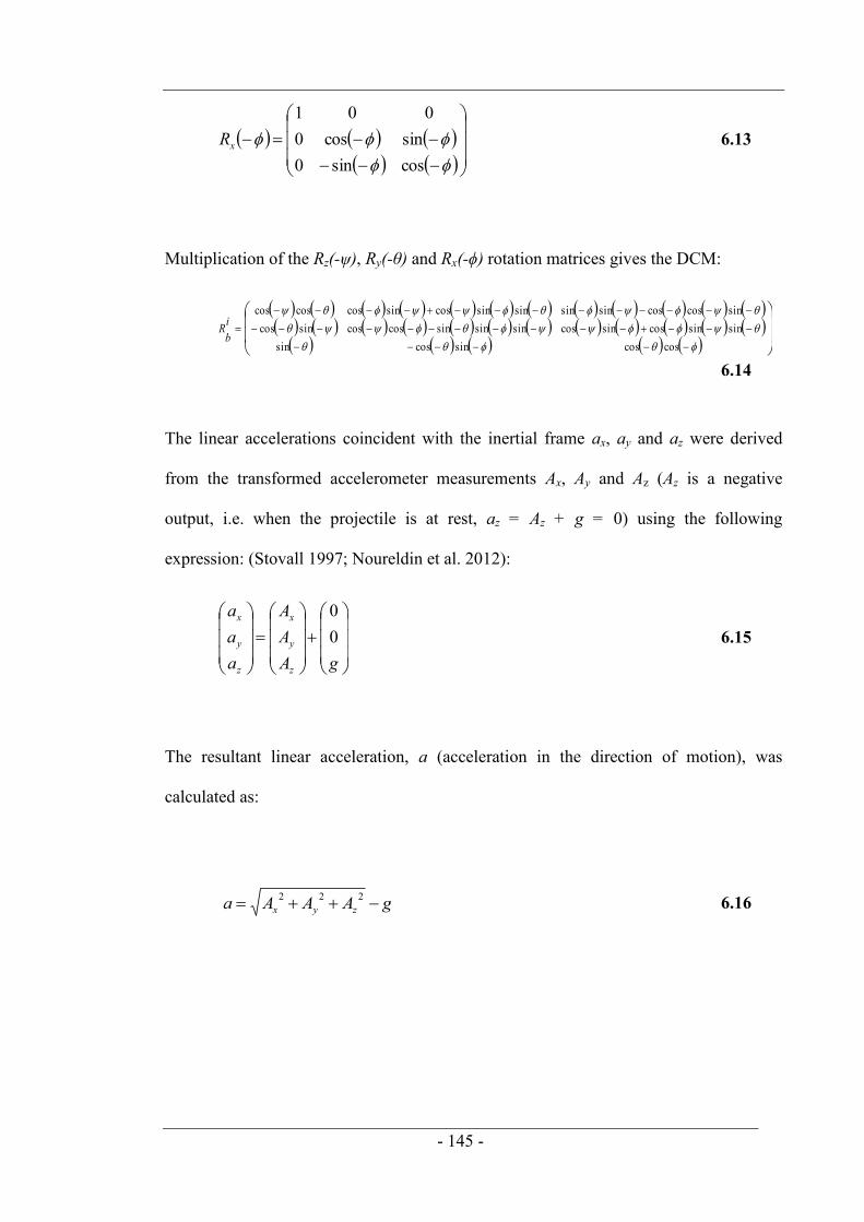
- 145 -
cossin0sincos0
001
xR 6.13
Multiplication of the Rz(-ψ), Ry(-θ) and Rx(-ϕ) rotation matrices gives the DCM:
coscossincossinsinsincossincossinsinsincoscossincossincoscossinsinsinsincossincoscoscos
ib
R
6.14
The linear accelerations coincident with the inertial frame ax, ay and az were derived
from the transformed accelerometer measurements Ax, Ay and Az (Az is a negative
output, i.e. when the projectile is at rest, az = Az + g = 0) using the following
expression: (Stovall 1997; Noureldin et al. 2012):
gAAA
aaa
z
y
x
z
y
x
00
6.15
The resultant linear acceleration, a (acceleration in the direction of motion), was
calculated as:
gAAAa zyx 222 6.16

- 146 -
6.4.3. Velocity and distance
The linear accelerations corresponding to the inertial frame ax, ay and az were
numerically integrated to establish the projectile velocities coincident with the inertial
frame vx, vy and vz during free-fall in the water column and embedment in the soil:
t
xxx dttavtv00 )()( 6.17
t
yyy dttavtv00
)()( 6.18
t
zzz dttavtv00 )()( 6.19
The resultant projectile velocity v, was calculated using the following expression:
222zyx vvvv 6.20
The resultant projectile velocity v, was numerically integrated to establish the distance
travelled by the projectile along its trajectory s:
t
dttvsts00 )()( 6.21
The distance travelled by the projectile along the inertial z axis sz (required to calculate
the vertical embedment depth of the projectile relative to the soil surface, ze), was
established by numerically integrating the vertical velocity vz:
t
zzz dttvsts00 )()( 6.22

- 147 -
6.4.4. Tilt angles
Following dynamic penetration the projectile is at rest in the soil and has no linear
acceleration. Under these conditions the accelerometer measurements can be used to
derive the final pitch ϕacc, roll θacc, (coincident with the inertial frame) and resultant tilt
μ, (tilt relative to Earth‟s gravitational vector, see Figure 6.7) angles using the following
expressions:
gAby
acc1sin (King et al. 2008) 6.23
gAbx
acc1sin (King et al. 2008) 6.24
gAbz1cos (Stephan et al. 2012) 6.25
6.5. Test sites and soil properties
The IMU performance has been examined using projectile data from two sites. The
DEPLA data considered here relate to tests conducted in the Firth of Clyde which is
located off the West coast of Scotland between the mainland and the Isle of Cumbrae.
The DPA and IFFS data are from tests conducted in Lower Lough Erne, which is an
inland lake located in County Fermanagh, Northern Ireland. At Lough Erne the water
depths at the test locations varied between 3 and 20 m whereas at the Firth of Clyde test
locations the water depth was typically 50 m. Both test locations are shown in Figure
6.8.
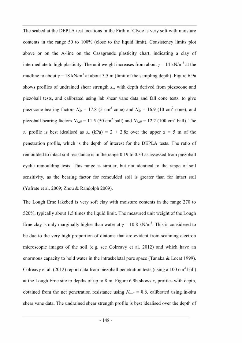
- 148 -
The seabed at the DEPLA test locations in the Firth of Clyde is very soft with moisture
contents in the range 50 to 100% (close to the liquid limit). Consistency limits plot
above or on the A-line on the Casagrande plasticity chart, indicating a clay of
intermediate to high plasticity. The unit weight increases from about γ = 14 kN/m3 at the
mudline to about γ = 18 kN/m3 at about 3.5 m (limit of the sampling depth). Figure 6.9a
shows profiles of undrained shear strength su, with depth derived from piezocone and
piezoball tests, and calibrated using lab shear vane data and fall cone tests, to give
piezocone bearing factors Nkt = 17.8 (5 cm2 cone) and Nkt = 16.9 (10 cm2 cone), and
piezoball bearing factors Nball = 11.5 (50 cm2 ball) and Nball = 12.2 (100 cm2 ball). The
su profile is best idealised as su (kPa) = 2 + 2.8z over the upper z = 5 m of the
penetration profile, which is the depth of interest for the DEPLA tests. The ratio of
remoulded to intact soil resistance is in the range 0.19 to 0.33 as assessed from piezoball
cyclic remoulding tests. This range is similar, but not identical to the range of soil
sensitivity, as the bearing factor for remoulded soil is greater than for intact soil
(Yafrate et al. 2009; Zhou & Randolph 2009).
The Lough Erne lakebed is very soft clay with moisture contents in the range 270 to
520%, typically about 1.5 times the liquid limit. The measured unit weight of the Lough
Erne clay is only marginally higher than water at γ = 10.8 kN/m3. This is considered to
be due to the very high proportion of diatoms that are evident from scanning electron
microscopic images of the soil (e.g. see Colreavy et al. 2012) and which have an
enormous capacity to hold water in the intraskeletal pore space (Tanaka & Locat 1999).
Colreavy et al. (2012) report data from piezoball penetration tests (using a 100 cm2 ball)
at the Lough Erne site to depths of up to 8 m. Figure 6.9b shows su profiles with depth,
obtained from the net penetration resistance using Nball = 8.6, calibrated using in-situ
shear vane data. The undrained shear strength profile is best idealised over the depth of

- 149 -
interest (0 to 2.2 m) as su (kPa) = 1.5z. Piezoball cyclic remoulding tests show that the
ratio of remoulded to intact soil resistance is in the narrow range 0.4 to 0.5, indicating a
low sensitivity soil.
Figure 6.8. Test sites locations
Lough Erne
Firth of Clyde
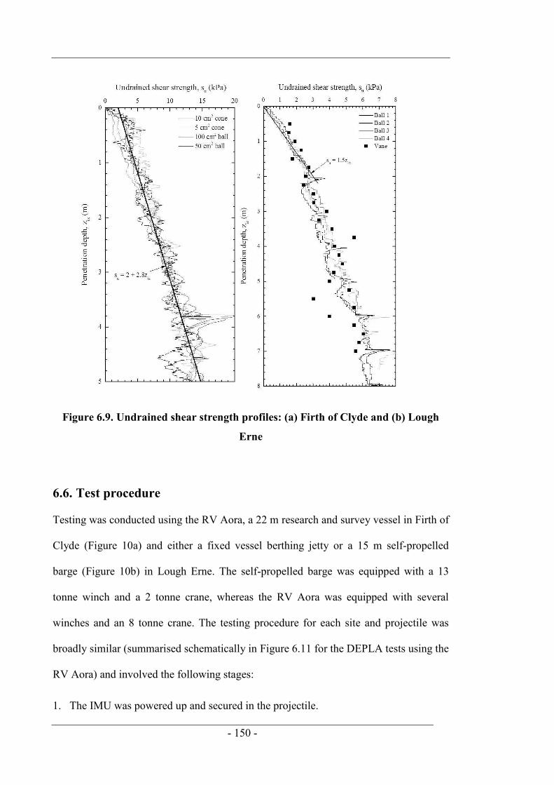
- 150 -
Figure 6.9. Undrained shear strength profiles: (a) Firth of Clyde and (b) Lough
Erne
6.6. Test procedure
Testing was conducted using the RV Aora, a 22 m research and survey vessel in Firth of
Clyde (Figure 10a) and either a fixed vessel berthing jetty or a 15 m self-propelled
barge (Figure 10b) in Lough Erne. The self-propelled barge was equipped with a 13
tonne winch and a 2 tonne crane, whereas the RV Aora was equipped with several
winches and an 8 tonne crane. The testing procedure for each site and projectile was
broadly similar (summarised schematically in Figure 6.11 for the DEPLA tests using the
RV Aora) and involved the following stages:
1. The IMU was powered up and secured in the projectile.

- 151 -
2. The projectile was lowered below the water surface to the desired drop height above
the mudline.
3. The projectile was released by opening a quick release shackle connecting the
projectile release/retrieval line to the crane, allowing the projectile to free-fall and
penetrate the soil.
4. The projectile tip embedment depth ze, was measured by sending a remotely
operated vehicle (ROV) (Firth of Clyde), or a drop camera (Lough Erne) to the
mudline to inspect markings on the projectile retrieval line (see Figure 6.12).
Figure 6.10. (a) RV Aora and (b) Self-propelled barge

- 152 -
Figure 6.11. DEPLA field test procedure
h iz,d
rop
WaterSeabed
(a)
Follower line
DEPLA
Plate line
RV AoraCrane Pulley
Drum WinchQuick release shackleA-frame
Water
(b)
Follower linePlate line
Pulley
Drum Winch
Crane
A-frameRV Aora
Seabed
Water
(c)
Follower line
ROV cable
ROV
Plate line
z iz,e
PulleyCrane
A-frame
Load cell
Pulley
RV Aora
Seabed
- 153 -
Figure 6.12. Image capture from ROV camera showing the follower retrieval line
at the seabed
6.7. Results and discussion
The IMU data were interpreted within the framework described above, which can be
readily implemented in a spreadsheet application such as Microsoft Excel or
alternatively using numerical analysis software such as MATLAB.
6.7.1. Rotation
Rate gyroscopes are subject to an error known as bias drift where the zero rate output
drifts over time (Sharma 2007). However, the duration of a projectile drop never
exceeded 6.5 s, which is too short for any measurable bias drift to accumulate. This was
confirmed by comparing the zero rate outputs before the drop when the anchor was
hanging in the water with the zero rate outputs after the drop when the anchor was at
rest in the soil. No change was observed for any test.
Figure 6.13 shows typical rotation profiles during free-fall in water and embedment in
the lakebed for each of the three projectiles, released from drop heights of 17.69 m

- 154 -
(DEPLA), 5.95 m (IFFS), and 3 m (DPA). In Figure 6.13 ϕacc and θacc are rotations
relative to the inertial frame deduced from the horizontally orientated y- and x-axes
accelerometers using Equations 6.23 and 6.24, ϕb, θb and ψb are rotations about the body
frame axes xb, yb and zb established using Equations 6.3, 6.4 and 6.5, and ϕ, θ and ψ are
the pitch, roll and yaw rotations about the inertial frame axes x, y and z derived using
Equations 6.6, 6.7 and 6.8.
In Figure 6.13a, prior to release (time, t = 0 to 1.1 s) the DEPLA was swaying in the
water, suspended from the installation line, during which time rotations derived from
the accelerometer measurements (ϕacc and θacc) and from the gyroscope measurements
(ϕb and θb) were in broad agreement. During free-fall (t = 1.1 s to 3.59 s) rotations can
only be interpreted from the gyroscope measurements as the accelerometer
measurements include both acceleration and rotation components. The gyroscope
measurements indicate that rotations reached ϕb = 17.3° and θb = -8.3° when the anchor
came to rest in the lakebed at t = 4.2 s. There is a discrepancy of Δϕ = 1.7° and Δθ = 3.1°
between the accelerometer and gyroscope measurements whilst the anchor is at rest.
However, when the anchor was at rest in the soil the „transformed‟ rotations derived
from the gyroscope measurements (ϕ and θ) were in good agreement with rotations
derived from the accelerometer measurements, as both were coincident with the inertial
frame of reference.
Figure 6.13b shows that the IFFS rotated about all three axes during freefall in water
and penetration in soil. Indeed, the non-zero ψb and ψ response started whilst the IFFS
was hanging in water, indicating that the IFFS started to spin before it was released.
After the IFFS came to rest in the soil there is a discrepancy of Δϕ = 4.1° and Δθ = 2.8°
between the final accelerometer and gyroscope measurements. As with the DEPLA test,
the transformed rotations derived from the gyroscope measurements were in good
- 155 -
agreement with rotations derived from the accelerometer measurements. This highlights
the importance of using the AVTM to transform the angular velocities measured by the
gyroscope from the body frame to the inertial frame to establish rotations that relate to
the inertial frame.
In contrast, rotations measured during the DPA free-fall and embedment phases (Figure
6.13c) were much lower than from the DEPLA and IFFS tests. Indeed, the rotation
appears to have only occurred before release (due to swaying and spinning in water) and
at the start of the free-fall phase, indicating that the DPA tends to self-correct and
become hydrodynamically stable during free-fall in water. As such the misalignment
between the body frame of the IMU (and hence the anchor) and the inertial frame of
reference in this case was negligible, with no discernible differences in the rotations
derived from the final accelerometer and gyroscope measurements when the anchor
came to rest in the soil. Hence transformation of rotations between the body frame and
the inertial frame may not be warranted in cases where the rotations are relatively small.
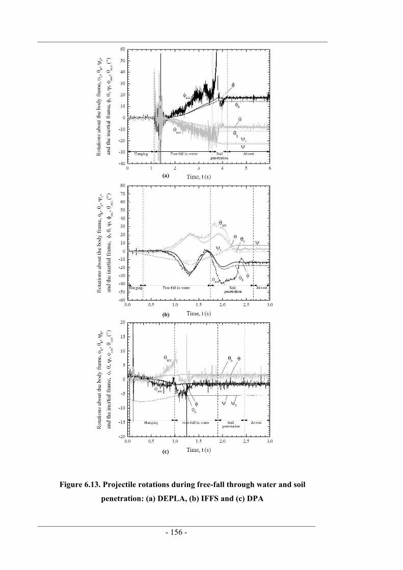
- 156 -
Figure 6.13. Projectile rotations during free-fall through water and soil
penetration: (a) DEPLA, (b) IFFS and (c) DPA
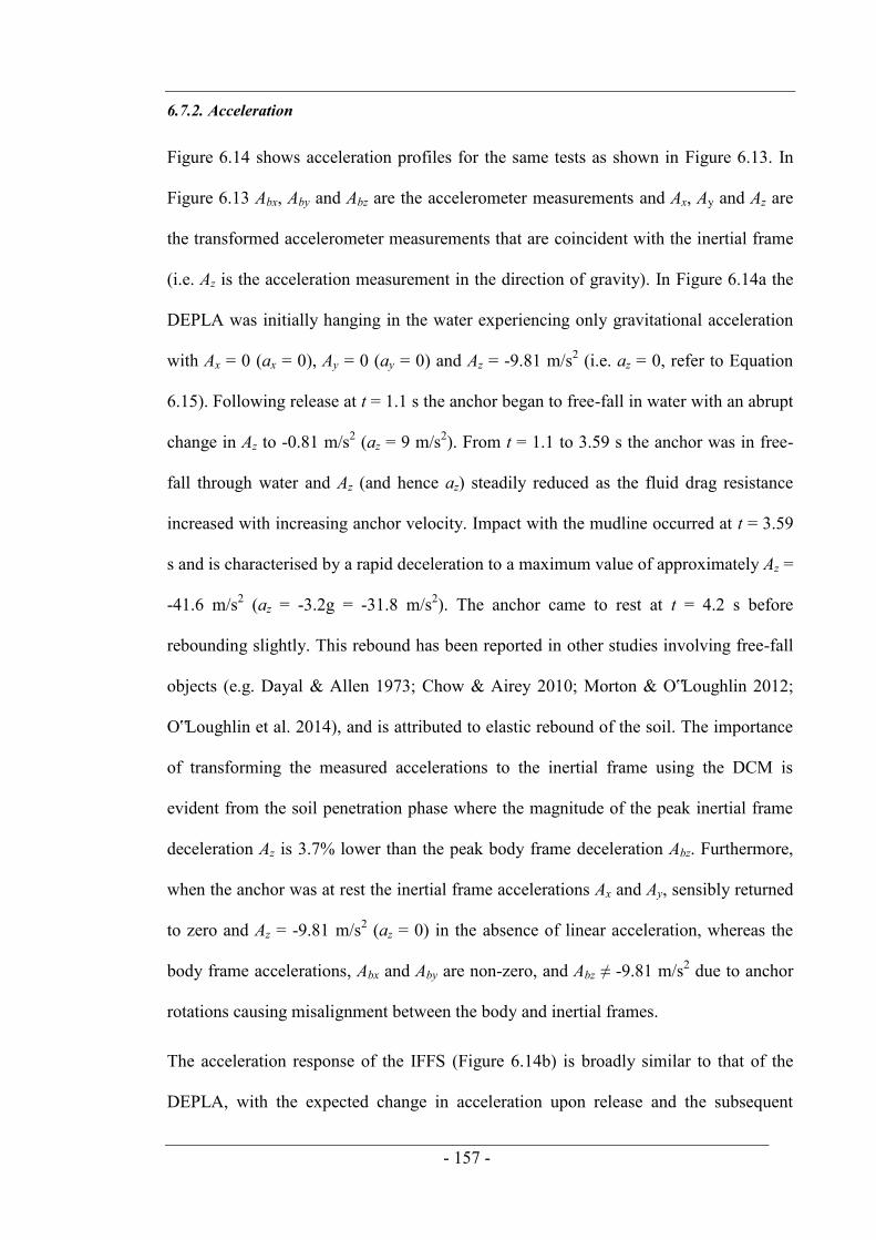
- 157 -
6.7.2. Acceleration
Figure 6.14 shows acceleration profiles for the same tests as shown in Figure 6.13. In
Figure 6.13 Abx, Aby and Abz are the accelerometer measurements and Ax, Ay and Az are
the transformed accelerometer measurements that are coincident with the inertial frame
(i.e. Az is the acceleration measurement in the direction of gravity). In Figure 6.14a the
DEPLA was initially hanging in the water experiencing only gravitational acceleration
with Ax = 0 (ax = 0), Ay = 0 (ay = 0) and Az = -9.81 m/s2 (i.e. az = 0, refer to Equation
6.15). Following release at t = 1.1 s the anchor began to free-fall in water with an abrupt
change in Az to -0.81 m/s2 (az = 9 m/s2). From t = 1.1 to 3.59 s the anchor was in free-
fall through water and Az (and hence az) steadily reduced as the fluid drag resistance
increased with increasing anchor velocity. Impact with the mudline occurred at t = 3.59
s and is characterised by a rapid deceleration to a maximum value of approximately Az =
-41.6 m/s2 (az = -3.2g = -31.8 m/s2). The anchor came to rest at t = 4.2 s before
rebounding slightly. This rebound has been reported in other studies involving free-fall
objects (e.g. Dayal & Allen 1973; Chow & Airey 2010; Morton & O‟Loughlin 2012;
O‟Loughlin et al. 2014), and is attributed to elastic rebound of the soil. The importance
of transforming the measured accelerations to the inertial frame using the DCM is
evident from the soil penetration phase where the magnitude of the peak inertial frame
deceleration Az is 3.7% lower than the peak body frame deceleration Abz. Furthermore,
when the anchor was at rest the inertial frame accelerations Ax and Ay, sensibly returned
to zero and Az = -9.81 m/s2 (az = 0) in the absence of linear acceleration, whereas the
body frame accelerations, Abx and Aby are non-zero, and Abz ≠ -9.81 m/s2 due to anchor
rotations causing misalignment between the body and inertial frames.
The acceleration response of the IFFS (Figure 6.14b) is broadly similar to that of the
DEPLA, with the expected change in acceleration upon release and the subsequent
- 158 -
reduction in acceleration due to increasing fluid drag resistance. Accelerations also
reduce markedly upon impact with the soil surface, although the absolute deceleration is
lower than for the DEPLA due to the lower soil strength at this site. The sudden
reduction in the accelerations along the z-axis during penetration in soil (evident in both
the body frame and the inertial frame accelerations) is considered to be due to changes
in the soil flow regime. This influences the magnitude of the drag resistance that
dominates at these very shallow embedment depths in very soft soil and at high
penetration velocities (Morton et al. 2015).
Figure 6.14c shows the acceleration response for the DPA test. The response is
qualitatively similar to those shown in Figure 6.14a and Figure 6.14b for the DEPLA
and the IFFS respectively, although there is negligible difference between the body
frame accelerations and the transformed inertial frame accelerations as rotations where
relatively small for this test.
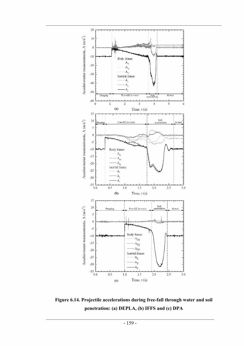
- 159 -
Figure 6.14. Projectile accelerations during free-fall through water and soil
penetration: (a) DEPLA, (b) IFFS and (c) DPA

- 160 -
6.7.3. Velocity profiles
Figure 6.15 shows velocity profiles for free-fall in water and embedment into soil for
the three tests considered previously and shown in Figures 13 and 14. The velocity vz,
and distance sz, (i.e. depth) relative to the inertial frame were established using
Equations 6.19 and 6.20. The velocity vbz, and distance zbz, were also derived from
Equations 6.19 and 6.20, albeit with abz = Abz + g, instead of az and Az. vbz and zbz
represent the values that would otherwise be used if the IMU measurements were not
corrected using the AVTM and DCM. The importance of implementing the
transformation matrices is demonstrated in Figure 6.15a where the final embedment
depth and impact velocity of the DEPLA are over estimated by 12% and 7%
respectively. This would correspond to an over prediction of the local undrained shear
strength (and hence capacity) at the mid-height of the DEPLA plate (following
installation but prior to keying) of 17% based on the final tip embedment of ze = 3.31 m
and the idealised strength profile, su (kPa) = 2 + 2.8z. Figure 6.15b indicates that the
embedment depth and impact velocity of the IFFS are over predicted by 27% and 10%
respectively. The over prediction for the IFFS is higher than for the DEPLA as the IFFS
rotations are higher (i.e. greater misalignment between the body- and inertial frames).
Figures 15a and 15b also show that the velocity vbz, established from the integration of
the body frame „linear‟ acceleration abz, does not return to zero despite motion having
ceased. This is because the body frame acceleration measurement Abz, (from which abz is
derived) is not coincident with the inertial frame and does not return to zero following
installation (i.e. Abz > -9.81 m/s2). The DPA body frame and inertial frame velocity
profiles (Figure 6.15c) are in excellent agreement as the rotations are relatively low and
the misalignment between the body frame and inertial frame is negligible. Also shown
on Figure 6.15 are direct measurements of the final embedment depths based on

- 161 -
mudline observations of markings on the retrieval line using a ROV in Firth of Clyde
and an underwater drop camera in Lough Erne. Final embedment depths derived from
the IMU data are within 3.3% of the direct measurements, with differences of 0.09 m
(DEPLA), 0.06 m (IFFS) and 0.035 m (DPA). However, the direct measurements are
simply to confirm the lack of any gross error in the analysis, and have a much lower
accuracy than is possible from the IMU data. A more rigorous verification of the IMU
derived measurements was undertaken for a number of tests as described in the
following section.
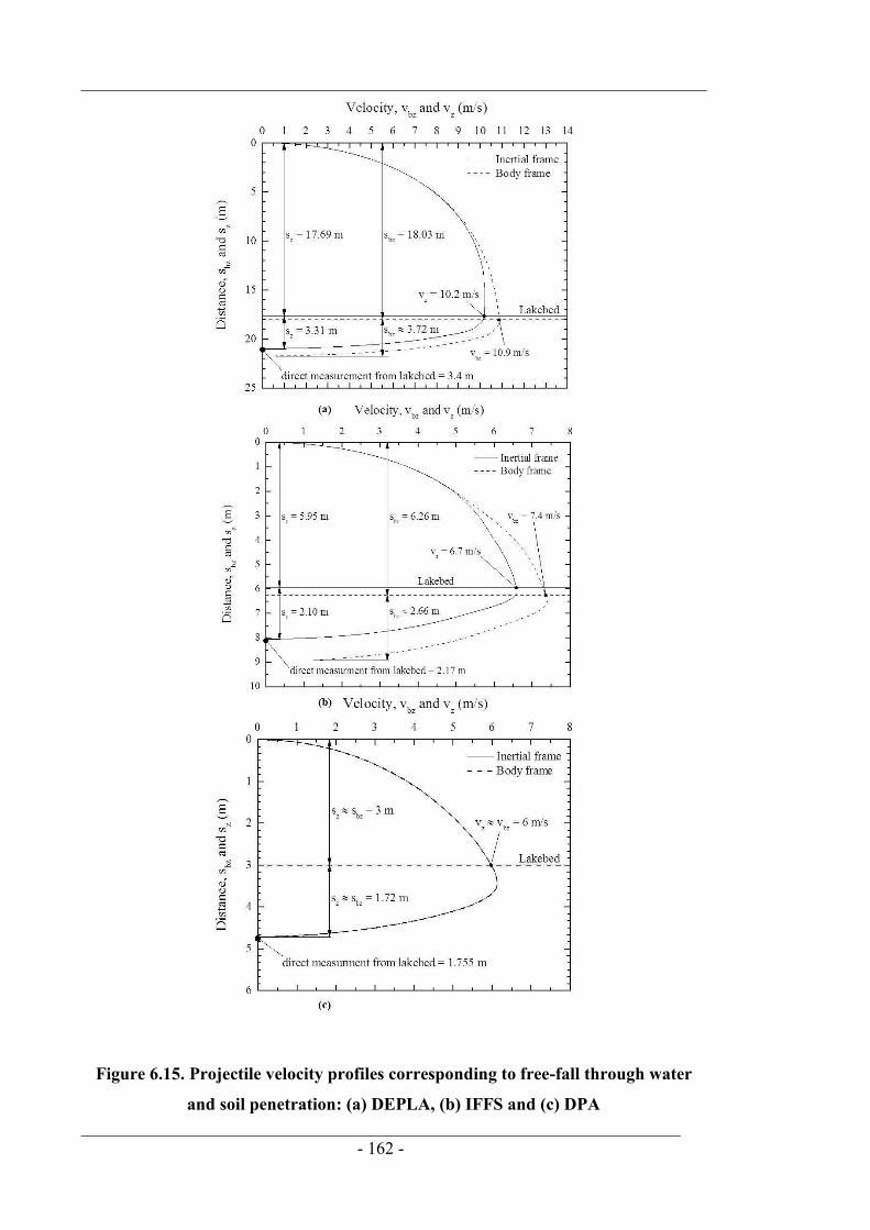
- 162 -
Figure 6.15. Projectile velocity profiles corresponding to free-fall through water
and soil penetration: (a) DEPLA, (b) IFFS and (c) DPA
- 163 -
6.7.4. Verification of the IMU derived measurements
Independent verification of the IMU-derived measurements of the projectile
displacement (Equation 6.22) was obtained by comparison with those obtained from a
draw wire sensor (also known as a string potentiometer) with a 10 m measurement
range. The draw wire sensor was connected between a fixed point on the deployment
platform and the free falling projectile (i.e. in parallel with the deployment and retrieval
line), and the data acquired using an independent 24-bit data acquisition system. Five
tests were undertaken using the IFFS projectile released from 0 to 4.8 m above the
lakebed.
Comparisons of displacements derived from the IMU measurements and the draw wire
sensor data are provided in Figure 6.16. The IMU-derived displacements are shown
both using the body reference frame and the inertial reference frame. This shows that
the inertial frame-derived displacements correctly remain constant when the projectile
comes to rest in the soil. In contrast, the body frame-derived displacements continue to
increase as the resultant linear acceleration, a, has not returned to zero due to the
rotation of the body (see also Figure 6.15). Importantly, excellent agreement is apparent
between the inertial frame displacements and those measured by the draw wire sensor
(within 1% of the measurement range), providing verification of the analysis approach
outlined here.

- 164 -
Figure 6.16. Comparision of IMU derived displacement measurements with those
obtained using a draw wire sensor
6.7.5. Example application of projectile IMU data
For the projectiles considered in the previous section, understanding the soil-structure
interaction at such high strain rates is crucial for predictive tools that calculate the final
embedment depth of the anchors (DEPLA and DPA, e.g. O‟Loughlin et al. 2013b) or
estimate the undrained shear strength based on the interpreted inertial frame
accelerations (IFFS, O‟Loughlin et al. 2014; Morton et al. 2015). This is because those
strain rates are up to seven orders of magnitude higher than used for strength
determination in a standard laboratory element test. It follows that motion data such as
those presented in Figure 6.13 and Figure 6.14 play an important role in the validation
and calibration of such predictive models. An example comparison is provided in Figure
6.17 for the DEPLA, where the predictions are based on an analytical model described

- 165 -
in brief here, but in more detail by O‟Loughlin et al. (2013b). The model formulates
conventional end bearing and frictional resistance acting on the anchor during
penetration in a manner similar to suction caisson or pile installation, but scales these
resistances to account for the well-known dependence of undrained shear strength on
strain rate (Casagrande & Wilson 1951, Graham et al. 1983, Sheahan et al. 1996), whilst
also accounting for drag resistance and the buoyant weight of the displaced soil.
Consideration of these resistance components leads to the following governing
equation:
dbearbearffrictfrictfbs FFRFRFWdt
sdm ,,2
2
6.26
where m is the anchor mass, s is the distance travelled by the projectile, t is time, Ws is
the submerged weight of the anchor in water, Ffrict is frictional resistance, Fbear is
bearing resistance, Fb is the buoyant weight of the displaced soil, Rf,frict and Rf,bear the
strain rate function associated with the bearing and frictional resistance and Fd is drag
resistance, formulated as:
2
21 vACF psdd 6.27
where s is the submerged density of the soil, Cd is the drag coefficient, Ap is anchor
projected (frontal) area and v is the instantaneous resultant anchor velocity. The
inclusion of fluid drag, Fd, is essential in situations where (non-Newtonian) very soft
fluidised soil is encountered at the surface of the seabed, and has been shown to be
important for assessing loading from a submarine slide runout on a pipeline (Boukpeti

- 166 -
et al. 2012, Einav & Randolph, 2006, White 2012, Sahdi et al. 2014). O‟Loughlin et al.
(2013) and Blake & O‟Loughlin (2015) further showed that drag is the dominant
resistance acting on a dynamically installed anchor in normally consolidated clay during
initial embedment and typically to about 30% of the penetration.
Frictional and bearing resistances are formulated as:
sufrict AsF 6.28
pubear ANsF 6.29
where α is an interface friction ratio (of limiting shear stress to undrained shear
strength), As is anchor shaft area, N is the bearing capacity factor for the projectile tip or
fluke, and su is the undrained shear strength averaged over the contact area, Ap or As.
The reference undrained shear strength adopted in Equation 6.28 is the idealised profile
shown in Figure 6.9a, which is enhanced using a power law strain rate function
(Biscontin & Pestena 2001; Peuchan & Mayne 2007; Randolph et al. 2007; O‟Loughlin
et al. 2013b) expressed as:
refreff dv
dvnR
6.30
where β is the strain rate parameter, v/d is an approximation of the operational shear
strain rate, and the subscript „ref‟ denotes the reference shear strain rate associated with
the measurement of the undrained shear strength. The factor n in Equation 6.30
accounts for the greater rate effects reported for shaft resistance compared to tip
resistance (Dayal et al., 1975; Chow et al., 2014; Steiner et al. 2014) and is taken as n =
- 167 -
1 for tip resistance (Zhu & Randolph, 2011) and as a function of (adopted from
Equation 8b in Einav & Randolph, 2006) for estimating rate effects in shaft resistance
according to:
22 l
l nβnn 6.31
where nl is 1 for axial loading.
The predictions on Figure 6.17 were obtained using bearing capacity factors of N = 7.5
for the leading and trailing edges of the flukes (analogous to a deeply embedded strip
footing) and N = 12 for the follower tip, but not for the padeye as the hole formed by the
passage of the anchor was assumed to remain open. This is appropriate since ROV
video capture of the drop sites (see Figure 6.12) showed an open crater and the
dimensionless strength ratio at the trailing end of the embedded DEPLA follower, su/γ'd
= 6.9 (where d is the diameter of the DEPLA sleeve and γ' is the effective unit weight of
the soil), which is sufficient to maintain an open cavity above the follower (Morton et
al. 2014). Values for the drag coefficient, Cd, were determined from the free-fall in
water phase of the tests, which gave an average Cd = 0.7 (Blake & O‟Loughlin, 2015).
The strain rate parameter was taken as β = 0.08, which is typical of that measured in
variable rate penetrometer testing (Low et al. 2008, Lehane et al. 2009) and
approximates to an 18% change per log cycle change in strain rate, typical of that
measured in laboratory testing (e.g. Vaid & Campenella 1977, Graham et al. 1983,
Lefebvre & Leboeuf 1987). The interface friction ratio, α, was varied to obtain the best
match between the measured and predicted velocity profiles. The comparison between
these on Figure 6.17 indicates that the inclusion of a fluid-mechanics drag resistance
term is appropriate for projectiles penetrating soft clay at high velocities. There is
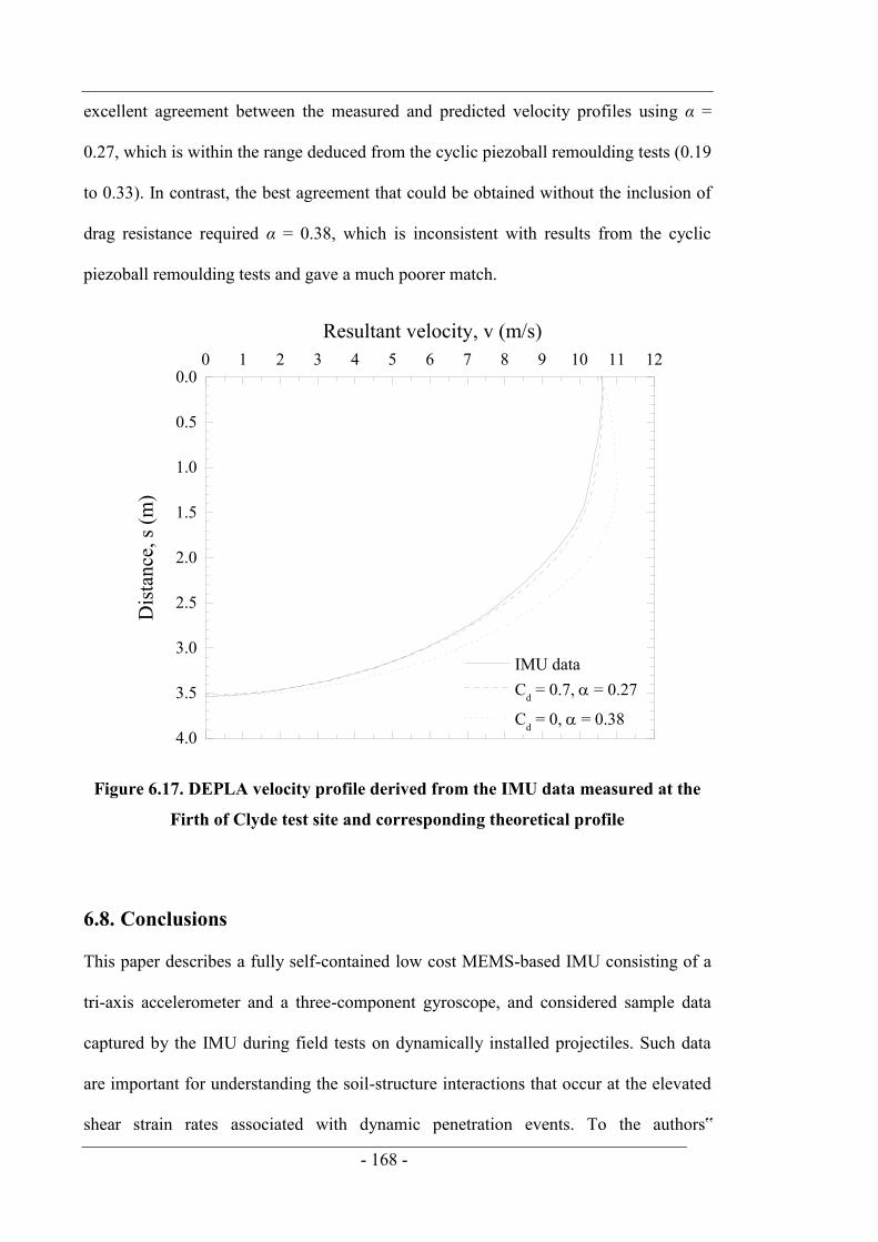
- 168 -
excellent agreement between the measured and predicted velocity profiles using α =
0.27, which is within the range deduced from the cyclic piezoball remoulding tests (0.19
to 0.33). In contrast, the best agreement that could be obtained without the inclusion of
drag resistance required α = 0.38, which is inconsistent with results from the cyclic
piezoball remoulding tests and gave a much poorer match.
Figure 6.17. DEPLA velocity profile derived from the IMU data measured at the
Firth of Clyde test site and corresponding theoretical profile
6.8. Conclusions
This paper describes a fully self-contained low cost MEMS-based IMU consisting of a
tri-axis accelerometer and a three-component gyroscope, and considered sample data
captured by the IMU during field tests on dynamically installed projectiles. Such data
are important for understanding the soil-structure interactions that occur at the elevated
shear strain rates associated with dynamic penetration events. To the authors‟
0 1 2 3 4 5 6 7 8 9 10 11 12
4.0
3.5
3.0
2.5
2.0
1.5
1.0
0.5
0.0
IMU data Cd = 0.7, = 0.27
Cd = 0, = 0.38
Resultant velocity, v (m/s)
Dis
tanc
e, s
(m)

- 169 -
knowledge these data are the first reported use of a 6DoF IMU for a geotechnical
application.
A comprehensive framework for interpreting the IMU measurements so that they are
coincident with a fixed inertial frame of reference was described and implemented to
establish projectile rotations, accelerations and velocities during free-fall in water and
embedment in soil. It is often the final embedment depth of a dynamically embedded
projectile that is of interest. The paper showed that for projectiles that tilt during free-
fall, embedments calculated from the body frame acceleration measurements, rather
than from accelerations transformed to an inertial frame of reference, led to derived
embedment depths that were in error by up to 27%. In contrast, embedment depths
derived from IMU data interpreted from within an inertial frame of reference were
shown to be in excellent agreement with independent direct measurements.
The merit of collecting motion data during dynamic penetration events was
demonstrated by using the IMU data to validate an embedment prediction model based
on strain rate enhanced shear resistance and fluid mechanics drag resistance for
dynamically installed anchors. In this demonstration the inclusion of drag resistance
during embedment in soil was shown to be appropriate, as the measured and predicted
velocity profiles were in excellent agreement. In contrast, when drag resistance was
omitted an interface friction ratio inconsistent with the measured soil sensitivity was
required to match the final embedment depth, and as a consequence the overall
agreement between the measured and predicted profiles was much poorer.
In conclusion, the use of a reliable IMU with an appropriate interpretation framework is
required to successfully apply these projectile-based geotechnical devices.

- 170 -
CHAPTER 7. ESTIMATION OF SOIL STRENGTH BY
INSTRUMENTED FREE-FALL SPHERE TESTS
7.1. Abstract
Dynamic penetration of rigid bodies into soil is a complex problem as it involves
inertial effects and extreme strain rates that enhance the soil strength. The dynamic
response of a sphere in soft clay is considered in this paper through field tests in which a
0.25 m diameter steel sphere was allowed to free-fall in water and dynamically
penetrate the underlying soft soil. The test data, which were collected in a lake and a
nearshore environment, relate to sphere velocities of up to 8 m/s, reaching sphere invert
This chapter extends Chapter 3 by further reporting field test data measured in IFFS
tests at two soft soil sites. The measurement technique introduced in Chapter 6 for
interpreting the IMU data is used to interpret the net penetration resistance acting on
the IFFS that extends the simplified model described in Chapter 3 and also
incorporates the shallow penetration framework described in Chapter 4. The
framework allows the undrained shear strength, su, to be devised from the IFFS net
penetration resistance and the chapter concludes by comparing these measurements
with those obtained in equivalent pushed-in ball penetration tests.
Morton, J. P., O‟Loughlin, C. D. & White. D. J., 2015. Field testing an in situ
freefalling spherical penetrometer in soft soil. Submitted to Géotechnique.
- 171 -
embedments close to 10 diameters. An interial measurement unit located within the
sphere measured the motion response of the sphere during free-fall and penetration in
soil. The resulting acceleration data were used within a simple framework that accounts
for both geotechnical shearing resistance and fluid mechanics drag resistance, but cast
in terms of a single capacity factor that can be expressed in terms of the non-Newtonian
Reynolds number. The merit of the framework is demonstrated by using it as a forward
model in a series of inverse analyses that calculate the undrained shear strength profile
from acceleration data measured in free-fall sphere tests. The good match between these
profiles and those obtained from push-in piezoball penetrometer tests point to the
potential for an Instrumented Free-Fall Sphere (IFFS) to be used a tool for charcterising
the near surface strength of soft seabeds.
7.2. Introduction
Geotechnical aspects of offshore and near-shore infrastructure projects often involve the
assesment of complex soil-structure interactions involving strain rates than are often
several orders of magnitude higher than those associated with laboratory element tests.
The most extreme examples relate to dynamic impact events such as submarine
landslide runout on pipelines and installation of free-fall projectiles such as soil
samplers, penetrometers for soil strength estimation and dynamically installed anchors.
Such problems require an assessment of the net dynamic penetration resistance, which
can generally be resolved into two separate components. The first is the strain-rate
dependant geotechnical component (comprising the bearing resistance and for slender
projectiles, frictional resistance) which represents the strength-dominated domain, and
the second is the fluid dynamics component, which is the drag resistance that represents
the inertia-dominated domain. Morton & O‟Loughlin (2012) adopt this „summation‟
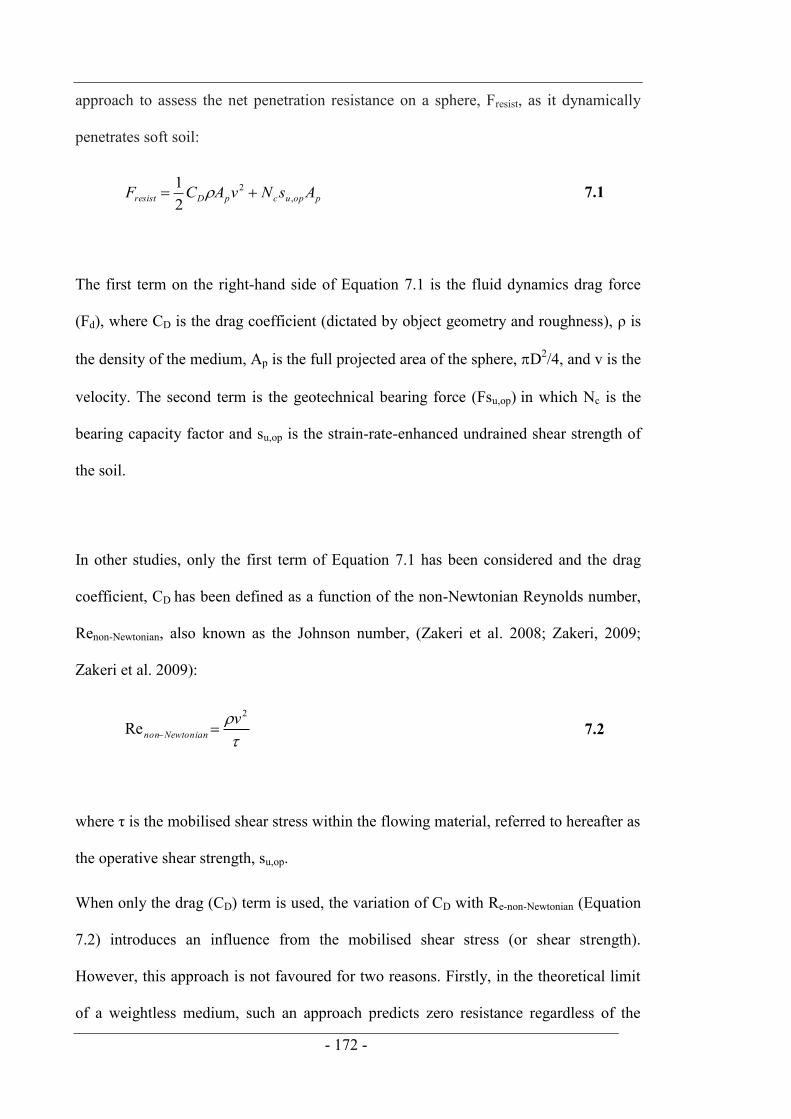
- 172 -
approach to assess the net penetration resistance on a sphere, Fresist, as it dynamically
penetrates soft soil:
popucpDresist AsNvACF ,2
21
7.1
The first term on the right-hand side of Equation 7.1 is the fluid dynamics drag force
(Fd), where CD is the drag coefficient (dictated by object geometry and roughness), ρ is
the density of the medium, Ap is the full projected area of the sphere, D2/4, and v is the
velocity. The second term is the geotechnical bearing force (Fsu,op) in which Nc is the
bearing capacity factor and su,op is the strain-rate-enhanced undrained shear strength of
the soil.
In other studies, only the first term of Equation 7.1 has been considered and the drag
coefficient, CD has been defined as a function of the non-Newtonian Reynolds number,
Renon-Newtonian, also known as the Johnson number, (Zakeri et al. 2008; Zakeri, 2009;
Zakeri et al. 2009):
2
Re vNewtoniannon 7.2
where τ is the mobilised shear stress within the flowing material, referred to hereafter as
the operative shear strength, su,op.
When only the drag (CD) term is used, the variation of CD with Re-non-Newtonian (Equation
7.2) introduces an influence from the mobilised shear stress (or shear strength).
However, this approach is not favoured for two reasons. Firstly, in the theoretical limit
of a weightless medium, such an approach predicts zero resistance regardless of the
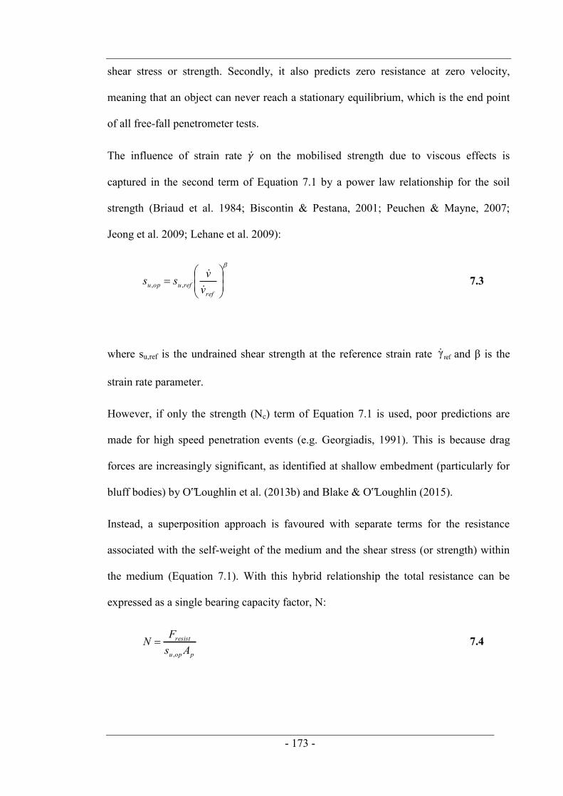
- 173 -
shear stress or strength. Secondly, it also predicts zero resistance at zero velocity,
meaning that an object can never reach a stationary equilibrium, which is the end point
of all free-fall penetrometer tests.
The influence of strain rate on the mobilised strength due to viscous effects is
captured in the second term of Equation 7.1 by a power law relationship for the soil
strength (Briaud et al. 1984; Biscontin & Pestana, 2001; Peuchen & Mayne, 2007;
Jeong et al. 2009; Lehane et al. 2009):
refrefuopu v
vss
,, 7.3
where su,ref is the undrained shear strength at the reference strain rate refγ and β is the
strain rate parameter.
However, if only the strength (Nc) term of Equation 7.1 is used, poor predictions are
made for high speed penetration events (e.g. Georgiadis, 1991). This is because drag
forces are increasingly significant, as identified at shallow embedment (particularly for
bluff bodies) by O‟Loughlin et al. (2013b) and Blake & O‟Loughlin (2015).
Instead, a superposition approach is favoured with separate terms for the resistance
associated with the self-weight of the medium and the shear stress (or strength) within
the medium (Equation 7.1). With this hybrid relationship the total resistance can be
expressed as a single bearing capacity factor, N:
popu
resist
AsFN
,
7.4
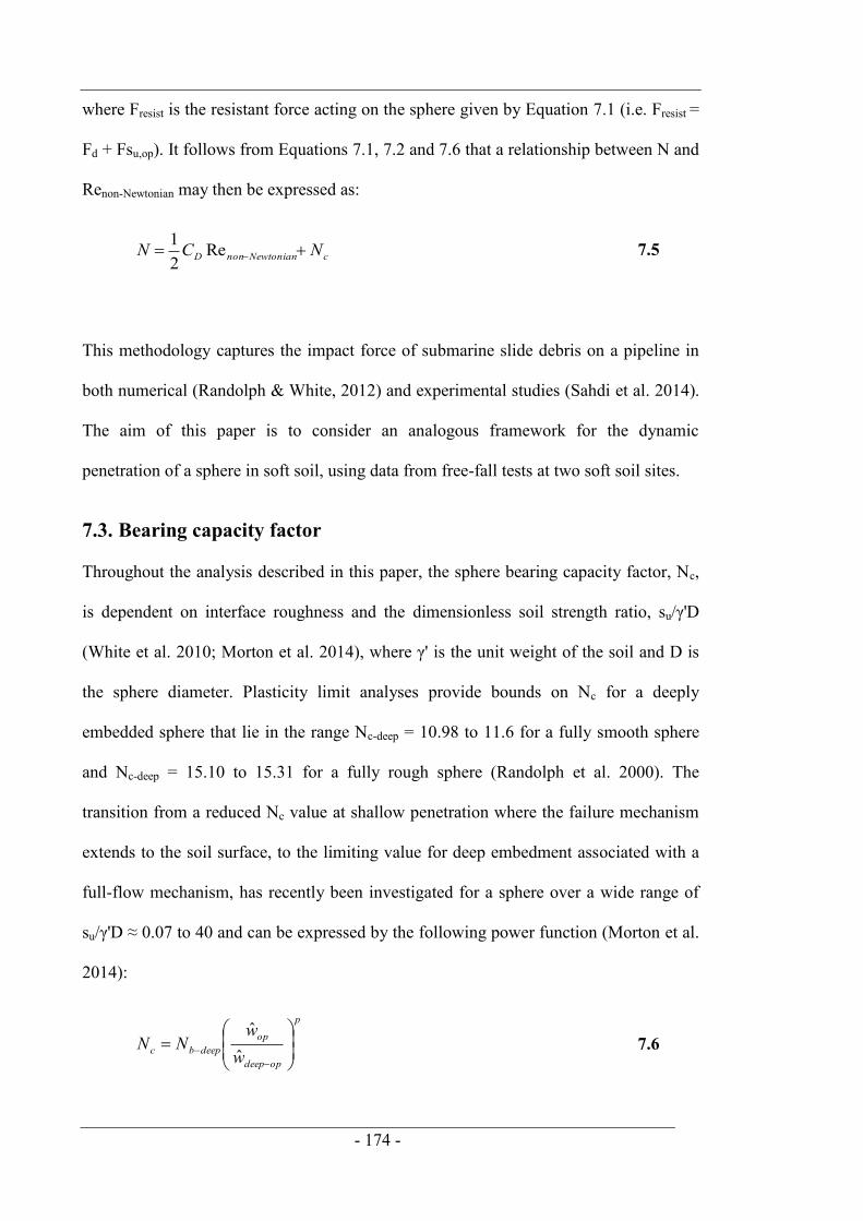
- 174 -
where Fresist is the resistant force acting on the sphere given by Equation 7.1 (i.e. Fresist =
Fd + Fsu,op). It follows from Equations 7.1, 7.2 and 7.6 that a relationship between N and
Renon-Newtonian may then be expressed as:
cNewtoniannonD NCN Re21 7.5
This methodology captures the impact force of submarine slide debris on a pipeline in
both numerical (Randolph & White, 2012) and experimental studies (Sahdi et al. 2014).
The aim of this paper is to consider an analogous framework for the dynamic
penetration of a sphere in soft soil, using data from free-fall tests at two soft soil sites.
7.3. Bearing capacity factor
Throughout the analysis described in this paper, the sphere bearing capacity factor, Nc,
is dependent on interface roughness and the dimensionless soil strength ratio, su/γ'D
(White et al. 2010; Morton et al. 2014), where γ' is the unit weight of the soil and D is
the sphere diameter. Plasticity limit analyses provide bounds on Nc for a deeply
embedded sphere that lie in the range Nc-deep = 10.98 to 11.6 for a fully smooth sphere
and Nc-deep = 15.10 to 15.31 for a fully rough sphere (Randolph et al. 2000). The
transition from a reduced Nc value at shallow penetration where the failure mechanism
extends to the soil surface, to the limiting value for deep embedment associated with a
full-flow mechanism, has recently been investigated for a sphere over a wide range of
su/γ'D ≈ 0.07 to 40 and can be expressed by the following power function (Morton et al.
2014):
p
opdeep
opdeepbc w
wNN
ˆˆ
7.6
- 175 -
where the transitional depth at which Nc = Nc-deep is given by
f
u
cu
opdeep
eD
s
adD
sbaw
/1
ˆ
7.7
and the fitting constants a = 16.3, b = 0.12, c = 1.3, d =0.52, e = 4.9, f = 1.5 and p =
0.49.
7.4. Site description and soil properties
The Instrumented Free-Fall Sphere (IFFS) tests were conducted at two sites; the first
was Lough Erne which is a freshwater lake in County Fermanagh, Northern Ireland and
the second was Firth of Clyde, which is located off the West coast of Scotland between
the mainland and the Isle of Cumbrae. Water depths at the testing locations were 1 to 12
m at Erne and approximately 50 m at Clyde. Classification tests were conducted on bulk
and tube samples retrieved from Erne and on piston samples retrieved from Clyde. The
lakebed at Erne is very soft clay with moisture contents in the range 270 to 520%,
typically about 1.5 times the liquid limit, and a fines fraction of 95%. The measured
bulk unit weight of the Lough Erne clay is only marginally higher than water at γ = 10.8
kN/m3. This is due to the very high proportion of diatoms that are evident from
scanning electron microscopic images of the soil (Colreavy et al. 2012). These diatoms
have an enormous capacity to hold water in the intraskeletal pore space (Tanaka &
Locat, 1999). However the water that rests within this pore space is not considered to
play a role in soil behaviour, and as such the measured unit weight and other index
properties that are expressed in terms of the measured moisture content are not
considered to be useful indicators of soil behaviour. The seabed at Clyde is also very
soft, with moisture contents in the range 50 to 100% (close to the liquid limit) and a

- 176 -
fines fraction of 80%. Consistency limits plot above or on the A-line on the Casagrande
plasticity chart, indicating a clay of intermediate to high plasticity. The bulk unit weight
increases from about γ = 14 kN/m3 at the mudline to about γ = 18 kN/m3 at about 3.5 m
(limit of the sampling depth).
Figure 7.1a and b shows profiles of undrained shear strength, su, with depth derived
from piezoball penetrometer tests and a combination of in situ vane tests (Erne),
laboratory vane tests (Clyde) and fall cone tests (Clyde) The piezoball tests used a
penetrometer with a ball diameter of 113 mm in Erne and ball diameters of 113 and 80
mm in Clyde. An exact 10:1 ratio between the ball and shaft areas was maintained for
all penetration tests by using different shafts for each piezoball. A penetration rate of 20
mm/s (as is standard for cone testing) was adopted in an attempt to obtain undrained
conditions during penetration. The best agreement between the piezoball profiles and
the other strength measurements was obtained using Nc-deep = 11.8 for Clyde and Nc-deep
= 8.5 for Erne.

- 177 -
Figure 7.1. Undrained shear strength profiles in: (a) Lough Erne and (b) Firth of
Clyde

- 178 -
7.5. Test equipment and testing procedures
7.5.1. Instrumented free-fall sphere
The custom-made Instrumented Free-Fall Sphere (IFFS, see Figure 2a and 2c) is 250
mm in diameter and consists of two mild steel hemispheres that bolt together. An O-ring
located between the two hemispheres prevents the ingress of water to protect an inertial
measurement unit (IMU, described in the following section) that can be located within
vertical cylindrical voids in each hemisphere. The sphere and IMU have a dry mass, m
= 51.25 kg and an effective mass when submerged in fresh water of 43.07 kg. A 12 mm
diameter Dyneema SK75 rope was used for deploying and recovering the IFFS.
Figure 7.2. Instrumented free-fall sphere: (a) sphere separated with IMU located
within internal void, (b) IMU and (c) assembled sphere prior to a free-fall test in
Erne
7.5.2. Inertial measurement unit
The inertial measurement unit (IMU) used in the free-fall sphere tests (shown in Figure
7.2b) is a fully self-contained motion logger designed to capture the motion history of
free-fall projectiles. The IMU includes a 16-bit three component MEMS rate gyroscope
- 179 -
(ITG 3200) and a 13-bit three-axis MEMS accelerometer (ADXL 345). The gyroscope
has a resolution of 0.07 °/s with a measurement range of +/- 2000 °/s. The
accelerometer has a resolution of 0.04 m/s2 with a measurement range of +/-16 g. Data
are logged by an mbed micro controller with an ARM processor to a 2 GB SD card at
400 Hz. Internal batteries are capable of powering the logger for up to 4 hours. In the
free-fall sphere tests the IMU was contained in a watertight aluminium tube 185 mm
long and 42 mm in diameter that fitted securely within the internal cylindrical void in
the sphere.
The MEMS accelerometer measures both linear and gravitational acceleration
(depending on the sphere orientation) in three orthogonal body-frame axes that are
common to both the IMU and the sphere. In order to distinguish the sphere‟s linear
acceleration component from the acceleration detected by the sensor, which may be
slightly rotating, it is important to transform the body frame acceleration measurements
to accelerations that are coincident with the Earth-fixed inertial frame using rotation
matrices, described in detail by Blake et al. (2015). Linear accelerations corresponding
to the inertial frame z-axis (i.e. in the direction of Earth‟s gravity) were numerically
integrated to establish the sphere velocity and displacement. Figure 7.3 shows a typical
acceleration measurement of the sphere, from a hanging position to free-falling in water,
through penetration in soil, before a slight rebound due to soil elasticity (Dayal & Allen,
1973; Chow & Airey, 2010) as the sphere comes to rest. The importance of
transforming the measured accelerations to the inertial frame is evident in Figure 7.3 as
the body frame velocity is non-zero and the displacement is not constant when the
sphere is at rest. For the remainder of the paper the inertial frame z-axis linear
acceleration is referred to as the vertical acceleration.

- 180 -
Figure 7.3 IMU measurements and their interpretation from a typical free-fall
sphere test in Erne
7.5.3. Field testing procedure
The field testing program involved 87 tests that were carried out from a fixed pontoon
or a hopper barge in Erne (Figure 7.2c) and from a research and survey vessel in the
Clyde. The drop height, impact velocities and final embedments are summarised in
Table 1. The IFFS was released from various heights above the mudline to permit an
assessment of the embedment response over a range of travelling velocities. The release
height in the 72 Erne tests was varied between 0 and 9.23 m, with resulting impact
velocities in the range 0 to 7.9 m/s and sphere invert embedments of up to d = 2.373 m
(~9.5 sphere diameters). In the 15 Clyde tests, the IFFS release height was varied
between 1 and 20 m, which resulted in impact velocities between 4.0 and 6.3 m/s and
- 181 -
sphere invert embedments of up to d = 0.782 m (~ 3.13 sphere diameters). Embedment
depths were established from the IMU data as described previously, with direct
measurements based on mudline observations of markings on the retriveal line using a
remotely operated vehicle in Clyde and a drop camera in Erne. These direct
measurements were made to confirm that the analyses had not produced any gross error,
as the accuracy in the mudline obervations was much lower that was possible from the
IMU data.

- 182 -
Table 7.1. Free-fall sphere test data from the Erne tests
Test no.
Release height (m)
Impact velocity (m/s)
Sphere invert embedment depth
(m) 1 0.50 2.69 1.017 2 0.50 0.01 1.115 3 0.50 2.79 1.150 4 1.00 4.01 1.439 5 1.00 3.87 1.595 6 1.00 3.89 1.500 7 1.00 3.88 1.484 8 3.00 5.79 2.378 9 4.00 6.63 2.055 10 5.00 6.80 2.152 11 2.00 5.25 1.841 12 3.00 6.15 1.974 13 1.00 3.74 1.097 14 0.50 2.46 1.128 15 1.00 2.46 1.128 16 2.00 5.22 1.855 17 3.00 6.11 1.846 18 3.00 6.44 2.117 19 0.50 2.64 1.243 20 1.00 3.80 1.295 21 1.66 5.19 1.572 22 3.00 6.20 1.995 23 0.44 2.58 1.088 24 0.54 2.81 1.116 25 0.61 2.97 1.148 26 0.50 2.72 1.148 27 0.02 0.55 1.192 28 1.04 3.94 1.308 29 1.07 3.93 1.303 30 2.13 5.38 1.718 31 1.82 5.23 1.620 32 2.22 5.70 1.456 33 2.00 4.86 1.613 34 2.62 6.15 1.732 35 2.55 6.30 1.956 36 2.84 6.35 1.804 37 2.61 6.51 1.788 38 2.47 6.14 1.803 39 3.39 6.63 1.889 40 0.50 2.67 0.918 41 0.84 3.68 1.183
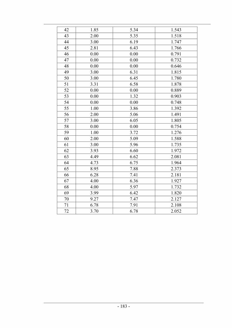
- 183 -
42 1.85 5.34 1.543 43 2.00 5.35 1.518 44 3.00 6.19 1.747 45 2.81 6.43 1.766 46 0.00 0.00 0.791 47 0.00 0.00 0.732 48 0.00 0.00 0.646 49 3.00 6.31 1.815 50 3.00 6.45 1.780 51 3.31 6.58 1.878 52 0.00 0.00 0.889 53 0.00 1.32 0.903 54 0.00 0.00 0.748 55 1.00 3.86 1.392 56 2.00 5.06 1.491 57 3.00 6.05 1.805 58 0.00 0.00 0.754 59 1.00 3.72 1.276 60 2.00 5.09 1.588 61 3.00 5.96 1.735 62 3.93 6.60 1.972 63 4.49 6.62 2.081 64 4.73 6.75 1.964 65 8.95 7.88 2.373 66 6.28 7.41 2.181 67 4.00 6.36 1.927 68 4.00 5.97 1.732 69 3.99 6.42 1.820 70 9.27 7.47 2.127 71 6.78 7.91 2.108 72 3.70 6.78 2.052
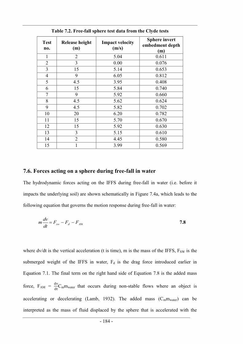
- 184 -
Table 7.2. Free-fall sphere test data from the Clyde tests
Test no.
Release height (m)
Impact velocity (m/s)
Sphere invert embedment depth
(m) 1 2 5.04 0.611 2 3 0.00 0.076 3 15 5.14 0.653 4 9 6.05 0.812 5 4.5 3.95 0.408 6 15 5.84 0.740 7 9 5.92 0.660 8 4.5 5.62 0.624 9 4.5 5.82 0.702 10 20 6.20 0.782 11 15 5.70 0.670 12 15 5.92 0.630 13 3 5.15 0.610 14 2 4.45 0.580 15 1 3.99 0.569
7.6. Forces acting on a sphere during free-fall in water
The hydrodynamic forces acting on the IFFS during free-fall in water (i.e. before it
impacts the underlying soil) are shown schematically in Figure 7.4a, which leads to the
following equation that governs the motion response during free-fall in water:
AMdsw FFFdtdvm 7.8
where dv/dt is the vertical acceleration (t is time), m is the mass of the IFFS, FSW is the
submerged weight of the IFFS in water, Fd is the drag force introduced earlier in
Equation 7.1. The final term on the right hand side of Equation 7.8 is the added mass
force, FAM =
Cmmwater that occurs during non-stable flows where an object is
accelerating or decelerating (Lamb, 1932). The added mass (Cmmwater) can be
interpreted as the mass of fluid displaced by the sphere that is accelerated with the
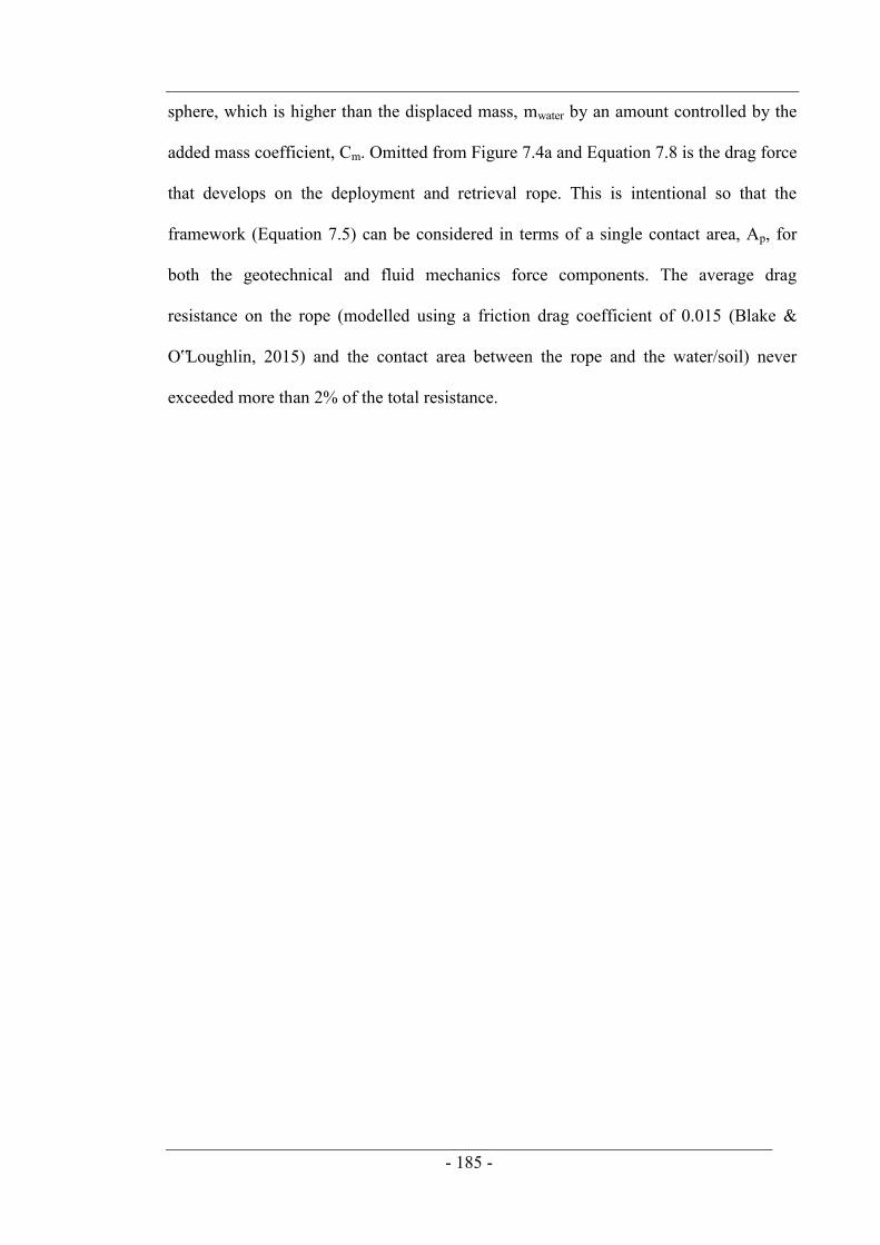
- 185 -
sphere, which is higher than the displaced mass, mwater by an amount controlled by the
added mass coefficient, Cm. Omitted from Figure 7.4a and Equation 7.8 is the drag force
that develops on the deployment and retrieval rope. This is intentional so that the
framework (Equation 7.5) can be considered in terms of a single contact area, Ap, for
both the geotechnical and fluid mechanics force components. The average drag
resistance on the rope (modelled using a friction drag coefficient of 0.015 (Blake &
O‟Loughlin, 2015) and the contact area between the rope and the water/soil) never
exceeded more than 2% of the total resistance.
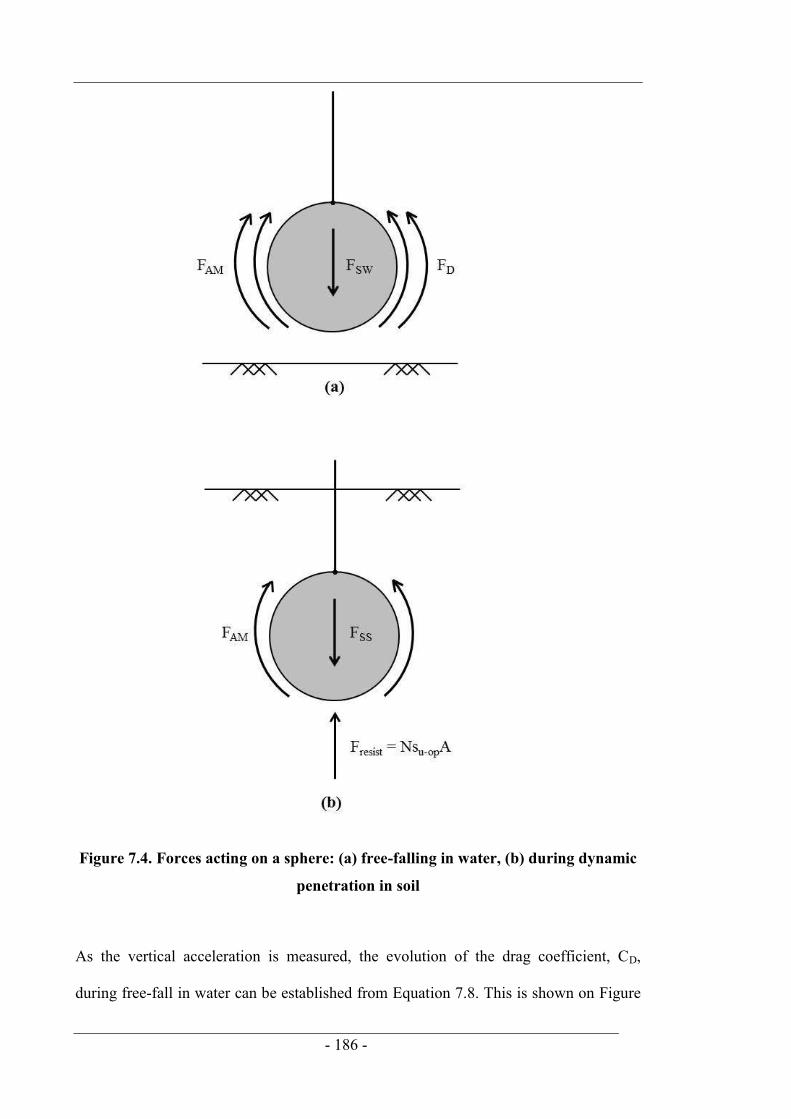
- 186 -
Figure 7.4. Forces acting on a sphere: (a) free-falling in water, (b) during dynamic
penetration in soil
As the vertical acceleration is measured, the evolution of the drag coefficient, CD,
during free-fall in water can be established from Equation 7.8. This is shown on Figure

- 187 -
7.5 for three Erne tests over a calculated range of Reynolds numbers, Re = 104 to 106
together with the empirical correlation between CD and Re proposed by Morrison
(2013), that is based on the benchmark experimental summarised by Schlichting (1955).
At lower values of Re, between Re = 104 and 105 the back-figured experimental CD is
significantly higher than empirical values of CD, and reduces rapidly with increasing Re.
However, this range of Re corresponds with the start of free-fall, with sphere velocities
less than 0.5 m/s and free-fall displacements less than 0.02 m (0.08 diameters). A
similar rapid variation in CD has been associated with the hydrodynamic response of
dynamically installed „torpedo anchors‟, immediately after the onset of free-fall
(Fernandes et al. 2006). However, at Re > 106, when the sphere velocity is > 0.5 m/s
and the free-fall displacement is typically about 0.02 m, the experimental CD values
agree well with the Morrison (2013) relationship using Cm = 0.5, which is exactly
coincident with the theoretical value for a sphere (e.g. Sumer & Fredsoe, 1997,
Pantaleone & Messer, 2011).
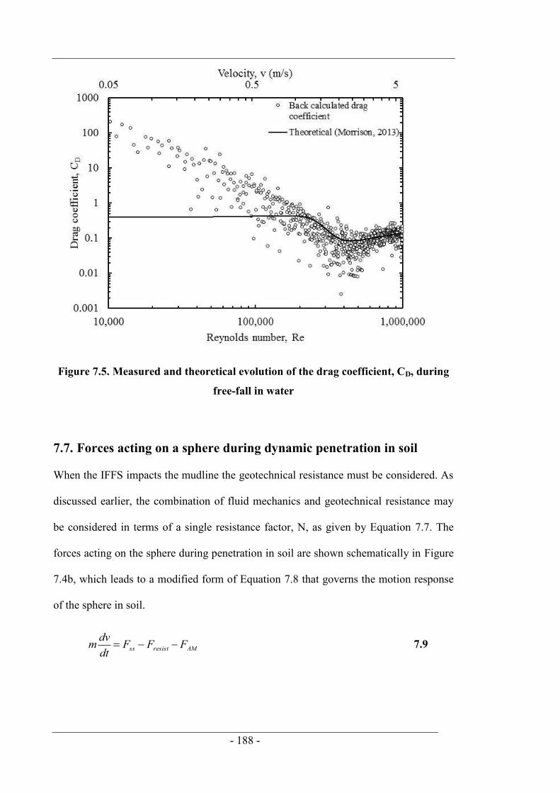
- 188 -
Figure 7.5. Measured and theoretical evolution of the drag coefficient, CD, during
free-fall in water
7.7. Forces acting on a sphere during dynamic penetration in soil
When the IFFS impacts the mudline the geotechnical resistance must be considered. As
discussed earlier, the combination of fluid mechanics and geotechnical resistance may
be considered in terms of a single resistance factor, N, as given by Equation 7.7. The
forces acting on the sphere during penetration in soil are shown schematically in Figure
7.4b, which leads to a modified form of Equation 7.8 that governs the motion response
of the sphere in soil.
AMresistss FFFdtdvm 7.9
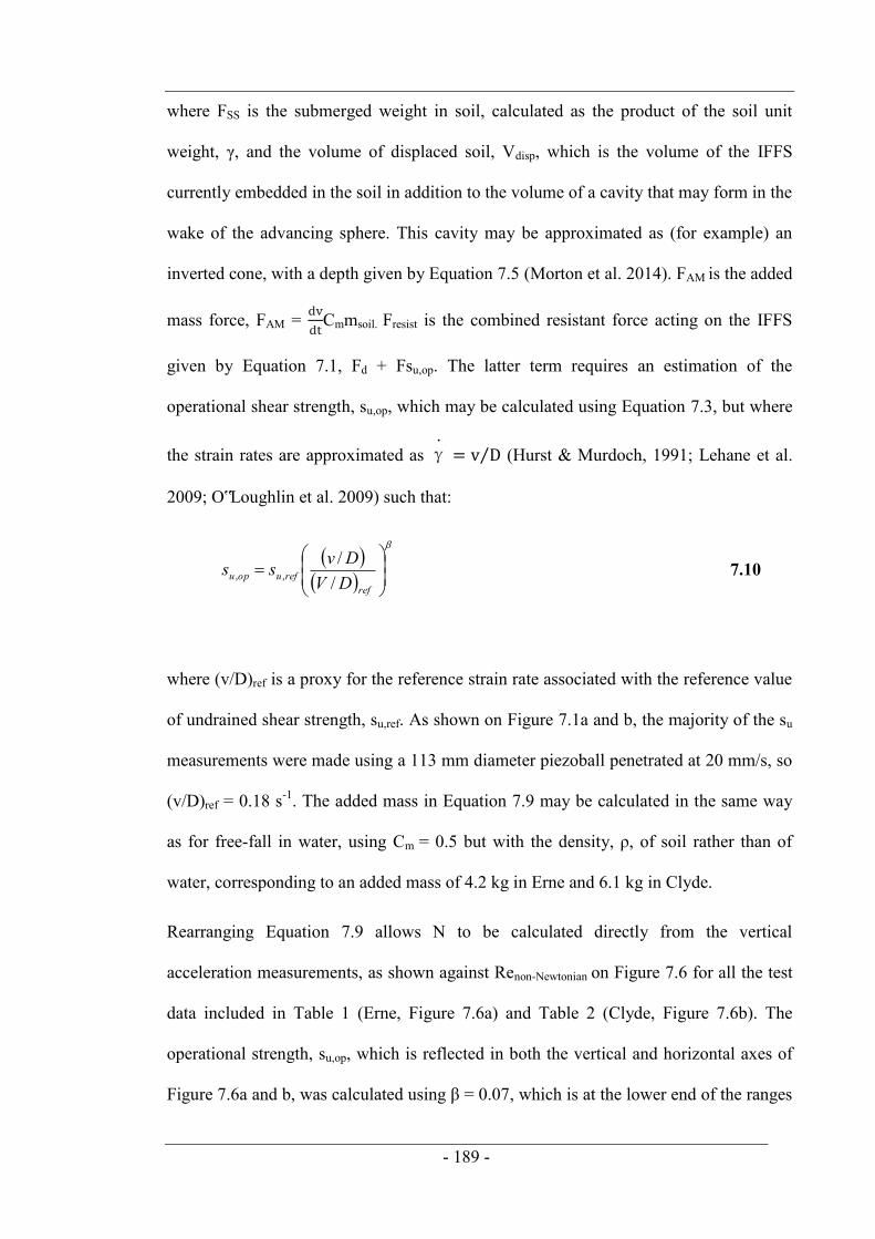
- 189 -
where FSS is the submerged weight in soil, calculated as the product of the soil unit
weight, γ, and the volume of displaced soil, Vdisp, which is the volume of the IFFS
currently embedded in the soil in addition to the volume of a cavity that may form in the
wake of the advancing sphere. This cavity may be approximated as (for example) an
inverted cone, with a depth given by Equation 7.5 (Morton et al. 2014). FAM is the added
mass force, FAM =
Cmmsoil. Fresist is the combined resistant force acting on the IFFS
given by Equation 7.1, Fd + Fsu,op. The latter term requires an estimation of the
operational shear strength, su,op, which may be calculated using Equation 7.3, but where
the strain rates are approximated as γ ⁄ (Hurst & Murdoch, 1991; Lehane et al.
2009; O‟Loughlin et al. 2009) such that:
refrefuopu DV
Dvss//
,, 7.10
where (v/D)ref is a proxy for the reference strain rate associated with the reference value
of undrained shear strength, su,ref. As shown on Figure 7.1a and b, the majority of the su
measurements were made using a 113 mm diameter piezoball penetrated at 20 mm/s, so
(v/D)ref = 0.18 s-1. The added mass in Equation 7.9 may be calculated in the same way
as for free-fall in water, using Cm = 0.5 but with the density, ρ, of soil rather than of
water, corresponding to an added mass of 4.2 kg in Erne and 6.1 kg in Clyde.
Rearranging Equation 7.9 allows N to be calculated directly from the vertical
acceleration measurements, as shown against Renon-Newtonian on Figure 7.6 for all the test
data included in Table 1 (Erne, Figure 7.6a) and Table 2 (Clyde, Figure 7.6b). The
operational strength, su,op, which is reflected in both the vertical and horizontal axes of
Figure 7.6a and b, was calculated using β = 0.07, which is at the lower end of the ranges

- 190 -
β = 0.05 to 0.17 quoted by Jeong et al. (2009) and β = 0.05 to 0.15 quoted by
O‟Loughlin et al. (2013b). β = 0.07 is consistent with a 17% increase in undrained shear
strength for every log cycle increase in shear strain rate, and is within the 10 to 20%
range commonly reported (e.g. Vaid & Campenella, 1977; Graham et al. 1983; Lefebvre
& Leboeuf, 1987).
The breadth of the range in β quoted in the literature may be (at least in part) attributed
to the order of magnitude difference between the operational strain rate and the
reference strain rate used in Equation 7.3. The maximum v/D values associated with the
IFFS tests considered here is v/D = 31 s-1, which is two orders of magnitude higher than
(v/D)ref = 0.18 s-1. This is similar to the range in v/D associated with variable rate
penetrometer and laboratory vane tests, which tend to give β values close to the lower
end of the range quoted above, e.g. β = 0.06 to 0.08 (Lehane et al. 2009) or β = 0.055
(Biscontin & Pestana, 2001).
The upper bound on Renon-Newtonian in Figure 7.6a approaches 104 in Erne and over 102 in
the Clyde. These upper bounds correspond with tests where the impact velocity was
close to the terminal velocity of the sphere and are lower for Clyde due to the higher
soil strength at the mudline when the sphere velocity is high. The lower bound Renon-
Newtonian = 10-4 and 10-1 for Erne and Clyde respectively were selected to omit the final
10 mm of embedment, where the sphere velocity was typically 0.2 m/s and the back
figured values of N begin to reduce suddenly, indicating that other forces (perhaps from
impact of the following rope or shackle) are involved.
Figure 7.6a and b highlights that at Renon-Newtonian < ~3, soil strength rather than drag is
the dominant form of resistance, whereas for Renon-Newtonian > ~3, N increases linearly
with Renon-Newtonian highlighting the dominance of drag resistance. The annotation
indicating the normalised depth (d/D) and approximate sphere velocity in Figure 7.6

- 191 -
shows that this occurs at shallow depths where the magnitude of su,op (linked to the
geotechnical component) is very low and the velocity is very high. Although the sphere
velocity is linked to both the geotechnical and fluid mechanics terms, the drag has a
much higher velocity dependency than the geotechnical term, and therefore is the
dominant form of resistance at Renon-Newtonian > ~3.
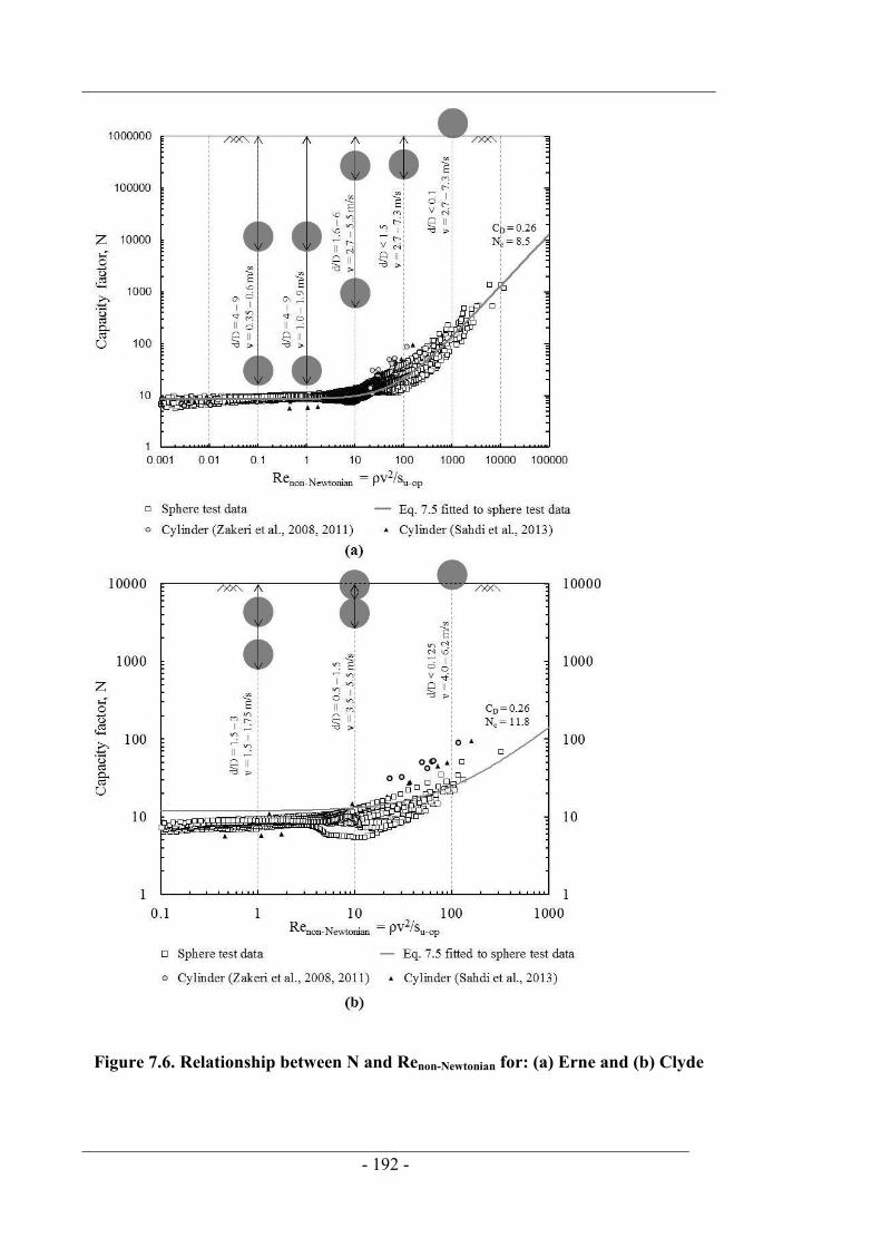
- 192 -
Figure 7.6. Relationship between N and Renon-Newtonian for: (a) Erne and (b) Clyde
- 193 -
Also shown on Figure 7.6 is the theoretical response described by Equation 7.5, which
provides a good fit to both datasets using CD = 0.26, and equivalent data for a cylinder
from experiments in a flume (Zakeri et al. 2008; Zakeri et al. 2011) and in a centrifuge
(Sahdi et al. 2014). These data exhibit the same trends as for the sphere, albeit that the
cylinder data plot above the sphere data at Renon-Newtonian > ~3, as at high Reynolds
numbers CD for a cylinder is higher than that for a sphere (Schlichting, 1955).
At Renon-Newtonian < ~3, N for the sphere occupies a wider range than for the cylinder as
the sphere. This is because the sphere embedment depth is changing, reflecting the
variation in Nc during shallow penetration (all cylinder tests were at a single
embedment). In Erne, the sphere penetrated to (on average) between 1 and 2 m,
equivalent to 4 to 8 diameters, which is sufficient in this soft soil to establish a full-flow
deep failure mechanism. The approximate range of Erne N values at Renon-Newtonian < ~3
is typically Nc-deep = 6 to 9.5, with an arithmetic mean of Nc-deep = 7.5, which is to be
expected given that the strength data input to the analyses were determined using Nc-deep
= 8.5 (as described earlier). Over the same range of at Renon-Newtonian, Clyde N values do
not reach Nc-deep = 11.8 used to interpret the piezoball data. The approximate range of
Clyde N values at Renon-Newtonian < ~3 is typically Nc-deep = 7 to 10, with an arithmetic
mean of Nc-deep = 9. This difference to the piezoball analysis is to be expected as the
final sphere embedment depth at Clyde is typically 0.65 m (2.6 sphere diameters),
which for this soil with a relatively high su/γ'D, is insufficient to develop a deep failure
mechanism (i.e. Nc < Nc-deep).
7.8. Soil strength estimation using free-fall sphere data
The merit of the framework described in the previous section is now explored by
performing a simple inverse analysis on vertical acceleration data measured during IFFS
- 194 -
tests to obtain su profiles for both sites. Rearranging Equation 7.9, the undrained shear
strength, su, at a given depth is:
refp
soilmss
u
vvNA
mcmdtdvF
s 7.11
In Erne, a deeply embedded soil flow mechanism is assumed (as described previously),
such that the buoyancy force may be calculated using the sphere volume and N may be
determined using Equation 7.5 with Nc = 8.5 and CD = 0.26. In Clyde the dynamic
sphere penetration is relatively shallow and the dimensionless strength ratio su/γ'D is
relatively high (~1.8 at the final sphere embedment depth), such that both the variation
in Nc with embedment depth and the cavity formed by the penetrating sphere require
consideration. It is assumed here that the transitional embedment depth at which Nc =
Nc-deep may be calculated using Equation 7.5 and the cavity geometry is an inverted cone
(Morton et al. 2014). This gives a transitional embedment depth at which Nc = Nc-deep
(measured to the invert of the sphere) of approximately 1.2 m. This allows the variation
in Nc with depth to be determined (using Equation 7.6) and the inverted cone volume to
be calculated. The variation in Nc is included in Equation 7.5 and the changing
buoyancy force during penetration is calculated in Equation 7.11 using the current
cavity geometry.
The resulting su profiles are compared with their piezoball counterparts in Figure 7.7
using operative rather than invert depth (White et al. 2010, Morton et al. 2014). The
Clyde piezoball data have been interpreted using the same shallow analysis described
for the dynamic data. The excellent agreement between the push-in and free-fall su
profiles is extremely encouraging and points both to the merit of the relatively simple
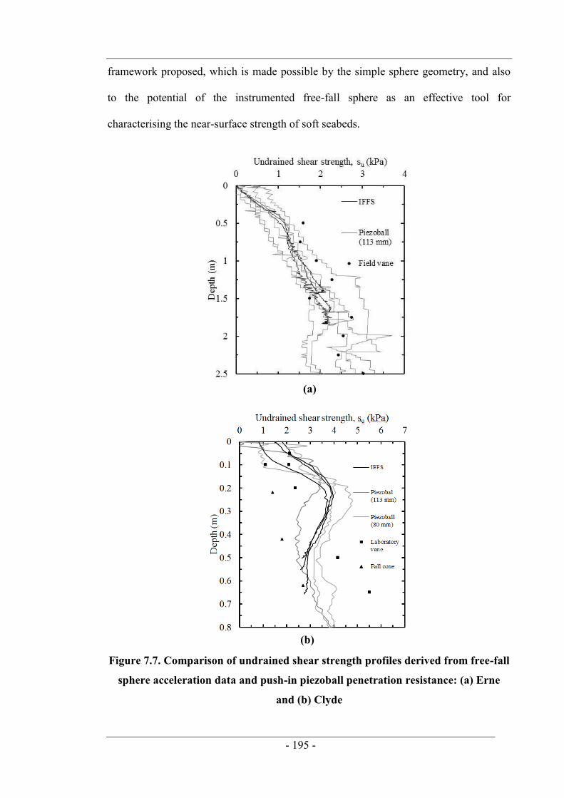
- 195 -
framework proposed, which is made possible by the simple sphere geometry, and also
to the potential of the instrumented free-fall sphere as an effective tool for
characterising the near-surface strength of soft seabeds.
Figure 7.7. Comparison of undrained shear strength profiles derived from free-fall
sphere acceleration data and push-in piezoball penetration resistance: (a) Erne
and (b) Clyde
(a)
(b)
- 196 -
7.9. Conclusions
Acceleration data, measured in field tests where a steel sphere was allowed to free-fall
through water and penetrate the underlying soft soil, have been used in the development
of a theoretical framework that describes the forces acting on a sphere during dynamic
embedment in soil. The framework is cast in terms of both fluid mechanics drag
resistance and geotechnical shear resistance, but formulated in terms of a single capacity
factor that approaches the conventional bearing capacity factor at low strain rates, but
may be up to two orders of magnitude higher when the sphere approaches its terminal
velocity. Experimental data gathered from 87 separate free-fall sphere tests at two sites
are interpreted. The merit of the framework was demonstrated through a simple inverse
analysis in which the undrained shear strength measured during free-fall sphere tests
was calculated from the measured acceleration data, accounting for buoyancy created by
the passage of the advancing sphere and a reduced bearing capacity factor at shallow
embedment. The resulting undrained shear strength profiles were shown to be in
excellent agreement with those derived from piezoball penetrometer tests, indicating the
potential of the free-fall sphere as a simple yet effective tool for characterising the near-
surface strength of soft seabeds.

- 197 -
CHAPTER 8. CENTRIFUGE MODELLING OF AN
INSTRUMENTED FREE-FALL SPHERE FOR
MEASUREMENT OF UNDRAINED STRENGTH IN
FINE-GRAINED SOILS
8.1. Abstract
This paper describes centrifuge tests in which a model free-fall sphere was allowed to
free-fall in water before dynamically embedding within reconstituted samples of kaolin
clay and two offshore natural clays. Instrumentation within the sphere measured
accelerations along three orthogonal axes. The resultant acceleration was used to
calculate sphere velocities and displacements. This allowed the penetration resistance
acting on the sphere to be expressed in terms of a single capacity factor that captures
soil resistance from both shearing and drag, and varies uniquely with the non-
Newtonian Reynolds number. Undrained shear strength profiles obtained from a simple
The final technical chapter extends the experience described in all previous technical
chapters by using the approaches developed in the thesis to further demonstrate the
merit of the IFFS through centrifuge experiments on kaolin clay and two natural soils
offshore soils.
Morton, J. P., O‟Loughlin, C. D. & White. D. J., 2015. Centrifuge modelling of an
instrumented free-fall sphere for measurement of undrained strength in fine grained
soils. Canadian Geotechnical Journal. DOI: 10.1139/cgj-2015-0242.

- 198 -
inverse analysis of the acceleration data show good agreement with those obtained
using conventional push-in penetrometer tests.
8.2. Introduction
Assessments of seabed strength for design are often based on interpretations of the
penetration resistance of a cone, T-bar or ball penetrometer as it is pushed into the soil.
However, this type of test requires a large seabed frame to provide reaction forces to
advance the penetrometer. A more cost effective alternative is to allow a penetrometer
to free-fall through the water column, so that the total energy of the penetrometer at the
seabed mudline provides the force to drive it into the seabed. Experience with such
systems has typically been with slender, shafted projectiles with a conical tip (i.e.
similar to a cone penetrometer). In some cases these devices have flukes near the rear of
the penetrometer for stability during free-fall (e.g. see Figure 8.1). Although the ease
and speed of installation make free-fall penetrometers an attractive option, their
adoption is hampered by difficulties in interpreting soil strength at the very high strain
rates that are prevalent during the dynamic penetration. These strain rates are up to eight
orders of magnitude higher than in a standard laboratory element test. Hydrodynamic
aspects further complicate the analysis. These include drag resistance that not only
occurs during free-fall in water, but also during dynamic embedment in soil, and the
potential for water to become entrained at the projectile-soil interface. The entrainment
of water has been indicated in numerical studies (Sabetamal et al. 2014) and free-fall
penetrometer and anchor field tests (Seifert et al. 2008; Jeanjean et al. 2012). These
complexities present challenges for free-falling penetrometers in firstly, isolating a
value of „dynamic strength‟ from the total resistance experienced by the projectile
during embedment and secondly, scaling this dynamic strength to a „static‟ value
appropriate for design.

- 199 -
In soft fine-grained soils, as an alternative to a free-falling CPT, a spherical free-fall
penetrometer can be used, of the form shown in Figure 8.2 (Morton and O‟Loughlin
2012; Morton et al. 2015). A spherical free-fall penetrometer is attractive as it benefits
from the advantages of full-flow penetrometers, which have more tightly bracketed
bearing capacity factors for deriving the undrained shear strength, su, from the net
penetration resistance (Chung and Randolph 2004). In the context of free-fall
penetrometers, the analysis for a sphere is simpler than for a cone as it does not include
the somewhat complicated frictional resistance that occurs along the shaft of a cone
penetrometer. This resistance is uncertain because it may be affected by water
entrainment (Richardson et al. 2009; Jeanjean et al. 2012) and has been shown to
exhibit different strain-rate dependency compared to the tip (Dayal et al. 1975; Steiner
et al. 2014; Chow et al. 2014). Finally, unlike a cone penetrometer, a sphere may freely
rotate without affecting the projected area and in turn the mobilised shear resistance.
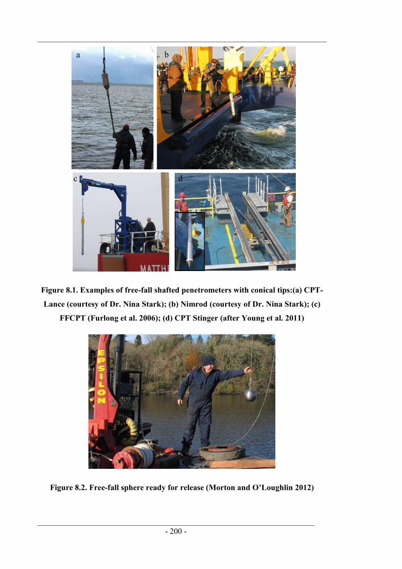
- 200 -
Figure 8.1. Examples of free-fall shafted penetrometers with conical tips:(a) CPT-
Lance (courtesy of Dr. Nina Stark); (b) Nimrod (courtesy of Dr. Nina Stark); (c)
FFCPT (Furlong et al. 2006); (d) CPT Stinger (after Young et al. 2011)
Figure 8.2. Free-fall sphere ready for release (Morton and O’Loughlin 2012)
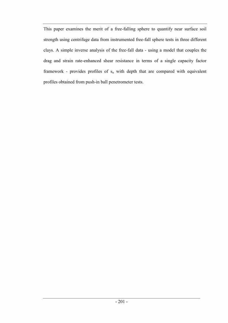
- 201 -
This paper examines the merit of a free-falling sphere to quantify near surface soil
strength using centrifuge data from instrumented free-fall sphere tests in three different
clays. A simple inverse analysis of the free-fall data - using a model that couples the
drag and strain rate-enhanced shear resistance in terms of a single capacity factor
framework - provides profiles of su with depth that are compared with equivalent
profiles obtained from push-in ball penetrometer tests.
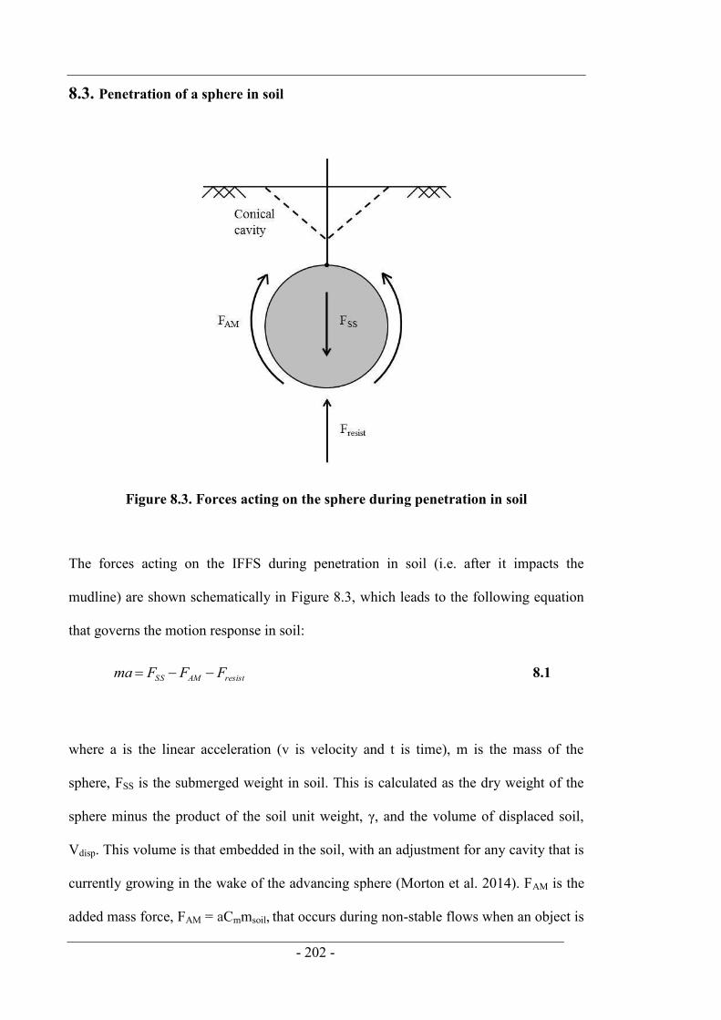
- 202 -
8.3. Penetration of a sphere in soil
Figure 8.3. Forces acting on the sphere during penetration in soil
The forces acting on the IFFS during penetration in soil (i.e. after it impacts the
mudline) are shown schematically in Figure 8.3, which leads to the following equation
that governs the motion response in soil:
resistAMSS FFFma 8.1
where a is the linear acceleration (v is velocity and t is time), m is the mass of the
sphere, FSS is the submerged weight in soil. This is calculated as the dry weight of the
sphere minus the product of the soil unit weight, γ, and the volume of displaced soil,
Vdisp. This volume is that embedded in the soil, with an adjustment for any cavity that is
currently growing in the wake of the advancing sphere (Morton et al. 2014). FAM is the
added mass force, FAM = aCmmsoil, that occurs during non-stable flows when an object is
- 203 -
accelerating or decelerating (Lamb, 1932). The added mass (Cmmsoil) can be interpreted
as the mass of surrounding soil that is accelerated with the sphere, which results in a
force controlled by the added mass coefficient (Cm). The final term on the right hand
side of Equation 8.1 is a combined dynamic resistance force acting on the sphere. Fresist
is conventionally considered as the sum of the strain-rate enhanced bearing resistance,
, and the drag resistance, FD:
2
21 vACAsNFFF pDpopucDsresist opu
8.2
where Nc is a bearing capacity factor, Ap is the projected area of the sphere, su-op is the
mobilised, or operative shear strength at the strain rate relevant to the velocity v, CD is
an drag coefficient and ρ is the density of the soil. However, Sadhi et al. (2014) and
Morton et al. (2015) showed that these terms can be combined via a superposition
approach in which the strength and drag resistance components are expressed as a single
resistance force:
popuresist ANsF 8.3
where N is a geometry-dependant capacity factor that is dependent on the non-
Newtonian Reynolds number, Renon-Newtonian, (Zakeri et al. 2008):
opuNewtoniannon s
v
,
2
Re 8.4
- 204 -
The well know influence of strain rate, on the mobilised strength due to viscous
effects is described by a power law enhancement of the soil strength (Briaud et al.,
1984; Biscontin and Pestana, 2001; Peuchen and Mayne, 2007; Jeong et al., 2009;
Lehane et al. 2009; O‟Loughlin et al. 2013b):
refrefuopu ss
,, 8.5
where su,ref is the undrained shear strength at the reference strain rate ref and β is a strain
rate parameter defining the strength of the rate effect for any given soil. As shown by
Lehane et al. 2009, O‟Loughlin et al. (2013b) and Chow et al. (2014), the operational
shear strain rate around a penetrometer may be approximated by v/D, such that Equation
8.5 may be written as:
refrefuopu Dv
Dvss//
, 8.6
It follows from Equations 8.2, 8.3 and 8.4 that a relationship between N and Renon-
Newtonian may then be expressed as:
cNewtoniannonD NCN Re21 8.7
Morton et al. (2015) showed that this framework is capable of describing the resistance
acting on a sphere as measured in field tests with an IFFS. The model requires three
main input parameters: the drag coefficient, CD, for the sphere over the range of non-
Newtonian Reynolds numbers applicable to dynamic penetration in soil, the strain rate
- 205 -
parameter, β, and a reference strain rate, ref. The selection of these parameters are
considered later in the paper.
Equation 8.7 also requires an assessment of the bearing capacity factor, Nc, and its
evolution with depth, as for push-in penetrometer tests such as the CPT, T-bar or ball.
Hossain et al. (2005), White et al. (2010), Tho et al. (2012) and Morton et al. (2014)
showed that this evolution depends on the dimensionless soil strength ratio, su/γ'D,
where γ' is the effective unit weight of the soil and D is the diameter of the penetrating
body. The transition from a reduced Nc value at shallow penetration where the failure
mechanism extends to the soil surface, to the limiting value for deep embedment
associated with a full-flow mechanism, has recently been investigated for a sphere over
a wide range of su/γ'D (Morton et al. 2014). This approach, expressed by the following
power function, has also been shown to work well in two other natural soils (Morton et
al. 2015):
p
opdeep
opdeepbc w
wNN
ˆˆ
8.8
where the transitional depth at which Nc = Nc-deep is given by:
f
u
cu
opdeep
eD
s
adD
sbaw
/1
ˆ
8.9
and the fitting constants a = 16.3, b = 0.12, c = 1.3, d = 0.52, e = 4.9, f = 1.5 and p =
0.49.
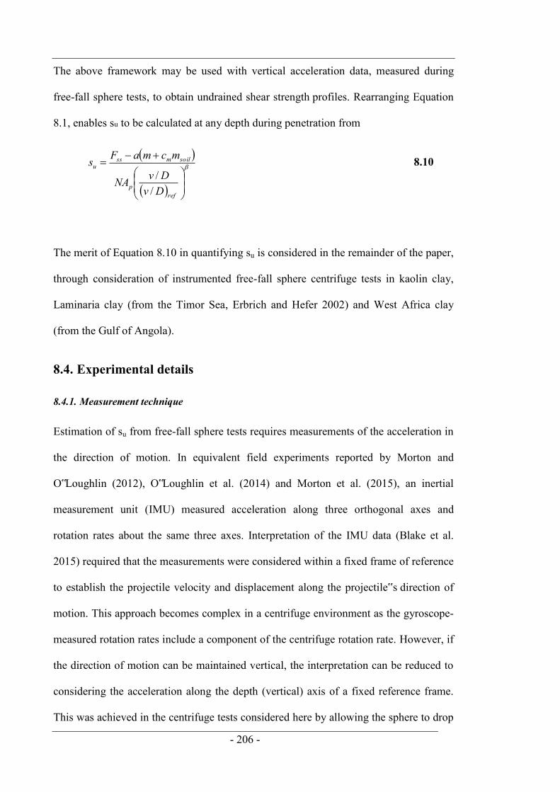
- 206 -
The above framework may be used with vertical acceleration data, measured during
free-fall sphere tests, to obtain undrained shear strength profiles. Rearranging Equation
8.1, enables su to be calculated at any depth during penetration from
refp
soilmssu
DvDvNA
mcmaFs
//
8.10
The merit of Equation 8.10 in quantifying su is considered in the remainder of the paper,
through consideration of instrumented free-fall sphere centrifuge tests in kaolin clay,
Laminaria clay (from the Timor Sea, Erbrich and Hefer 2002) and West Africa clay
(from the Gulf of Angola).
8.4. Experimental details
8.4.1. Measurement technique
Estimation of su from free-fall sphere tests requires measurements of the acceleration in
the direction of motion. In equivalent field experiments reported by Morton and
O‟Loughlin (2012), O‟Loughlin et al. (2014) and Morton et al. (2015), an inertial
measurement unit (IMU) measured acceleration along three orthogonal axes and
rotation rates about the same three axes. Interpretation of the IMU data (Blake et al.
2015) required that the measurements were considered within a fixed frame of reference
to establish the projectile velocity and displacement along the projectile‟s direction of
motion. This approach becomes complex in a centrifuge environment as the gyroscope-
measured rotation rates include a component of the centrifuge rotation rate. However, if
the direction of motion can be maintained vertical, the interpretation can be reduced to
considering the acceleration along the depth (vertical) axis of a fixed reference frame.
This was achieved in the centrifuge tests considered here by allowing the sphere to drop
- 207 -
through a vertical installation guide located above the soil surface. The acceleration
along the vertical direction of motion can then be determined from the resultant
acceleration calculated from the acceleration components measured along the three
orthogonal axes shown in Figure 8.4a using a tri-axis accelerometer.
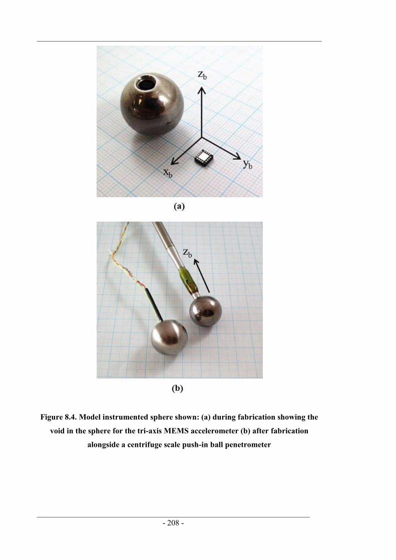
- 208 -
Figure 8.4. Model instrumented sphere shown: (a) during fabrication showing the
void in the sphere for the tri-axis MEMS accelerometer (b) after fabrication
alongside a centrifuge scale push-in ball penetrometer

- 209 -
8.4.2. Instrumented free-fall sphere
The 20 mm diameter stainless steel sphere used for the free-fall centrifuge experiments
(see Figure 8.4) had a mass of 31 grams. The centrifuge tests were conducted at 12.5 g,
such that the centrifuge model IFFS is equivalent to the 250 mm IFFS used in the field
trials referred to previously and shown in Figure 8.3. The model sphere was
instrumented with a tri-axis ADXL377 +/- 200 g MEMS accelerometer, measuring
approximately 5 × 5 × 2 mm. A commercially-available ±200 g accelerometer was
chosen as the only device offering three-axis sensing within the size constraints, and
providing an analogue output. The sensor was located within a cylindrical void in the
sphere (see Figure 8.4a) that was subsequently filled with epoxy. The accelerometer was
aligned with the body frame of the sphere as shown in Figure 8.4a. The body frame is a
reference frame with three orthogonal axes xb, yb and zb. Before release in the centrifuge
tests, the sphere was oriented such that the zb axis was approximately parallel to the
centripetal acceleration vector in the centrifuge. The accelerometer measures
accelerations Abx, Aby and Abz along the three orthogonal axes of the body reference
frame. As discussed previously, these data are used to calculate the resultant
acceleration, Ar:
222bzbybxr AAAA 8.11
The linear acceleration, a, of the sphere then becomes:
rAa r2 8.12
where ω is the angular velocity of the centrifuge and ω2r is the centripetal acceleration
level at a distance, r, from the centrifuge‟s axis of rotation to the sphere location.

- 210 -
8.4.3. Soil preparation technique
The offshore clay samples were reconstituted by adding minimal amounts of water to
reconstitute the soils as slurries and the kaolin clay sample was prepared by mixing
kaolin powder with water to form a slurry at a moisture content of 120%. The slurries
were then mixed continuously for about 24 hours and then transferred to sample boxes,
each with internal dimensions 598 mm long, 117 mm wide and 300 mm deep. These
three sample boxes were then nested side by side in a larger strongbox to allow „in-
flight‟ consolidation of the three samples at the same time. The acceleration field acts
radially in the centrifuge so the testing was performed only with the sample located
along the longitudinal centreline of the beam centrifuge strongbox. Using three
narrower internal sample boxes facilitated a greater test plan area by interchanging the
sample boxes to put the „test box‟ in the middle.
A 10 mm layer of sand was placed at the base of each box (i.e. before pouring the
slurry) and the end walls of each box were then lined with a drainage blanket to ensure
that there was no hydraulic gradient between the top and base of the sample. The
samples were normally consolidated under self-weight consolidation in the centrifuge at
12.5 g for approximately 14 days, during which time a 30 mm water layer was
maintained at the sample surface to ensure saturation. After consolidation, the surface of
each soil sample was scraped to create a slightly overconsolidated soil with a level
surface and final sample heights of 225 mm for the kaolin and West Africa Clay and
160 mm for the Laminaria clay.
8.4.4. Centrifuge test details and procedures
The centrifuge test programme included a combination of free-fall sphere tests and
constant rate of penetration ball and T-bar penetrometer tests to determine the reference
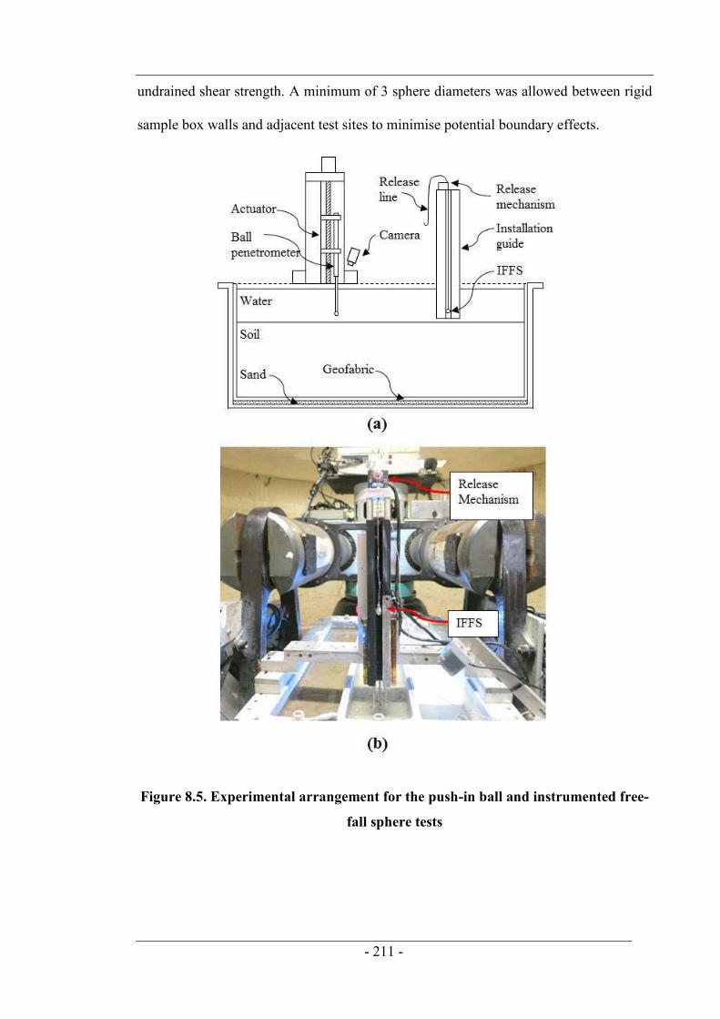
- 211 -
undrained shear strength. A minimum of 3 sphere diameters was allowed between rigid
sample box walls and adjacent test sites to minimise potential boundary effects.
Figure 8.5. Experimental arrangement for the push-in ball and instrumented free-
fall sphere tests
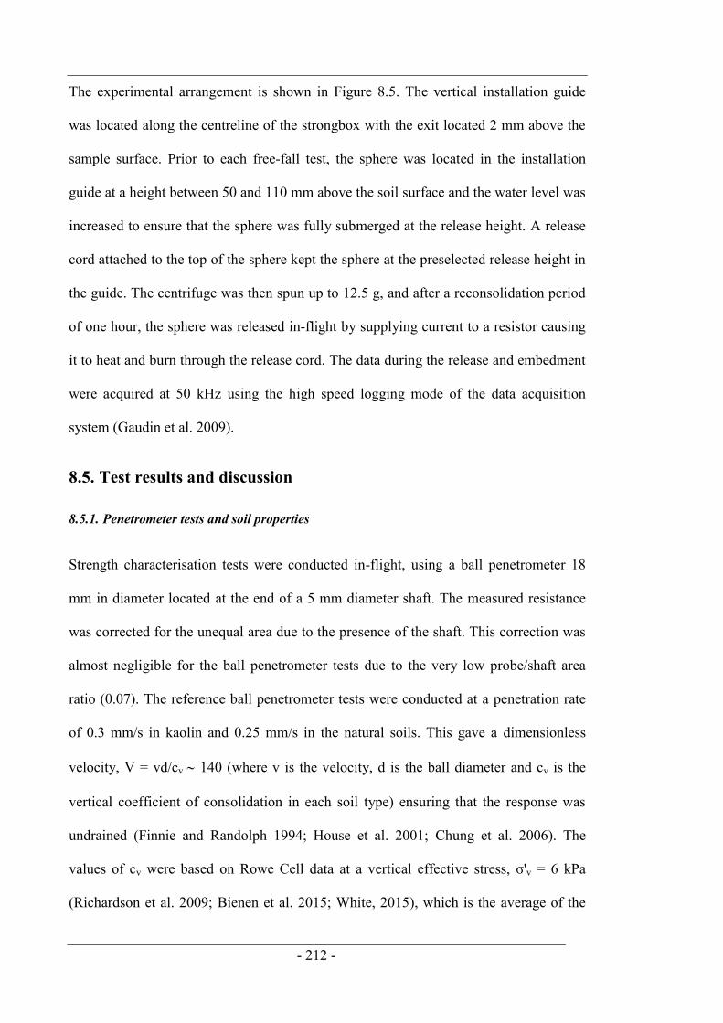
- 212 -
The experimental arrangement is shown in Figure 8.5. The vertical installation guide
was located along the centreline of the strongbox with the exit located 2 mm above the
sample surface. Prior to each free-fall test, the sphere was located in the installation
guide at a height between 50 and 110 mm above the soil surface and the water level was
increased to ensure that the sphere was fully submerged at the release height. A release
cord attached to the top of the sphere kept the sphere at the preselected release height in
the guide. The centrifuge was then spun up to 12.5 g, and after a reconsolidation period
of one hour, the sphere was released in-flight by supplying current to a resistor causing
it to heat and burn through the release cord. The data during the release and embedment
were acquired at 50 kHz using the high speed logging mode of the data acquisition
system (Gaudin et al. 2009).
8.5. Test results and discussion
8.5.1. Penetrometer tests and soil properties
Strength characterisation tests were conducted in-flight, using a ball penetrometer 18
mm in diameter located at the end of a 5 mm diameter shaft. The measured resistance
was corrected for the unequal area due to the presence of the shaft. This correction was
almost negligible for the ball penetrometer tests due to the very low probe/shaft area
ratio (0.07). The reference ball penetrometer tests were conducted at a penetration rate
of 0.3 mm/s in kaolin and 0.25 mm/s in the natural soils. This gave a dimensionless
velocity, V = vd/cv 140 (where v is the velocity, d is the ball diameter and cv is the
vertical coefficient of consolidation in each soil type) ensuring that the response was
undrained (Finnie and Randolph 1994; House et al. 2001; Chung et al. 2006). The
values of cv were based on Rowe Cell data at a vertical effective stress, σ'v = 6 kPa
(Richardson et al. 2009; Bienen et al. 2015; White, 2015), which is the average of the
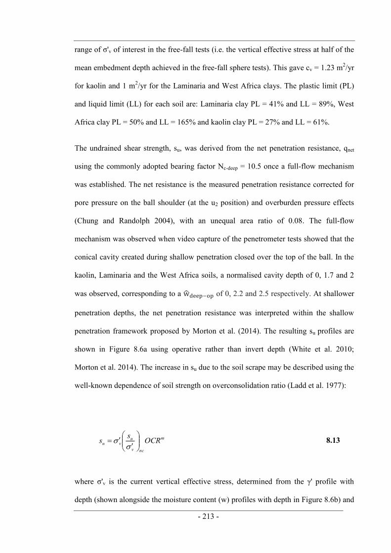
- 213 -
range of σ'v of interest in the free-fall tests (i.e. the vertical effective stress at half of the
mean embedment depth achieved in the free-fall sphere tests). This gave cv = 1.23 m2/yr
for kaolin and 1 m2/yr for the Laminaria and West Africa clays. The plastic limit (PL)
and liquid limit (LL) for each soil are: Laminaria clay PL = 41% and LL = 89%, West
Africa clay PL = 50% and LL = 165% and kaolin clay PL = 27% and LL = 61%.
The undrained shear strength, su, was derived from the net penetration resistance, qnet
using the commonly adopted bearing factor Nc-deep = 10.5 once a full-flow mechanism
was established. The net resistance is the measured penetration resistance corrected for
pore pressure on the ball shoulder (at the u2 position) and overburden pressure effects
(Chung and Randolph 2004), with an unequal area ratio of 0.08. The full-flow
mechanism was observed when video capture of the penetrometer tests showed that the
conical cavity created during shallow penetration closed over the top of the ball. In the
kaolin, Laminaria and the West Africa soils, a normalised cavity depth of 0, 1.7 and 2
was observed, corresponding to a of 0, 2.2 and 2.5 respectively. At shallower
penetration depths, the net penetration resistance was interpreted within the shallow
penetration framework proposed by Morton et al. (2014). The resulting su profiles are
shown in Figure 8.6a using operative rather than invert depth (White et al. 2010;
Morton et al. 2014). The increase in su due to the soil scrape may be described using the
well-known dependence of soil strength on overconsolidation ratio (Ladd et al. 1977):
m
ncv
uvu OCRss
8.13
where σ'v is the current vertical effective stress, determined from the γ' profile with
depth (shown alongside the moisture content (w) profiles with depth in Figure 8.6b) and

- 214 -
the slightly varying acceleration level with radius within the centrifuge (12.5 to 13.7 g
over the depth of penetration in soil), m is the plastic volumetric strain ratio (Schofield
and Wroth 1968) taken as m = 0.8.

- 215 -
Figure 8.6. Profiles of: (a) undrained shear strength with depth (from ball
penetrometer tests) and (b) moisture content and effective unit weight with depth
established from post-testing sample cores
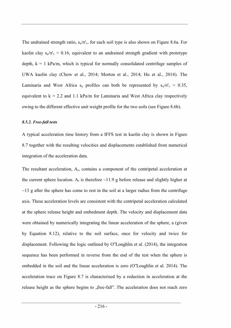
- 216 -
The undrained strength ratio, su/σ'v, for each soil type is also shown on Figure 8.6a. For
kaolin clay su/σ'v = 0.16, equivalent to an undrained strength gradient with prototype
depth, k = 1 kPa/m, which is typical for normally consolidated centrifuge samples of
UWA kaolin clay (Chow et al., 2014; Morton et al., 2014; Hu et al., 2014). The
Laminaria and West Africa su profiles can both be represented by su/σ'v = 0.35,
equivalent to k = 2.2 and 1.1 kPa/m for Laminaria and West Africa clay respectively
owing to the different effective unit weight profile for the two soils (see Figure 8.6b).
8.5.2. Free-fall tests
A typical acceleration time history from a IFFS test in kaolin clay is shown in Figure
8.7 together with the resulting velocities and displacements established from numerical
integration of the acceleration data.
The resultant acceleration, Ar, contains a component of the centripetal acceleration at
the current sphere location. Ar is therefore ~11.9 g before release and slightly higher at
~13 g after the sphere has come to rest in the soil at a larger radius from the centrifuge
axis. These acceleration levels are consistent with the centripetal acceleration calculated
at the sphere release height and embedment depth. The velocity and displacement data
were obtained by numerically integrating the linear acceleration of the sphere, a (given
by Equation 8.12), relative to the soil surface, once for velocity and twice for
displacement. Following the logic outlined by O‟Loughlin et al. (2014), the integration
sequence has been performed in reverse from the end of the test when the sphere is
embedded in the soil and the linear acceleration is zero (O‟Loughlin et al. 2014). The
acceleration trace on Figure 8.7 is characterised by a reduction in acceleration at the
release height as the sphere begins to „free-fall‟. The acceleration does not reach zero
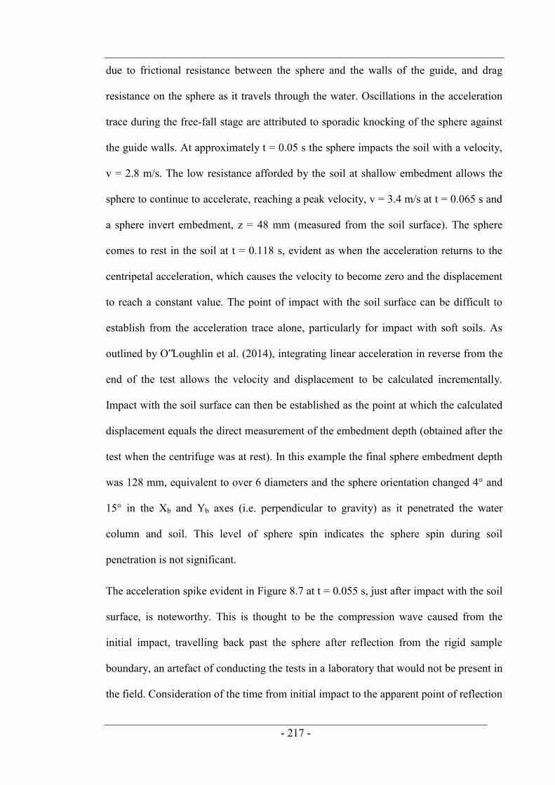
- 217 -
due to frictional resistance between the sphere and the walls of the guide, and drag
resistance on the sphere as it travels through the water. Oscillations in the acceleration
trace during the free-fall stage are attributed to sporadic knocking of the sphere against
the guide walls. At approximately t = 0.05 s the sphere impacts the soil with a velocity,
v = 2.8 m/s. The low resistance afforded by the soil at shallow embedment allows the
sphere to continue to accelerate, reaching a peak velocity, v = 3.4 m/s at t = 0.065 s and
a sphere invert embedment, z = 48 mm (measured from the soil surface). The sphere
comes to rest in the soil at t = 0.118 s, evident as when the acceleration returns to the
centripetal acceleration, which causes the velocity to become zero and the displacement
to reach a constant value. The point of impact with the soil surface can be difficult to
establish from the acceleration trace alone, particularly for impact with soft soils. As
outlined by O‟Loughlin et al. (2014), integrating linear acceleration in reverse from the
end of the test allows the velocity and displacement to be calculated incrementally.
Impact with the soil surface can then be established as the point at which the calculated
displacement equals the direct measurement of the embedment depth (obtained after the
test when the centrifuge was at rest). In this example the final sphere embedment depth
was 128 mm, equivalent to over 6 diameters and the sphere orientation changed 4° and
15° in the Xb and Yb axes (i.e. perpendicular to gravity) as it penetrated the water
column and soil. This level of sphere spin indicates the sphere spin during soil
penetration is not significant.
The acceleration spike evident in Figure 8.7 at t = 0.055 s, just after impact with the soil
surface, is noteworthy. This is thought to be the compression wave caused from the
initial impact, travelling back past the sphere after reflection from the rigid sample
boundary, an artefact of conducting the tests in a laboratory that would not be present in
the field. Consideration of the time from initial impact to the apparent point of reflection
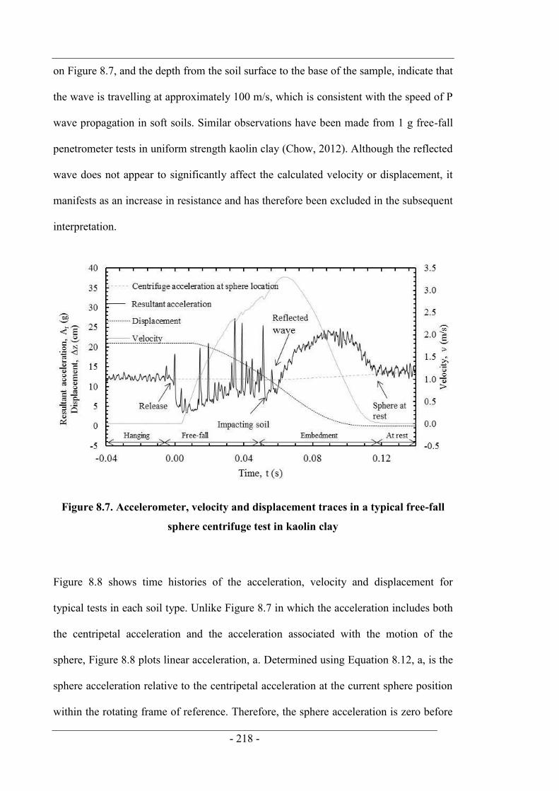
- 218 -
on Figure 8.7, and the depth from the soil surface to the base of the sample, indicate that
the wave is travelling at approximately 100 m/s, which is consistent with the speed of P
wave propagation in soft soils. Similar observations have been made from 1 g free-fall
penetrometer tests in uniform strength kaolin clay (Chow, 2012). Although the reflected
wave does not appear to significantly affect the calculated velocity or displacement, it
manifests as an increase in resistance and has therefore been excluded in the subsequent
interpretation.
Figure 8.7. Accelerometer, velocity and displacement traces in a typical free-fall
sphere centrifuge test in kaolin clay
Figure 8.8 shows time histories of the acceleration, velocity and displacement for
typical tests in each soil type. Unlike Figure 8.7 in which the acceleration includes both
the centripetal acceleration and the acceleration associated with the motion of the
sphere, Figure 8.8 plots linear acceleration, a. Determined using Equation 8.12, a, is the
sphere acceleration relative to the centripetal acceleration at the current sphere position
within the rotating frame of reference. Therefore, the sphere acceleration is zero before
- 219 -
release, changing abruptly to about 8g immediately after release (consistent with the
centripetal acceleration at the sphere release height) and zero when the sphere has come
to rest in the soil.
Velocity and displacement traces derived from the linear acceleration data are provided
in Figure 8.8b and Figure 8.8c respectively.
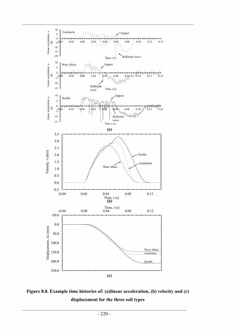
- 220 -
Figure 8.8. Example time histories of: (a)linear acceleration, (b) velocity and (c)
displacement for the three soil types
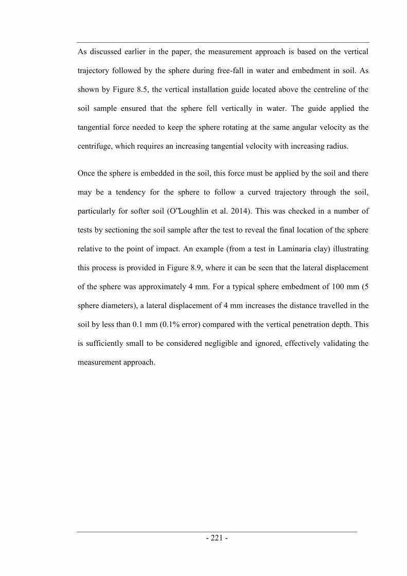
- 221 -
As discussed earlier in the paper, the measurement approach is based on the vertical
trajectory followed by the sphere during free-fall in water and embedment in soil. As
shown by Figure 8.5, the vertical installation guide located above the centreline of the
soil sample ensured that the sphere fell vertically in water. The guide applied the
tangential force needed to keep the sphere rotating at the same angular velocity as the
centrifuge, which requires an increasing tangential velocity with increasing radius.
Once the sphere is embedded in the soil, this force must be applied by the soil and there
may be a tendency for the sphere to follow a curved trajectory through the soil,
particularly for softer soil (O‟Loughlin et al. 2014). This was checked in a number of
tests by sectioning the soil sample after the test to reveal the final location of the sphere
relative to the point of impact. An example (from a test in Laminaria clay) illustrating
this process is provided in Figure 8.9, where it can be seen that the lateral displacement
of the sphere was approximately 4 mm. For a typical sphere embedment of 100 mm (5
sphere diameters), a lateral displacement of 4 mm increases the distance travelled in the
soil by less than 0.1 mm (0.1% error) compared with the vertical penetration depth. This
is sufficiently small to be considered negligible and ignored, effectively validating the
measurement approach.

- 222 -
Figure 8.9. Post-test analysis of the sphere trajectory and measurement of the final
embedment depth
8.5.3. Interpretation of free-fall acceleration data
The acceleration data are now considered within the simple framework outlined earlier
in the paper that accounts for both geotechnical shearing resistance and fluid mechanics
drag resistance. Rearranging Equation 8.7 allows N to be established as a function of
Renon-Newtonian. This is shown on Figure 8.9a, b and c for the Laminaria, West Africa and
kaolin clays respectively. The highest values of Renon-Newtonian correspond with initial
penetration, where the soil strength is low and the sphere velocity is high. Differences in
the maximum Renon-Newtonian values in Figure 8.9 reflects differences in strength and
impact velocities between tests in each soil. At these high values of Renon-Newtonian, N is
typically between 20 and 300, 2 to 30 times higher than the (geotechnical) bearing
capacity factor, Nc. As penetration progresses, Renon-Newtonian reduces as the soil strength
increases (as reflected in Figure 8.6a) and the sphere velocity reduces. This has the
effect of decreasing the dynamic resistance component, resulting in reducing values of
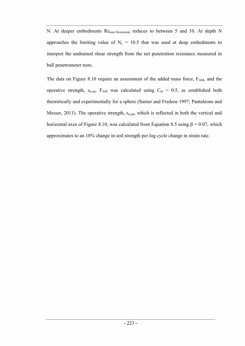
- 223 -
N. At deeper embedments Renon-Newtonian reduces to between 5 and 10. At depth N
approaches the limiting value of Nc = 10.5 that was used at deep embedments to
interpret the undrained shear strength from the net penetration resistance measured in
ball penetrometer tests.
The data on Figure 8.10 require an assessment of the added mass force, FAM, and the
operative strength, su,op. FAM was calculated using Cm = 0.5, as established both
theoretically and experimentally for a sphere (Sumer and Fredsoe 1997; Pantaleone and
Messer, 2011). The operative strength, su,op, which is reflected in both the vertical and
horizontal axes of Figure 8.10, was calculated from Equation 8.5 using β = 0.07, which
approximates to an 18% change in soil strength per log cycle change in strain rate.

- 224 -
Figure 8.10. Relationship between N and Renon-Newtonian for a sphere in the three soil
types: (a) Laminaria soil (b) West Africa clay (c) kaolin
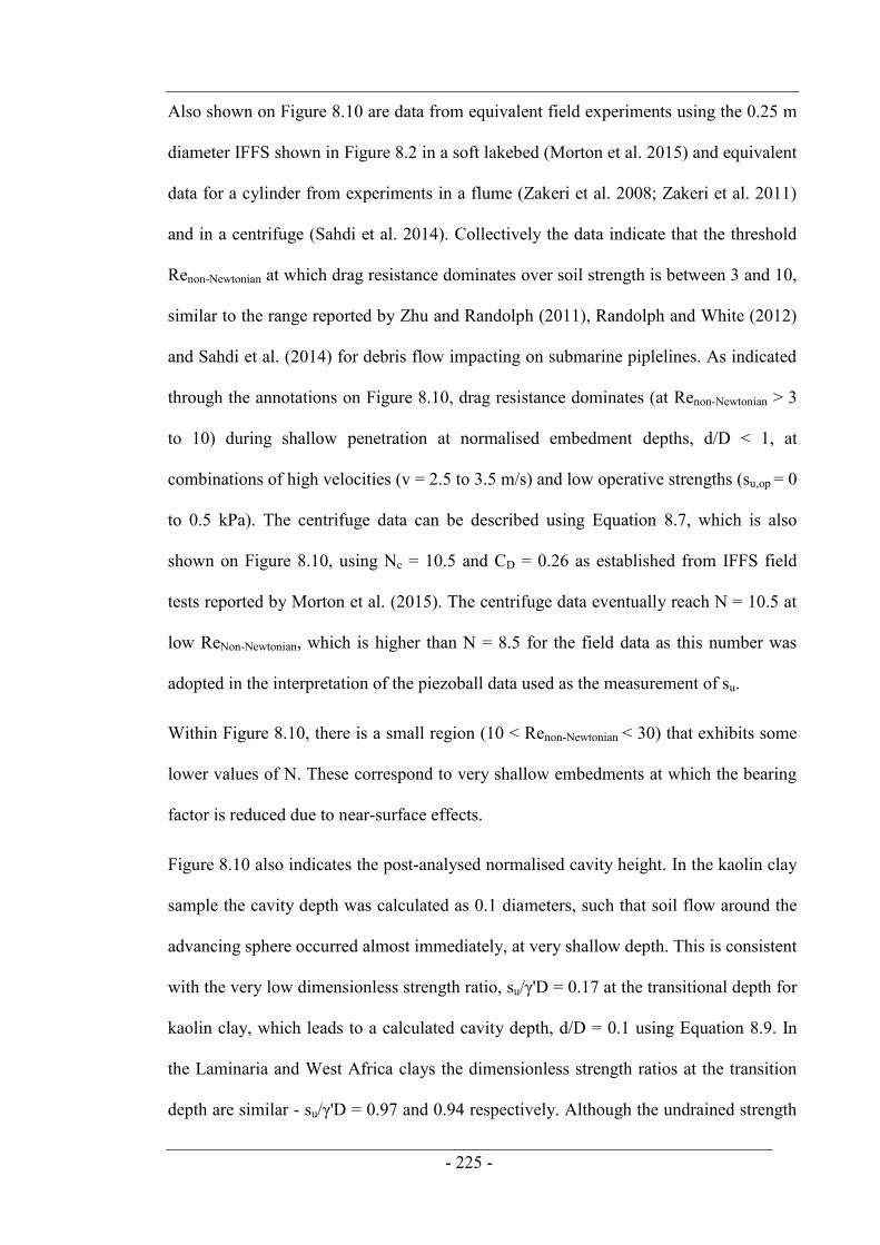
- 225 -
Also shown on Figure 8.10 are data from equivalent field experiments using the 0.25 m
diameter IFFS shown in Figure 8.2 in a soft lakebed (Morton et al. 2015) and equivalent
data for a cylinder from experiments in a flume (Zakeri et al. 2008; Zakeri et al. 2011)
and in a centrifuge (Sahdi et al. 2014). Collectively the data indicate that the threshold
Renon-Newtonian at which drag resistance dominates over soil strength is between 3 and 10,
similar to the range reported by Zhu and Randolph (2011), Randolph and White (2012)
and Sahdi et al. (2014) for debris flow impacting on submarine piplelines. As indicated
through the annotations on Figure 8.10, drag resistance dominates (at Renon-Newtonian > 3
to 10) during shallow penetration at normalised embedment depths, d/D < 1, at
combinations of high velocities (v = 2.5 to 3.5 m/s) and low operative strengths (su,op = 0
to 0.5 kPa). The centrifuge data can be described using Equation 8.7, which is also
shown on Figure 8.10, using Nc = 10.5 and CD = 0.26 as established from IFFS field
tests reported by Morton et al. (2015). The centrifuge data eventually reach N = 10.5 at
low ReNon-Newtonian, which is higher than N = 8.5 for the field data as this number was
adopted in the interpretation of the piezoball data used as the measurement of su.
Within Figure 8.10, there is a small region (10 < Renon-Newtonian < 30) that exhibits some
lower values of N. These correspond to very shallow embedments at which the bearing
factor is reduced due to near-surface effects.
Figure 8.10 also indicates the post-analysed normalised cavity height. In the kaolin clay
sample the cavity depth was calculated as 0.1 diameters, such that soil flow around the
advancing sphere occurred almost immediately, at very shallow depth. This is consistent
with the very low dimensionless strength ratio, su/γ'D = 0.17 at the transitional depth for
kaolin clay, which leads to a calculated cavity depth, d/D = 0.1 using Equation 8.9. In
the Laminaria and West Africa clays the dimensionless strength ratios at the transition
depth are similar - su/γ'D = 0.97 and 0.94 respectively. Although the undrained strength

- 226 -
profiles for the Laminaria and West Africa clays differs by a factor of approximately 2,
the lower effective unit weight of the Laminaria clay results in almost identical
dimensionless strength ratios for the two soils. Although this results in deeper cavities
for the tests in Laminaria and West Africa clays, calculated using Equation 8.9 as
= 2.0 and 2.3 for Laminaria and West Africa clay respectively. In both soils
the sphere penetrated beyond the cavity depth such that a full-flow failure mechanism
was established.
The merit of the framework is now explored by using the linear, acceleration described
in Equation 8.12 to obtain su profiles for each soil, based on the dynamic free fall data.
In kaolin, a deeply embedment soil flow mechanism is assumed, such that the
submerged weight of the sphere, FSS, is the weight of the sphere in water minus the
effective weight of the displaced soil, which may be calculated using the volume of the
sphere. The capacity factor, N, may then be determined using Equation 8.7 with Nc =
10.5 and CD = 0.26. As discussed in the previous section, su/γ'D ~ 0.95 is higher in the
West Africa and Laminaria clays at the final sphere embedment depth, which is
sufficiently high that both the variation in Nc with embedment depth and the soil
buoyancy associated with the cavity formed by the penetrating sphere require
consideration (Morton et al. 2014). The transitional embedment depth at which Nc = Nc-
deep calculated using Equation 8.9 compared well to the post-analysed which
were 2.2 and 2.5 for Laminaria and West Africa clay respectively and were within 10%
of the calculated measurements. These transitional embedment depths allow the
variation in Nc with depth to be determined using Equation 8.8.
The resulting su profiles obtained from Equation 8.10 are compared with the push-in ball
penetrometer profiles in Figure 8.11 using operative rather than invert depth (White et
al. 2010; Morton et al. 2014). Shallow embedment effects have been considered in the

- 227 -
same way for the push-in tests as the free-fall tests. Interruptions to the su profiles on
Figure 8.11 correspond with the acceleration spikes observed in Figure 8.8 that are
attributed to compression wave reflections and have been removed before conducting
the inverse analysis. Figure 8.11 shows good agreement between the push-in and free-
fall su profiles, despite some disparity at very shallow embedment. The level of
agreement observed on Figure 8.8 confirms the merit of the interpretation framework,
which is made possible by the simple sphere geometry, and also to the potential of the
free-fall sphere to be used as an effective tool for characterising the near-surface
strength of soft seabeds. As discussed previously, the framework extends the
interpretation of a push-in ball penetrometer test using only two additional geotechnical
parameters, CD and β.
The value of CD for a bluff body depends on the flow regime and the object geometry,
as is well established in fluid mechanics. For a sphere, CD does not vary significantly
over the range of non-Newtonian Reynolds numbers in Figure 8.10 where drag is
significant (Schlichting et al. 2000). The consistent scatter around the trend line in
Figure 8.10 indicates that a more refined approach with CD varying with Renon-Newtonian
would not capture the data set any better.
The range of β reported in the literature is quite wide, spanning β = 0.05 to 0.17 (Jeong
et al. 2009), and a choice of is required in the interpretation of dynamic penetration
problems. The wide reported range is partly due to different strain rate ranges being
considered and a variety of test conditions, both in situ and in a laboratory. For instance,
laboratory element tests involving variable strain rates tend to be at relatively low strain
rates (typically 1%/h or 2.8 × 10⁻⁶ s-1; Boukpeti et al. 2012) and measure intact strength
with no strength reduction from softening. In contrast, variable rate full-flow
penetrometer tests usually involve strain rates in the range 0.2 to 20 s-1 and include

- 228 -
compensating effects of strain softening that limit the strength increases associated with
increasing strain rates. IFFS tests include a similar degree of strain softening to a
variable rate full-flow penetrometer test. They also only involve slightly greater strain
rates because the increased velocity is partly compensated by the larger diameter
(maximum v/D = 31 and 130 s-1 for field and centrifuge free fall ball tests respectively).
Therefore, β values for an IFFS test should be guided by those measured in variable rate
full-flow penetrometer tests, which typically give β = 0.05 to 0.09 (Low et al. 2008;
Chung et al. 2006). The effect of adjusting β over this range is explored in Figure 8.12
for Laminaria clay. It is apparent that the lower bound β = 0.05 corresponds with the
largest departure from the base case profile established using β = 0.07, although by less
than 20%. This uncertainty is comparable to the differences that are commonly linked to
uncertainty between different laboratory strength tests (Bienen et al. 2010).
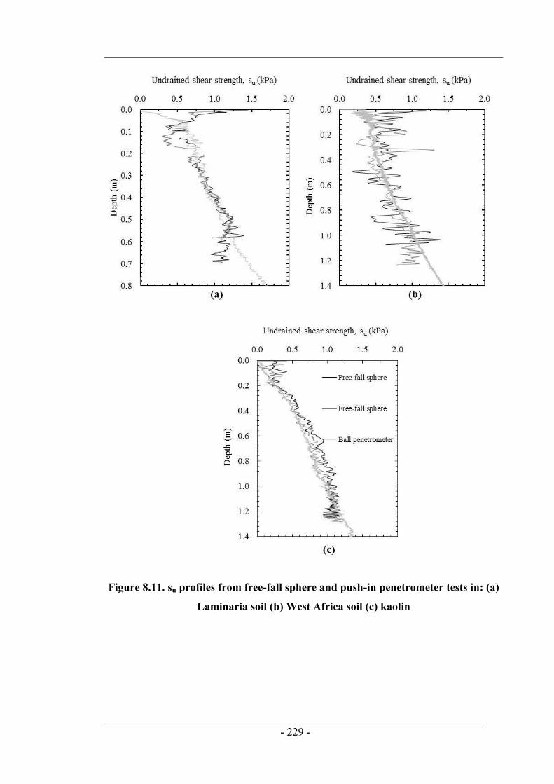
- 229 -
Figure 8.11. su profiles from free-fall sphere and push-in penetrometer tests in: (a)
Laminaria soil (b) West Africa soil (c) kaolin

- 230 -
Figure 8.12. Effect of varying β parameter on free-fall sphere su profile
8.6. Conclusion
This paper has presented centrifuge tests undertaken to investigate the potential for a
new in situ tool – the Instrumented Free-Fall Sphere (IFFS) – to measure the undrained
shear strength profile of soft soil. The centrifuge experiments, which were conducted in
kaolin clay and two reconstituted offshore clays, from Laminaria (Timor Sea) and West
Africa (Gulf of Guinea) clay gave sphere embedments that were up to 5.5 diameters,
which would provide strength measurements over the upper 1.5 m of the seabed for a
practically-dimensioned field tool.
Interpretation of sphere acceleration measurements to quantify the soil strength relied
on a framework cast in terms of both drag resistance and geotechnical shear resistance,
but formulated in terms of a single capacity factor. This capacity factor reduces to the

- 231 -
conventional geotechnical bearing capacity factor at low strain rates, but has been
shown in these experiments to be over an order of magnitude larger when the sphere is
penetrating at high velocities.
The merit of the simple framework was demonstrated through an inverse analysis in
which the undrained shear strength was calculated from the measured acceleration data,
accounting for buoyancy created by the passage of the advancing sphere and a reduced
bearing capacity factor at shallow embedment. Good agreement was obtained between
the dynamically measured su profile and the su profile measured during push-in ball
penetrometer tests. The level of agreement shown, and the relative insensitivity to the
choice of strain rate parameter, suggests that the IFFS is an effective tool for
characterising the near-surface strength of soft seabeds. This is in part due to the fact
that the IFFS, unlike a slender FFP, requires no correction for shaft effects and the
associated strain rate difficulties. Given the positive research findings, it is desired that
future experiments would extend the validation of dynamic versus static su data to a
wider range of soils and focus on practical aspects of deployment and recovery of the
device. Another option that is of interest is the optimization of size and weight of the
IFFS for various soils types, potentially creating an „IFFS family‟ for different expected
soil conditions.
- 232 -
CHAPTER 9. CONCLUSIONS
9.1. Summary
This thesis has introduced a new free-falling penetrometer as a cost effective and
accurate in situ site investigation tool. The new penetrometer is spherical in design and
comprises instrumentation to capture the motion history of the sphere during free-fall in
water and penetration in soil. The Instrumented Free-Fall Sphere (IFFS) represents a
step-change in free-falling penetrometer design, departing from the traditional slender
full-shafted projectile geometry. The IFFS combines the benefits of free-falling
penetrometers with the advantages of full-flow penetrometers which can more
accurately derive the undrained shear strength, su. This is primarily because: (a) it is
unnecessary to eliminate or correct for the shaft resistance in order to directly infer the
soil strength from the bearing resistance, and (b) there is greater uncertainty associated
with shaft resistance rate effects than bearing resistance. It is envisaged that significant
cost savings could be realised by utilising the IFFS in conjunction with other projects,
such as geophysical surveys that typically occur earlier in the site investigation
campaign. This is made possible due to the ease and speed of operation and the
potential to deploy the IFFS from smaller vessels, relative to the conventional approach
of using push-in penetrometers that require larger vessels and seabed frames.
The thesis primarily focused on assessing the viability of the new penetrometer design
by carrying out an experimental study through field tests and centrifuge experiments.
The field tests were conducted on a 0.25 m diameter IFFS in two locations: (i) an inland
- 233 -
lake, Lower Lough Erne in the Northwest of Ireland and (ii) an offshore site in the Firth
of Clyde which is located off the coast of Scotland in the Irish Sea. The sphere was
instrumented with a custom-made, low cost, 6 degree of freedom (6DoF) inertial
measurement unit (IMU) to measure the sphere acceleration and associated velocity and
displacement. The initial field tests provided the „proof of concept‟ and provided a basis
for understanding the behaviour during free-fall in water and dynamic embedment in
soil.
The centrifuge experiments were carried out in two phases - the first focussing on the
shallow penetration effects of an 11.3 mm diameter ball penetrometer (investigated in
Chapter 4). Shallow penetration effects alter the relationship between penetration
resistance and undrained shear strength. If ignored, they can lead to an under-estimation
of the undrained shear strength in the near surface soil. A series of formulations were
proposed to determine more accurately the undrained shear strength of near surface soil
over the range of dimensionless strength ratios that are of interest to offshore
applications.
The second phase of centrifuge testing focussed on the dynamic embedment of 20 mm
diameter model IFFS in three different soils: (i) Laminaria soil recovered from the
Timor Sea, (ii) West Africa clay recovered from the Gulf of Angola and (iii) kaolin
clay. The dynamic centrifuge experiments were carried out on a 1:12.5 reduced scale
model of the IFFS employed in the field experiments. The experiments used a new
theoretical framework to measure the undrained shear strength. The framework
considered the geotechnical strain rate enhanced shear resistance and the fluid
mechanics drag resistance, but couples both components in a single capacity factor. This
capacity factor approaches the conventional geotechnical bearing capacity factor at low
strain rates, but may be up to two orders of magnitude higher when the sphere
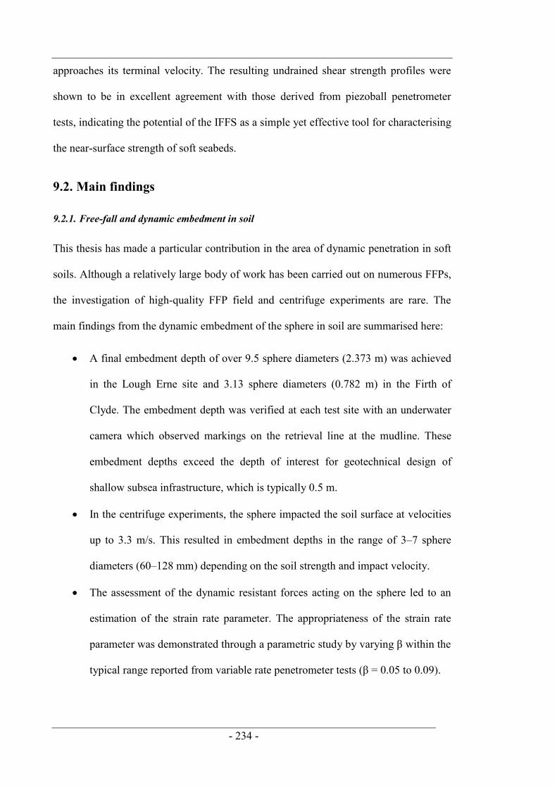
- 234 -
approaches its terminal velocity. The resulting undrained shear strength profiles were
shown to be in excellent agreement with those derived from piezoball penetrometer
tests, indicating the potential of the IFFS as a simple yet effective tool for characterising
the near-surface strength of soft seabeds.
9.2. Main findings
9.2.1. Free-fall and dynamic embedment in soil
This thesis has made a particular contribution in the area of dynamic penetration in soft
soils. Although a relatively large body of work has been carried out on numerous FFPs,
the investigation of high-quality FFP field and centrifuge experiments are rare. The
main findings from the dynamic embedment of the sphere in soil are summarised here:
A final embedment depth of over 9.5 sphere diameters (2.373 m) was achieved
in the Lough Erne site and 3.13 sphere diameters (0.782 m) in the Firth of
Clyde. The embedment depth was verified at each test site with an underwater
camera which observed markings on the retrieval line at the mudline. These
embedment depths exceed the depth of interest for geotechnical design of
shallow subsea infrastructure, which is typically 0.5 m.
In the centrifuge experiments, the sphere impacted the soil surface at velocities
up to 3.3 m/s. This resulted in embedment depths in the range of 3–7 sphere
diameters (60–128 mm) depending on the soil strength and impact velocity.
The assessment of the dynamic resistant forces acting on the sphere led to an
estimation of the strain rate parameter. The appropriateness of the strain rate
parameter was demonstrated through a parametric study by varying β within the
typical range reported from variable rate penetrometer tests (β = 0.05 to 0.09).
- 235 -
Higher strain rates were achieved in the centrifuge tests, with a maximum v/D =
130 s-1 compared to a maximum v/D = 31 s-1 in the field. In both sets of
experiments, a best-fit strain rate parameter of β = 0.07 was calculated.
Analysis of the motion data recorded by the IMU during dynamic embedment
in soil led to the development of a new theoretical framework that describes the
forces acting on a IFFS during dynamic embedment in soil. The framework is
cast in terms of both fluid mechanics drag resistance and geotechnical shear
resistance, but formulated in terms of a single capacity factor. It was found that
for low non-Newtonian Reynolds Numbers, Renon-Newtonian, the capacity factor
approaches the conventional bearing capacity factor, but may be up to two
orders of magnitude higher at high Renon-Newtonian.
The theoretical framework was used to calculate the undrained shear strength in
5 soils, 2 field soils (Chapter 7) and 3 soils in the centrifuge (Chapter 8). The
calculated su profiles in each soil compared very well to the undrained shear
strength profile measured in push-in ball or piezoball penetrometer tests,
verifying the merit of the IFFS as a time-effective and reliable site investigation
tool for soft soils.
9.2.2. MEMS accelerometers in the centrifuge
The thesis has made an original contribution to the area of geotechnical centrifuge
testing using MEMS accelerometers. The thesis described in detail two measurement
systems based on a single-axis and triple-axis accelerometer. To the authors knowledge
these are first reported experiments using MEMS accelerometers to measure the
dynamic forces on a FFP in a geotechnical centrifuge. The initial experiments involved
a comparison between a MEMS and piezoelectric single-axis accelerometer measuring
the motion response of a dynamically installed anchor as it free-falls through air and
- 236 -
embeds within a centrifuge soil sample (described in Chapter 6). The main findings
from the direct comparison between the two accelerometers are summarised here:
It was found that the performance of the MEMS accelerometer was superior to
the piezoelectric accelerometer during the free-fall phase and similar in
performance during the embedment phase in soil.
An assessment of the anchor tilt angle was explored in Chapter 6 and it was
shown that tilt angles up to 10˚ have negligible effect on the velocity profile,
with a maximum reduction in impact velocity and final embedment depth of
1.4% and 1% respectively. For a tilt angle of 20˚, the impact velocity reduces
by 5.4% and the final embedment depth 3.7% and for a tilt angle of 30˚, the
impact velocity reduces by 11.8% and final embedment depth reduces by 8.1%.
The second major contribution using a MEMS accelerometer was described in Chapter
8 where the vertical penetrating resistance on a model IFFS in the centrifuge was
measured using a triple-axis accelerometer. The tri-axis accelerometer was required
because the sphere can undergo excessive tilt whilst in free-fall in water and embedment
in soil. The method used the resultant acceleration computed from the three component
accelerations to calculate the vertical penetration resistance. The method was shown to
be able to accurately capture the forces acting on the sphere during penetration in soil.
9.2.3. Shallow penetration framework
The shallow penetration effects of a ball penetrometer were assessed through a suite of
centrifuge tests (described in Chapter 4) and a series of equations have been proposed
that offer a more rigorous and reliable means of assessing soil strength in the upper few
metres of the seabed. The tests were carried out with an 11.3 mm diameter ball
penetrometer penetrating kaolin clay under undrained conditions over a range of

- 237 -
normalised strength ratios, su/γ'D = 0.07 to 2.7. The tests aimed to capture the influence
of two mechanisms that are often overlooked: (i) the varying soil buoyancy with
penetration depth and (ii) the reduced bearing factor, Nc-shallow, arising from the shallow
failure mechanism. It was shown that the shallow failure mechanism can significantly
influence the estimation of su and can extend several diameters from the mudline. For
example, using a 0.25 m diameter IFFS, the correction can extend to a depth of up to ~1
m and for a push-in ball penetrometer test using a 113 mm diameter ball, the shallow
correction may extend to a depth of up to ~0.5 m. The framework comprises a series of
simple formulae that are discussed briefly here:
A correlation for the transition depth of a ball penetrometer, which is the depth
at which soil flows over the top of the ball, has been derived. The transition
depth indicates the depth where the soil flow mechanism changes from a
shallow heave-dominated flow to a deep flow round failure mechanism. The
original centrifuge data (Chapter 4) were combined with reinterpreted data from
LDFE analyses to form a unique relationship between the transition depth and
the normalised strength ratio over the range su/γ'D ≈ 0.07 to 40.
A correlation for the shallow bearing capacity factor has been derived; this
formulation accounts for the varying bearing capacity factor from a low number
at the soil surface that gradually increases to the limiting bearing capacity
factor, Nc-deep at the transition depth. The bearing factor component of the
correction is particularly important in stiff soils, due to the deeper penetration
required to mobilise the deep flow round failure mechanism.
A novel analytical closed-form solution for the varying soil buoyancy force
with depth has been proposed (Appendix 1). The formulation assesses the soil
buoyancy in the case where an open conical hole develops due to the passage of

- 238 -
the sphere. This is an important consideration in very soft soil with zero
mudline strength where the buoyancy resistance increases to almost 70% of the
geotechnical resistance during shallow penetration, and is independent of the
penetrometer diameter at all penetration depths.

- 239 -
REFERENCES
Abelev, A., Tubbs, K. & Valent, P., 2009b. Numerical investigation of dynamic free-
fall penetrometers in soft cohesive marine sediments using a finite difference
approach. Proceedings of OCEANS 2009: Marine Technology for Our Future:
Global and Local Challenges, MTS/IEEE Biloxi, Biloxi, MS, pp. 1–10.
Abelev, A. & Valent, P., 2009. Strain-rate dependency of strength and viscosity of soft
marine deposits of the Gulf of Mexico. Proceedings of OCEANS 2009: Marine
Technology for Our Future: Global and Local Challenges, MTS/IEEE Biloxi,
Biloxi, MS, pp. 1–9.
Achenbach, E., 1971. Influence of surface roughness on the cross-flow around a circular
cylinder. Journal of Fluid Mechanics, 46 pp. 321–335
Achenbach, E., 1972. Experiments on the flow past spheres at very high Reynolds
numbers. Journal of Fluid Mechanics. 54, pp. 565–575.
Akal, T. & Stoll, R. D., 1995. An expendable penetrometer for rapid assessment of
seafloor parameters. Proceedings of OCEANS 1995: Challenges of Our
Changing Global Environment, MTS/IEEE, San Diego, CA, pp. 1822–1826.
Allen, H. S., 1900. The motion of a sphere in a viscous fluid. Philosophical Magazine,
50, pp. 519–534.
Allmond, J. D., Hakhamaneshi, M., Wilson, D. W., & Kutter, B. L., 2014, Advances in
measuring rotation with MEMS accelerometers. Proceedings of the Eight
- 240 -
International Conference on Physical Modelling in Geotechnics, Perth,
Australia, 14–17 January 2014. 1, pp. 353–359.
Andersen, K. H., Murff, J. D., Randolph, M. F., Cluckey, E. C., Erbrich, C. T., Jostad,
H. P., Hansen, B., Aubeny, C., Sharma, P. & Supachawarote, C., 2005. Suction
anchors for deepwater applications. Proceedings of the 1st International
Symposium on Frontiers in Geotechnics, Perth, Australia, pp. 3–30.
Aubeny, C. P. & Shi, H., 2006. Interpretation of impact penetration measurements in
soft clays. Journal of Geotechnical and Geoenvironmental Engineering, ASCE,
132(6), pp. 770–777.
Audibert, J. M. E., Movant, M. N., Won, J. Y, & Gilbert, R. B., 2006. Toprepdo piles:
laboratory and field research. Proceedings of the 16th International Offshore
and Polar Engineering Conference, San Francisco, California, USA, pp. 135–
142.
Bacon, D. L. & Reid, E. G., 1924. The resistance of spheres in wind tunnels and in air.
Nut. Adv. Corn. Aero. Report. No. 185.
Bakić, V., 2004. Experimental investigation of a flow around a sphere. Thermal
Science, 8(1), pp. 63–81.
Balderas Meca, J., 2004. Rate effects of rapid loading in clay soils. PhD thesis, The
University of Sheffield.
Baligh, M.M., Azzouz, A.S., Wissa, A.Z.E., Martin, R.T. & Morrison, M.H., 1981. The
piezocone penetrometer: cone penetration testing and experience. Proc. ASCE
Conference on Cone Penetration Testing, St Louis, pp. 247–263.

- 241 -
Beard, K. V. & Pruppacher, H. R., 1969. A determination of the terminal velocity and
drag of small water drops by means of a wind tunnel. Journal of Atmospheric
Sciences, 26, pp. 1066–1072.
Beard, R. M., 1977. Expendable doppler penetrometer: a performance evaluation,
Technical Report R855, Civil Engineering Laboratory, Port Hueneme,
California.
Beard, R. M., 1981. A penetrometer for deep ocean seafloor exploration. Proceedings of
OCEANS 1981: The ocean an international workplace, MTS/IEEE, Boston, MA,
United States, pp. 668–673.
Beard, R. M., 1985. Expendable doppler penetrometer for deep ocean sediment
measurements. ASTM Special Technical Publication, 883, pp. 101–124.
Bennett V., Abdoun T., Shantz T., Jang D., & Thevanayagam, S., 2009, Design and
characterization of a compact array of MEMS accelerometers for geotechnical
instrumentation, Smart Structures and Systems, 5(6), pp. 663–679.
Bhattacharya, S., Murali, K., Lombardi, D., Crewe, A. & Alexander, N., 2012.
Economic MEMS based 3-axis water proof accelerometer for dynamic geo-
engineering applications. Soil Dynamics and Earthquake Engineering, 36, pp.
111–118.
Bienen, B. Ragni, F., Cassidy. M. J. & Stanier, S. A., 2015. Effects of consolidation
under a penetrating footing in carbonate silty clay. Journal of Geotechnical and
Geoenvironmental Engineering, 04015040.
Bienen, B., Cassidy. M. J., Randolph, M. F. & Tel. K. L., 2015. Characterisation of
undrained shear strength using statistical methods. 2nd International Symposium
on Frontiers in Offshore Geotechnics, Perth, Australia, pp. 661–666.
- 242 -
Biscontin, G. & Pestana, J. M., 2001. Influence of peripheral velocity on vane shear
strength of an artificial clay. Geotechnical Testing Journal, ASTM, 24(4), pp.
423–429.
Bjerrum, L., 1973. Problems of soil mechanics and construction on soft clays and
structurally unstable soils (collapsible, expansive and others). Proceedings of the
Eighth International Conference on Soil Mechanics and Foundation
Engineering, Moscow, pp. 111–159.
Blake, A. P., O‟Loughlin, C.D., Morton, J. P., O‟Beirne, C., Gaudin, C. & White, D. J.,
2015. In-situ measurement of the dynamic penetration of free-fall projectiles in
soft soils using a low cost inertial measurement unit. Geotechnical Testing
Journal, ASTM. DOI: 10.1520/GTJ20140135.
Blake, A. P. & O‟Loughlin, C. D., 2012. Field testing of a reduced scale dynamically
embedded plate anchor. Proceedings of the 7th International Conference in
Offshore Site Investigation and Geotechnics, London, United Kingdom, pp.
621–628.
Blake, A. P. & O‟Loughlin, C. D., 2015. Installation of dynamically embedded plate
anchors as assessed through field tests. Canadian Geotechnical Journal. 0, 0,
10.1139/cgj-2014-0327
Boukpeti, N., White, D. J., Randolph, M. F. & Low, H. E., 2012. Strength of fine-
grained soils at the solid-fluid transition. Géotechnique, 62(3), pp. 213–226.
Bowman, L., March, R., Orenberg, P., True, D. & Herrmann, H., 1995. Evaluation of
dropped versus static cone penetrometers at a calcareous cohesive site.
Proceedings of OCEANS 1995: Challenges of Our Changing Global
Environment, MTS/IEEE, San Diego, CA, pp. 1846–1858.
- 243 -
Boylan, N., Long, M., Ward, D., Barwise, A. & Georgious, B., 2007. Full flow
penetrometer testing in Bothkennar clay. Proceedings of the 6th International
Conference, Society for Underwater Technology, Offshore Site Investigation and
Geotechnics (SUT-OSIG), London, pp. 177–186.
Brandão, F. E. N., Henriques, C. C. D., Araújo, J. B., Ferreira, O. C. G. & Amaral, C.
D. S., 2006. Albacora Leste field development - FPSO P-50 mooring system
concept and installation. Proceedings of the Offshore Technology Conference,
Houston, Texas, USA, OTC 18243.
Briaud, J. L., Garland, E. & Felio, G. Y., 1984. Rate of loading parameters for vertically
loaded piles in clay. In Proceedings of the 16th Annual Offshore Technology
Conference, Houston, Texas, USA, paper OTC 4694, pp. 407–412.
Britto, A. M. & Kusakabe, O., 1982. Stability of unsupported axisymmetric excavations
in soft clay. Géotechnique 32(3), pp. 261–270.
Britto, A. M. & Kusakabe, O., 1983. Stability of axisymmetric excavations in clays.
Journal of Geotechnical and Geoenvironmental Engineering, ASCE, 109(5), pp.
666–681.
Brown, M. J. & Hyde, A. F. L., 2008b. Rate effects from pile shaft resistance
measurements. Canadian Geotechnical Journal, 45(3), pp. 425–431.
Brown, P. P. & Lawler, D. F., 2003. Sphere drag and settling velocity revisited. Journal
of Environmental Engineering, 129, pp. 222–231.
Carter, J. P., Nazem, M. & Airey, D. W., 2013. Analysis of Dynamic Loading and
Penetration of Soils - Application to site investigation and ground improvement.
International Conference on Geotechnical Engineering, ICGE 12, Hammamet,
Tunisia.
- 244 -
Casagrande, A. & Wilson, S., 1951. Effect of rate of loading on the strength of clays
and shales at constant water content. Géotechnique, 2(3), pp. 251–563.
Cenac Π, W. A., 2011. Vertically loaded anchor: drag coefficient, fall velocity and
penetration depth using laboratory measurements. Master‟s thesis, Texas A&M
University, College Station, USA.
Chari, T. R., Smith, W. G. & Zielinski, A., 1978. Use of free fall penetrometer in sea
floor engineering. Proceedings of OCEANS 1978: The Ocean Challenge,
MTS/IEEE, Washington, D.C., pp. 686–691.
Chatterjee, S., Randolph, M. F. & White, D. J., 2012. The effects of penetration rate and
strain softening on the vertical penetration resistance of seabed pipelines.
Géotechnique 62(7), pp. 573–582.
Chow, S. H. & Airey, D. H., 2010. Laboratory free falling penetrometer test into clay.
Proceeding of the 2nd International Symposium on Frontiers in Offshore
Geotechnics, Perth, Australia, pp. 265–270.
Chow, S. H., 2013. Free-falling penetrometer tests in clay. PhD thesis, The University
of Sydney, Sydney, Australia.
Chow, S. H., O‟Loughlin, C. D. & Randolph, M. F. (2014). Soil strength estimation and
pore pressure dissipation for free-fall piezocones in soft clay. Géotechnique,
64(10), PP. 817–827.
Chung, S. F. & Randolph, M. F., 2004. Penetration resistance in soft clay for different
shaped penetrometers. In A. V. da Fonseca & P. W. Mayne, eds. Proc., ISC-2 on
Geotechnical and Geophysical Site Characterization. Portugal: Millpress,
Rotterdam, pp. 671–677.
- 245 -
Chung, S. F., Randolph, M. F. & Schneider, J. A., 2006. Effect of penetration rate on
penetrometer resistance in clay. Journal of Geotechnical and Geoenvironmental
Engineering, ASCE, 132(9), pp. 1188–1196.
Cilingir, U. C. & Madabhushi, G., 2011. A model study on the effects of input motion
on the seismic behavior of tunnels. Soil Dynamics and Earthquake Engineering,
31, pp. 452–462.
Cocjin, M. J., Gourvenec, S. M., White, D. J. & Randolph, M. F., 2014. Tolerably
mobile subsea foundations – observations of performance. Géotechnique,
64(10), pp. 817–827.
Colp, J., Caudle, W. & Schuster, C., 1975. Penetrometer system for measuring in situ
properties of marine sediment. Proceedings of OCEANS 1975, MTS/IEEE, San
Diego, CA, pp. 405–411.
Colreavy, C., O‟Loughlin, C. D. & Ward, D., 2012. Piezoball tests in a soft lake
sediments. Proceedings of the 4th International Conference on Geotechnical
and Geophysical Site Characterisation, Porto de Galinhas, Brazil, pp. 597–602.
Coussot, P., Laigle. D., Arratano, M., Deganutti, A. & Marchi, L., 1998. Direct
determination of rheological characteristics of debris flow. J. Hydraul. Eng. 124,
pp. 865–868.
CYR, R., Ardus, D. A. & Champ, M. A., 1990. Sea bed sampling with an expendable
acoustic penetrometer system. In D. A. Ardus & M. A. Champ (eds), Ocean
Resources, 2, Kluwer Academic: Netherlands, pp. 45–56.
Davies, C. N., 1945. Definitive equations for the fluid resistance of spheres.
Proceedings of the Physical Society, London, 57, pp. 259–270.
- 246 -
Dayal, U. & Allen, J. H., 1973. Instrumented cone penetrometer. Canadian
Geotechnical Journal, 10, pp. 397–409.
Dayal, U., 1974. Instrumented impact cone penetrometer. PhD thesis, Memorial
University of Newfoundland.
Dayal, U., Allen, J. & Jones, J., 1975. Use of an impact penetrometer for the evaluation
of the in-situ strength of marine sediments. Marine Georesources &
Geotechnology, 1(2), pp. 73–89.
Deep Sea Anchors., 2011. DPA™ fabricated at Western Ship Yard in Klaipeda,
Lithuania [image online] available: http://www.deepseaanchors.com/News.html
[accessed 4 November 2011].
DeJong, J. T., Yafrate, N. J., DeGroot, D. J. & Jakubowski, J., 2004. Evaluation of the
undrained shear strength profile in soft layered clay using full-flow probes.
Proceedings of the 2nd Inernational Confewrence on Site Characterisation,
Porto. Rotterdam, pp. 679–686.
DeJong, J., Yafrate, N., DeGroot, D., Low, H. E. & Randolph, M. F., 2010.
Recommended practice for full-flow penetrometer testing and analysis,
Geotechnical Testing Journal, ASTM, 33(2), pp. 137–149.
Deglo de Besses, B. D., Magnin, A. & Jay, P., 2003.Viscoplastic flow around a cylinder
in an infinite medium. Journal of Non-Newtonian Fluid Mechanics, 115, pp. 27–
49.
Denness, B., Berry, A., Darwell, J. & Nakamura, T., 1981. Dynamic seabed penetration.
Proceedings of OCEANS 1981: The ocean; an international workplace,
MTS/IEEE, Boston, MA, United States, pp. 662–667.

- 247 -
Dennis, S. C. R. & Walker, J. D. A., 1971. Calculation of the steady flow past a sphere
at low and moderate Reynolds numbers. Journal of Fluid Mechanics., 48, pp.
771–789.
Díaz-Rodríguez, J. A., Lozano-Santa Cruz, R., Davila-Alcocer, V. M., Vallejo, E. &
Girón, P., 1998. Physical, chemical, and mineralogical properties of Mexico
City sediments: A geotechnical perspective. Canadian Geotechnical Journal,
35(4), pp. 600–610.
Diaz-Rodriguez, J. A. & Martinez-Vasquez, J. J., 2005. Strain rate behaviour of Mexico
City Soils. Proceedings of the 16th International Conference on Soil Mechanics
and Geotechnical Engineering, Osaka, Japan, 2, pp. 333–336.
Douglas, B. L. & Wapner, M. P., 1996. Test results of the doppler penetrometer
seafloor sediment profiling system. Proceedings of OCEANS 1996: Prospects
for the 21st Century, MTS/IEEE, Fort Lauderdale, Florida, United States, 2, pp.
722–727.
Einav, I., Klar, A., O'Loughlin, C. D. & Randolph, M. F., 2004. Numerical modelling of
Deep Penetrating Anchors. Proceedings of the 9th Australian and New Zealand
Conference on Geomechanics, Auckland, New Zealand, Vol 2, pp. 818–824.
Einav, I. & Randolph, M. F., 2005. Combining upper bound and strain path methods for
evaluating penetration resistance. International Journal for Numerical Methods
in Engineering, 63(14), pp. 1991–2016.
Einav, I. & Randolph, M. F., 2006. Effect of strain rate on mobilised strength and
thickness of curved shear bands. Géotechnique, 56(7), pp. 501–504.

- 248 -
Elsworth, D. & Lee, D. S., 2005. Indentation of a free-falling lance penetrometer into a
poroelastic seabed. International Journal for Numerical and Analytical Methods
in Geomechanics, 29(2), pp. 141–162.
Fage, A. 1936 Experiments on a sphere at critical Reynolds numbers. Brit. Aero. Res.
Counc. Rep.& Mem. pp.1766.
Feng, X., Randolph, M.F., Gourvenec, S. & Wallerand R., 2013. Design approach for
rectangular mudmats under fully three-dimensional loading. Géotechnique,
64(1), pp. 51–63.
Fernandes, A. C., Araujo, J. B., Lima de Almeida, J. C., Machado, R. D. & Matos, V.,
2006. Torpedo anchor installation hydrodynamics. Journal of Offshore
Mechanics and Artic Engineering, 128(11), pp. 286–293.
Finnie, I. M. S. & Randolph, M. F., 1994. Punch-through and liquefaction induced
failure of shallow foundations on calcareous sediments. Proceedings of the
International Conference on behaviour of offshore structures, Boston, pp. 217–
230.
Finnemore, E. & Franzini, J., 2001. Fluid Mechanics With Engineering Applications –
McGraw-Hill Education.
Fossen, T. I., 2011, Handbook of marine craft hydrodynamics and motion control, John
Wiley & Sons, Ltd., Chichester, United Kingdom.
Freeman, T.J. & Burdett, J. R. F., 1986. Deep ocean model penetrator experiments.
Commission of the European Communities Nuclear Science and Technology
Report EUR 10502, Commission of the European Communities, Brussels,
Luxembourg.
- 249 -
Freeman, T. J., Murray, C. N., Francis, T. J. G., McPhail, S. D. & Schultheiss, P. J.,
1984. Modelling radioactive waste disposal by penetrator experiments in the
abyssal Atlantic Ocean. Nature, 310, pp. 130–133.
Freeman, T. J., Murray, C. N. & Schuttenhelm, R. T. E., 1988. The Tyro 86 penetrator
experiments at Great Meteor East. In Oceanology’88: Proceedings of an
international conference. London: Graham & Trotman, pp. 217–226.
Freeman, T. J. & Schuttenhelm, R. T. E., 1990. A geotechnical investigation of a deep
ocean site. Geotechnical Engineering of Ocean Waste Disposal, ASTM STP
1087, pp. 255–275.
Furlong, A., Osler, J., Christian, H., Cunningham, D & Pecknold, S., 2006. The Moving
Vessel Profiler (MVP) - a rapid environmental assessment tool for the collection
of water column profiles and sediment classification. Proceedings of Undersea
Defence Technology Pacific Conference 2006, San Diego, US, pp. 1–13.
Gaudin, C., O‟Loughlin, C. D., Hossain, M. S & Zimmerman, E. H., 2013. The
performance of dynamically embedded anchors in calcareous silt. Proceeding of
the 32nd International Conference on Offshore Mechanics and Arctic
Engineering, Nantes, France, Vol. 6, OMAE2013-10115.
Gaudin, C., White, D. J., Boylan, N., Breen, J., Brown, T., De Catania, S. & Hortin, P.,
2009. A wireless high-speed data acquisition system for geotechnical centrifuge
model testing. Measurement Science and Technology, 20(9): 095709,
http://dx.doi.org/10.1088/0957-0233/20/9/095709.
Georgiadis, M., 1991. Landslide drag forces on pipelines, Soils and Foundations.
Japanese Society of Soil mechanics and Foundation Engineering. 31(1), pp.
156–161.
- 250 -
Gibson, G. C. & Coyle, H. M., 1968. Soil damping constants related to common soil
properties in sands and clays, Technical Report 125-1,Texas Transportation
Institute.
Gibson, C. E., 1998. Lough Erne. In: Moriarty, C. (Ed.), Studies of Irish Lakes and
Rivers. Marine Institute, Dublin, pp. 64–72.
Gilbert, R. B., Morvant, M. & Audibert, J., 2008. Torpedo piles joint industry project –
model torpedo pile tests in kaolinite test beds, Report No. 02/08B187, Offshore
Technology Research Center, Texas A & M University.
Goin, K. L. & Lawrence, W. R., 1968. Subsonic drag of spheres at Reynolds numbers
from 200 to 10,000. AIAA J., 6, pp. 961–962.
Govardhan, R. & Williamson, C. H. K. 2005 Votex-induced vibration of a sphere.
Journal of Fluid Mechanics. 531, pp. 11–47.
Graham, J., Crooks, J. H .A. & Bell, A. L., 1983. Time effects on the stress-strain
behaviour of natural soft clays. Géotechnique, 33(3), pp. 327–340.
Gunn, R. & Kinzer, G. D., 1949. The terminal velocity of fall for water droplets in
stagnant air. J. Meteorol., 6, pp. 243–250.
Hasanloo, D., Pang, H. & Yu, G., 2012. On the estimation of the falling velocity and
drag coefficient of torpedo anchor during acceleration. Ocean Engineering, 42,
pp. 135–146.
Hartman, M., Trnka, O. , & Svoboda, K.,1994. Free settling of nonspherical particles.
Industrial & Engineering Chemistry Research,. 33, pp. 1979–1983.
Hossain, M. S, Kim, Y. & Wang, D., 2013. Physical and numerical modelling of
installation and pull-out of dynamically penetrating anchors in clay and silt.
- 251 -
Proceeding of the 32nd International Conference on Offshore Mechanics and
Arctic Engineering, Nantes, France, Vol. 6, OMAE2013-10322.
Hossain M. S., Hu Y., Randolph M. F. & White D. J., 2005. Limiting cavity depth for
spudcan foundations penetrating clay. Géotechnique, 55(9), pp. 679–690.
Hossain, M. S., Kim, Y. & Gaudin, C., 2014. Experimental investigation of installation
and pullout of dynamically penetrating anchors in clay and silt. Journal of
Geotechnical and Geoenvironmental Engineering, 140(7), pp. 04014026.
Houlsby, G.T. & Wroth, C.P., 1983. Calculation of stresses on shallow penetrometers
and footings. Proceedings of IUTAM/IUGG Symposium on Sebed Mechanics.
Newcastle upon Tyne, pp. 107–112.
House, A. R., Oliveira, J. R. M. S. & Randolph, M. F., 2001. Evaluating the coefficient
of consolidation using penetration tests. International Journal of Physical
Modelling in Geotechnics, 1(3), pp. 17–25.
Houwink, R., 1952. Elasticity, plasticity and structure of matter. Cambridge University
Press.
Hu, P., Stainer, S. A., Cassidy, M. J. & Wang, D., 2014. Predicting peak resistance of
spudcan penetrating sand overlying clay. Journal of Geotechnical and
Geoenvironmental Engineering ASCE, 140(2).
Hurst, R. B. & Murdoch, S., 1991. Measurement of sediment shear strength for mine
impact burial predictions. Report of the 18th Meeting of the Mines and Mine
Countermeasures Technology Panel GTP-13.
Hyde, A. E. L., Anderson, W. F. & Robinson, S. A., 2000. Rate effects in clay soils and
their relevance to statnamic pile testing. In Statnamic Loading Test: Proceedings
of the 2nd International Statnamic Seminar, Tokyo, Japan, pp. 303–309.
- 252 -
Jeanjean, P., Spikula, D. & Young, A., (2012). Technical vetting of free-fall cone
penetrometer. Proceedings of 7th international offshore site investigation and
geotechnics conference: Integrated geotechnologies – present and future, pp.
15–18. London UK: Society for Underwater Technology.
Jeong, S. W., Leroueil, S. & Locat, J., 2009. Applicability of power law for describing
the rheology of soils of different origins and characteristics. Canadian
Geotechnical Journal, 46, pp. 1011–1023.
Jones, D. A. & Clarke, D. B., 2008. Simulation of flow past a sphere using the
FLUENT code. Defence Science and Technology Organisation for the
Australian Government Department of Defence. DSTO-TR-2232.
Jonkman, J. M., 2007, Dynamics modelling and loads analysis of an offshore floating
wind turbine. National Renewable Energy Laboratory Technical Report
NREL/TP-500-41958, National Renewable Energy Laboratory, Golden,
Colorado, United States.
Kee, R. & Ims, B. W., 1984. Geotechnical hazards associated with leg penetration of
jack-up rigs. Seabed Mechanics, pp. 169–174. London: Graham & Trotman.
Kelleher, P. & Randolph, M. F., 2005. Seabed geotechnical characterisation with a ball
penetrometer deployed from the portable remotely operated drill. Proceedings of
International Symposium on Frontiers in Offshore Geotechnics (ISFOG), pp.
365–371.
King, K., Yoon, S. W., Perkins, N. C., & Najafi, K., 2008, Wireless MEMS inertial
sensor system for golf swing dynamics, Sensors and Actuators, 141(2), pp. 619–
630.
- 253 -
Kunitaki, D. M. K. N., De Lima, B. S. L. P., Evsukoff, A. G. & Jacob, B. P., 2008.
Probabilistic and fuzzy arithmetic approaches for the treatment of uncertainties
in the installation of torpedo piles, Mathematical Problems in Engineering,
Article ID 512343.
Kusakabe, O., Suzuki, H. & Nakase, A., 1986. An upper bound calculation on bearing
capacity of a circular footing on a non-homogeneous clay. Soils and
foundations, 26(3), pp.143–148.
Ladd, C. C., Foot, R., Ishihara, K., Schlosser, F. & Poulos, H. G., 1977. Stress–
deformation and strength characteristics. Proceedings of the 9th International
Conference on Soil Mechanics. Found. Engng, Tokyo 2, pp. 421–494.
Lamb, H., 1932. Hydrodynamics. Cambridge University Press.
Lavieri, R. S., Tannuri, E. A., Fujarra, A. L. C, & Corr a, D. C., 2011. Aided Inertial
Measurement System Applied to Torpedo Pile Trajectory Reconstruction. 30th
International Conference on Ocean, Offshore and Arctic Engineering,
Rotterdam, The Netherlands, 1, pp. 59–66.
Lafferty, B., Quinn, R. & Breen, C., 2006. A side-scan sonar and high-resolution chirp
sub-bottom profile study of the natural and anthropogenic sedimentary record of
Lower Lough Erne, northwestern Ireland. Journal of Archaeological Science, 33
pp. 756–766.
Lefebvre, G. & LeBoeuf, D., 1987. Rate effects and cyclic loading of sensitive clays.
Journal of Geotechnical Engineering, 113(5), pp. 476–489.
Lehane, B. M., O‟Loughlin, C. D., Gaudin, C. & Randolph, M. F., 2009. Rate effects on
penetrometer resistance in kaolin. Géotechnique, 59(1), pp. 41–52.

- 254 -
Levacher, D., 1985. Penetrometre a chute libre: impact et penetration dans des argiles
reconstituees. Canadian Geotechnical Journal, 22(1), pp. 129–135.
Levy, F. M., & Richards, D. J., 2012, Rapid soil displacements from MEMS
accelerometers, Proceedings of the 30th IMAC Conference on Structural
Dynamics, Jacksonville, Florida, United States, 30 January–2 February 2012. 1,
pp. 197–208.
Liebster, H. 1927. Uber den widerstand von kugeln. Annalen der Physik (Leipzig), 82,
541 562.
Lieng, J. T., Hove, F. & Tjelta, T. I., 1999. Deep Penetrating Anchor : subseabed
deepwater anchor concept for floaters and other installations. Proceedings of the
9th International Offshore & Polar Engineering Conference, Brest, France, pp.
613–619.
Lieng, J. T., Tjelta, T . I. & Skaugset, K., 2010. Installation of two prototype deep
penetrating anchors at the Gjøa field in the North Sea. Proceedings of the
Offshore Technology Conference, Houston, USA, OTC 20758.
Liu, X. D., Sun, J., Yi, J. T., Lee, F. H., Gu, H. & Chow, Y. K., 2014. Physical and
Numerical Modeling of the Performance of Dynamically Installed Anchors in
Clay. 33rd International Conference on Ocean, Offshore and Arctic Engineering
Volume 1A: Offshore Technology San Francisco, California, USA.
Long, M. & Gudjonsson, G.T., 2004. T-bar testing in Irish soils. Proceedings of the 2nd
International Conference on Site Characterisation, Porto, pp. 719–726.
Low, H. E., Randolph M. F. & Kelleher, P., 2007. Comparison of pore pressure
generation and dissipation rates from cone and ball penetrometers. Proceedings
of the 6th International Conference of the Society for Underwater Technology,

- 255 -
Offshore Site Investigation and Geotechnics (SUT-OSIG), London, pp. 547–
556.
Low, H. E., Randolph, M. F., DeJong, J. T. & Yafrate, N. J., 2008. Variable rate full-
flow penetration tests in intact and remoulded soil. Proceedings of the 3rd
International Conference on Site Characterization, Taipei, pp. 1087–1092.
Low, H.E., Randolph, M. F., Lunne, T., Andersen, K. H. & Sjursen, M.A. 2011. Effect
of soil characteristics on relative values of piezocone, T-bar and ball penetration
resistances. Géotechnique, 61(8), pp. 651–664.
Lu, Q., Hu, Y. & Randolph, M. F., 2000. FE analysis for T-bar and spherical
penetrometers in cohesive soil. Proceedings of the 10th International Offshore
and Polar Engng Conference. Seattle, 2, pp. 617–623.
Lu, Q., Hu, Y. & Randolph, M. F., 2001. Deep penetration in soft clay with strength
increasing with depth. Proceedings of the 11th International Offshore and Polar
Engng Conference. Stavanger 2, pp. 453–458.
Lunne, T., Christoffersen, H. P. and Tjelta, T. I., 1985. Engineering use of piezocone
data in North Sea clays. Proceedings of the 11th International Conference on
Soil Mechanics and Foundation Engineering, San Francisco, 2, pp. 907–912.
Lunne, T., Robertson, P. K. and Powell, J. J. M., 1997. Cone Penetration Testing in
Geotechnical Engineering, Blackie Academic and Professional, London.
Lunne, T. 2001. In situ testing in offshore geotechnical investigations. Proceedings of
the International Conference on In Situ Measurement of Soil Properties and
Case Histories, Bali, pp. 61–81.
- 256 -
Lunne, T., Berre, T., Andersen, K. H. & Strandvik, S., 2006. Effects of sample
disturbance and consolidation procedures on measured shear strength of soft
marine Norwegian clays. Canadian Geotechnical Journal, 43(7), pp. 726–750.
Lunne, T. & Andersen, K. H., 2007. Soft clay shear strength parameters for deepwater
geotechnical design. Proceedings of the 6th International Offshore Site
Investigation and Geotechnics Conference: Confronting New Challenges and
Sharing Knowledge, London, UK, pp. 151–176.
Lunnon, R. G., 1928. Fluid resistance to moving spheres. Proceedings of the Royal
Society, London, 118, pp. 680–694.
Martin, C. M. & Randolph, M. F., 2001. Applications of the lower and upper bound
theorems of plasticity to collapse of circular foundations. Proceedings of the
International Conference on Computer Methods and Advances in
Geomechanics. Tuscon, pp. 1417–1428.
Martin, C. M. & Randolph, M. F., 2006. Upper-bound analysis of lateral pile capacity in
cohesive soil. Geotechnical Testing Journal, ASTM, 56(2), pp. 141–145.
Maxworthy, T., 1965. Accurate measurements of sphere drag at low reynolds numbers.
Journal of Fluid Mechanics., 23, pp. 369–372.
Maxworthy, T., 1969. Experiments on the flow around a sphere at high Reynolds
numbers. J. Appl. Mech., Trans. A.S.M.E. 36, pp. 598–607.
Medeiros., C. J., 2002. Low cost anchor system for flexible risers in deep waters.
Proceedings of Offshore Technology Conference. Houston, Texas, pp. 1–5.
Medeiros., C. J., Hassui, L. H. Machado, R. D., (1997). Pile for Anchoring Floating
Structures and Process for Installing the Same. United States Patent Number
6,106,199.0
- 257 -
Merifield R., White D. J. & Randolph M.F., 2009. The effect of surface heave on the
response of partially-embedded pipelines on clay. Journal of Geotechnical and
Geoenvironmental Engineering, ASCE, 135(6) pp. 819–829.
Mesri, G., Rokhsar, A. & Bohor, B. F., 1975. Composition and compressibility of
typical samples of Mexico City clay. Géotechnique, 24(3), pp. 527–554.
Meyerhof, G. G., 1972. Stability of slurry trench cuts in saturated clay. Proceedings of
the Speciality Conference on Performance of Earth and Earth Supported
Structures, 1, pp.1451–1466.
Migliore, H. J. & Lee, H. J., 1971. Seafloor penetration tests: presentation and analysis
of results. Naval Civil Engineering Laboratory Technical Note N-1178. Port
Hueneme, CA, pp. 60.
Millikan, C. B. & Klein, A. L., 1933. The effect of turbulence. An investigation of
maximum lift coefficient and turbulence in wind tunnels and in flight. Aircraft
Eng.
Mitchell, J. K. & Soga, K., 2005. Fundamentals of soil behavior. New York: Wiley.
Moller, W.,1938. Experimentelle untersuchungen zur hydrodynamik der kugel. Phys.
Z., 39, pp. 57–80.
Morrison, F. A., 2013. An Introduction to Fluid Mechanics. New York: Cambridge
University Press.
Morison, J. R., O'Brien, M. P., Johnson, J. W. & Schaaf, S. A., 1950. The force exerted
by surface waves on piles. Petroleum Transactions, 189, pp. 149–154.
Morton, J. P., & O‟Loughlin, C. D., 2012, Dynamic penetration of a sphere in clay,
Proceedings of the 7th International Conference in Offshore Site Investigation
- 258 -
and Geotechnics, London, United Kingdom, 12–14 September 2012. pp. 223–
230.
Morton, J. P., O‟Loughlin, C. D. & White, D. J. (2014). Strength assessment during
shallow penetration of a sphere in clay. Géotechnique Letters 4, October–
December, pp. 262–266.
Morton, J. P., O‟Loughlin, C. D. & White, D. J., 2015, An experimental assessment of
the dynamic resistance of a free-falling sphere in soft clay, in preparation.
Mulhearn, P. J., Poeckert, R. H. & Holtkamp, R. H., 1998. Report on penetrometer
comparisons from TTCP MAR-TP-13’s MCM Australian sea trials 1997
(MAST97) off Cairns, Great Barrier Reef, Australia, TTCP Report, DSTO,
Australia.
Mulhearn, P. J., Morgan, S., Poeckert, R. H. & Holtkamp, R. H., 1999. Penetrometer
comparison trials, Sydney Harbour, March 1998, TTCP Report, DSTO,
Australia.
Mulhearn, P. J., 2003. Influences of penetrometer tip geometry on bearing strength
estimates. International Journal of Offshore and Polar Engineering, 13(1), pp.
73–78.
Mulukutla, G. K., 2009. Determination of geotechnical properties of seafloor sediment.
PhD thesis, University of New Hampshire.
Murff, J. D. & Coyle, H. M. (1973). Low velocity penetration of kaolin clay. Journal of
Soil Mechanics & Foundations Div, 99(sm5).
Murff, J. D., Wagner, D. A. & Randolph, M. F., 2009. Pipe penetration in cohesive soil.
Géotechnique, 39(2), pp. 213–229.
- 259 -
Nakase, A. & Kamei, T., 1986. Influence of strain rate on undrained shear
characteristics of Ko-consolidated cohesive soils. Soils and Foundations, 26(1),
pp. 85–95.
Nazem, M. & Carter, J. P., 2010. Parametric study of a free-falling penetrometer in
clay-like soils. Proceedings of the International Symposium on Frontiers in
Geotechnics. ISFOG 2010, Perth, pp. 293–298.
Nazem, M., Carter, J. P., Airey, D. W. & Chow, S. H., 2012. Dynamic analysis of a
smooth penetrometer free falling into uniform clay. Géotechnique, 62(10), pp.
893–905.
Nebot, E. & Durrant-Whyte, H., 1999, Initial calibration and alignment of low cost
inertial navigation units for land vehicle applications, Journal of Robotics
Systems, 16(2), pp. 81–92.
Noureldin, A., Karamat, T. B., & Georgy, J., 2012, Fundamentals of inertial navigation,
satellite-based positioning and their integration, Springer-Verlag, Berlin,
Germany.
O‟Loughlin, C. D., Gaudin, C., Morton, J. P. & White D. J., 2014, MEMS
accelerometer for measuring dynamic penetration events in geotechnical
centrifuge tests, Physical Modelling in Geotechnics, Vol. 50, No. 5, pp. 31–39.
O‟Loughlin, C. D., Blake, A. P., Wang, D., Gaudin, C. & Randolph, M. F., 2013a. The
dynamically embedded plate anchor: results from an experimental and numerical
study. Proceedings of the 32nd International Conference in Ocean, Offshore
and Artic Engineering, Nantes, OMAE2013-11571.
- 260 -
O‟Loughlin, C. D., Richardson, M. D., Randolph, M. F. & Gaudin, C., 2013b.
Penetration of dynamically installed anchors in clay. Géotechnique, 63(11) pp.
909–919.
O‟Loughlin, C. D., Richardson, M. D. & Randolph, M. F., 2009. Centrifuge tests on
dynamically installed anchors. Proceedings of the ASME 28th International
Conference on Ocean, Offshore and Arctic Engineering, Honolulu, Hawaii, pp.
1–9.
O'Loughlin, C. D., Randolph, M. F. & Einav, I., 2004a. Physical modelling of deep
penetrating anchors. Proceedings of the 9th Australian and New Zealand
Conference on Geomechanics, Auckland, New Zealand, Vol. 2, pp. 710–716.
O'Loughlin, C. D., Randolph, M. F. & Richardson. M., 2004b. Experimental and
theoretical studies of deep penetrating anchors. Proceedings of the Offshore
Technology Conference, Houston, Texas, USA, 3–6 May 2004, OTC 16841.
Ortman, C. M., 2008. The effect of diameter on dynamic seabed penetration, Trident
Scholar Project Report No. 373, United States Naval Academy, Annapolis,
Maryland.
Øye, I., 2000. Simulation of trajectories for a deep penetrating anchor. CFD Norway
Report 250:2000, CFD Norway AS, Trondheim, Norway.
Pantaleone, J. & Messer, J., 2011. The added mass of a spherical projectile. American
Journal of Physics, 79(12), pp. 1202–1210.
Pazwash, H. & Robertson, J.M., 1969. Fluid-dynamic consideration of bottom
materials. Conference on Ocean Engeneering, ASCE - 1970.
Pazwash, H. & Robertson, J.M., 1975. Forces on bodies in Bingham fluids, Journal of
Hydraulic Research. 13, pp. 35–55.
- 261 -
Pettyjohn, E. S. & Christiansen, E. B., 1948. Effect of particle shape on free-settling
rates of isometric particles. Chem. Eng. Prog. 44, pp. 157–172.
Puech, A., Orozco-Caldero´n, M. & Foray, P., 2010. Mini T-bar testing at shallow
penetration. Proceedings of Frontiers in Offshore Geotechnics, Perth, pp. 305–
310.
Peuchen, J. & Mayne, P., 2007. Rate effects in vane shear testing. Proceedings of the
6th International Conference on Offshore Site Investigation and Geotechnics:
Confronting New Challenges and Sharing Knowledge. London, UK, pp. 187–
194.
Peuchen, J., Adrichem, J. & Hefer, P., 2005. Practice notes on push-in penetrometers
for offshore geotechnical investigation. pp. 19–21.
Poorooshasb, F. & James, R. G., 1989. Centrifuge modelling of heat-generating waste
disposal. Canadian Geotechnical Journal, 26, pp. 640–652.
Powell, J. & Quarterman, R., 1988. The interpretation of cone penetration tests in clays,
with particular reference to rate effects. In Penetration Testing 1988. Balkema,
Rotterdam, pp. 903–909.
Pruppacher, H. R. & Steinberger, E. H., 1968. Experimental determination of the drag
on a sphere at low Reynolds numbers. J. Appl. Phys. 39(9), pp. 4129–4132.
Quirós, G.W. & Young, A.G., 1988. Comparison of field vane, CPT and laboratory
strength data at Santa Barbara Channel site. Vane Shear Strength Testing of
Soils: Field and Laboratory Studies, ASTM STP 1014: pp. 306–317.
Raie, M. & Tassoulas, J. L., 2006. Numerical modeling of torpedo anchors. Final
project report – Phase I, Minerals Management Service, Project No. 557.
- 262 -
Raie, M. S. & Tassoulas, J. L., 2009. Installation of torpedo anchors: numerical
modelling. Journal of Geotechnical and Geoenvironmental Engineering,
135(12), pp. 1805–1813.
Randolph, M. F. & White, D. J., 2012. Interaction forces between pipelines and
submarine slides – a geotechnical viewpoint. Ocean Engineering, Vol. 48, pp.
32–37.
Randolph, M. F., Low, H. E. & Zhou, H., 2007, Keynote lecture: In situ testing for
design of pipeline and anchoring systems, Proceedings of the 6th International
Conference on Offshore Site Investigation and Geotechnics, London, United
Kingdom, 11–13 September 2007. pp. 251–262.
Randolph, M. F., 2004. Characterisation of soft sediments for offshore applications.
Proceedings of 2nd International Conference on Geotechnical and Geophysical
Site Characterization - ISC‟2, Porto. Rotterdam, pp. 209–232.
Randolph, M. F. & Hope, S., 2004. Effect of cone velocity on cone resistance and
excess pore pressures. Proceedings of the International Symposium on
Engineering Practice and Performance of Soft Deposits, Osaka, pp. 147–152.
Randolph, M. F., Martin, C. M. & Hu, Y., 2000. Limiting resistance of a spherical
penetrometer in cohesive material. Géotechnique, 50(5), pp. 573–582.
Randolph, M. F. & White, D. J., 2008. Pipeline embedment in deep water: processes
and quantitative assessment. Proceedings of Offshore Technology Conference,
Houston, 1, pp. 1–16.
Randolph, M. F., Hefer, P. A., Geise, J. M. & Watson, P. G., 1998. Improved seabed
strength profiling using T-bar penetrometer. Proceedings International

- 263 -
Conference on Offshore Site Investigation and Foundation Behavior - New
Frontiers, Society for Underwater Technology. London, UK, pp. 251–262.
Randolph, M. F. & Houlsby, G.T., 1984. The limiting pressure on a circular pile loaded
laterally in cohesive soil. Géotechnique, 34(4), pp. 613–623.
Ratcliffe, C., Heider, D. Crane, R., Krauthauser, K., Yoon, M.K. & Gillespie, J.W.,
2008. Investigation into the use of low cost MEMS accelerometers for vibration
based damage detection. Composite Structures, 82, pp.61–70.
Richardson, M. D., O‟Loughlin, C. D., Randolph, M. F. & Cunningham T. J., 2006.
Drum centrifuge modeling of dynamically penetrating anchors. Proceedings of
International Conference on Physical Modelling in Geotechnics, London. 1, pp.
673–678.
Richardson, M. D., 2008. Dynamically installed anchors for floating offshore
structures. PhD thesis, The University of Western Australia.
Richardson, M. D., O‟Loughlin, C. D., Randolph, M. F. & Gaudin, C., 2009. Setup
following installation of dynamic anchors in normally consolidated clay.
Journal of Geotechnical and Geoenvironmental Engineering ASCE, 135(4), pp.
487–496.
Rimon, Y. & Cheng, S. I., 1969. Numerical solution of a uniform flow over a sphere at
intermediate Reynolds numbers. Phys. Fluids, 12(5), pp. 949–959.
Pazwash, H., & Robertson, J. M., 1971. Fluid-Dynamic Consideration of Bottom
Materials. Journal of the Hydraulics Division, 97(9), pp. 1317-1329.
Roos, F. W. & Willmarth, W. W., 1971. Some experimental results on sphere and disk
drag. AIAA J., 9, 285–291.
- 264 -
Sabetamal, H., Nazem, M. & Carter, J. P., 2013. Numerical analysis of torpedo
anchors. ComGeo III, pp. 621–632.
Sahdi, F., Gaudin, C., White, D. J., Boylan, N. & Randolph, M. F., 2014. Centrifuge
modelling of active slide – pipeline loading in soft clay. Géotechnique, 64(1),
pp. 16–27.
Salençon, J. & Matar, M., 1982. Capacité portante des fonda- tions superficielles
circulaires. Journal de Mécanique théorique et appliquée, 1(2), pp. 237–267.
Schlichting, H., 1955. Boundary Layer Theory. New York: McGraw-Hill.
Schlichting, H., Gersten, K. & Gersten, K., 2000. Boundary-layer theory. Springer
Science & Business Media.
Schlue, B. F., Moerz, T. & Kreiter, S., 2010. Influence of shear rate on undrained vane
shear strength of organic harbor mud. Journal of Geotechnical and
Geoenvironmental Engineering, ASCE, 136(10), pp. 1437–1447.
Schmid, W. E., 1969. Penetration of objects into the ocean bottom, Report No. AD
695434, Naval Civil Engineering Laboratory, Port Hueneme, Califorfnia.
Schmiedel, J., 1928. Experimentelle untersuchungen uber die fallbewegung von kugeln
und scheiben in reibenden flussigkeiten. Phys. Z., 29, pp. 593–610.
Schofield, A. N. & Wroth, C. P., 1968. Critical state soil mechanics. London: McGraw-
Hill.
Scott, R. F., 1970. In-place ocean soil strength by accelerometer. Journal of the Soil
Mechanics and Foundations Division, 96(1), pp. 199–211.
Shakespear, G. A., 1914. Experiments on the resistance of the air to falling spheres.
Philos. Mag. 28, pp. 728–734.
- 265 -
Sharma, A., 2007, CMOS systems and circuits for sub-degree per hour MEMS
gyroscopes, PhD thesis, Georgia Institute of Technology, Atlanta, Georgia,
United States.
Sheahan, T. C., Ladd, C. C. & Germaine, J. T., 1996. Rate-dependent undrained shear
behavior of saturated clay. Journal of Geotechnical Engineering, 122(2), pp.
99–108.
Shelton, J.T., 2007. OMNI-Max anchor development and technology. In: Proceedings
of the Ocean Conference, Vancouver, Canada.
Skempton, A. W., 1951. The bearing capacity of clays. In Proc. Building Research
Congress. pp. 180–190.
SNAME., 1997. Recommended practice for site specific assessment of mobile jack-up
units, Rev. 1 Jersey City, NJ: Society of Naval Architects and Marine Engineers.
Stanier, S.A. & White, D.J. (2014). Shallow penetrometer penetration resistance.
Journal of Geotechnical and Geoenvironmental Engineering, ASCE, 141(3),
04014117.
Stark, N. & Wever, T. F., 2009. Unraveling subtle details of expendable bottom
penetrometer (XBP) deceleration profiles. Geo-Marine Letters, 29(1), pp. 39–
45.
Stark, N., Hanff, H. & Kopf, A., 2009a. Nimrod: A tool for rapid geotechnical
characterization of surface sediments. Sea Technology, 50(4), pp. 10–14.
Stark, N., Kopf, A., Hanff, H., Stegmann, S. & Wilkens, R., 2009b. Geotechnical
investigations of sandy seafloors using dynamic penetrometers. Proceedings of
OCEANS 2009: Marine Technology for Our Future: Global and Local
Challenges, MTS/IEEE Biloxi, Biloxi, MS., pp. 1–10.
- 266 -
Stark, N., Wilkens, R., Ernstsen, V. B., Stegmann, S. & Kopf, A., 2012. Geotechnical
properties of sandy seafloors and the consequences for dynamic penetrometer
interpretations : quartz sand versus carbonate sand. Geotechnical and
Geological Engineering, 30, pp. 1–14.
Stegmann, S., Morz, T. & Kopf, A., 2006. Initial results of a new Free Fall-Cone
Penetrometer (FF-CPT) for geotechnical in situ characterisation of soft marine
sediments. Norwegian Journal of Geology, 86(3), pp.199–208.
Stegmann, S., 2007. Design of a free-fall penetrometer for geotechnical
characterisation of saturated sediments and its geological application. PhD
thesis, Bremen University.
Steiner, A., L'Heureux, J., Kopf, A., Vanneste, M., Longwa, O., Lange, M. & Haflidi,
H., 2012. An in-situ free-fall piezocone penetrometer for characterizing soft and
sensitive clays at Finneidfjord (Northern Norway). In Y. Yamada et al. ed.
Submarine Mass Movements and Their Consequences. Springer
Science+Business, pp. 99–109.
Steiner, A., Kopf, A. J., L‟Heureux, J. S., Kreieter, S., Stegmann, S., Haflidason, H., &
Moerz, T., 2014, In situ dynamic piezocone penetrometer tests in natural clayey
soils – a reappraisal of strain-rate corrections, Canadian Geotechnical Journal,
51(3), pp. 272–288.
Stephan, S., Kaul N. & Villinger H., 2012. The lance insertion retardation (LIRmeter):
an instrument for in-situ determination of sea floor properties – technical
description and performance evaluation. Marine Geophysical Research, 33(3),
pp. 209–221.

- 267 -
Stewart, D. P. & Randolph, M. F., 1991. A new site investigation tool for the centrifuge.
Proceedings of the International Conference on Centrifuge Modelling, Boulder,
Colorado, USA, pp. 531–538.
Stokes, G., 1880. Mathematical and physical papers, Vol. 1, Cambridge University
Press, Cambridge, U.K.
Stoll, R. D. & Akal, T., 1999. XBP-Tool for rapid assessment of seabed sediment
properties. Sea Technology,40(2), pp. 47–51.
Stoll, R. D., 2004. Measuring sea bed properties using static and dynamic
penetrometers. In Proc. ASCE International Conference Civil Engineering
Oceans VI. pp. 386–395.
Stoll, R. D., Sun, Y. F. & Bitte, I., 2007. Seafloor properties from penetrometer tests.
Journal of Oceanic Engineering, IEEE, 32(1), pp. 57–63.
Stovall, S. H., 1997, Basic inertial navigation, Navigation and Data Link Section
Systems Integration Branch, Naval Air Warfare Center Weapons Division
Report NAWCWPNS TM 8128, China Lake, California, United States.
Stringer, M. E., Heron, C. M. & Madabhushi, S. P. G., 2010. Experience using MEMS-
based accelerometers in dynamic testing. Proceedings of the 7th International
Conference on Physical Modelling in Geotechnics, Zurich, Switzerland, Vol. 1,
pp. 389–394.
Strum, H., Lieng, J. T. & Saygili, G., 2011. Effect of soil variability on the penetration
depth of dynamically installed drop anchors. Proceedings of the Offshore
Technology Conference, Rio de Janeiro, Brazil, OTC 22396.
- 268 -
Strum, H. & Andersen, L., 2010. Large deformation analysis of the installation of
dynamic anchor. Proceedings of the 7th European Conference on Numerical
Methods in Geotechnical Engineering, Trondheim, Norway, pp. 255–260.
Sumer, B.M. & Fredsoe, J.,1997. Hydrodynamics around cylindrical structures. World
Scientific. Singapore.
Suryanarayana, G. K. & Prabhu, A., 2000. Effect of natural ventilation on the boundary-
layer separation and near-wake vortex shedding characteristics of a sphere. Exp.
Fluids 29, pp. 582–591.
Tanaka, H. & Locat, J., 1999, A microstructural investigation of Osaka Bay Clay: the
impact of microfossils on its mechanical behaviour, Canadian Geotechnical
Journal, 36(3), pp. 493–508.
Tani, K. & Craig, W. H., 1995. Bearing capacity of circular foundations on soft clay of
strength increasing with depth. Soils and Foundations, 35(4), pp. 21–35.
Teh, C. I. & Houlsby, G. T. 1991. An analytical study of the cone penetration test in
clay. Géotechnique, 41(1), pp. 17–34.
Tho, K. K., Leung, C. F., Chow, Y. K. & Palmer, A. C., 2012. Deep cavity flow
mechanism of pipe penetration in clay. Canadian Geotechnical Journal, 49(1),
pp. 59–69.
Tho, K. K., Chen, Z., Leung, C. F. & Chow, Y. K., 2013. Pullout behaviour of plate
anchor in clay with linearly increasing strength. Canadian Geotechnical
Journal, 51(1), pp. 92–102.
Thompson, D., March, R. & Herrmann, H., 2002. Groundtruth results for dynamic
penetrometers in cohesive soils. Proceedings of OCEANS 2002: Marine

- 269 -
Frontiers: Reflection of the Past, Visions of the Future. MTS/IEEE, Biloxi, MS,
4, pp. 2117–2123.
True, D. G., 1976. Undrained vertical penetration into ocean bottom soils. PhD thesis,
University of California, Berkeley.
Vaid, Y. P. & Campanella, R. G., 1977. Time-dependent behaviour of undisturbed clay.
Journal of the Geotechnical Engineering Division, 103(7), pp. 693–709.
Watson, P. G., Newson, T. A. & Randolph, M. F., 1998. Strength profiling in soft
offshore soils. Proceedings of the 1st International Conference on Site
Characterization – ISC ‟98, Atlanta, pp. 1389–1394.
Westgate, Z. J., White, D. J. & Randolph, M. F., 2010. Pipeline laying and embedment
in softgrained soils: field observations and numerical simulations. Proceedings
of the Offshore Technology Conference. 2010. OTC 20407.
White, D. J., 2015. Personal communication.
White, D. J. & Randolph, M. F., 2007. Seabed characterisation and models for pipeline-
soil interaction. The International Journal of Offshore and Polar Engineering,
17(3), pp. 193–204.
White, D. J., Gaudin, C., Boylan, N. & Zhou, H., 2010. Interpretation of T-bar
penetrometer tests at shallow embedment and in very soft soils. Canadian
Geotechnical Journal, 47(2), pp. 218–229.
Wieselsberger, C., 1923. Der widerstand von kugeln, ellipsoiden und scheiben. Ergebn.
der Aerodynamischen Versuchsanstalt, 2(28), pp. 28–32.
Wilde, B., 2009. Torpedo pile anchors enter the GoM. Accessed 23 May 2014 from E
& P Magazine at http://www.epmag.com/Production/Torpedo-pile-anchors-
enter-GoM_45716

- 270 -
Yafrate, N. J. & Dejong, J. T., 2006. Interpretation of sensitivity and remolded
undrained shear strength with full flow penetrometers. Proceedings of 16th
International Conference Offshore and Polar Engineering Conf. San Francisco,
USA. pp. 572–577.
Yafrate, N.J. & Dejong, J.T., 2007. Influence of penetration rate on measured resistance
with full flow penetrometers in soft clay. In Geotechnical Special Publication, n
173, Proceedings of Sessions of Geo-Denver 2007 Congress: Advances in
Measurement and Modeling of Soil Behavior. pp. 1–10.
Yan, Y., White, D.J. & Randolph, M.F., 2011. Penetration resistance and stiffness
factors for hemispherical and toroidal penetrometers in uniform clay.
International Journal of Geomechanics, 11(4), pp. 263–275.
Young, A. G., Bernard, B. B., Remmes, B. D. Babb, L. V. & Brooks, J. M. (2011). CPT
Stinger - An innovative method to obtain CPT data for integrated geoscience
studies. Proceedings of the Offshore Technology Conference, Houston, Texas,
USA, 2–5 May 2011, OTC 21569.
Zakeri, A., Hoeg, K. & Nadim, F., 2008. Submarine debris flow impact on pipelines –
Part I: Experimental investigation. Coastal Engineering, 55(12): 1209–1218.
Zakeri, A., Hoeg, K. & Nadim, F., 2009. Submarine debris flow impact on pipelines –
Part II: Numerical analysis. Coastal Engineering, 56(1) pp. 1–10.
Zakeri, A., Chi, K. & Hawlader, B., 2011. Centrifuge modelling of glide block and out-
runner block impact on submarine pipelines. In Proceedings of the Offshore
Technology Conference, Houston, Texas, USA, paper OTC 21256.
Zhou, H. & Randolph, M.F., 2009a. Resistance of full-flow penetrometers in rate-
dependent and strain-softening clay. Géotechnique, 59(2), pp. 79–86.

- 271 -
Zhou, H. J. & Randolph, M. F., 2007. Computational techniques and shear band
development for cylindrical and spherical penetrometers in strain-softening clay.
International Journal of Geomechanics, 7(4), pp. 287–295.
Zhou, H., Hossain, M. S., Hu, Y. & Liu, H., 2013. Behaviour of a ball penetrometer in
uniform single and double layer clays. Géotechnique 63(8), pp. 682–694.
Zhu, H. & Randolph, M.F., 2011. Numerical analysis of a cylinder moving through
rate-dependent soils. Ocean Eng. 38 (7), pp. 943–953.
Zhu, J. G. & Yin, J. H., 2000. Strain-rate-dependent stress-strain behavior of
overconsolidated Hong Kong marine clay. Canadian Geotechnical Journal,
37(6), pp. 1272–1282.
Zimmerman, E. H. & Spikula, D., 2005. A new direction for subsea anchoring and
foundations. Accessed 19th August 2014 from Society of Naval and Marine
Engineering at http://www.sname.org/sections/texas/Meetings/Presentations.
Zimmerman, E. H., 2007. New gravity installed anchor requires less soil penetration.
Offshore, Vol. 67(1), pp. 70–71.
Zimmerman, E.H., Smith, M.W. & Shelton, J.T., 2009. Efficient Gravity Installed
Anchor for Deepwater Mooring. Proceedings of the Offshore Technology
Conference, Houston, Texas, OTC 20117.

- 272 -
APPENDIX A. BUOYANCY FORMULATION
A.1. Analytical closed-form solution
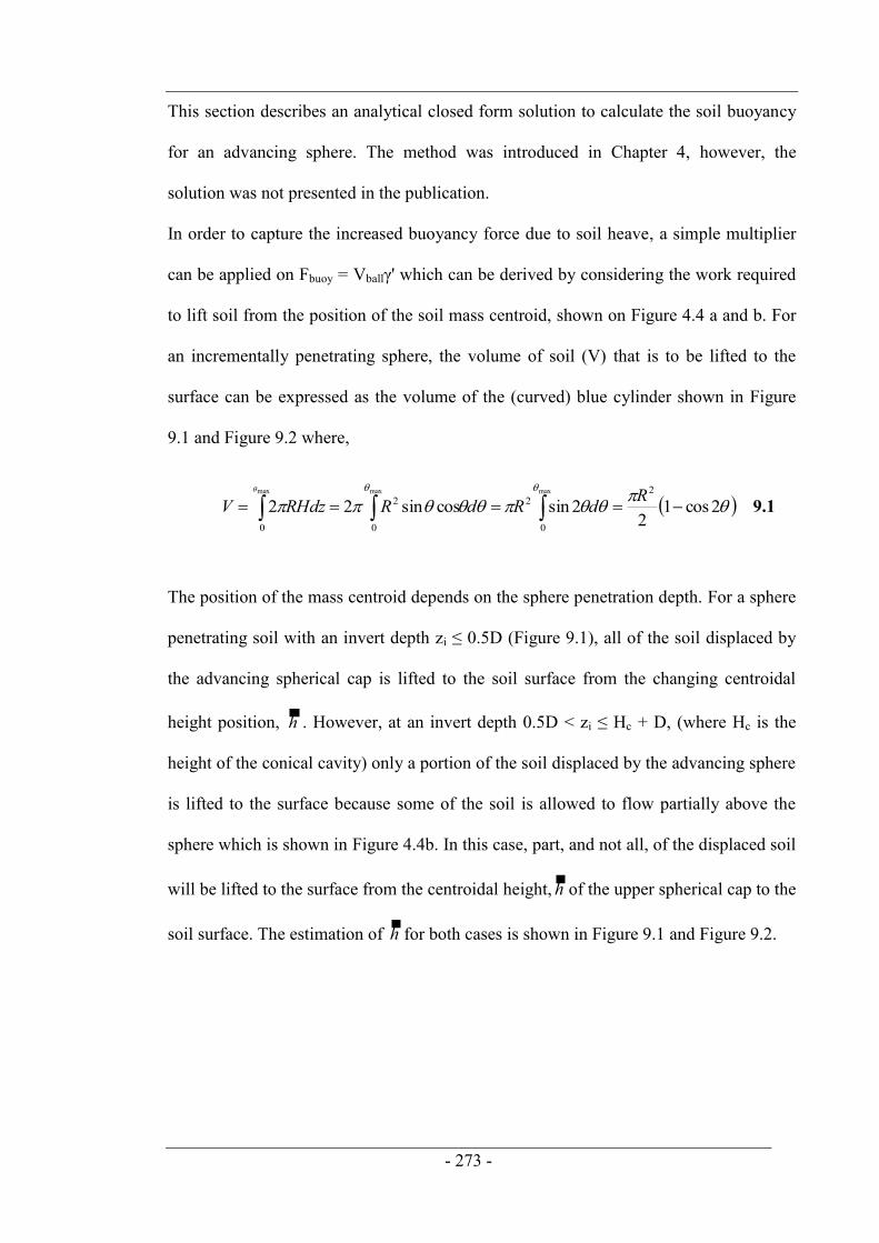
- 273 -
This section describes an analytical closed form solution to calculate the soil buoyancy
for an advancing sphere. The method was introduced in Chapter 4, however, the
solution was not presented in the publication.
In order to capture the increased buoyancy force due to soil heave, a simple multiplier
can be applied on Fbuoy = Vballγ' which can be derived by considering the work required
to lift soil from the position of the soil mass centroid, shown on Figure 4.4 a and b. For
an incrementally penetrating sphere, the volume of soil (V) that is to be lifted to the
surface can be expressed as the volume of the (curved) blue cylinder shown in Figure
9.1 and Figure 9.2 where,
2cos12
2sincossin222
0
2
0
2
0
maxmaxmax
RdRdRRHdzV 9.1
The position of the mass centroid depends on the sphere penetration depth. For a sphere
penetrating soil with an invert depth zi ≤ 0.5D (Figure 9.1), all of the soil displaced by
the advancing spherical cap is lifted to the soil surface from the changing centroidal
height position, h . However, at an invert depth 0.5D < zi ≤ Hc + D, (where Hc is the
height of the conical cavity) only a portion of the soil displaced by the advancing sphere
is lifted to the surface because some of the soil is allowed to flow partially above the
sphere which is shown in Figure 4.4b. In this case, part, and not all, of the displaced soil
will be lifted to the surface from the centroidal height, h of the upper spherical cap to the
soil surface. The estimation of h for both cases is shown in Figure 9.1 and Figure 9.2.

- 274 -
Figure 9.1. The formulation of the centroidal height for an invert depth < 0.5D
Figure 9.2. The formulation of the centroidal height for an invert depth > 0.5D
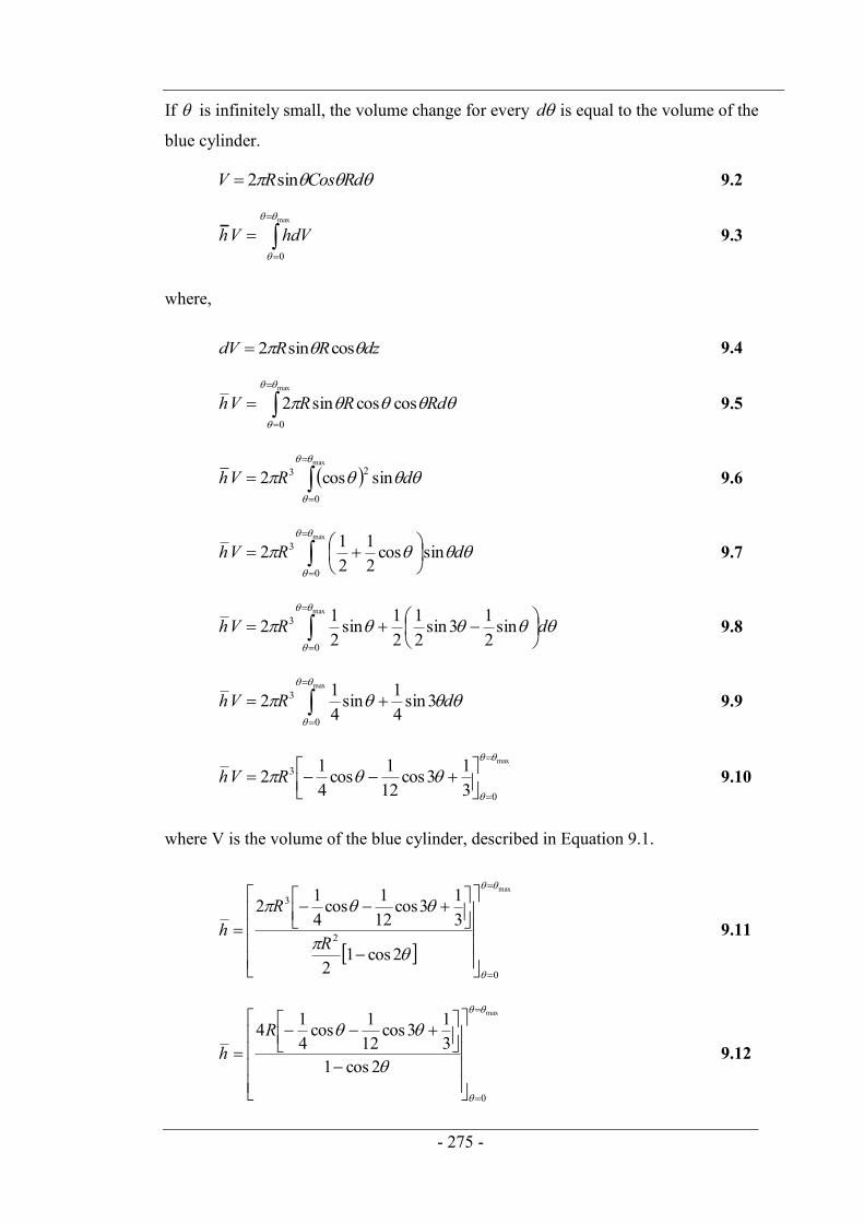
- 275 -
If is infinitely small, the volume change for every d is equal to the volume of the
blue cylinder.
RdCosRV sin2 9.2
max
0
hdVVh 9.3
where,
dzRRdV cossin2 9.4
max
0
coscossin2
RdRRVh 9.5
max
0
23 sincos2
dRVh 9.6
max
0
3 sincos21
212
dRVh 9.7
max
0
3 sin213sin
21
21sin
212
dRVh 9.8
max
0
3 3sin41sin
412
dRVh 9.9
max
0
3
313cos
121cos
412
RVh 9.10
where V is the volume of the blue cylinder, described in Equation 9.1.
max
0
2
3
2cos12
313cos
121cos
412
R
Rh 9.11
max
0
2cos1313cos
121cos
414
Rh 9.12