by mohamed nabil omar
TRANSCRIPT
Comparison between theoretical and practical compression
capacities of deep / long piles
للضغط في الحالتين النظرية والعمليةقدرة تحمل الخوازيق العميقة مقارنة مابين
by
MOHAMED NABIL OMAR
A dissertation submitted in fulfilment
of the requirements for the degree of
MSc. Structural Engineering
at
The British University in Dubai
Prof. Abid Abu Tair November 2017

I
DECLARATION
I warrant that the content of this research is the direct result of my own work and that any use made
in it of published or unpublished copyright material falls within the limits permitted by
international copyright conventions.
I understand that a copy of my research will be deposited in the University Library for permanent
retention.
I hereby agree that the material mentioned above for which I am author and copyright holder may
be copied and distributed by The British University in Dubai for the purposes of research, private
study or education and that The British University in Dubai may recover from purchasers the costs
incurred in such copying and distribution, where appropriate.
I understand that The British University in Dubai may make a digital copy available in the
institutional repository.
I understand that I may apply to the University to retain the right to withhold or to restrict access
to my thesis for a period which shall not normally exceed four calendar years from the
congregation at which the degree is conferred, the length of the period to be specified in the
application, together with the precise reasons for making that application.
_______________________
Mohamed Nabil Omar

II
COPYRIGHT AND INFORMATION TO USERS
The author whose copyright is declared on the title page of the work has granted to the British
University in Dubai the right to lend his/her research work to users of its library and to make partial
or single copies for educational and research use.
The author has also granted permission to the University to keep or make a digital copy for similar
use and for the purpose of preservation of the work digitally.
Multiple copying of this work for scholarly purposes may be granted by either the author, the
Registrar or the Dean of Education only.
Copying for financial gain shall only be allowed with the author’s express permission.
Any use of this work in whole or in part shall respect the moral rights of the author to be
acknowledged and to reflect in good faith and without detriment the meaning of the content, and
the original authorship.

III
ABSTRACT
The rate of build of high-rise buildings has accelerated rapidly, especially in the Arabian
Gulf, over the last few decades, due to rapid urbanization and significant improvements in the field
of the high-rise construction and technology. Many challenges were faced by the engineers in the
design and construction of such buildings. One of the major challenges was the foundation systems,
which are required to ensure the stability of the buildings. The common type of foundation system
which is used in case of high- rise buildings is piles foundation system.
In the most standards and codes of practice such as British Standard and ASTM, the piles
specifications and recommendations are stated for short piles which has a maximum depth range
between 18.0 to 20.0 m. Theoretical equations for pile design, charts and different soil factors and
parameters are based on old studies of short piles behavior. In this research, a comparison was
conducted between the theoretical pile compression capacity which is calculated from the
theoretical equations and the practical pile compression capacity which is derived from the results
of pile’s static load test.
The study covered three different cases of bored piles constructed in U.A.E especially in
Dubai. The piles used in this research have a depth ranging from 30.0 to 65.0 m. This type of piles
is classified in this research as long or deep piles. A finite element model of each pile was modeled
by using PLAXIS 2D software, to compare the practical and theoretical piles capacities. It was
found that the theoretical compression pile capacity is 60 to 70% of the practical pile capacity with
the same specifications (pile diameter and pile depth). As a conclusion of the results, the theoretical
equations which are used to calculate the pile compression capacity can be improved to give results
very near from the practical condition.
Keywords: high-raise buildings, piles, long piles, PLAXIS 2D, piling equipment.

IV
الملخص
يجة النمو الحضاري و الخليج العربي في العقود الاخيرة وذلك نتمعدل بناء المباني العالية قد ازداد بمعدل سريع وخاصة في
النوعية من المباني. التطور الملحوظ في مجال انشاء المباني والابراج العالية. كثير من التحديات قد واجهت المصممين لتلك
الاساسات العميقة تفاع. وتعتبرواحد من التحديات الرئيسة هو الاساسات المستخدمة لتحقيق الاتزان للمباني الشاهقة الار
)الخوازيق( من اكثر انواع الاساسات المستخدمة في حالة المباني شاهقة الارتفاع.
الخوازيق علي في معظم المراجع والاكواد علي سبيل المثال الكود البريطاني والكود الامريكي, يتم تحديد مواصفات وتوصيات
ت البيانية متر. كما ان معظم المعادلات النظرية والرسوما 20الي 18عمقها عن اساس الخوازيق القصيرة والتي لا يتعدي
ا البحث سنقوم ومعاملات التربة المختلفة تعتمد علي دراسات قديمة قد اجريت علي سلوك الخوازيق العادية )القصيرة(. في هذ
ات تحميل فعلية وتلك المحسوبة من نتيجة اختباربمقارنة قدرة تحمل الخوازيق لاحمال الضغط المحسوبة من المعادلات النظرية
للخوازيق العميقة.
لخوازيق المستخدمة الدراسة تغطي ثلاث حالات مختلفة لخوازيق قد تم تنفيذها فعليا في الامارات وخاصة ان دبي. تتراوح اعماق ا
و الطويلة. سيتم اسيتم تصنيف تلك الخوازيق في هذا البحث الي نوعية الخوازيق العميقة متر. 65الي 30في هذا البحث ما بين
لحالة النظرية للمقارنة مابين قدرة تحمل الخوازيق لاحمال الضغط في كلا من ا PLAXIS 2Dنمذجة الخوازيق باستخدام برنامج
60ديمة تساوي تقريبا حسوبة با ستخدام المعادلات النظرية القوالحالة العملية. وكنتيجة لذلك تم وجد ان قدرة تحمل الخوازيق الم
ت النظرية % من قدرة تحمل الخوازيق المحسوبة من نتائج اختبارات التحميل. كنتيجة للدراسة يمكن تعديل المعادلا70الي
لعملية.المستخدمة في حساب قدرة تحمل الخوازيق لاحمال الضغط لتحقيق نتائج اقرب ما يكون من النتائج ا

V
ACKNOWLEDGEMENTS
I would like to express my gratitude to my supervisor Prof. Abid Abu Tair for the useful
comments, remarks and engagement through the learning process of this master thesis.
Furthermore, I would like to thank Prof. Abid Abu Tair for introducing me to the topic as well for
the support on the way.
VI
Table of Contents
COPYRIGHT AND INFORMATION TO USERS .................................................................... ii
ABSTRACT ................................................................................................................................... iii
ACKNOWLEDGEMENTS .......................................................................................................... v
INTRODUCTION.......................................................................................................................... 1
AIMS AND OBJECTIVES ........................................................................................................... 2
CHAPTER 1 - LITERATURE REVIEW .................................................................................... 3
PILES HISTORY .......................................................................................................................... 3
TYPES OF PILE ............................................................................................................................ 4
LARGE DISPLACEMENT PILES – DRIVEN TYPES ................................................ 4
LARGE DISPLACEMENT PILES – DRIVEN AND CAST IN PLACE TYPES ........ 4
SMALL DISPLACEMENT PILES ................................................................................ 4
REPLACEMENT PILES ................................................................................................ 4
SELECTION OF PILE TYPE ...................................................................................................... 5
ULTIMATE LOAD CAPACITY OF SINGLE PILES .............................................................. 9
GENERAL CONSIDERATION ..................................................................................... 9
THE PILE BEHAVIOR UNDER LOAD ....................................................................... 9
1. PILES IN SAND SOIL ......................................................................................... 10
2. PILES IN ROCK SOIL ......................................................................................... 18
1. PREDICTION OF PILE CAPACITY FROM NON-DESTRUCTIVE STATIC LOAD
TEST ..................................................................................................................................... 24
1.1. DAVISSON'S CRITERION .................................................................................. 25
1.2. SHAPE OF THE CURVE ..................................................................................... 26
1.3. LIMITED TOTAL SETTLEMENT METHOD .................................................... 26

VII
1.4. DEBEER'S LOG-LOG METHOD ....................................................................... 27
1.5. BRINCH-HANSEN'S METHOD ......................................................................... 28
1.6. CHIN’S METHOD (the used method in this research) ........................................ 30
PREDICTION OF PILE CAPACITY FROM NON-DESTRUCTIVE BI-DIRECTIONAL
STATIC LOAD TEST (BDSLT) ........................................................................................ 31
A. HIGH LOAD TEST .............................................................................................. 33
B. LOAD TRANSFER TECHNIQUE ...................................................................... 33
EQUIVALENT TOP-DOWN STATIC LOADED LOAD-SETTLEMENT CURVE
FROM THE RESULTS OF A BI-DIRECTIONAL STATIC LOAD TEST
(BDSLT) ................................................................................................................ 34
PROCEDURE A ....................................................................................................... 34
PROCEDURE B ....................................................................................................... 36
LONG / MEGA PILING SYSTEM FOR HIGH-RISE BUILDINGS .................................... 38
INTRODUCTION........................................................................................................................ 38
BEARING BEHAVIORS OF LONG PILE .............................................................................. 39
CHAPTER 2 – RESEARCH METHODOLOGY ..................................................................... 40
CASES OF STUDY...................................................................................................................... 41
CASE 1 _ AL HABTOOR RESIDENCE ..................................................................... 41
PILE DETAIL ........................................................................................................... 42
SOIL LAYERS’ CLASSIFICATIONS ..................................................................... 43
CASE 2 _ BLUEWATER HOSPITALITY ................................................................... 44
PILE DETAIL ........................................................................................................... 45
SOIL LAYERS’ CLASSIFICATIONS ..................................................................... 46
VIII
CASE 3 _ MERSA AL SEEF (GREEK PHASE 3, 4) .................................................. 47
PILE DETAIL ........................................................................................................... 47
SOIL LAYERS’ CLASSIFICATIONS ..................................................................... 49
CHAPTER 3 – RESEARCH RESULTS .................................................................................... 50
NUMERICAL ANALYSIS PROCEDURE ............................................................................... 50
GRAPHICAL BOUNDARIES ..................................................................................... 51
SOIL LAYERS’ CLASSIFICATION AND PARAMETERS ....................................... 52
PILE - SOIL FRICTION RELATIONSHIP ................................................................. 52
CASE 1 _ AL HABTOOR RESIDENCE ................................................................................... 52
A. THEIORTICAL PILE CAPACITY (CASE 1) ...................................................... 52
B. PRACTICAL PILE CAPACITY (CASE 1) .......................................................... 52
C. NUMERICAL PILE CAPACITY (CASE 1) ........................................................ 55
CASE 2 _ BLUEWATER HOSPITALITY ............................................................................... 57
A. THEIORTICAL PILE CAPACITY (CASE 2) ...................................................... 57
B. PRACTICAL PILE CAPACITY (CASE 2) .......................................................... 57
C. NUMERICAL PILE CAPACITY (CASE 2) ........................................................ 59
CASE 3 _ MERSA AL SEEF (GREEK PHASE 3, 4) ............................................................... 61
A. THEIORTICAL PILE CAPACITY (CASE 3) ...................................................... 61
B. PRACTICAL PILE CAPACITY (CASE 3) .......................................................... 61
C. NUMERICAL PILE CAPACITY (CASE 3) ........................................................ 63
CHAPTER 4 – CONCLUSION AND RECOMMENDATIONS............................................. 65
RESULTS DISCUSSION ............................................................................................................ 65
CASE 1 _ AL HABTOOR RESIDENCE ................................................................................... 65
IX
CASE 2 _ BLUEWATER HOSPITALITY ............................................................................... 66
CASE 3 _ MERSA AL SEEF (GREEK PHASE 3, 4) ............................................................... 67
RESEARCH CONCLUSION ..................................................................................................... 68
RESEARCH RECOMMENDATIONS...................................................................................... 70
FURTHER RESEARCH ............................................................................................................. 71
THE METHODOLOGY ............................................................................................................. 71
REFERENCES ............................................................................................................................. 74
Appendix [1] – Numerical Models Output ................................................................................ 77
Numerical Models Output [Case 1] ............................................................................................ 78
Numerical Models Output [Case 2] ............................................................................................ 79
Numerical Models Output [Case 3] ............................................................................................ 80
Appendix [2] – List of Published Papers .................................................................................... 81
X
List of Figures
Figure 1. Bored Cast in Situ - Casing Method ............................................................................... 6
Figure 2. Bored Piles - By using Bentonite Slurry ........................................................................ 7
Figure 3. Flight Auger Piles - CFA ................................................................................................ 8
Figure 4. Load - settlement curve of pile subjected to compression load .................................... 10
Figure 5. Simplified of vertical stress adjacent pile in sand soil ...................................................11
Figure 6. Variation of fb/fs with Ø (Vesic, 1967) ......................................................................... 12
Figure 7. Values of 𝐾𝑠, 𝑡𝑎𝑛∅′𝑎, and 𝑍𝑐/𝑑 for piles in sand ....................................................... 13
Figure 8. Relationship between Nq and Ø (after Berezantzev et al., 1961). ................................ 14
Figure 9. Pile taper factor 𝐹𝜔 (after Nordlund, 1963). ................................................................ 14
Figure 10. Pile bearing capacity factor 𝑁𝑞 ................................................................................. 16
Figure 11. SPT N-values and angle of shearing resistance relationship ...................................... 17
Figure 12. Relation between side wall shear and percantage of socket length ............................ 18
Figure 13. Reduction factors for rock socket shaft friction ......................................................... 19
Figure 14. Reduction factors for discontinuities in rock mass (after Williams and Pells) ........... 20
Figure 15. Mass factor value (after Hobbs) ................................................................................. 21
Figure 16. Pile Static Load Test ................................................................................................... 24
Figure 17. Davisson's Criterion Method ...................................................................................... 26
Figure 18. Shape of The Curve Method ....................................................................................... 27
Figure 19. Determine the Failure Load According to DeBeer's Method ..................................... 28
Figure 20. Determine the Failure Load According to Brinch-Hansen Method............................ 29
Figure 21. Determine the Failure Load According to Chin's Method .......................................... 30
Figure 22. Bi-directional single level load test ............................................................................ 31
Figure 23. Static load test on pile using kentledge method ......................................................... 32
XI
Figure 24. Installation of multiple O-Cells .................................................................................. 33
Figure 25. BDSLT results ............................................................................................................. 35
Figure 26. The equivalent top-down static load test curve .......................................................... 35
Figure 27. Theoretical elastic deformation in BDSLT based on pattern of skin friction stress
development .................................................................................................................................. 36
Figure 28. Theoretical elastic deformation in top-down static load test based on pattern of skin
friction stress development ........................................................................................................... 37
Figure 29. Tallest buildings in the world...................................................................................... 38
Figure 30. Sample of piles recommendation in the soil investigation report............................... 40
Figure 31. Al Habtoor residence .................................................................................................. 41
Figure 32. Al Habtoor residence location .................................................................................... 42
Figure 33. Piles recommendations as per project's soil investigation report ............................... 42
Figure 34. Proposed Bluewater Hospitality Development ........................................................... 44
Figure 35. Piles recommendations as per project's soil investigation report ............................... 45
Figure 36. Mersa Al Seef Development ....................................................................................... 47
Figure 37. Piles recommendations as per project's soil investigation report ............................... 48
Figure 38. Axisymmetric model option ....................................................................................... 50
Figure 39. Graphical boundaries for the pile model .................................................................... 51
Figure 40. Chin's Diagram ........................................................................................................... 54
Figure 41. Pile Model by Using PLAXIS 2D .............................................................................. 55
Figure 42. Pile Load - Settlement Relationship Curve ................................................................ 56
Figure 43. Chin's Diagram ........................................................................................................... 58
Figure 44. Pile Model by Using PLAXIS 2D .............................................................................. 59
Figure 45. Pile Load - Settlement Relationship Curve ................................................................ 60
XII
Figure 46. Chin's Diagram ........................................................................................................... 62
Figure 47. Pile Model by Using PLAXIS 2D .............................................................................. 63
Figure 48. Pile Load - Settlement Relationship Curve ................................................................ 64
Figure 49. Pile Capacities _ Case 1 .............................................................................................. 66
Figure 50. Pile Capacities _ Case 2 .............................................................................................. 67
Figure 51. Pile Capacities _ Case 2 .............................................................................................. 68
Figure 52. Research Results ......................................................................................................... 69
Figure 53. Modified Pile Load - Settlement Relationship Curve................................................. 72
Figure 54. Modified Pile Model by Using PLAXIS 2D .............................................................. 72
Figure 55. Further research results ............................................................................................... 73

XIII
List of Tables
Table 1. The coefficient of the soil horizontal stress, 𝐾𝑆 ............................................................. 16
Table 2. The friction angle between the soil and pile with various interface conditions per
Kulhawy (1984). ........................................................................................................................... 17
Table 3. Mass factor j value with respect to RQD and the discontinuity spacing. ....................... 20
Table 4. Ultimate end bearing resistance of piles in weak mudstones, siltstones and sandstones 22
Table 5. Ultimate base resistance of piles in rock soil in terms of RQD ...................................... 23
Table 6. Pile details ...................................................................................................................... 42
Table 7. Soil layers' classifications ............................................................................................... 43
Table 8. Typical values of modulus of elasticity for different types of soils ................................ 43
Table 9. Bluewater Hospitality Buildings’ Details ....................................................................... 44
Table 10. Pile Details. ................................................................................................................... 45
Table 11. Soil layers' classifications ............................................................................................. 46
Table 12. Pile Details .................................................................................................................... 47
Table 13. Soil layers' classifications ............................................................................................. 49
Table 14. Al Habtoor Residence _ Bi-directional static load test results ..................................... 53
Table 15. Bluewater Hospitality _ Static load test results ............................................................ 57
Table 16. MERSA AL SEEF (GREEK PHASE 3, 4) _ bi-directional static load test results ...... 61
Table 17. Theoretical, practical and numerical pile capacities _ Case 1 ...................................... 65
Table 18. Theoretical, practical and numerical pile capacities _ Case 2 ...................................... 66
Table 19. Theoretical, practical and numerical pile capacities _ Case 3 ...................................... 67
Table 20. Research results ............................................................................................................ 69
Table 21. Further research results ................................................................................................. 73
XIV
List of Abbreviations
𝑃𝑆𝑈 = ultimate pile skin friction resistance
𝑃𝐵𝑈 = ultimate pile end bearing resistance
𝑊𝑃 = pile weight
𝐴𝑏 = Cross sectional area
𝐶 = Cohesion of the soil
𝜎𝑣𝑏 = Vertical stress of the soil at the level of the pile’s base
𝛾 = Soil unit weight
𝑑 = Pile diameter
𝑁𝑐, 𝑁𝑞, 𝑁𝛾 = Soil bearing capacity factors
𝜎′𝑣 = effective vertical stress along pile shaft
𝜎′𝑣𝑏 = effective vertical stress at the pile base level
𝐹𝜔 = correction factor for tapered pile (=1.0 for uniform diameter pile)
𝜎′𝑣0 = the effective soil overburden pressure at the pile base level
𝑁𝑞 = pile bearing capacity factor
𝐴𝑏 = the area of the pile base “cross sectional area”
𝐾𝑠 = coefficient of the soil horizontal stress
𝛿 = friction angle between the pile & soil
𝐴𝑠 = the area of the pile shaft
𝛼 = reduction factor related to 𝑞𝑢𝑐
𝛽 = correction factor related to the discontinuity spacing in the rock mass
𝛿 = elastic deformation of the pile
𝑃 = applied load
𝐿 = pile length
𝐸 = elastic modulus of the pile’s material
𝐴 = cross sectional area of the pile
𝑄𝑢 = ultimate pile capacity
𝛿𝑢 = pile displacement at failure
𝑄𝑢 = ultimate pile capacity
∆ = pile displacement
1
INTRODUCTION
In the last two decades the high rise buildings construction has been significantly improved.
In addition, the construction tools and equipment have been developed to be more effective and to
provide the ability to construct such high rise buildings. The common foundation system which is
used in case of high rise buildings is the piling foundation system. Recently the construction of
piling foundation system has been improved to achieve depths which were impossible to reached
before, by using the advanced piling machines.
Practically and based on actual case of studies, it has been found that there is a big
difference between the calculated pile capacity based on the results of static load tests and the
estimated pile capacities obtained using classical theoretical equations. These differences are
increased in case of the increased of pile depths. This research will compare between the theoretical
pile capacity and the practical pile capacity. Also numerical model will be developed to identify a
more accurate numerical pile capacity.
Three case studies will be discussed in this research, these cases are from real projects that
have been constructed in Dubai. The projects data such as soil investigation reports, piling
drawings and the results of piles' static load test have been collected from the projects' consultant
for further development and research.
2
AIMS AND OBJECTIVES
The aim of this research is to conduct a comparison between theoretical pile capacity
derived using classical soil mechanics equations with real static test results of piles constructed in
Dubai and to propose more optimum design models.
The objectives of this research are as follow;
1. Calculate the practical pile capacity from the results of static load test in each case
of study.
2. Model the selected pile of each case of study by using a finite element software,
and estimate the numerical pile capacity by using a prescribed settlement on the
pile head.
3. Comparison between the practical, theoretical and numerical compression pile
capacity will be done to identify the differences.
4. further research to specify the differences between the theoretical pile capacity and
numerical pile capacity, the compassion will be done for pile skin friction resistance
and end bearing resistance separately. This further research will be done based on
the developed pile model.
3
CHAPTER 1 - LITERATURE REVIEW
A pile is a structural element whose function is to transfer the superstructure loads through
weak soil layers to the hard soil strata or the rock layers. Another use of the pile which is the
resistance to the uplift force, in case of high rise building subjected to overturning force or to
support a structure has a low weight compared to the uplift force which is generated from high
water table. This type of piles is called tension piles. Piles are mainly used to resist a compression
forces from the superstructure and in this case the piles are classified as a comparison piles.
PILES HISTORY
Driven piles as type of structures foundation is one of the oldest types which used to ensure
the stability of different types of structures like buildings and bridges. In U.K there are so many
examples of timber piles used to support different bridges constructed by the Romans. In the old
ages, piles of timber has been used in the construction of great monasteries’s foundations which
has been constructed in Europe. In China, the wooden piles were used by the builders especially
the bridges’ builders of the Han Dynasty (200 BC to AD 200). Based on that, the rules have been
established in the beginning of using the piles foundation by which the pile capacity was
determined from its resistance to the driving force by a hammer of known weight and with a known
height of drop.
Timber, as a result of its quality joined with delicacy, strength and simplicity of cutting and
taking care of, remained the main material utilized for heaping until nearly late circumstances. It
was supplanted by concrete and steel simply because these more up to date materials could be
manufactured into units that were equipped for managing compressive, twisting and ductile powers
a long ways past the limit of a timber heap of like measurements. Concrete piles has been devolved
to provide the ability to construct the piles in a drilled holes (bored piles) in situations where noise,
vibration and ground heave had to be avoided.
Reinforced concrete piles, which were developed as structural elements in the previous two
centuries, and it has been widely used instead of timber piles. The concrete piles can be formed in
different shapes to suit the structure requirement and the imposed load. The durability and the
reaction with the different types of soil layers gives the concrete another advantage. Steel piles are
a common type of piles especially in marine structure due to the ease of the installation. Nowadays
there are different types of paints and chemicals used to improve the steel resistance to corrosion
and can increase the steel piles’ durability.
4
TYPES OF PILE
Most of standard codes classified the types of piles to three main categories, the first
category is the large displacement piles which include solid or hollow sections closed at their end,
driven or caste in place into the ground. The second category is small displacement piles which
have the same function of the first category but with small sections. This types includes steel rolled
H or I section. The third type is replacement piles, these types constructed by replacing the soil
by boring using different types of the drilling techniques. Then filling the bore by the used pile
material such as concrete, timber or steel.
LARGE DISPLACEMENT PILES – DRIVEN TYPES
1. Timber with different section shapes.
2. Precast concrete soiled or tubular sections.
3. Restressed concrete piles.
4. Steel tubes or boxes with closed end.
LARGE DISPLACEMENT PILES – DRIVEN AND CAST IN PLACE TYPES
1. Steel tubes driven after placing concrete.
2. Precast concrete sections filled by concrete.
3. Steel shell driven and then filled with concrete.
SMALL DISPLACEMENT PILES
1. Precast concrete tubular section driven with open end.
2. Pre-stressed concrete tubular section driven with open end.
3. Steel H sections.
4. Steel tube or box section driven with open end and soil removed as required.
REPLACEMENT PILES
1. Concrete bored piles.
2. Cement mortar casted in the drilled hole.
3. Steel sections placed into drilled hole.
The selection criteria of the used pile type depend on different factors, the major factor is
the type of the soil layers, where driven piles can be easily used in weak soil layers compared to
replacement piles used with hard soil layers. In the second place, there are important factors such
as the superstructure's material, the availability of the used pile materials, the used pile machines
and techniques and the requirements for pile durability.
5
SELECTION OF PILE TYPE
The selection of the pile type depends on three major factors; the first factor is the
LOCATION AND THE TYPE OF THE STRUCTURE. The second factor is the GROUND
CONDITIONS such as cohesive and loose soil. This factor effect on the choosing of the pile
material and the installation technique. For example, the drilling of piles in cohesive soil layers
can be performed without using a bentonite slurry to protect the borehole side from failure unlike
the drilling in the loose soil or clay layers.
The third factor is the DURABILITY of the piles, this factor effect on the selecting of the
pile material. For example, in some countries the using of wood as a pile foundation can be cheap
compared to any other material like steel and reinforced concrete. But in terms of durability the
using of reinforced concrete or steel instead of wood as a pile foundation can be considered as a
durable option.
6
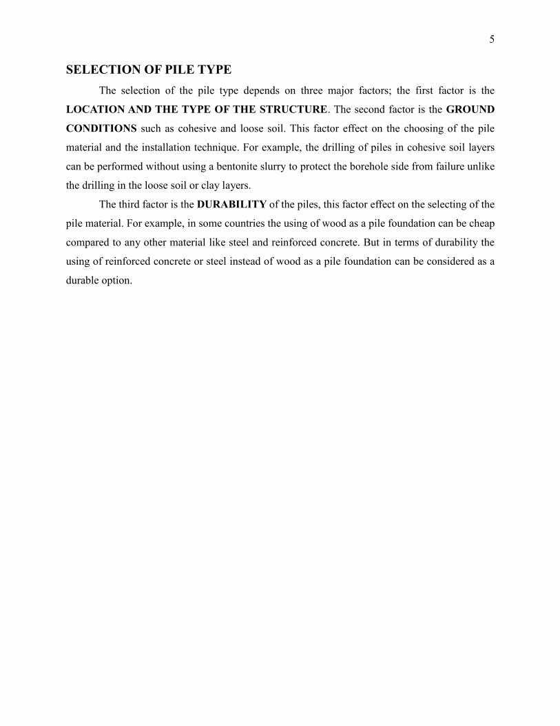
Figure 1. Bored Cast in Situ - Casing Method
7
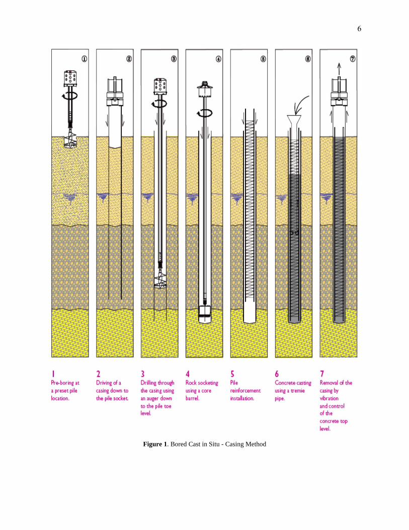
Figure 2. Bored Piles - By using Bentonite Slurry
8
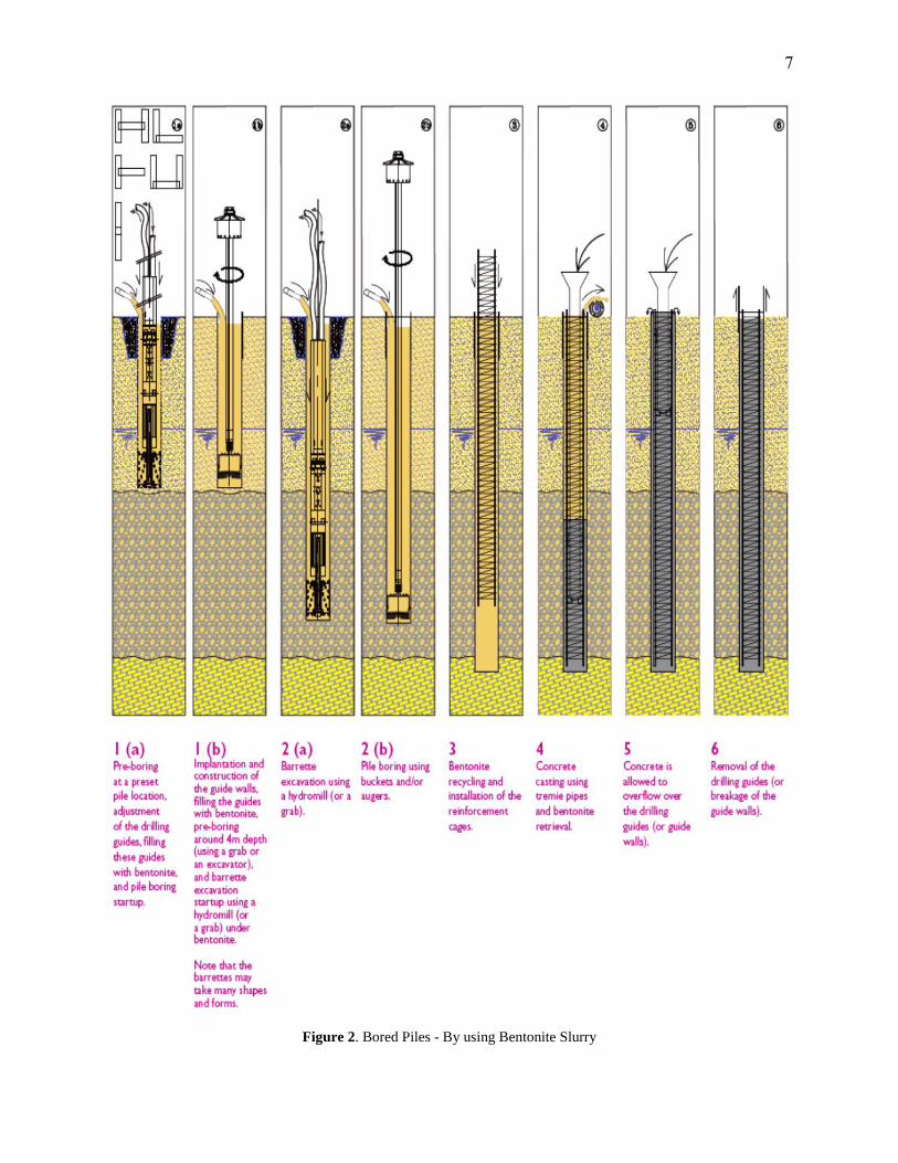
Figure 3. Flight Auger Piles - CFA
9
ULTIMATE LOAD CAPACITY OF SINGLE PILES
GENERAL CONSIDERATION
This section will cover the geotechnical method to estimate the compression pile capacity.
In the past time, much research work was done to express a method based on the practical soil
mechanics theory. For example, the calculation of skin friction on a pile shaft was based on a
simple relationship between the effective overburden pressure, the drained angle of shearing
resistance of the soil and the coefficient of earth pressure at rest, but they realized through the
results of the practical tests and researches that the pile’s skin friction resistance should modified
by a factor takes into consideration the installation technique of the pile.
In the same way, the calculation of the pile end bearing resistance was based on the soil
shearing resistance at the pile toe level, but the researcher recognized the importance of the pile
settlement at the pile’s working load. A methods have developed to estimate the pile’s settlement,
based on elastic theory and considering the skin friction transfer between the pile surface and
surrounded soil.
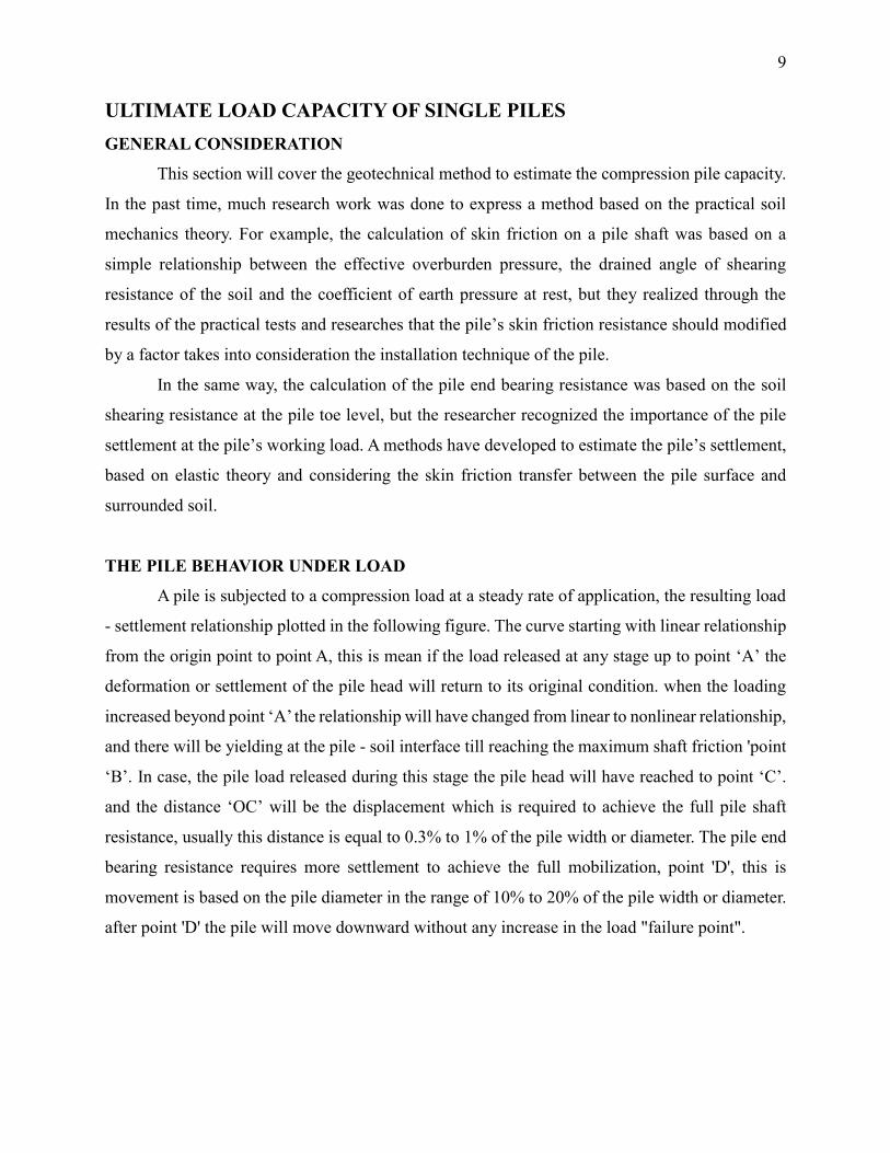
THE PILE BEHAVIOR UNDER LOAD
A pile is subjected to a compression load at a steady rate of application, the resulting load
- settlement relationship plotted in the following figure. The curve starting with linear relationship
from the origin point to point A, this is mean if the load released at any stage up to point ‘A’ the
deformation or settlement of the pile head will return to its original condition. when the loading
increased beyond point ‘A’ the relationship will have changed from linear to nonlinear relationship,
and there will be yielding at the pile - soil interface till reaching the maximum shaft friction 'point
‘B’. In case, the pile load released during this stage the pile head will have reached to point ‘C’.
and the distance ‘OC’ will be the displacement which is required to achieve the full pile shaft
resistance, usually this distance is equal to 0.3% to 1% of the pile width or diameter. The pile end
bearing resistance requires more settlement to achieve the full mobilization, point 'D', this is
movement is based on the pile diameter in the range of 10% to 20% of the pile width or diameter.
after point 'D' the pile will move downward without any increase in the load "failure point".
10
1. PILES IN SAND SOIL
The ultimate pile capacity, Pu, of a single pile is equal to the summation of the ultimate
skin friction and end bearing resistances, less the pile weight;
𝑃𝑈 = 𝑃𝑆𝑈 + 𝑃𝐵𝑈 − 𝑊𝑃 ….. Eq. (1)
Where,
𝑃𝑆𝑈 = ultimate pile skin friction resistance
𝑃𝐵𝑈 = ultimate pile end bearing resistance
𝑊𝑃 = pile weight
For sand soil, there was an empirical method developed and reviewed by Vesic (1967),
𝑃𝑈 = ∫ 𝐶(𝑐𝑎 + 𝜎𝑣 𝐾𝑠 tan ∅𝑎
𝐿
0
) 𝑑𝑧 + 𝐴𝑏 (𝑐𝑁𝑐 + 𝜎𝑣𝑏𝑁𝑞 + 0.5 𝛾𝑑𝑁𝛾)𝑤 ….. Eq. (2)
Where,
𝐴𝑏 = Cross sectional area
𝐶 = Cohesion of the soil
𝜎𝑣𝑏 = Vertical stress of the soil at the level of the pile’s base
𝛾 = Soil unit weight
Figure 4. Load - settlement curve of pile subjected to compression load
11
𝑑 = Pile diameter
𝑁𝑐, 𝑁𝑞, 𝑁𝛾 = Soil bearing capacity factors
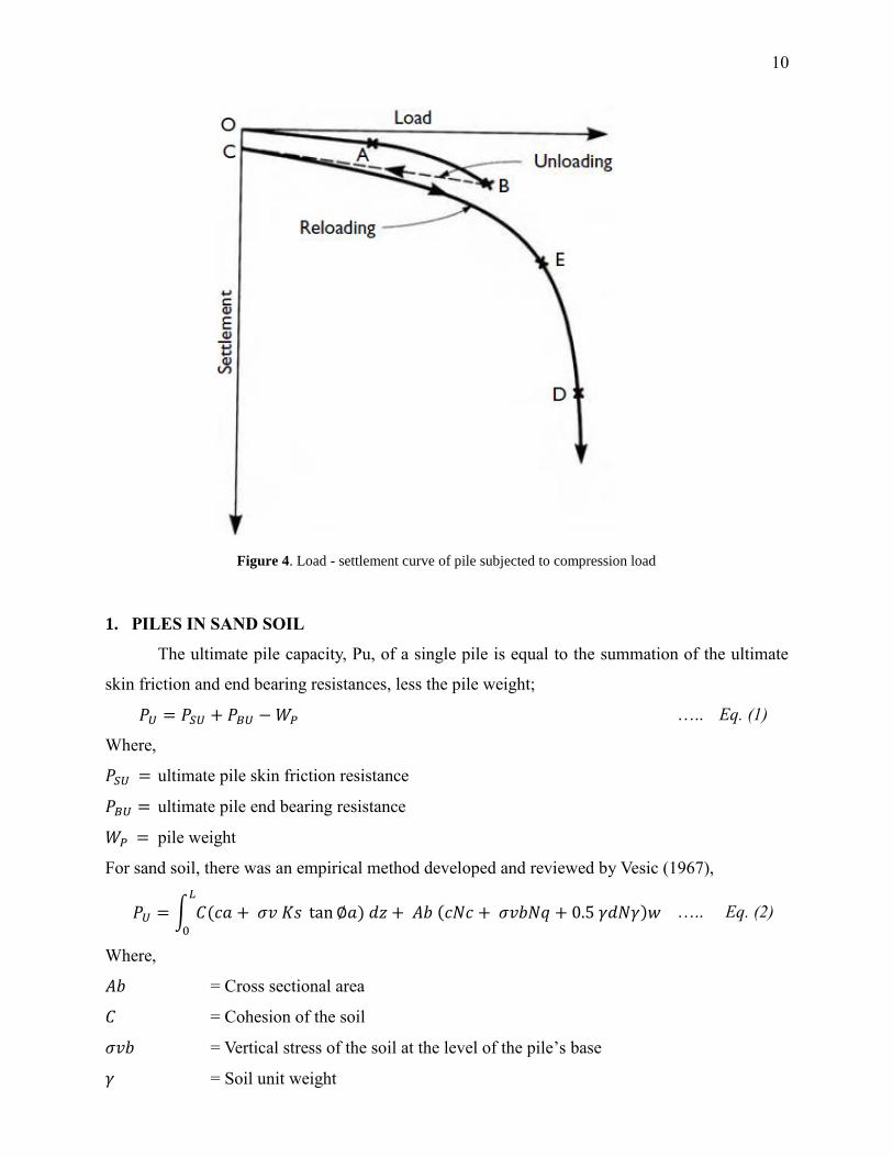
Another method to calculate the ultimate pile capacity in sand soil (Broms, 1966; Nordlund,
1963) assume that the vertical soil stresses 𝜎𝑣 and 𝜎𝑣𝑏 in Eq. 2 are the effective vertical stresses
caused by the soil overburden. However, a research by Vesic (1967) and Kerisel (1961) indicated
that the pile shaft and base resistances are not increasing linearly with the depth, but reached a
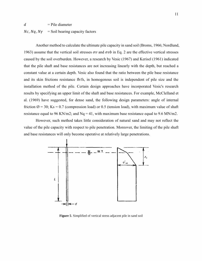
constant value at a certain depth. Vesic also found that the ratio between the pile base resistance
and its skin frictions resistance fb/fs, in homogenous soil is independent of pile size and the
installation method of the pile. Certain design approaches have incorporated Vesic's research
results by specifying an upper limit of the shaft and base resistances. For example, McClelland et
al. (1969) have suggested, for dense sand, the following design parameters: angle of internal
friction Ø = 30; Ks = 0.7 (compression load) or 0.5 (tension load), with maximum value of shaft
resistance equal to 96 KN/m2; and Nq = 41, with maximum base resistance equal to 9.6 MN/m2.
However, such method takes little consideration of natural sand and may not reflect the
value of the pile capacity with respect to pile penetration. Moreover, the limiting of the pile shaft
and base resistances will only become operative at relatively large penetrations.
Figure 5. Simplified of vertical stress adjacent pile in sand soil
12
In Eq. 2, if the pile and soil adhesion 𝑐𝑎 and the term 𝑐𝑁𝑐 are taken equal to zero, and the
term 0.5 is neglected because of the small value compared to Nq term, the ultimate pile capacity
load of single pile in sand can be expressed as per the following equation:
𝑃𝑈 = ∫ 𝐹𝜔 𝐶 𝜎′𝑣 𝐾𝑠 tan ∅′𝑎
𝐿
0
. 𝑑𝑧 + 𝐴𝑏 𝜎′𝑣𝑏𝑁𝑞 . 𝑤 ….. Eq. (3)
Where,
𝜎′𝑣 = effective vertical stress along pile shaft
𝜎′𝑣𝑏 = effective vertical stress at the pile base level
𝐹𝜔 = correction factor for tapered pile (=1.0 for uniform diameter pile)
Figure 6. Variation of fb/fs with Ø (Vesic, 1967)
13
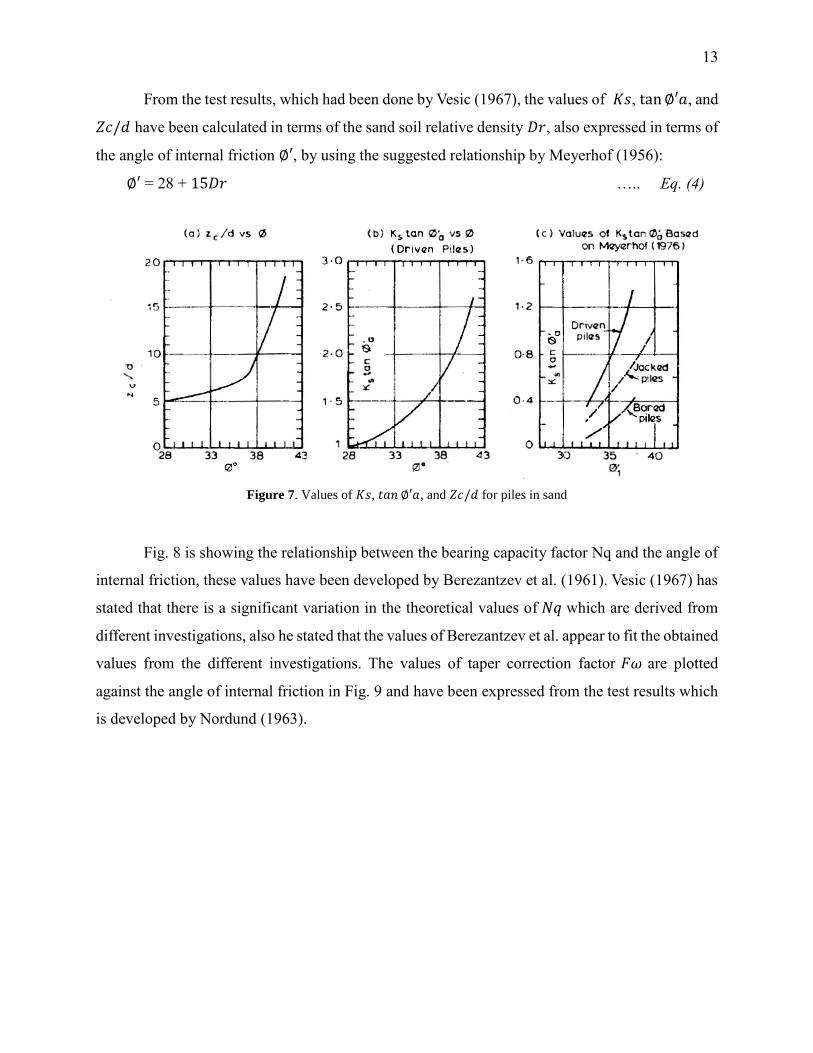
From the test results, which had been done by Vesic (1967), the values of 𝐾𝑠, tan ∅′𝑎, and
𝑍𝑐/𝑑 have been calculated in terms of the sand soil relative density 𝐷𝑟, also expressed in terms of
the angle of internal friction ∅′, by using the suggested relationship by Meyerhof (1956):
∅′ = 28 + 15𝐷𝑟 ….. Eq. (4)
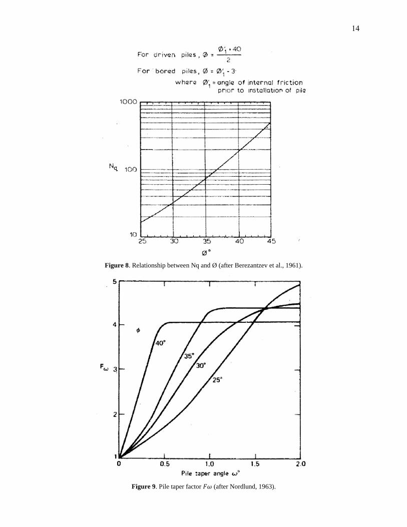
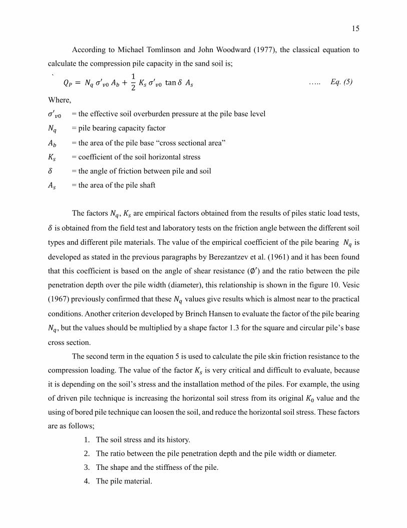
Fig. 8 is showing the relationship between the bearing capacity factor Nq and the angle of
internal friction, these values have been developed by Berezantzev et al. (1961). Vesic (1967) has
stated that there is a significant variation in the theoretical values of 𝑁𝑞 which are derived from
different investigations, also he stated that the values of Berezantzev et al. appear to fit the obtained
values from the different investigations. The values of taper correction factor 𝐹𝜔 are plotted
against the angle of internal friction in Fig. 9 and have been expressed from the test results which
is developed by Nordund (1963).
Figure 7. Values of 𝐾𝑠, 𝑡𝑎𝑛 ∅′𝑎, and 𝑍𝑐/𝑑 for piles in sand
14
Figure 8. Relationship between Nq and Ø (after Berezantzev et al., 1961).
Figure 9. Pile taper factor 𝐹𝜔 (after Nordlund, 1963).
15
According to Michael Tomlinson and John Woodward (1977), the classical equation to
calculate the compression pile capacity in the sand soil is;
` 𝑄𝑃 = 𝑁𝑞 𝜎′𝑣0 𝐴𝑏 +
1
2 𝐾𝑠 𝜎′𝑣0 tan 𝛿 𝐴𝑠 ….. Eq. (5)
Where,
𝜎′𝑣0 = the effective soil overburden pressure at the pile base level
𝑁𝑞 = pile bearing capacity factor
𝐴𝑏 = the area of the pile base “cross sectional area”
𝐾𝑠 = coefficient of the soil horizontal stress
𝛿 = the angle of friction between pile and soil
𝐴𝑠 = the area of the pile shaft
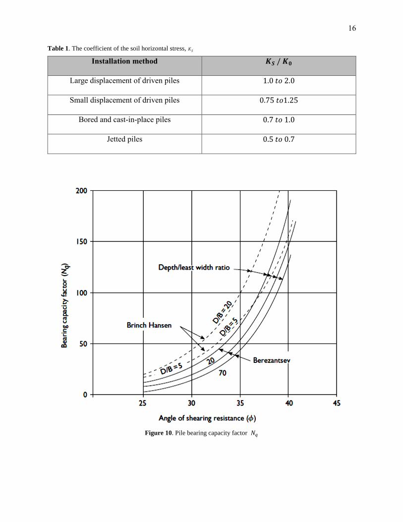
The factors 𝑁𝑞, 𝐾𝑠 are empirical factors obtained from the results of piles static load tests,
𝛿 is obtained from the field test and laboratory tests on the friction angle between the different soil
types and different pile materials. The value of the empirical coefficient of the pile bearing 𝑁𝑞 is
developed as stated in the previous paragraphs by Berezantzev et al. (1961) and it has been found
that this coefficient is based on the angle of shear resistance (∅′) and the ratio between the pile
penetration depth over the pile width (diameter), this relationship is shown in the figure 10. Vesic
(1967) previously confirmed that these 𝑁𝑞 values give results which is almost near to the practical
conditions. Another criterion developed by Brinch Hansen to evaluate the factor of the pile bearing
𝑁𝑞, but the values should be multiplied by a shape factor 1.3 for the square and circular pile’s base
cross section.
The second term in the equation 5 is used to calculate the pile skin friction resistance to the
compression loading. The value of the factor 𝐾𝑠 is very critical and difficult to evaluate, because
it is depending on the soil’s stress and the installation method of the piles. For example, the using
of driven pile technique is increasing the horizontal soil stress from its original 𝐾0 value and the
using of bored pile technique can loosen the soil, and reduce the horizontal soil stress. These factors
are as follows;
1. The soil stress and its history.
2. The ratio between the pile penetration depth and the pile width or diameter.
3. The shape and the stiffness of the pile.
4. The pile material.
16
Table 1. The coefficient of the soil horizontal stress, 𝐾𝑆
Installation method 𝑲𝑺 / 𝑲𝟎
Large displacement of driven piles 1.0 𝑡𝑜 2.0
Small displacement of driven piles 0.75 𝑡𝑜1.25
Bored and cast-in-place piles 0.7 𝑡𝑜 1.0
Jetted piles 0.5 𝑡𝑜 0.7
Figure 10. Pile bearing capacity factor 𝑁𝑞
17
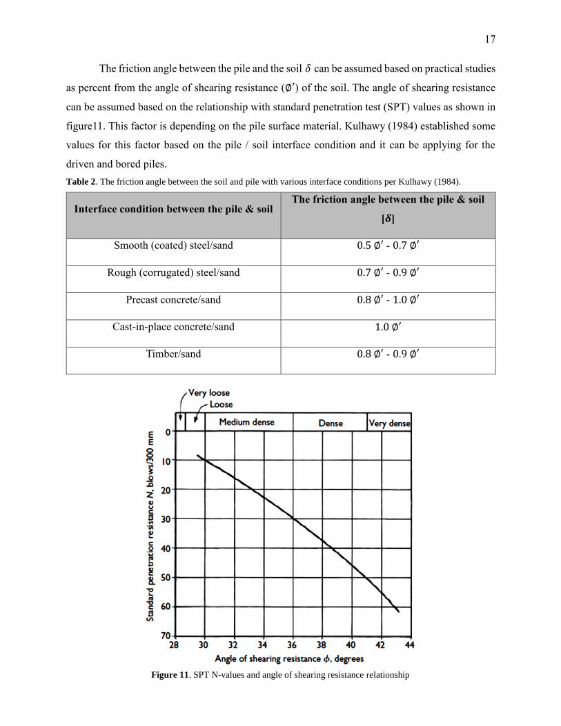
The friction angle between the pile and the soil 𝛿 can be assumed based on practical studies
as percent from the angle of shearing resistance (∅′) of the soil. The angle of shearing resistance
can be assumed based on the relationship with standard penetration test (SPT) values as shown in
figure11. This factor is depending on the pile surface material. Kulhawy (1984) established some
values for this factor based on the pile / soil interface condition and it can be applying for the
driven and bored piles.
Table 2. The friction angle between the soil and pile with various interface conditions per Kulhawy (1984).
Interface condition between the pile & soil The friction angle between the pile & soil
[𝜹]
Smooth (coated) steel/sand 0.5 ∅′ - 0.7 ∅′
Rough (corrugated) steel/sand 0.7 ∅′ - 0.9 ∅′
Precast concrete/sand 0.8 ∅′ - 1.0 ∅′
Cast-in-place concrete/sand 1.0 ∅′
Timber/sand 0.8 ∅′ - 0.9 ∅′
Figure 11. SPT N-values and angle of shearing resistance relationship
18
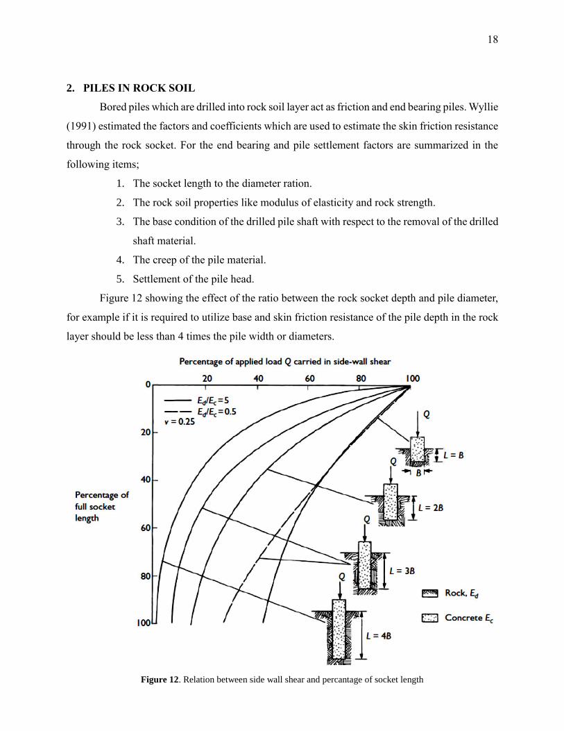
2. PILES IN ROCK SOIL
Bored piles which are drilled into rock soil layer act as friction and end bearing piles. Wyllie
(1991) estimated the factors and coefficients which are used to estimate the skin friction resistance
through the rock socket. For the end bearing and pile settlement factors are summarized in the
following items;
1. The socket length to the diameter ration.
2. The rock soil properties like modulus of elasticity and rock strength.
3. The base condition of the drilled pile shaft with respect to the removal of the drilled
shaft material.
4. The creep of the pile material.
5. Settlement of the pile head.
Figure 12 showing the effect of the ratio between the rock socket depth and pile diameter,
for example if it is required to utilize base and skin friction resistance of the pile depth in the rock
layer should be less than 4 times the pile width or diameters.
Figure 12. Relation between side wall shear and percantage of socket length

19
The condition of the pile's surrounding soil layers is very important factor, and it has a
significant impact on the pile skin friction. For example, the drilling in clayey shale, or clayey
weathered marl cause a softening in borehole wall, as well as, the using of the bentonite slurry in
the drilling process has the same impact on the pile skin friction. This impact can be avoided by
using a temporary casing technique in the installation of the pile, the casing should be extending
to the head of rock soil layer. Wyllie (1991) stated that if the bentonite slurry used in the drilling
process of the pile, the rock friction resistance should be reduced by 25% compared to clean rock
socket, unless pile load test done to verify the actual value of the friction resistance.
The shaft resistance of the pile in the rock soil, depends on the bond between the pile
material which is concrete and the rock soil. The bond between the concrete and the rock soil is
based on the unconfined compression strength of the rock soil, the rock socket bond stress has
been developed by Horvarth (1978), Rosenberg and Journeaux (1976), and Williams and Pells
(1981). The ultimate skin friction resistance 𝑓𝑠 , in the rock soil can be calculated by the following
equation;
𝑓𝑠 = 𝛼 𝛽 𝑞𝑢𝑐 ….. Eq. (6)
Where,
𝛼 = reduction factor related to 𝑞𝑢𝑐 as shown in figure 13.
𝛽 = correction factor related to the discontinuity spacing in the rock mass as shown in figure 14.
Figure 13. Reduction factors for rock socket shaft friction
20
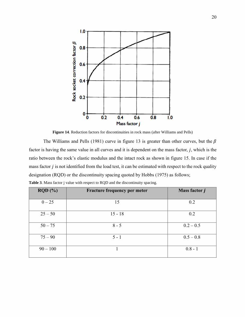
The Williams and Pells (1981) curve in figure 13 is greater than other curves, but the 𝛽
factor is having the same value in all curves and it is dependent on the mass factor, 𝑗, which is the
ratio between the rock’s elastic modulus and the intact rock as shown in figure 15. In case if the
mass factor 𝑗 is not identified from the load test, it can be estimated with respect to the rock quality
designation (RQD) or the discontinuity spacing quoted by Hobbs (1975) as follows;
Table 3. Mass factor j value with respect to RQD and the discontinuity spacing.
RQD (%) Fracture frequency per meter Mass factor 𝒋
0 – 25 15 0.2
25 – 50 15 - 18 0.2
50 – 75 8 - 5 0.2 – 0.5
75 – 90 5 - 1 0.5 – 0.8
90 – 100 1 0.8 - 1
Figure 14. Reduction factors for discontinuities in rock mass (after Williams and Pells)
21
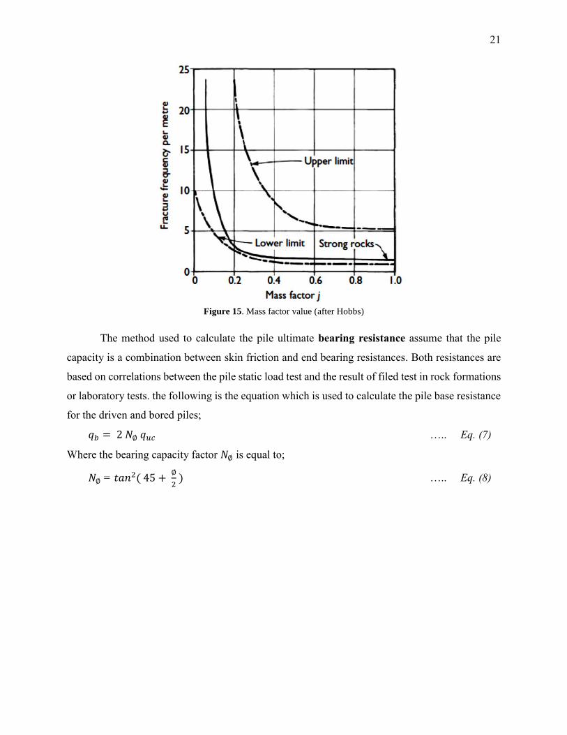
The method used to calculate the pile ultimate bearing resistance assume that the pile
capacity is a combination between skin friction and end bearing resistances. Both resistances are
based on correlations between the pile static load test and the result of filed test in rock formations
or laboratory tests. the following is the equation which is used to calculate the pile base resistance
for the driven and bored piles;
𝑞𝑏 = 2 𝑁∅ 𝑞𝑢𝑐 ….. Eq. (7)
Where the bearing capacity factor 𝑁∅ is equal to;
𝑁∅ = 𝑡𝑎𝑛2( 45 + ∅
2 ) ….. Eq. (8)
Figure 15. Mass factor value (after Hobbs)

22
The following table shows the variations in the value of bearing resistance factor 𝑁∅ for driven
and bored piles in different types of rock soil;
Table 4. Ultimate end bearing resistance of piles in weak mudstones, siltstones and sandstones
Description of
rock Pile type
Plate or
pile
diameter
[mm]
Observed
bearing
pressure at
failure
[MN/m2]
Calculated 𝑵∅
Mudstone /
siltstone
moderately weak
Bored pile 900 5.6 0.25
Mudstone, highly
to moderately
weathered weal
Plate test 457 9.2 1.25
Cretaceous
mudstone weak,
weathered, clayey
Bored pile 670 6.8 3.0
Weak carbonate
siltstone/sandstone Driven 762 5.11 1.5
Calcareous
sandstone weak Driven tube 200 3.0 1.2
Sandstone, weak to
moderately weak Driven 275
19 (from
dynamic pile
test)
1.75
The pile bearing resistance in weak rock soil depends on the drilling techniques. The use
of percussive drilling equipment causes a formation of a soft sludge material at the bottom level
of the drilled pile shaft. This is not only causing a reduction in the pile’s base resistance, it makes
it difficult to identify the accurate classification of the rock soil and difficult to estimate the soil
parameters at the base level. In case of weathered mudstones, siltstones and shales undisturbed
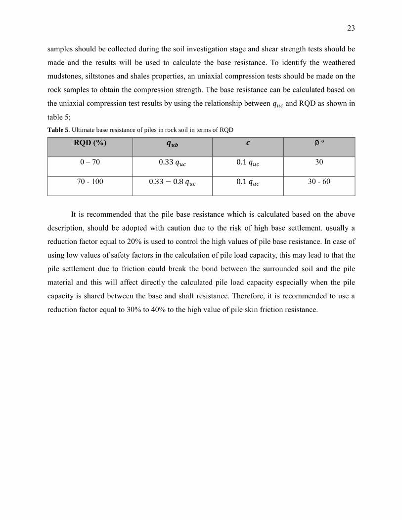
23
samples should be collected during the soil investigation stage and shear strength tests should be
made and the results will be used to calculate the base resistance. To identify the weathered
mudstones, siltstones and shales properties, an uniaxial compression tests should be made on the
rock samples to obtain the compression strength. The base resistance can be calculated based on
the uniaxial compression test results by using the relationship between 𝑞𝑢𝑐 and RQD as shown in
table 5;
Table 5. Ultimate base resistance of piles in rock soil in terms of RQD
RQD (%) 𝒒𝒖𝒃 𝒄 ∅ o
0 – 70 0.33 𝑞𝑢𝑐 0.1 𝑞𝑢𝑐 30
70 - 100 0.33 − 0.8 𝑞𝑢𝑐 0.1 𝑞𝑢𝑐 30 - 60
It is recommended that the pile base resistance which is calculated based on the above
description, should be adopted with caution due to the risk of high base settlement. usually a
reduction factor equal to 20% is used to control the high values of pile base resistance. In case of
using low values of safety factors in the calculation of pile load capacity, this may lead to that the
pile settlement due to friction could break the bond between the surrounded soil and the pile
material and this will affect directly the calculated pile load capacity especially when the pile
capacity is shared between the base and shaft resistance. Therefore, it is recommended to use a
reduction factor equal to 30% to 40% to the high value of pile skin friction resistance.
24
1. PREDICTION OF PILE CAPACITY FROM NON-DESTRUCTIVE
STATIC LOAD TEST
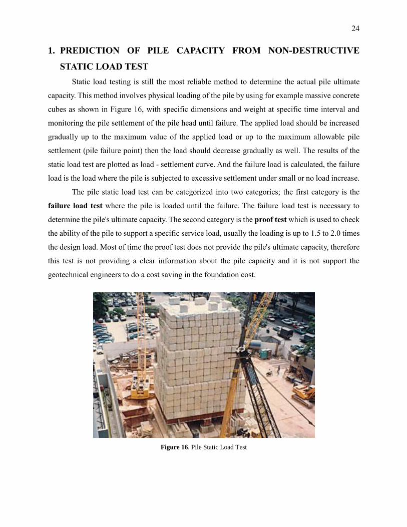
Static load testing is still the most reliable method to determine the actual pile ultimate
capacity. This method involves physical loading of the pile by using for example massive concrete
cubes as shown in Figure 16, with specific dimensions and weight at specific time interval and
monitoring the pile settlement of the pile head until failure. The applied load should be increased
gradually up to the maximum value of the applied load or up to the maximum allowable pile
settlement (pile failure point) then the load should decrease gradually as well. The results of the
static load test are plotted as load - settlement curve. And the failure load is calculated, the failure
load is the load where the pile is subjected to excessive settlement under small or no load increase.
The pile static load test can be categorized into two categories; the first category is the
failure load test where the pile is loaded until the failure. The failure load test is necessary to
determine the pile's ultimate capacity. The second category is the proof test which is used to check
the ability of the pile to support a specific service load, usually the loading is up to 1.5 to 2.0 times
the design load. Most of time the proof test does not provide the pile's ultimate capacity, therefore
this test is not providing a clear information about the pile capacity and it is not support the
geotechnical engineers to do a cost saving in the foundation cost.
Figure 16. Pile Static Load Test
25
Vesic (1977) stated that the scale of the load - settlement curve is based on the elastic
deformation of the pile and is expressed as;
𝛿 =𝑃𝐿 𝐸𝐴⁄ ….. Eq. (9)
Where;
𝛿 = elastic deformation of the pile
P = applied load
L = pile length
E = elastic modulus of the pile’s material
A = cross sectional area of the pile
The following section explain the different methods which are used to extrapolate the
failure load from non-failed load test;
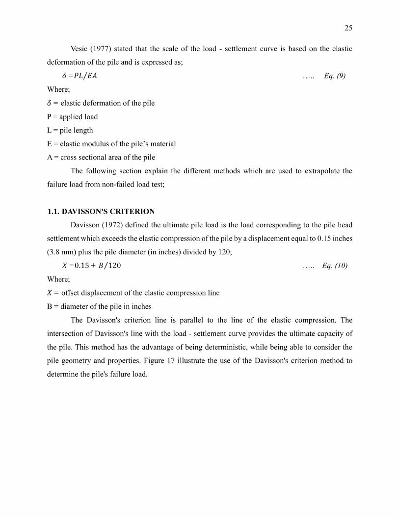
1.1. DAVISSON'S CRITERION
Davisson (1972) defined the ultimate pile load is the load corresponding to the pile head
settlement which exceeds the elastic compression of the pile by a displacement equal to 0.15 inches
(3.8 mm) plus the pile diameter (in inches) divided by 120;
𝑋 =0.15 + 𝐵 120⁄ ….. Eq. (10)
Where;
𝑋 = offset displacement of the elastic compression line
B = diameter of the pile in inches
The Davisson's criterion line is parallel to the line of the elastic compression. The
intersection of Davisson's line with the load - settlement curve provides the ultimate capacity of
the pile. This method has the advantage of being deterministic, while being able to consider the
pile geometry and properties. Figure 17 illustrate the use of the Davisson's criterion method to
determine the pile's failure load.
26
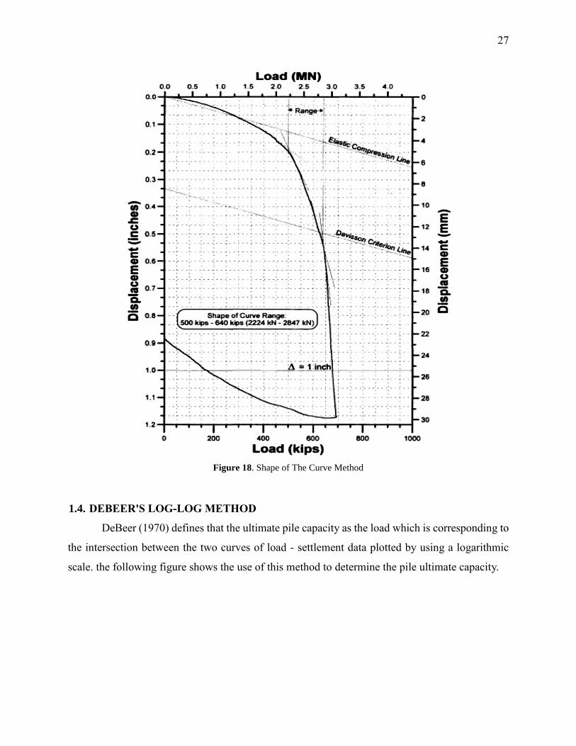
1.2. SHAPE OF THE CURVE
The shape of the curve is an approximation method to determine the failure load or the
ultimate pile capacity from non-failure load test. The failure range is defining for load-settlement
curve that exhibit rapid settlement with slightly increased loads. The piles that experience non-
plunging failure, are difficult to analyze using this method because of the uniform changes in the
slope of the lines drawn tangent to the curve. Figure 18 illustrates the use of the shape of the curve
method to determine the range of the ultimate pile capacity from non-failure static load test.
1.3. LIMITED TOTAL SETTLEMENT METHOD
The limited total settlement method is an approximation method to calculate or determine
the pile ultimate capacity from non-failure load test. The ultimate pile capacity by this method is
defined as the load corresponding to the settlement of 1.0 inch and 0.1 times the pile diameter
(Terzaghi, 1942). The disadvantage of this method is that it is not applicable in many cases. for
example, the elastic deformation of any long steel pile may exceed 1.0 inch and/or 0.1B (pile
diameter) without any plastic deformation in the soil.
Figure 17. Davisson's Criterion Method
27
1.4. DEBEER'S LOG-LOG METHOD
DeBeer (1970) defines that the ultimate pile capacity as the load which is corresponding to
the intersection between the two curves of load - settlement data plotted by using a logarithmic
scale. the following figure shows the use of this method to determine the pile ultimate capacity.
Figure 18. Shape of The Curve Method

28
1.5. BRINCH-HANSEN'S METHOD
Brinch-Hansen (1963) defined that the ultimate pile capacity obtained from the results of
non-failure static load test, this assumes that hyperbolic relationships exist between the loads and
the displacements. They proposed two methods 90% and 80% criteria. The first criteria define the
ultimate pile capacity as the load which is associated with twice the movement of the pile head as
obtained for 90% of the load. The 80% method defines the ultimate pile capacity is the load which
is corresponding to four times the movement of the pile head as obtained for 80% of the load
(Fellenius, 1989). The following equation explain the use of Brinch-Hansen's method to determine
the ultimate pile capacity;
𝑄𝑢 = 1
2√𝐶1+𝐶2 ….. Eq. (11)
𝛿𝑢 = 𝐶2
𝐶1 ….. Eq. (12)
Figure 19. Determine the Failure Load According to DeBeer's Method
29
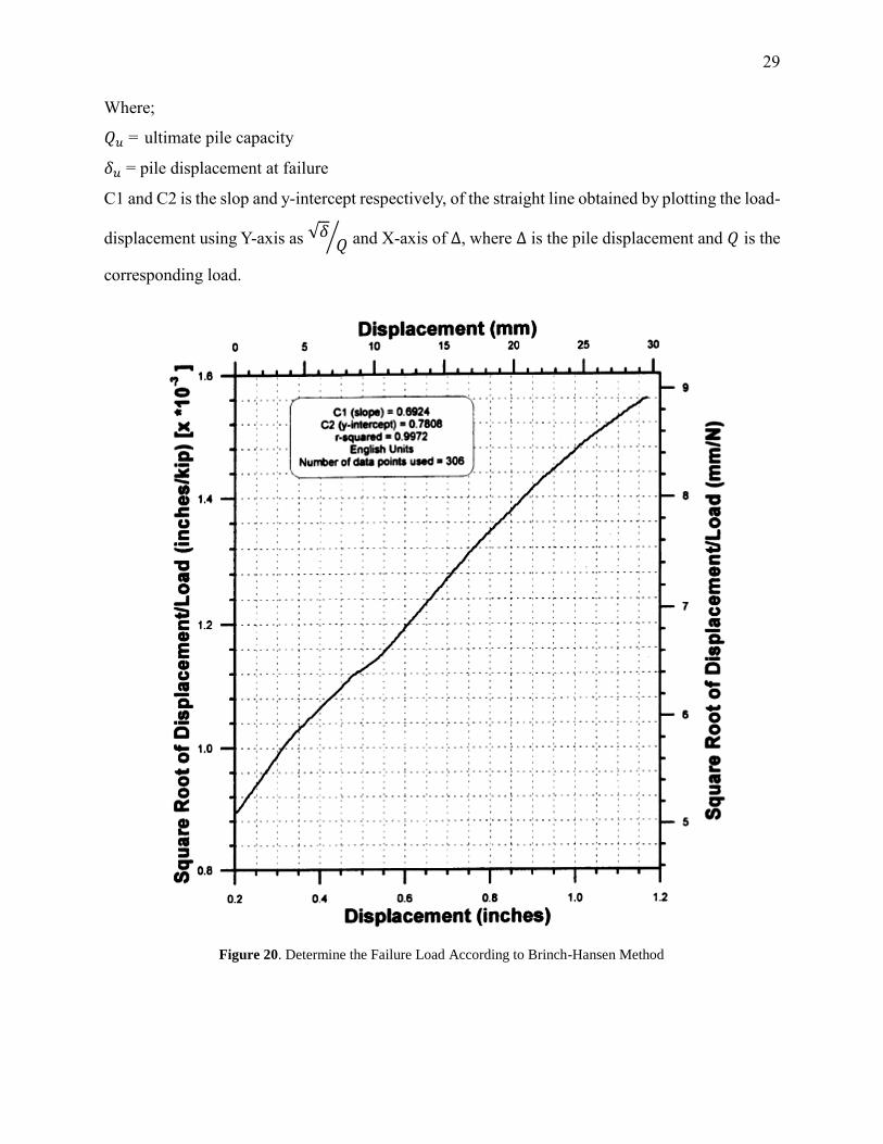
Where;
𝑄𝑢 = ultimate pile capacity
𝛿𝑢 = pile displacement at failure
C1 and C2 is the slop and y-intercept respectively, of the straight line obtained by plotting the load-
displacement using Y-axis as √𝛿𝑄⁄ and X-axis of ∆, where ∆ is the pile displacement and 𝑄 is the
corresponding load.
Figure 20. Determine the Failure Load According to Brinch-Hansen Method
30
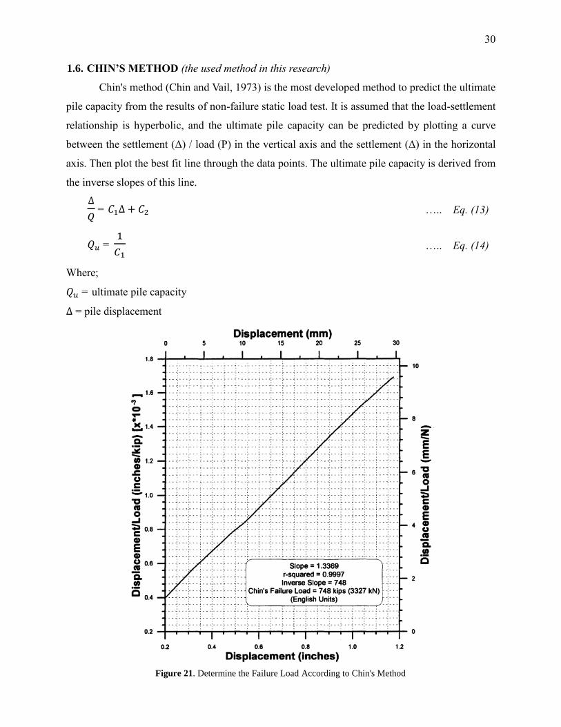
1.6. CHIN’S METHOD (the used method in this research)
Chin's method (Chin and Vail, 1973) is the most developed method to predict the ultimate
pile capacity from the results of non-failure static load test. It is assumed that the load-settlement
relationship is hyperbolic, and the ultimate pile capacity can be predicted by plotting a curve
between the settlement (Δ) / load (P) in the vertical axis and the settlement (Δ) in the horizontal
axis. Then plot the best fit line through the data points. The ultimate pile capacity is derived from
the inverse slopes of this line.
∆
𝑄 = 𝐶1∆ + 𝐶2 ….. Eq. (13)
𝑄𝑢 =
1
𝐶1 ….. Eq. (14)
Where;
𝑄𝑢 = ultimate pile capacity
∆ = pile displacement
Figure 21. Determine the Failure Load According to Chin's Method
31
PREDICTION OF PILE CAPACITY FROM NON-DESTRUCTIVE BI-
DIRECTIONAL STATIC LOAD TEST (BDSLT)
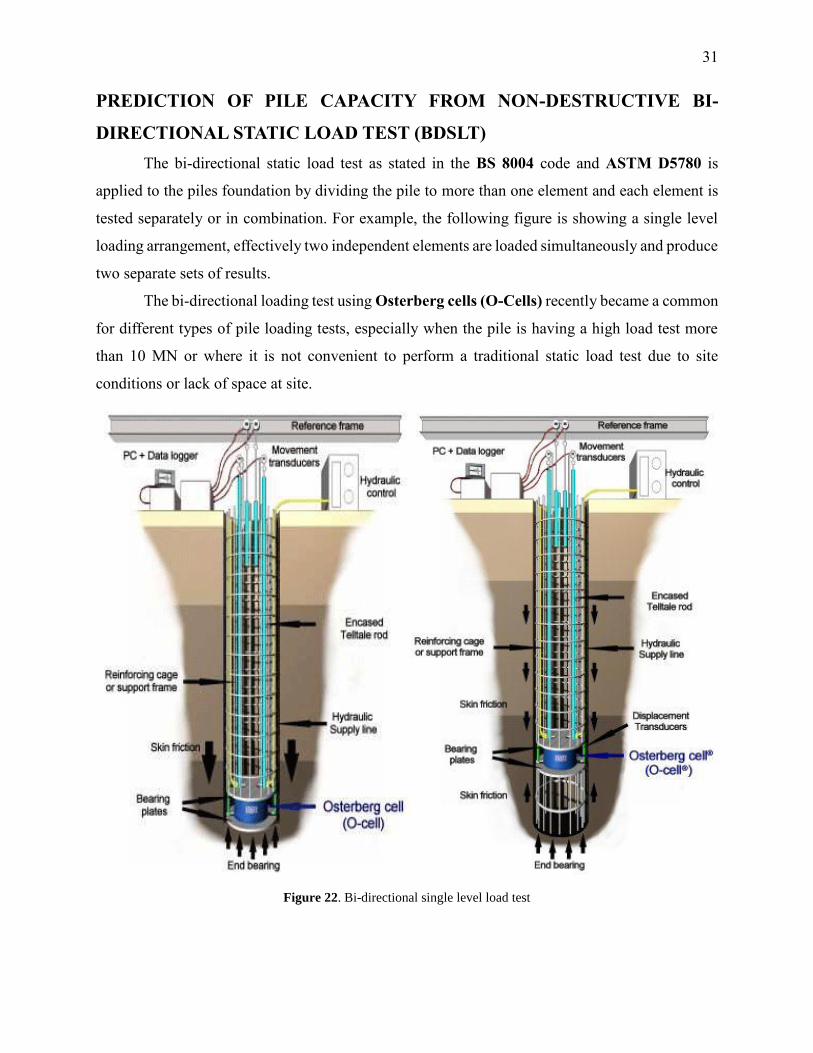
The bi-directional static load test as stated in the BS 8004 code and ASTM D5780 is
applied to the piles foundation by dividing the pile to more than one element and each element is
tested separately or in combination. For example, the following figure is showing a single level
loading arrangement, effectively two independent elements are loaded simultaneously and produce
two separate sets of results.
The bi-directional loading test using Osterberg cells (O-Cells) recently became a common
for different types of pile loading tests, especially when the pile is having a high load test more
than 10 MN or where it is not convenient to perform a traditional static load test due to site
conditions or lack of space at site.
Figure 22. Bi-directional single level load test
32
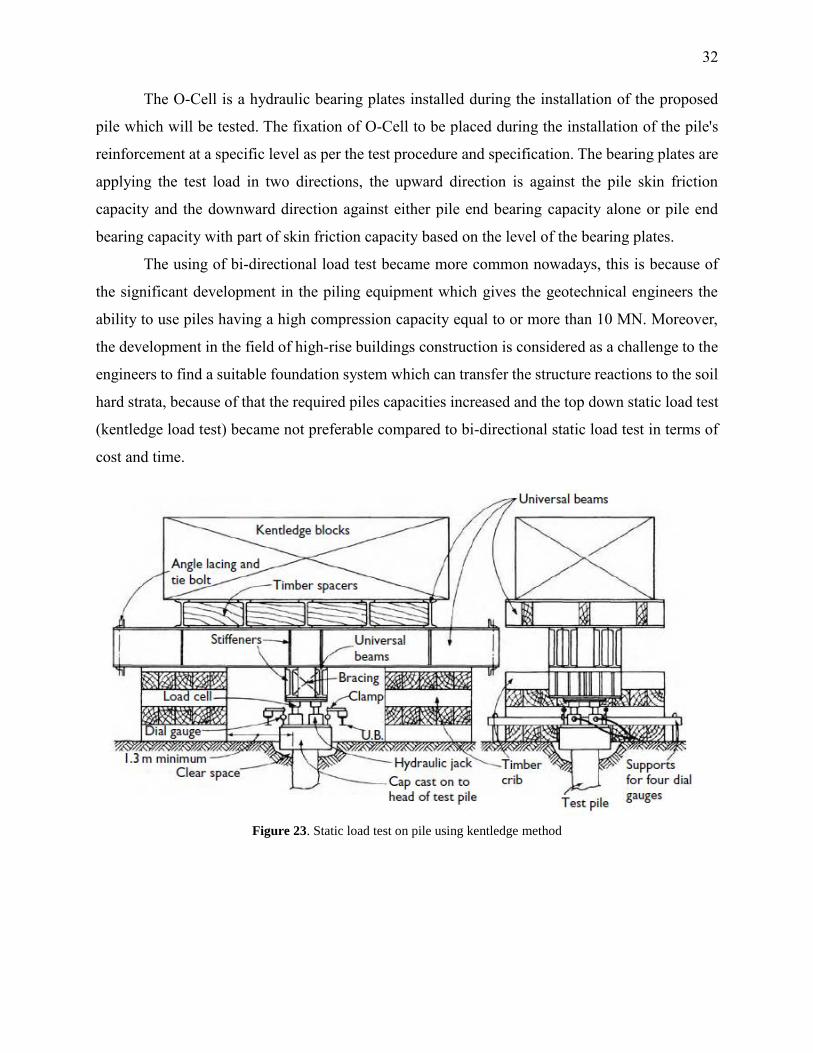
The O-Cell is a hydraulic bearing plates installed during the installation of the proposed
pile which will be tested. The fixation of O-Cell to be placed during the installation of the pile's
reinforcement at a specific level as per the test procedure and specification. The bearing plates are
applying the test load in two directions, the upward direction is against the pile skin friction
capacity and the downward direction against either pile end bearing capacity alone or pile end
bearing capacity with part of skin friction capacity based on the level of the bearing plates.
The using of bi-directional load test became more common nowadays, this is because of
the significant development in the piling equipment which gives the geotechnical engineers the
ability to use piles having a high compression capacity equal to or more than 10 MN. Moreover,
the development in the field of high-rise buildings construction is considered as a challenge to the
engineers to find a suitable foundation system which can transfer the structure reactions to the soil
hard strata, because of that the required piles capacities increased and the top down static load test
(kentledge load test) became not preferable compared to bi-directional static load test in terms of
cost and time.
Figure 23. Static load test on pile using kentledge method
33
The following items show the main differences between the top down static load test
(Kentledge load test) and the bi-directional static load test;
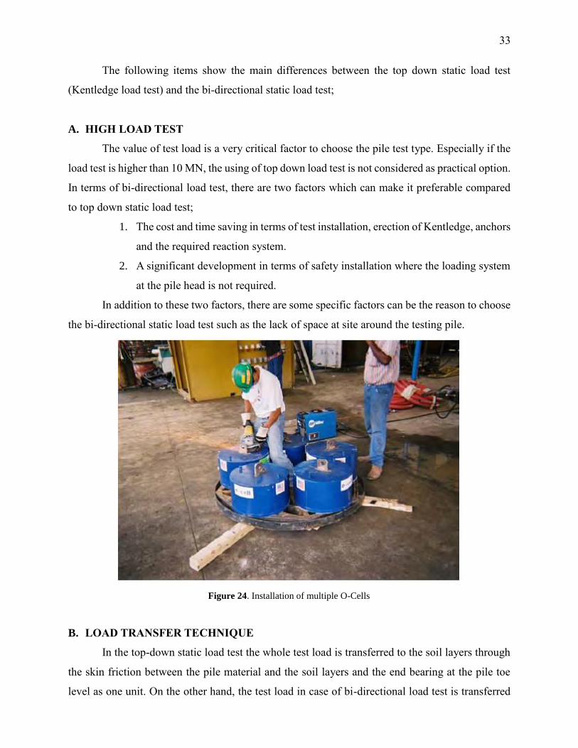
A. HIGH LOAD TEST
The value of test load is a very critical factor to choose the pile test type. Especially if the
load test is higher than 10 MN, the using of top down load test is not considered as practical option.
In terms of bi-directional load test, there are two factors which can make it preferable compared
to top down static load test;
1. The cost and time saving in terms of test installation, erection of Kentledge, anchors
and the required reaction system.
2. A significant development in terms of safety installation where the loading system
at the pile head is not required.
In addition to these two factors, there are some specific factors can be the reason to choose
the bi-directional static load test such as the lack of space at site around the testing pile.
B. LOAD TRANSFER TECHNIQUE
In the top-down static load test the whole test load is transferred to the soil layers through
the skin friction between the pile material and the soil layers and the end bearing at the pile toe
level as one unit. On the other hand, the test load in case of bi-directional load test is transferred
Figure 24. Installation of multiple O-Cells
34
to the soil based on the test arrangement. For example, the single level bi-directional test has two
segments. The upper segment resists the test load by the skin friction between the pile material and
the upper soil layers which are around the upper pile segment. The lower segment resists the test
loading by the end bearing or end bearing with partial skin friction based on the O-Cell level
compared to the pile toe level.
EQUIVALENT TOP-DOWN STATIC LOADED LOAD-SETTLEMENT CURVE FROM
THE RESULTS OF A BI-DIRECTIONAL STATIC LOAD TEST (BDSLT)
The BDSLT is used as alternative solution to the top-down static load test in some specific
cases. But the test results should be analyzed to generate the load versus settlement curve which is
used to understand the pile behavior during the loading test. To estimate the load-settlement curve
from a BDSLT, there are some assumption should be taken into consideration as follows;
1. The upper skin friction (side shear) load-movement curve resulting from the
upward movement of O-Cell is equal to the settlement of the pile head in a
conventional top-down static load test.
2. The part of the pile shaft below the O-Cell has the same load-movement behavior
as the downward pile movement in a conventional top-down static load test. The
subsequent movement curve in the BDSLT refers to the combined lower skin
friction and end bearing movement of the entire length of pile shaft below the O-
Cell level (2nd segment)
3. The pile is considered as rigid body, but the elastic deformation of the pile is
considered in the estimation of the load-settlement curve as a correction procedure.
PROCEDURE A
This procedure complies with the above assumptions, to construct the equivalent load-
settlement curve the following steps should be followed;
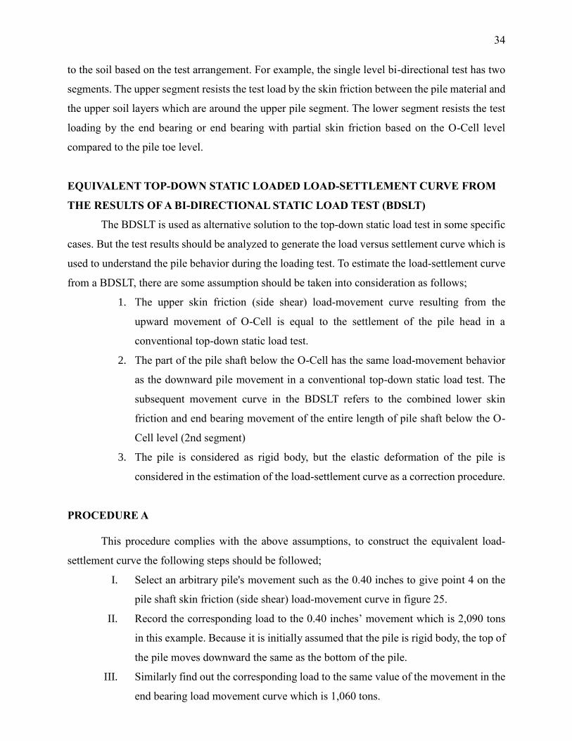
I. Select an arbitrary pile's movement such as the 0.40 inches to give point 4 on the
pile shaft skin friction (side shear) load-movement curve in figure 25.
II. Record the corresponding load to the 0.40 inches’ movement which is 2,090 tons
in this example. Because it is initially assumed that the pile is rigid body, the top of
the pile moves downward the same as the bottom of the pile.
III. Similarly find out the corresponding load to the same value of the movement in the
end bearing load movement curve which is 1,060 tons.
35
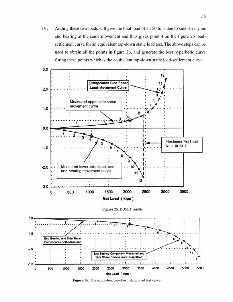
IV. Adding these two loads will give the total load of 3,150 tons due to side shear plus
end bearing at the same movement and thus gives point 4 on the figure 26 load-
settlement curve for an equivalent top-down static load test. The above steps can be
used to obtain all the points in figure 26, and generate the best hyperbolic curve
fitting these points which is the equivalent top-down static load-settlement curve.
Figure 25. BDSLT results
Figure 26. The equivalent top-down static load test curve
36
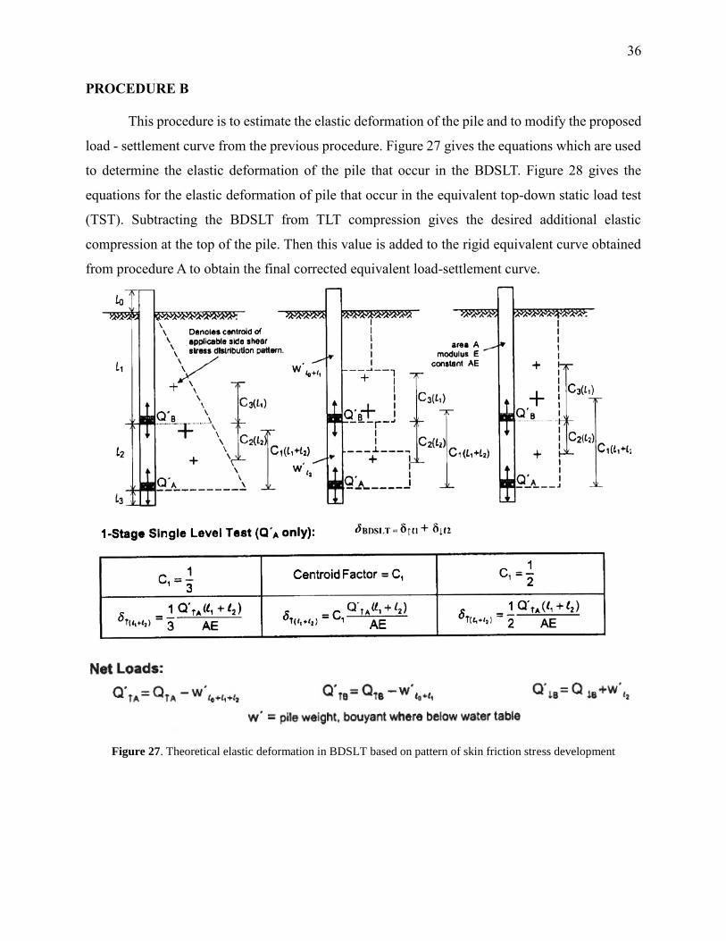
PROCEDURE B
This procedure is to estimate the elastic deformation of the pile and to modify the proposed
load - settlement curve from the previous procedure. Figure 27 gives the equations which are used
to determine the elastic deformation of the pile that occur in the BDSLT. Figure 28 gives the
equations for the elastic deformation of pile that occur in the equivalent top-down static load test
(TST). Subtracting the BDSLT from TLT compression gives the desired additional elastic
compression at the top of the pile. Then this value is added to the rigid equivalent curve obtained
from procedure A to obtain the final corrected equivalent load-settlement curve.
Figure 27. Theoretical elastic deformation in BDSLT based on pattern of skin friction stress development

37
Figure 28. Theoretical elastic deformation in top-down static load test based on pattern of skin friction stress
development
38
LONG / MEGA PILING SYSTEM FOR HIGH-RISE BUILDINGS
In the last two decades there was a significant development in terms of high-rise buildings
construction. The developed countries are competing with each other to build higher buildings
which are used as icon for each country. In consequence, the engineers have been subjected to
different challenges, to achieve the structural stability of the high-rise buildings. One of the major
types of these challenges is the foundation system of high-rise building. The most used foundation
system is the piled raft foundation system, the piles depth in this case can be reach 40 to 60 m
which is considered as long piles. The definition of long piles is these piles which are having a
depth equal to or more than 20 to 25 m. This chapter will discuss some aspect of design and
construction of long bored pile foundation system and brief about the pile's bearing behavior.
INTRODUCTION
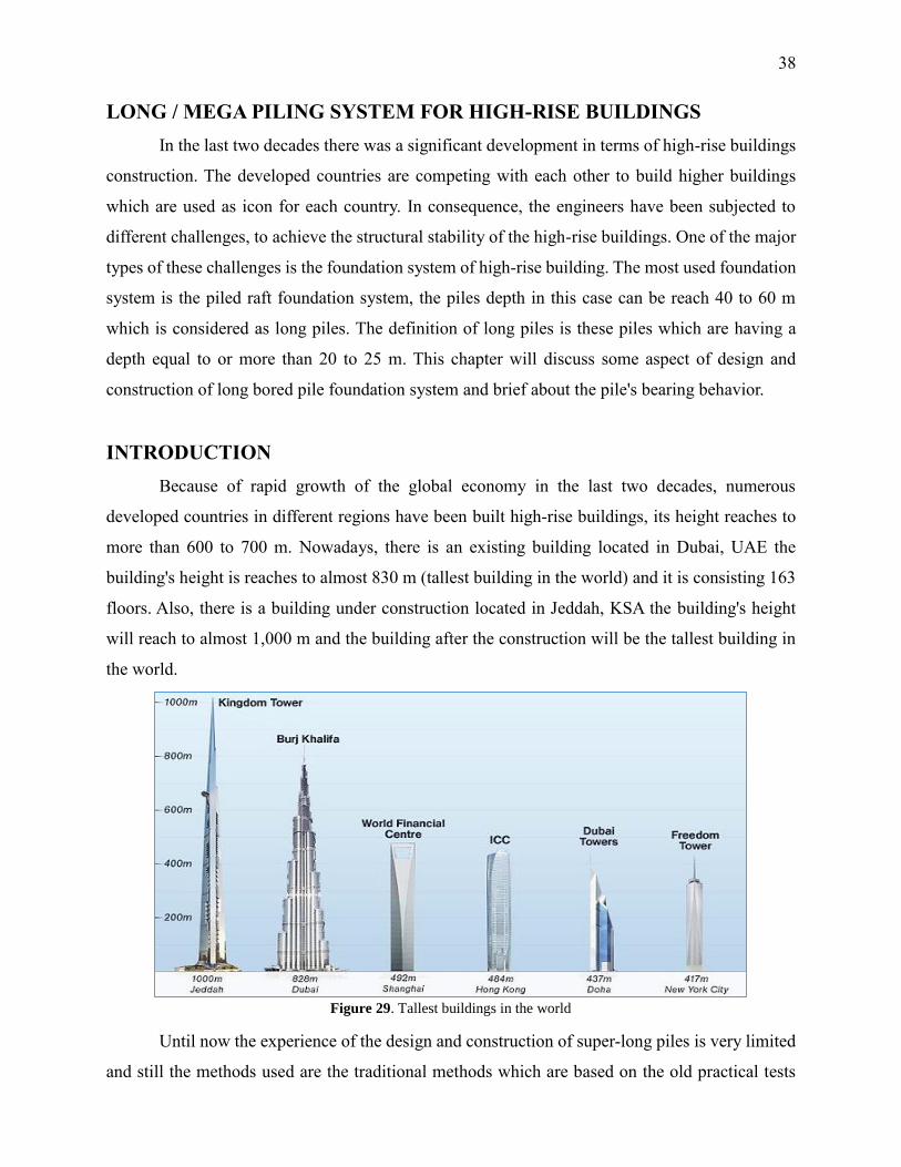
Because of rapid growth of the global economy in the last two decades, numerous
developed countries in different regions have been built high-rise buildings, its height reaches to
more than 600 to 700 m. Nowadays, there is an existing building located in Dubai, UAE the
building's height is reaches to almost 830 m (tallest building in the world) and it is consisting 163
floors. Also, there is a building under construction located in Jeddah, KSA the building's height
will reach to almost 1,000 m and the building after the construction will be the tallest building in
the world.
Until now the experience of the design and construction of super-long piles is very limited
and still the methods used are the traditional methods which are based on the old practical tests
Figure 29. Tallest buildings in the world
39
which have been done on short piles. Therefore, geotechnical engineers are being forced to develop
these traditional design methods to match the current situation of the developed construction
methods and the developed drilling techniques. The following sections in this chapter will give a
simple idea about the super-long piles in terms of construction and design.
BEARING BEHAVIORS OF LONG PILE
Long piles mainly represent the piles with depth larger than 35 m and slenderness ratio
(L/D) larger than 30, Where L is the pile depth and D is the pile diameter. Both theoretical studies
and engineering practices show that the long piles behaviors are different from short piles. This is
because there are many soil layers around the piles shaft, this leads to complex behavior in terms
of pile shaft resistance of long piles compare to short piles. Furthermore, because of the large pile
length and high slenderness ratio of the long bored pile, the stiffness of pile-soil system is relatively
small. This influences the bearing characteristics of the long piles. With reference to the analysis
of practical load tests results (Zhang and Liu, 2009), the basic bearing behaviors of long piles
summarized in the following steps:
1. The pile load - settlement curve has no significant change in the slope, in case of
the pile tip is post grouted.
2. In case of ultimate bearing load, the settlement of the pile head is mainly caused by
pile shaft compression, especially the upper half of pile shaft. In addition, the pile
shaft presents large plastic deformation under high load.
3. The pile shaft friction in the top soil layers is mobilized before that in the deep
layers.
4. The mobilization of the pile shaft friction is dependent on the support condition at
the pile tip. Therefore, the pile tip resistance and pile shaft friction can be increased
significantly in case of the support condition is improved by post grouting at pile
tip.
40
CHAPTER 2 – RESEARCH METHODOLOGY
The main purpose of the research is to compare between the theoretical, practical and
numerical pile compression capacities. The research concentrate on the piles which had been
installed in Dubai. And the research methodology is summarized in the following procedure;
1. Selection of three different cases of study (project) and collection of all required data
which are required to determinate the pile capacities like;
A. Project piling drawing including all the information about the pile such as
pile cutoff level, pile toe level, pile diameter and the demanded pile capacity.
B. Project soil investigation report including all the information about the soil
layers’ classifications and the recommendations about the piles foundation.
C. The results of pile’s static load test results, this is to predict the practical
pile capacity by using Chin’s method (see Section 1.6) in case of non-
destructive static load test.
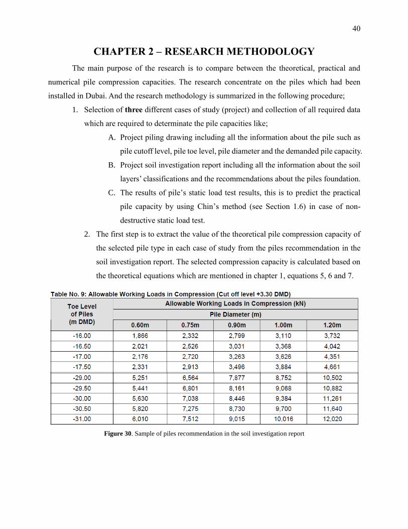
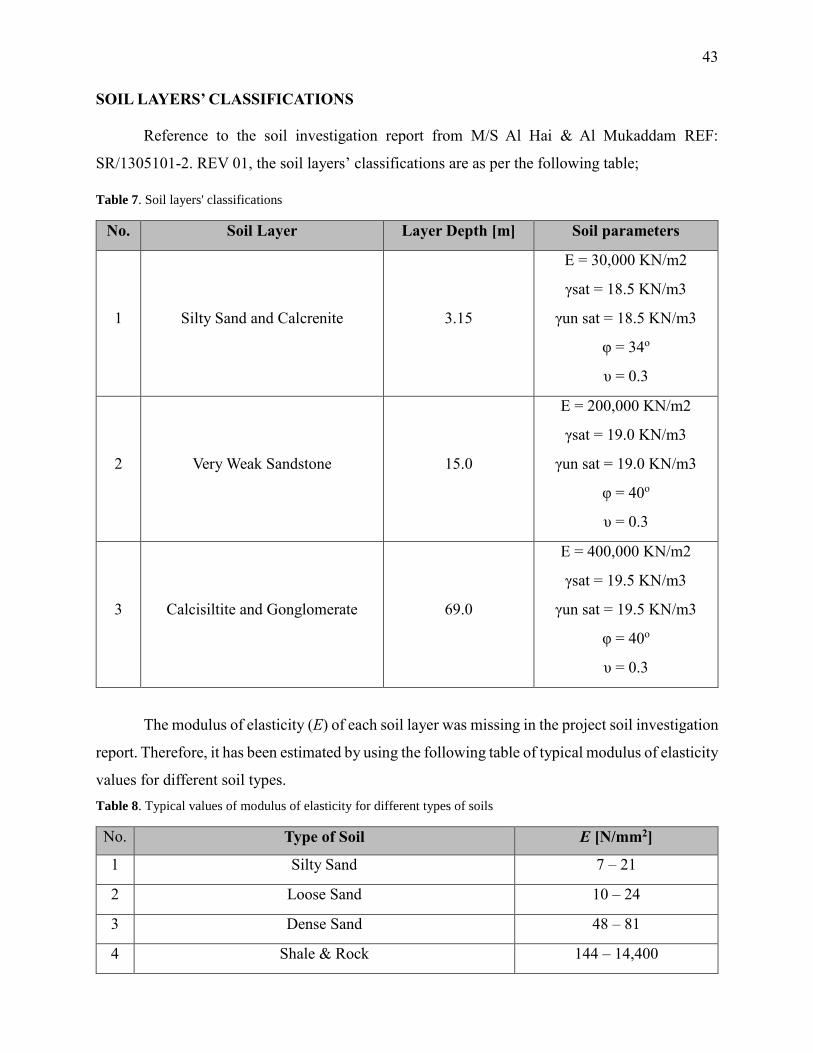
2. The first step is to extract the value of the theoretical pile compression capacity of
the selected pile type in each case of study from the piles recommendation in the
soil investigation report. The selected compression capacity is calculated based on
the theoretical equations which are mentioned in chapter 1, equations 5, 6 and 7.
Figure 30. Sample of piles recommendation in the soil investigation report

41
3. The practical pile capacity of the selected pile from each case of study will be
estimated by using Chin's method (see Section 1.6). Chin's method is the most
developed method to predict the ultimate pile capacity from the results of non-
failure static load test. The used data to plot the Chin's curve are based on the actual
results of pile's static load test by using one of the following techniques the first is
kentledge load test or the second which is the bidirectional static load test.
4. For numerical pile capacity, a finite element model for the selected pile type from
each case will be modeled by using PLAXIS 2D software to get the piles
compression capacity. All the soil parameters which will be used in the numerical
model will be extracted from the soil investigation report of each case.
5. Finally, a Comparison between theoretical, practical and numerical pile capacity of
each case will be done and will be discussed in details.
CASES OF STUDY
Three cases of study have been chosen to be used in this research, this section will cover
each case of study's description and the selected pile details.
CASE 1 _ AL HABTOOR RESIDENCE
Al Habtoor residence project is consisting 40 floors tower and two numbers of 60 floors
towers over a common podium situated on a 25,000 m2 plot. The project is to have one basement
for parking with an additional 3 parking floors within the podium. The ground floor of the podium
includes retail spaces whilst the top of the podium is landscaped with facilities for tenants.
Figure 31. Al Habtoor residence
42
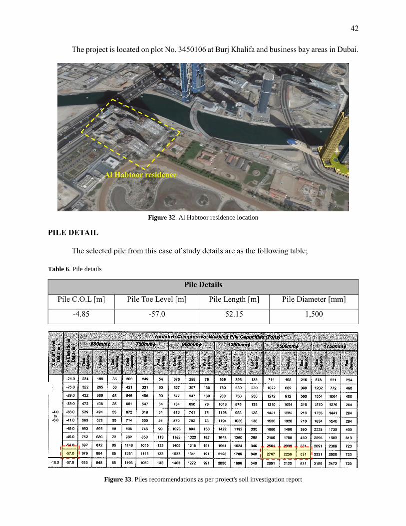
The project is located on plot No. 3450106 at Burj Khalifa and business bay areas in Dubai.
PILE DETAIL
The selected pile from this case of study details are as the following table;
Table 6. Pile details
Pile Details
Pile C.O.L [m] Pile Toe Level [m] Pile Length [m] Pile Diameter [mm]
-4.85 -57.0 52.15 1,500
Figure 32. Al Habtoor residence location
Figure 33. Piles recommendations as per project's soil investigation report
43
SOIL LAYERS’ CLASSIFICATIONS
Reference to the soil investigation report from M/S Al Hai & Al Mukaddam REF:
SR/1305101-2. REV 01, the soil layers’ classifications are as per the following table;
Table 7. Soil layers' classifications
No. Soil Layer Layer Depth [m] Soil parameters
1 Silty Sand and Calcrenite 3.15
E = 30,000 KN/m2
γsat = 18.5 KN/m3
γun sat = 18.5 KN/m3
φ = 34o
υ = 0.3
2 Very Weak Sandstone 15.0
E = 200,000 KN/m2
γsat = 19.0 KN/m3
γun sat = 19.0 KN/m3
φ = 40o
υ = 0.3
3 Calcisiltite and Gonglomerate 69.0
E = 400,000 KN/m2
γsat = 19.5 KN/m3
γun sat = 19.5 KN/m3
φ = 40o
υ = 0.3
The modulus of elasticity (E) of each soil layer was missing in the project soil investigation
report. Therefore, it has been estimated by using the following table of typical modulus of elasticity
values for different soil types.
Table 8. Typical values of modulus of elasticity for different types of soils
No. Type of Soil E [N/mm2]
1 Silty Sand 7 – 21
2 Loose Sand 10 – 24
3 Dense Sand 48 – 81
4 Shale & Rock 144 – 14,400
44
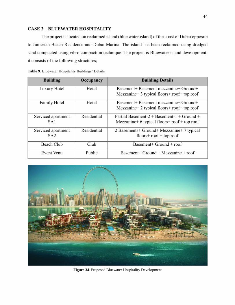
CASE 2 _ BLUEWATER HOSPITALITY
The project is located on reclaimed island (blue water island) of the coast of Dubai opposite
to Jumeriah Beach Residence and Dubai Marina. The island has been reclaimed using dredged
sand compacted using vibro compaction technique. The project is Bluewater island development;
it consists of the following structures;
Table 9. Bluewater Hospitality Buildings’ Details
Building Occupancy Building Details
Luxury Hotel Hotel Basement+ Basement mezzanine+ Ground+
Mezzanine+ 3 typical floors+ roof+ top roof
Family Hotel Hotel Basement+ Basement mezzanine+ Ground+
Mezzanine+ 2 typical floors+ roof+ top roof
Serviced apartment
SA1
Residential Partial Basement-2 + Basement-1 + Ground +
Mezzanine+ 6 typical floors+ roof + top roof
Serviced apartment
SA2
Residential 2 Basements+ Ground+ Mezzanine+ 7 typical
floors+ roof + top roof
Beach Club Club Basement+ Ground + roof
Event Venu Public Basement+ Ground + Mezzanine + roof
Figure 34. Proposed Bluewater Hospitality Development

45
PILE DETAIL
The selected pile from this case of study details are as the following table;
Table 10. Pile Details.
Pile Details
Pile C.O.L [m] Pile Toe Level [m] Pile Length [m] Pile Diameter [mm]
+3.375 DMD -31.0 DMD 34.375 900
Figure 35. Piles recommendations as per project's soil investigation report
46
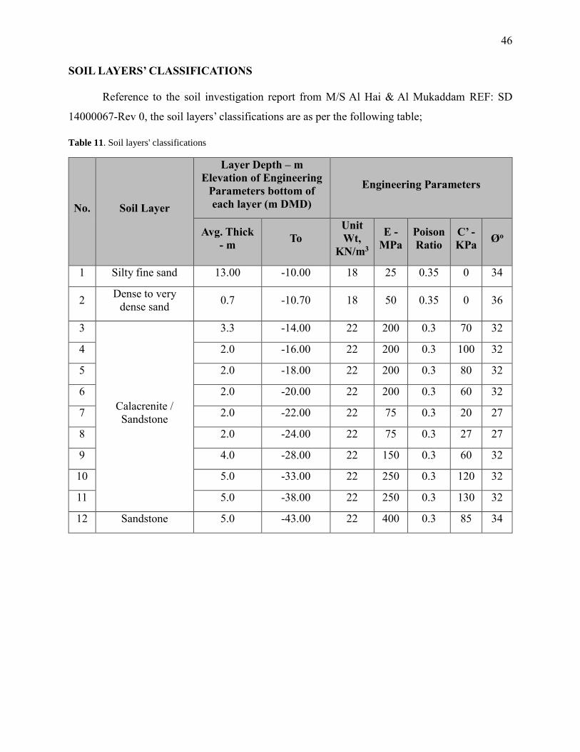
SOIL LAYERS’ CLASSIFICATIONS
Reference to the soil investigation report from M/S Al Hai & Al Mukaddam REF: SD
14000067-Rev 0, the soil layers’ classifications are as per the following table;
Table 11. Soil layers' classifications
No. Soil Layer
Layer Depth – m
Elevation of Engineering
Parameters bottom of
each layer (m DMD)
Engineering Parameters
Avg. Thick
- m To
Unit
Wt,
KN/m3
E -
MPa
Poison
Ratio
C’ -
KPa Øo
1 Silty fine sand 13.00 -10.00 18 25 0.35 0 34
2 Dense to very
dense sand 0.7 -10.70 18 50 0.35 0 36
3
Calacrenite /
Sandstone
3.3 -14.00 22 200 0.3 70 32
4 2.0 -16.00 22 200 0.3 100 32
5 2.0 -18.00 22 200 0.3 80 32
6 2.0 -20.00 22 200 0.3 60 32
7 2.0 -22.00 22 75 0.3 20 27
8 2.0 -24.00 22 75 0.3 27 27
9 4.0 -28.00 22 150 0.3 60 32
10 5.0 -33.00 22 250 0.3 120 32
11 5.0 -38.00 22 250 0.3 130 32
12 Sandstone 5.0 -43.00 22 400 0.3 85 34
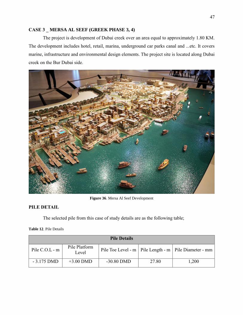
47
CASE 3 _ MERSA AL SEEF (GREEK PHASE 3, 4)
The project is development of Dubai creek over an area equal to approximately 1.80 KM.
The development includes hotel, retail, marina, underground car parks canal and ...etc. It covers
marine, infrastructure and environmental design elements. The project site is located along Dubai
creek on the Bur Dubai side.
PILE DETAIL
The selected pile from this case of study details are as the following table;
Table 12. Pile Details
Pile Details
Pile C.O.L - m Pile Platform
Level Pile Toe Level - m Pile Length - m Pile Diameter - mm
- 3.175 DMD +3.00 DMD -30.80 DMD 27.80 1,200
Figure 36. Mersa Al Seef Development
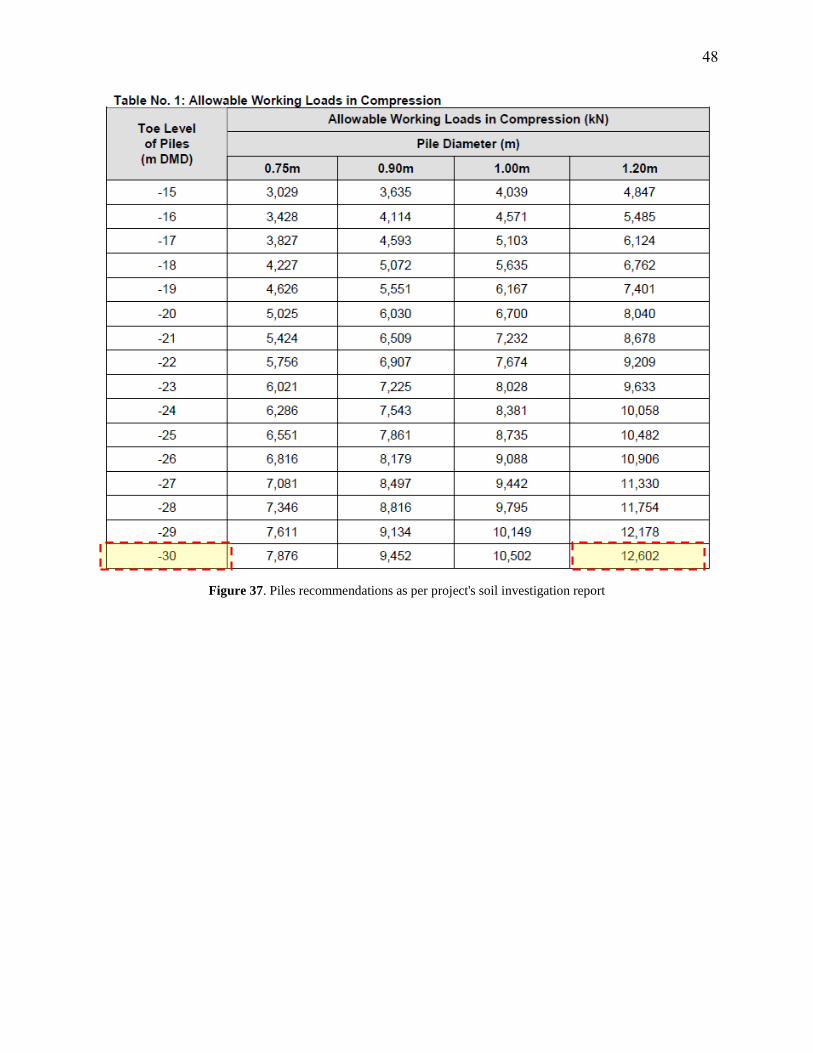
48
Figure 37. Piles recommendations as per project's soil investigation report
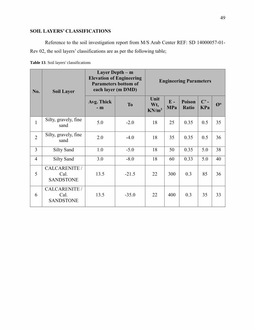
49
SOIL LAYERS’ CLASSIFICATIONS
Reference to the soil investigation report from M/S Arab Center REF: SD 14000057-01-
Rev 02, the soil layers’ classifications are as per the following table;
Table 13. Soil layers' classifications
No. Soil Layer
Layer Depth – m
Elevation of Engineering
Parameters bottom of
each layer (m DMD)
Engineering Parameters
Avg. Thick
- m To
Unit
Wt,
KN/m3
E -
MPa
Poison
Ratio
C’ -
KPa Øo
1 Silty, gravely, fine
sand 5.0 -2.0 18 25 0.35 0.5 35
2 Silty, gravely, fine
sand 2.0 -4.0 18 35 0.35 0.5 36
3 Silty Sand 1.0 -5.0 18 50 0.35 5.0 38
4 Silty Sand 3.0 -8.0 18 60 0.33 5.0 40
5
CALCARENITE /
Cal.
SANDSTONE
13.5 -21.5 22 300 0.3 85 36
6
CALCARENITE /
Cal.
SANDSTONE
13.5 -35.0 22 400 0.3 35 33
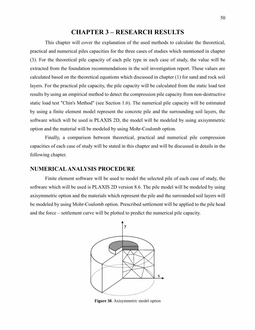
50
CHAPTER 3 – RESEARCH RESULTS
This chapter will cover the explanation of the used methods to calculate the theoretical,
practical and numerical piles capacities for the three cases of studies which mentioned in chapter
(3). For the theoretical pile capacity of each pile type in each case of study, the value will be
extracted from the foundation recommendations in the soil investigation report. These values are
calculated based on the theoretical equations which discussed in chapter (1) for sand and rock soil
layers. For the practical pile capacity, the pile capacity will be calculated from the static load test
results by using an empirical method to detect the compression pile capacity from non-destructive
static load test "Chin's Method" (see Section 1.6). The numerical pile capacity will be estimated
by using a finite element model represent the concrete pile and the surrounding soil layers, the
software which will be used is PLAXIS 2D, the model will be modeled by using axisymmetric
option and the material will be modeled by using Mohr-Coulomb option.
Finally, a comparison between theoretical, practical and numerical pile compression
capacities of each case of study will be stated in this chapter and will be discussed in details in the
following chapter.
NUMERICAL ANALYSIS PROCEDURE
Finite element software will be used to model the selected pile of each case of study, the
software which will be used is PLAXIS 2D version 8.6. The pile model will be modeled by using
axisymmetric option and the materials which represent the pile and the surrounded soil layers will
be modeled by using Mohr-Coulomb option. Prescribed settlement will be applied to the pile head
and the force – settlement curve will be plotted to predict the numerical pile capacity.
Figure 38. Axisymmetric model option

51
The major aspects in the modeling process are the graphical boundaries, soil layers’
classification and parameters and the pile material - soil layers’ friction angle. These factors will
be discussed in details in the following sections;
GRAPHICAL BOUNDARIES
The following figure shows the model's graphical boundaries which should be followed in
the modeling process.
The boundaries are as follows;
D is the pile radius.
Two layers of mesh transition, each layer width is equal to 3D.
L is the pile depth.
The model dimensions are equal to 2.5L for the model depth and 2.0L for the model
width.
The horizontal and vertical displacement of the model edge are not allowed.
Figure 39. Graphical boundaries for the pile model
52
SOIL LAYERS’ CLASSIFICATION AND PARAMETERS
For the soil layers' classifications and the soil parameters which will be used in the
numerical model will be estimated or derived from the soil investigation report of each case of
study. soil layers' modulus of elasticity, cohesion, soil unit weight and the angle of internal friction
of each layer are the major important factors which should be identified and used in the pile model.
PILE - SOIL FRICTION RELATIONSHIP
One of the important factors which has a significant impact on the pile skin friction
resistance is the pile - soil interface condition. This factor depends on the following properties;
A. Soil layers’ classification.
B. Pile material.
C. The installation technique, for example the using of bentonite slurry in the pile
installation has a negative impact on the skin friction resistance compared to the
other techniques like bored pile or CFA technique. This is because the using of
bentonite slurry generates a smooth surface between the pile and the surrounding
soil.
Generally, the reduction factor of skin friction resistance due to interface condition has a
value between 1.0 to 0.5, in this research the used reduction factor for sand soil layers is 0.8 and
the value of the rock soil layers is 0.9 (see Table 2).
CASE 1 _ AL HABTOOR RESIDENCE
A. THEIORTICAL PILE CAPACITY (CASE 1)
Reference to the soil investigation report from M/S Al Hai & Al Mukaddam REF:
SR/1305101-2. REV 01 (see Appendix 2), the compression capacity of the pile with diameter equal
to 1,500 mm and the toe level is -57.0 m from the cut off level - 4.00 to - 6.00 m is 27,670 KN
(refer to Table 6 and Figure 33). This compression capacity is calculated by using set of theoretical
equations which discussed in chapter 1 for sand and rock soil layers.
B. PRACTICAL PILE CAPACITY (CASE 1)
Bi-directional static loading test has been done to the selected pile PTP03 (see Appendix
2), the test has been done by M/S HSSG (piling contractor) and was monitoring by M/S Arab
Center (specialist soil laboratory). The purpose of the bi-directional static loading test on
instrumented pile was to evaluate the following criteria;
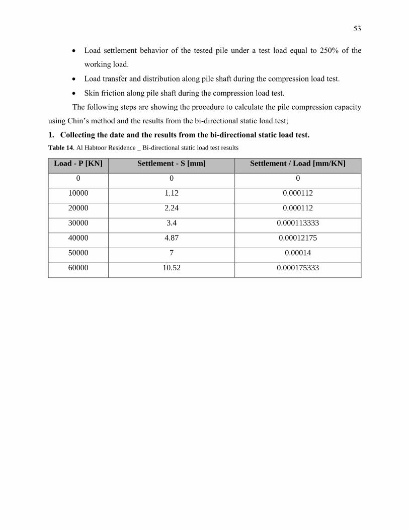
53
Load settlement behavior of the tested pile under a test load equal to 250% of the
working load.
Load transfer and distribution along pile shaft during the compression load test.
Skin friction along pile shaft during the compression load test.
The following steps are showing the procedure to calculate the pile compression capacity
using Chin’s method and the results from the bi-directional static load test;
1. Collecting the date and the results from the bi-directional static load test.
Table 14. Al Habtoor Residence _ Bi-directional static load test results
Load - P [KN] Settlement - S [mm] Settlement / Load [mm/KN]
0 0 0
10000 1.12 0.000112
20000 2.24 0.000112
30000 3.4 0.000113333
40000 4.87 0.00012175
50000 7 0.00014
60000 10.52 0.000175333
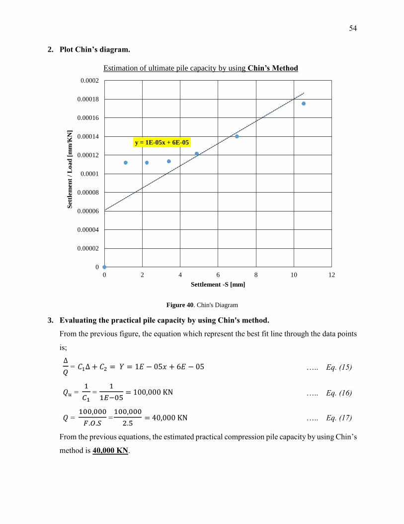
54
2. Plot Chin’s diagram.
Figure 40. Chin's Diagram
3. Evaluating the practical pile capacity by using Chin's method.
From the previous figure, the equation which represent the best fit line through the data points
is;
∆
𝑄 = 𝐶1∆ + 𝐶2 = 𝑌 = 1𝐸 − 05𝑥 + 6𝐸 − 05 ….. Eq. (15)
𝑄𝑢 =
1
𝐶1 =
1
1𝐸−05 = 100,000 KN ….. Eq. (16)
𝑄 =
100,000
𝐹.𝑂.𝑆 =
100,000
2.5 = 40,000 KN ….. Eq. (17)
From the previous equations, the estimated practical compression pile capacity by using Chin’s
method is 40,000 KN.
y = 1E-05x + 6E-05
0
0.00002
0.00004
0.00006
0.00008
0.0001
0.00012
0.00014
0.00016
0.00018
0.0002
0 2 4 6 8 10 12
Set
tlem
ent
/ L
oa
d [
mm
/KN
]
Settlement -S [mm]
Estimation of ultimate pile capacity by using Chin’s Method
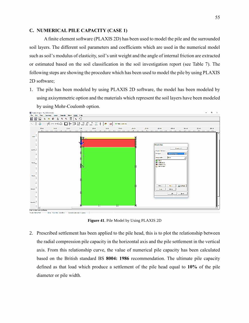
55
C. NUMERICAL PILE CAPACITY (CASE 1)
A finite element software (PLAXIS 2D) has been used to model the pile and the surrounded
soil layers. The different soil parameters and coefficients which are used in the numerical model
such as soil’s modulus of elasticity, soil’s unit weight and the angle of internal friction are extracted
or estimated based on the soil classification in the soil investigation report (see Table 7). The
following steps are showing the procedure which has been used to model the pile by using PLAXIS
2D software;
1. The pile has been modeled by using PLAXIS 2D software, the model has been modeled by
using axisymmetric option and the materials which represent the soil layers have been modeled
by using Mohr-Coulomb option.
2. Prescribed settlement has been applied to the pile head, this is to plot the relationship between
the radial compression pile capacity in the horizontal axis and the pile settlement in the vertical
axis. From this relationship curve, the value of numerical pile capacity has been calculated
based on the British standard BS 8004: 1986 recommendation. The ultimate pile capacity
defined as that load which produce a settlement of the pile head equal to 10% of the pile
diameter or pile width.
Figure 41. Pile Model by Using PLAXIS 2D
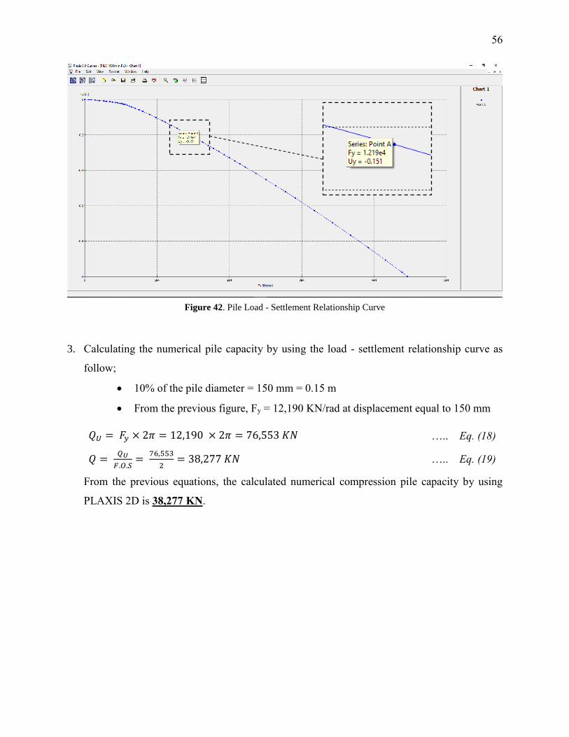
56
3. Calculating the numerical pile capacity by using the load - settlement relationship curve as
follow;
10% of the pile diameter = 150 mm = 0.15 m
From the previous figure, Fy = 12,190 KN/rad at displacement equal to 150 mm
𝑄𝑈 = 𝐹𝑦 × 2𝜋 = 12,190 × 2𝜋 = 76,553 𝐾𝑁 ….. Eq. (18)
𝑄 = 𝑄𝑈
𝐹.𝑂.𝑆=
76,553
2= 38,277 𝐾𝑁 ….. Eq. (19)
From the previous equations, the calculated numerical compression pile capacity by using
PLAXIS 2D is 38,277 KN.
Figure 42. Pile Load - Settlement Relationship Curve
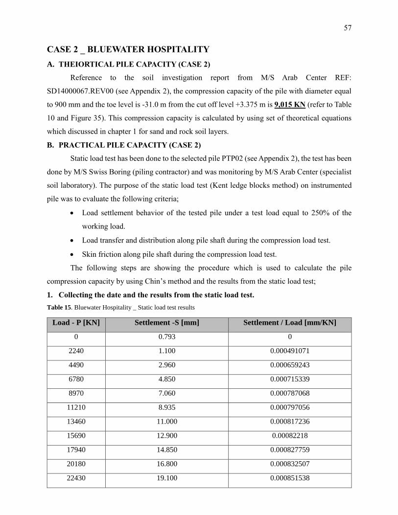
57
CASE 2 _ BLUEWATER HOSPITALITY
A. THEIORTICAL PILE CAPACITY (CASE 2)
Reference to the soil investigation report from M/S Arab Center REF:
SD14000067.REV00 (see Appendix 2), the compression capacity of the pile with diameter equal
to 900 mm and the toe level is -31.0 m from the cut off level +3.375 m is 9,015 KN (refer to Table
10 and Figure 35). This compression capacity is calculated by using set of theoretical equations
which discussed in chapter 1 for sand and rock soil layers.
B. PRACTICAL PILE CAPACITY (CASE 2)
Static load test has been done to the selected pile PTP02 (see Appendix 2), the test has been
done by M/S Swiss Boring (piling contractor) and was monitoring by M/S Arab Center (specialist
soil laboratory). The purpose of the static load test (Kent ledge blocks method) on instrumented
pile was to evaluate the following criteria;
Load settlement behavior of the tested pile under a test load equal to 250% of the
working load.
Load transfer and distribution along pile shaft during the compression load test.
Skin friction along pile shaft during the compression load test.
The following steps are showing the procedure which is used to calculate the pile
compression capacity by using Chin’s method and the results from the static load test;
1. Collecting the date and the results from the static load test.
Table 15. Bluewater Hospitality _ Static load test results
Load - P [KN] Settlement -S [mm] Settlement / Load [mm/KN]
0 0.793 0
2240 1.100 0.000491071
4490 2.960 0.000659243
6780 4.850 0.000715339
8970 7.060 0.000787068
11210 8.935 0.000797056
13460 11.000 0.000817236
15690 12.900 0.00082218
17940 14.850 0.000827759
20180 16.800 0.000832507
22430 19.100 0.000851538
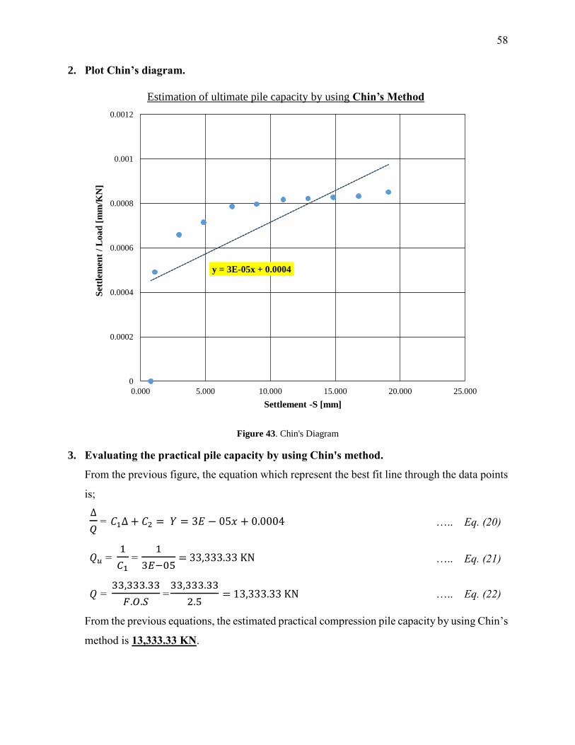
58
2. Plot Chin’s diagram.
Figure 43. Chin's Diagram
3. Evaluating the practical pile capacity by using Chin's method.
From the previous figure, the equation which represent the best fit line through the data points
is;
∆
𝑄 = 𝐶1∆ + 𝐶2 = 𝑌 = 3𝐸 − 05𝑥 + 0.0004 ….. Eq. (20)
𝑄𝑢 =
1
𝐶1 =
1
3𝐸−05 = 33,333.33 KN ….. Eq. (21)
𝑄 =
33,333.33
𝐹.𝑂.𝑆 =
33,333.33
2.5 = 13,333.33 KN ….. Eq. (22)
From the previous equations, the estimated practical compression pile capacity by using Chin’s
method is 13,333.33 KN.
y = 3E-05x + 0.0004
0
0.0002
0.0004
0.0006
0.0008
0.001
0.0012
0.000 5.000 10.000 15.000 20.000 25.000
Set
tlem
ent
/ L
oa
d [
mm
/KN
]
Settlement -S [mm]
Estimation of ultimate pile capacity by using Chin’s Method
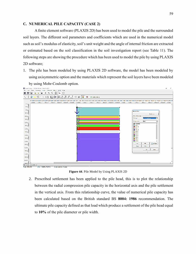
59
C. NUMERICAL PILE CAPACITY (CASE 2)
A finite element software (PLAXIS 2D) has been used to model the pile and the surrounded
soil layers. The different soil parameters and coefficients which are used in the numerical model
such as soil’s modulus of elasticity, soil’s unit weight and the angle of internal friction are extracted
or estimated based on the soil classification in the soil investigation report (see Table 11). The
following steps are showing the procedure which has been used to model the pile by using PLAXIS
2D software;
1. The pile has been modeled by using PLAXIS 2D software, the model has been modeled by
using axisymmetric option and the materials which represent the soil layers have been modeled
by using Mohr-Coulomb option.
2. Prescribed settlement has been applied to the pile head, this is to plot the relationship
between the radial compression pile capacity in the horizontal axis and the pile settlement
in the vertical axis. From this relationship curve, the value of numerical pile capacity has
been calculated based on the British standard BS 8004: 1986 recommendation. The
ultimate pile capacity defined as that load which produce a settlement of the pile head equal
to 10% of the pile diameter or pile width.
Figure 44. Pile Model by Using PLAXIS 2D
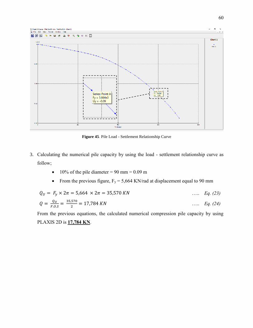
60
3. Calculating the numerical pile capacity by using the load - settlement relationship curve as
follow;
10% of the pile diameter = 90 mm = 0.09 m
From the previous figure, Fy = 5,664 KN/rad at displacement equal to 90 mm
𝑄𝑈 = 𝐹𝑦 × 2𝜋 = 5,664 × 2𝜋 = 35,570 𝐾𝑁 ….. Eq. (23)
𝑄 = 𝑄𝑈
𝐹.𝑂.𝑆=
35,570
2= 17,784 𝐾𝑁 ….. Eq. (24)
From the previous equations, the calculated numerical compression pile capacity by using
PLAXIS 2D is 17,784 KN.
Figure 45. Pile Load - Settlement Relationship Curve
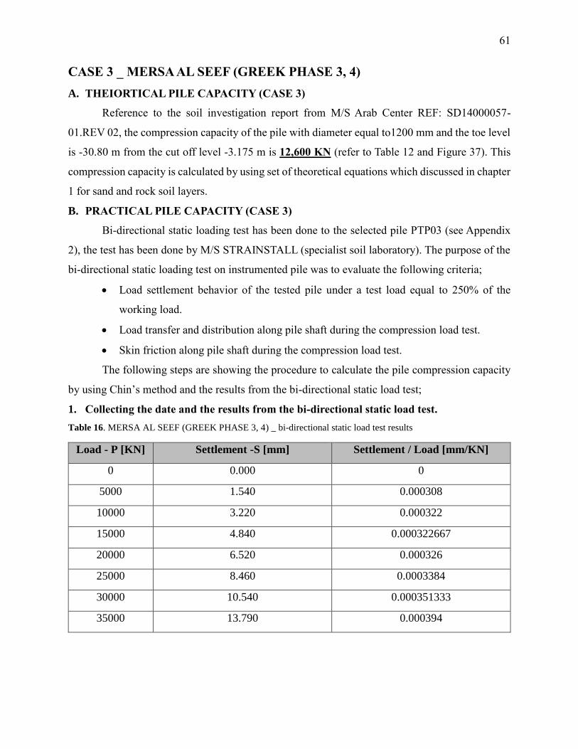
61
CASE 3 _ MERSA AL SEEF (GREEK PHASE 3, 4)
A. THEIORTICAL PILE CAPACITY (CASE 3)
Reference to the soil investigation report from M/S Arab Center REF: SD14000057-
01.REV 02, the compression capacity of the pile with diameter equal to1200 mm and the toe level
is -30.80 m from the cut off level -3.175 m is 12,600 KN (refer to Table 12 and Figure 37). This
compression capacity is calculated by using set of theoretical equations which discussed in chapter
1 for sand and rock soil layers.
B. PRACTICAL PILE CAPACITY (CASE 3)
Bi-directional static loading test has been done to the selected pile PTP03 (see Appendix
2), the test has been done by M/S STRAINSTALL (specialist soil laboratory). The purpose of the
bi-directional static loading test on instrumented pile was to evaluate the following criteria;
Load settlement behavior of the tested pile under a test load equal to 250% of the
working load.
Load transfer and distribution along pile shaft during the compression load test.
Skin friction along pile shaft during the compression load test.
The following steps are showing the procedure to calculate the pile compression capacity
by using Chin’s method and the results from the bi-directional static load test;
1. Collecting the date and the results from the bi-directional static load test.
Table 16. MERSA AL SEEF (GREEK PHASE 3, 4) _ bi-directional static load test results
Load - P [KN] Settlement -S [mm] Settlement / Load [mm/KN]
0 0.000 0
5000 1.540 0.000308
10000 3.220 0.000322
15000 4.840 0.000322667
20000 6.520 0.000326
25000 8.460 0.0003384
30000 10.540 0.000351333
35000 13.790 0.000394
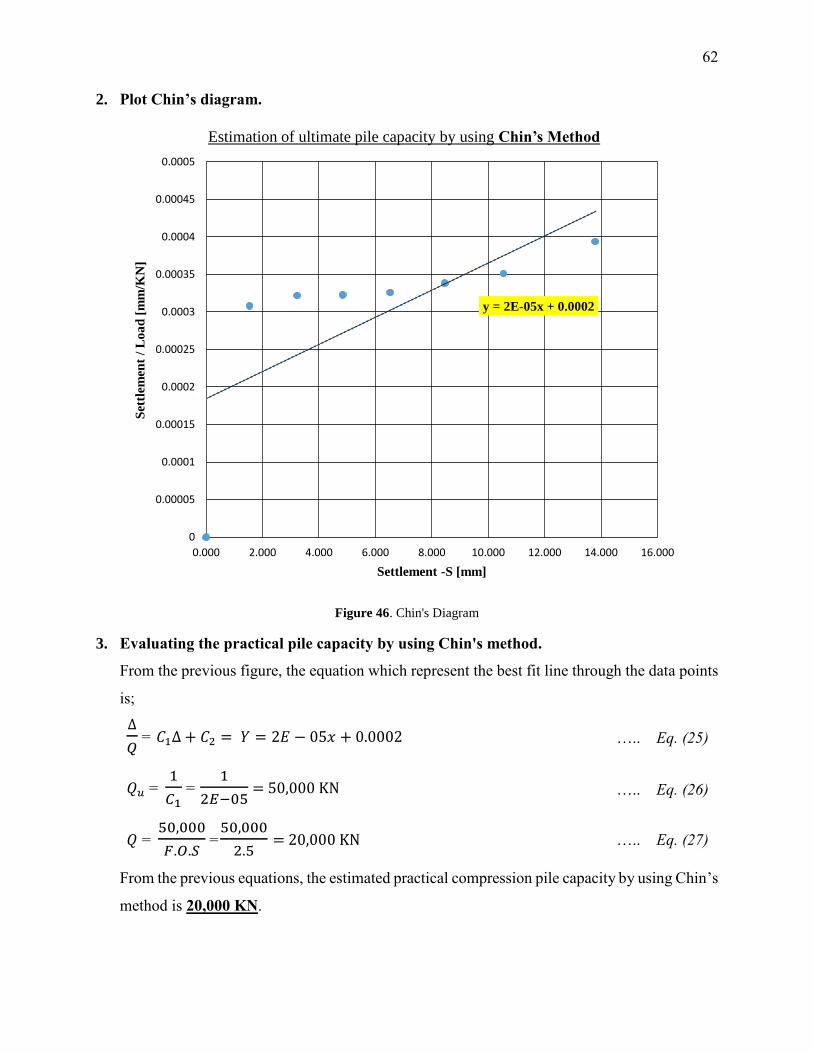
62
2. Plot Chin’s diagram.
Figure 46. Chin's Diagram
3. Evaluating the practical pile capacity by using Chin's method.
From the previous figure, the equation which represent the best fit line through the data points
is;
∆
𝑄 = 𝐶1∆ + 𝐶2 = 𝑌 = 2𝐸 − 05𝑥 + 0.0002 ….. Eq. (25)
𝑄𝑢 =
1
𝐶1 =
1
2𝐸−05 = 50,000 KN ….. Eq. (26)
𝑄 =
50,000
𝐹.𝑂.𝑆 =
50,000
2.5 = 20,000 KN ….. Eq. (27)
From the previous equations, the estimated practical compression pile capacity by using Chin’s
method is 20,000 KN.
y = 2E-05x + 0.0002
0
0.00005
0.0001
0.00015
0.0002
0.00025
0.0003
0.00035
0.0004
0.00045
0.0005
0.000 2.000 4.000 6.000 8.000 10.000 12.000 14.000 16.000
Set
tlem
ent
/ L
oa
d [
mm
/KN
]
Settlement -S [mm]
Estimation of ultimate pile capacity by using Chin’s Method
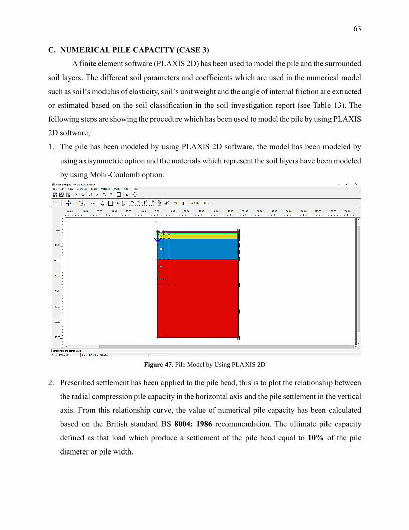
63
C. NUMERICAL PILE CAPACITY (CASE 3)
A finite element software (PLAXIS 2D) has been used to model the pile and the surrounded
soil layers. The different soil parameters and coefficients which are used in the numerical model
such as soil’s modulus of elasticity, soil’s unit weight and the angle of internal friction are extracted
or estimated based on the soil classification in the soil investigation report (see Table 13). The
following steps are showing the procedure which has been used to model the pile by using PLAXIS
2D software;
1. The pile has been modeled by using PLAXIS 2D software, the model has been modeled by
using axisymmetric option and the materials which represent the soil layers have been modeled
by using Mohr-Coulomb option.
2. Prescribed settlement has been applied to the pile head, this is to plot the relationship between
the radial compression pile capacity in the horizontal axis and the pile settlement in the vertical
axis. From this relationship curve, the value of numerical pile capacity has been calculated
based on the British standard BS 8004: 1986 recommendation. The ultimate pile capacity
defined as that load which produce a settlement of the pile head equal to 10% of the pile
diameter or pile width.
Figure 47. Pile Model by Using PLAXIS 2D
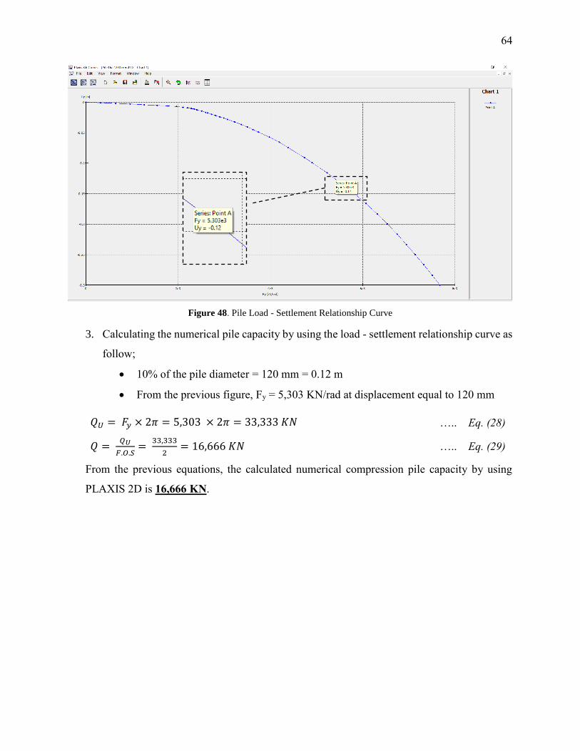
64
3. Calculating the numerical pile capacity by using the load - settlement relationship curve as
follow;
10% of the pile diameter = 120 mm = 0.12 m
From the previous figure, Fy = 5,303 KN/rad at displacement equal to 120 mm
𝑄𝑈 = 𝐹𝑦 × 2𝜋 = 5,303 × 2𝜋 = 33,333 𝐾𝑁 ….. Eq. (28)
𝑄 = 𝑄𝑈
𝐹.𝑂.𝑆=
33,333
2= 16,666 𝐾𝑁 ….. Eq. (29)
From the previous equations, the calculated numerical compression pile capacity by using
PLAXIS 2D is 16,666 KN.
Figure 48. Pile Load - Settlement Relationship Curve
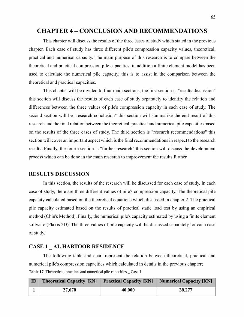
65
CHAPTER 4 – CONCLUSION AND RECOMMENDATIONS
This chapter will discuss the results of the three cases of study which stated in the previous
chapter. Each case of study has three different pile's compression capacity values, theoretical,
practical and numerical capacity. The main purpose of this research is to compare between the
theoretical and practical compression pile capacities, in addition a finite element model has been
used to calculate the numerical pile capacity, this is to assist in the comparison between the
theoretical and practical capacities.
This chapter will be divided to four main sections, the first section is "results discussion"
this section will discuss the results of each case of study separately to identify the relation and
differences between the three values of pile's compression capacity in each case of study. The
second section will be "research conclusion" this section will summarize the end result of this
research and the final relation between the theoretical, practical and numerical pile capacities based
on the results of the three cases of study. The third section is "research recommendations" this
section will cover an important aspect which is the final recommendations in respect to the research
results. Finally, the fourth section is "further research" this section will discuss the development
process which can be done in the main research to improvement the results further.
RESULTS DISCUSSION
In this section, the results of the research will be discussed for each case of study. In each
case of study, there are three different values of pile's compression capacity. The theoretical pile
capacity calculated based on the theoretical equations which discussed in chapter 2. The practical
pile capacity estimated based on the results of practical static load test by using an empirical
method (Chin's Method). Finally, the numerical pile's capacity estimated by using a finite element
software (Plaxis 2D). The three values of pile capacity will be discussed separately for each case
of study.
CASE 1 _ AL HABTOOR RESIDENCE
The following table and chart represent the relation between theoretical, practical and
numerical pile's compression capacities which calculated in details in the previous chapter;
Table 17. Theoretical, practical and numerical pile capacities _ Case 1
ID Theoretical Capacity [KN] Practical Capacity [KN] Numerical Capacity [KN]
1 27,670 40,000 38,277
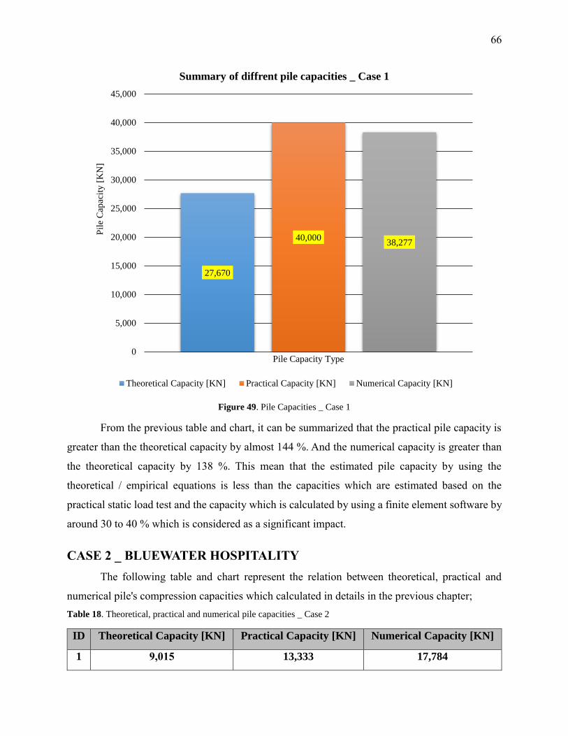
66
From the previous table and chart, it can be summarized that the practical pile capacity is
greater than the theoretical capacity by almost 144 %. And the numerical capacity is greater than
the theoretical capacity by 138 %. This mean that the estimated pile capacity by using the
theoretical / empirical equations is less than the capacities which are estimated based on the
practical static load test and the capacity which is calculated by using a finite element software by
around 30 to 40 % which is considered as a significant impact.
CASE 2 _ BLUEWATER HOSPITALITY
The following table and chart represent the relation between theoretical, practical and
numerical pile's compression capacities which calculated in details in the previous chapter;
Table 18. Theoretical, practical and numerical pile capacities _ Case 2
ID Theoretical Capacity [KN] Practical Capacity [KN] Numerical Capacity [KN]
1 9,015 13,333 17,784
27,670
40,00038,277
0
5,000
10,000
15,000
20,000
25,000
30,000
35,000
40,000
45,000P
ile
Cap
acit
y [
KN
]
Pile Capacity Type
Summary of diffrent pile capacities _ Case 1
Theoretical Capacity [KN] Practical Capacity [KN] Numerical Capacity [KN]
Figure 49. Pile Capacities _ Case 1
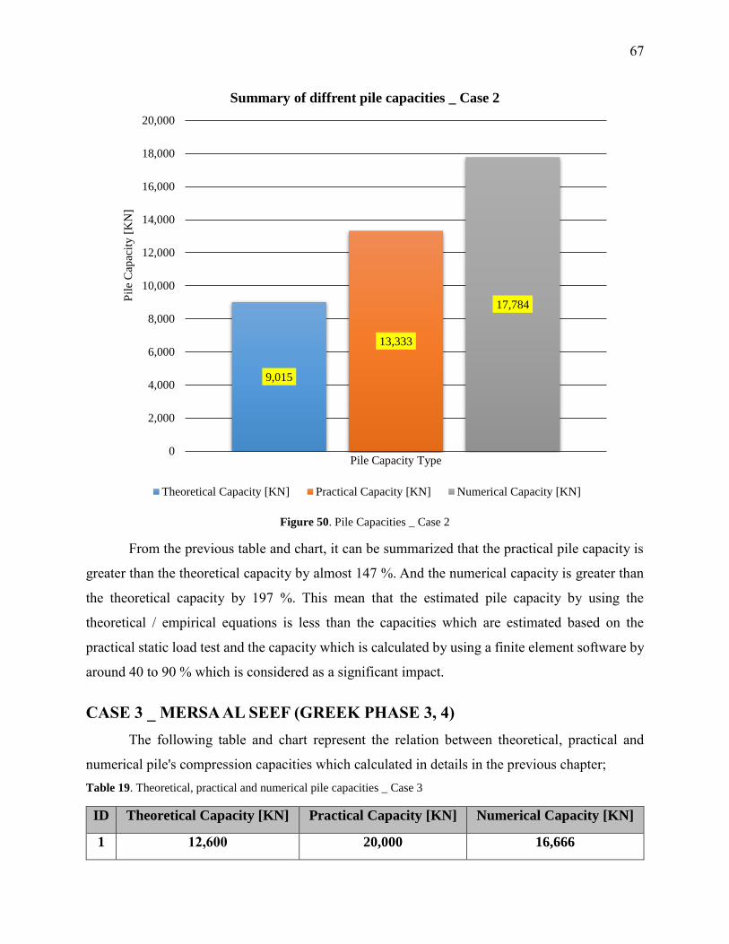
67
From the previous table and chart, it can be summarized that the practical pile capacity is
greater than the theoretical capacity by almost 147 %. And the numerical capacity is greater than
the theoretical capacity by 197 %. This mean that the estimated pile capacity by using the
theoretical / empirical equations is less than the capacities which are estimated based on the
practical static load test and the capacity which is calculated by using a finite element software by
around 40 to 90 % which is considered as a significant impact.
CASE 3 _ MERSA AL SEEF (GREEK PHASE 3, 4)
The following table and chart represent the relation between theoretical, practical and
numerical pile's compression capacities which calculated in details in the previous chapter;
Table 19. Theoretical, practical and numerical pile capacities _ Case 3
ID Theoretical Capacity [KN] Practical Capacity [KN] Numerical Capacity [KN]
1 12,600 20,000 16,666
9,015
13,333
17,784
0
2,000
4,000
6,000
8,000
10,000
12,000
14,000
16,000
18,000
20,000P
ile
Cap
acit
y [
KN
]
Pile Capacity Type
Summary of diffrent pile capacities _ Case 2
Theoretical Capacity [KN] Practical Capacity [KN] Numerical Capacity [KN]
Figure 50. Pile Capacities _ Case 2
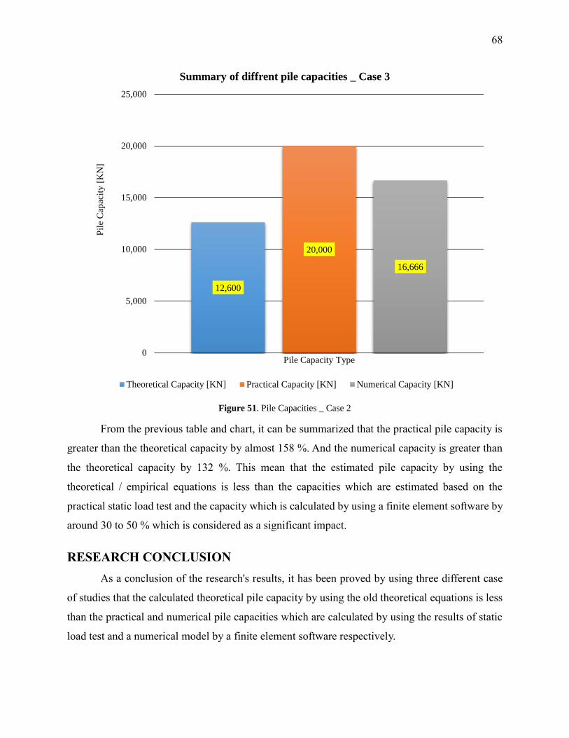
68
From the previous table and chart, it can be summarized that the practical pile capacity is
greater than the theoretical capacity by almost 158 %. And the numerical capacity is greater than
the theoretical capacity by 132 %. This mean that the estimated pile capacity by using the
theoretical / empirical equations is less than the capacities which are estimated based on the
practical static load test and the capacity which is calculated by using a finite element software by
around 30 to 50 % which is considered as a significant impact.
RESEARCH CONCLUSION
As a conclusion of the research's results, it has been proved by using three different case
of studies that the calculated theoretical pile capacity by using the old theoretical equations is less
than the practical and numerical pile capacities which are calculated by using the results of static
load test and a numerical model by a finite element software respectively.
12,600
20,000
16,666
0
5,000
10,000
15,000
20,000
25,000P
ile
Cap
acit
y [
KN
]
Pile Capacity Type
Summary of diffrent pile capacities _ Case 3
Theoretical Capacity [KN] Practical Capacity [KN] Numerical Capacity [KN]
Figure 51. Pile Capacities _ Case 2

69
It has been concluded from case 1 that the practical pile capacity is equal to 144% of the
theoretical pile capacity and the numerical pile capacity is equal to 138% of the theoretical pile
capacity. For case 2, the practical pile capacity is equal to 147% of the theoretical pile capacity
and the numerical pile capacity is equal to 197% of the theoretical pile capacity. Same results in
case 3 where the practical pile capacity is equal to 158% of the theoretical pile capacity and the
numerical pile capacity is equal to 132% of the theoretical pile capacity.
Table 20. Research results
ID Theoretical Capacity
[KN]
Practical Capacity
[KN]
Numerical
Capacity
[KN]
%
(Practical /
Theoretical)
%
(Numerical /
Theoretical)
Case 1 27,670 40,000 38,277 144% 138%
Case 2 9,015 13,333 17,784 147% 197%
Case 3 12,600 20,000 16,666 158% 132%
27,670
9,01512,600
40,000
13,333
20,000
38,277
17,784 16,666
0
5,000
10,000
15,000
20,000
25,000
30,000
35,000
40,000
45,000P
ile
Cap
acit
y [
KN
]
Pile Capacity Type
Research Results
Theoretical Capacity [KN] Practical Capacity [KN] Numerical Capacity [KN]
Case [1] Case [2] Case [3]
Figure 52. Research Results
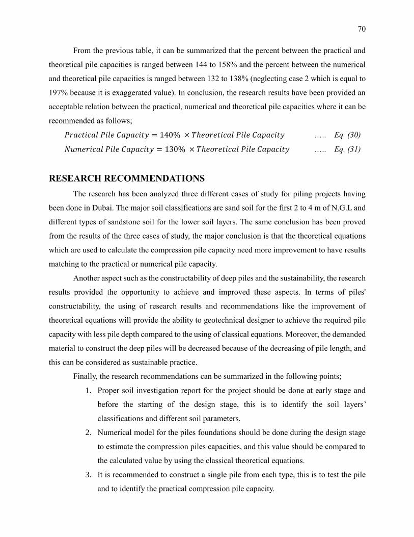
70
From the previous table, it can be summarized that the percent between the practical and
theoretical pile capacities is ranged between 144 to 158% and the percent between the numerical
and theoretical pile capacities is ranged between 132 to 138% (neglecting case 2 which is equal to
197% because it is exaggerated value). In conclusion, the research results have been provided an
acceptable relation between the practical, numerical and theoretical pile capacities where it can be
recommended as follows;
𝑃𝑟𝑎𝑐𝑡𝑖𝑐𝑎𝑙 𝑃𝑖𝑙𝑒 𝐶𝑎𝑝𝑎𝑐𝑖𝑡𝑦 = 140% × 𝑇ℎ𝑒𝑜𝑟𝑒𝑡𝑖𝑐𝑎𝑙 𝑃𝑖𝑙𝑒 𝐶𝑎𝑝𝑎𝑐𝑖𝑡𝑦 ….. Eq. (30)
𝑁𝑢𝑚𝑒𝑟𝑖𝑐𝑎𝑙 𝑃𝑖𝑙𝑒 𝐶𝑎𝑝𝑎𝑐𝑖𝑡𝑦 = 130% × 𝑇ℎ𝑒𝑜𝑟𝑒𝑡𝑖𝑐𝑎𝑙 𝑃𝑖𝑙𝑒 𝐶𝑎𝑝𝑎𝑐𝑖𝑡𝑦 ….. Eq. (31)
RESEARCH RECOMMENDATIONS
The research has been analyzed three different cases of study for piling projects having
been done in Dubai. The major soil classifications are sand soil for the first 2 to 4 m of N.G.L and
different types of sandstone soil for the lower soil layers. The same conclusion has been proved
from the results of the three cases of study, the major conclusion is that the theoretical equations
which are used to calculate the compression pile capacity need more improvement to have results
matching to the practical or numerical pile capacity.
Another aspect such as the constructability of deep piles and the sustainability, the research
results provided the opportunity to achieve and improved these aspects. In terms of piles'
constructability, the using of research results and recommendations like the improvement of
theoretical equations will provide the ability to geotechnical designer to achieve the required pile
capacity with less pile depth compared to the using of classical equations. Moreover, the demanded
material to construct the deep piles will be decreased because of the decreasing of pile length, and
this can be considered as sustainable practice.
Finally, the research recommendations can be summarized in the following points;
1. Proper soil investigation report for the project should be done at early stage and
before the starting of the design stage, this is to identify the soil layers’
classifications and different soil parameters.
2. Numerical model for the piles foundations should be done during the design stage
to estimate the compression piles capacities, and this value should be compared to
the calculated value by using the classical theoretical equations.
3. It is recommended to construct a single pile from each type, this is to test the pile
and to identify the practical compression pile capacity.
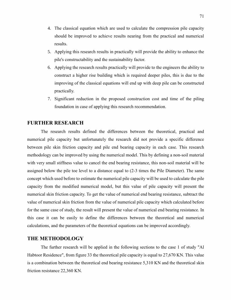
71
4. The classical equation which are used to calculate the compression pile capacity
should be improved to achieve results nearing from the practical and numerical
results.
5. Applying this research results in practically will provide the ability to enhance the
pile's constructability and the sustainability factor.
6. Applying the research results practically will provide to the engineers the ability to
construct a higher rise building which is required deeper piles, this is due to the
improving of the classical equations will end up with deep pile can be constructed
practically.
7. Significant reduction in the proposed construction cost and time of the piling
foundation in case of applying this research recommendation.
FURTHER RESEARCH
The research results defined the differences between the theoretical, practical and
numerical pile capacity but unfortunately the research did not provide a specific difference
between pile skin friction capacity and pile end bearing capacity in each case. This research
methodology can be improved by using the numerical model. This by defining a non-soil material
with very small stiffness value to cancel the end bearing resistance, this non-soil material will be
assigned below the pile toe level to a distance equal to (2-3 times the Pile Diameter). The same
concept which used before to estimate the numerical pile capacity will be used to calculate the pile
capacity from the modified numerical model, but this value of pile capacity will present the
numerical skin friction capacity. To get the value of numerical end bearing resistance, subtract the
value of numerical skin friction from the value of numerical pile capacity which calculated before
for the same case of study, the result will present the value of numerical end bearing resistance. In
this case it can be easily to define the differences between the theoretical and numerical
calculations, and the parameters of the theoretical equations can be improved accordingly.
THE METHODOLOGY
The further research will be applied in the following sections to the case 1 of study "Al
Habtoor Residence", from figure 33 the theoretical pile capacity is equal to 27,670 KN. This value
is a combination between the theoretical end bearing resistance 5,310 KN and the theoretical skin
friction resistance 22,360 KN.
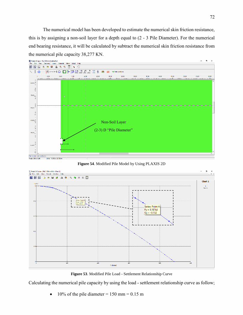
72
The numerical model has been developed to estimate the numerical skin friction resistance,
this is by assigning a non-soil layer for a depth equal to (2 - 3 Pile Diameter). For the numerical
end bearing resistance, it will be calculated by subtract the numerical skin friction resistance from
the numerical pile capacity 38,277 KN.
Calculating the numerical pile capacity by using the load - settlement relationship curve as follow;
10% of the pile diameter = 150 mm = 0.15 m
Figure 54. Modified Pile Model by Using PLAXIS 2D
Non-Soil Layer
(2-3) D “Pile Diameter”
Figure 53. Modified Pile Load - Settlement Relationship Curve

73
From the previous figure, Fy = 8,187 KN/rad at displacement equal to 120 mm
𝑄𝑈𝑆 = 𝐹𝑦 × 2𝜋 = 8,187 × 2𝜋 = 51,461 𝐾𝑁 ….. Eq. (32)
𝑄𝑆 = 𝑄𝑈
𝐹.𝑂.𝑆=
51,461
2= 25,730 𝐾𝑁 ….. Eq. (33)
From the previous equations, the calculated numerical skin friction compression pile capacity by
using PLAXIS 2D is 25,730 KN. The numerical end bearing resistance will be;
𝑄𝐵 = 𝑄 − 𝑄𝑆 = 38,277 − 25,730 = 12,547 𝐾𝑁 ….. Eq. (34)
The following table and figure summarized the results of the further research methodology;
Table 21. Further research results
CASE 1 _ AL HABTOOR RESIDENCE [Further Research]
Theoretical Capacity [KN] Numerical Capacity [KN]
27,670 38,277
% (Numerical / Theoretical) 138%
Theoretical Skin
Friction Capacity [KN]
Theoretical End
Bearing Capacity [KN]
Numerical Skin
Friction Capacity [KN]
Numerical End
Bearing Capacity [KN]
22,360 5,310 25,730 12,547
% (Numerical / Theoretical) 115% 236%
Figure 55. Further research results
22,360
5,310
25,730
12,547
0
5,000
10,000
15,000
20,000
25,000
30,000
Pil
e C
apac
ity [
KN
]
Pile Capacity Type
CASE 1 _ AL HABTOOR RESIDENCE [Further Research]
Theoretical Skin Friction Capacity [KN] Theoretical End Bearing Capacity [KN]
Numerical Skin Friction Capacity [KN] Numerical End Bearing Capacity [KN]
74
REFERENCES
1. Baker, B. & Pawlikowski, J. (2015). The Design and Construction of the World's Tallest
Building: The Burj Khalifa, Dubai. Structural Engineering International, vol. 25 (4), pp.
389-394.
2. Belloc, H. (1967). On. Freeport, N.Y.:Books for Libraries Press.
3. Brain, M. (n.d.). The engineering book.
4. Brinkgreve, R., Broere, W. & Al-Khoury, R. (2004). PLAXIS: 2D, version 8.
Lisse:Balkema.
5. Esrig, M. & Bachus, R. (1991). Deep foundation improvements. Philadelphia, Pa:American
Society for Testing and Materials.
6. Fu, F. (n.d.). Advanced Modeling Techniques in Structural Design.
7. Green, H. (1961). Long-Term Loading of Short-Bored Piles. Géotechnique, vol. 11 (1), pp.
47-53.
8. Hansbo, S. (1994). Foundation engineering. Amsterdam:Elsevier.
9. Huang, J., Zhang, J. & Chen, Z. (2011). Load-Transfer Properties of Extra-Long Piles
Embedded into Deep Hard-Rock and High-Pressure Grouting Piles Set into Fragmental
Rock. Advanced Materials Research, vol. 250-253, pp. 2501-2505.
10. Johnson, A. (2013). Recommendations on Piling (EA Pfhle). Hoboken:Wiley.
11. Lee, M. (2015). How did they build that?. La Jolla, CA:Scobre Educational.
12. Lin, M. (2006). Proceedings of the International Symposium on New Generation Design
Codes for Geotechnical Engineering Practice - Taipei 2006. Singapore:World Scientific.
13. Murthy, V. (2003). Geotechnical engineering. New York:Marcel Dekker.
14. Tomlinson, M. & Boorman, R. (2001). Foundation design and construction. Harlow
[u.a.]:Prentice Hall.
15. Tomlinson, M. & Woodward, J. (n.d.). Pile design and construction practice.
16. Vesic, A. (1977). Design of pile foundations. Washington:Transportation Research Board,
National Research Council.
75
17. Advances in structural engineering. (2011). Durnten-Zurich:TTP, Trans Tech Publications.
18. Bowles, J. (2007). Foundation analysis and design. Norwich, NY:Knovel.
19. British Standard code of practice for foundations (formerly CP 2004). (1986).
London:British Standards Institution.
20. Chang, S., Bahar, S. & Zhao, J. (2013). Advances in civil engineering and building materals.
Boca Raton, Fla.:CRC Press.
21. Chen, F. & Morris, M. (2001). Soil engineering. Boca Raton:CRC Press.
22. Cock, F. & Legrand, C. (1997). Design of axially loaded piles. Rotterdam [u.a.]:Balkema.
23. Design and construction of auger cast piles, and other foundation issues. (1994).
Washington, D.C.:National Academy Press.
24. Hamza, M., Shahien, M. & El-Mossallamy, Y. (2009). Proceedings of the 17th International
Conference on Soil Mechanics and Geotechnical Engineering. Amsterdam:IOS Press /
Millpress Science Pub.
25. Madabhushi, G., Knappett, J. & Haigh, S. (2010). Design of pile foundations in liquefiable
soils. London:Imperial College Press.
26. Orense, R., Chouw, N. & Pender, M. (2010). Soil-Foundation-Structure Interaction.
Abingdon:CRC Press [Imprint].
27. Soil mechanics 2006. (2006). Washington:Transportation Research Board.
28. Terzaghi, K. (2007). Theoretical Soil Mechanics. Hoboken:Wiley [Imprint].
29. Young, F. (1982). Piles and foundations. London:Telford.
30. Zhao, Z., Chai, J. & Fan, C. (2014). Numerical Simulation Analysis of Bearing
Performance of Extra-Long and Large-Diameter Single Pile. Advanced Materials Research,
vol. 1065-1069, pp. 943-948.
31. Aoyama, H. (2001). Design of modern highrise reinforced concrete structures.
London:Imperial College Press.
32. Belloc, H. (1967). On. Freeport, N.Y.:Books for Libraries Press.
33. Belloc, H. (1967). On. Freeport, N.Y.:Books for Libraries Press.
76
34. Bowles, J. (2007). Foundation analysis and design. Norwich, NY:Knovel.
35. Coduto, D., Kitch, W. & Yeung, M. (n.d.). Foundation design.
36. Crowther, C. (1989). Load testing of deep foundations. New York:Wiley.
37. Meyer, J. (1984). Analysis and design of pile foundations. New York, N.Y.:American
Society of Civil Engineers.
38. Nash, P. (1989). Super structures. Ada, OK:Garrett Educational Corp.
39. Rao, N. (2011). Foundation Design: Theory and Practice. John Wiley & Sons.
40. Sabry, M. (2002). Shaft resistance of a single vertical or batter pile in sand subjected to
axial compression or uplift loading. Ottawa:National Library of Canada = Bibliotheque
nationale du Canada.
41. Wolf, J. & Deeks, A. (2004). Foundation vibration analysis. Amsterdam [u.a.]:Elsevier.
42. Wrana, B. (2015). Pile Load Capacity – Calculation Methods. Studia Geotechnica et
Mechanica, vol. 37 (4).
43. Coduto, D., Kitch, W. & Yeung, M. (n.d.). Foundation design.
44. Deep Foundations on Bored and Auger Piles - BAP V. (2008). CRC Press.
45. Fleming, W. & Sliwinski, Z. (1986). The use and influence of bentonite in bored pile
construction. London:CIRIA.
46. Gong, X., Fan, Q. & Xu, Y. (2011). Efficiency of Pile Groups of Large Diameter Bored
Cast-in-Place Pile. Advanced Materials Research, vol. 261-263, pp. 1215-1219.
47. Wulandari, P. & Tjandra, D. (2015). Analysis of Piled Raft Foundation on Soft Soil Using
PLAXIS 2D. Procedia Engineering, vol. 125, pp. 363-367.
48. 孙, 永. (2013). Based on PLAXIS Finite Element Software Analysis of Deep Foundation
Pit. Hans Journal of Civil Engineering, vol. 02 (02), pp. 110-121.

77
Appendix [1] – Numerical Models Output

78
Numerical Models Output [Case 1]

REPORT
10/09/2017
User: Koxhiyoki Kabuto, Japan
Title: PILE 1500mm
PLAXIS 8.x Professional version
2
Table of Contents
1. General Information .......................................................................................................................................... 3
2. Geometry ........................................................................................................................................................... 4
2.1. Clusters ....................................................................................................................................................... 5
3. Structures .......................................................................................................................................................... 6
4. Mesh data .......................................................................................................................................................... 7
5. Material data ..................................................................................................................................................... 8

PLAXIS 8.x Professional version
3
1. General Information Table [1] units
Type Unit
Length
Force
Time
m
kN
day
Table [2] Model dimensions
min. max.
X
Y
0.000
-130.000
104.000
0.000
Table [3] Model
Model Axisymmetry
Element 15-Noded
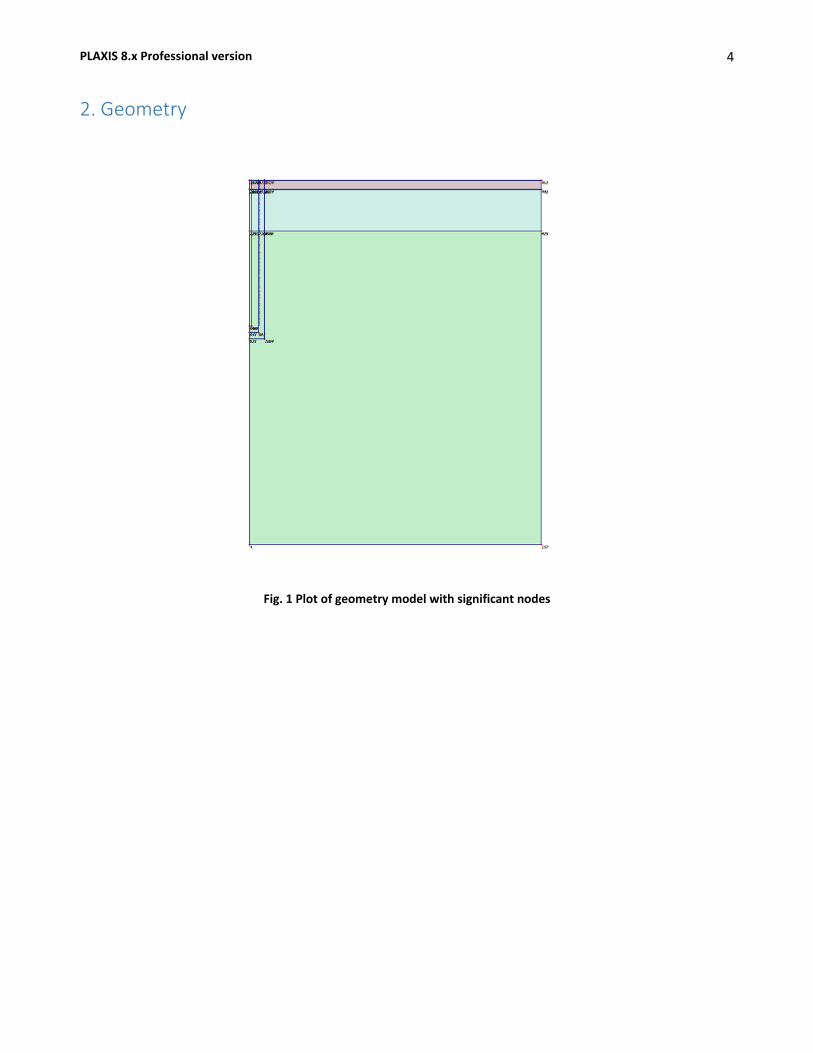
PLAXIS 8.x Professional version
4
2. Geometry
Fig. 1 Plot of geometry model with significant nodes

PLAXIS 8.x Professional version
5
2.1. Clusters
Fig. 2 Plot of geometry model with cluster numbers
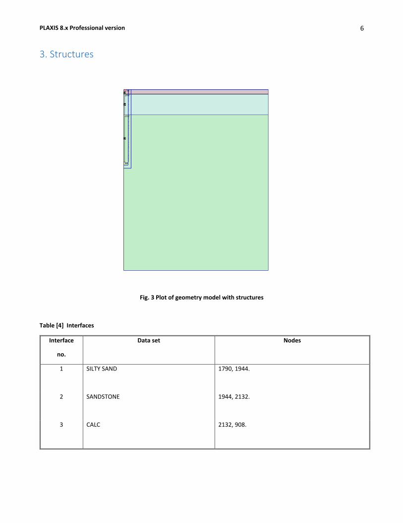
PLAXIS 8.x Professional version
6
3. Structures
Fig. 3 Plot of geometry model with structures
Table [4] Interfaces
Interface
no.
Data set Nodes
1 SILTY SAND
1790, 1944.
2 SANDSTONE
1944, 2132.
3 CALC
2132, 908.
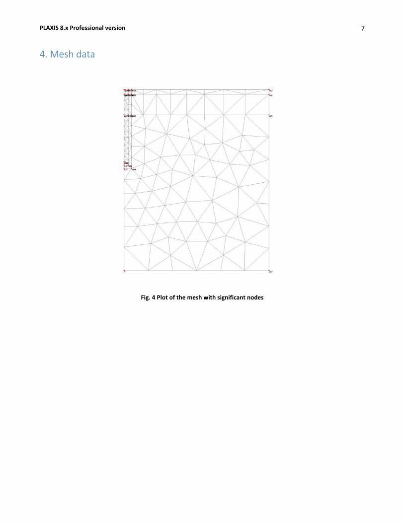
PLAXIS 8.x Professional version
7
4. Mesh data
Fig. 4 Plot of the mesh with significant nodes
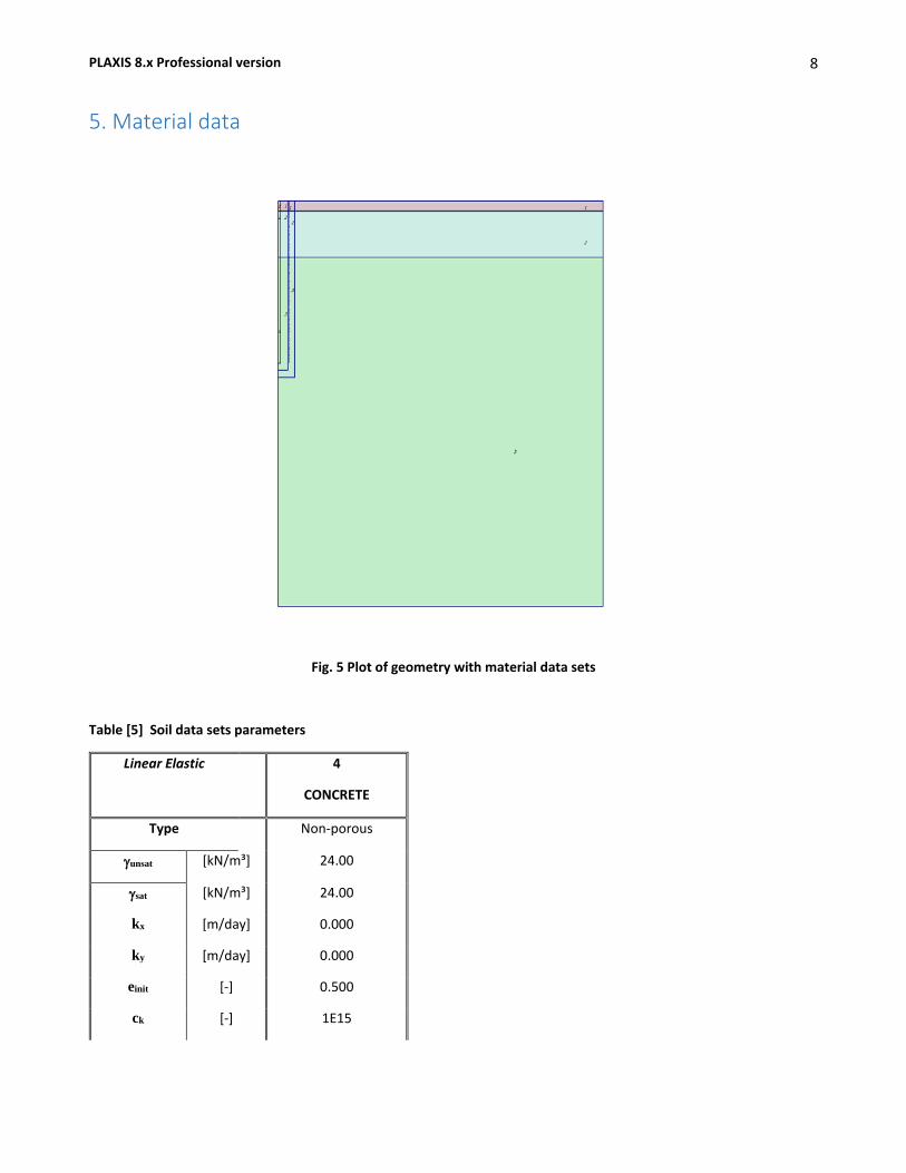
PLAXIS 8.x Professional version
8
5. Material data
Fig. 5 Plot of geometry with material data sets
Table [5] Soil data sets parameters
Linear Elastic
4
CONCRETE
Type Non-porous
γunsat [kN/m³] 24.00
γsat [kN/m³] 24.00
kx [m/day] 0.000
ky [m/day] 0.000
einit [-] 0.500
ck [-] 1E15

PLAXIS 8.x Professional version
9
Linear Elastic
4
CONCRETE
Eref [kN/m²] 31992382.14
ν [-] 0.200
Gref [kN/m²] 13329524.082
Eoed [kN/m²] 35549632.653
Eincr [kN/m²/m]
0.00
yref [m] 0.000
Rinter [-] 1.000
Interface
permeability
Impermeable
Mohr-Coulomb
1
SILTY SAND
2
SANDSTONE
3
CALC
Type Drained Drained Drained
γunsat [kN/m³] 18.50 19.00 19.50
γsat [kN/m³] 18.50 19.00 19.50
kx [m/day] 1.000 0.500 0.500
ky [m/day] 1.000 0.500 0.500
einit [-] 0.500 0.500 0.500
ck [-] 1E15 1E15 1E15
Eref [kN/m²] 30000.000 200000.000 400000.000
ν [-] 0.300 0.300 0.300
Gref [kN/m²] 11540.645 76929.047 153857.001
Eoed [kN/m²] 40356.820 269154.702 538323.312
cref [kN/m²] 5.00 40.00 60.00
ϕ [°] 34.00 40.00 40.00
ψ [°] 5.00 10.00 10.00
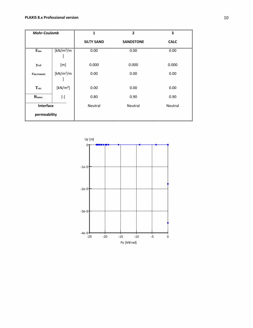
PLAXIS 8.x Professional version
10
Mohr-Coulomb
1
SILTY SAND
2
SANDSTONE
3
CALC
Einc [kN/m²/m]
0.00 0.00 0.00
yref [m] 0.000 0.000 0.000
cincrement [kN/m²/m]
0.00 0.00 0.00
Tstr. [kN/m²] 0.00 0.00 0.00
Rinter. [-] 0.80 0.90 0.90
Interface
permeability
Neutral Neutral Neutral
-25 -20 -15 -10 -5 0-4e-5
-3e-5
-2e-5
-1e-5
0
Fy [kN/rad]
Uy [m]
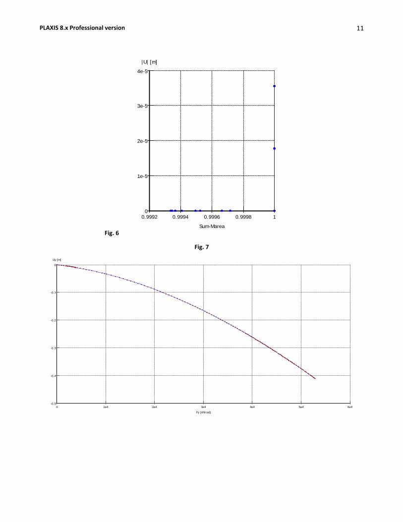
PLAXIS 8.x Professional version
11
Fig. 6
Fig. 7
0.9992 0.9994 0.9996 0.9998 10
1e-5
2e-5
3e-5
4e-5
Sum-Marea
|U| [m]
0 1e4 2e4 3e4 4e4 5e4 6e4-0.5
-0.4
-0.3
-0.2
-0.1
0
Fy [kN/rad]
Uy [m]
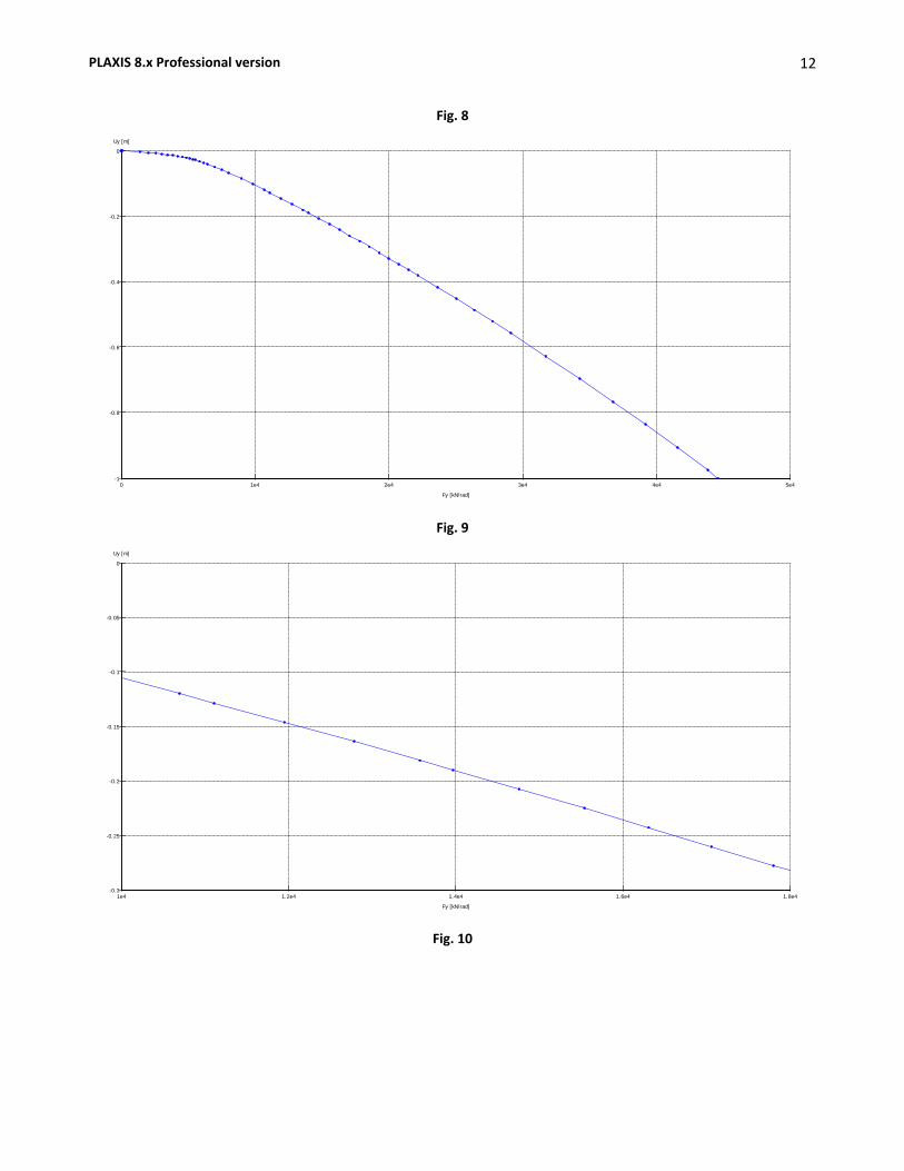
PLAXIS 8.x Professional version
12
Fig. 8
Fig. 9
Fig. 10
0 1e4 2e4 3e4 4e4 5e4-1
-0.8
-0.6
-0.4
-0.2
0
Fy [kN/rad]
Uy [m]
1e4 1.2e4 1.4e4 1.6e4 1.8e4-0.3
-0.25
-0.2
-0.15
-0.1
-0.05
0
Fy [kN/rad]
Uy [m]

79
Numerical Models Output [Case 2]

REPORT
10/09/2017
User: Koxhiyoki Kabuto, Japan
Title:

PLAXIS 8.x Professional version
2
Table of Contents
1. General Information .......................................................................................................................................... 3
2. Geometry ........................................................................................................................................................... 4
2.1. Clusters ....................................................................................................................................................... 5
3. Structures .......................................................................................................................................................... 6
4. Mesh data .......................................................................................................................................................... 8
5. Material data ..................................................................................................................................................... 9

PLAXIS 8.x Professional version
3
1. General Information Table [1] units
Type Unit
Length
Force
Time
m
kN
day
Table [2] Model dimensions
min. max.
X
Y
0.000
-85.000
68.000
0.000
Table [3] Model
Model Axisymmetry
Element 15-Noded
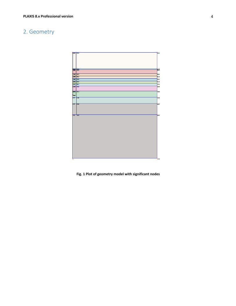
PLAXIS 8.x Professional version
4
2. Geometry
Fig. 1 Plot of geometry model with significant nodes
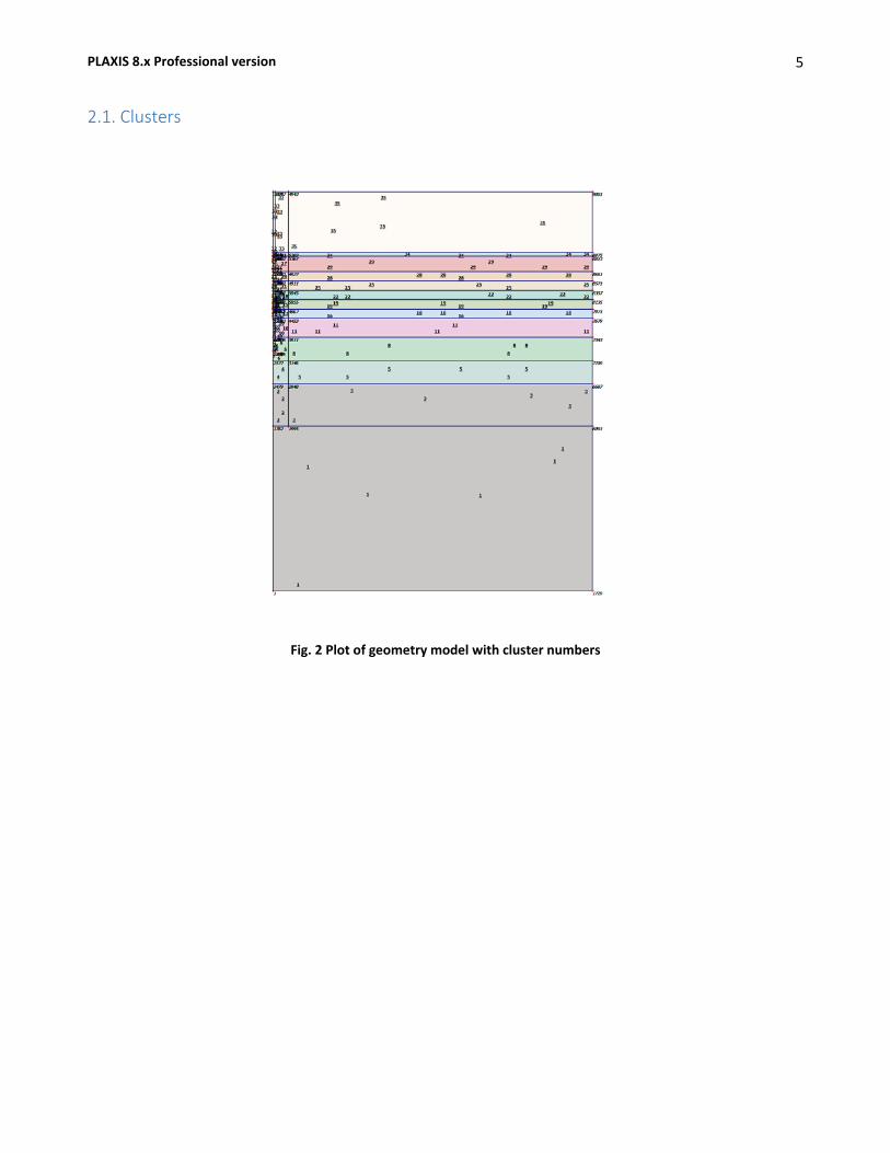
PLAXIS 8.x Professional version
5
2.1. Clusters
Fig. 2 Plot of geometry model with cluster numbers
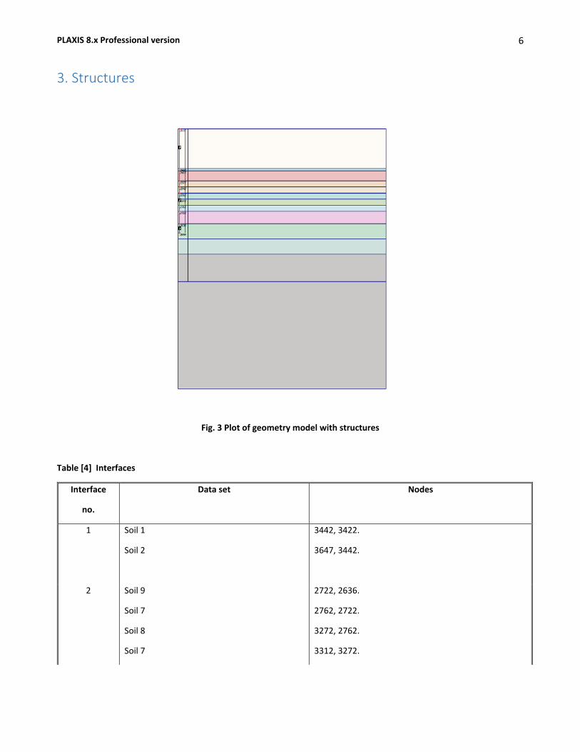
PLAXIS 8.x Professional version
6
3. Structures
Fig. 3 Plot of geometry model with structures
Table [4] Interfaces
Interface
no.
Data set Nodes
1 Soil 1
Soil 2
3442, 3422.
3647, 3442.
2 Soil 9
Soil 7
Soil 8
Soil 7
2722, 2636.
2762, 2722.
3272, 2762.
3312, 3272.
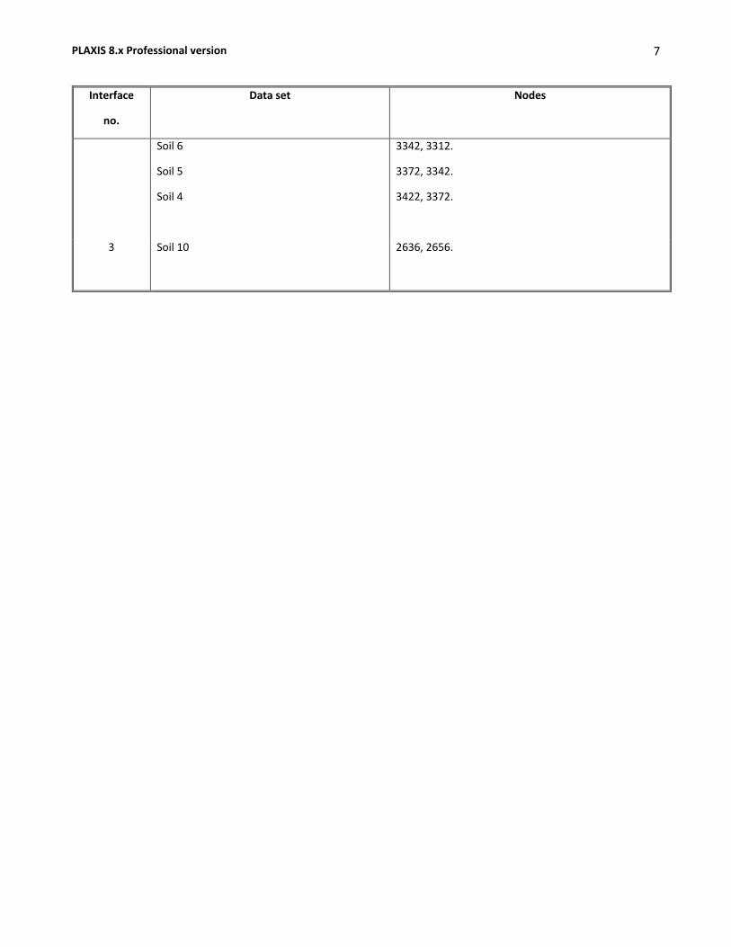
PLAXIS 8.x Professional version
7
Interface
no.
Data set Nodes
Soil 6
Soil 5
Soil 4
3342, 3312.
3372, 3342.
3422, 3372.
3 Soil 10
2636, 2656.
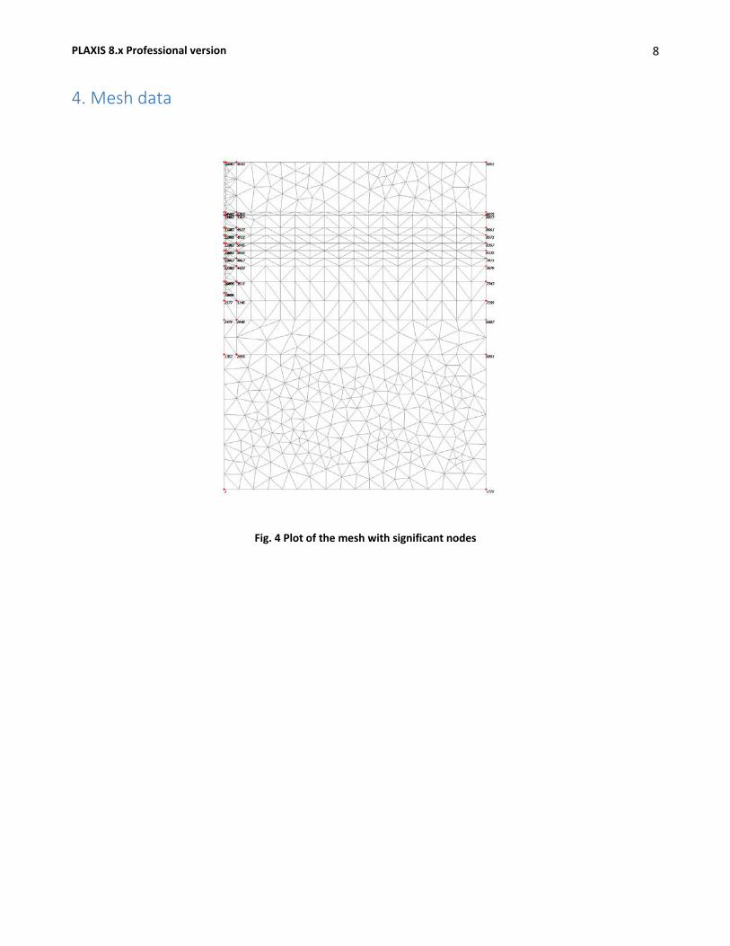
PLAXIS 8.x Professional version
8
4. Mesh data
Fig. 4 Plot of the mesh with significant nodes
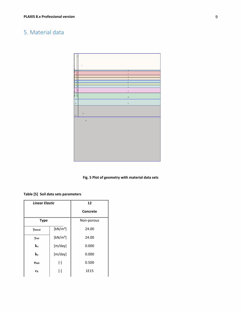
PLAXIS 8.x Professional version
9
5. Material data
Fig. 5 Plot of geometry with material data sets
Table [5] Soil data sets parameters
Linear Elastic
12
Concrete
Type Non-porous
γunsat [kN/m³] 24.00
γsat [kN/m³] 24.00
kx [m/day] 0.000
ky [m/day] 0.000
einit [-] 0.500
ck [-] 1E15
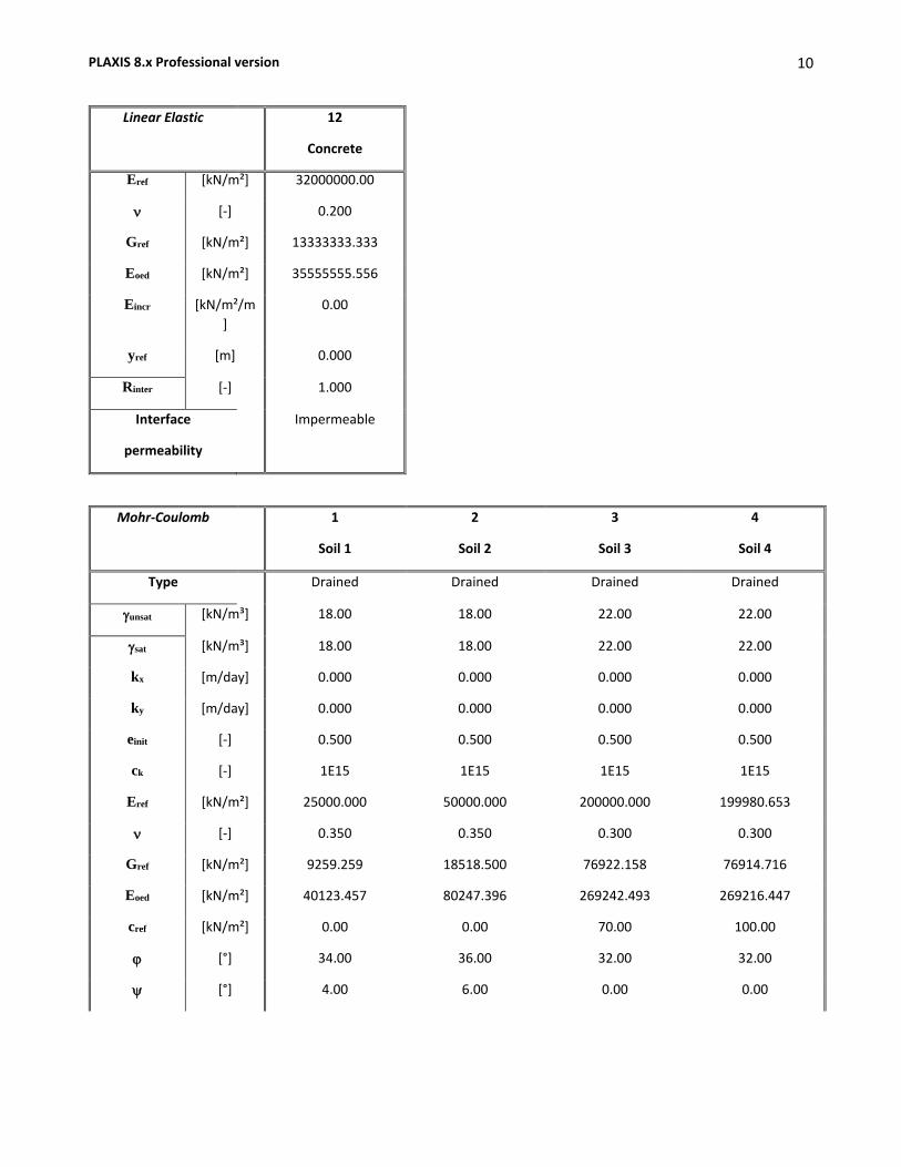
PLAXIS 8.x Professional version
10
Linear Elastic
12
Concrete
Eref [kN/m²] 32000000.00
ν [-] 0.200
Gref [kN/m²] 13333333.333
Eoed [kN/m²] 35555555.556
Eincr [kN/m²/m]
0.00
yref [m] 0.000
Rinter [-] 1.000
Interface
permeability
Impermeable
Mohr-Coulomb
1
Soil 1
2
Soil 2
3
Soil 3
4
Soil 4
Type Drained Drained Drained Drained
γunsat [kN/m³] 18.00 18.00 22.00 22.00
γsat [kN/m³] 18.00 18.00 22.00 22.00
kx [m/day] 0.000 0.000 0.000 0.000
ky [m/day] 0.000 0.000 0.000 0.000
einit [-] 0.500 0.500 0.500 0.500
ck [-] 1E15 1E15 1E15 1E15
Eref [kN/m²] 25000.000 50000.000 200000.000 199980.653
ν [-] 0.350 0.350 0.300 0.300
Gref [kN/m²] 9259.259 18518.500 76922.158 76914.716
Eoed [kN/m²] 40123.457 80247.396 269242.493 269216.447
cref [kN/m²] 0.00 0.00 70.00 100.00
ϕ [°] 34.00 36.00 32.00 32.00
ψ [°] 4.00 6.00 0.00 0.00
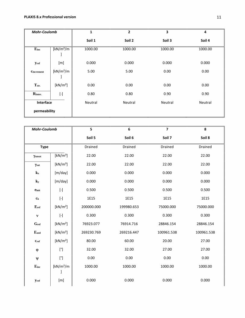
PLAXIS 8.x Professional version
11
Mohr-Coulomb
1
Soil 1
2
Soil 2
3
Soil 3
4
Soil 4
Einc [kN/m²/m]
1000.00 1000.00 1000.00 1000.00
yref [m] 0.000 0.000 0.000 0.000
cincrement [kN/m²/m]
5.00 5.00 0.00 0.00
Tstr. [kN/m²] 0.00 0.00 0.00 0.00
Rinter. [-] 0.80 0.80 0.90 0.90
Interface
permeability
Neutral Neutral Neutral Neutral
Mohr-Coulomb
5
Soil 5
6
Soil 6
7
Soil 7
8
Soil 8
Type Drained Drained Drained Drained
γunsat [kN/m³] 22.00 22.00 22.00 22.00
γsat [kN/m³] 22.00 22.00 22.00 22.00
kx [m/day] 0.000 0.000 0.000 0.000
ky [m/day] 0.000 0.000 0.000 0.000
einit [-] 0.500 0.500 0.500 0.500
ck [-] 1E15 1E15 1E15 1E15
Eref [kN/m²] 200000.000 199980.653 75000.000 75000.000
ν [-] 0.300 0.300 0.300 0.300
Gref [kN/m²] 76923.077 76914.716 28846.154 28846.154
Eoed [kN/m²] 269230.769 269216.447 100961.538 100961.538
cref [kN/m²] 80.00 60.00 20.00 27.00
ϕ [°] 32.00 32.00 27.00 27.00
ψ [°] 0.00 0.00 0.00 0.00
Einc [kN/m²/m]
1000.00 1000.00 1000.00 1000.00
yref [m] 0.000 0.000 0.000 0.000

PLAXIS 8.x Professional version
12
Mohr-Coulomb
5
Soil 5
6
Soil 6
7
Soil 7
8
Soil 8
cincrement [kN/m²/m]
0.00 0.00 0.00 0.00
Tstr. [kN/m²] 0.00 0.00 0.00 0.00
Rinter. [-] 0.90 0.90 0.90 0.90
Interface
permeability
Neutral Neutral Neutral Neutral
Mohr-Coulomb
9
Soil 9
10
Soil 10
11
Soil 11
13
Soil 12
Type Drained Drained Drained Drained
γunsat [kN/m³] 22.00 22.00 22.00 22.00
γsat [kN/m³] 22.00 22.00 22.00 22.00
kx [m/day] 0.000 0.000 0.000 0.000
ky [m/day] 0.000 0.000 0.000 0.000
einit [-] 0.500 0.500 0.500 0.500
ck [-] 1E15 1E15 1E15 1E15
Eref [kN/m²] 149982.587 250081.119 250000.000 400051.358
ν [-] 0.300 0.300 0.300 0.300
Gref [kN/m²] 57685.100 96191.633 96153.846 153863.600
Eoed [kN/m²] 201906.145 336563.722 336538.462 538560.090
cref [kN/m²] 60.00 120.00 130.00 85.00
ϕ [°] 32.00 32.00 32.00 34.00
ψ [°] 0.00 0.00 0.00 0.00
Einc [kN/m²/m]
1000.00 1000.00 1000.00 1000.00
yref [m] 0.000 0.000 0.000 0.000
cincrement [kN/m²/m]
0.00 0.00 0.00 0.00
Tstr. [kN/m²] 0.00 0.00 0.00 0.00
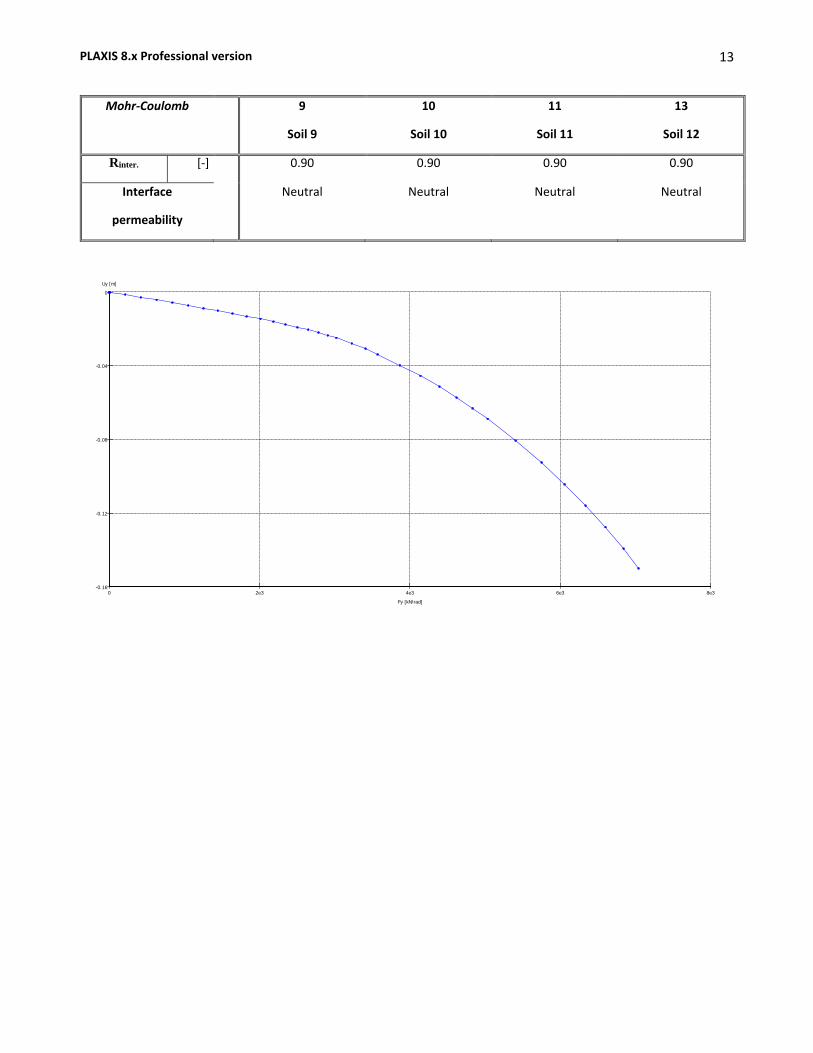
PLAXIS 8.x Professional version
13
Mohr-Coulomb
9
Soil 9
10
Soil 10
11
Soil 11
13
Soil 12
Rinter. [-] 0.90 0.90 0.90 0.90
Interface
permeability
Neutral Neutral Neutral Neutral
0 2e3 4e3 6e3 8e3
-0.16
-0.12
-0.08
-0.04
0
Fy [kN/rad]
Uy [m]
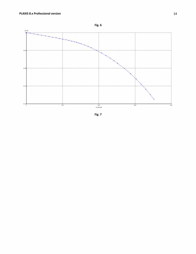
PLAXIS 8.x Professional version
14
Fig. 6
Fig. 7
0 2e3 4e3 6e3 8e3-0.16
-0.12
-0.08
-0.04
0
Fy [kN/rad]
Uy [m]

80
Numerical Models Output [Case 3]

REPORT
10/09/2017
User: Koxhiyoki Kabuto, Japan
Title: Pile Dia 1200 mm

PLAXIS 8.x Professional version
2
Table of Contents
1. General Information .......................................................................................................................................... 3
2. Geometry ........................................................................................................................................................... 4
2.1. Clusters ....................................................................................................................................................... 5
3. Structures .......................................................................................................................................................... 6
4. Mesh data .......................................................................................................................................................... 8
5. Material data ..................................................................................................................................................... 9
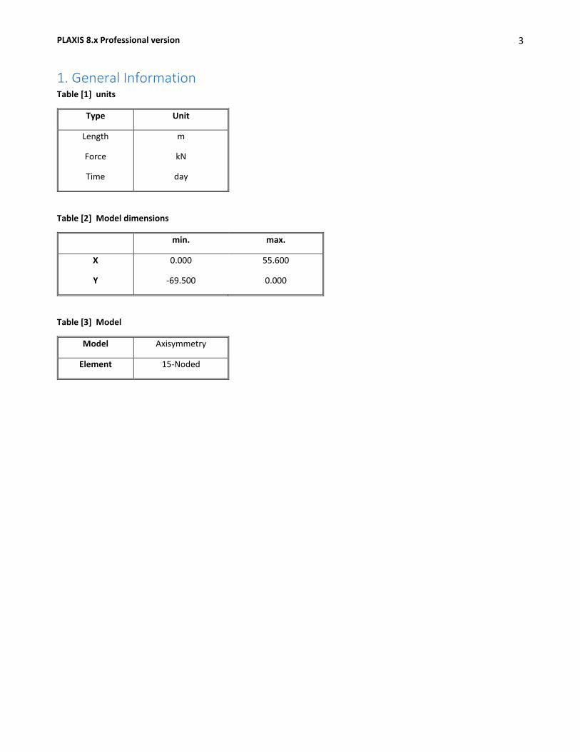
PLAXIS 8.x Professional version
3
1. General Information Table [1] units
Type Unit
Length
Force
Time
m
kN
day
Table [2] Model dimensions
min. max.
X
Y
0.000
-69.500
55.600
0.000
Table [3] Model
Model Axisymmetry
Element 15-Noded
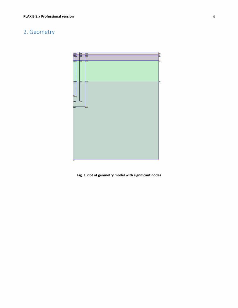
PLAXIS 8.x Professional version
4
2. Geometry
Fig. 1 Plot of geometry model with significant nodes
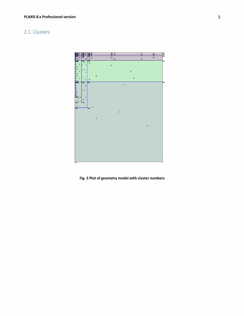
PLAXIS 8.x Professional version
5
2.1. Clusters
Fig. 2 Plot of geometry model with cluster numbers
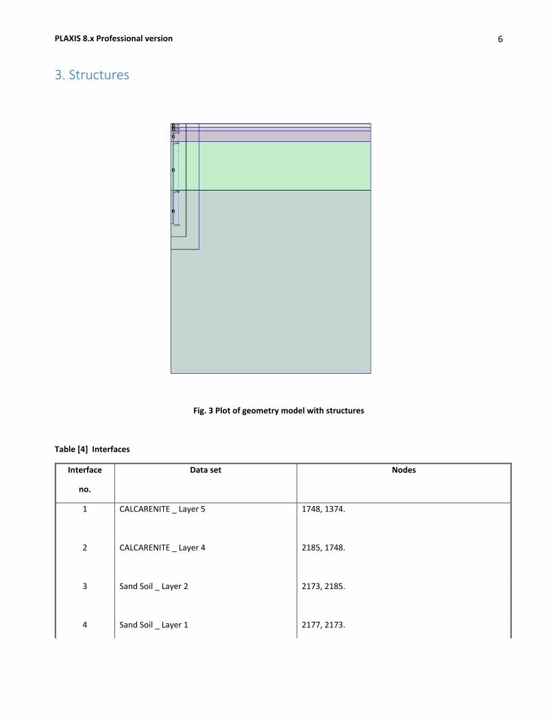
PLAXIS 8.x Professional version
6
3. Structures
Fig. 3 Plot of geometry model with structures
Table [4] Interfaces
Interface
no.
Data set Nodes
1 CALCARENITE _ Layer 5
1748, 1374.
2 CALCARENITE _ Layer 4
2185, 1748.
3 Sand Soil _ Layer 2
2173, 2185.
4 Sand Soil _ Layer 1 2177, 2173.

PLAXIS 8.x Professional version
7
Interface
no.
Data set Nodes
5 Sand Soil _ Layer 2
2147, 2177.
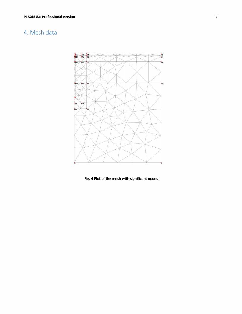
PLAXIS 8.x Professional version
8
4. Mesh data
Fig. 4 Plot of the mesh with significant nodes

PLAXIS 8.x Professional version
9
5. Material data
Fig. 5 Plot of geometry with material data sets
Table [5] Soil data sets parameters
Linear Elastic
6
Concrete
Type Non-porous
γunsat [kN/m³] 24.00
γsat [kN/m³] 24.00
kx [m/day] 0.000
ky [m/day] 0.000
einit [-] 0.500
ck [-] 1E15
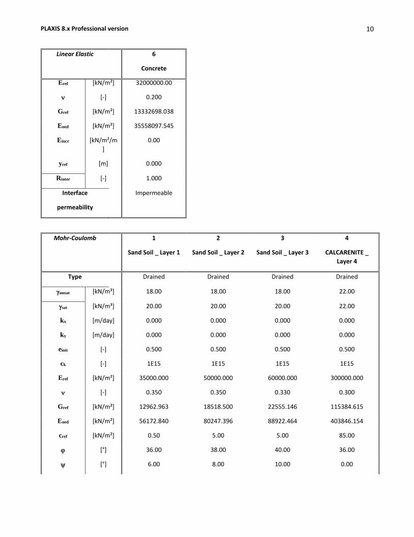
PLAXIS 8.x Professional version
10
Linear Elastic
6
Concrete
Eref [kN/m²] 32000000.00
ν [-] 0.200
Gref [kN/m²] 13332698.038
Eoed [kN/m²] 35558097.545
Eincr [kN/m²/m]
0.00
yref [m] 0.000
Rinter [-] 1.000
Interface
permeability
Impermeable
Mohr-Coulomb
1
Sand Soil _ Layer 1
2
Sand Soil _ Layer 2
3
Sand Soil _ Layer 3
4
CALCARENITE _ Layer 4
Type Drained Drained Drained Drained
γunsat [kN/m³] 18.00 18.00 18.00 22.00
γsat [kN/m³] 20.00 20.00 20.00 22.00
kx [m/day] 0.000 0.000 0.000 0.000
ky [m/day] 0.000 0.000 0.000 0.000
einit [-] 0.500 0.500 0.500 0.500
ck [-] 1E15 1E15 1E15 1E15
Eref [kN/m²] 35000.000 50000.000 60000.000 300000.000
ν [-] 0.350 0.350 0.330 0.300
Gref [kN/m²] 12962.963 18518.500 22555.146 115384.615
Eoed [kN/m²] 56172.840 80247.396 88922.464 403846.154
cref [kN/m²] 0.50 5.00 5.00 85.00
ϕ [°] 36.00 38.00 40.00 36.00
ψ [°] 6.00 8.00 10.00 0.00
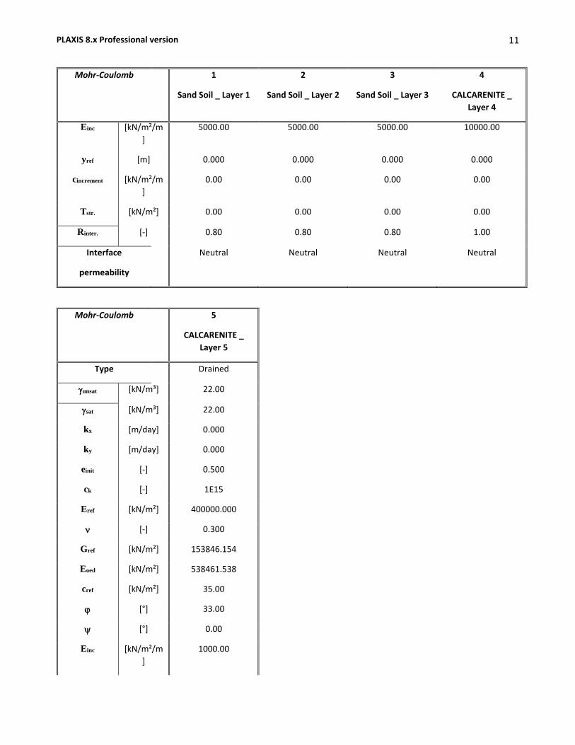
PLAXIS 8.x Professional version
11
Mohr-Coulomb
1
Sand Soil _ Layer 1
2
Sand Soil _ Layer 2
3
Sand Soil _ Layer 3
4
CALCARENITE _ Layer 4
Einc [kN/m²/m]
5000.00 5000.00 5000.00 10000.00
yref [m] 0.000 0.000 0.000 0.000
cincrement [kN/m²/m]
0.00 0.00 0.00 0.00
Tstr. [kN/m²] 0.00 0.00 0.00 0.00
Rinter. [-] 0.80 0.80 0.80 1.00
Interface
permeability
Neutral Neutral Neutral Neutral
Mohr-Coulomb
5
CALCARENITE _ Layer 5
Type Drained
γunsat [kN/m³] 22.00
γsat [kN/m³] 22.00
kx [m/day] 0.000
ky [m/day] 0.000
einit [-] 0.500
ck [-] 1E15
Eref [kN/m²] 400000.000
ν [-] 0.300
Gref [kN/m²] 153846.154
Eoed [kN/m²] 538461.538
cref [kN/m²] 35.00
ϕ [°] 33.00
ψ [°] 0.00
Einc [kN/m²/m]
1000.00
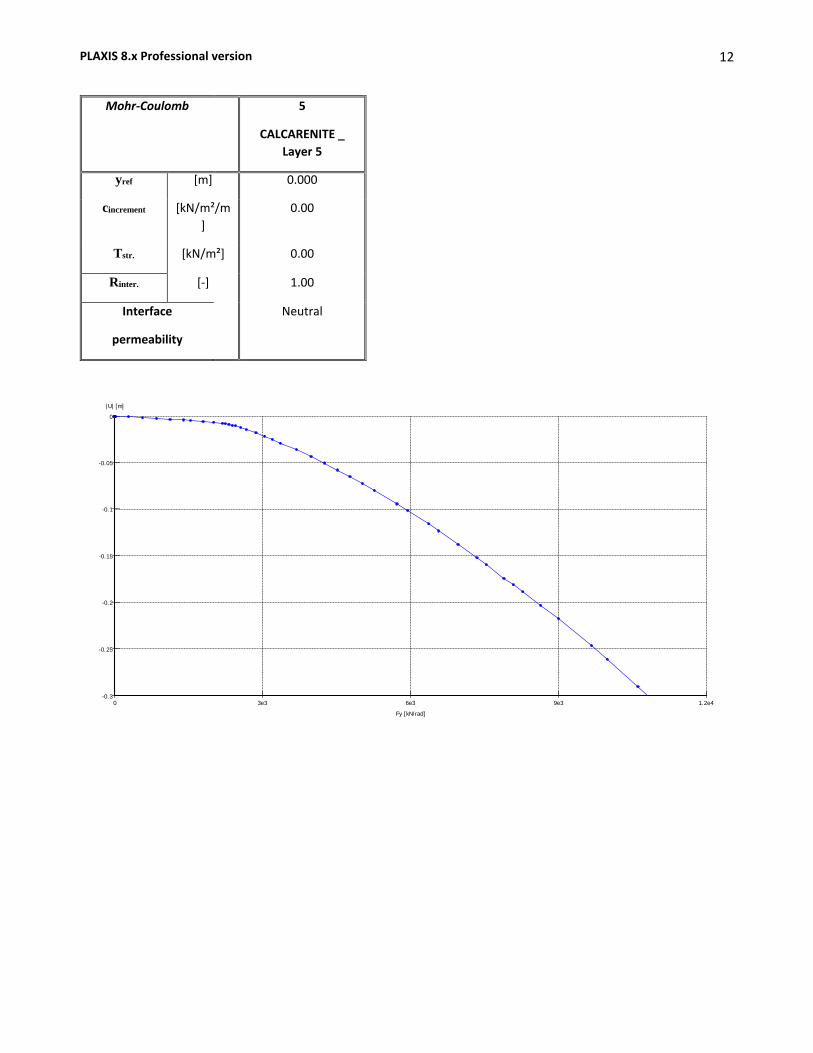
PLAXIS 8.x Professional version
12
Mohr-Coulomb
5
CALCARENITE _ Layer 5
yref [m] 0.000
cincrement [kN/m²/m]
0.00
Tstr. [kN/m²] 0.00
Rinter. [-] 1.00
Interface
permeability
Neutral
0 3e3 6e3 9e3 1.2e4
-0.3
-0.25
-0.2
-0.15
-0.1
-0.05
0
Fy [kN/rad]
|U| [m]
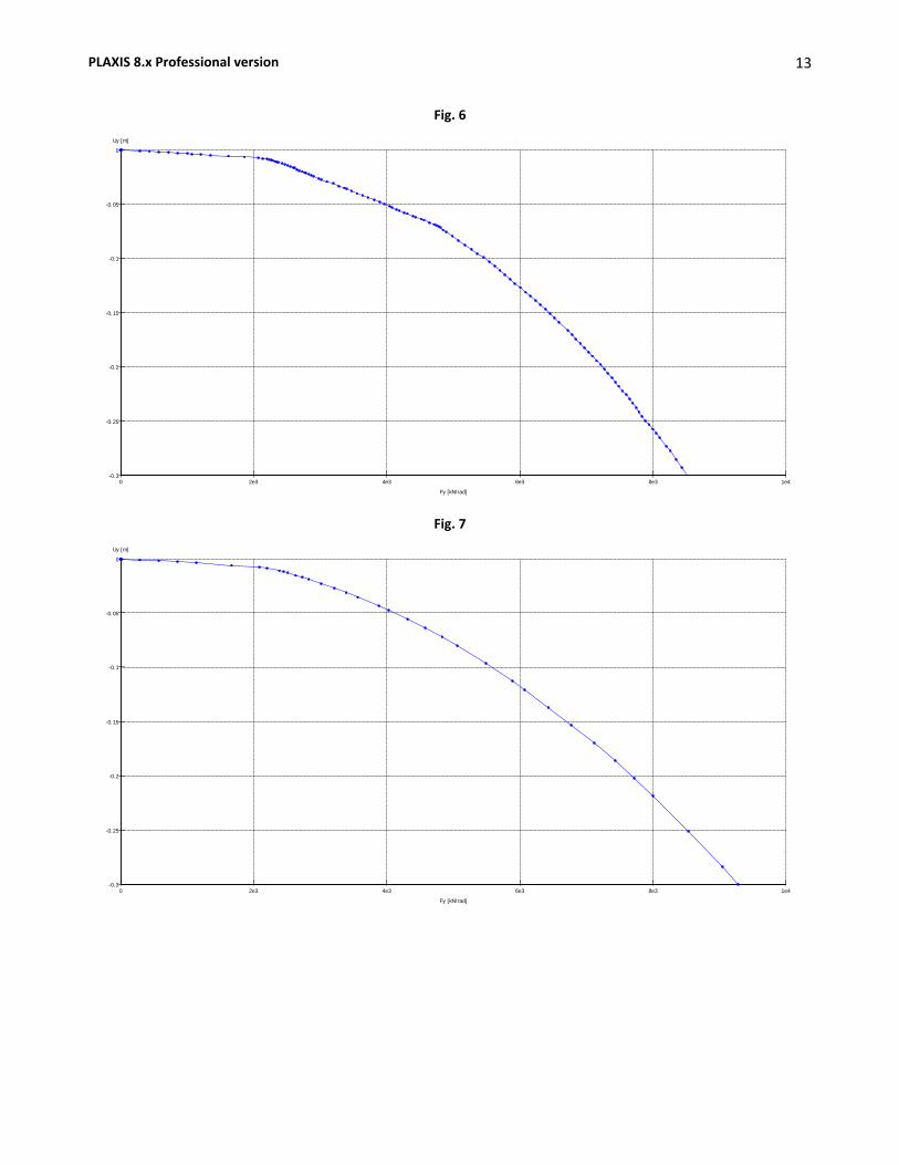
PLAXIS 8.x Professional version
13
Fig. 6
Fig. 7
0 2e3 4e3 6e3 8e3 1e4-0.3
-0.25
-0.2
-0.15
-0.1
-0.05
0
Fy [kN/rad]
Uy [m]
0 2e3 4e3 6e3 8e3 1e4-0.3
-0.25
-0.2
-0.15
-0.1
-0.05
0
Fy [kN/rad]
Uy [m]
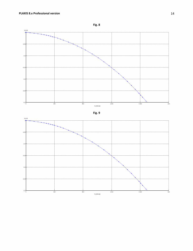
PLAXIS 8.x Professional version
14
Fig. 8
Fig. 9
0 4e3 8e3 1.2e4 1.6e4 2e4-0.3
-0.25
-0.2
-0.15
-0.1
-0.05
0
Fy [kN/rad]
Uy [m]
0 4e3 8e3 1.2e4 1.6e4 2e4-0.3
-0.25
-0.2
-0.15
-0.1
-0.05
0
Fy [kN/rad]
Uy [m]
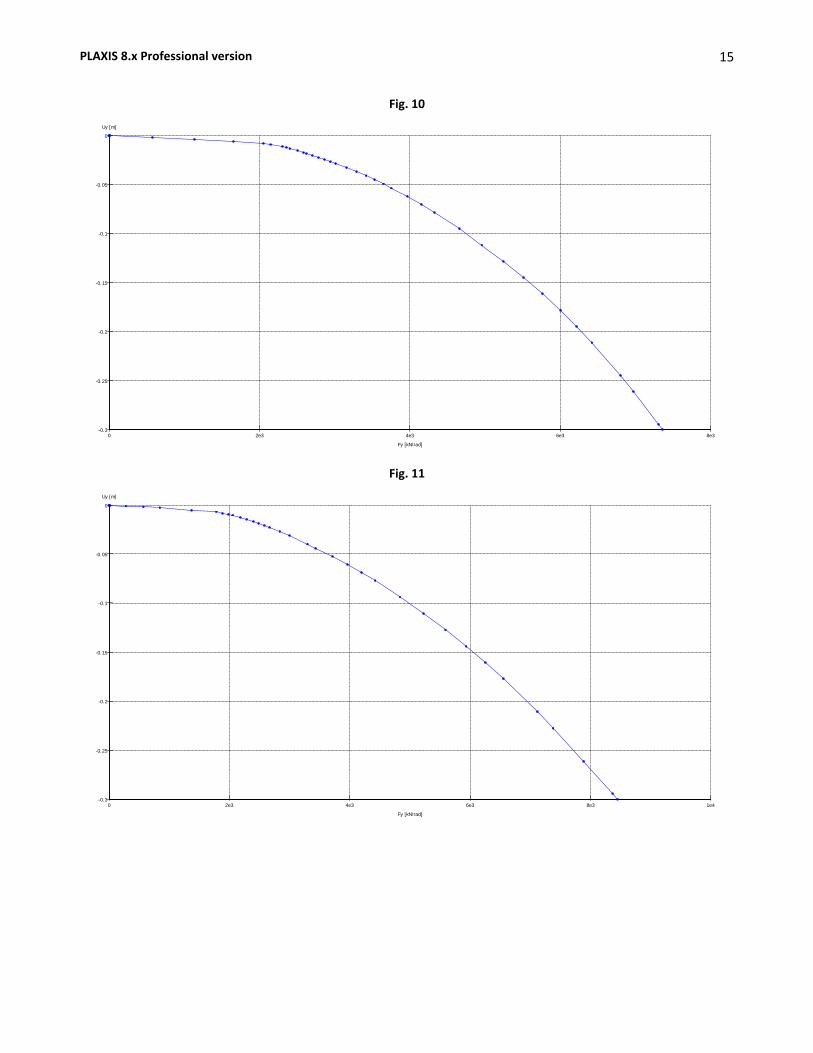
PLAXIS 8.x Professional version
15
Fig. 10
Fig. 11
0 2e3 4e3 6e3 8e3-0.3
-0.25
-0.2
-0.15
-0.1
-0.05
0
Fy [kN/rad]
Uy [m]
0 2e3 4e3 6e3 8e3 1e4-0.3
-0.25
-0.2
-0.15
-0.1
-0.05
0
Fy [kN/rad]
Uy [m]
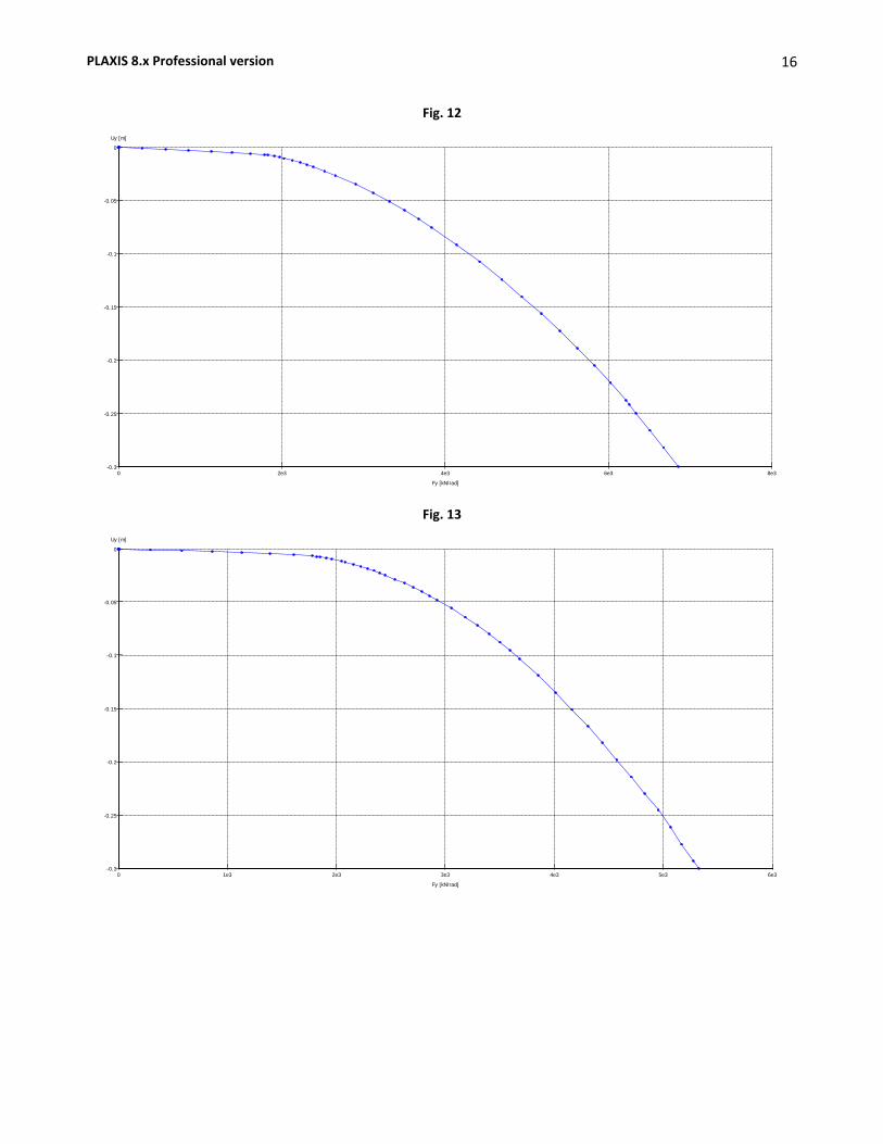
PLAXIS 8.x Professional version
16
Fig. 12
Fig. 13
0 2e3 4e3 6e3 8e3-0.3
-0.25
-0.2
-0.15
-0.1
-0.05
0
Fy [kN/rad]
Uy [m]
0 1e3 2e3 3e3 4e3 5e3 6e3-0.3
-0.25
-0.2
-0.15
-0.1
-0.05
0
Fy [kN/rad]
Uy [m]
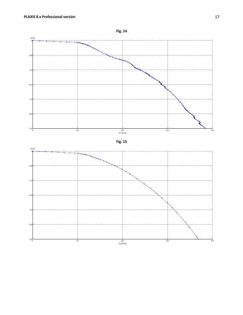
PLAXIS 8.x Professional version
17
Fig. 14
Fig. 15
0 2e3 4e3 6e3 8e3-0.3
-0.25
-0.2
-0.15
-0.1
-0.05
0
Fy [kN/rad]
Uy [m]
0 2e3 4e3 6e3 8e3-0.3
-0.25
-0.2
-0.15
-0.1
-0.05
0
Fy [kN/rad]
Uy [m]
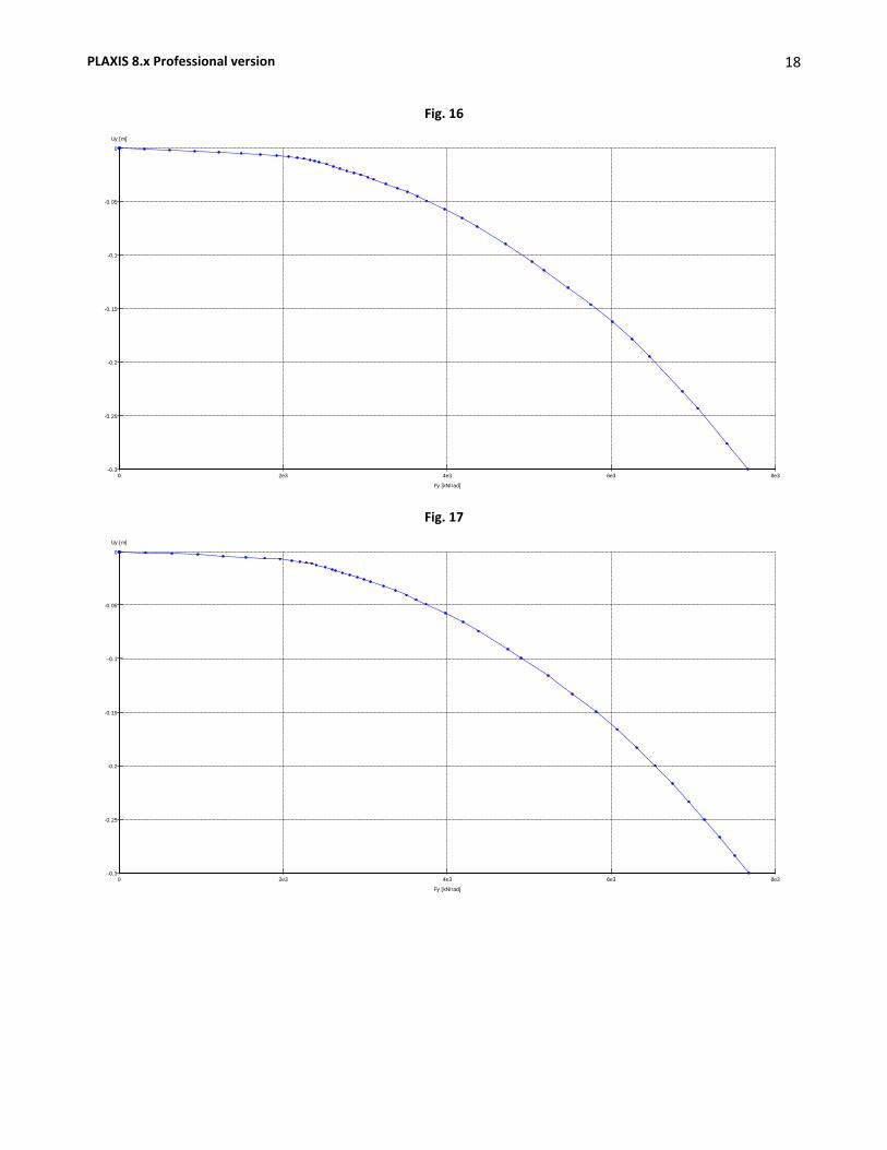
PLAXIS 8.x Professional version
18
Fig. 16
Fig. 17
0 2e3 4e3 6e3 8e3-0.3
-0.25
-0.2
-0.15
-0.1
-0.05
0
Fy [kN/rad]
Uy [m]
0 2e3 4e3 6e3 8e3-0.3
-0.25
-0.2
-0.15
-0.1
-0.05
0
Fy [kN/rad]
Uy [m]
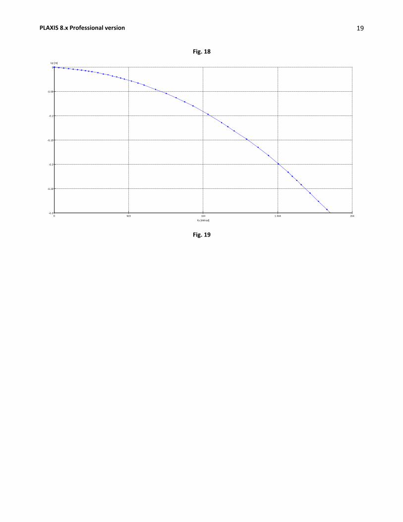
PLAXIS 8.x Professional version
19
Fig. 18
Fig. 19
0 5e3 1e4 1.5e4 2e4-0.3
-0.25
-0.2
-0.15
-0.1
-0.05
0
Fy [kN/rad]
Uy [m]
81
Appendix [2] – List of Published Papers
1. Nabil, M. and Abu Tair, A. (2017). Comparison Between Theoretical and Practical
Compression Capacities of Deep / Long Piles in Dubai. In: 3rd International Sustainable
Buildings Symposium (ISBS 2017).
2. Nabil, M. and Abu Tair, A. (2017). Comparison Between Theoretical and Practical
Compression Capacities of Deep / Long Piles in Dubai. In: 6th International Conference on
Geological and Environmental Sciences.
3. Nabil, M. and Abu Tair, A. (2017). Comparison Between Theoretical and Practical
Compression Capacities of Deep / Long Piles in Dubai. International Journal of Structural
and Civil Engineering Research, (E0002).
4. Nabil, M. and Abu Tair, A. (2017). Comparison Between Theoretical and Practical
Compression Capacities of Deep / Long Piles in Dubai. Springer, Proceedings of 3rd
International Sustainable Buildings Symposium. lSBS 2017(86924797).