bypass impulse problem - xsystem ltdaoct 04, 2015 · to help us “guess” at what kind of load...
TRANSCRIPT

1© Intergraph 2015
10/6/2015
© Intergraph 2015
A By-Pass Line Impulse Problem
Using CAESAR II asa Forensic Tool
© Intergraph 2015
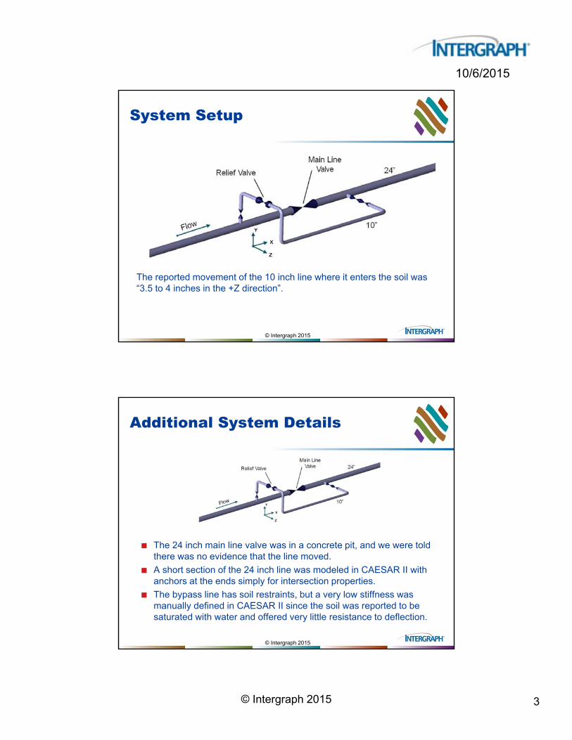
System Setup
A motor-operated main line valve on a 24 inch diameter oil transmission line closed and created a pressure rise on the upstream side of the valve, from approximately 1900 kPa to 3650 kPa (275 psi to 530 psi).

2© Intergraph 2015
10/6/2015
© Intergraph 2015
System Setup
The main line was protected from over-pressure by a 10 inch bypass line with a 12 inch in-line safety relief valve, designed to limit the pressure in the main line by discharging fluid back into the pipeline downstream of the main line valve.
© Intergraph 2015
System Setup
The relief valve successfully limited the pressure surge, but the opening of the relief valve caused a large lateral movement of the 10 inch bypass line, causing failure of some 3/8 inch instrumentation tubing, which resulted in the spilling of fluid.
3© Intergraph 2015
10/6/2015
© Intergraph 2015
System Setup
The reported movement of the 10 inch line where it enters the soil was “3.5 to 4 inches in the +Z direction”.
© Intergraph 2015
Additional System Details
The 24 inch main line valve was in a concrete pit, and we were told there was no evidence that the line moved.
A short section of the 24 inch line was modeled in CAESAR II with anchors at the ends simply for intersection properties.
The bypass line has soil restraints, but a very low stiffness was manually defined in CAESAR II since the soil was reported to be saturated with water and offered very little resistance to deflection.

4© Intergraph 2015
10/6/2015
© Intergraph 2015
Client Concerns/Questions
1. What caused this 3.5 to 4 inches of movement?
2. What can be done to prevent this problem from reoccurring?
Relief valve and instrumentation enclosure.
© Intergraph 2015
Possible Causes of this Event
1. What is the loading necessary to cause this event?
2. Could this be an unbalanced pressure load?
3. Could this be a slug load from momentum changes?
4. Could the event be a combination of both pressure and slug loads?
The fact that there was movement of the line indicates a dynamic load; presumably an impulse type of load.

5© Intergraph 2015
10/6/2015
© Intergraph 2015
An Issue with the Change in Pressure Approach
1. The reported direction of movement (+Z) is opposite to the unbalanced P•A load when the valve is opened.
2. Before the valve opens there are equal & opposite P•A loads on the valve and elbow. Upon valve opening, the P•A load is suddenly applied at the elbow.
3. Let’s ignore this “wrong direction” of movement for the moment.
© Intergraph 2015
Change in Momentum (Slug Load)
To see the system response to this (applied) slug load at node 130, we can perform a dynamic analysis.
But for a quick check, we can evaluate a static load equal to the induced load.
The maximum DLF for a one-time impulse load is 2.
Apply a static force of 2•345 = 690 lbf in the +Z direction at node 130 to see if we get something on the order of 3.5 inches of movement.

6© Intergraph 2015
10/6/2015
© Intergraph 2015
Forensic Analysis (slug)
Input Load Definition Load Case Setup
© Intergraph 2015
Forensic Analysis (slug)
Input Load Definition Load Case Setup
Results show a Z displacement of only 0.08 inches at node 130. Change in momentum, alone, cannot account for the observed field behavior.
7© Intergraph 2015
10/6/2015
© Intergraph 2015
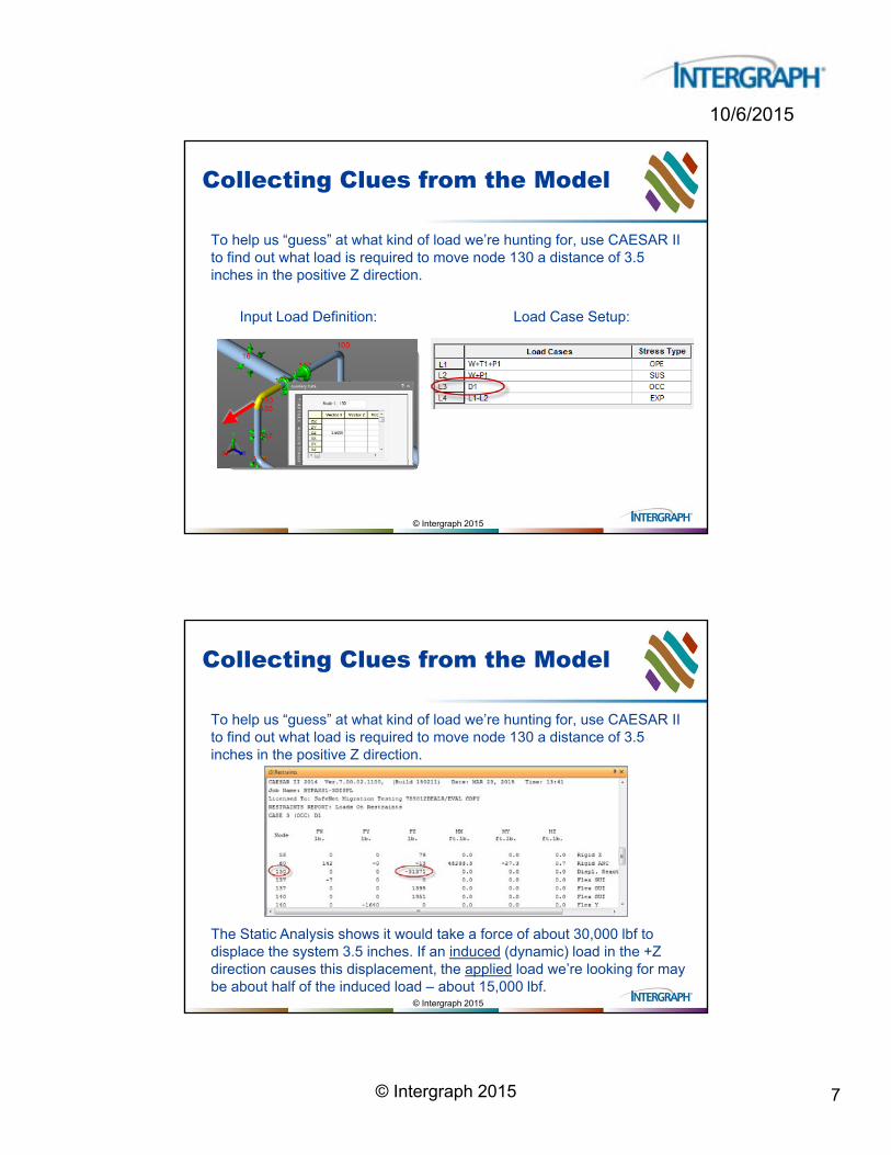
Collecting Clues from the Model
To help us “guess” at what kind of load we’re hunting for, use CAESAR II to find out what load is required to move node 130 a distance of 3.5 inches in the positive Z direction.
Input Load Definition: Load Case Setup:
© Intergraph 2015
Collecting Clues from the Model
To help us “guess” at what kind of load we’re hunting for, use CAESAR II to find out what load is required to move node 130 a distance of 3.5 inches in the positive Z direction.
The Static Analysis shows it would take a force of about 30,000 lbf to displace the system 3.5 inches. If an induced (dynamic) load in the +Z direction causes this displacement, the applied load we’re looking for may be about half of the induced load – about 15,000 lbf.

8© Intergraph 2015
10/6/2015
© Intergraph 2015
Searching for the Proper Load
The 345 lbf slug load is not significant enough to produce this behavior.
Let’s assume an applied thrust load due to the P•A effect. P = 3650 kPa = 529.5 psi
A = π/4•(OD-2t)2
OD = 10.75 in
t = 0.365 in
A = 78.85 in2
P•A = 529.5•78.85 = 41750 lbf
If the induced load is twice the applied load, the induced load may be as high as 83,500 lbf!
Neither change in momentum (slug), nor the pressure differential (P•A) can account for desired applied load of 15,000 lbf.
© Intergraph 2015
Forensic Analysis –evaluating the dynamic response
The induced load need not be twice the applied load. So the pressure thrust may be the cause
(We still have the “problem” with the discrepancy between thrust load direction and the system response.)
Let’s see what happens when we apply a P•A load.
It is reasonable to ignore the slug loading (even though it does exist), as the magnitude of the slug load is very small compared to the P•A load.
9© Intergraph 2015
10/6/2015
© Intergraph 2015
Forensic Analysis (ΔP)
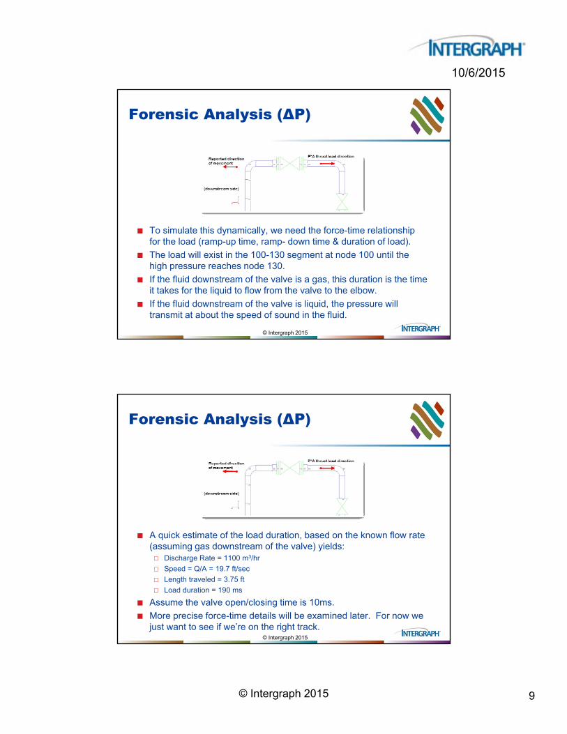
To simulate this dynamically, we need the force-time relationship for the load (ramp-up time, ramp- down time & duration of load).
The load will exist in the 100-130 segment at node 100 until the high pressure reaches node 130.
If the fluid downstream of the valve is a gas, this duration is the time it takes for the liquid to flow from the valve to the elbow.
If the fluid downstream of the valve is liquid, the pressure will transmit at about the speed of sound in the fluid.
© Intergraph 2015
Forensic Analysis (ΔP)
A quick estimate of the load duration, based on the known flow rate (assuming gas downstream of the valve) yields: Discharge Rate = 1100 m3/hr
Speed = Q/A = 19.7 ft/sec
Length traveled = 3.75 ft
Load duration = 190 ms
Assume the valve open/closing time is 10ms.
More precise force-time details will be examined later. For now we just want to see if we’re on the right track.
10© Intergraph 2015
10/6/2015
© Intergraph 2015
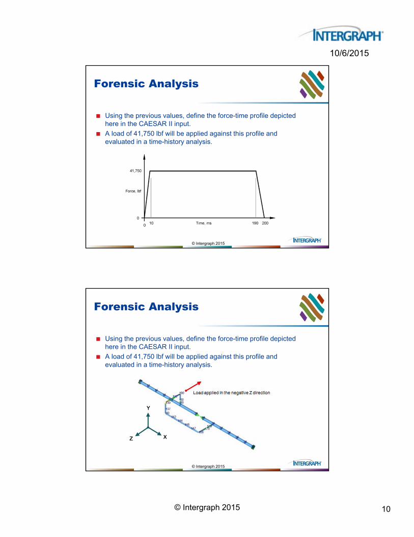
Forensic Analysis
Using the previous values, define the force-time profile depicted here in the CAESAR II input.
A load of 41,750 lbf will be applied against this profile and evaluated in a time-history analysis.
© Intergraph 2015
Forensic Analysis
Using the previous values, define the force-time profile depicted here in the CAESAR II input.
A load of 41,750 lbf will be applied against this profile and evaluated in a time-history analysis.
11© Intergraph 2015
10/6/2015
© Intergraph 2015
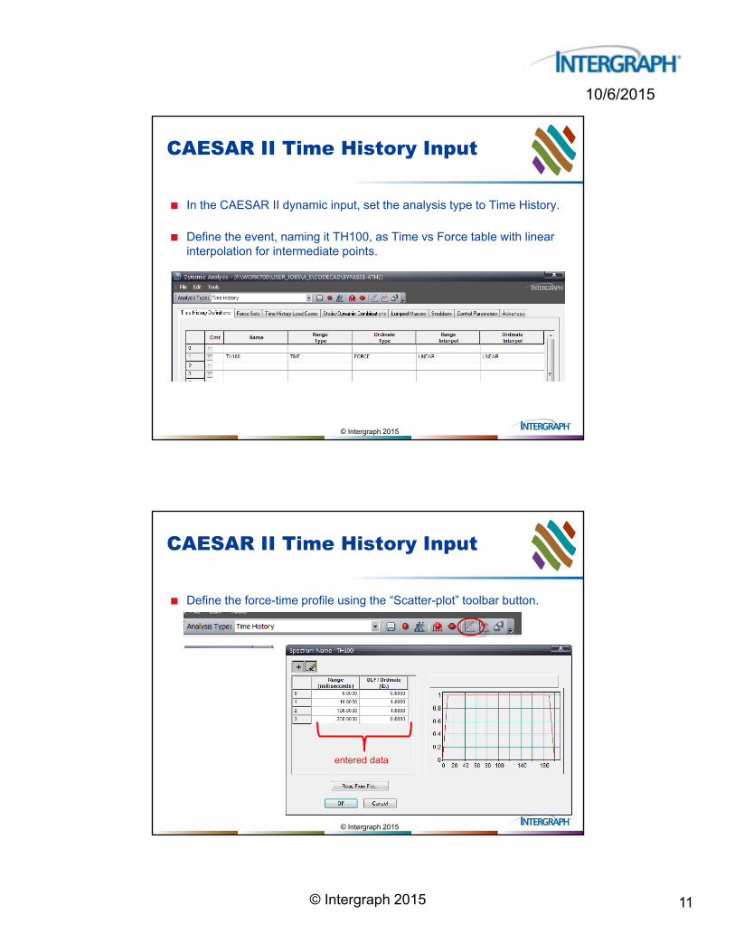
CAESAR II Time History Input
In the CAESAR II dynamic input, set the analysis type to Time History.
Define the event, naming it TH100, as Time vs Force table with linear interpolation for intermediate points.
© Intergraph 2015
CAESAR II Time History Input
Define the force-time profile using the “Scatter-plot” toolbar button.
entered data

12© Intergraph 2015
10/6/2015
© Intergraph 2015
CAESAR II Time History Input
Define the applied load: force magnitude, direction, location and label the force set beginning with 1.
Note the force magnitude (and direction) are defined here, not in the earlier definition of the pulse.
© Intergraph 2015
CAESAR II Time History Input
Build the time-history load case by combining the profile and the force set.
If a Code Stress evaluation is required, use the next tab to register the necessary Static/Dynamic Combination of (static) sustained stress with the occasional stress calculated here.

13© Intergraph 2015
10/6/2015
© Intergraph 2015
CAESAR II Time History Input
Lastly the Control Parameters must be set. It is essential to change the time-history time step and load duration values from their default. Typical values for this type of loading would be a time-history time step of 1 ms to 3 ms and a load duration of 0.5 to 1.0 seconds.
© Intergraph 2015
CAESAR II Time History Results
Run the analysis and review the output.
What does the generated displacement report show?
• Max DY exceeds 9 inches.
• Max DZ is -8.5 inches, the wrong way (compared to the field)!
14© Intergraph 2015
10/6/2015
© Intergraph 2015
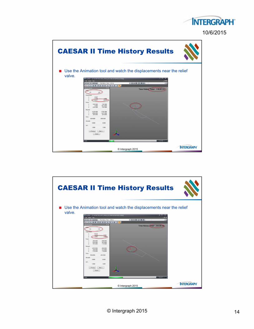
CAESAR II Time History Results
Use the Animation tool and watch the displacements near the relief valve.
© Intergraph 2015
CAESAR II Time History Results
Use the Animation tool and watch the displacements near the relief valve.

15© Intergraph 2015
10/6/2015
© Intergraph 2015
CAESAR II Time History Results
Use the Animation tool and watch the displacements near the relief valve.
The animation matches the text reports, but gives a better idea as to how the system is moving under this assumed load.
The system moves in -Z 8.5 inches (unreported), then bounces back to +Z 4 inches (reported).
© Intergraph 2015
Confirming the Model
The client (owner) was questioned about this numerical result, and whether the deflection in -Z (8.5 inches) made sense.
The client’s response was:
“Oh, that explains it!”. Explains what? He said that the long black cable on the left side of the photo used to be straight down to the pipe, and it ripped off during the event, which would require about 8” of movement. All of a sudden, everything made sense.
minus Z
16© Intergraph 2015
10/6/2015
© Intergraph 2015
Refining the Model
The timing assumptions used so far may be adequate, as the results match what was observed, and we perhaps can take aim at possible solutions.
Perhaps investigate the effects of the valve-opening time, and give some thought to what’s happening in the line, to get a more accurate force profile.
The results of this investigation might uncover more information which may be important when evaluating possible solutions.
© Intergraph 2015
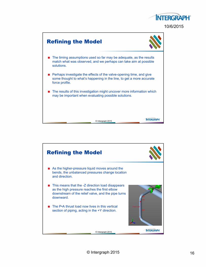
Refining the Model
As the higher-pressure liquid moves around the bends, the unbalanced pressures change location and direction.
This means that the -Z direction load disappears as the high pressure reaches the first elbow downstream of the relief valve, and the pipe turns downward.
The P•A thrust load now lives in this vertical section of piping, acting in the +Y direction.
17© Intergraph 2015
10/6/2015
© Intergraph 2015
Refining the Model
As the liquid begins to travel past the relief valve, the gas downstream compresses until the pressure is high enough upstream of the check valve to open it.
This changing pressure in the gas will influence the pressure differential between elbows, and the speed of the liquid flow.
© Intergraph 2015
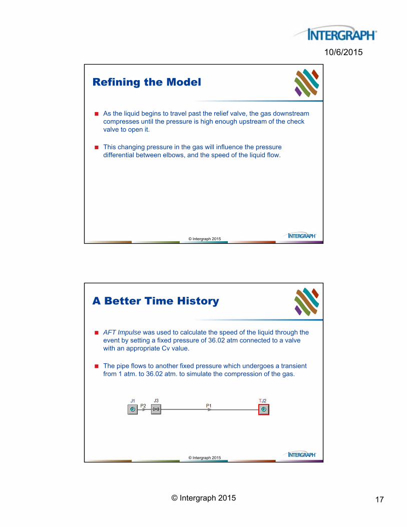
A Better Time History
AFT Impulse was used to calculate the speed of the liquid through the event by setting a fixed pressure of 36.02 atm connected to a valve with an appropriate Cv value.
The pipe flows to another fixed pressure which undergoes a transient from 1 atm. to 36.02 atm. to simulate the compression of the gas.

18© Intergraph 2015
10/6/2015
© Intergraph 2015
A Better Time History
AFT yields the pressure and flow velocity in each leg of the system.
© Intergraph 2015
A Better Time History
From this information, the force-time profiles for each leg of the by-pass line can be developed.

19© Intergraph 2015
10/6/2015
© Intergraph 2015
Updating the Event Time History
Add two more pulse definitions to the CAESAR II dynamic input.
© Intergraph 2015
Updating the Event Time History
Revise the first pulse, and add the data for the two new pulses.
20© Intergraph 2015
10/6/2015
© Intergraph 2015
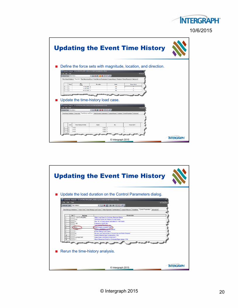
Updating the Event Time History
Define the force sets with magnitude, location, and direction.
Update the time-history load case.
© Intergraph 2015
Updating the Event Time History
Update the load duration on the Control Parameters dialog.
Rerun the time-history analysis.

21© Intergraph 2015
10/6/2015
© Intergraph 2015
Reviewing the Refined Results
Displacement data from the Animation Module.
DZ varies from +4.5 to -7.8 inches.
DY exceeds +21 inches!
DX exceeds -10 inches!
© Intergraph 2015
Checking the Results
Additional information from the owner in the form of a picture.
Note the trench in the X and Z directions. Here is more agreement between the analysis and the field!

22© Intergraph 2015
10/6/2015
© Intergraph 2015
How Do We Prevent This Response?
Solutions ?
Ideas?
© Intergraph 2015
How Do We Prevent This Response?
Solution1:
Slow the opening of the relief valve.
This doesn’t appear to be an option.
Some fear this would destroy the valve.
Reject this idea!

23© Intergraph 2015
10/6/2015
© Intergraph 2015
How Do We Prevent This Response?
Solution 2:
Replace the relief valve with a Control valve, that is opened slowly when the main valve starts to close.
The pressure-time data showed that the main valve closed 1.5 minutes before the relief valve opened. This gives adequate time to mitigate the problem with a different type of valve.
© Intergraph 2015
How Do We Prevent This Response?
Solution 3:
Add a restraint to change the system response and absorb the load.
The equivalent load is on the order of 84,000 lb, a restraint could be expensive.
Better ideas are to either not respond to the load or eliminate the load (if possible).

24© Intergraph 2015
10/6/2015
© Intergraph 2015
How Do We Prevent This Response?
Solution 4:
Ensure the by-pass line is filled with liquid.
This causes the pressure wave to transmit at the speed of sound in the liquid.
This reduces the response to something manageable because of the extremely short load durations.
© Intergraph 2015
How Do We Prevent This Response?
Solution 5:
Replace the relief valve with a manual valve that is “chained” open. This avoids accidental closure.
If the valve must be closed, it is a conscious, manual process.
25© Intergraph 2015
10/6/2015
© Intergraph 2015
By-Pass Line Impulse Problem
Questions ?
Comments?
© Intergraph 2015
By-Pass Line Impulse Problem
Thank You