f=kx - xsystem ltda · pdf file01.10.2015 · caesar ii caux 2015 3/23/2015 2 math...
TRANSCRIPT
CAESAR II CAUx 2015 3/23/2015
1
© Intergraph 2015
F=KX
How CAESAR II formulates the global stiffness matrix
© Intergraph 2015
Agenda
Math basics
Comparing matrix math to CAESAR II Single pipe element
Single bend
A two pipe system
A pipe-bend-pipe system
A tee
Other considerations
Content developed as part of the CAESAR II on-line video training series.

CAESAR II CAUx 2015 3/23/2015
2
MATH BASICSTo the guided cantilever method
© Intergraph 2015
Concept
What is the thermal load on single pipe between two anchors? 4 inch schedule STD
Temperature = 350°C
Length undefined (L)

CAESAR II CAUx 2015 3/23/2015
3
© Intergraph 2015
Approach
What is the thermal load on single pipe between two anchors? 4 inch schedule STD
Temperature = 350°C
Length undefined (L)
Determine free thermal growth: ∆=αL
∆
© Intergraph 2015
Approach
What is the thermal load on single pipe between two anchors? 4 inch schedule STD
Temperature = 350°C
Length undefined (L)
Determine free thermal growth: ∆=αL
Calculate load to return the end: P=K ∆ ; K=AE/L
∆
CAESAR II CAUx 2015 3/23/2015
4
© Intergraph 2015
Math Basics
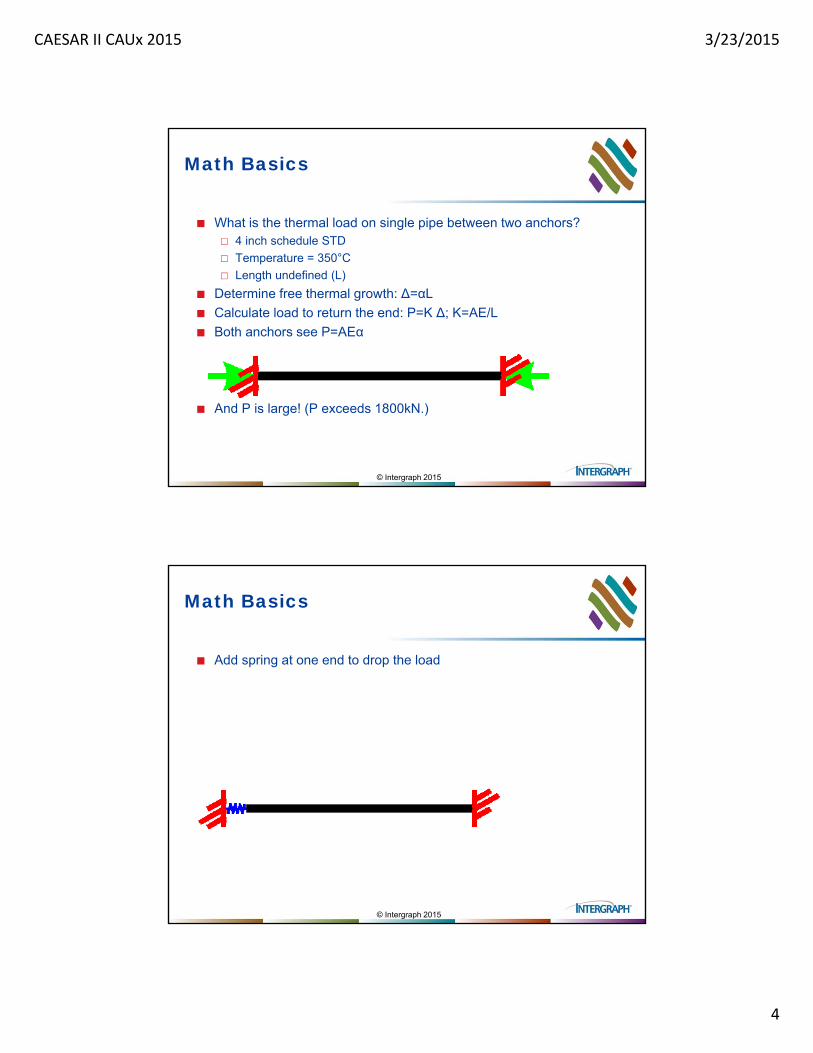
What is the thermal load on single pipe between two anchors? 4 inch schedule STD
Temperature = 350°C
Length undefined (L)
Determine free thermal growth: ∆=αL
Calculate load to return the end: P=K ∆; K=AE/L
Both anchors see P=AEα
And P is large! (P exceeds 1800kN.)
© Intergraph 2015
Math Basics
Add spring at one end to drop the load

CAESAR II CAUx 2015 3/23/2015
5
© Intergraph 2015
Math Basics
Add spring at one end to drop the load
Again, what is the load (P) required to return free growth?
Monitor two positions: δ, ∆ · Δ ·
· Δ
· · · Δ
∆δ
KS KP
© Intergraph 2015
Math Basics
· · · Δ If ≫ ; → 1 and · ∆ (our original result)
If ≫ ; → 1 and · ∆ (based solely on KS!)
You can dial in any load you wish by adjusting support stiffness!
∆δ
KS KP

CAESAR II CAUx 2015 3/23/2015
6
© Intergraph 2015
Math Basics
Yes, you can dial in any load you wish by adjusting support stiffness
But seldom is that an option.
What if that spring was replaced by a cantilever?
?
© Intergraph 2015
Math Basics
Cantilever stiffness is a function of the end conditions: Free end (rotation allowed):
Guided end (no rotation):
?
3 · ·
12 · ·
(Conservative)
12 · ·
Assume corner remains square
CAESAR II CAUx 2015 3/23/2015
7
© Intergraph 2015
Math Basics
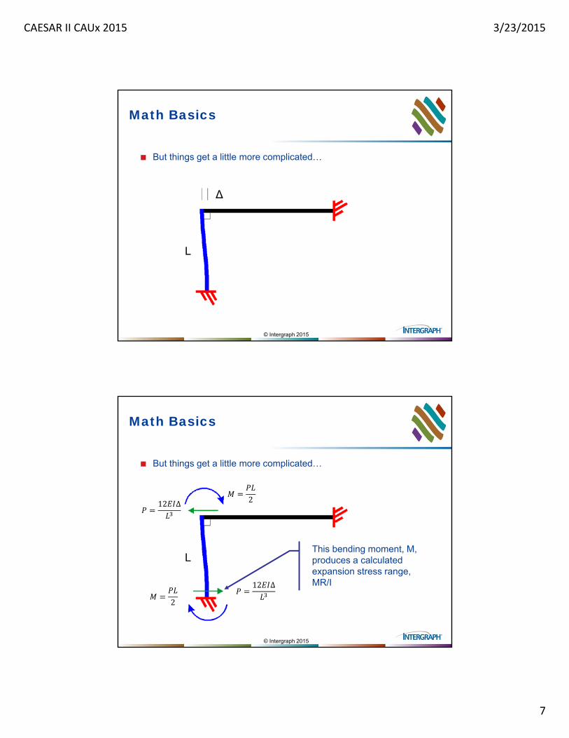
But things get a little more complicated…
∆
L
© Intergraph 2015
Math Basics
But things get a little more complicated…
L
12 ∆
2
12 ∆
2
This bending moment, M, produces a calculated expansion stress range, MR/I
CAESAR II CAUx 2015 3/23/2015
8
© Intergraph 2015
Math Basics
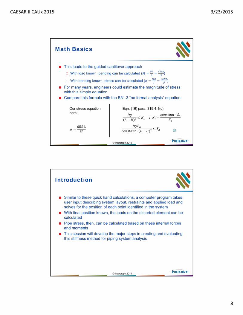
This leads to the guided cantilever approach
With load known, bending can be calculated (∆)
With bending known, stress can be calculated (∆)
For many years, engineers could estimate the magnitude of stress with this simple equation
Compare this formula with the B31.3 “no formal analysis” equation:
6 ∆·
; ·
Eqn. (16) para. 319.4.1(c):Our stress equation here:
© Intergraph 2015
Introduction
Similar to these quick hand calculations, a computer program takes user input describing system layout, restraints and applied load and solves for the position of each point identified in the system
With final position known, the loads on the distorted element can be calculated
Pipe stress, then, can be calculated based on these internal forces and moments
This session will develop the major steps in creating and evaluating this stiffness method for piping system analysis

CAESAR II CAUx 2015 3/23/2015
9
© Intergraph 2015
Flexibility Method – life before the PC
Beyond the guided cantilever method, larger systems were analyzed using the flexibility method The US Navy’s Mare Island program (MEC 21) was one of the first
CAESAR II still references the bend formula found in MEC 21
Flexibility Method – X=AF: position equals flexibility times load Direct solution – know A & F, find X
Piping codes continue to offer flexibility factor for elbows
Limited to static analysis
Dynamic solution works with stiffness (e.g. ⁄ ), not flexibility
Auton Computing’s conversion from Autoflex to Dynaflex in 1970’s
Stiffness Method – F=KX: load equals stiffness times position Know F & K, find X
n equations with n unknowns
COMPARING MATRIX MATH TO CAESAR II
A Series of Examples

CAESAR II CAUx 2015 3/23/2015
10
© Intergraph 2015
Session Format
Concepts in F=KX will first be developed.
These concepts will be expressed in Mathcad
Followed with a CAESAR II analysis.
Results will be compared.
To keep it simple, all models are planar (2-D) Rather than dealing with 6 degrees of freedom for every node, we will
be using X, Y & RZ
© Intergraph 2015
#1 The simple beam element (in 2-D)
Build and load the stiffness matrix for a single straight pipe Set stiffness terms in Mathcad
Build a 2D (planar) beam stiffness matrix for a 4”Std pipe
Add anchor at near end
Compare with CAESAR II Displace far end
Apply loads at far end
CAESAR II Models: 1 ELEMENT PLANAR1 ELEMENT PLANAR - FORCES

CAESAR II CAUx 2015 3/23/2015
11
© Intergraph 2015
#2 The bend element
Build and load a 2D bend element What is a flexibility factor
© Intergraph 2015
What of this Flexibility Factor?
Except for elbows, bends and miters, the component flexibility factor is 1.
For an elbow this factor is 1.65/h:
CAESAR II CAUx 2015 3/23/2015
12
© Intergraph 2015
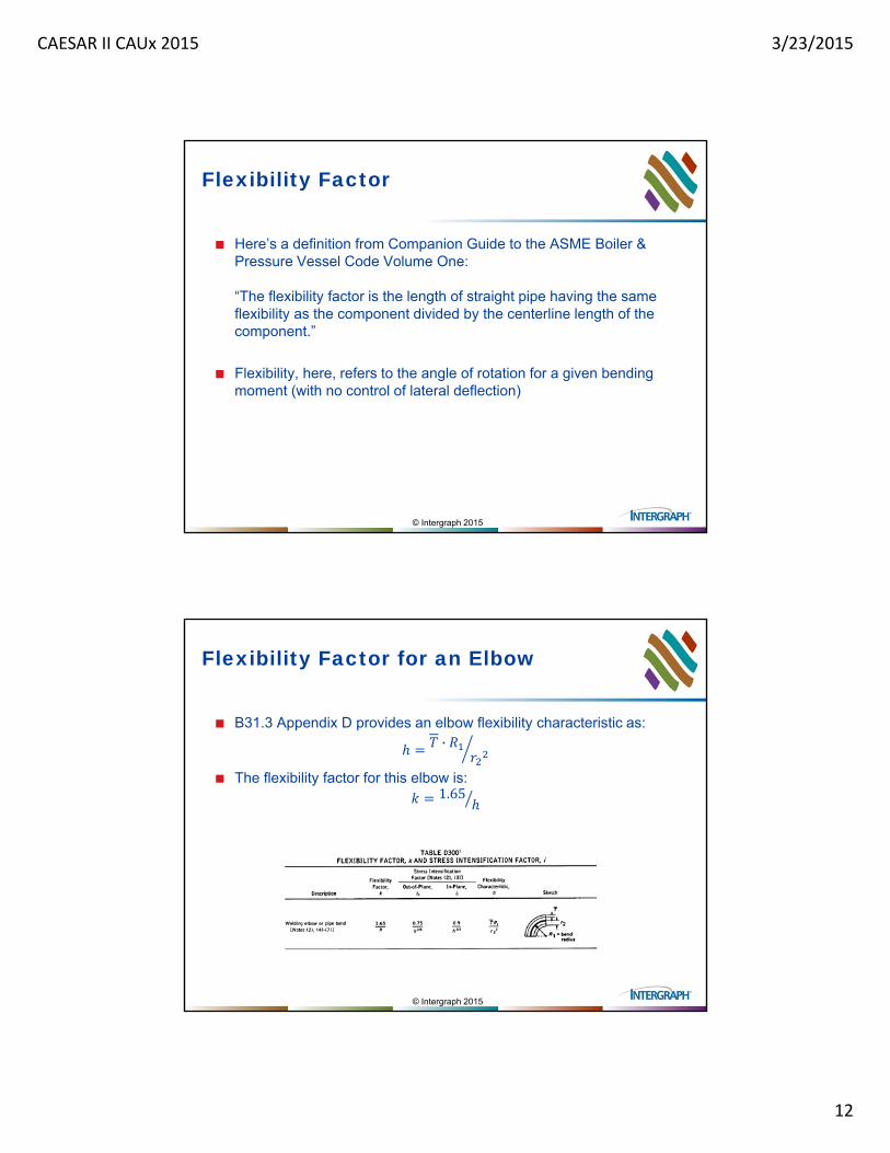
Flexibility Factor
Here’s a definition from Companion Guide to the ASME Boiler & Pressure Vessel Code Volume One:
“The flexibility factor is the length of straight pipe having the same flexibility as the component divided by the centerline length of the component.”
Flexibility, here, refers to the angle of rotation for a given bending moment (with no control of lateral deflection)
© Intergraph 2015
Flexibility Factor for an Elbow
B31.3 Appendix D provides an elbow flexibility characteristic as:·
The flexibility factor for this elbow is:1.65

CAESAR II CAUx 2015 3/23/2015
13
© Intergraph 2015
Flexibility Factor Example
A 4 inch, standard wall, long radius elbow will have the following terms:
6.0198 , 152.4 , 54.14 Therefore flexibility factor for this elbow is:
5.272 The arc length of this elbow is:
L 2 · 239.4
So a straight pipe that is · 1262 long should have the same end rotation as this elbow.
© Intergraph 2015
Flexibility Factor Example
A 4”STD straight pipe that is 1262mm long should have the same end rotation as its long radius elbow:
1262
Q.E.D.
CAESAR II Model: FLEX CHECK

CAESAR II CAUx 2015 3/23/2015
14
© Intergraph 2015
The bend element
Build and load a 2D bend element Build a (local) flexibility matrix
Check flexibility matrix in CAESAR II
Generate a stiffness matrix from the flexibility matrix
Add anchor
Compare with CAESAR II Displace far end (F=KX)
Apply loads on far end (X=AF)
CAESAR II Model: BEND
© Intergraph 2015
The bend element
Build and load a 2D bend element Build a (local) flexibility matrix
Check flexibility matrix in CAESAR II
Generate a stiffness matrix from the flexibility matrix
Add anchor
Compare with CAESAR II Displace far end (F=KX)
Apply loads on far end (X=AF)
Other discussion
B31.3 Appx. D provides an adjustment for stiffeners (flanges) that restrict ovalization
CAESAR II provides a scratchpad to review these values
CAESAR II CAUx 2015 3/23/2015
15
© Intergraph 2015
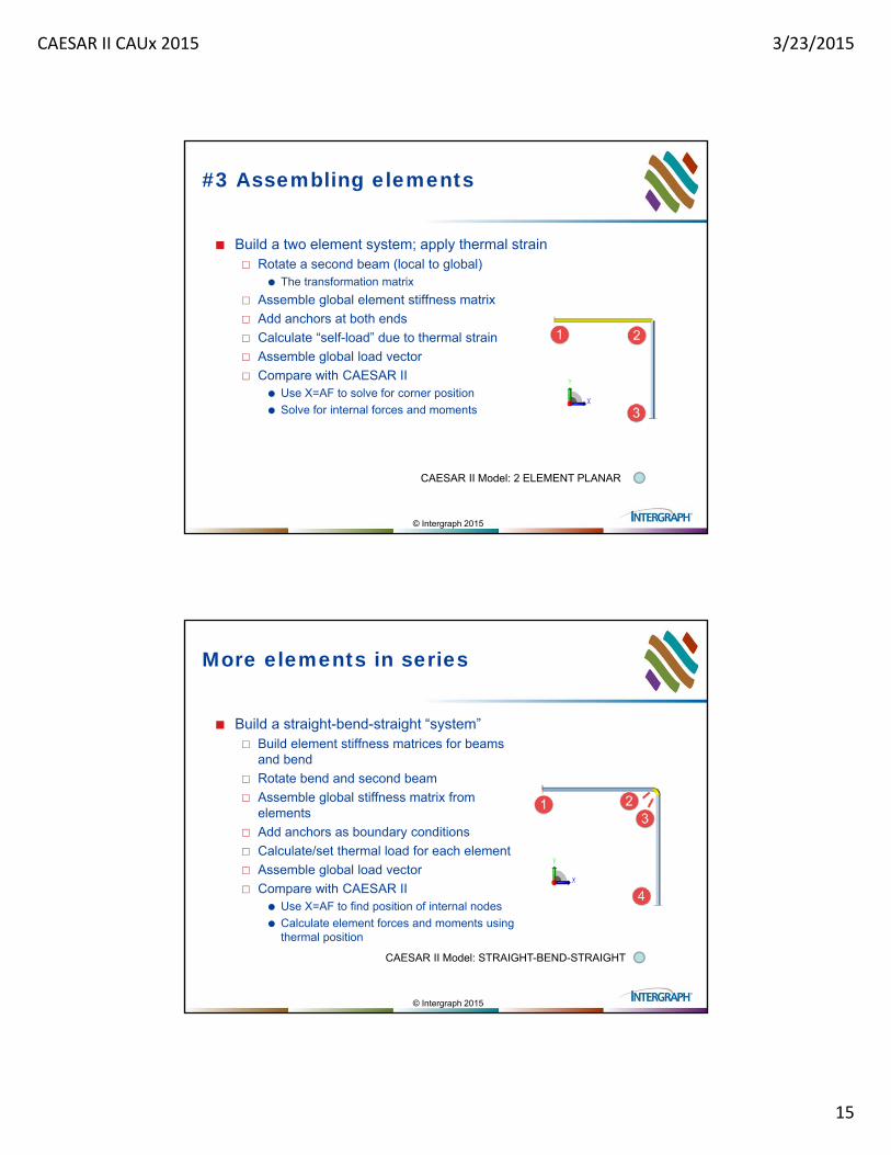
#3 Assembling elements
Build a two element system; apply thermal strain Rotate a second beam (local to global)
The transformation matrix
Assemble global element stiffness matrix
Add anchors at both ends
Calculate “self-load” due to thermal strain
Assemble global load vector
Compare with CAESAR II Use X=AF to solve for corner position
Solve for internal forces and moments
CAESAR II Model: 2 ELEMENT PLANAR
© Intergraph 2015
More elements in series
Build a straight-bend-straight “system” Build element stiffness matrices for beams
and bend
Rotate bend and second beam
Assemble global stiffness matrix from elements
Add anchors as boundary conditions
Calculate/set thermal load for each element
Assemble global load vector
Compare with CAESAR II Use X=AF to find position of internal nodes
Calculate element forces and moments using thermal position
CAESAR II Model: STRAIGHT-BEND-STRAIGHT

CAESAR II CAUx 2015 3/23/2015
16
© Intergraph 2015
#4 Branches
CAESAR II Model: TEE
Build a branched “system” Build local stiffness matrices for beams
Rotate run pipe to global system
Assemble stiffness matrix from elements –focus on offset applied to branch
Add boundary conditions (anchors and restraint)
Calculate/set thermal load for each element
Build load vector – offset vector position
Compare with CAESAR II Use X=AF to find position of internal nodes
Calculate element forces and moments using thermal position
Other points Bandwidth
OTHER CONSIDERATIONS
CAESAR II CAUx 2015 3/23/2015
17
© Intergraph 2015
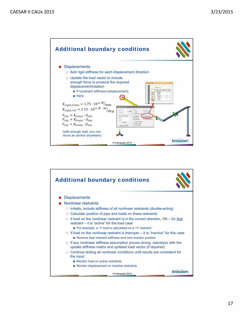
Additional boundary conditions
Displacements Add rigid stiffness for each displacement direction
Update the load vector to include enough force to produce the required displacement/rotation F=(restraint stiffness)*(displacement)
Here:
_ 1.75 · 10
_ 1.13 · 10 ·
···
(with enough load, you can move an anchor anywhere)
© Intergraph 2015
Additional boundary conditions
Displacements
Nonlinear restraints Initially, include stiffness of all nonlinear restraints (double-acting)
Calculate position of pipe and loads on these restraints
If load on the nonlinear restraint is in the correct direction, OK – for thatrestraint – it is “active” for the load case For example, a -Y load is calculated on a +Y restraint
If load on the nonlinear restraint is improper – it is “inactive” for this case Remove that restraint stiffness and now monitor position
If any nonlinear stiffness assumption proves wrong, reanalyze with the update stiffness matrix and updated load vector (if required)
Continue testing all nonlinear conditions until results are consistent for the input: Monitor load on active restraints
Monitor displacement on inactive restraints

CAESAR II CAUx 2015 3/23/2015
18
© Intergraph 2015
Additional boundary conditions
Displacements
Nonlinear restraints
Friction (stick/slip) Initial condition (assume stick) – Add translational restraints
perpendicular to the restraint vector with coefficient of friction (μ) specified
If restraint load on that pair of added restraints is less than the resisting force, μN, model is valid
If restraint load on that pair of added restraints is greater than the resisting force, μN, model is updated – remove restraints and provide a friction force, μN, opposite the vector loading those remove restraints
© Intergraph 2015
Additional boundary conditions
Displacements
Nonlinear restraints
Friction (stick/slip)
CNodes Consider as a “partial” element with connection based on restraint type
For example: Matrix at right shows the planar (X,Y,RZ)
stiffness matrix for a 4 node system
If Node 1 was rigidly connected to Node 4 in the X direction, then
Add rigid stiffness in X between 1 & 4
(Other cells in 1:4 and 4:1 remain empty)

CAESAR II CAUx 2015 3/23/2015
19
© Intergraph 2015
A note on load vectors
Primitive loads are used to build CAESAR II load cases
Each primitive provides a load vector component
Load cases combine these primitive loads
For example: Load Case 1: W+P1+T1+D1 (OPE) Individual load vectors are assembled
(here, w1 is the x,y,z,rx,ry,rz weight load assigned to node 1)
The load vector used with the global stiffness matrix, then, is:
Solve for X in F=KX
or
© Intergraph 2015
Flexibility at branch connections
STP-PT-073: Stress Intensity Factor and k-Factor Alignment for Metallic Pipes Table 1 – Flexibility and Stress Intensification Factors (Sketch No. 2+)
Nonmandatory Appendix D – Calculating Flexibility Factors for Branch Connection Models in Piping Systems

CAESAR II CAUx 2015 3/23/2015
20
© Intergraph 2015
Flexibility at branch connections
STP-PT-073: Stress Intensity Factor and k-Factor Alignment for Metallic Pipes
FEATools
F=KX AS APPLIED IN CAESAR IIQuestions / Comments
CAESAR II CAUx 2015 3/23/2015
21
© Intergraph 2015
More Information…
Again, this content was initially developed as part of the CAESAR II on-line video training series. (Visit www.pipingdesignonline.com)
Along with the (captioned) videos, there is a workbook for the many exercises.
F=KX AS APPLIED IN CAESAR IIThank you