c 2010 ajit rajwade - university of...
TRANSCRIPT

PROBABILISTIC APPROACHES TO IMAGE REGISTRATION AND DENOISING
By
AJIT RAJWADE
A DISSERTATION PRESENTED TO THE GRADUATE SCHOOLOF THE UNIVERSITY OF FLORIDA IN PARTIAL FULFILLMENT
OF THE REQUIREMENTS FOR THE DEGREE OFDOCTOR OF PHILOSOPHY
UNIVERSITY OF FLORIDA
2010

c© 2010 Ajit Rajwade
2

This thesis is being submitted with a feeling of gratitude for my parents and brother,
whom I consider to be my best and closest friends.
3

ACKNOWLEDGMENTS
I would like to thank my advisors Dr. Anand Rangarajan and Dr. Arunava Banerjee
for sharing with me their endless enthusiasm, knowledge, expertise and love for the
subject. I have come to admire not only their intellect but also their unassuming and
informal nature. They treat their students like friends! Anand and Arunava are two
individuals who are full of ideas, and who are willing to selflessly share those ideas with
everybody. I am indebted to them for having given me the freedom to pursue towards
my Ph.D. a problem that I was passionate about, namely image denoising. I am also
thankful to both of them for having played a big role in encouraging student-student
collaborations on research problems of mutual interest. Such open-mindedness and
enthusiasm is rare!
I would like to thank Dr. Jeffrey Ho, Dr. Baba Vemuri and Dr. Brett Presnell for
serving on my committee. I deeply appreciate Dr. Presnell’s efforts in reading my thesis
and suggesting me useful changes, and for discussions on probability density estimation
techniques. A word of sincere appreciation for several faculty members from the CISE
department: Dr. Alper Ungor, Dr. Sanjay Ranka, Dr. Pete Dobbins, Dr. Paul Gader
and Dr. Tim Davis, with whom I have worked as teaching assistant; and for Dr. Meera
Sitharam, with whom I participated in our local chapter of SPICMACAY, an organization
for promotion of Indian classical music.
Gainesville would have been a boring place without my room-mates and lab-mates:
Venkatakrishnan Ramaswamy, Subhajit Sengupta, Karthik Gurumoorthy, Bhupinder
Singh, Amit Dhurandhar, Gnana Sundar Rajendiran, Milapjit Sandhu, Ravneet
Singh Vohra, Sayan Banerjee, Alok Whig, Meizhu Liu, Ting Chen, Guang Chung,
Angelos Barmpoutis, Ritwik Kumar, Fei Wang, Bing Jian, Santhosh Kodipaka, Esen
Yuksel, Wenxing Ye, Yuchen Xie, Dohyung Seo, Sile Hu, Jason Chi, Shahed Nejhum,
Manu Sethi, Mohsen Ali, Adrian Peter, Neil Smith, Karthik Gopalkrishnan, Srikanth
Subramaniam, and many others. They all helped build a lively environment both at
4

home and in the lab. I consider myself lucky to have had two really wonderful friends:
Venkatakrishnan Ramaswamy (here at UF) and Gurman Singh Gill (at McGill), who have
been such genuine well-wishers all along! I have also come to admire Venkat’s ability to
ask (innumerable :-)) interesting questions on matters both technical and non-technical.
No words can be sufficient to thank my parents, my brother and my grandparents
who never let me feel that I was alone on this long, challenging and sometimes
frustrating journey. This thesis would have been impossible without their support. I
wish to express my sincerest gratitude to the Saswadkar and Iyengar families back
in Pune, who have been friends, philosphers and guides for my family, and who have
helped and supported us in just so many, many priceless ways!
5
TABLE OF CONTENTS
page
ACKNOWLEDGMENTS . . . . . . . . . . . . . . . . . . . . . . . . . . . . . . . . . . 4
LIST OF TABLES . . . . . . . . . . . . . . . . . . . . . . . . . . . . . . . . . . . . . . 10
LIST OF FIGURES . . . . . . . . . . . . . . . . . . . . . . . . . . . . . . . . . . . . . 12
ABSTRACT . . . . . . . . . . . . . . . . . . . . . . . . . . . . . . . . . . . . . . . . . 16
CHAPTER
1 INTRODUCTION . . . . . . . . . . . . . . . . . . . . . . . . . . . . . . . . . . . 18
2 PROBABILITY DENSITY WITH ISOCONTOURS AND ISOSURFACES . . . . 21
2.1 Overview of Existing PDF Estimators . . . . . . . . . . . . . . . . . . . . . 212.1.1 The Histogram Estimator . . . . . . . . . . . . . . . . . . . . . . . . 212.1.2 The Frequency Polygon . . . . . . . . . . . . . . . . . . . . . . . . 222.1.3 Kernel Density Estimators . . . . . . . . . . . . . . . . . . . . . . . 222.1.4 Mixture Models . . . . . . . . . . . . . . . . . . . . . . . . . . . . . 242.1.5 Wavelet-Based Density Estimators . . . . . . . . . . . . . . . . . . 25
2.2 Marginal and Joint Density Estimation . . . . . . . . . . . . . . . . . . . . 262.2.1 Estimating the Marginal Densities in 2D . . . . . . . . . . . . . . . 272.2.2 Related Work . . . . . . . . . . . . . . . . . . . . . . . . . . . . . . 292.2.3 Other Methods for Derivation . . . . . . . . . . . . . . . . . . . . . 292.2.4 Estimating the Joint Density . . . . . . . . . . . . . . . . . . . . . . 302.2.5 From Densities to Distributions . . . . . . . . . . . . . . . . . . . . 332.2.6 Joint Density between Multiple Images in 2D . . . . . . . . . . . . 352.2.7 Extensions to 3D . . . . . . . . . . . . . . . . . . . . . . . . . . . . 362.2.8 Implementation Details for the 3D case . . . . . . . . . . . . . . . . 382.2.9 Joint Densities by Counting Points and Measuring Lengths . . . . . 39
2.3 Experimental Results: Area-Based PDFs Versus Histograms with SeveralSub-Pixel Samples . . . . . . . . . . . . . . . . . . . . . . . . . . . . . . . 42
3 APPLICATION TO IMAGE REGISTRATION . . . . . . . . . . . . . . . . . . . . 50
3.1 Entropy Estimators in Image Registration . . . . . . . . . . . . . . . . . . 503.2 Image Entropy and Mutual Information . . . . . . . . . . . . . . . . . . . . 533.3 Experimental Results . . . . . . . . . . . . . . . . . . . . . . . . . . . . . 55
3.3.1 Registration of Two images in 2D . . . . . . . . . . . . . . . . . . . 553.3.2 Registration of Multiple Images in 2D . . . . . . . . . . . . . . . . . 583.3.3 Registration of Volume Datasets . . . . . . . . . . . . . . . . . . . 58
3.4 Discussion . . . . . . . . . . . . . . . . . . . . . . . . . . . . . . . . . . . 60
6

4 APPLICATION TO IMAGE FILTERING . . . . . . . . . . . . . . . . . . . . . . . 70
4.1 Introduction . . . . . . . . . . . . . . . . . . . . . . . . . . . . . . . . . . . 704.2 Theory . . . . . . . . . . . . . . . . . . . . . . . . . . . . . . . . . . . . . . 714.3 Extensions of Our Theory . . . . . . . . . . . . . . . . . . . . . . . . . . . 75
4.3.1 Color Images . . . . . . . . . . . . . . . . . . . . . . . . . . . . . . 754.3.2 Chromaticity Fields . . . . . . . . . . . . . . . . . . . . . . . . . . . 764.3.3 Gray-scale Video . . . . . . . . . . . . . . . . . . . . . . . . . . . . 77
4.4 Level Curve Based Filtering in a Mean Shift Framework . . . . . . . . . . 774.5 Experimental Results . . . . . . . . . . . . . . . . . . . . . . . . . . . . . 79
4.5.1 Gray-scale Images . . . . . . . . . . . . . . . . . . . . . . . . . . . 804.5.2 Testing on a Benchmark Dataset of Gray-scale Images . . . . . . . 804.5.3 Experiments with Color Images . . . . . . . . . . . . . . . . . . . . 814.5.4 Experiments with Chromaticity Vectors and Video . . . . . . . . . . 81
4.6 Discussion . . . . . . . . . . . . . . . . . . . . . . . . . . . . . . . . . . . 82
5 A RELATED PROBLEM: DIRECTIONAL STATISTICS IN EUCLIDEAN SPACE 95
5.1 Introduction . . . . . . . . . . . . . . . . . . . . . . . . . . . . . . . . . . . 955.2 Theory . . . . . . . . . . . . . . . . . . . . . . . . . . . . . . . . . . . . . . 96
5.2.1 Choice of Kernel . . . . . . . . . . . . . . . . . . . . . . . . . . . . 965.2.2 Using Random Variable Transformation . . . . . . . . . . . . . . . 975.2.3 Application to Kernel Density Estimation . . . . . . . . . . . . . . . 995.2.4 Mixture Models for Directional Data . . . . . . . . . . . . . . . . . . 1015.2.5 Properties of the Projected Normal Estimator . . . . . . . . . . . . 103
5.3 Estimation of the Probability Density of Hue . . . . . . . . . . . . . . . . . 1045.4 Discussion . . . . . . . . . . . . . . . . . . . . . . . . . . . . . . . . . . . 107
6 IMAGE DENOISING: A LITERATURE REVIEW . . . . . . . . . . . . . . . . . . 110
6.1 Introduction . . . . . . . . . . . . . . . . . . . . . . . . . . . . . . . . . . . 1106.2 Partial Differential Equations . . . . . . . . . . . . . . . . . . . . . . . . . 1116.3 Spatially Varying Convolution and Regression . . . . . . . . . . . . . . . . 1136.4 Transform-Domain Denoising . . . . . . . . . . . . . . . . . . . . . . . . . 116
6.4.1 Choice of Basis . . . . . . . . . . . . . . . . . . . . . . . . . . . . . 1176.4.2 Choice of Thresholding Scheme and Parameters . . . . . . . . . . 1186.4.3 Method for Aggregation of Overlapping Estimates . . . . . . . . . . 1196.4.4 Choice of Patch Size . . . . . . . . . . . . . . . . . . . . . . . . . . 119
6.5 Non-local Techniques . . . . . . . . . . . . . . . . . . . . . . . . . . . . . 1216.6 Use of Residuals in Image Denoising . . . . . . . . . . . . . . . . . . . . . 124
6.6.1 Constraints on Moments of the Residual . . . . . . . . . . . . . . . 1246.6.2 Adding Back Portions of the Residual . . . . . . . . . . . . . . . . . 1256.6.3 Use of Hypothesis Tests . . . . . . . . . . . . . . . . . . . . . . . . 1256.6.4 Residuals in Joint Restoration of Multiple Images . . . . . . . . . . 126
6.7 Denoising Techniques using Machine Learning . . . . . . . . . . . . . . . 1276.8 Common Problems with Contemporary Denoising Techniques . . . . . . . 129
7
6.8.1 Validation of Denoising Algorithms . . . . . . . . . . . . . . . . . . 1296.8.2 Automated Filter Parameter Selection . . . . . . . . . . . . . . . . 131
7 BUILDING UPON THE SINGULAR VALUE DECOMPOSITION FOR IMAGEDENOISING . . . . . . . . . . . . . . . . . . . . . . . . . . . . . . . . . . . . . 132
7.1 Introduction . . . . . . . . . . . . . . . . . . . . . . . . . . . . . . . . . . . 1327.2 Matrix SVD . . . . . . . . . . . . . . . . . . . . . . . . . . . . . . . . . . . 1337.3 SVD for Image Denoising . . . . . . . . . . . . . . . . . . . . . . . . . . . 1337.4 Oracle Denoiser with the SVD . . . . . . . . . . . . . . . . . . . . . . . . . 1347.5 SVD, DCT and Minimum Mean Squared Error Estimators . . . . . . . . . 136
7.5.1 MMSE Estimators with DCT . . . . . . . . . . . . . . . . . . . . . . 1367.5.2 MMSE Estimators with SVD . . . . . . . . . . . . . . . . . . . . . . 1387.5.3 Results with MMSE Estimators Using DCT . . . . . . . . . . . . . . 139
7.5.3.1 Synthetic patches . . . . . . . . . . . . . . . . . . . . . . 1397.5.3.2 Real images and a large patch database . . . . . . . . . 139
7.5.4 Results with MMSE Estimators Using SVD . . . . . . . . . . . . . . 1407.5.4.1 Synthetic patches . . . . . . . . . . . . . . . . . . . . . . 1407.5.4.2 Real images and a large patch database . . . . . . . . . 141
7.6 Filtering of SVD Bases . . . . . . . . . . . . . . . . . . . . . . . . . . . . . 1427.7 Nonlocal SVD with Ensembles of Similar Patches . . . . . . . . . . . . . . 143
7.7.1 Choice of Patch Similarity Measure . . . . . . . . . . . . . . . . . . 1477.7.2 Choice of Threshold for Truncation of Transform Coefficients . . . . 1497.7.3 Outline of NL-SVD Algorithm . . . . . . . . . . . . . . . . . . . . . 1507.7.4 Averaging of Hypotheses . . . . . . . . . . . . . . . . . . . . . . . 1507.7.5 Visualizing the Learned Bases . . . . . . . . . . . . . . . . . . . . 1507.7.6 Relationship with Fourier Bases . . . . . . . . . . . . . . . . . . . . 151
7.8 Experimental Results . . . . . . . . . . . . . . . . . . . . . . . . . . . . . 1527.8.1 Discussion of Results . . . . . . . . . . . . . . . . . . . . . . . . . 1537.8.2 Comparison with KSVD . . . . . . . . . . . . . . . . . . . . . . . . 1537.8.3 Comparison with BM3D . . . . . . . . . . . . . . . . . . . . . . . . 1547.8.4 Comparison of Non-Local and Local Convolution Filters . . . . . . 1567.8.5 Comparison with 3D-DCT . . . . . . . . . . . . . . . . . . . . . . . 1577.8.6 Comparison with Fixed Bases . . . . . . . . . . . . . . . . . . . . . 1577.8.7 Visual Comparison of the Denoised Images . . . . . . . . . . . . . 158
7.9 Selection of Global Patch Size . . . . . . . . . . . . . . . . . . . . . . . . 1597.10 Denoising with Higher Order Singular Value Decomposition . . . . . . . . 160
7.10.1 Theory of the HOSVD . . . . . . . . . . . . . . . . . . . . . . . . . 1607.10.2 Application of HOSVD for Denoising . . . . . . . . . . . . . . . . . 1617.10.3 Outline of HOSVD Algorithm . . . . . . . . . . . . . . . . . . . . . 162
7.11 Experimental Results with HOSVD . . . . . . . . . . . . . . . . . . . . . . 1647.12 Comparison of Time Complexity . . . . . . . . . . . . . . . . . . . . . . . 164
8

8 AUTOMATED SELECTION OF FILTER PARAMETERS . . . . . . . . . . . . . 200
8.1 Introduction . . . . . . . . . . . . . . . . . . . . . . . . . . . . . . . . . . . 2008.2 Literature Review on Automated Filter Parameter Selection . . . . . . . . 2018.3 Theory . . . . . . . . . . . . . . . . . . . . . . . . . . . . . . . . . . . . . . 202
8.3.1 Independence Measures . . . . . . . . . . . . . . . . . . . . . . . . 2028.3.2 Characterizing Residual ‘Noiseness’ . . . . . . . . . . . . . . . . . 204
8.4 Experimental Results . . . . . . . . . . . . . . . . . . . . . . . . . . . . . 2068.4.1 Validation Method . . . . . . . . . . . . . . . . . . . . . . . . . . . . 2078.4.2 Results on NL-Means . . . . . . . . . . . . . . . . . . . . . . . . . 2088.4.3 Effect of Patch Size on the KS Test . . . . . . . . . . . . . . . . . . 2098.4.4 Results on Total Variation . . . . . . . . . . . . . . . . . . . . . . . 210
8.5 Discussion and Avenues for Future Work . . . . . . . . . . . . . . . . . . 210
9 CONCLUSION AND FUTURE WORK . . . . . . . . . . . . . . . . . . . . . . . 220
9.1 List of Contributions . . . . . . . . . . . . . . . . . . . . . . . . . . . . . . 2209.2 Future Work . . . . . . . . . . . . . . . . . . . . . . . . . . . . . . . . . . . 221
9.2.1 Trying to Reach the Oracle . . . . . . . . . . . . . . . . . . . . . . . 2219.2.2 Blind and Non-blind Denoising . . . . . . . . . . . . . . . . . . . . 2219.2.3 Challenging Denoising Scenarios . . . . . . . . . . . . . . . . . . . 222
APPENDIX
A DERIVATION OF MARGINAL DENSITY . . . . . . . . . . . . . . . . . . . . . . 224
B THEOREM ON THE PRODUCT OF A CHAIN OF STOCHASTIC MATRICES . 226
REFERENCES . . . . . . . . . . . . . . . . . . . . . . . . . . . . . . . . . . . . . . . 227
BIOGRAPHICAL SKETCH . . . . . . . . . . . . . . . . . . . . . . . . . . . . . . . . 240
9
LIST OF TABLES
Table page
2-1 Comparison between different methods of density estimation w.r.t. nature ofdomain, bias, speed, and geometric nature of density contributions . . . . . . . 43
2-2 Timing values for computation of joint PDFs and L1 norm of difference betweenPDF computed by sampling with that computed using iso-contours; Numberof bins is 128× 128, size of images 122× 146 . . . . . . . . . . . . . . . . . . . 45
3-1 Average and std. dev. of error in degrees (absolute difference between trueand estimated angle of rotation) for MI using Parzen windows . . . . . . . . . . 61
3-2 Average value and variance of parameters θ, s and t predicted by various methods(32 and 64 bins, noise σ = 0.2); Ground truth: θ = 30, s = t = −0.3 . . . . . . 66
3-3 Average value and variance of parameters θ, s and t predicted by various methods(32 and 64 bins, noise σ = 1); Ground truth: θ = 30, s = t = −0.3 . . . . . . . 67
3-4 Average error (absolute diff.) and variance in measuring angle of rotation usingMI, NMI calculated with different methods, noise σ = 0.05 . . . . . . . . . . . . 67
3-5 Average error (absolute diff.) and variance in measuring angle of rotation usingMI, NMI calculated with different methods, noise σ = 0.2 . . . . . . . . . . . . . 68
3-6 Average error (absolute diff.) and variance in measuring angle of rotation usingMI, NMI calculated with different methods, noise σ = 1 . . . . . . . . . . . . . . 68
3-7 Three image case: angles of rotation using MMI, MNMI calculated with theiso-contour method and simple histograms, for noise variance σ = 0.05, 0.1, 1(Ground truth 20 and 30) . . . . . . . . . . . . . . . . . . . . . . . . . . . . . . 68
3-8 Error (average, std. dev.) validated over 10 trials with LengthProb and histogramsfor 128 bins; R refers to the intensity range of the image . . . . . . . . . . . . . 69
4-1 MSE for filtered images using our method and using mean shift with Gaussiankernels . . . . . . . . . . . . . . . . . . . . . . . . . . . . . . . . . . . . . . . . 84
4-2 MSE for filtered images using our method, using mean shift with Gaussiankernels and using mean shift with Epanechnikov kernels . . . . . . . . . . . . . 84
7-1 Avg, max and median error on synthetic patches from Figure 7-4 with MAPand MMSE estimators for DCT bases . . . . . . . . . . . . . . . . . . . . . . . 190
7-2 Avg, max and median error on synthetic patches from Figure 7-4 with MAPand MMSE estimators for SVD basis of the clean synthetic patch . . . . . . . . 190
7-3 PSNR values for noise level σ = 5 on the benchmark dataset . . . . . . . . . . 191
7-4 SSIM values for noise level σ = 5 on the benchmark dataset . . . . . . . . . . 191
10
7-5 PSNR values for noise level σ = 10 on the benchmark dataset . . . . . . . . . 192
7-6 SSIM values for noise level σ = 10 on the benchmark dataset . . . . . . . . . . 192
7-7 PSNR values for noise level σ = 15 on the benchmark dataset . . . . . . . . . 193
7-8 SSIM values for noise level σ = 15 on the benchmark dataset . . . . . . . . . . 193
7-9 PSNR values for noise level σ = 20 on the benchmark dataset . . . . . . . . . 194
7-10 SSIM values for noise level σ = 20 on the benchmark dataset . . . . . . . . . . 194
7-11 PSNR values: NL-SVD versus DCT for noise level σ = 20 on the benchmarkdataset . . . . . . . . . . . . . . . . . . . . . . . . . . . . . . . . . . . . . . . . 195
7-12 PSNR values for noise level σ = 25 on the benchmark dataset . . . . . . . . . 195
7-13 SSIM values for noise level σ = 25 on the benchmark dataset . . . . . . . . . . 196
7-14 PSNR values for noise level σ = 30 on the benchmark dataset . . . . . . . . . 197
7-15 SSIM values for noise level σ = 30 on the benchmark dataset . . . . . . . . . . 197
7-16 PSNR values for noise level σ = 35 on the benchmark dataset . . . . . . . . . 198
7-17 SSIM values for noise level σ = 35 on the benchmark dataset . . . . . . . . . . 198
7-18 Patch-size selection for σ = 20 . . . . . . . . . . . . . . . . . . . . . . . . . . . 199
8-1 (NL-Means) Gaussian noise σ2n = 0.0001 . . . . . . . . . . . . . . . . . . . . . 212
8-2 (NL-Means) Gaussian noise σ2n = 0.0005 . . . . . . . . . . . . . . . . . . . . . 215
8-3 (NL-Means) Gaussian noise σ2n = 0.001 . . . . . . . . . . . . . . . . . . . . . . 215
8-4 (NL-Means) Gaussian noise σ2n = 0.005 . . . . . . . . . . . . . . . . . . . . . . 216
8-5 (NL-Means) Gaussian noise σ2n = 0.01 . . . . . . . . . . . . . . . . . . . . . . . 216
8-6 (NL-Means) Gaussian noise σ2n = 0.05 . . . . . . . . . . . . . . . . . . . . . . . 217
8-7 (NL-Means) Uniform noise width = 0.001 . . . . . . . . . . . . . . . . . . . . . 217
8-8 (NL-Means) Uniform noise width = 0.01 . . . . . . . . . . . . . . . . . . . . . . 218
8-9 (TV) Gaussian noise σ2n = 0.0005 . . . . . . . . . . . . . . . . . . . . . . . . . . 218
8-10 (TV) Gaussian noise σ2n = 0.005 . . . . . . . . . . . . . . . . . . . . . . . . . . 219
11
LIST OF FIGURES
Figure page
2-1 p(α) ∝ area between level curves at α and α+ ∆α (i.e. region with red dots) . 42
2-2 (A) Intersection of level curves of I1 and I2: p(α1,α2) ∝ area of dark blackregions. (B) Parallelogram approximation: PDF contribution = area (ABCD). . . . . . . . . . . . . . . . . . . . . . . . . . . . . . . . . . . . . . . . . . . . . 43
2-3 (A) Area of parallelogram increases as angle between level curves decreases(left to right). Level curves of I1 and I2 are shown in red and blue lines respectively(B) Joint probability contribution in the case of three images . . . . . . . . . . 43
2-4 A retinogram [1] and its rotated negative . . . . . . . . . . . . . . . . . . . . . 44
2-5 Following left to right and top to bottom, joint densities of the retinogram imagescomputed by histograms (using 16, 32, 64, 128 bins) and by our area-basedmethod (using 16, 32, 64 and 128 bins) . . . . . . . . . . . . . . . . . . . . . . 44
2-6 Marginal densities of the retinogram image computed by histograms [from (A)to (D)] and our area-based method [from (E) to (H)] using 16, 32, 64 and 128bins (row-wise order) . . . . . . . . . . . . . . . . . . . . . . . . . . . . . . . . . 45
2-7 Probability contribution and geometry of isocontour pairs . . . . . . . . . . . . 46
2-8 Splitting a voxel (A) into 12 tetrahedra, two on each of the six faces of the voxel;and (B) into 24 tetrahedra, four on each of the six faces of the voxel . . . . . . 46
2-9 Counting level curve intersections within a given half-pixel . . . . . . . . . . . . 47
2-10 Biased estimates in 3D: (A) Segment of intersection of planar iso-surfacesfrom the two images, (B) Point of intersection of planar iso-surfaces from thethree images (each in a different color) . . . . . . . . . . . . . . . . . . . . . . . 47
2-11 Joint probability plots using: (A) histograms, 128 bins, (B) histograms, 256bins, (C) LengthProb, 128 bins and (D) LengthProb, 256 bins . . . . . . . . . . 48
2-12 Plots of the difference between the joint PDF (of the images in subfigure [A])computed by the area-based method and by histogramming with Ns sub-pixelsamples versus logNs using (B) L1 norm, (C) L2 norm, and (D) JSD . . . . . . 49
3-1 Graphs showing the average error and error standard deviation with MI as thecriterion for 16, 32, 64, 128 bins with a noise σ ∈ 0.05, 0.2and1 . . . . . . . . 62
3-2 MI with 32 and 128 bins for a noise level of 0.05, 0.2 and 1 . . . . . . . . . . . 63
3-3 MR slices of the brain (A) MR-PD slice, (B) MR-T1 slice rotated by 20 degrees,(C) MR-T2 slice rotated by 30 degrees . . . . . . . . . . . . . . . . . . . . . . . 64
12
3-4 MI computed using (A) histogramming and (B) LengthProb (plotted versusθY and θZ ); MMI computed using (C) histogramming and (D) 3DPointProb(plotted versus θ2 and θ3) . . . . . . . . . . . . . . . . . . . . . . . . . . . . . . 64
3-5 MR-PD and MR-T1 slices before and after affine registration . . . . . . . . . . 65
4-1 Image contour maps in a neighborhood . . . . . . . . . . . . . . . . . . . . . . 83
4-2 True, degraded and denoised images . . . . . . . . . . . . . . . . . . . . . . . 85
4-3 True, degraded and denoised images . . . . . . . . . . . . . . . . . . . . . . . 86
4-4 True, degraded and denoised images . . . . . . . . . . . . . . . . . . . . . . . 87
4-5 True, degraded and denoised fingerprint images for three noise levels . . . . . 88
4-6 Performance plot on the benchmark dataset . . . . . . . . . . . . . . . . . . . . 89
4-7 True, degraded and denoised color images . . . . . . . . . . . . . . . . . . . . 90
4-8 True, degraded and denoised color images . . . . . . . . . . . . . . . . . . . . 91
4-9 True, degraded and denoised color images . . . . . . . . . . . . . . . . . . . . 92
4-10 True, degraded and denoised color images . . . . . . . . . . . . . . . . . . . . 93
4-11 True, degraded and denoised frames from a video sequence . . . . . . . . . . 94
5-1 A projected normal distribution (~µ0 = (1, 0),σ0 = 10) and a von-Mises distribution(~µ0 = (1, 0),κ0 =
|~µ0|σ20= 0.01) . . . . . . . . . . . . . . . . . . . . . . . . . . . . 109
5-2 Plot of projected normal and von-Mises densities . . . . . . . . . . . . . . . . . 109
6-1 Mandrill image: (A) with no noise, (B) with noise of σ = 10, (C) with noise ofσ = 20; the noise is hardly visible in the textured fur region (viewed best whenzoomed in the pdf file) . . . . . . . . . . . . . . . . . . . . . . . . . . . . . . . . 131
7-1 Global SVD Filtering on the Barbara image . . . . . . . . . . . . . . . . . . . . 166
7-2 Patch-based SVD filtering on the Barbara image . . . . . . . . . . . . . . . . . 167
7-3 Oracle filter with SVD . . . . . . . . . . . . . . . . . . . . . . . . . . . . . . . . 168
7-4 Fifteen synthetic patches . . . . . . . . . . . . . . . . . . . . . . . . . . . . . . 168
7-5 Threshold functions for DCT coefficients of (A) the sixth and (B) the seventhpatch from Figure 7-4 . . . . . . . . . . . . . . . . . . . . . . . . . . . . . . . . 169
7-6 DCT filtering with MAP and MMSE methods . . . . . . . . . . . . . . . . . . . . 170
7-7 DCT filtering with MAP and MMSE methods . . . . . . . . . . . . . . . . . . . . 171
13

7-8 Threshold functions for coefficients of (A) the sixth and (B) the seventh patchfrom Figure 7-4 when projected onto SVD bases of patches from the database 172
7-9 SVD filtering with MAP and MMSE methods . . . . . . . . . . . . . . . . . . . . 173
7-10 Motivation for Robust PCA . . . . . . . . . . . . . . . . . . . . . . . . . . . . . 173
7-11 Barbara image, (A) reference patch, (B) patches similar to the reference patch(similarity measured on noisy image which is not shown here), (C) correlationmatrices (top row) and learned bases . . . . . . . . . . . . . . . . . . . . . . . 174
7-12 Mandrill image, (A) reference patch, (B) patches similar to the reference patch(similarity measured on noisy image which is not shown here), (C) correlationmatrices (top row) and learned bases . . . . . . . . . . . . . . . . . . . . . . . 175
7-13 DCT bases (8× 8). . . . . . . . . . . . . . . . . . . . . . . . . . . . . . . . . . . 176
7-14 Barbara image: (A) clean image, (B) noisy version with σ = 20, PSNR = 22,(C) output of NL-SVD, (D) output of NL-Means, (E) output of BM3D1, (F) outputof BM3D2, (G) output of HOSVD . . . . . . . . . . . . . . . . . . . . . . . . . . 177
7-15 Residual with (A) NL-SVD, (B) NL-Means, (C) BM3D1, (D) BM3D2, (E) HOSVD 178
7-16 Boat image: (A) clean image, (B) noisy version with σ = 20, PSNR = 22, (C)output of NL-SVD, (D) output of NL-Means, (E) output of BM3D1, (F) outputof BM3D2, (G) output of HOSVD . . . . . . . . . . . . . . . . . . . . . . . . . . 179
7-17 Residual with (A) NL-SVD, (B) NL-Means, (C) BM3D1, (D) BM3D2, (E) HOSVD 180
7-18 Stream image: (A) clean image, (B) noisy version with σ = 20, PSNR = 22,(C) output of NL-SVD, (D) output of NL-Means, (E) output of BM3D1, (F) outputof BM3D2, (G) output of HOSVD . . . . . . . . . . . . . . . . . . . . . . . . . . 181
7-19 Residual with (A) NL-SVD, (B) NL-Means, (C) BM3D1, (D) BM3D2, (E) HOSVD 182
7-20 Fingerprint image: (A) clean image, (B) noisy version with σ = 20, PSNR =22, (C) output of NL-SVD, (D) output of NL-Means, (E) output of BM3D1, (F)output of BM3D2, (G) output of HOSVD . . . . . . . . . . . . . . . . . . . . . . 183
7-21 Residual with (A) NL-SVD, (B) NL-Means, (C) BM3D1, (D) BM3D2, (E) HOSVD 184
7-22 For σ = 20, denoised Barbara image with NL-SVD (A) [PSNR = 30.96] andDCT (C) [PSNR = 29.92]. For the same noise level, denoised boat image withNL-SVD (B) [PSNR = 30.24] and DCT (D) [PSNR = 29.95]. . . . . . . . . . . . 185
7-23 (A) Checkerboard image, (B) Noisy version of the image with σ = 20, (C)Denoised with NL-SVD (PSNR = 34) and (D) DCT (PSNR = 27). Zoom in forbetter view. . . . . . . . . . . . . . . . . . . . . . . . . . . . . . . . . . . . . . . 186
14

7-24 Absolute difference between true Barbara image and denoised image producedby (A) NL-SVD, (B) BM3D1, (C) BM3D2. All three algorithms were run on imagewith noise σ = 20. . . . . . . . . . . . . . . . . . . . . . . . . . . . . . . . . . . 187
7-25 A zoomed view of Barbara’s face for (A) the original image, (B) NL-SVD and(C) BM3D2. Note the shock artifacts on Barbara’s face produced by BM3D2. . 187
7-26 Reconstructed images when Barbara (with noise σ = 20) is denoised withNL-SVD run on patch sizes (A) 4 × 4, (B) 6 × 6, (C) 8 × 8, (D) 10 × 10, (E)12× 12, (F) 14× 14 and (G) 16× 16. . . . . . . . . . . . . . . . . . . . . . . . . 188
7-27 Residual images when Barbara (with noise σ = 20) is denoised with NL-SVDrun on patch sizes (A) 4× 4, (B) 6× 6, (C) 8× 8, (D) 10× 10, (E) 12× 12, (F)14× 14 and (G) 16× 16. . . . . . . . . . . . . . . . . . . . . . . . . . . . . . . . 189
8-1 Plots of CC, MI, P and MSE on an image subjected to upto 16000 iterationsof total variation denoising . . . . . . . . . . . . . . . . . . . . . . . . . . . . . . 212
8-2 Images produced by filters whose parameters were chosen by different noisenessmeasures . . . . . . . . . . . . . . . . . . . . . . . . . . . . . . . . . . . . . . . 213
8-3 Images produced by filters whose parameters were chosen by different noisenessmeasures . . . . . . . . . . . . . . . . . . . . . . . . . . . . . . . . . . . . . . . 214
15
Abstract of Dissertation Presented to the Graduate Schoolof the University of Florida in Partial Fulfillment of theRequirements for the Degree of Doctor of Philosophy
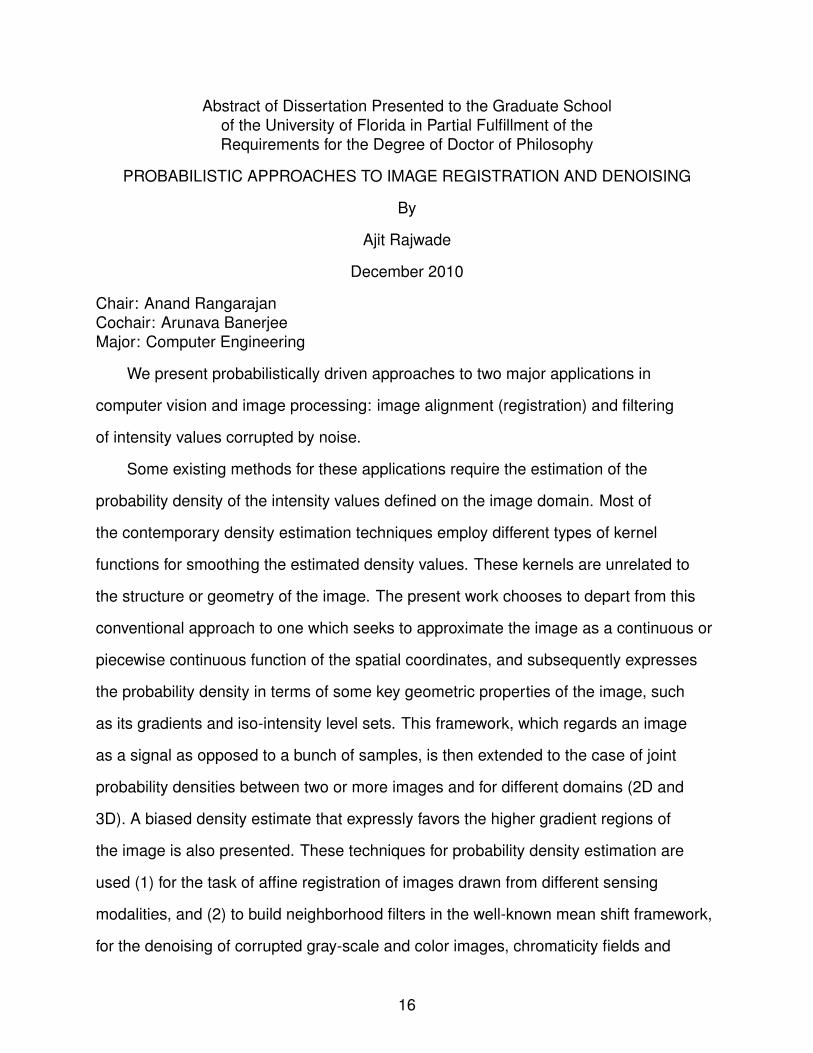
PROBABILISTIC APPROACHES TO IMAGE REGISTRATION AND DENOISING
By
Ajit Rajwade
December 2010
Chair: Anand RangarajanCochair: Arunava BanerjeeMajor: Computer Engineering
We present probabilistically driven approaches to two major applications in
computer vision and image processing: image alignment (registration) and filtering
of intensity values corrupted by noise.
Some existing methods for these applications require the estimation of the
probability density of the intensity values defined on the image domain. Most of
the contemporary density estimation techniques employ different types of kernel
functions for smoothing the estimated density values. These kernels are unrelated to
the structure or geometry of the image. The present work chooses to depart from this
conventional approach to one which seeks to approximate the image as a continuous or
piecewise continuous function of the spatial coordinates, and subsequently expresses
the probability density in terms of some key geometric properties of the image, such
as its gradients and iso-intensity level sets. This framework, which regards an image
as a signal as opposed to a bunch of samples, is then extended to the case of joint
probability densities between two or more images and for different domains (2D and
3D). A biased density estimate that expressly favors the higher gradient regions of
the image is also presented. These techniques for probability density estimation are
used (1) for the task of affine registration of images drawn from different sensing
modalities, and (2) to build neighborhood filters in the well-known mean shift framework,
for the denoising of corrupted gray-scale and color images, chromaticity fields and
16
gray-scale video. Using our new density estimators, we demonstrate improvement in the
performance of these applications. A new approach for the estimation of the probability
density of spherical data is also presented, taking into account the fact that the source of
such data are commonly known or assumed to be Euclidean, particularly within the field
of image analysis.
We also develop two patch-based image denoising algorithms that revisit the old
patch-based singular value decomposition (SVD) technique proposed in the seventies.
Noise does not affect only the singular values of an image patch, but also severely
affects its SVD bases leading to poor quality denoising if those bases are used. With
this in mind, we provide motivation for manipulating the SVD bases of the image patches
for improving denoising performance. To this end, we develop a probabilistic non-local
framework which learns spatially adaptive orthonormal bases that are derived by
exploiting the similarity between patches from different regions of an image. These
bases act as a common SVD for the group of patches similar to any reference patch
in the image. The reference image patches are then filtered by projection onto these
learned bases, manipulation of the transform coefficients and inversion of the transform.
We present or use principled criteria for the notion of similarity between patches under
noise and manipulation of the coefficients, assuming a fixed known noise model. The
several experimental results reported show that our method is simple and efficient,
it yields excellent performance as measured by standard image quality metrics, and
has principled parameter settings driven by statistical properties of the natural images
and the assumed noise models. We term this technique the non-local SVD (NL-SVD)
and extend it to produce a second, improved algorithm based upon the higher order
singular value decomposition (HOSVD). The HOSVD-based technique filters similar
patches jointly and produces denoising results that are better than most existing popular
methods and very close to the state of the art technique in the field of image denoising.
17
CHAPTER 1INTRODUCTION
Image analysis is a flourishing field that has made great progress in the past few
decades. Techniques from image analysis have been employed in fields as diverse as
medicine, mechanical engineering, remote sensing, biometric identification, pathology
and cell biology, molecular chemistry and lithography. An incomplete list of the key
problems that current researchers in the field are working on, includes (1) image
inpainting, (2) image denoising and restoration under various degradation models such
as defocus blur or motion blur, fog or haze, rain etc., (3) alignment of images of an object
sensed from different viewpoints potentially from different sensing modalities (called as
rigid or affine image registration), and possibly with nontrivial deformations of the object
itself, especially in applications involving medical imaging or face recognition (called as
non-rigid registration), (4) tomography, (5) image fusion or mosaicing, (6) segmentation
of images into coherent parts or segments, and (7) object recognition under different
views or lighting conditions.
Many of these techniques heavily employ statistical or probabilistic approaches.
A fundamental component of all such approaches is the estimation of the probability
density function (hereafter referred to as the PDF) of the intensity values of the image
defined at different points on the image domain. There exist several techniques for
PDF estimation in the literature. A common component of all of these techniques is
the estimation of frequency counts of the different values of the intensity followed by
smoothing or interpolation between these values, using kernel functions, yielding a
smoothed PDF estimate. These kernels are not related to the geometry of the image
in any manner. This thesis takes the opposite approach based on actually taking into
account the fact that the image is a geometric object (or a ‘signal’ as opposed to a
‘bunch of samples’) and interpolates the available samples to create a continuous image
representation, which is used in itself for PDF estimation. The use of the interpolant
18

produces a smoothed estimate that obviates the need for a kernel and critical kernel
parameters such as the bandwidth. Moreover this method of building a PDF evolves a
clear relationship between probabilistic quantities (such as the PDF itself) and geometric
entities (such as the gradients and the level sets). This estimator is discussed in Chapter
2, following a literature review of contemporary PDF estimators. In Chapters 3 and 4
respectively, the new PDF estimator is employed for two applications - image registration
under affine transformations, and denoising of various types of images affected primarily
by independent and identically distributed noise. The former application considers
images acquired possibly under different lighting conditions or different modalities such
as MR-T1, MR-T2, MR-PD (three different magnetic resonance imaging modalities). The
proposed PDF estimator produces results that are more robust than other techniques
under fine intensity quantization and under image noise. The denoising technique
in Chapter 4 (an interpolant driven local neighborhood method in the mean-shift
framework) is tested on gray-scale images, color images, chromaticity fields and
gray-scale video. For gray-scale and color images, the proposed PDF estimator
produces better denoising results even when the neighborhood for averaging and
the smoothing parameters are small. In Chapter 5, the thesis also discusses a related
problem in the field of spherical (or directional) statistics where the samples are points
on a unit sphere. These data are usually obtained as some function computed from the
original data which are usually known or assumed to lie in Euclidean space. Examples
include chromaticity vectors of color images which are unit-normalized versions of the
red-green-blue (RGB) values output by a camera. In this work, an estimator is presented
which does not impose a kernel directly on the unit vectors, but which uses existing
estimators in the original Euclidean space following random variable transformation.
Chapter 6 presents a detailed overview of contemporary image denoising
techniques. In chapter 7, we propose a probabilistic technique that starts off by revisiting
the image singular value decomposition (SVD). We perform experiments with global
19
and local image SVD and propose different ways to manipulate the SVD bases of
noisy image patches, or the coefficients of image patches when projected onto these
bases. We discuss the inefficacy of some of these manipulations, but demonstrate
that replacement of the image patch SVD by a common basis that represents an
ensemble of patches which are all similar to a reference patch, yields excellent filtering
performance. In this technique, which we call the non-local SVD (NL-SVD), a different
basis is produced at every pixel. We present a notion of patch similarity under noise,
which makes use of the properties of the noise model. The actual filtering is performed
at the patch level by projecting the patches onto the basis tuned for that patch, followed
by subsequent modification of the projection coefficients, and inversion of the transform.
Our technique is thus simple, elegant and efficient and it yields performance competitive
with the current state of the art. We also present a second and improved algorithm that
employs the higher-order singular value decomposition (HOSVD), an extension of the
SVD to higher order matrices.
While the research on image filtering has been extensive, there is very little
literature on automated estimation of the parameters of the filtering algorithms (i.e.
without reference to the true, clean image which is unknown in practical denoising
scenarios). In Chapter 8, we present a new statistically driven criterion for automated
filter parameter selection under the assumption that the noise is i.i.d. with a loose
lower bound on its variance. The criterion measures the statistical similarity between
non-overlapping patches of the residual image (the difference between the noisy and
the denoised image). The criterion is empirically seen to correlate well with known
full-reference quality measures (i.e. those that measure the error between the denoised
image and the true image). We test the criterion in conjunction with the NLMeans
algorithm [2] and the total variation PDE for selecting the smoothing parameter in these
methods.
20
CHAPTER 2PROBABILITY DENSITY WITH ISOCONTOURS AND ISOSURFACES
2.1 Overview of Existing PDF Estimators
The most commonly used PDF estimators include the histogram, the frequency
polygon, the Parzen window (or kernel) density estimator, the Gaussian mixture model,
and the much more recent wavelet-based density estimator. In the following, we briefly
review key properties of each. The review material, presented here for the sake of
completeness, is a brief summary of what is found in standard textbooks on the topic
such as [3] and [4].
2.1.1 The Histogram Estimator
The histogram-based density estimator p(x) for a density p(x) is defined as follows:
p(x) =F (bj+1)− F (bj)
nh(2–1)
where (bj , bj+1] defines a bin-boundary, h denotes the bin-width, F (bk) denotes the
number of samples whose value is less than or equal to bk and n is the total number of
samples. The histogram estimator is the simplest and the most popular one owing to
its simplicity. However it has a number of problems. Firstly, the estimates its produces
are always non-differentiable, even though the underlying density may be differentiable.
The estimate is highly sensitive to the choice of bin boundaries and more importantly
to the choice of the bin-width h. Using a high value of h produces a highly biased (or
over-smoothed) estimate, whereas a very small value of h leads to the problem of very
high variability of the estimate for small changes in the sample values. This tradeoff is
another instance of the classic bias-variance dilemma in machine learning. The specific
expressions for the bias and variance of this estimator are given as follows (due to [4]):
Bias(p(x)) =h − 2x + 2bj
2p′(x) +O(h2)forx ∈ (bj , bj+1] (2–2)
Variance(p(x)) =f (x)
nh+O(
1
n). (2–3)
21
The expressions clearly indicate the quadratic increase in bias with increase in h, and
the increase in variance inversely proportional to h. Also clear is the fact that the bias
problem is more pronounced for densities with higher derivative values.
The quality of a density estimator is often given by its mean squared error (MSE)
which is given as follows for the histogram (due to [4]):
MSE[p(x)] = Variance(p(x)) + Bias2(p(x)) (2–4)
=f (x)
nh+ Kp′(x)2 +O(
1
n) +O(h3). (2–5)
Upon integrating the MSE across x , we get the mean integrated square error (MSE),
which is given as (due to [4]):
MISE[p(x)] =1
nh+O(
1
n) +O(h3) +
h2∫p′(x)2dx
12(2–6)
The bin-width which minimizes the MISE is shown to be O(n−1/3) and inversely
proportional to∫p′(x)2dx , leading to an asymptotic MISE value which is O(n−2/3)
[4]. This indicates that the optimal rate of convergence of a histogram-based density
estimator is O(n−2/3).
2.1.2 The Frequency Polygon
Histograms are by definition piecewise constant density estimators. A frequency
polygon is simply a piecewise linear extension to the simple histogram and is obtained
by straightforward linear interpolation in between the estimated density values defined at
the midpoints of adjacent bins. This innocuous change produces an MISE value with a
smaller bias term (O(h2) as opposed to the earlier O(h)). The analysis in [4] which uses
the bin-width value that optimizes the MISE, indicates an improved convergence rate of
O(n−4/5) as opposed to the earlier O(n−2/3).
2.1.3 Kernel Density Estimators
To alleviate the non-differentiability of the histogram and the frequency polygon,
kernel density estimators build a differentiable kernel centered at every sample point.
22
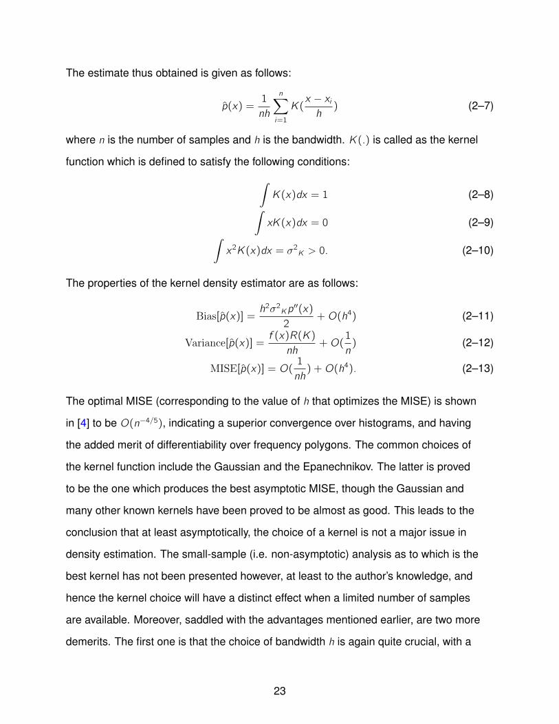
The estimate thus obtained is given as follows:
p(x) =1
nh
n∑i=1
K(x − xih) (2–7)
where n is the number of samples and h is the bandwidth. K(.) is called as the kernel
function which is defined to satisfy the following conditions:∫K(x)dx = 1 (2–8)∫xK(x)dx = 0 (2–9)∫
x2K(x)dx = σ2K > 0. (2–10)
The properties of the kernel density estimator are as follows:
Bias[p(x)] =h2σ2Kp
′′(x)
2+O(h4) (2–11)
Variance[p(x)] =f (x)R(K)
nh+O(
1
n) (2–12)
MISE[p(x)] = O(1
nh) +O(h4). (2–13)
The optimal MISE (corresponding to the value of h that optimizes the MISE) is shown
in [4] to be O(n−4/5), indicating a superior convergence over histograms, and having
the added merit of differentiability over frequency polygons. The common choices of
the kernel function include the Gaussian and the Epanechnikov. The latter is proved
to be the one which produces the best asymptotic MISE, though the Gaussian and
many other known kernels have been proved to be almost as good. This leads to the
conclusion that at least asymptotically, the choice of a kernel is not a major issue in
density estimation. The small-sample (i.e. non-asymptotic) analysis as to which is the
best kernel has not been presented however, at least to the author’s knowledge, and
hence the kernel choice will have a distinct effect when a limited number of samples
are available. Moreover, saddled with the advantages mentioned earlier, are two more
demerits. The first one is that the choice of bandwidth h is again quite crucial, with a
23
large h producing a high bias and a small h producing a high variance. Also, as per [3]
(Section 3.3.2), the ideal width value for minimizing the mean integrated squared error
between the true and estimated density is itself dependent upon the second derivative
of the (unknown) true density. This result therefore does not give any indication to a
practitioner about what the true bandwidth should be. Hence, the typical method to
estimate a bandwidth is a K -fold cross-validation based approach which turns out to be
both computationally expensive and quite error-prone. Secondly, in many applications,
the domain is bounded. However, the estimates produced by this method yield false
values on the boundary of such domains leading to large localized errors (especially if
kernels with unbounded support are used).
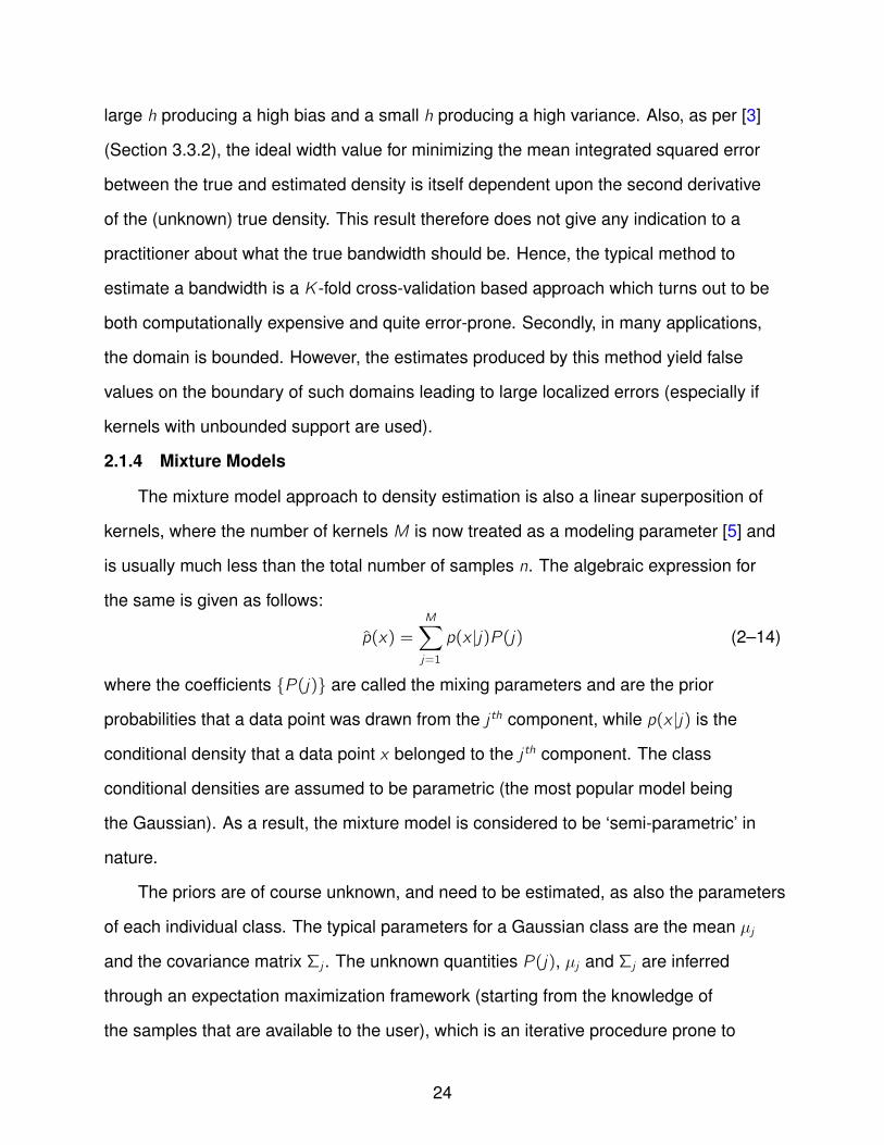
2.1.4 Mixture Models
The mixture model approach to density estimation is also a linear superposition of
kernels, where the number of kernels M is now treated as a modeling parameter [5] and
is usually much less than the total number of samples n. The algebraic expression for
the same is given as follows:
p(x) =
M∑j=1
p(x |j)P(j) (2–14)
where the coefficients P(j) are called the mixing parameters and are the prior
probabilities that a data point was drawn from the j th component, while p(x |j) is the
conditional density that a data point x belonged to the j th component. The class
conditional densities are assumed to be parametric (the most popular model being
the Gaussian). As a result, the mixture model is considered to be ‘semi-parametric’ in
nature.
The priors are of course unknown, and need to be estimated, as also the parameters
of each individual class. The typical parameters for a Gaussian class are the mean µj
and the covariance matrix Σj . The unknown quantities P(j), µj and Σj are inferred
through an expectation maximization framework (starting from the knowledge of
the samples that are available to the user), which is an iterative procedure prone to
24

local minima. The choice of the number of components, i.e. M, is also known to be
quite critical, with a very small value leading to inexpressive density estimates. Large
values for M reduce the efficiency of the mixture model over the simple kernel density
estimator.
2.1.5 Wavelet-Based Density Estimators
These estimators have been introduced relatively recently and are inspired
by the overwhelming success of wavelets in function approximation. An excellent
tutorial introduction to wavelet density estimation exists in [6] and [7], from which the
following material is summarized. Traditionally, a density estimate p(x) (for a true
underlying density p(x)) in this paradigm is expressed in the following manner, as a
linear combination of mother and father wavelet bases (φ(.) and ψ(.) respectively):
p(x) =∑L,k
αL,kφL,k(x) +∞∑j≥L,k
βj ,kψj ,k(x) (2–15)
where αL,k and βj ,k are the coefficients of expansion respectively. Note that the level L
indicates the coarsest scale. The basis functions at a resolution j are expressed in the
following manner:
φjk(x) = 2j/2φ(2jx − k) (2–16)
ψjk(x) = 2j/2ψ(2jx − k). (2–17)
The indices j (or j0) and k are the translation and scale indices respectively. The
coefficients of the entire wavelet expansion are given by the following formulae:
αL,k =
∫ +∞−∞
φL,k(x)p(x)dx (2–18)
βj ,k =
∫ +∞−∞
ψj ,k(x)p(x)dx (2–19)
and in practice are estimated as follows:
αL,k =1
n
n∑i=1
φL,k(xi) (2–20)
25
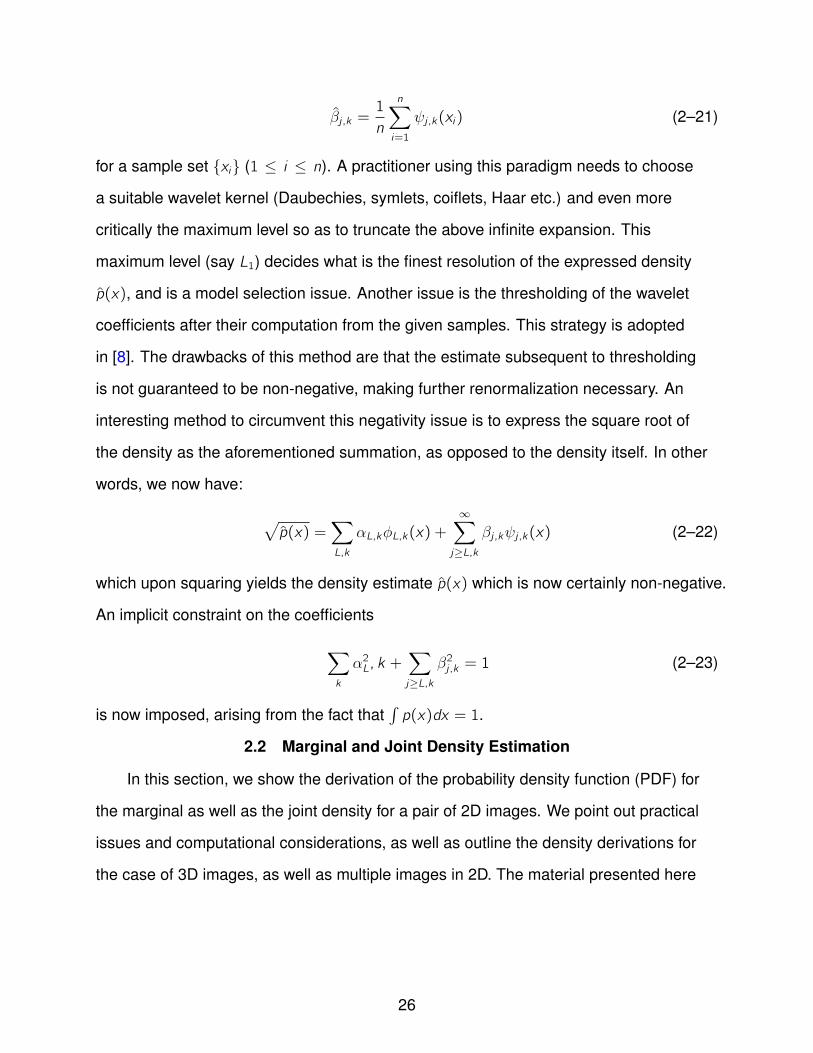
βj ,k =1
n
n∑i=1
ψj ,k(xi) (2–21)
for a sample set xi (1 ≤ i ≤ n). A practitioner using this paradigm needs to choose
a suitable wavelet kernel (Daubechies, symlets, coiflets, Haar etc.) and even more
critically the maximum level so as to truncate the above infinite expansion. This
maximum level (say L1) decides what is the finest resolution of the expressed density
p(x), and is a model selection issue. Another issue is the thresholding of the wavelet
coefficients after their computation from the given samples. This strategy is adopted
in [8]. The drawbacks of this method are that the estimate subsequent to thresholding
is not guaranteed to be non-negative, making further renormalization necessary. An
interesting method to circumvent this negativity issue is to express the square root of
the density as the aforementioned summation, as opposed to the density itself. In other
words, we now have:
√p(x) =
∑L,k
αL,kφL,k(x) +∞∑j≥L,k
βj ,kψj ,k(x) (2–22)
which upon squaring yields the density estimate p(x) which is now certainly non-negative.
An implicit constraint on the coefficients
∑k
α2L, k +∑j≥L,k
β2j ,k = 1 (2–23)
is now imposed, arising from the fact that∫p(x)dx = 1.
2.2 Marginal and Joint Density Estimation
In this section, we show the derivation of the probability density function (PDF) for
the marginal as well as the joint density for a pair of 2D images. We point out practical
issues and computational considerations, as well as outline the density derivations for
the case of 3D images, as well as multiple images in 2D. The material presented here
26
is taken from the author’s previous publications [9], [10] and [11]1 . The major difference
between the approach presented here and that of all the four techniques described
in previous subsections lies in this: the proposed approach really regards an image
(signal) as an image (a signal) and not a bunch of samples that can be re-arranged
without affecting the density estimate. Therefore essential properties on the signal
(image) can be directly incorporated into the estimation procedure itself.
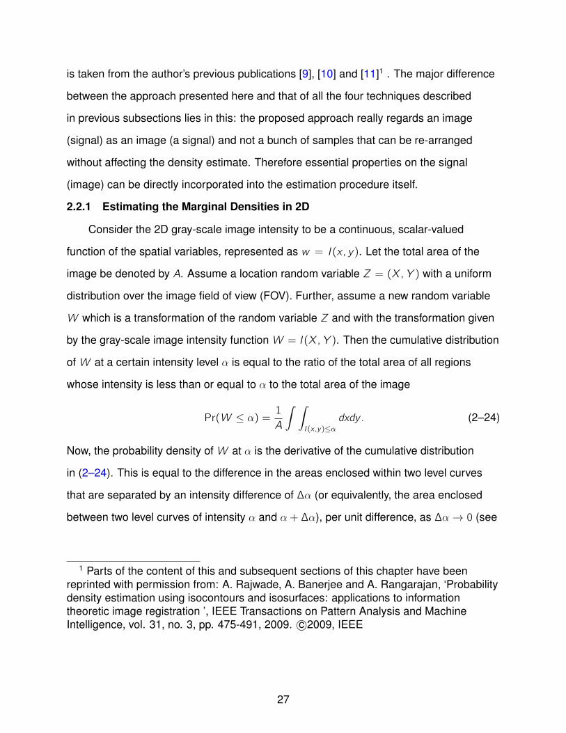
2.2.1 Estimating the Marginal Densities in 2D
Consider the 2D gray-scale image intensity to be a continuous, scalar-valued
function of the spatial variables, represented as w = I (x , y). Let the total area of the
image be denoted by A. Assume a location random variable Z = (X ,Y ) with a uniform
distribution over the image field of view (FOV). Further, assume a new random variable
W which is a transformation of the random variable Z and with the transformation given
by the gray-scale image intensity functionW = I (X ,Y ). Then the cumulative distribution
ofW at a certain intensity level α is equal to the ratio of the total area of all regions
whose intensity is less than or equal to α to the total area of the image
Pr(W ≤ α) =1
A
∫ ∫I (x ,y)≤α
dxdy . (2–24)
Now, the probability density ofW at α is the derivative of the cumulative distribution
in (2–24). This is equal to the difference in the areas enclosed within two level curves
that are separated by an intensity difference of ∆α (or equivalently, the area enclosed
between two level curves of intensity α and α + ∆α), per unit difference, as ∆α → 0 (see
1 Parts of the content of this and subsequent sections of this chapter have beenreprinted with permission from: A. Rajwade, A. Banerjee and A. Rangarajan, ‘Probabilitydensity estimation using isocontours and isosurfaces: applications to informationtheoretic image registration ’, IEEE Transactions on Pattern Analysis and MachineIntelligence, vol. 31, no. 3, pp. 475-491, 2009. c©2009, IEEE
27
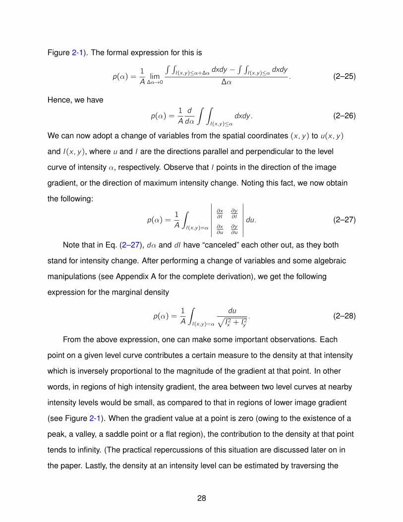
Figure 2-1). The formal expression for this is
p(α) =1
Alim∆α→0
∫ ∫I (x ,y)≤α+∆α
dxdy −∫ ∫I (x ,y)≤α
dxdy
∆α. (2–25)
Hence, we have
p(α) =1
A
d
dα
∫ ∫I (x ,y)≤α
dxdy . (2–26)
We can now adopt a change of variables from the spatial coordinates (x , y) to u(x , y)
and I (x , y), where u and I are the directions parallel and perpendicular to the level
curve of intensity α, respectively. Observe that I points in the direction of the image
gradient, or the direction of maximum intensity change. Noting this fact, we now obtain
the following:
p(α) =1
A
∫I (x ,y)=α
∣∣∣∣∣∣∣∂x∂I
∂y∂I
∂x∂u
∂y∂u
∣∣∣∣∣∣∣ du. (2–27)
Note that in Eq. (2–27), dα and dI have “canceled” each other out, as they both
stand for intensity change. After performing a change of variables and some algebraic
manipulations (see Appendix A for the complete derivation), we get the following
expression for the marginal density
p(α) =1
A
∫I (x ,y)=α
du√I 2x + I
2y
. (2–28)
From the above expression, one can make some important observations. Each
point on a given level curve contributes a certain measure to the density at that intensity
which is inversely proportional to the magnitude of the gradient at that point. In other
words, in regions of high intensity gradient, the area between two level curves at nearby
intensity levels would be small, as compared to that in regions of lower image gradient
(see Figure 2-1). When the gradient value at a point is zero (owing to the existence of a
peak, a valley, a saddle point or a flat region), the contribution to the density at that point
tends to infinity. (The practical repercussions of this situation are discussed later on in
the paper. Lastly, the density at an intensity level can be estimated by traversing the
28
level curve(s) at that intensity and integrating the reciprocal of the gradient magnitude.
One can obtain an estimate of the density at several intensity levels (at intensity spacing
of h from each other) across the entire intensity range of the image.
2.2.2 Related Work
A similar density estimator has also been developed by another group of researchers
[12], completely independently of this work. Their density estimator is motivated
exclusively by random variable transformations and does not incorporate the notion
of level sets. Furthermore, apart from differences in the derivation of the results, there
are differences in implementation. Moreover the applications they have targeted are
mainly image segmentation, particularly in the biomedical domain [13]. Similar notions
of densities obtained from random variable transformations have been mentioned in [14]
in the context of histogram preserving continuous transformations, with applications to
studying different projections of 3D models. However, in their actual implementation,
only digital samples are used, and there is no notion of any joint statistics. The density
estimator presented in this thesis was specifically developed in the context of an image
registration application (more about this in Chapter 3), and has been extended for
various special cases such as images defined in 3D, two or more than two images in
2D, and biased density estimators in 2D as well as 3D (as will been seen in subsequent
sections of this chapter).
2.2.3 Other Methods for Derivation
There exist at least two other methods of deriving the expression above, which are
discussed below.
1. Using Dirac-delta functions: The Dirac-delta function (with its domain being thereal line) is defined as follows:
δ(x) = +∞( if x = 0) (2–29)= 0( if x 6= 0)
29

in such a way that ∫ +∞−∞
δ(x)dx = 1. (2–30)
The delta function has analogous definitions in higher dimensions. It is awell-known property of the delta function (in any dimension) that∫ +∞
−∞f (~x)δ(I (~x))d~x =
∫I−1(0)
f (~x)du
|∇I (~x)|. (2–31)
Setting f (~x) to be unity throughout and considering that I (~x) is the image function,it is easy to see that
p(I (~x) = α) =
∫δ(I (~x)− α)dx =
∫I−1(0)
du
|∇I (~x)|. (2–32)
2. An intuitive geometric approach: Again consider the 2D gray-scale imageintensity to be a continuous, scalar-valued function of the spatial variables,represented as z = I (x , y). Assuming locations are iid, the cumulative distributionat a certain intensity level α can be written as follows:
Pr(z < α) =1
A
∫∫z<α
dxdy . (2–33)
Now, the probability density at α is the derivative of the cumulative distribution.This is equal to the difference in the areas enclosed within two level curves thatare separated by an intensity difference of ∆α (or equivalently, the area enclosedbetween two level curves of intensity α and α + ∆α), per unit difference, as∆α → 0 (see Figure (2-1)). At every location (x , y) along the level curve at α,the perpendicular distance (in terms of spatial coordinates) to the level curve atα + ∆α is given as ∆α
g(x ,y)where g(x , y) stands for the magnitude of the intensity
gradient at (x , y). Hence the total area enclosed between the two level curves canbe calculated as this distance integrated all along the contour at α. Denoting thetangent to the level curve as u, and taking the limit as ∆α → 0, we obtain the sameexpression.
2.2.4 Estimating the Joint Density
Consider two images represented as continuous scalar valued functions w1 =
I1(x , y) and w2 = I2(x , y), whose overlap area is A. As before, assume a location
random variable Z = X ,Y with a uniform distribution over the (overlap) field of view.
Further, assume two new random variablesW1 andW2 which are transformations of
the random variable Z and with the transformations given by the gray-scale image
intensity functionsW1 = I1(X ,Y ) andW2 = I2(X ,Y ). Let the set of all regions whose
30
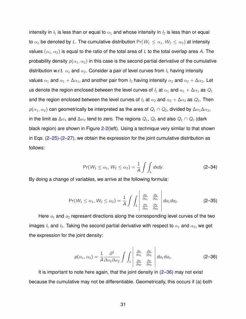
intensity in I1 is less than or equal to α1 and whose intensity in I2 is less than or equal
to α2 be denoted by L. The cumulative distribution Pr(W1 ≤ α1,W2 ≤ α2) at intensity
values (α1,α2) is equal to the ratio of the total area of L to the total overlap area A. The
probability density p(α1,α2) in this case is the second partial derivative of the cumulative
distribution w.r.t. α1 and α2. Consider a pair of level curves from I1 having intensity
values α1 and α1 + ∆α1, and another pair from I2 having intensity α2 and α2 + ∆α2. Let
us denote the region enclosed between the level curves of I1 at α1 and α1 + ∆α1 as Q1
and the region enclosed between the level curves of I2 at α2 and α2 + ∆α2 as Q2. Then
p(α1,α2) can geometrically be interpreted as the area of Q1 ∩ Q2, divided by ∆α1∆α2,
in the limit as ∆α1 and ∆α2 tend to zero. The regions Q1, Q2 and also Q1 ∩ Q2 (dark
black region) are shown in Figure 2-2(left). Using a technique very similar to that shown
in Eqs. (2–25)-(2–27), we obtain the expression for the joint cumulative distribution as
follows:
Pr(W1 ≤ α1,W2 ≤ α2) =1
A
∫ ∫L
dxdy . (2–34)
By doing a change of variables, we arrive at the following formula:
Pr(W1 ≤ α1,W2 ≤ α2) =1
A
∫ ∫L
∣∣∣∣∣∣∣∂x∂u1
∂y∂u1
∂x∂u2
∂y∂u2
∣∣∣∣∣∣∣ du1du2. (2–35)
Here u1 and u2 represent directions along the corresponding level curves of the two
images I1 and I2. Taking the second partial derivative with respect to α1 and α2, we get
the expression for the joint density:
p(α1,α2) =1
A
∂2
∂α1∂α2
∫ ∫L
∣∣∣∣∣∣∣∂x∂u1
∂y∂u1
∂x∂u2
∂y∂u2
∣∣∣∣∣∣∣ du1du2. (2–36)
It is important to note here again, that the joint density in (2–36) may not exist
because the cumulative may not be differentiable. Geometrically, this occurs if (a) both
31
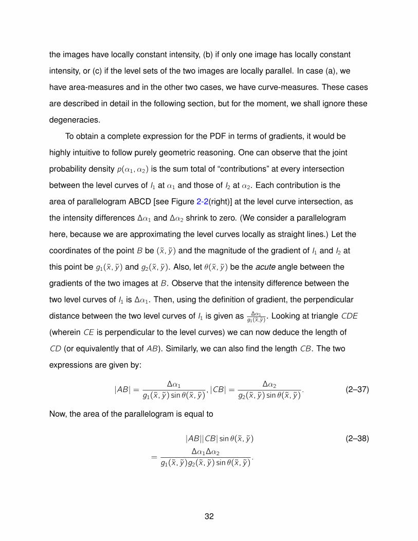
the images have locally constant intensity, (b) if only one image has locally constant
intensity, or (c) if the level sets of the two images are locally parallel. In case (a), we
have area-measures and in the other two cases, we have curve-measures. These cases
are described in detail in the following section, but for the moment, we shall ignore these
degeneracies.
To obtain a complete expression for the PDF in terms of gradients, it would be
highly intuitive to follow purely geometric reasoning. One can observe that the joint
probability density p(α1,α2) is the sum total of “contributions” at every intersection
between the level curves of I1 at α1 and those of I2 at α2. Each contribution is the
area of parallelogram ABCD [see Figure 2-2(right)] at the level curve intersection, as
the intensity differences ∆α1 and ∆α2 shrink to zero. (We consider a parallelogram
here, because we are approximating the level curves locally as straight lines.) Let the
coordinates of the point B be (x , y) and the magnitude of the gradient of I1 and I2 at
this point be g1(x , y) and g2(x , y). Also, let θ(x , y) be the acute angle between the
gradients of the two images at B. Observe that the intensity difference between the
two level curves of I1 is ∆α1. Then, using the definition of gradient, the perpendicular
distance between the two level curves of I1 is given as ∆α1g1(x ,y)
. Looking at triangle CDE
(wherein CE is perpendicular to the level curves) we can now deduce the length of
CD (or equivalently that of AB). Similarly, we can also find the length CB. The two
expressions are given by:
|AB| = ∆α1g1(x , y) sin θ(x , y)
, |CB| = ∆α2g2(x , y) sin θ(x , y)
. (2–37)
Now, the area of the parallelogram is equal to
|AB||CB| sin θ(x , y) (2–38)
=∆α1∆α2
g1(x , y)g2(x , y) sin θ(x , y).
32

With this, we finally obtain the following expression for the joint density:
p(α1,α2) =1
A
∑C
1
g1(x , y)g2(x , y) sin θ(x , y)(2–39)
where the set C represents the (countable) locus of all points where I1(x , y) = α1
and I2(x , y) = α2. It is easy to show through algebraic manipulations that Eqs. (2–36)
and (2–39) are equivalent formulations of the joint probability density p(α1,α2). These
results could also have been derived purely by manipulation of Jacobians (as done
while deriving marginal densities), and the derivation for the marginals could also have
proceeded following geometric intuitions.
The formula derived above tallies beautifully with intuition in the following ways.
Firstly, the area of the parallelogram ABCD (i.e. the joint density contribution) in regions
of high gradient [in either or both image(s)] is smaller as compared to that in the case of
regions with lower gradients. Secondly, the area of parallelogram ABCD (i.e. the joint
density contribution) is the least when the gradients of the two images are orthogonal
and maximum when they are parallel or coincident [see Figure 2-3(a)]. In fact, the
joint density tends to infinity in the case where either (or both) gradient(s) is (are)
zero, or when the two gradients align, so that sin θ is zero. The repercussions of this
phenomenon are discussed in the following section.
2.2.5 From Densities to Distributions
In the two preceding sub-sections, we observed the divergence of the marginal
density in regions of zero gradient, or of the joint density in regions where either (or
both) image gradient(s) is (are) zero, or when the gradients locally align. The gradient
goes to zero in regions of the image that are flat in terms of intensity, and also at peaks,
valleys and saddle points on the image surface. We can ignore the latter three cases
as they are a finite number of points within a continuum. The probability contribution
at a particular intensity in a flat region is proportional to the area of that flat region.
Some ad hoc approaches could involve simply “weeding out” the flat regions altogether,
33
but that would require the choice of sensitive thresholds. The key thing is to notice
that in these regions, the density does not exist but the probability distribution does.
So, we can switch entirely to probability distributions everywhere by introducing a
non-zero lower bound on the “values” of ∆α1 and ∆α2. Effectively, this means that
we always look at parallelograms representing the intersection between pairs of level
curves from the two images, separated by non-zero intensity difference, denoted
as, say, h. Since these parallelograms have finite areas, we have circumvented the
situation of choosing thresholds to prevent the values from becoming unbounded,
and the probability at α1,α2, denoted as p(α1,α2) is obtained from the areas of such
parallelograms. We term this area-based method of density estimation as AreaProb.
Later on in the paper, we shall show that the switch to distributions is principled and
does not reduce our technique to standard histogramming in any manner whatsoever.
The notion of an image as a continuous entity is one of the pillars of our approach.
We adopt a locally linear formulation in this paper, for the sake of simplicity, though
the technical contributions of this paper are in no way tied to any specific interpolant.
For each image grid point, we estimate the intensity values at its four neighbors within
a horizontal or vertical distance of 0.5 pixels. We then divide each square defined by
these neighbors into a pair of triangles. The intensities within each triangle can be
represented as a planar patch, which is given by the equation z1 = A1x + B1y + C1 in
I1. Iso-intensity lines at levels α1 and α1 + h within this triangle are represented by the
equations A1x +B1y +C1 = α1 and A1x +B1y +C1 = α1+ h (likewise for the iso-intensity
lines of I2 at intensities α2 and α2 + h, within a triangle of corresponding location). The
contribution from this triangle to the joint probability at (α1,α2), i.e. p(α1,α2) is the
area bounded by the two pairs of parallel lines, clipped against the body of the triangle
itself, as shown in Figure 2-7. In the case that the corresponding gradients from the two
images are parallel (or coincident), they enclose an infinite area between them, which
when clipped against the body of the triangle, yields a closed polygon of finite area, as
34

shown in Figure 2-7. When both the gradients are zero (which can be considered to be a
special case of gradients being parallel), the probability contribution is equal to the area
of the entire triangle. In the case where the gradient of only one of the images is zero,
the contribution is equal to the area enclosed between the parallel iso-intensity lines
of the other image, clipped against the body of the triangle (see Figure 2-7). Observe
that though we have to treat pathological regions specially (despite having switched to
distributions), we now do not need to select thresholds, nor do we need to deal with a
mixture of densities and distributions. The other major advantage is added robustness to
noise, as we are now working with probabilities instead of their derivatives, i.e. densities.
The issue that now arises is how the value of h may be chosen. It should be
noted that although there is no “optimal” h, our density estimate would convey more
and more information as the value of h is reduced (in complete contrast to standard
histogramming). In Figure 2-5, we have shown plots of our joint density estimate and
compared it to standard histograms for P equal to 16, 32, 64 and 128 bins in each
image (i.e. 322, 642 etc. bins in the joint), which illustrate our point clearly. We found
that the standard histograms had a far greater number of empty bins than our density
estimator, for the same number of intensity levels. The corresponding marginal discrete
distributions for the original retinogram image [1] for 16, 32, 64 and 128 bins are shown
in Figure 2-6.
2.2.6 Joint Density between Multiple Images in 2D
For the simultaneous registration of multiple (d > 2) images, the use of a single
d-dimensional joint probability has been advocated in previous literature [15], [16]. Our
joint probability derivation can be easily extended to the case of d > 2 images by using
similar geometric intuition to obtain the polygonal area between d intersecting pairs of
level curves [see Figure 2-3(right) for the case of d = 3 images]. Note here that the
d-dimensional joint distribution lies essentially in a 2D subspace, as we are dealing
with 2D images. A naıve implementation of such a scheme has a complexity of O(NPd)
35
where P is the number of intensity levels chosen for each image and N is the size of
each image. Interestingly, however, this exponential cost can be side-stepped by first
computing the at most (d(d−1)2)P2 points of intersection between pairs of level curves
from all d images with one another, for every pixel. Secondly, a graph can be created,
each of whose nodes is an intersection point. Nodes are linked by edges labeled with
the image number (say k th image) if they lie along the same iso-contour of that image. In
most cases, each node of the graph will have a degree of four (and in the unlikely case
where level curves from all images are concurrent, the maximal degree of a node will
be 2d). Now, this is clearly a planar graph, and hence, by Euler’s formula, we have the
number of (convex polygonal) faces F = d(d−1)2
∗ 4P2 − d(d−1)2P2 + 2 = O(P2d2), which
is quadratic in the number of images. The area of the polygonal faces are contributions
to the joint probability distribution. In a practical implementation, there is no requirement
to even create the planar graph. Instead, we can implement a simple incremental
face-splitting algorithm ([17], section 8.3). In such an implementation, we create a list of
faces F which is updated incrementally. To start with, F consists of just the triangular
face constituting the three vertices of a chosen half-pixel in the image. Next, we consider
a single level-line l at a time and split into two any face in F that l intersects. This
procedure is repeated for all level lines (separated by a discrete intensity spacing) of all
the d images. The final output is a listing of all polygonal faces F created by incremental
splitting which can be created in just O(FPd) time. The storage requirement can be
made polynomial by observing that for d images, the number of unique intensity tuples
will be at most FN in the worst case (as opposed to Pd ). Hence all intensity tuples can
be efficiently stored and indexed using a hash table.
2.2.7 Extensions to 3D
When estimating the probability density from 3D images, the choice of an optimal
smoothing parameter is a less critical issue, as a much larger number of samples
are available. However, at a theoretical level this still remains a problem, which would
36
worsen in the multiple image case. In 3D, the marginal probability can be interpreted as
the total volume sandwiched between two iso-surfaces at neighboring intensity levels.
The formula for the marginal density p(α) of a 3D image w = I (x , y , z) is given as
follows:
p(α) =1
V
d
dα
∫ ∫ ∫I (x ,y ,z)≤α
dxdydz . (2–40)
Here V is the volume of the image I (x , y , z). We can now adopt a change of variables
from the spatial coordinates x , y and z to u1(x , y , z), u2(x , y , z) and I (x , y , z), where I
is the perpendicular to the level surface (i.e. parallel to the gradient) and u1 and u2 are
mutually perpendicular directions parallel to the level surface. Noting this fact, we now
obtain the following:
p(α) =1
V
∫ ∫I (x ,y ,z)=α
∣∣∣∣∣∣∣∣∣∣∂x∂I
∂y∂I
∂z∂I
∂x∂u1
∂y∂u1
∂z∂u1
∂x∂u2
∂y∂u2
∂z∂u2
∣∣∣∣∣∣∣∣∣∣du1du2. (2–41)
Upon a series of algebraic manipulations just as before, we are left with the following
expression for p(α):
p(α) =1
V
∫ ∫I (x ,y ,z)=α
du1du2√( ∂I∂x)2 + ( ∂I
∂y)2 + ( ∂I
∂z)2. (2–42)
For the joint density case, consider two 3D images represented as w1 = I1(x , y , z)
and w2 = I2(x , y , z), whose overlap volume (the field of view) is V . The cumulative
distribution Pr(W1 ≤ α1,W2 ≤ α2) at intensity values (α1,α2) is equal to the ratio of
the total volume of all regions whose intensity in the first image is less than or equal
to α1 and whose intensity in the second image is less than or equal to α2, to the total
image volume. The probability density p(α1,α2) is again the second partial derivative
of the cumulative distribution. Consider two regions R1 and R2, where R1 is the region
trapped between level surfaces of the first image at intensities α1 and α1 + ∆α1, and R2
is defined analogously for the second image. The density is proportional to the volume
37
of the intersection of R1 and R2 divided by ∆α1 and ∆α2 when the latter two tend to zero.
It can be shown through some geometric manipulations that the area of the base of
the parallelepiped formed by the iso-surfaces is given as ∆α1∆α2| ~g1× ~g2| =∆α1∆α2
|g1g2 sin(θ)| , where ~g1
and ~g2 are the gradients of the two images, and θ is the angle between them. Let ~h be
a vector which points in the direction of the height of the parallelepiped (parallel to the
base normal, i.e. ~g1 × ~g2), and d~h be an infinitesimal step in that direction. Then the
probability density is given as follows:
p(α1,α2) =1
V
∂2
∂α1∂α2
∫ ∫ ∫Vs
dxdydz
=1
V
∂2
∂α1∂α2
∫ ∫ ∫Vs
d ~u1d ~u2d~h
|~g1 × ~g2|=1
V
∫C
d~h
|~g1 × ~g2|. (2–43)
In Eq. (2–43), ~u1 and ~u2 are directions parallel to the iso-surfaces of the two images, and
~h is their cross-product (and parallel to the line of intersection of the individual planes),
while C is the 3D space curve containing the points where I1 and I2 have values α1 and
α2 respectively and Vsdef= (x , y , z) : I1(x , y , z) ≤ α1, I2(x , y , z) ≤ α2.
2.2.8 Implementation Details for the 3D case
The density formulation for the 3D case suffers from the same problem of
divergence to infinity, as in the 2D case. Similar techniques can be employed, this
time using level surfaces that are separated by finite intensity gaps. To trace the level
surfaces, each cube-shaped voxel in the 3D image can be divided into 12 tetrahedra.
The apex of each tetrahedron is located at the center of the voxel and the base is
formed by dividing one of the six square faces of the cube by one of the diagonals of
that face [see Figure 2-8(a)]. Within each triangular face of each such tetrahedron, the
intensity can be assumed to be a linear function of location. Note that the intensities
in different faces of one and the same tetrahedron can thus be expressed by different
functions, all of them linear. Hence the iso-surfaces at different intensity levels within a
single tetrahedron are non-intersecting but not necessarily parallel. These level surfaces
at any intensity within a single tetrahedron turn out to be either triangles or quadrilaterals
38
in 3D. This interpolation scheme does have some bias in the choice of the diagonals
that divide the individual square faces. A scheme that uses 24 tetrahedra with the apex
at the center of the voxel, and four tetrahedra based on every single face, has no bias
of this kind [see Figure 2-8(b)]. However, we still used the former (and faster) scheme
as it is simpler and does not noticeably affect the results. Level surfaces are again
traced at a finite number of intensity values, separated by equal intensity intervals. The
marginal density contributions are obtained as the volumes of convex polyhedra trapped
in between consecutive level surfaces clipped against the body of individual tetrahedra.
The joint distribution contribution from each voxel is obtained by finding the volume of
the convex polyhedron resulting from the intersection of corresponding convex polyhedra
from the two images, clipped against the tetrahedra inside the voxel. We refer to this
scheme of finding joint densities as VolumeProb.
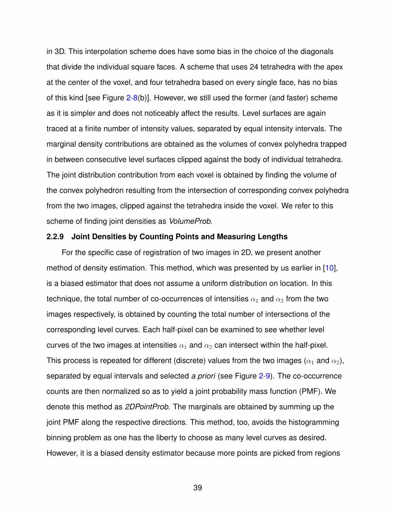
2.2.9 Joint Densities by Counting Points and Measuring Lengths
For the specific case of registration of two images in 2D, we present another
method of density estimation. This method, which was presented by us earlier in [10],
is a biased estimator that does not assume a uniform distribution on location. In this
technique, the total number of co-occurrences of intensities α1 and α2 from the two
images respectively, is obtained by counting the total number of intersections of the
corresponding level curves. Each half-pixel can be examined to see whether level
curves of the two images at intensities α1 and α2 can intersect within the half-pixel.
This process is repeated for different (discrete) values from the two images (α1 and α2),
separated by equal intervals and selected a priori (see Figure 2-9). The co-occurrence
counts are then normalized so as to yield a joint probability mass function (PMF). We
denote this method as 2DPointProb. The marginals are obtained by summing up the
joint PMF along the respective directions. This method, too, avoids the histogramming
binning problem as one has the liberty to choose as many level curves as desired.
However, it is a biased density estimator because more points are picked from regions
39

with high image gradient. This is because more level curves (at equi-spaced intensity
levels) are packed together in such areas. It can also be regarded as a weighted version
of the joint density estimator presented in the previous sub-section, with each point
weighted by the gradient magnitudes of the two images at that point as well as the sine
of the angle between them. Thus the joint PMF by this method is given as
p(α1,α2) =∂2
∂α1∂α2
1
K
∫ ∫D
g1(x , y)g2(x , y) sin θ(x , y)dxdy (2–44)
where D denotes the regions where I1(x , y) ≤ α1, I2(x , y) ≤ α2 and K is a normalization
constant. This simplifies to the following:
p(α1,α2) =1
K
∑C
1. (2–45)
Hence, we have p(α1,α2) =|C |K
, where C is the (countable) set of points where
I1(x , y) = α1 and I2(x , y) = α2. The marginal (biased) density estimates can be regarded
as lengths of the individual iso-contours. With this notion in mind, the marginal density
estimates are seen to have a close relation with the total variation of an image, which
is given by TV =∫I=α
|∇I (x , y)|dxdy [18]. We clearly have TV =∫I=αdu, by doing
the same change of variables (from x , y to u, I ) as in Eqs. (2–27) and (2–28), thus
giving us the length of the iso-contours at any given intensity level. In 3D, we consider
the segments of intersection of two iso-surfaces and calculate their lengths, which
become the PMF contributions. We refer to this as LengthProb [see Figure 2-10(a)].
Both 2DPointProb and LengthProb, however, require us to ignore those regions in which
level sets do not exist because the intensity function is flat, or those regions where level
sets from the two images are parallel. The case of flat regions in one or both images can
be fixed to some extent by slight blurring of the image. The case of aligned gradients
is trickier, especially if the two images are in complete registration. However, in the
multi-modality case or if the images are noisy/blurred, perfect registration is a rare
occurrence, and hence perfect alignment of level surfaces will rarely occur.
40
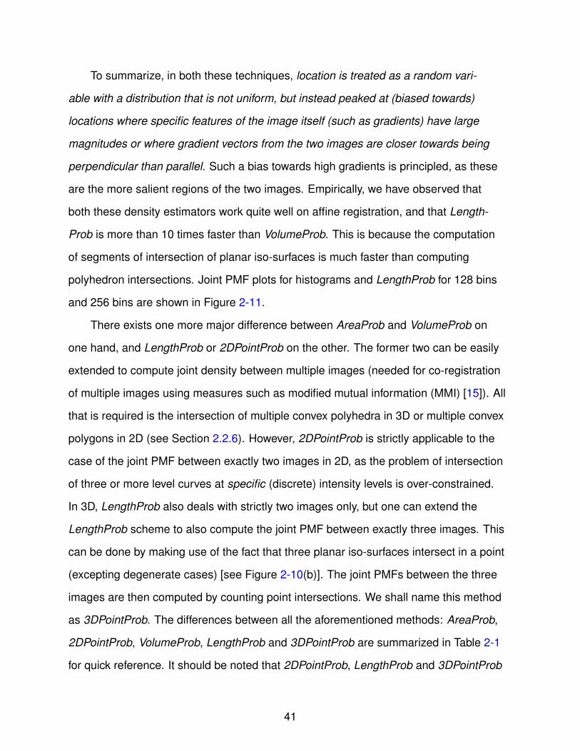
To summarize, in both these techniques, location is treated as a random vari-
able with a distribution that is not uniform, but instead peaked at (biased towards)
locations where specific features of the image itself (such as gradients) have large
magnitudes or where gradient vectors from the two images are closer towards being
perpendicular than parallel. Such a bias towards high gradients is principled, as these
are the more salient regions of the two images. Empirically, we have observed that
both these density estimators work quite well on affine registration, and that Length-
Prob is more than 10 times faster than VolumeProb. This is because the computation
of segments of intersection of planar iso-surfaces is much faster than computing
polyhedron intersections. Joint PMF plots for histograms and LengthProb for 128 bins
and 256 bins are shown in Figure 2-11.
There exists one more major difference between AreaProb and VolumeProb on
one hand, and LengthProb or 2DPointProb on the other. The former two can be easily
extended to compute joint density between multiple images (needed for co-registration
of multiple images using measures such as modified mutual information (MMI) [15]). All
that is required is the intersection of multiple convex polyhedra in 3D or multiple convex
polygons in 2D (see Section 2.2.6). However, 2DPointProb is strictly applicable to the
case of the joint PMF between exactly two images in 2D, as the problem of intersection
of three or more level curves at specific (discrete) intensity levels is over-constrained.
In 3D, LengthProb also deals with strictly two images only, but one can extend the
LengthProb scheme to also compute the joint PMF between exactly three images. This
can be done by making use of the fact that three planar iso-surfaces intersect in a point
(excepting degenerate cases) [see Figure 2-10(b)]. The joint PMFs between the three
images are then computed by counting point intersections. We shall name this method
as 3DPointProb. The differences between all the aforementioned methods: AreaProb,
2DPointProb, VolumeProb, LengthProb and 3DPointProb are summarized in Table 2-1
for quick reference. It should be noted that 2DPointProb, LengthProb and 3DPointProb
41
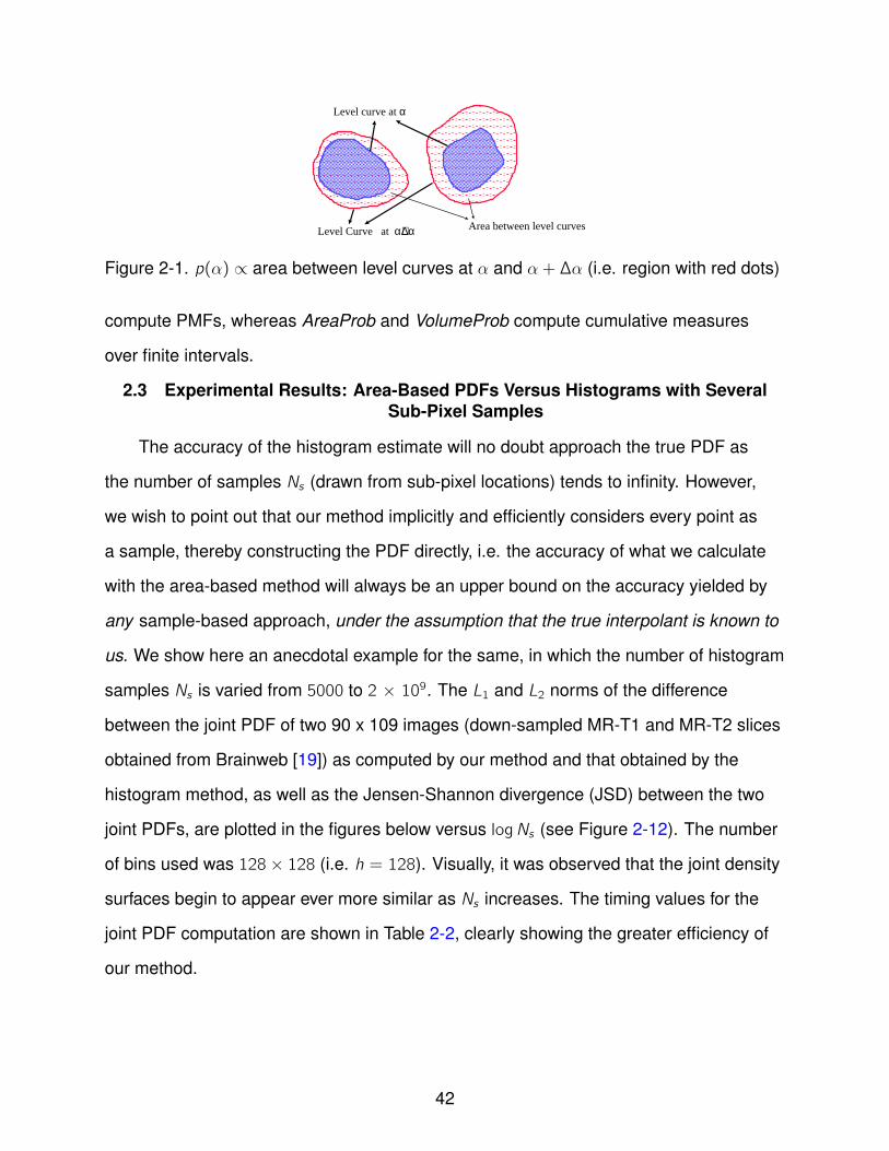
Level Curve at α+∆α
Level curve at α
Area between level curves
Figure 2-1. p(α) ∝ area between level curves at α and α+∆α (i.e. region with red dots)
compute PMFs, whereas AreaProb and VolumeProb compute cumulative measures
over finite intervals.
2.3 Experimental Results: Area-Based PDFs Versus Histograms with SeveralSub-Pixel Samples
The accuracy of the histogram estimate will no doubt approach the true PDF as
the number of samples Ns (drawn from sub-pixel locations) tends to infinity. However,
we wish to point out that our method implicitly and efficiently considers every point as
a sample, thereby constructing the PDF directly, i.e. the accuracy of what we calculate
with the area-based method will always be an upper bound on the accuracy yielded by
any sample-based approach, under the assumption that the true interpolant is known to
us. We show here an anecdotal example for the same, in which the number of histogram
samples Ns is varied from 5000 to 2 × 10⁹. The L1 and L2 norms of the difference
between the joint PDF of two 90 x 109 images (down-sampled MR-T1 and MR-T2 slices
obtained from Brainweb [19]) as computed by our method and that obtained by the
histogram method, as well as the Jensen-Shannon divergence (JSD) between the two
joint PDFs, are plotted in the figures below versus logNs (see Figure 2-12). The number
of bins used was 128× 128 (i.e. h = 128). Visually, it was observed that the joint density
surfaces begin to appear ever more similar as Ns increases. The timing values for the
joint PDF computation are shown in Table 2-2, clearly showing the greater efficiency of
our method.
42
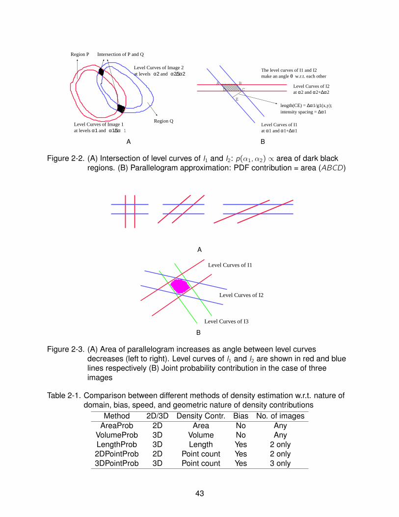
Level Curves of Image 1at levels α1 and α1+∆α1
Level Curves of Image 2at levels α2 and α2+∆α2
Region P
Region Q
Intersection of P and Q
A
A
D C
B
Level Curves of I1at α1 and α1+∆α1
The level curves of I1 and I2make an angle θ w.r.t. each other
E
Level Curves of I2at α2 and α2+∆α2
length(CE) = ∆α1/g1(x,y);intensity spacing = ∆α1
B
Figure 2-2. (A) Intersection of level curves of I1 and I2: p(α1,α2) ∝ area of dark blackregions. (B) Parallelogram approximation: PDF contribution = area (ABCD)
A
Level Curves of I1
Level Curves of I2
Level Curves of I3
B
Figure 2-3. (A) Area of parallelogram increases as angle between level curvesdecreases (left to right). Level curves of I1 and I2 are shown in red and bluelines respectively (B) Joint probability contribution in the case of threeimages
Table 2-1. Comparison between different methods of density estimation w.r.t. nature ofdomain, bias, speed, and geometric nature of density contributions
Method 2D/3D Density Contr. Bias No. of imagesAreaProb 2D Area No Any
VolumeProb 3D Volume No AnyLengthProb 3D Length Yes 2 only2DPointProb 2D Point count Yes 2 only3DPointProb 3D Point count Yes 3 only
43
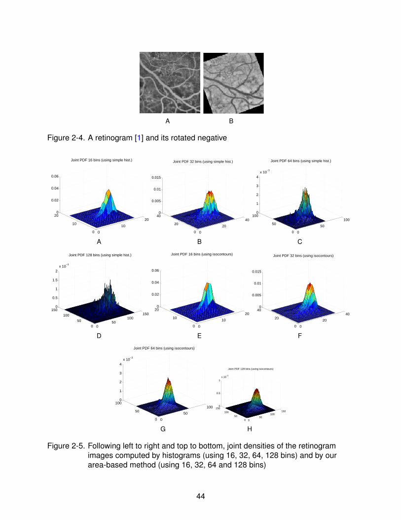
A B
Figure 2-4. A retinogram [1] and its rotated negative
0
10
20
0
10
200
0.02
0.04
0.06
Joint PDF 16 bins (using simple hist.)
A
0
20
40
0
20
400
0.005
0.01
0.015
Joint PDF 32 bins (using simple hist.)
B
0
50
100
0
50
1000
1
2
3
4x 10
−3
Joint PDF 64 bins (using simple hist.)
C
050
100150
0
50
100
1500
0.5
1
1.5
2x 10
−3
Joint PDF 128 bins (using simple hist.)
D
0
10
20
0
10
200
0.02
0.04
0.06
Joint PDF 16 bins (using isocontours)
E
0
20
40
0
20
400
0.005
0.01
0.015
Joint PDF 32 bins (using isocontours)
F
0
50
100
0
50
1000
1
2
3
4x 10
−3
Joint PDF 64 bins (using isocontours)
G
050
100150
0
50
100
1500
0.5
1x 10
−3
Joint PDF 128 bins (using isocontours)
H
Figure 2-5. Following left to right and top to bottom, joint densities of the retinogramimages computed by histograms (using 16, 32, 64, 128 bins) and by ourarea-based method (using 16, 32, 64 and 128 bins)
44
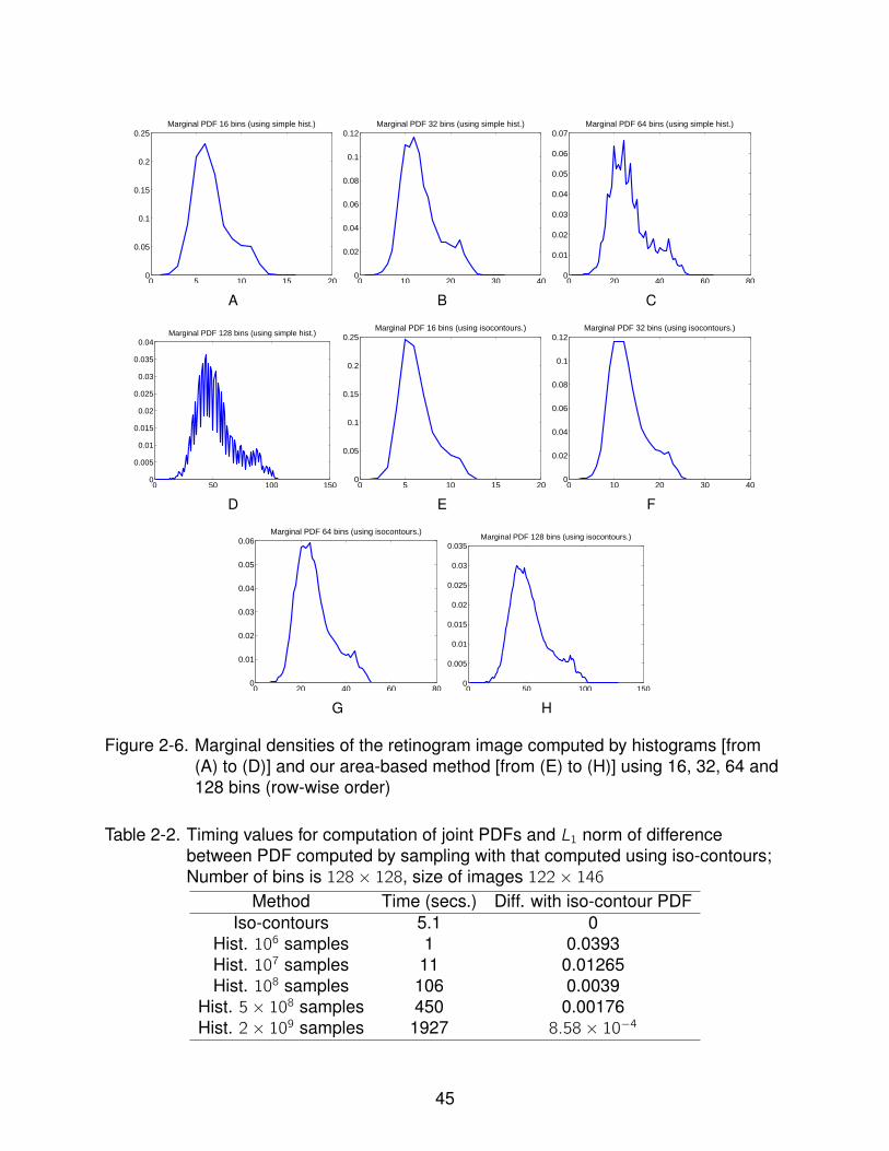
0 5 10 15 200
0.05
0.1
0.15
0.2
0.25Marginal PDF 16 bins (using simple hist.)
A0 10 20 30 40
0
0.02
0.04
0.06
0.08
0.1
0.12Marginal PDF 32 bins (using simple hist.)
B0 20 40 60 80
0
0.01
0.02
0.03
0.04
0.05
0.06
0.07Marginal PDF 64 bins (using simple hist.)
C
0 50 100 1500
0.005
0.01
0.015
0.02
0.025
0.03
0.035
0.04Marginal PDF 128 bins (using simple hist.)
D0 5 10 15 20
0
0.05
0.1
0.15
0.2
0.25Marginal PDF 16 bins (using isocontours.)
E0 10 20 30 40
0
0.02
0.04
0.06
0.08
0.1
0.12Marginal PDF 32 bins (using isocontours.)
F
0 20 40 60 800
0.01
0.02
0.03
0.04
0.05
0.06Marginal PDF 64 bins (using isocontours.)
G0 50 100 150
0
0.005
0.01
0.015
0.02
0.025
0.03
0.035Marginal PDF 128 bins (using isocontours.)
H
Figure 2-6. Marginal densities of the retinogram image computed by histograms [from(A) to (D)] and our area-based method [from (E) to (H)] using 16, 32, 64 and128 bins (row-wise order)
Table 2-2. Timing values for computation of joint PDFs and L1 norm of differencebetween PDF computed by sampling with that computed using iso-contours;Number of bins is 128× 128, size of images 122× 146
Method Time (secs.) Diff. with iso-contour PDFIso-contours 5.1 0
Hist. 106 samples 1 0.0393Hist. 107 samples 11 0.01265Hist. 108 samples 106 0.0039
Hist. 5× 10⁸ samples 450 0.00176Hist. 2× 10⁹ samples 1927 8.58× 10⁻⁴
45
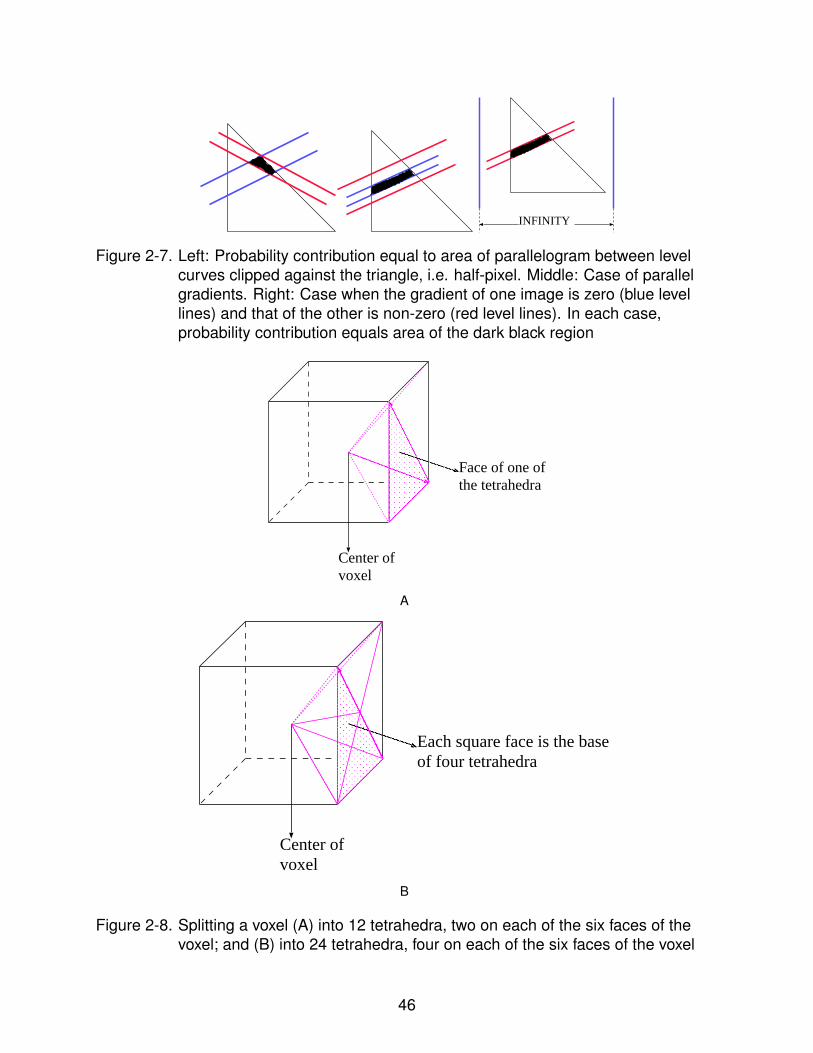
INFINITY
Figure 2-7. Left: Probability contribution equal to area of parallelogram between levelcurves clipped against the triangle, i.e. half-pixel. Middle: Case of parallelgradients. Right: Case when the gradient of one image is zero (blue levellines) and that of the other is non-zero (red level lines). In each case,probability contribution equals area of the dark black region
Center ofvoxel
Face of one ofthe tetrahedra
A
Center ofvoxel
Each square face is the baseof four tetrahedra
B
Figure 2-8. Splitting a voxel (A) into 12 tetrahedra, two on each of the six faces of thevoxel; and (B) into 24 tetrahedra, four on each of the six faces of the voxel
46

Neighbors ofgrid point
Pixel grid point
Square divided intotwo triangles
Iso-intensity line of I1 at α1
Iso-intensity line of I2 at α2
A vote for p(α1,α2)
A vote for p(α1+∆,α2+∆)
Figure 2-9. Counting level curve intersections within a given half-pixel
Line of intersectionof two planes
Planar Isosurfacesfrom the two images
A
Line of intersectionof two planes
Planar Isosurfacesfrom the three images
Point of intersection ofthree planes
B
Figure 2-10. Biased estimates in 3D: (A) Segment of intersection of planar iso-surfacesfrom the two images, (B) Point of intersection of planar iso-surfaces fromthe three images (each in a different color)
47
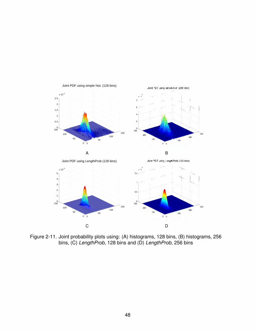
0
50
100
150
0
50
100
1500
0.5
1
1.5
2
2.5
x 10−3
Joint PDF using simple hist. (128 bins)
A B
0
50
100
150
0
50
100
1500
1
2
3
4
5
x 10−3
Joint PDF using LengthProb (128 bins)
C D
Figure 2-11. Joint probability plots using: (A) histograms, 128 bins, (B) histograms, 256bins, (C) LengthProb, 128 bins and (D) LengthProb, 256 bins
48
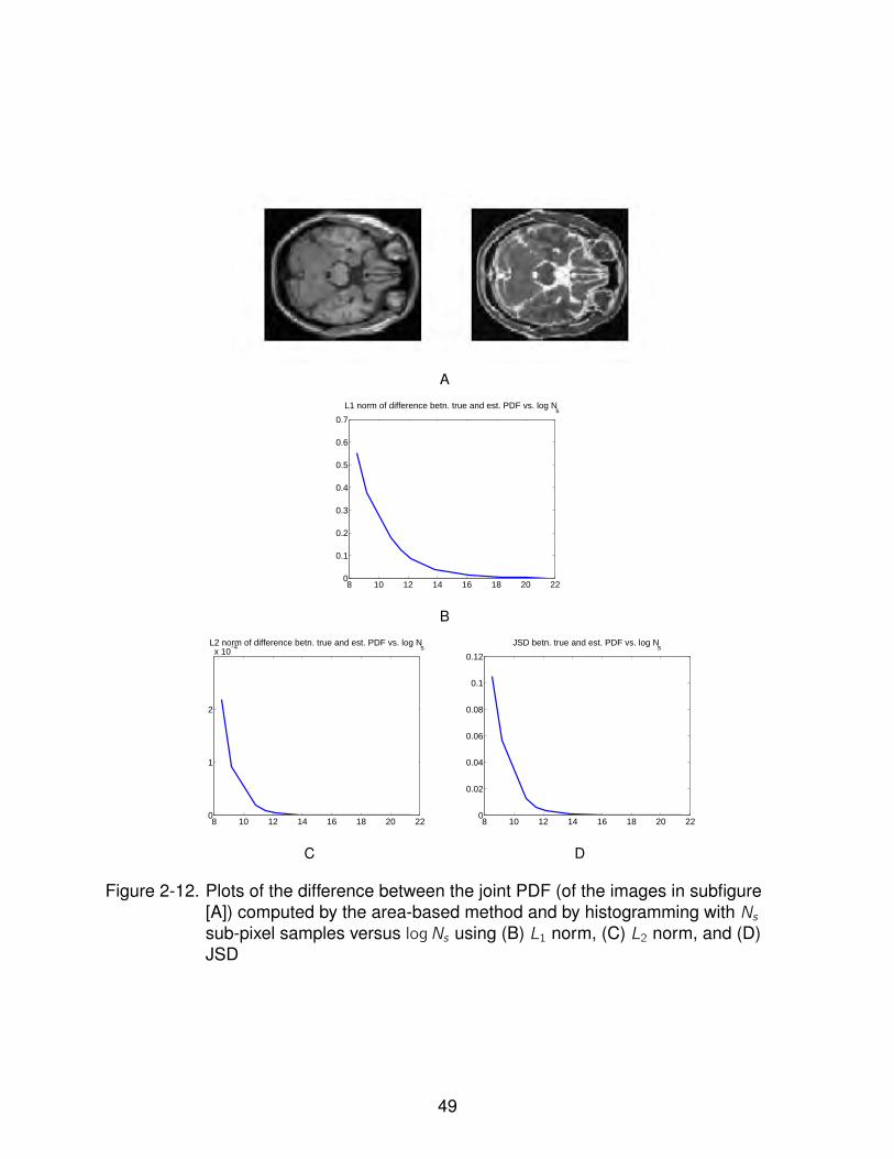
A
8 10 12 14 16 18 20 220
0.1
0.2
0.3
0.4
0.5
0.6
0.7
L1 norm of difference betn. true and est. PDF vs. log Ns
B
8 10 12 14 16 18 20 220
1
2
x 10−4
L2 norm of difference betn. true and est. PDF vs. log Ns
C
8 10 12 14 16 18 20 220
0.02
0.04
0.06
0.08
0.1
0.12
JSD betn. true and est. PDF vs. log Ns
D
Figure 2-12. Plots of the difference between the joint PDF (of the images in subfigure[A]) computed by the area-based method and by histogramming with Nssub-pixel samples versus logNs using (B) L1 norm, (C) L2 norm, and (D)JSD
49
CHAPTER 3APPLICATION TO IMAGE REGISTRATION
3.1 Entropy Estimators in Image Registration
Information theoretic tools have for a long time been established as the de facto
technique for image registration, especially in the domains of medical imaging [20] and
remote sensing [21] which deal with a large number of modalities. The ground-breaking
work for this was done by Viola and Wells [22], and Maes et al. [23] in their widely cited
papers1 . A detailed survey of subsequent research on information theoretic techniques
in medical image registration is presented in the works of Pluim et al. [20] and Maes
et al. [24]. A required component of all information theoretic techniques in image
registration is a good estimator of the joint entropies of the images being registered.
Most techniques employ plug-in entropy estimators, wherein the joint and marginal
probability densities of the intensity values in the images are first estimated and these
quantities are then used to obtain the entropy. There also exist recent methods which
define a new form of entropy using cumulative distributions instead of probability
densities (see [25], [26] and [27]). Furthermore, there also exist techniques which
directly estimate the entropy, without estimating the probability density or distribution as
an intermediate step [28]. Below, we present a bird’s eye view of these techniques and
their limitations. Subsequently, we introduce our method and bring out its salient merits.
The plug-in entropy estimators rely upon techniques for density estimation as a
key first step. The most popular density estimators are the simple image histogram and
the Parzen window. The latter have been widely employed as a differentiable density
estimator for image registration in [22].The problems associated with these estimators
1 Parts of the contents of this chapter have been reprinted with permission from:A. Rajwade, A. Banerjee and A. Rangarajan, ‘Probability density estimation usingisocontours and isosurfaces: applications to information theoretic image registration’, IEEE Transactions on Pattern Analysis and Machine Intelligence, vol. 31, no. 3, pp.475-491, 2009. c©2009, IEEE
50
have been discussed in the previous chapter. The kernel width parameter in Parzen
windows can be estimated by techniques such as maximum likelihood (see Section
3.3.1 of [29]). Such methods, however, require complicated iterative optimizations,
and also a training and validation set. From an image registration standpoint, the joint
density between the images undergoes a change in each iteration, which requires
re-estimation of the kernel width parameters. This step is an expensive iterative process
with a complexity that is quadratic in the number of samples. Methods such as the fast
Gauss transform [30] reduce this cost to some extent but they require a prior clustering
step. Also, the fast Gauss transform is only an approximation to the true Parzen density
estimate, and hence, one needs to analyze the behavior of the approximation error over
the iterations if a gradient-based optimizer is used. Yet another drawback of Parzen
window based density estimators is the well-known “tail effect” in higher dimensions,
due to which a large number of samples will fall in those regions where the Gaussian
has very low value [3]. Mixture models have been used for joint density estimation in
registration [31], but they are quite inefficient and require choice of the kernel function
for the components (usually chosen to be Gaussian) and the number of components.
This number again will change across the iterations of the registration process, as the
images move with respect to one another. Wavelet based density estimators have also
been recently employed in image registration [32] and in conjunction with MI [7]. The
problems with a wavelet based method for density estimation include a choice of wavelet
function, as well as the selection of the optimal number of levels, which again requires
iterative optimization.
Direct entropy estimators avoid the intermediate density estimation phase. While
there exists a plethora of papers in this field (surveyed in [28]), the most popular entropy
estimator used in image registration is the approximation of the Renyi entropy as the
weight of a minimal spanning tree [33] or a K -nearest neighbor graph [34]. Note that
the entropy used here is the Renyi entropy as opposed to the more popular Shannon
51
entropy. Drawbacks of this approach include the computational cost in construction of
the data structure in each step of registration (the complexity whereof is quadratic in the
number of samples drawn), the somewhat arbitrary choice of the α parameter for the
Renyi entropy and the lack of differentiability of the cost function. Some work has been
done recently, however, to introduce differentiability in the cost function [35]. A merit
of these techniques is the ease of estimation of entropies of high-dimensional feature
vectors, with the cost scaling up just linearly with the dimensionality of the feature space.
Recently, a new form of the entropy defined on cumulative distributions, and
related cumulative entropic measures such as cross cumulative residual entropy
(CCRE) have been introduced in the literature on image registration [25], [26], [27].
The cumulative entropy and the CCRE measure have perfectly compatible discrete
and continuous versions (quite unlike the Shannon entropy, though not unlike the
Shannon mutual information), and are known to be noise resistant (as they are defined
on cumulative distributions and not densities). Our method of density estimation can be
easily extended to computing cumulative distributions and CCRE.
All the techniques reviewed here are based on different principles, but have
one crucial common point: they treat the image as a set of pixels or samples, which
inherently ignores the fact that these samples originate from an underlying continuous
(or piece-wise continuous) signal. None of these techniques take into account the
ordering between the given pixels of an image. As a result, all these methods can be
termed sample-based. Furthermore, most of the aforementioned density estimators
require a particular kernel, the choice of which is extrinsic to the image being analyzed
and not necessarily linked even to the noise model. In this chapter, we employ our
density estimator discussed in the previous chapter. Our approach here is based on
the author’s earlier work presented in [9] and [11] (the essence of which is to regard
the marginal probability density as the area between two iso-contours at infinitesimally
close intensity values) and in [10] (using biased density estimators for registration).
52
Other prior work on image registration using such image based techniques includes
[36] and [37]. The work in [36], however, reports results only on template matching with
translations, whereas the main focus of [37] is on estimation of densities in vanishingly
small circular neighborhoods. The formulae derived are very specific to the shape
of the neighborhood. Their paper [37] shows that local mutual information values in
small neighborhoods are related to the values of the angles between the local gradient
vectors in those neighborhoods. The focus of this method, however is too local in nature,
thereby ignoring the robustness that is an integral part of more global density estimates.
Note that our method, based on finding areas between iso-contours, is significantly
different from Partial Volume Interpolation (PVI) [23], [38]. PVI uses a continuous
image representation to build a joint probability table by assigning fractional votes to
multiple intensity pairs when a digital image is warped during registration. The fractional
votes are assigned typically using a bilinear or bicubic kernel function in cases of
non-alignment with pixel grids after image warping. In essence, the density estimate in
PVI still requires histogramming or Parzen windowing.
The main merit of the proposed geometric technique is the fact that it side-steps
the parameter selection problem that affects other density estimators and also does not
rely on any form of sampling. The accuracy of our techniques will always upper bound
all sample-based methods if the image interpolant is known (see Section 3.4). In fact,
the estimate obtained by all sample-based methods will converge to that yielded by
our method only in the limit when the number of samples tends to infinity. Empirically,
we demonstrate the robustness of our technique to noise, and superior performance in
image registration. We conclude with a discussion and clarification of some properties of
our method.
3.2 Image Entropy and Mutual Information
We are ultimately interested in using the estimated values of the joint density
p(α1,α2) to calculate (Shannon) joint entropy and MI. A major concern is that, in the limit
53

as the bin-width h → 0, the Shannon entropy does not approach the continuous entropy,
but becomes unbounded [39]. There are two ways to deal with this. Firstly, a normalized
version of the joint entropy (NJE) obtained by dividing the Shannon joint entropy (JE) by
logP (where P is the number of bins), could be employed instead of the Shannon joint
entropy. As h → 0 and the Shannon entropy tends toward +∞, NJE would still remain
stable, owing to the division by logP, which would also tend toward +∞ (in fact, NJE will
have a maximal upper bound of logP2
logP= 2, for a uniform joint distribution). Alternatively
(and this is the more principled strategy), we observe that unlike the case with Shannon
entropy, the continuous MI is indeed the limit of the discrete MI as h → 0 (see [39] for the
proof). Now, as P increases, we effectively obtain an increasingly better approximation
to the continuous mutual information.
In the multiple image case (d > 2), we avoid using a pair-wise sum of MI values
between different image pairs, because such a sum ignores the simultaneous joint
overlap between multiple images. Instead, we can employ measures such as modified
mutual information (MMI) [15], which is defined as the KL divergence between the d-way
joint distribution and the product of the marginal distributions, or its normalized version
(MNMI) obtained by dividing MMI by the joint entropy. The expressions for MI between
two images and MMI for three images are given below:
MI (I1, I2) = H1(I1) + H2(I2)− H12(I1, I2) (3–1)
which can be explicitly written as
MI (I1, I2) =∑j1
∑j2
p(j1, j2) logp(j1, j2)
p(j1)p(j2)(3–2)
where the summation indices j1 and j2 range over the sets of possibilities of I1 and I2
respectively. For three images,
MMI (I1, I2, I3) = H1(I1) + H2(I2) + H3(I3)− H123(I1, I2, I3) (3–3)
54
which has the explicit form
MMI (I1, I2, I3) =∑j1
∑j2
∑j3
p(j1, j2, j3) logp(j1, j2, j3)
p(j1)p(j2)p(j3)(3–4)
where the summation indices j1, j2 and j3 range over the sets of possibilities of I1, I2
and I3 respectively. Though NMI (normalized mutual information) and MNMI are not
compatible in the discrete and continuous formulations (unlike MI and MMI), in our
experiments, we ignored this fact as we chose very specific intensity levels.
3.3 Experimental Results
In this section, we describe our experimental results for (a) the case of registration
of two images in 2D, (b) the case of registration of multiple images in 2D and (c) the
case of registration of two images in 3D.
3.3.1 Registration of Two images in 2D
For this case, we took pre-registered MR-T1 and MR-T2 slices from Brainweb [19],
down-sampled to size 122 × 146 (see Figure 2-12) and created a 20 rotated version
of the MR-T2 slice. To this rotated version, zero-mean Gaussian noise of different
variances was added using the imnoise function of MATLAB R©. The chosen variances
were 0.01, 0.05, 0.1, 0.2, 0.5, 1 and 2. All these variances are chosen for an intensity
range between 0 and 1. To create the probability distributions, we chose bin counts of
16, 32, 64 and 128. For each combination of bin-count and noise, a brute-force search
was performed so as to optimally align the synthetically rotated noisy image with the
original one, as determined by finding the maximum of MI or NMI between the two
images. Six different techniques were used for MI estimation: (1) simple histograms with
bilinear interpolation for image warping (referred to as “Simple Hist”), (2) our proposed
method using iso-contours (referred to as “Iso-contours”), (3) histogramming with
partial volume interpolation (referred to as “PVI”) (4) histogramming with cubic spline
interpolation (referred to as “Cubic”), (5) the method 2DPointProb proposed in [10], and
(6) simple histogramming with 106 samples taken from sub-pixel locations uniformly
55
randomly followed by usual binning (referred to as “Hist Samples”). These experiments
were repeated for 30 noise trials at each noise standard deviation. For each method, the
mean and the variance of the error (absolute difference between the predicted alignment
and the ground truth alignment) was measured (Figure 3-1). The same experiments
were also performed using a Parzen-window based density estimator using a Gaussian
kernel and σ = 5 (referred to as “Parzen”) over 30 trials. In each trial, 10,000 samples
were chosen. Out of these, 5000 were chosen as centers for the Gaussian kernel and
the rest were used for the sake of entropy computation. The error mean and variance
was recorded (see Table 3-1).
The adjoining error plots (Figure 3-1) show results for all these methods for
all bins counts, for noise levels of 0.05, 0.2 and 1. The accompanying trajectories
(for all methods except histogramming with multiple sub-pixel samples) with MI for
bin-counts of 32 and 128 and noise level 0.05, 0.2 and 1.00 are shown as well, for sake
of comparison, for one arbitrarily chosen noise trial (Figure 3-2). From these figures,
one can appreciate the superior resistance to noise shown by both our methods, even
at very high noise levels, as evidenced both by the shape of the MI and NMI trajectories,
as well as the height of the peaks in these trajectories. Amongst the other methods,
we noticed that PVI is more stable than simple histogramming with either bilinear or
cubic-spline based image warping. In general, the other methods perform better when
the number of histogram bins is small, but even there our method yields a smoother
MI curve. However, as expected, noise does significantly lower the peak in the MI as
well as NMI trajectories in the case of all methods including ours, due to the increase
in joint entropy. Though histogramming with 106 sub-pixel samples performs well (as
seen in Figure 3-1), our method efficiently and directly (rather than asymptotically)
approaches the true PDF and hence the true MI value, under the assumption that we
have access to the true interpolant. Parzen windows with the chosen σ value of 5 gave
good performance, comparable to our technique, but we wish to re-emphasize that the
56

choice of the parameter was arbitrary and the computation time was much more for
Parzen windows.
All the aforementioned techniques were also tested on affine image registration
(except for histogramming with multiple sub-pixel samples and Parzen windowing,
which were found to be too slow). For the same image as in the previous experiment,
an affine-warped version was created using the parameters θ = 30 = 30, t = -0.3,
s = -0.3 and φ = 0. During our experiments, we performed a brute force search on
the three-dimensional parameter space so as to find the transformation that optimally
aligned the second image with the first one. The exact parameterization for the affine
transformation is given in [40]. Results were collected for a total of 20 noise trials
and the average predicted parameters were recorded as well as the variance of
the predictions. For a low noise level of 0.01 or 0.05, we observed that all methods
performed well for a quantization up to 64 bins. With 128 bins, all methods except
the two we have proposed broke down, i.e. yielded a false optimum of θ around 38,
and s and t around 0.4. For higher noise levels, all methods except ours broke down
at a quantization of just 64 bins. The 2DPointProb technique retained its robustness
until a noise level of 1, whereas the area-based technique still produced an optimum
of θ = 28, s = -0.3, t = -0.4 (which is very close to the ideal value). The area-based
technique broke down only at an incredibly high noise level of 1.5 or 2. The average and
standard deviation of the estimate of the parameters θ, s and t, for 32 and 64 bins, for all
five methods and for noise levels 0.2 and 1.00 are presented in Tables 3-2 and 3-3. We
also performed two-sided Kolmogorov-Smirnov tests [41] for statistical significance on
the absolute errors (between the true and estimated affine transformation parameters)
yielded by standard histogramming and the isocontour method, both for 64 bins
and a noise of variance 1. We found that the difference in the error values for MI, as
computed using standard histogramming and our iso-contour technique, was statistically
significant, as ascertained at a level of 0.01.
57
We also performed experiments on determining the angle of rotation using larger
images with varying levels of noise (σ = 0.05, 0.2, 1). The same Brainweb images,
as mentioned before, were used, except that their original size of 183 × 219 was
retained. For a bin count up to 128, all/most methods performed quite well (using a
brute-force search) even under high noise. However with a large bin count (256 bins),
the noise resistance of our method stood out. The results of this experiment with
different methods and under varying noise are presented in Tables 3-4, 3-5 and 3-6.
3.3.2 Registration of Multiple Images in 2D
The images used were pre-registered MR-PD, MR-T1 and MR-T2 slices (from
Brainweb) of sizes 90 x 109. The latter two were rotated by θ1 = 20 and by θ2 = 30
respectively (see Figure 3-3). For different noise levels and intensity quantizations,
a set of experiments was performed to optimally align the latter two images with the
former using modified mutual information (MMI) and its normalized version (MNMI) as
criteria. These criteria were calculated using our area-based method as well as simple
histogramming with bilinear interpolation. The range of angles was from 1 to 40 in
steps of 1. The estimated values of θ1 and θ2 are presented in Table 3-7.
3.3.3 Registration of Volume Datasets
Experiments were performed on sub-volumes of size 41 × 41 × 41 from MR-PD
and MR-T2 datasets from the Brainweb simulator [19]. The MR-PD portion was warped
by 20 about the Y as well as Z axes. A brute-force search (from 5 to 35 in steps of
1, with a joint PMF of 64 × 64 bins) was performed so as to optimally register the
MR-T2 volume with the pre-warped MR-PD volume. The PMF was computed both
using LengthProb as well as using simple histogramming, and used to compute the
MI/NMI just as before. The computed values were also plotted against the two angles as
indicated in the top row of Figure 3-4. As the plots indicate, both the techniques yielded
the MI peak at the correct point in the θY , θZ plane, i.e. at 20, 20. When the same
experiments were run using VolumeProb, we observed that the joint PMF computation
58

for the same intensity quantization was more than ten times slower. Similar experiments
were performed for registration of three volume datasets in 3D, namely 41 × 41 × 41
sub-volumes of MR-PD, MR-T1 and MR-T2 datasets from Brainweb. The three datasets
were warped through −2, −21 and −30around the X axis. A brute force search was
performed so as to optimally register the latter two datasets with the former using MMI
as the registration criterion. Joint PMFs of size 64 × 64 × 64 were computed and these
were used to compute the MMI between the three images. The MMI peak occurred
when the second dataset was warped through θ2 = 19 and the third was warped
through θ3 = 28, which is the correct optimum. The plots of the MI values calculated by
simple histogramming and 3DPointProb versus the two angles are shown in Figure 3-4
(bottom row) respectively.
The next experiment was designed to check the effect of zero mean Gaussian
noise on the accuracy of affine registration of the same datasets used in the first
experiment, using histogramming and LengthProb. Additive Gaussian noise of variance
σ2 was added to the MR-PD volume. Then, the MR-PD volume was warped by a 4 × 4
affine transformation matrix (expressed in homogeneous coordinate notation) given
as A = SHRzRyRxT where Rz , Ry and Rx represent rotation matrices about the Z ,
Y and X axes respectively, H is a shear matrix and S represents a diagonal scaling
matrix whose diagonal elements are given by 2sx , 2sy and 2sz . (A translation matrix T
is included as well. For more information on this parameterization, please see [42].)
The MR-T1 volume was then registered with the MR-PD volume using a coordinate
descent on all parameters. The actual transformation parameters were chosen to be 7
for all angles of rotation and shearing, and 0.04 for sx , sy and sz . For a smaller number
of bins (32), it was observed that both the methods gave good results under low noise
and histogramming occasionally performed better. Table 3-8 shows the performance
of histograms and LengthProb for 128 bins, over 10 different noise trials. Summarily,
we observed that our method produced superior noise resistance as compared to
59

histogramming when the number of bins was larger. To evaluate the performance on real
data, we chose volumes from the Visible Human Dataset2 (Male). We took sub-volumes
of MR-PD and MR-T1 volumes of size 101 × 101 × 41 (slices 1110 to 1151). The
two volumes were almost in complete registration, so we warped the former using an
affine transformation matrix with 5 for all angles of rotation and shearing, and value
of 0.04 for sx , sy and sz resulting in a matrix with sum of absolute values 3.6686. A
coordinate descent algorithm for 12 parameters was executed on mutual information
calculated using LengthProb so as to register the MR-T1 dataset with the MR-PD
dataset, producing a registration error of 0.319 (see Figure 3-5).
3.4 Discussion
Thus far in this chapter and the previous one, we have presented a new density
estimator which is essentially geometric in nature, using continuous image representations
and treating the probability density as area sandwiched between iso-contours at
intensity levels that are infinitesimally apart. We extended the idea to the case of joint
density between two images, both in 2D and 3D, as also the case of multiple images
in 2D. Empirically, we showed superior noise resistance on registration experiments
involving rotations and affine transformations. Furthermore, we also suggested a
faster, biased alternative based on counting pixel intersections which performs well,
and extended the method to handle volume datasets. The relationship between our
techniques and histogramming with multiple sub-pixel samples was also discussed.
There are a few clarifications in order as follows:
1. Comparison to histogramming on an up-sampled image If an image isup-sampled several times and histogramming is performed on it, there will be moresamples for the histogram estimate. At a theoretical level, though, there is stillthe issue of not being able to relate the number of bins to the available number of
2 Obtained from the Visible Human Project R© (http://www.nlm.nih.gov/research/visible/getting_data.html).
60

samples. Furthermore, it is recommended that the rate of increase in the numberof bins be less than the square root of the number of samples for computing thejoint density between two images [16], [43]. If there are d images in all, the numberof bins ought to be less than N
1d , where N is the total number of pixels, or samples
to be taken [16], [43]. Consider that this criterion suggested that N samples wereenough for a joint density between two images with χ bins. Suppose that we nowwished to compute a joint density with χ bins for d images of the same size. Thiswould require the images to be up-sampled by a factor of at least N
d−22 , which
is exponential in the number of images. Our simple area-based method clearlyavoids this problem.
2. Choice of interpolant We chose a (piece-wise) linear interpolant for the sake ofsimplicity, though in principle any other interpolant could be used. It is true that weare making an assumption on the continuity of the intensity function which maybe violated in natural images. However, given a good enough resolution of theinput image, interpolation across a discontinuity will have a negligible impact onthe density as those discontinuities are essentially a measure zero set. One couldeven incorporate an edge-preserving interpolant [44] by running an anisotropicdiffusion to detect the discontinuities and then taking care not to interpolate acrossthe two sides of an edge.
3. Non-differentiability The PDF estimates of our method are not differentiable,which can pose a problem for non-rigid registration applications. Differentiabilitycould be achieved by fitting (say) a spline to the obtained probability tables.However, this again requires smoothing the density estimate in a manner that isnot tied to the image geometry. Hence, this goes against the philosophy of ourapproach. For practical or empirical reasons, however, there is no reason why oneshould not experiment with this. Moreover, currently, we do not have a closed formexpression for our density estimate. Expressing the marginal and joint densitiessolely in terms of the parameters of the chosen image interpolant is a challengingproblem.
Table 3-1. Average and std. dev. of error in degrees (absolute difference between trueand estimated angle of rotation) for MI using Parzen windows
Noise Variance Avg. Error Std. Dev. of Error0.05 0.0667 0.440.2 0.33 0.81 3.6 32 4.7 12.51
61
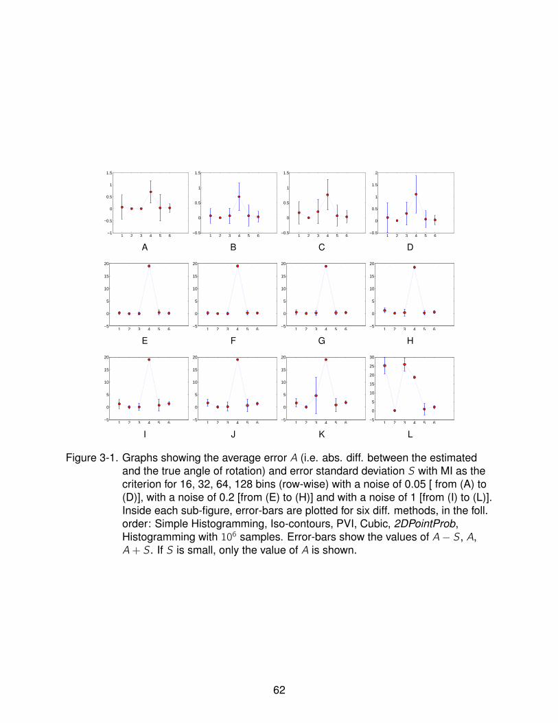
1 2 3 4 5 6−1
−0.5
0
0.5
1
1.5
A1 2 3 4 5 6
−0.5
0
0.5
1
1.5
B1 2 3 4 5 6
−0.5
0
0.5
1
1.5
C1 2 3 4 5 6
−0.5
0
0.5
1
1.5
2
D
1 2 3 4 5 6−5
0
5
10
15
20
E1 2 3 4 5 6
−5
0
5
10
15
20
F1 2 3 4 5 6
−5
0
5
10
15
20
G1 2 3 4 5 6
−5
0
5
10
15
20
H
1 2 3 4 5 6−5
0
5
10
15
20
I1 2 3 4 5 6
−5
0
5
10
15
20
J1 2 3 4 5 6
−5
0
5
10
15
20
K1 2 3 4 5 6
−5
0
5
10
15
20
25
30
L
Figure 3-1. Graphs showing the average error A (i.e. abs. diff. between the estimatedand the true angle of rotation) and error standard deviation S with MI as thecriterion for 16, 32, 64, 128 bins (row-wise) with a noise of 0.05 [ from (A) to(D)], with a noise of 0.2 [from (E) to (H)] and with a noise of 1 [from (I) to (L)].Inside each sub-figure, error-bars are plotted for six diff. methods, in the foll.order: Simple Histogramming, Iso-contours, PVI, Cubic, 2DPointProb,Histogramming with 106 samples. Error-bars show the values of A− S , A,A+ S . If S is small, only the value of A is shown.
62
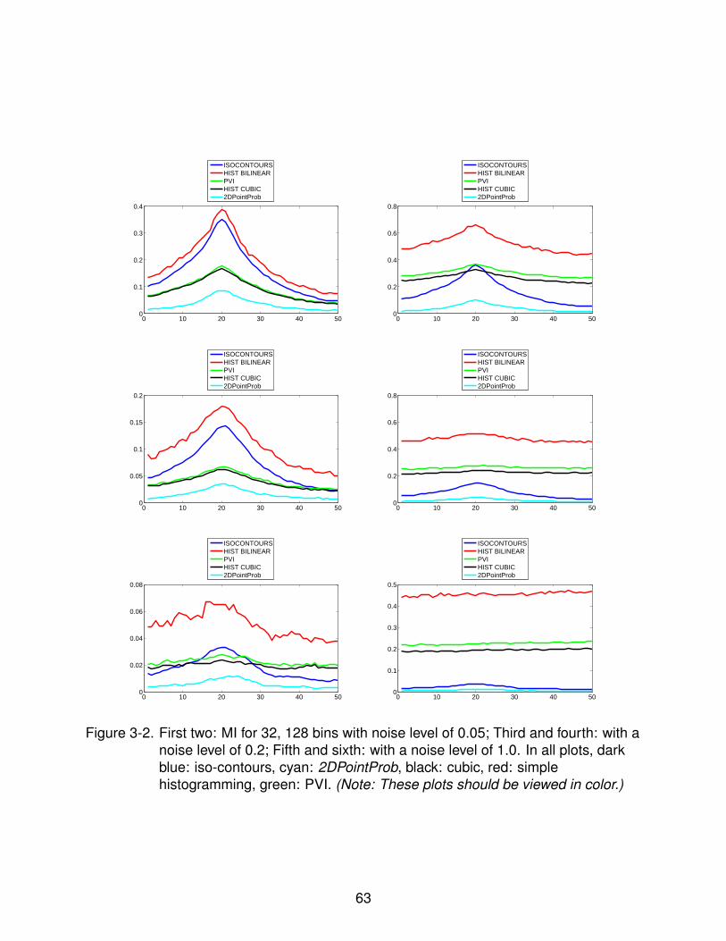
0 10 20 30 40 500
0.1
0.2
0.3
0.4
ISOCONTOURSHIST BILINEARPVIHIST CUBIC2DPointProb
0 10 20 30 40 500
0.2
0.4
0.6
0.8
ISOCONTOURSHIST BILINEARPVIHIST CUBIC2DPointProb
0 10 20 30 40 500
0.05
0.1
0.15
0.2
ISOCONTOURSHIST BILINEARPVIHIST CUBIC2DPointProb
0 10 20 30 40 500
0.2
0.4
0.6
0.8
ISOCONTOURSHIST BILINEARPVIHIST CUBIC2DPointProb
0 10 20 30 40 500
0.02
0.04
0.06
0.08
ISOCONTOURSHIST BILINEARPVIHIST CUBIC2DPointProb
0 10 20 30 40 500
0.1
0.2
0.3
0.4
0.5
ISOCONTOURSHIST BILINEARPVIHIST CUBIC2DPointProb
Figure 3-2. First two: MI for 32, 128 bins with noise level of 0.05; Third and fourth: with anoise level of 0.2; Fifth and sixth: with a noise level of 1.0. In all plots, darkblue: iso-contours, cyan: 2DPointProb, black: cubic, red: simplehistogramming, green: PVI. (Note: These plots should be viewed in color.)
63

A B C
Figure 3-3. MR slices of the brain (A) MR-PD slice, (B) MR-T1 slice rotated by 20degrees, (C) MR-T2 slice rotated by 30 degrees
020
40
0
20
400
1
2
A
020
40
0
20
400
1
2
B
020
40
0
20
401
2
3
4
C
020
40
0
20
400
1
2
3
D
Figure 3-4. MI computed using (A) histogramming and (B) LengthProb (plotted versusθY and θZ ); MMI computed using (C) histogramming and (D) 3DPointProb(plotted versus θ2 and θ3)
64
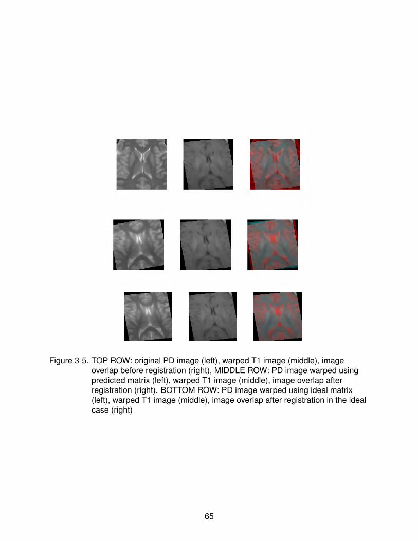
Figure 3-5. TOP ROW: original PD image (left), warped T1 image (middle), imageoverlap before registration (right), MIDDLE ROW: PD image warped usingpredicted matrix (left), warped T1 image (middle), image overlap afterregistration (right). BOTTOM ROW: PD image warped using ideal matrix(left), warped T1 image (middle), image overlap after registration in the idealcase (right)
65

Table 3-2. Average value and variance of parameters θ, s and t predicted by variousmethods (32 and 64 bins, noise σ = 0.2); Ground truth: θ = 30, s = t = −0.3
Method Bins θ s t
MI Hist 32 30, 0 -0.3, 0 -0.3, 0NMI Hist 32 30, 0 -0.3, 0 -0.3, 0MI Iso 32 30, 0 -0.3, 0 -0.3, 0
NMI Iso 32 30, 0 -0.3, 0 -0.3, 0MI PVI 32 30, 0 -0.3, 0 -0.3, 0
NMI PVI 32 30, 0 -0.3, 0 -0.3, 0MI Spline 32 30.8,0.2 -0.3, 0 -0.3, 0
NMI Spline 32 30.6,0.7 -0.3, 0 -0.3, 0MI 2DPt. 32 30, 0 -0.3, 0 -0.3, 0
NMI 2DPt. 32 30, 0 -0.3, 0 -0.3, 0MI Hist 64 29.2,49.7 0.4, 0 0.27, 0.07
NMI Hist 64 28.8,44.9 0.4, 0 0.33, 0.04MI Iso 64 30, 0 -0.3, 0 -0.3,0
NMI Iso 64 30, 0 -0.3, 0 -0.3, 0MI PVI 64 30, 0 -0.3, 0 -0.3, 0
NMI PVI 64 30, 0 -0.3, 0 -0.3, 0MI Spline 64 24,21.5 0.4, 0 0.33, 0.04
NMI Spline 64 24.3,20.9 0.4,0 0.33, 0.04MI 2DPt. 64 30, 0 -0.3, 0 -0.3, 0
NMI 2DPt. 64 30, 0 -0.3, 0 -0.3, 0
66
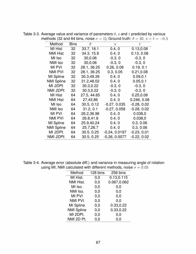
Table 3-3. Average value and variance of parameters θ, s and t predicted by variousmethods (32 and 64 bins, noise σ = 1); Ground truth: θ = 30, s = t = −0.3
Method Bins θ s t
MI Hist 32 33.7, 18.1 0.4, 0 0.13,0.08NMI Hist 32 34.3, 15.9 0.4, 0 0.13, 0.08MI Iso 32 30,0.06 -0.3, 0 -0.3, 0
NMI Iso 32 30,0.06 -0.3, 0 -0.3, 0MI PVI 32 28.1, 36.25 0.26, 0.08 0.19, 0.1
NMI PVI 32 28.1, 36.25 0.3, 0.05 0.21,0.08MI Spline 32 30.3,49.39 0.4, 0 0.09,0.1
NMI Spline 32 31.2,48.02 0.4, 0 0.05,0.1MI 2DPt. 32 30.3,0.22 -0.3, 0 -0.3, 0
NMI 2DPt. 32 30.3,0.22 -0.3, 0 -0.3, 0MI Hist 64 27.5, 44.65 0.4, 0 0.25,0.08
NMI Hist 64 27,43.86 0.4, 0 0.246, 0.08MI Iso 64 30.5, 0.12 -0.27, 0.035 -0.28, 0.02
NMI Iso 64 31.2, 0.1 -0.27, 0.058 -0.28, 0.02MI PVI 64 26.2,36.96 0.4, 0 0.038,0
NMI PVI 64 26.8,41.8 0.4, 0 0.038,0MI Spline 64 25.9,40.24 0.4, 0 0.3, 0.06
NMI Spline 64 25.7,26.7 0.4, 0 0.3, 0.06MI 2DPt. 64 30.5, 0.25 -0.24, 0.0197 -0.23, 0.01
NMI 2DPt. 64 30.5, 0.25 -0.26, 0.0077 -0.22, 0.02
Table 3-4. Average error (absolute diff.) and variance in measuring angle of rotationusing MI, NMI calculated with different methods, noise σ = 0.05
Method 128 bins 256 binsMI Hist. 0,0 0.13,0.115
NMI Hist. 0,0 0.067,0.062MI Iso. 0,0 0,0
NMI Iso. 0,0 0,0MI PVI 0,0 0,0
NMI PVI 0,0 0,0MI Spline 0,0 0.33,0.22
NMI Spline 0,0 0.33,0.22MI 2DPt. 0,0 0,0
NMI 2D Pt. 0,0 0,0
67
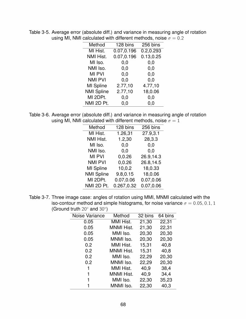
Table 3-5. Average error (absolute diff.) and variance in measuring angle of rotationusing MI, NMI calculated with different methods, noise σ = 0.2
Method 128 bins 256 binsMI Hist. 0.07,0.196 0.2,0.293
NMI Hist. 0.07,0.196 0.13,0.25MI Iso. 0,0 0,0
NMI Iso. 0,0 0,0MI PVI 0,0 0,0
NMI PVI 0,0 0,0MI Spline 2.77,10 4.77,10
NMI Spline 2.77,10 18,0.06MI 2DPt. 0,0 0,0
NMI 2D Pt. 0,0 0,0
Table 3-6. Average error (absolute diff.) and variance in measuring angle of rotationusing MI, NMI calculated with different methods, noise σ = 1
Method 128 bins 256 binsMI Hist. 1.26,31 27.9,3.1
NMI Hist. 1.2,30 28,3.3MI Iso. 0,0 0,0
NMI Iso. 0,0 0,0MI PVI 0,0.26 26.9,14.3
NMI PVI 0,0.26 26.8,14.5MI Spline 10,0.2 18,0.33
NMI Spline 9.8,0.15 18,0.06MI 2DPt. 0.07,0.06 0.07,0.06
NMI 2D Pt. 0.267,0.32 0.07,0.06
Table 3-7. Three image case: angles of rotation using MMI, MNMI calculated with theiso-contour method and simple histograms, for noise variance σ = 0.05, 0.1, 1(Ground truth 20 and 30)
Noise Variance Method 32 bins 64 bins0.05 MMI Hist. 21,30 22,310.05 MNMI Hist. 21,30 22,310.05 MMI Iso. 20,30 20,300.05 MNMI Iso. 20,30 20,300.2 MMI Hist. 15,31 40,80.2 MNMI Hist. 15,31 40,80.2 MMI Iso. 22,29 20,300.2 MNMI Iso. 22,29 20,301 MMI Hist. 40,9 38,41 MNMI Hist. 40,9 34,41 MMI Iso. 22,30 35,231 MNMI Iso. 22,30 40,3
68
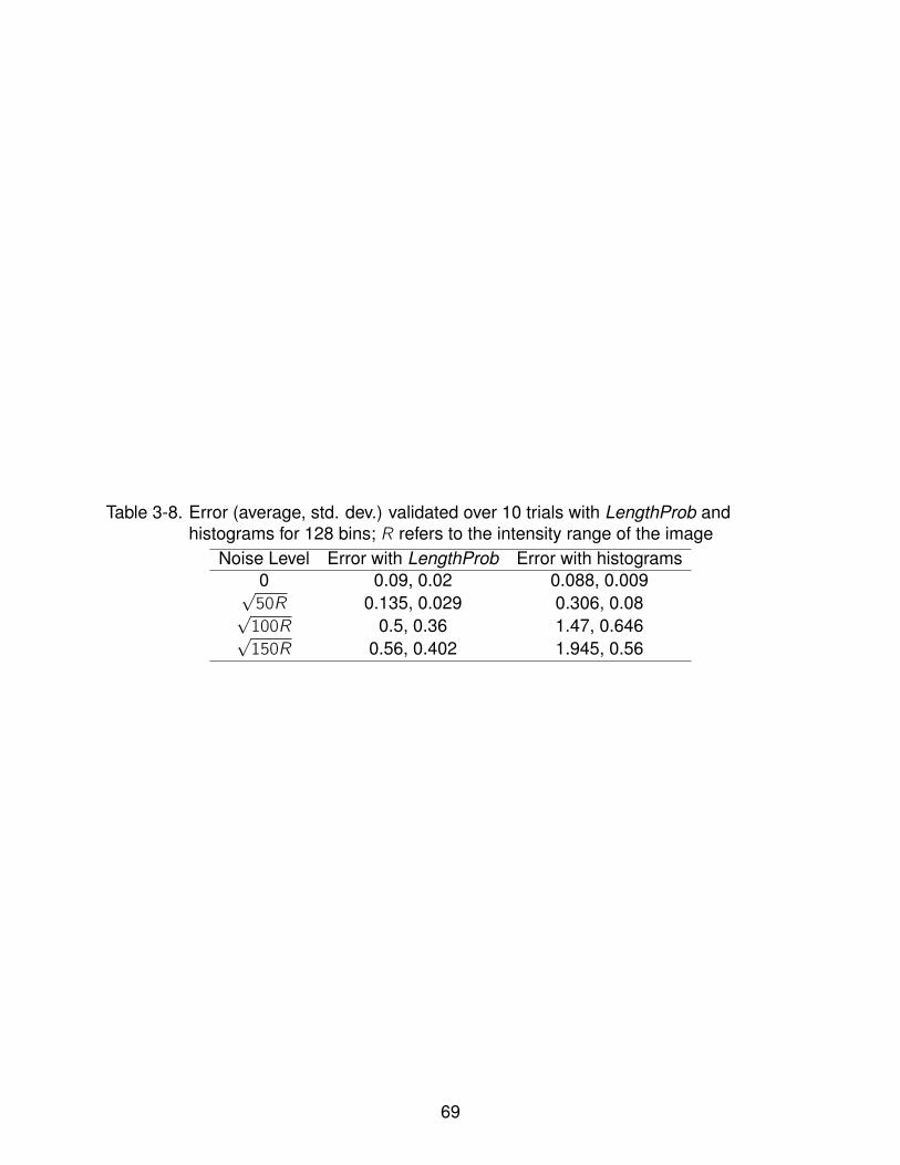
Table 3-8. Error (average, std. dev.) validated over 10 trials with LengthProb andhistograms for 128 bins; R refers to the intensity range of the image
Noise Level Error with LengthProb Error with histograms0 0.09, 0.02 0.088, 0.009√50R 0.135, 0.029 0.306, 0.08√100R 0.5, 0.36 1.47, 0.646√150R 0.56, 0.402 1.945, 0.56
69
CHAPTER 4APPLICATION TO IMAGE FILTERING
4.1 Introduction
Filtering of images has been one of the most fundamental problems studied in
low-level vision and signal processing. Over the past decades, several techniques for
data filtering have been proposed with impressive results on practical applications
in image processing. As straightforward image smoothing is known to blur across
significant image structures, several anisotropic approaches to image smoothing have
been developed using partial differential equations (PDEs) with stopping terms to
control image diffusion in different directions [44]. The PDE-based approaches have
been extended to filtering of color images [45] and chromaticity vector fields [46]. Other
popular approaches to image filtering include adaptive smoothing [47] and kernel
density estimation based algorithms [48]. All these methods produce some sort of
weighted average over an image neighborhood for the purpose of data smoothing,
where the weights are obtained from the difference between the intensity values of the
central pixel and the pixels in the neighborhood, or from the pixel gradient magnitudes.
Beyond this, techniques such as bilateral filtering [49] produce a weighted combination
that is also influenced by the relative location of the central pixel and the neighborhood
pixels. The highly popular mean-shift procedure [50], [51] is grounded in similar ideas
as bilateral filtering, with the addition that the neighborhood around a pixel is allowed
to change dynamically until a convergence criterion is met. The authors prove that this
convergence criterion is equivalent to finding the mode of a local density built jointly on
the spatial parameters (image domain) and the intensity parameters (image range).
In this chapter, we present a new approach to data filtering that is rooted in simple
yet elegant geometric intuitions. At the core of our theory is the representation of an
image as a function that is at least C0 continuous everywhere. A key property of the
image level sets is used to drive the diffusion process, which we then incorporate in a
70
framework of dynamic neighborhoods a la mean-shift. We demonstrate the relationship
of our method to many of the existing filtering techniques such as those driven by
kernel density estimation. The efficacy of our approach is supported with extensive
experimental results. To the best of our knowledge, ours is the first attempt to explicitly
utilize image geometry (in terms of its level curves) for this particular application.
This chapter is organized as follows. Section 2 presents the key theoretical
framework. Section 3 presents extensions to our theory. In section 4, we present
the relationship between our method and mean-shift. Extensive experimental results are
presented in section 5, and we present further discussions and conclusions in section 6.
All or most of the material contained in this chapter has been previously published by the
author in [52]1 .
4.2 Theory
Consider an image over a discrete domain Ω = 1, ...,H × 1, ...,W where
the intensity of each discrete location (x , y) is given by I (x , y). Moreover consider
a neighborhood N (xi , yi) around the pixel (xi , yi). It is well-known that a simple
averaging of all intensity values in N (xi , yi) will blur edges, so a weighted combination is
calculated, where the weight of the j th pixel is given by w (1)(xj , yj) = g(|I (xi , yi)−I (xj , yj)|)
for a non-increasing function g(.) to facilitate anisotropic diffusion, with common
examples being g(z) = e−z2
σ2 or g(z) = σ2
σ2+z2, or their truncated versions. This approach
is akin to the kernel density estimation (KDE) approach proposed in [48], where the
1 Parts of the content of this chapter have been reprinted with permission from: A.Rajwade, A. Banerjee and A. Rangarajan, ‘Image Filtering by Level Curves’, EnergyMinimization Methods in Computer Vision and Pattern Recognition (EMMCVPR), 2009,pages 359-372. c©2009, Springer Verlag.
71
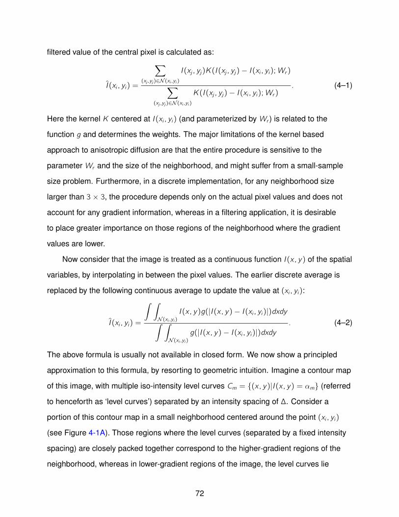
filtered value of the central pixel is calculated as:
I (xi , yi) =
∑(xj ,yj )∈N (xi ,yi )
I (xj , yj)K(I (xj , yj)− I (xi , yi);Wr)∑(xj ,yj )∈N (xi ,yi )
K(I (xj , yj)− I (xi , yi);Wr). (4–1)
Here the kernel K centered at I (xi , yi) (and parameterized byWr ) is related to the
function g and determines the weights. The major limitations of the kernel based
approach to anisotropic diffusion are that the entire procedure is sensitive to the
parameterWr and the size of the neighborhood, and might suffer from a small-sample
size problem. Furthermore, in a discrete implementation, for any neighborhood size
larger than 3 × 3, the procedure depends only on the actual pixel values and does not
account for any gradient information, whereas in a filtering application, it is desirable
to place greater importance on those regions of the neighborhood where the gradient
values are lower.
Now consider that the image is treated as a continuous function I (x , y) of the spatial
variables, by interpolating in between the pixel values. The earlier discrete average is
replaced by the following continuous average to update the value at (xi , yi):
I (xi , yi) =
∫ ∫N (xi ,yi )
I (x , y)g(|I (x , y)− I (xi , yi)|)dxdy∫ ∫N (xi ,yi )
g(|I (x , y)− I (xi , yi)|)dxdy. (4–2)
The above formula is usually not available in closed form. We now show a principled
approximation to this formula, by resorting to geometric intuition. Imagine a contour map
of this image, with multiple iso-intensity level curves Cm = (x , y)|I (x , y) = αm (referred
to henceforth as ‘level curves’) separated by an intensity spacing of ∆. Consider a
portion of this contour map in a small neighborhood centered around the point (xi , yi)
(see Figure 4-1A). Those regions where the level curves (separated by a fixed intensity
spacing) are closely packed together correspond to the higher-gradient regions of the
neighborhood, whereas in lower-gradient regions of the image, the level curves lie
72
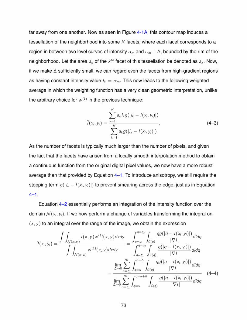
far away from one another. Now as seen in Figure 4-1A, this contour map induces a
tessellation of the neighborhood into some K facets, where each facet corresponds to a
region in between two level curves of intensity αm and αm + ∆, bounded by the rim of the
neighborhood. Let the area ak of the k th facet of this tessellation be denoted as ak . Now,
if we make ∆ sufficiently small, we can regard even the facets from high-gradient regions
as having constant intensity value Ik = αm. This now leads to the following weighted
average in which the weighting function has a very clean geometric interpretation, unlike
the arbitrary choice for w (1) in the previous technique:
I (xi , yi) =
K∑k=1
ak Ikg(|Ik − I (xi , yi)|)
K∑k=1
akg(|Ik − I (xi , yi)|). (4–3)
As the number of facets is typically much larger than the number of pixels, and given
the fact that the facets have arisen from a locally smooth interpolation method to obtain
a continuous function from the original digital pixel values, we now have a more robust
average than that provided by Equation 4–1. To introduce anisotropy, we still require the
stopping term g(|Ik − I (xi , yi)|) to prevent smearing across the edge, just as in Equation
4–1.
Equation 4–2 essentially performs an integration of the intensity function over the
domain N (xi , yi). If we now perform a change of variables transforming the integral on
(x , y) to an integral over the range of the image, we obtain the expression
I (xi , yi) =
∫ ∫N (xi ,yi )
I (x , y)w (1)(x , y)dxdy∫ ∫N (xi ,yi )
w (1)(x , y)dxdy
=
∫ q=q2q=q1
∫C(q)
qg(|q − I (xi , yi)|)|∇I |
dldq∫ q=q2q=q1
∫C(q)
g(|q − I (xi , yi)|)|∇I |
dldq
=
lim∆→0
q2∑α=q1
∫ α+∆
q=α
∫C(q)
qg(|q − I (xi , yi)|)|∇I |
dldq
lim∆→0
q2∑α=q1
∫ q=α+∆q=α
∫C(q)
g(|q − I (xi , yi)|)|∇I |
dldq
(4–4)
73
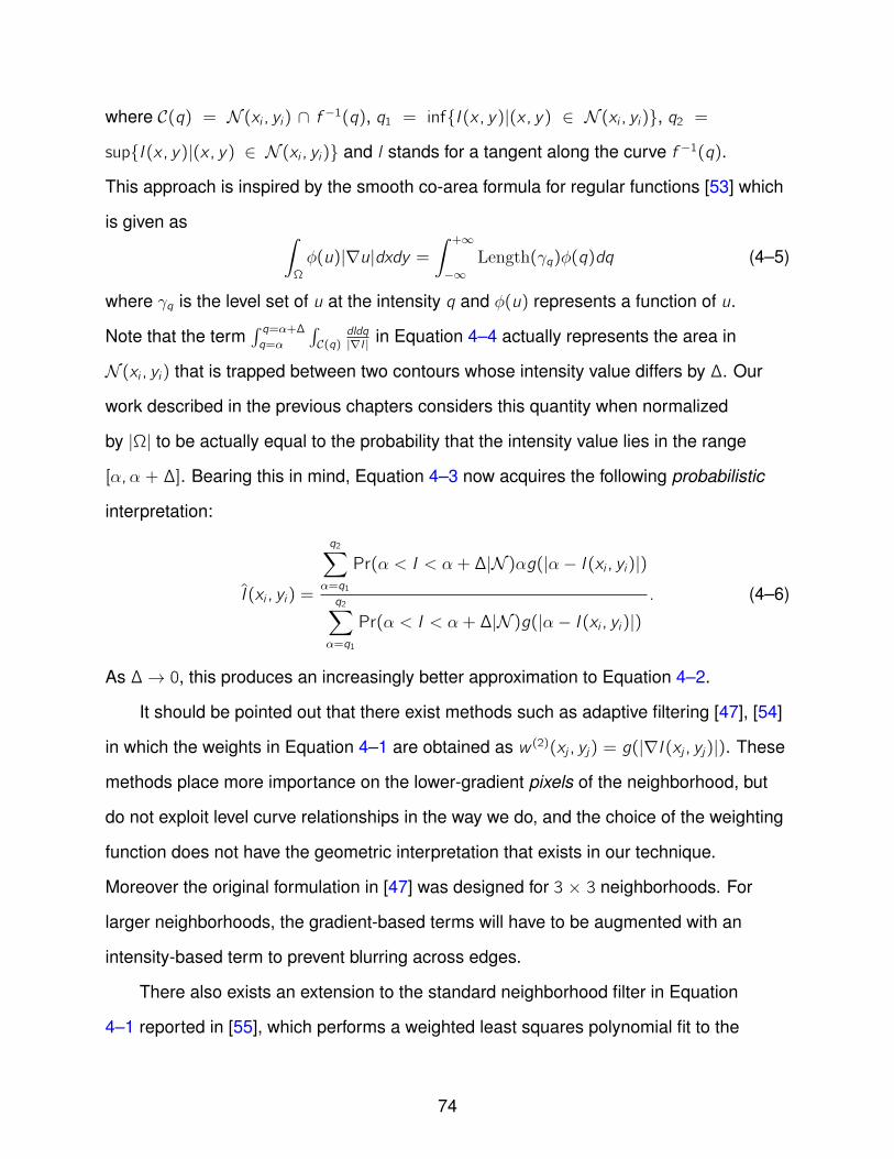
where C(q) = N (xi , yi) ∩ f −1(q), q1 = infI (x , y)|(x , y) ∈ N (xi , yi), q2 =
supI (x , y)|(x , y) ∈ N (xi , yi) and l stands for a tangent along the curve f −1(q).
This approach is inspired by the smooth co-area formula for regular functions [53] which
is given as ∫Ω
φ(u)|∇u|dxdy =∫ +∞−∞
Length(γq)φ(q)dq (4–5)
where γq is the level set of u at the intensity q and φ(u) represents a function of u.
Note that the term∫ q=α+∆q=α
∫C(q)
dldq|∇I | in Equation 4–4 actually represents the area in
N (xi , yi) that is trapped between two contours whose intensity value differs by ∆. Our
work described in the previous chapters considers this quantity when normalized
by |Ω| to be actually equal to the probability that the intensity value lies in the range
[α,α + ∆]. Bearing this in mind, Equation 4–3 now acquires the following probabilistic
interpretation:
I (xi , yi) =
q2∑α=q1
Pr(α < I < α+ ∆|N )αg(|α− I (xi , yi)|)
q2∑α=q1
Pr(α < I < α+ ∆|N )g(|α− I (xi , yi)|). (4–6)
As ∆→ 0, this produces an increasingly better approximation to Equation 4–2.
It should be pointed out that there exist methods such as adaptive filtering [47], [54]
in which the weights in Equation 4–1 are obtained as w (2)(xj , yj) = g(|∇I (xj , yj)|). These
methods place more importance on the lower-gradient pixels of the neighborhood, but
do not exploit level curve relationships in the way we do, and the choice of the weighting
function does not have the geometric interpretation that exists in our technique.
Moreover the original formulation in [47] was designed for 3 × 3 neighborhoods. For
larger neighborhoods, the gradient-based terms will have to be augmented with an
intensity-based term to prevent blurring across edges.
There also exists an extension to the standard neighborhood filter in Equation
4–1 reported in [55], which performs a weighted least squares polynomial fit to the
74
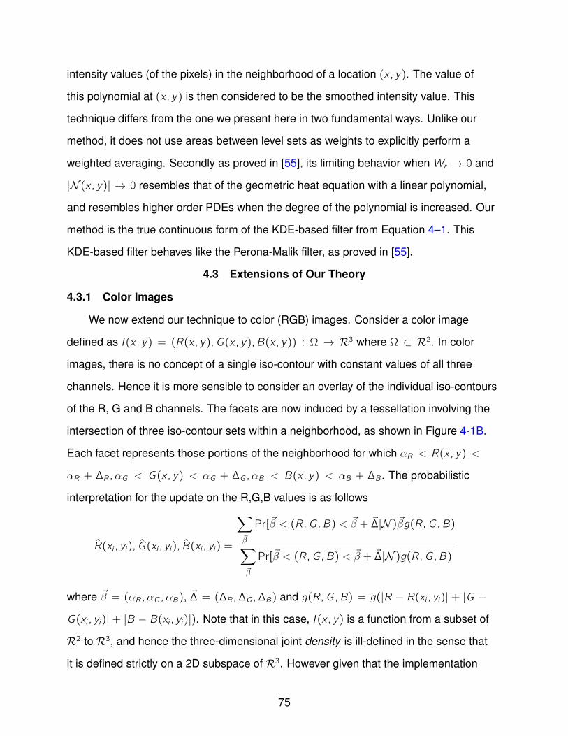
intensity values (of the pixels) in the neighborhood of a location (x , y). The value of
this polynomial at (x , y) is then considered to be the smoothed intensity value. This
technique differs from the one we present here in two fundamental ways. Unlike our
method, it does not use areas between level sets as weights to explicitly perform a
weighted averaging. Secondly as proved in [55], its limiting behavior whenWr → 0 and
|N (x , y)| → 0 resembles that of the geometric heat equation with a linear polynomial,
and resembles higher order PDEs when the degree of the polynomial is increased. Our
method is the true continuous form of the KDE-based filter from Equation 4–1. This
KDE-based filter behaves like the Perona-Malik filter, as proved in [55].
4.3 Extensions of Our Theory
4.3.1 Color Images
We now extend our technique to color (RGB) images. Consider a color image
defined as I (x , y) = (R(x , y),G(x , y),B(x , y)) : Ω → R3 where Ω ⊂ R2. In color
images, there is no concept of a single iso-contour with constant values of all three
channels. Hence it is more sensible to consider an overlay of the individual iso-contours
of the R, G and B channels. The facets are now induced by a tessellation involving the
intersection of three iso-contour sets within a neighborhood, as shown in Figure 4-1B.
Each facet represents those portions of the neighborhood for which αR < R(x , y) <
αR + ∆R ,αG < G(x , y) < αG + ∆G ,αB < B(x , y) < αB + ∆B . The probabilistic
interpretation for the update on the R,G,B values is as follows
R(xi , yi), G(xi , yi), B(xi , yi) =
∑~β
Pr[~β < (R,G ,B) < ~β + ~∆|N )~βg(R,G ,B)
∑~β
Pr[~β < (R,G ,B) < ~β + ~∆|N )g(R,G ,B)
where ~β = (αR ,αG ,αB), ~∆ = (∆R , ∆G , ∆B) and g(R,G ,B) = g(|R − R(xi , yi)| + |G −
G(xi , yi)| + |B − B(xi , yi)|). Note that in this case, I (x , y) is a function from a subset of
R2 to R3, and hence the three-dimensional joint density is ill-defined in the sense that
it is defined strictly on a 2D subspace of R3. However given that the implementation
75
considers joint cumulative interval measures, this does not pose any problem in a
practical implementation. We wish to emphasize that the averaging of the R,G,B values
is performed in a strictly coupled manner, all affected by the joint cumulative interval
measure.
4.3.2 Chromaticity Fields
Previous research on filtering chromaticity noise (which affects only the direction
and not the magnitude of the RGB values at image pixels) includes the work in [46]
using PDEs specially tuned for unit-vector data, and the work in [48] (page 142) using
kernel density estimation for directional data. The more recent work on chromaticity
filtering in [56] actually treats chromaticity vectors as points on a Grassmann manifold
G1,3 as opposed to treating them as points on S2, which is the approach presented here
and in [48] and [46].
We extend our theory from the previous section to unit vector data and incorporate
it in a mean-shift framework for smoothing. Let I (x , y) : Ω → R3 be the original
RGB image, and let J(x , y) : Ω → S2 be the corresponding field of chromaticity
vectors. A possible approach would involve interpolating the chromaticity vectors
by means of commonly used spherical interpolants to create a continuous function,
followed by tracing the level curves of the individual unit-vector components ~v(x , y) =
(v1(x , y), v2(x , y), v3(x , y)) and computing their intersection. However for ease of
implementation for this particular application, we resorted to a different strategy. If the
intensity intervals ~∆ = (∆R , ∆G , ∆B) are chosen to be fine enough, then each facet
induced by a tessellation that uses the level curves of the R, G and B channel values,
can be regarded as having a constant color value, and hence the chromaticity vector
values within that facet can be regarded as (almost) constant. Therefore it is possible
to use just the R,G,B level curves for the task of chromaticity smoothing as well. The
update equation is very similar to Equation 4–7 with the R,G,B vectors replaced by their
unit normalized versions. However as the averaging process does not preserve the unit
76

norm, the averaged vector needs to be renormalized to produce the spherical weighted
mean.
4.3.3 Gray-scale Video
For the purpose of this application, the video is treated as a single 3D signal
(volume). The extension in this case is quite straightforward, with the areas between
level curves being replaced by volumes between the level surfaces at nearby intensities.
However we take into account the causality factor in defining the temporal component of
the neighborhood around a pixel, by performing the averaging at each pixel over frames
only from the past.
4.4 Level Curve Based Filtering in a Mean Shift Framework
All the above techniques are based on an averaging operation over only the image
intensities (i.e. in the range domain). On the other hand, techniques such as bilateral
filtering [49] or local mode-finding [57] combine both range and spatial domain, thus
using weights of the form wj = g(s)((xi − xj)2 + (yi − yj)2)g(r)(|(I (xi , yi) − I (xj , yj)|) in
Equation 4–1, where g(s) and g(r) affect the spatial and range kernels respectively. The
mean-shift framework [51] is based on similar principles, but changes the filter window
dynamically for several iterations until it finds a local mode of the joint density of the
spatial and range parameters, estimated using kernels based on the functions g(r) and
g(s). Our level curve based approach fits easily into this framework with the addition
of a spatial kernel. One way to do this would be to consider the image as a surface
embedded in 3D (a Monge patch), as done in [58], and compute areas of patches in
3D for the probability values. However such an approach may not necessarily favor
the lower gradient areas of the image. Instead we adopt another method wherein we
assume two additional functions of x and y , namely X (x , y) = x and Y (x , y) = y . We
compute the joint probabilities for a range of values of the joint variable (X ,Y , I ) by
drawing local level sets and computing areas in 2D. Assuming a uniform spatial kernel
for g(s) within a radiusWs and a rectangular kernel on the intensity for g(r) with threshold
77
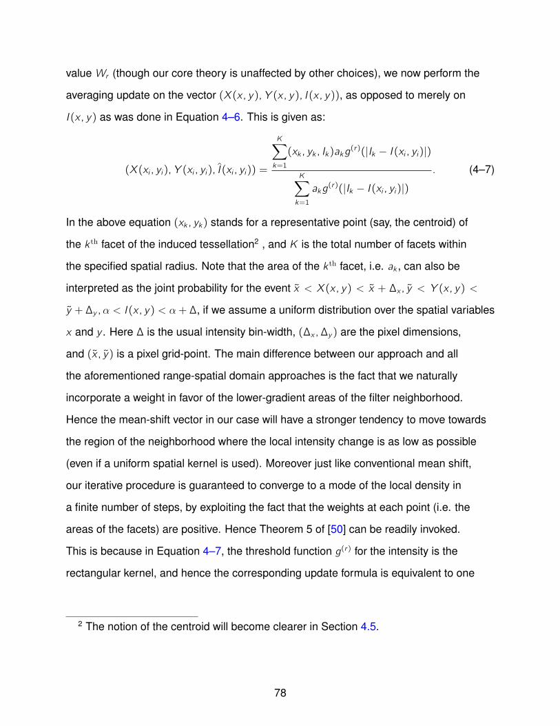
valueWr (though our core theory is unaffected by other choices), we now perform the
averaging update on the vector (X (x , y),Y (x , y), I (x , y)), as opposed to merely on
I (x , y) as was done in Equation 4–6. This is given as:
(X (xi , yi),Y (xi , yi), I (xi , yi)) =
K∑k=1
(xk , yk , Ik)akg(r)(|Ik − I (xi , yi)|)
K∑k=1
akg(r)(|Ik − I (xi , yi)|)
. (4–7)
In the above equation (xk , yk) stands for a representative point (say, the centroid) of
the k th facet of the induced tessellation2 , and K is the total number of facets within
the specified spatial radius. Note that the area of the k th facet, i.e. ak , can also be
interpreted as the joint probability for the event x < X (x , y) < x + ∆x , y < Y (x , y) <
y +∆y ,α < I (x , y) < α+∆, if we assume a uniform distribution over the spatial variables
x and y . Here ∆ is the usual intensity bin-width, (∆x , ∆y) are the pixel dimensions,
and (x , y) is a pixel grid-point. The main difference between our approach and all
the aforementioned range-spatial domain approaches is the fact that we naturally
incorporate a weight in favor of the lower-gradient areas of the filter neighborhood.
Hence the mean-shift vector in our case will have a stronger tendency to move towards
the region of the neighborhood where the local intensity change is as low as possible
(even if a uniform spatial kernel is used). Moreover just like conventional mean shift,
our iterative procedure is guaranteed to converge to a mode of the local density in
a finite number of steps, by exploiting the fact that the weights at each point (i.e. the
areas of the facets) are positive. Hence Theorem 5 of [50] can be readily invoked.
This is because in Equation 4–7, the threshold function g(r) for the intensity is the
rectangular kernel, and hence the corresponding update formula is equivalent to one
2 The notion of the centroid will become clearer in Section 4.5.
78
with a weighted rectangular kernel, with the weights being determined by the areas of
the facets.
A major advantage of our technique is that the parameter ∆ can be set to as small
a value as desired (as it just means that more and more level curves are being used),
and the interpolation gives rise to a robust average. This is especially useful in the case
of small neighborhood sizes, as the intensity quantization is now no more limited by the
number of available pixels. In conventional mean-shift, the proper choice of bandwidth
is a highly critical issue, as very few samples are available for the local density estimate.
Though variable bandwidth procedures for mean-shift algorithms have been developed
extensively, they themselves require either the tuning of other parameters using rules of
thumb, or else some expensive exhaustive searches for the automatic determination of
the bandwidth [59], [60]. Although our method does require the selection ofWs andWr ,
the filtering results are less sensitive to the choice of these parameters in our method
than in standard mean shift.
4.5 Experimental Results
In this section we present experimental results to compare the performance of our
algorithm in a mean shift framework w.r.t. conventional kernel-based mean shift. For our
algorithm, we obtain a continuous function approximation to the digital image, by means
of piecewise linear interpolants fit to a triple of intensity values in half-pixels of the image
(in principle, we could have used any other smooth interpolant). The corresponding level
sets for such a function are also very easy to trace, as they are just segments within
each half-pixel. The level sets induce a polygonal tessellation. We choose to split the
polygons by the square pixel boundaries as well as the pixel diagonals that delineate the
half-pixel boundaries, thereby convexifying all the polygons that were initially non-convex
(see Figure 4-1C). Each polygon in the tessellation can now be characterized by the x , y
coordinates of its centroid, the intensity value of the image at the centroid, and the area
of the polygon. Thus, if the intensity value at grid location xi , yi is to be smoothed, we
79
choose a window of spatial radiusWs and intensity radiusWr around (xi , yi , I (xi , yi)),
over which the averaging is performed. In other words, the averaging is performed only
over those locations x , y for which (x − xi)2+(y − yi)2 <W 2s and |I (x , y)− I (xi , yi)| <Wr .
We would like to point out that though the interpolant used for creating the continuous
image representation is indeed isotropic in nature, this still does not make our filtering
algorithm isotropic. This is because polygonal regions, whose intensity value does not
satisfy the constraint |I (x , y)− I (xi , yi)| < Wr , do not contribute to the averaging process
(see the stopping term in Equation 4–3), and hence the contribution from pixels with
very different intensity values will be nullified.
4.5.1 Gray-scale Images
We ran our filtering algorithm over four arbitrarily chosen images from the popular
Berkeley image dataset [61], and the Lena image. To all these images, zero mean
Gaussian noise of variance 0.003 (per unit gray-scale range) was added. The filtering
was performed usingWs = Wr = 3 for our algorithm and compared to mean-shift
using Gaussian and Epanechnikov kernels with the same parameter. Our method
produced superior filtering results to conventional mean shift with both Gaussian and
Epanechnikov kernels. The results for our method and for Gaussian kernel mean shift
are displayed in Figures 4-2 and 4-3 respectively. The visually superior appearance
was confirmed objectively with mean squared error (MSE) values in Table 4-1. It should
be noted that the aim was to compare our method to standard mean shift for the exact
same setting of the parametersWr andWs , as they have the same meaning in all these
algorithms. Although increasing the value ofWr will provide more samples for averaging,
this will allow more and more intensity values to leak across edges.
4.5.2 Testing on a Benchmark Dataset of Gray-scale Images
Further empirical results with our algorithm (usingWS = Wr = 5) were obtained
on Lansel’s benchmark dataset [62]. The dataset contains noisy versions of 13 different
images. Each noisy image is obtained from one of three noise models: additive
80
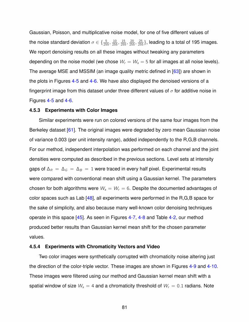
Gaussian, Poisson, and multiplicative noise model, for one of five different values of
the noise standard deviation σ ∈ 5255, 10255, 15255, 20255, 25255
, leading to a total of 195 images.
We report denoising results on all these images without tweaking any parameters
depending on the noise model (we choseWr =Ws = 5 for all images at all noise levels).
The average MSE and MSSIM (an image quality metric defined in [63]) are shown in
the plots in Figures 4-5 and 4-6. We have also displayed the denoised versions of a
fingerprint image from this dataset under three different values of σ for additive noise in
Figures 4-5 and 4-6.
4.5.3 Experiments with Color Images
Similar experiments were run on colored versions of the same four images from the
Berkeley dataset [61]. The original images were degraded by zero mean Gaussian noise
of variance 0.003 (per unit intensity range), added independently to the R,G,B channels.
For our method, independent interpolation was performed on each channel and the joint
densities were computed as described in the previous sections. Level sets at intensity
gaps of ∆R = ∆G = ∆B = 1 were traced in every half pixel. Experimental results
were compared with conventional mean shift using a Gaussian kernel. The parameters
chosen for both algorithms wereWs = Wr = 6. Despite the documented advantages of
color spaces such as Lab [48], all experiments were performed in the R,G,B space for
the sake of simplicity, and also because many well-known color denoising techniques
operate in this space [45]. As seen in Figures 4-7, 4-8 and Table 4-2, our method
produced better results than Gaussian kernel mean shift for the chosen parameter
values.
4.5.4 Experiments with Chromaticity Vectors and Video
Two color images were synthetically corrupted with chromaticity noise altering just
the direction of the color-triple vector. These images are shown in Figures 4-9 and 4-10.
These images were filtered using our method and Gaussian kernel mean shift with a
spatial window of sizeWs = 4 and a chromaticity threshold ofWr = 0.1 radians. Note
81
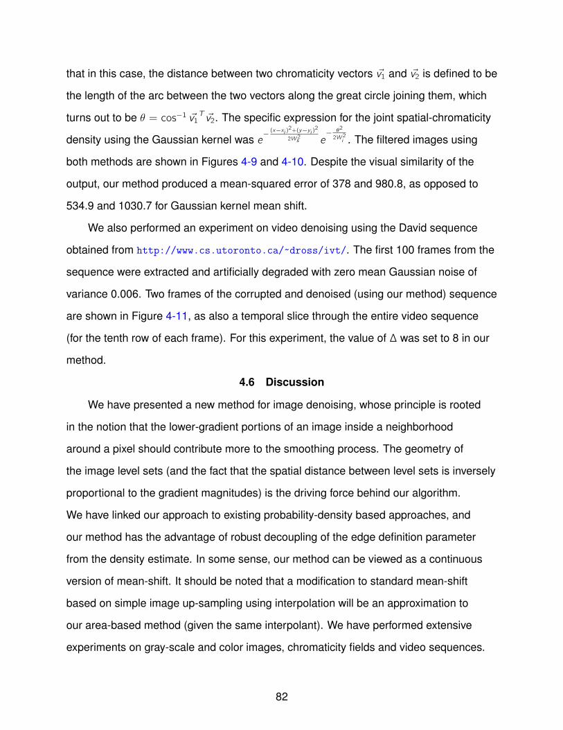
that in this case, the distance between two chromaticity vectors ~v1 and ~v2 is defined to be
the length of the arc between the two vectors along the great circle joining them, which
turns out to be θ = cos−1 ~v1T ~v2. The specific expression for the joint spatial-chromaticity
density using the Gaussian kernel was e− (x−xi )
2+(y−yi )2
2W2s e− θ2
2W2i . The filtered images using
both methods are shown in Figures 4-9 and 4-10. Despite the visual similarity of the
output, our method produced a mean-squared error of 378 and 980.8, as opposed to
534.9 and 1030.7 for Gaussian kernel mean shift.
We also performed an experiment on video denoising using the David sequence
obtained from http://www.cs.utoronto.ca/~dross/ivt/. The first 100 frames from the
sequence were extracted and artificially degraded with zero mean Gaussian noise of
variance 0.006. Two frames of the corrupted and denoised (using our method) sequence
are shown in Figure 4-11, as also a temporal slice through the entire video sequence
(for the tenth row of each frame). For this experiment, the value of ∆ was set to 8 in our
method.
4.6 Discussion
We have presented a new method for image denoising, whose principle is rooted
in the notion that the lower-gradient portions of an image inside a neighborhood
around a pixel should contribute more to the smoothing process. The geometry of
the image level sets (and the fact that the spatial distance between level sets is inversely
proportional to the gradient magnitudes) is the driving force behind our algorithm.
We have linked our approach to existing probability-density based approaches, and
our method has the advantage of robust decoupling of the edge definition parameter
from the density estimate. In some sense, our method can be viewed as a continuous
version of mean-shift. It should be noted that a modification to standard mean-shift
based on simple image up-sampling using interpolation will be an approximation to
our area-based method (given the same interpolant). We have performed extensive
experiments on gray-scale and color images, chromaticity fields and video sequences.
82

To the best of our knowledge, ours is the first piece of work on denoising which explicitly
incorporates the relationship between image level curves and uses local interpo-
lation between pixel values in order to perform filtering. Future work will involve a
more detailed investigation into the relationship between our work and that in [58], by
computing the areas of the contributing regions with explicit treatment of the image
I (x , y) as a surface embedded in 3D. Secondly, we also plan to develop topologically
inspired criteria to automate the choice of the spatial neighborhood and the parameter
Wr for controlling the anisotropic smoothing.
It should be noted that the main aim of this chapter was to demonstrate the effect
of using interpolant information for denoising. Our contributions lie within the mean
shift framework, and therefore we have performed comparisons with other methods
that lie within this framework. For this reason, we have not performed experimental
comparisons with some leading local convolution approaches like [64] or [65].
LOW GRADIENTREGION (LARGE GAP BETWEENLEVEL SETS)
HIGHER GRADIENT REGION(LEVEL SETS CLOSELY PACKED)
CENTRAL PIXEL
A B
FACETS INDUCED BY LEVEL CURVES AND PIXEL GRID
C
Figure 4-1. Image contour maps in a neighborhood (A) with high and low gradientregions in a neighborhood around a pixel (dark dot); (B) a contour map of anRGB image in a neighborhood; red, green and blue contours correspond tocontours of the R,G,B channels respectively and the tessellation induced bythe above level-curve pairs contains 19 facets; (C) A tessellation induced byRGB level curve pairs and the square pixel grid
83
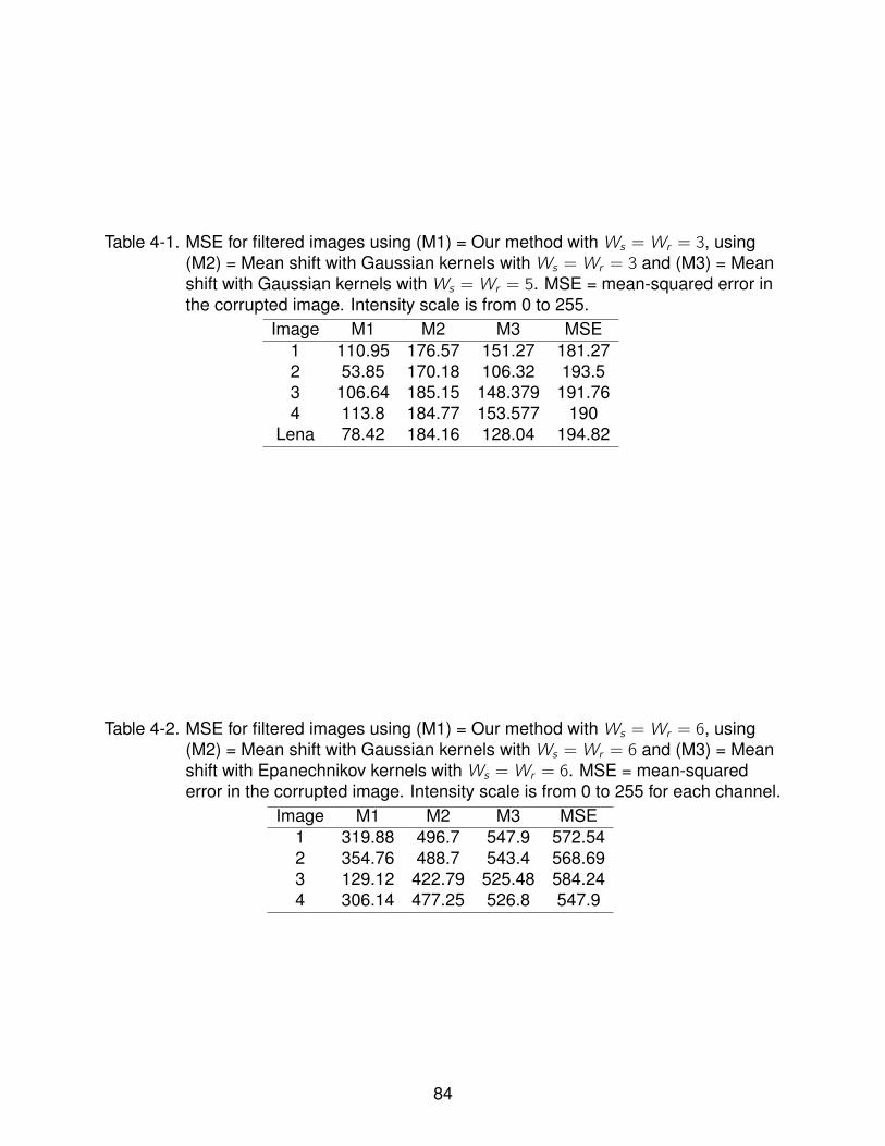
Table 4-1. MSE for filtered images using (M1) = Our method withWs =Wr = 3, using(M2) = Mean shift with Gaussian kernels withWs =Wr = 3 and (M3) = Meanshift with Gaussian kernels withWs =Wr = 5. MSE = mean-squared error inthe corrupted image. Intensity scale is from 0 to 255.
Image M1 M2 M3 MSE1 110.95 176.57 151.27 181.272 53.85 170.18 106.32 193.53 106.64 185.15 148.379 191.764 113.8 184.77 153.577 190
Lena 78.42 184.16 128.04 194.82
Table 4-2. MSE for filtered images using (M1) = Our method withWs =Wr = 6, using(M2) = Mean shift with Gaussian kernels withWs =Wr = 6 and (M3) = Meanshift with Epanechnikov kernels withWs =Wr = 6. MSE = mean-squarederror in the corrupted image. Intensity scale is from 0 to 255 for each channel.
Image M1 M2 M3 MSE1 319.88 496.7 547.9 572.542 354.76 488.7 543.4 568.693 129.12 422.79 525.48 584.244 306.14 477.25 526.8 547.9
84
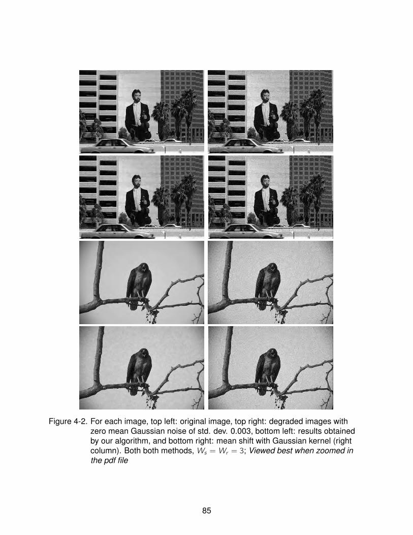
Figure 4-2. For each image, top left: original image, top right: degraded images withzero mean Gaussian noise of std. dev. 0.003, bottom left: results obtainedby our algorithm, and bottom right: mean shift with Gaussian kernel (rightcolumn). Both both methods,Ws =Wr = 3; Viewed best when zoomed inthe pdf file
85

Figure 4-3. For each image, top left: original image, top right: degraded images withzero mean Gaussian noise of std. dev. 0.003, bottom left: results obtainedby our algorithm, and bottom right: mean shift with Gaussian kernel (rightcolumn). Both both methods,Ws =Wr = 3; Viewed best when zoomed inthe pdf file
86

Figure 4-4. Top left: original image, top right: degraded images with zero meanGaussian noise of std. dev. 0.003, bottom left: results obtained by ouralgorithm, and bottom right: mean shift with Gaussian kernel (right column).Both both methods,Ws =Wr = 3; Viewed best when zoomed in the pdf file
87
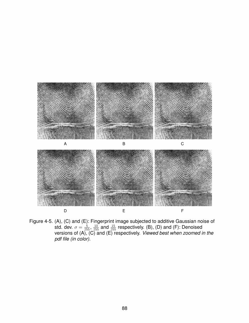
A B C
D E F
Figure 4-5. (A), (C) and (E): Fingerprint image subjected to additive Gaussian noise ofstd. dev. σ = 5
255, 10255
and 15255
respectively. (B), (D) and (F): Denoisedversions of (A), (C) and (E) respectively. Viewed best when zoomed in thepdf file (in color).
88
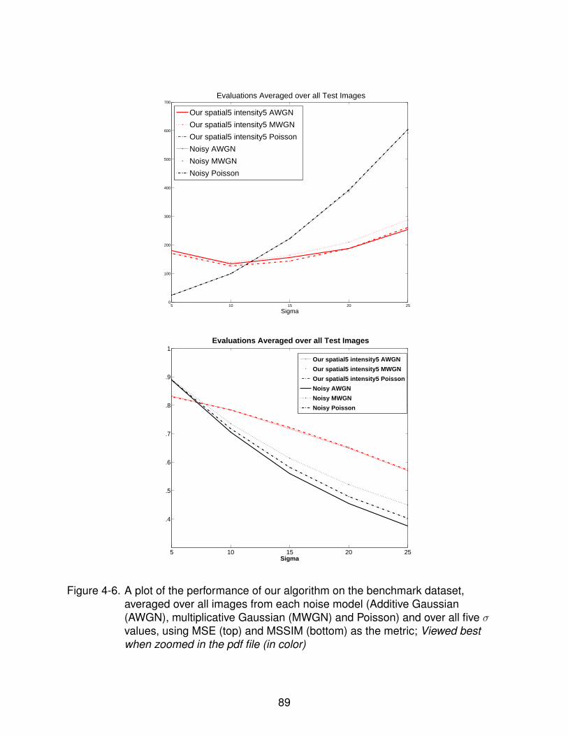
5 10 15 20 250
100
200
300
400
500
600
700
Sigma
Evaluations Averaged over all Test Images
Our spatial5 intensity5 AWGN
Our spatial5 intensity5 MWGN
Our spatial5 intensity5 Poisson
Noisy AWGN
Noisy MWGN
Noisy Poisson
5 10 15 20 25
0.4
0.5
0.6
0.7
0.8
0.9
1
Sigma
Evaluations Averaged over all Test Images
Our spatial5 intensity5 AWGN
Our spatial5 intensity5 MWGN
Our spatial5 intensity5 Poisson
Noisy AWGN
Noisy MWGN
Noisy Poisson
Figure 4-6. A plot of the performance of our algorithm on the benchmark dataset,averaged over all images from each noise model (Additive Gaussian(AWGN), multiplicative Gaussian (MWGN) and Poisson) and over all five σvalues, using MSE (top) and MSSIM (bottom) as the metric; Viewed bestwhen zoomed in the pdf file (in color)
89
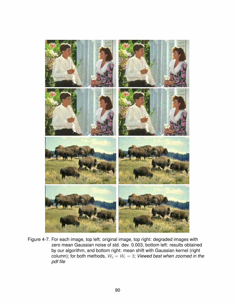
Figure 4-7. For each image, top left: original image, top right: degraded images withzero mean Gaussian noise of std. dev. 0.003, bottom left: results obtainedby our algorithm, and bottom right: mean shift with Gaussian kernel (rightcolumn); for both methods,Ws =Wr = 3; Viewed best when zoomed in thepdf file
90
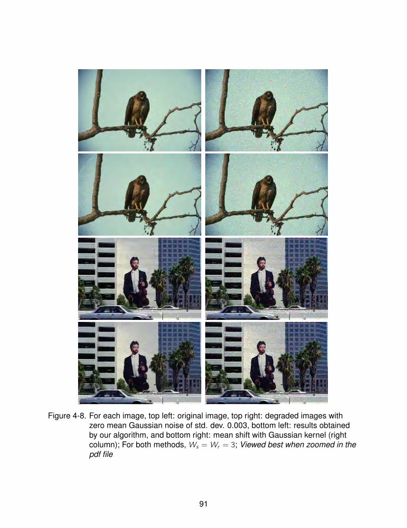
Figure 4-8. For each image, top left: original image, top right: degraded images withzero mean Gaussian noise of std. dev. 0.003, bottom left: results obtainedby our algorithm, and bottom right: mean shift with Gaussian kernel (rightcolumn); For both methods,Ws =Wr = 3; Viewed best when zoomed in thepdf file
91
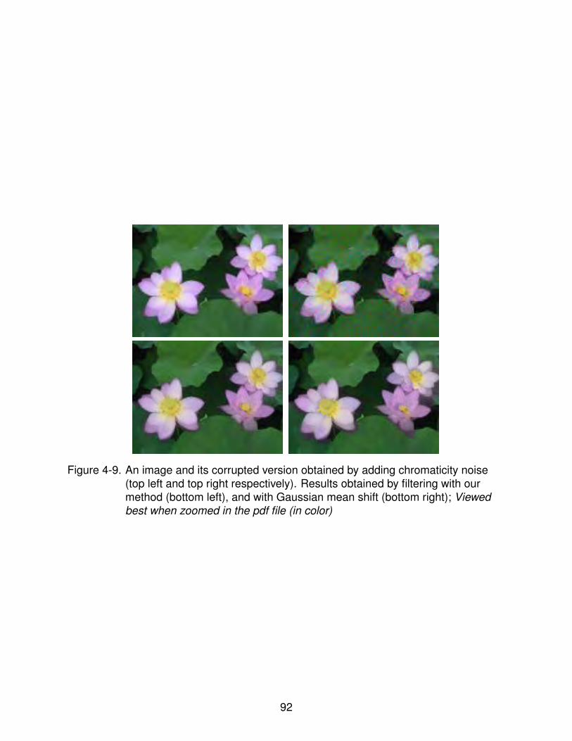
Figure 4-9. An image and its corrupted version obtained by adding chromaticity noise(top left and top right respectively). Results obtained by filtering with ourmethod (bottom left), and with Gaussian mean shift (bottom right); Viewedbest when zoomed in the pdf file (in color)
92
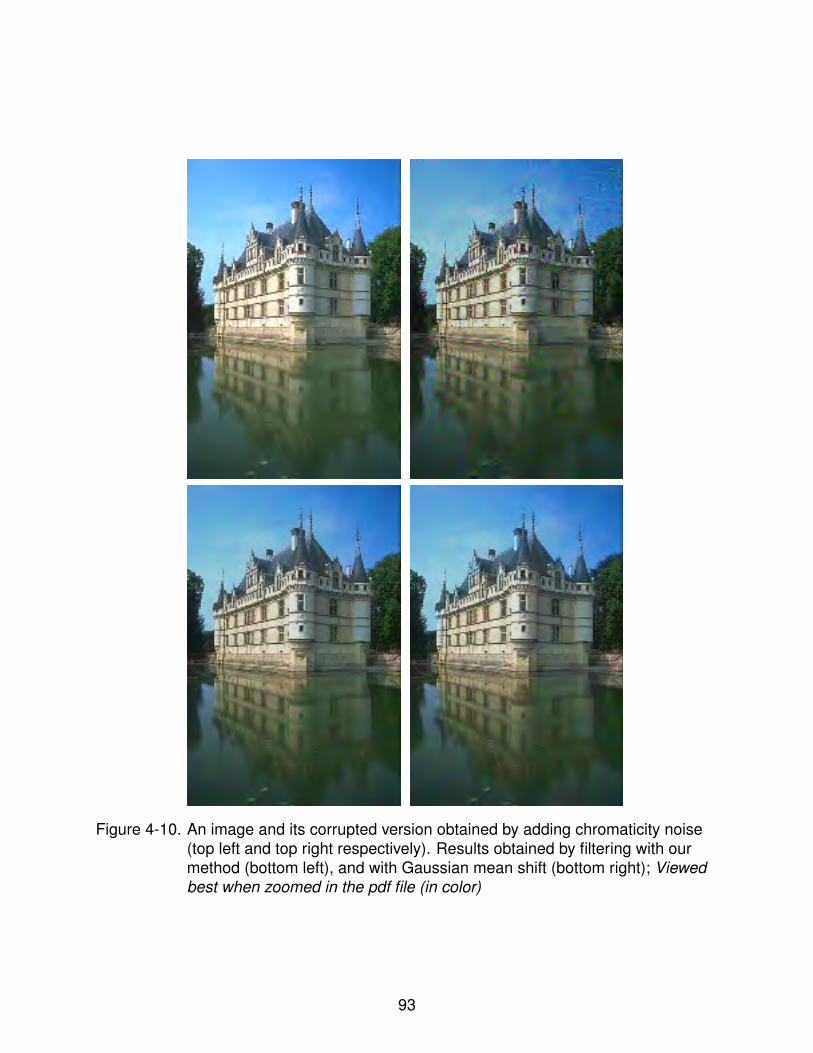
Figure 4-10. An image and its corrupted version obtained by adding chromaticity noise(top left and top right respectively). Results obtained by filtering with ourmethod (bottom left), and with Gaussian mean shift (bottom right); Viewedbest when zoomed in the pdf file (in color)
93
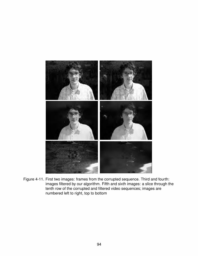
Figure 4-11. First two images: frames from the corrupted sequence. Third and fourth:images filtered by our algorithm. Fifth and sixth images: a slice through thetenth row of the corrupted and filtered video sequences; images arenumbered left to right, top to bottom
94
CHAPTER 5A RELATED PROBLEM: DIRECTIONAL STATISTICS IN EUCLIDEAN SPACE
5.1 Introduction
When the samples do not reside in Euclidean space, conventional density
estimation techniques such as mixtures of Gaussians or kernel density estimation
(KDE) using Gaussian kernels are not applied directly. For the special case when the
data reside on Sn, i.e. the sphere embedded in Rn, there exists extensive literature from
the field of directional statistics that is summarized in several exemplary books such as
[66]. Conventionally, for KDE or mixture model density estimation of unit vectors, the
Gaussian kernel has been replaced by von-Mises or von-Mises Fisher (voMF) kernels
for circular and spherical data respectively. These computational techniques have
been applied for solving numerous problems in computer vision, image processing,
medical imaging and computer graphics. Mixture modeling for directional data was
proposed originally by Kim et al. [67]. Banerjee et al. [68] also proposed a mixture
model for directional data and applied it for clustering problems. In medical imaging,
McGraw et al. [69] have modeled the displacement of water molecules in high angular
resolution diffusion images by means of a voMF mixture model. More recently, mixture
models of circular data have also been used for trajectory shape analysis in studying
object motion [70]. KDE of unit-vector data has been used in the context of smoothing
chromaticity vectors in color images [48]. Applications of such density estimators
in computer graphics include the work on approximation of the Torrance-Sparrow
Bidirectional Reflectance Functions (BRDF) as reported in [71], or the recent work in
[72] for approximating the distribution of surface normals. Eugeciouglu et al. [73] use a
kernel based on powers of cosines instead of a voMF in KDE, motivated by the superior
computational speed of the cosine estimator, and apply their technique for the analysis
of flow vectors in fluid mechanics.
95
The above techniques ignore the fact that the directional data are often obtained
as a transformation of the original measurements which are typically assumed to
reside in Euclidean space. Therefore the true probability density of the unit vector data
is related to that of the original data by means of a relationship dictated by random
variable transformations, a key concept in basic probability theory [74]. However,
a kernel density estimate or a mixture model estimate using (say) voMF kernels
ignores this very fundamental relationship. The technique proposed here exploits
exactly this relationship in the following way: (1) It performs density estimation in the
original space, and (2) It then transforms this density to the directional space using
random variable transformations. Thereby, it avoids the aforementioned inconsistency.
Secondly, conventional density estimation techniques for directional data also require
the solution of complicated nonlinear equations for key parameter updates such as
the covariance. This issue is completely circumvented by the presented technique.
A density estimator is built also for another directional quantity: hue in color images
(part of the HSI or hue-saturation-intensity color model), which is computed from a very
different transformation of the RGB color values obtained from a sensor (camera).
This chapter is organized as follows. Section 5.2 is a review on the choice of
kernel for density estimation for circular and spherical data. The drawbacks of these
approaches are enumerated and a new approach to density estimation for directional
data is introduced. This concept is extended for hue data in Section 5.3. A discussion is
presented in Section 5.4.
5.2 Theory
In this section, the theory of the new method is presented, starting with a review on
the choice of kernels for directional density estimation in contemporary vision literature.
5.2.1 Choice of Kernel
There exist a plethora of kernels used for estimating the density for unit vector
data, and the reasons for choosing one over the other require careful study. For KDE
96

of directional data, the voMF kernel is highly popular [69]. It has great computational
convenience because (1) it is symmetric, (2) it yields elegant closed-form formulae
for the Renyi entropy of a voMF mixture model, and for the distance between two
voMF distributions [69], and (3) the information-geometric properties of voMF mixtures
are simple [69]. Despite these algebraic properties, there are ambiguities [75] in the
oft-repeated [68] notion that the voMF is the ‘spherical analogue of the Gaussian’. The
voMF distribution does possess properties similar to a Gaussian such as those related
to maximum likelihood, and maximum differential entropy for fixed mean and variance,
besides symmetry. However, the voMF also differs from the Gaussian in the sense that
(1) the central limit theorem on the sphere does not involve the voMF but a uniform
distribution instead [75], (2) the voMF is not the solution to the isotropic heat equation
on the sphere [67] and (3) the convolution of two voMF distributions does not produce
exactly another voMF [66]. If we restrict ourselves to just the non-negative orthant of the
sphere (i.e. axial data), then the Bingham distribution also possesses many properties
similar to the Gaussian [75]. Another popular kernel for axial statistics is the Watson
distribution [76]. Some papers even consider a symmetrized version of the voMF kernel,
for instance [69]. However, the choice between Bingham, Watson and symmetrized
voMF kernels is unclear, and they will produce different density estimates for finite
sample sizes. Often, the motivation for choosing one over the other is computational
convenience, which is the chief reason behind the popularity of the voMF kernel.
5.2.2 Using Random Variable Transformation
The aforementioned density estimation techniques for directional data typically
assume that only the final unit vector data are available. However, very often in
computer vision applications, the original data are available as the output of a sensor.
These are then converted into unit vectors typically (though not always - see Section
5.3) by means of a projective transformation (unit normalization). The best instance
thereof is that color images are output by a camera usually in RGB format and
97
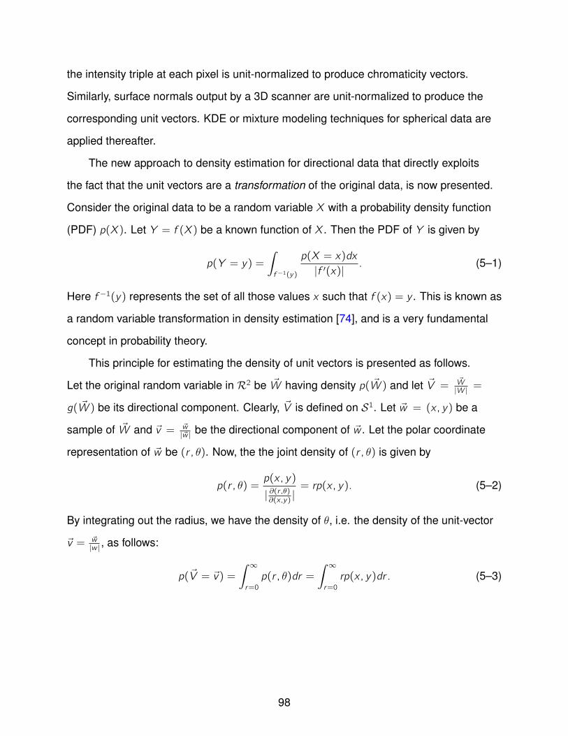
the intensity triple at each pixel is unit-normalized to produce chromaticity vectors.
Similarly, surface normals output by a 3D scanner are unit-normalized to produce the
corresponding unit vectors. KDE or mixture modeling techniques for spherical data are
applied thereafter.
The new approach to density estimation for directional data that directly exploits
the fact that the unit vectors are a transformation of the original data, is now presented.
Consider the original data to be a random variable X with a probability density function
(PDF) p(X ). Let Y = f (X ) be a known function of X . Then the PDF of Y is given by
p(Y = y) =
∫f −1(y)
p(X = x)dx
|f ′(x)|. (5–1)
Here f −1(y) represents the set of all those values x such that f (x) = y . This is known as
a random variable transformation in density estimation [74], and is a very fundamental
concept in probability theory.
This principle for estimating the density of unit vectors is presented as follows.
Let the original random variable in R2 be ~W having density p( ~W ) and let ~V = ~W|W | =
g( ~W ) be its directional component. Clearly, ~V is defined on S1. Let ~w = (x , y) be a
sample of ~W and ~v = ~w|~w | be the directional component of ~w . Let the polar coordinate
representation of ~w be (r , θ). Now, the the joint density of (r , θ) is given by
p(r , θ) =p(x , y)
| ∂(r ,θ)∂(x ,y)
|= rp(x , y). (5–2)
By integrating out the radius, we have the density of θ, i.e. the density of the unit-vector
~v = ~w|w | , as follows:
p(~V = ~v) =
∫ ∞
r=0
p(r , θ)dr =
∫ ∞
r=0
rp(x , y)dr . (5–3)
98
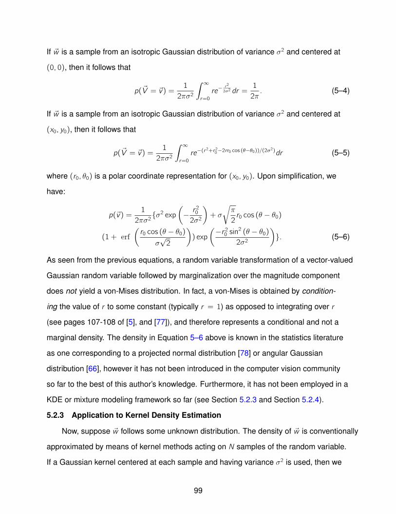
If ~w is a sample from an isotropic Gaussian distribution of variance σ2 and centered at
(0, 0), then it follows that
p(~V = ~v) =1
2πσ2
∫ ∞
r=0
re−r2
2σ2 dr =1
2π. (5–4)
If ~w is a sample from an isotropic Gaussian distribution of variance σ2 and centered at
(x0, y0), then it follows that
p(~V = ~v) =1
2πσ2
∫ ∞
r=0
re−(r2+r20−2rr0 cos (θ−θ0))/(2σ
2)dr (5–5)
where (r0, θ0) is a polar coordinate representation for (x0, y0). Upon simplification, we
have:
p(~v) =1
2πσ2σ2 exp
(− r
20
2σ2
)+ σ
√π
2r0 cos (θ − θ0)
(1 + erf
(r0 cos (θ − θ0)
σ√2
)) exp
(−r 20 sin2 (θ − θ0)
2σ2
). (5–6)
As seen from the previous equations, a random variable transformation of a vector-valued
Gaussian random variable followed by marginalization over the magnitude component
does not yield a von-Mises distribution. In fact, a von-Mises is obtained by condition-
ing the value of r to some constant (typically r = 1) as opposed to integrating over r
(see pages 107-108 of [5], and [77]), and therefore represents a conditional and not a
marginal density. The density in Equation 5–6 above is known in the statistics literature
as one corresponding to a projected normal distribution [78] or angular Gaussian
distribution [66], however it has not been introduced in the computer vision community
so far to the best of this author’s knowledge. Furthermore, it has not been employed in a
KDE or mixture modeling framework so far (see Section 5.2.3 and Section 5.2.4).
5.2.3 Application to Kernel Density Estimation
Now, suppose ~w follows some unknown distribution. The density of ~w is conventionally
approximated by means of kernel methods acting on N samples of the random variable.
If a Gaussian kernel centered at each sample and having variance σ2 is used, then we
99
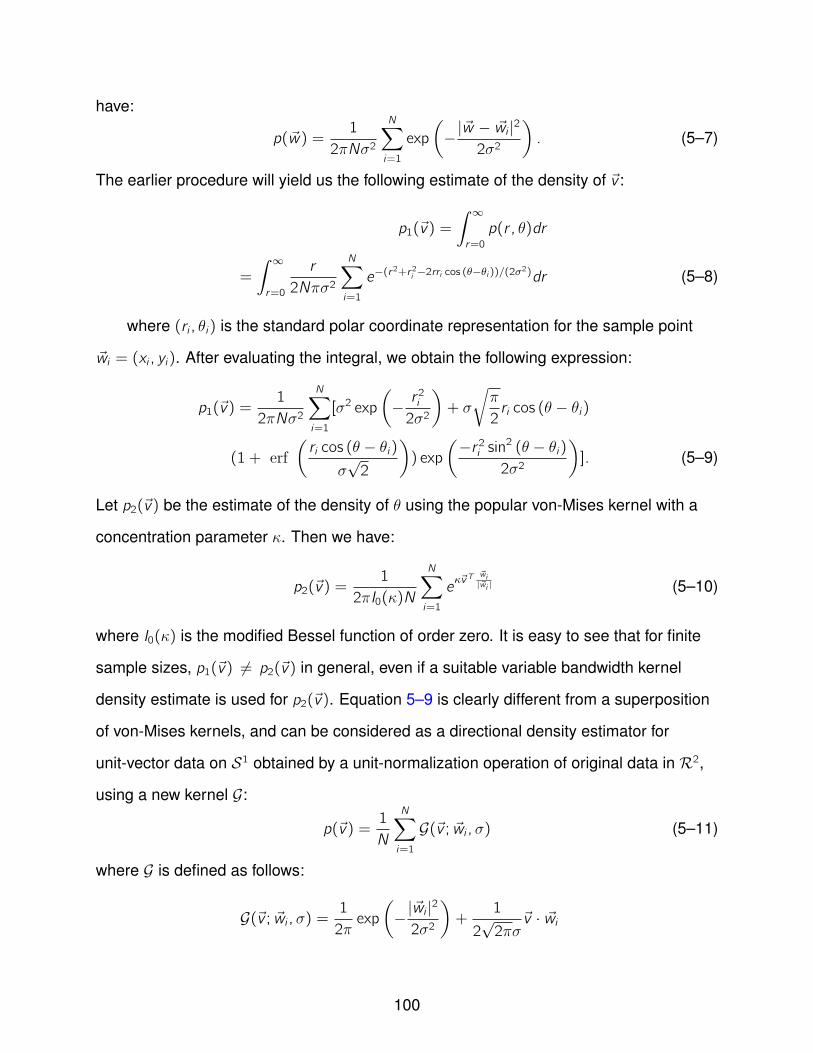
have:
p(~w) =1
2πNσ2
N∑i=1
exp
(−|~w − ~wi |2
2σ2
). (5–7)
The earlier procedure will yield us the following estimate of the density of ~v :
p1(~v) =
∫ ∞
r=0
p(r , θ)dr
=
∫ ∞
r=0
r
2Nπσ2
N∑i=1
e−(r2+r2i −2rri cos (θ−θi ))/(2σ
2)dr (5–8)
where (ri , θi) is the standard polar coordinate representation for the sample point
~wi = (xi , yi). After evaluating the integral, we obtain the following expression:
p1(~v) =1
2πNσ2
N∑i=1
[σ2 exp
(− r
2i
2σ2
)+ σ
√π
2ri cos (θ − θi)
(1 + erf
(ri cos (θ − θi)
σ√2
)) exp
(−r 2i sin
2 (θ − θi)
2σ2
)]. (5–9)
Let p2(~v) be the estimate of the density of θ using the popular von-Mises kernel with a
concentration parameter κ. Then we have:
p2(~v) =1
2πI0(κ)N
N∑i=1
eκ~vT
~wi|~wi | (5–10)
where I0(κ) is the modified Bessel function of order zero. It is easy to see that for finite
sample sizes, p1(~v) 6= p2(~v) in general, even if a suitable variable bandwidth kernel
density estimate is used for p2(~v). Equation 5–9 is clearly different from a superposition
of von-Mises kernels, and can be considered as a directional density estimator for
unit-vector data on S1 obtained by a unit-normalization operation of original data in R2,
using a new kernel G:
p(~v) =1
N
N∑i=1
G(~v ; ~wi ,σ) (5–11)
where G is defined as follows:
G(~v ; ~wi ,σ) =1
2πexp
(−|~wi |2
2σ2
)+
1
2√2πσ
~v · ~wi
100
(1 + erf
(~v · ~wiσ√2
))· exp
(−| ~wi |2 + (~v · ~wi)2
2σ2
). (5–12)
A similar PDF can be defined for unit vector data (denoted as ~v ) on S2, obtained by
projective transformation of data denoted as ~w = (x , y , z) residing in R3 belonging to
an isotropic Gaussian distribution centered at ~wi = (xi , yi , zi). This yields the following
expression:
p(~v) =
∫ ∞
r=0
r 2e−(x−xi )
2+(y−yi )2+(z−zi )
2
2σ2 dr . (5–13)
p(~v) =e
− ~|wi |2+(~v .~wi )
2
2σ2
2σ2(2π)1.5(√π
2[erf(
~v . ~wi
σ√2) + 1][(~v . ~wi)
2 + σ2] +σ
2~v . ~wie
− (~v .~wi )2
2σ2
). (5–14)
The key feature of the kernel density estimation approach in this section (and also the
pith of this chapter, in general) is that the model-fitting (selection of parameters such as
σ) can all be done in Euclidean space. The new kernels proposed in Equations 5–12
and 5–14 appear only in an emergent way out of the random variable transformation.
5.2.4 Mixture Models for Directional Data
Existing mixture modeling algorithms have difficulties associated with the choice
of the number of mixture components and local minima issues during model fitting.
Additionally, there are other practical difficulties involved in mixture modeling for the case
of directional data. Firstly, if von-Mises kernels [68] are used, the maximum-likelihood
estimate of the variance (or concentration parameter, often denoted as κ) is not
available in closed form and requires the solution to a non-linear equation involving
Bessel functions. In [68], the parameter κ is updated using various approximations for
the Bessel functions that are part of the normalization constant for voMF distributions,
followed by the addition of an empirically discovered bias that is a polynomial function of
the estimated mean vectors. The difficulties faced by a mixture of voMF distributions in
modeling data that are spread out anisotropically are mitigated by the use of a mixture
101
of Watson kernels as claimed in [76]. Nonetheless, iterative numerical procedures to
estimate κ are still required, and the case where a full covariance is to be obtained, will
be even more complicated. Moreover the method in [76] also requires solving non-linear
equations for the update of the centers of the individual components over and above
the κ values. Over and above this, the update of the mean vectors in both [68] and [76]
involves vector addition followed by unit normalization, which is unstable if antipodal
vectors are involved as the norm of the resultant vector will be very small.
The approach based on the theory presented in the previous subsections
overcomes these difficulties by following a two-step procedure: (1) a mixture-model fit in
the original Euclidean space given a set of N samples, followed by (2) a transformation
of random variables. If a Gaussian mixture model is fit to the original data samples,
using M components, with priors pk, centers (µxk ,µyk) = (rk cos θk , rk sin θk) and
variances σk, then a random variable transformation results in the following form of
directional mixture model:
p(~v) =
∫ ∞
r=0
r
2πσ2
M∑k=1
pke−(x−µxk )
2+(y−µyk )2
2σ2k dr ,
p(~v) =
M∑k=1
pkG(~v ; ~µk ,σk), (5–15)
where G was defined in Equation 5–12. Since the entire mixture-modeling procedure is
performed in the original space, the aforementioned difficulties in estimating the mean
and concentration parameters are automatically avoided.
If we continue to follow this line of reasoning, we can now achieve a fresh
perspective on mixtures of voMF distributions as well. As mentioned previously and as
clearly documented in [5], the voMF distribution is obtained from a Gaussian distribution
by conditioning the magnitude of the random variable to be some constant. If we fit a
Gaussian mixture model to the original data and expressed it in polar coordinates, we
102
are left with the following expression:
p(r , θ) =M∑k=1
pk2πσ2k
e− (r cos θ−rk cos θk )
2+(r sin θ−rk sin θk )2
2σ2k . (5–16)
By conditioning on r = 1, we have:
p(θ|r = 1) =M∑k=1
pk2πI0(
rkσ2k)erk cos (θ−θk )
σ2k . (5–17)
This procedure basically suggests again that the entire mixture modeling algorithm
can be executed in Euclidean space, and that a mixture of voMF distributions can be
obtained by conditioning the magnitude of the random variable to be 1 (or some other
constant)1 . The polar coordinates transformations yield a formula for the concentration
parameter κk of the k th component, given as κk = rkσ2k
. This procedure therefore suggests
us a viable alternative to fitting a mixture of voMF distributions when the original data are
available (and not just the unit-vector data). Similar expressions can be derived for the
case of data on S2 derived from R3 as well.
5.2.5 Properties of the Projected Normal Estimator
The projected normal distribution is symmetric and unimodal just like the von-Mises
distribution. Figure 5-1 shows the projected normal distribution corresponding to an
original Gaussian distribution centered at ~µ0 = (1, 0) having a variance of σ0 = 10,
and a von-Mises distribution centered at (1, 0) with κ0 =|~µ0|σ20= 0.01. Similarly, plots
of the projected normal distribution on S2 for an original Gaussian distribution with
~µ0 = (1, 0, 0) and variance 10, and a voMF distribution with mean ~µ0 = (1, 0, 0)
and concentration κ0 =|~µ0|σ2
are shown in Figure 5-2. As indicated by the plots, both
distributions have a distinct peak at θ ≈ 54,φ ≈ 45 as expected.
1 Note that the voMF distribution or a mixture of voMF distributions are conditional andnot marginal distributions.
103
From Equations 5–9, 5–12 and 5–14, it can be seen that the density estimator does
not require the conversion of the original samples to unit vectors, but operates entirely in
the original space.
5.3 Estimation of the Probability Density of Hue
Directional data are usually obtained by the process of unit-normalization of
the original vector data measured by a sensor. However, this isn’t always the case.
For instance, color sensors typically output values in the RGB color format. These
values are then converted to other color systems such as HSI using transformations
of a different kind, presented below. The HSI color model is based on the notion of
separating a color into three quantities - the hue H (which is the basic color such as red
or green), the saturation S (which indicates the amount of white present in a color) and
the value I (which indicates the amount of shading or black). The component hue (H) is
an angular quantity. The rules for conversion between the RGB and HSI color models
are as follows [48]:
H = cos−1
(0.5(2R − G − B)√
(R − G)2 + (R − B)(G − B)
)S = 1− 3
R + G + Bmin(R,G ,B)
I =1
3(R + G + B). (5–18)
The inverse transformation from HSI to RGB, for hue values 0 < H ≤ 2π3
, is:
B = I (1− S)
R = I (1 +S cosH
cos(π3− H)
)
G = 3I − (R + B). (5–19)
For hue values 2π3< H ≤ 4π
3, the formulae are given by:
H = H − 2π3
R = I (1− S)
104
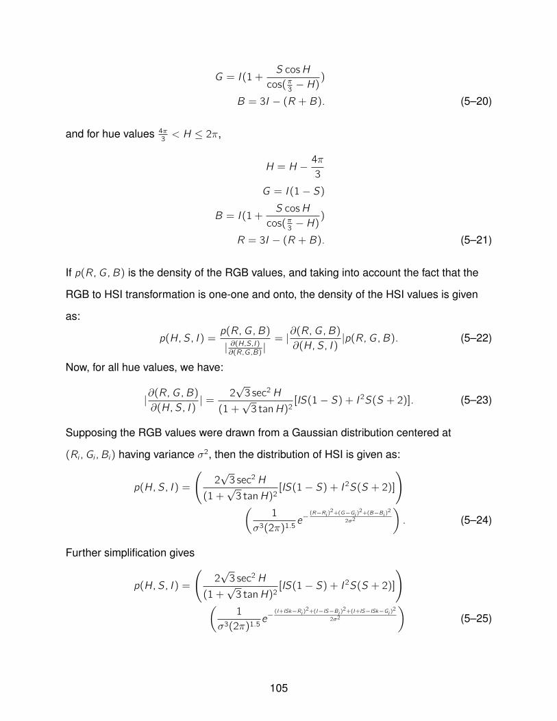
G = I (1 +S cosH
cos(π3− H)
)
B = 3I − (R + B). (5–20)
and for hue values 4π3< H ≤ 2π,
H = H − 4π3
G = I (1− S)
B = I (1 +S cosH
cos(π3− H)
)
R = 3I − (R + B). (5–21)
If p(R,G ,B) is the density of the RGB values, and taking into account the fact that the
RGB to HSI transformation is one-one and onto, the density of the HSI values is given
as:
p(H,S , I ) =p(R,G ,B)
| ∂(H,S,I )∂(R,G ,B)
|= |∂(R,G ,B)
∂(H,S , I )|p(R,G ,B). (5–22)
Now, for all hue values, we have:
|∂(R,G ,B)∂(H,S , I )
| = 2√3 sec2H
(1 +√3 tanH)2
[IS(1− S) + I 2S(S + 2)]. (5–23)
Supposing the RGB values were drawn from a Gaussian distribution centered at
(Ri ,Gi ,Bi) having variance σ2, then the distribution of HSI is given as:
p(H,S , I ) =
(2√3 sec2H
(1 +√3 tanH)2
[IS(1− S) + I 2S(S + 2)]
)(
1
σ3(2π)1.5e−
(R−Ri )2+(G−Gi )
2+(B−Bi )2
2σ2
). (5–24)
Further simplification gives
p(H,S , I ) =
(2√3 sec2H
(1 +√3 tanH)2
[IS(1− S) + I 2S(S + 2)]
)(
1
σ3(2π)1.5e−
(I+ISk−Ri )2+(I−IS−Bi )
2+(I+IS−ISk−Gi )2
2σ2
)(5–25)
105
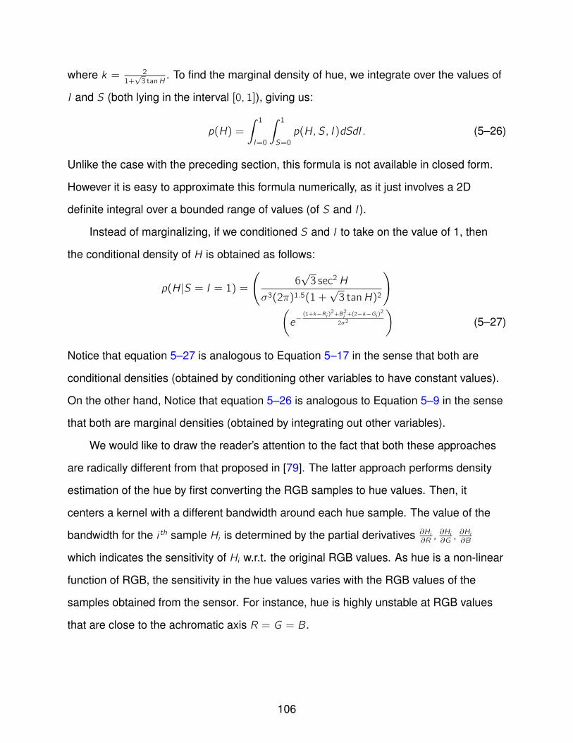
where k = 2
1+√3 tanH
. To find the marginal density of hue, we integrate over the values of
I and S (both lying in the interval [0, 1]), giving us:
p(H) =
∫ 1I=0
∫ 1S=0
p(H,S , I )dSdI . (5–26)
Unlike the case with the preceding section, this formula is not available in closed form.
However it is easy to approximate this formula numerically, as it just involves a 2D
definite integral over a bounded range of values (of S and I ).
Instead of marginalizing, if we conditioned S and I to take on the value of 1, then
the conditional density of H is obtained as follows:
p(H|S = I = 1) =
(6√3 sec2H
σ3(2π)1.5(1 +√3 tanH)2
)(e−
(1+k−Ri )2+B2i +(2−k−Gi )
2
2σ2
)(5–27)
Notice that equation 5–27 is analogous to Equation 5–17 in the sense that both are
conditional densities (obtained by conditioning other variables to have constant values).
On the other hand, Notice that equation 5–26 is analogous to Equation 5–9 in the sense
that both are marginal densities (obtained by integrating out other variables).
We would like to draw the reader’s attention to the fact that both these approaches
are radically different from that proposed in [79]. The latter approach performs density
estimation of the hue by first converting the RGB samples to hue values. Then, it
centers a kernel with a different bandwidth around each hue sample. The value of the
bandwidth for the i th sample Hi is determined by the partial derivatives ∂Hi∂R, ∂Hi∂G, ∂Hi∂B
which indicates the sensitivity of Hi w.r.t. the original RGB values. As hue is a non-linear
function of RGB, the sensitivity in the hue values varies with the RGB values of the
samples obtained from the sensor. For instance, hue is highly unstable at RGB values
that are close to the achromatic axis R = G = B.
106
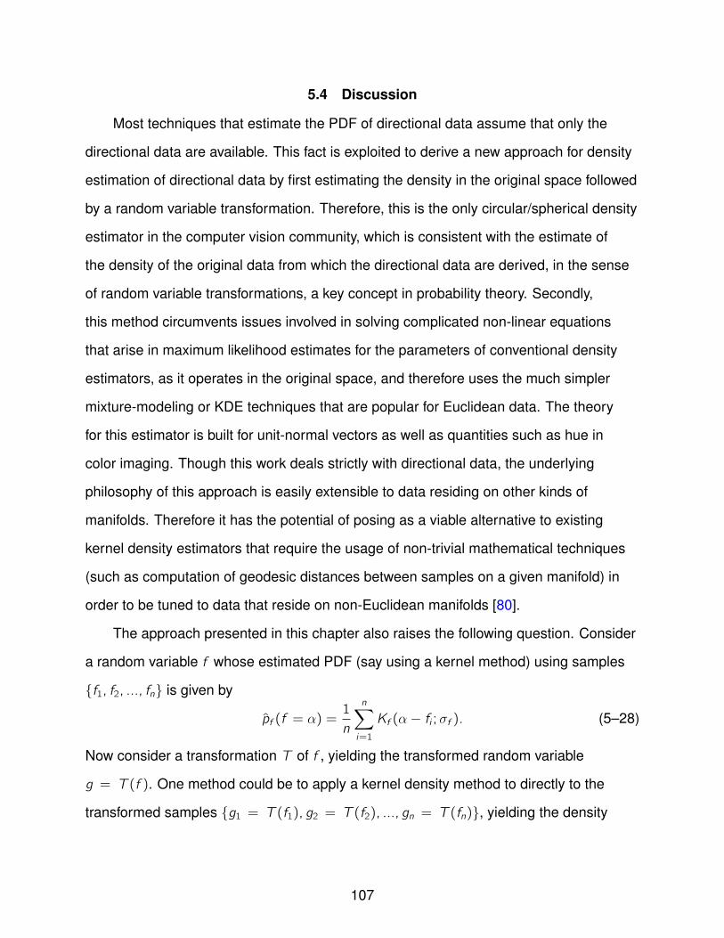
5.4 Discussion
Most techniques that estimate the PDF of directional data assume that only the
directional data are available. This fact is exploited to derive a new approach for density
estimation of directional data by first estimating the density in the original space followed
by a random variable transformation. Therefore, this is the only circular/spherical density
estimator in the computer vision community, which is consistent with the estimate of
the density of the original data from which the directional data are derived, in the sense
of random variable transformations, a key concept in probability theory. Secondly,
this method circumvents issues involved in solving complicated non-linear equations
that arise in maximum likelihood estimates for the parameters of conventional density
estimators, as it operates in the original space, and therefore uses the much simpler
mixture-modeling or KDE techniques that are popular for Euclidean data. The theory
for this estimator is built for unit-normal vectors as well as quantities such as hue in
color imaging. Though this work deals strictly with directional data, the underlying
philosophy of this approach is easily extensible to data residing on other kinds of
manifolds. Therefore it has the potential of posing as a viable alternative to existing
kernel density estimators that require the usage of non-trivial mathematical techniques
(such as computation of geodesic distances between samples on a given manifold) in
order to be tuned to data that reside on non-Euclidean manifolds [80].
The approach presented in this chapter also raises the following question. Consider
a random variable f whose estimated PDF (say using a kernel method) using samples
f1, f2, ..., fn is given by
pf (f = α) =1
n
n∑i=1
Kf (α− fi ;σf ). (5–28)
Now consider a transformation T of f , yielding the transformed random variable
g = T (f ). One method could be to apply a kernel density method to directly to the
transformed samples g1 = T (f1), g2 = T (f2), ..., gn = T (fn), yielding the density
107
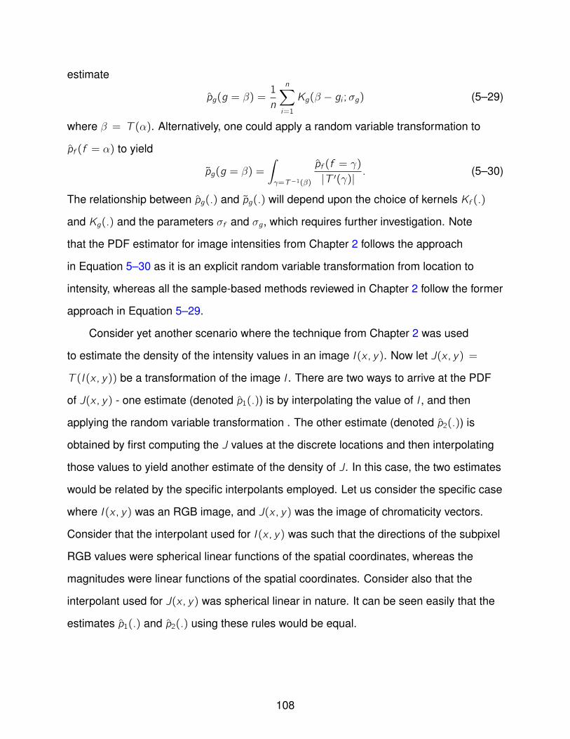
estimate
pg(g = β) =1
n
n∑i=1
Kg(β − gi ;σg) (5–29)
where β = T (α). Alternatively, one could apply a random variable transformation to
pf (f = α) to yield
pg(g = β) =
∫γ=T−1(β)
pf (f = γ)
|T ′(γ)|. (5–30)
The relationship between pg(.) and pg(.) will depend upon the choice of kernels Kf (.)
and Kg(.) and the parameters σf and σg, which requires further investigation. Note
that the PDF estimator for image intensities from Chapter 2 follows the approach
in Equation 5–30 as it is an explicit random variable transformation from location to
intensity, whereas all the sample-based methods reviewed in Chapter 2 follow the former
approach in Equation 5–29.
Consider yet another scenario where the technique from Chapter 2 was used
to estimate the density of the intensity values in an image I (x , y). Now let J(x , y) =
T (I (x , y)) be a transformation of the image I . There are two ways to arrive at the PDF
of J(x , y) - one estimate (denoted p1(.)) is by interpolating the value of I , and then
applying the random variable transformation . The other estimate (denoted p2(.)) is
obtained by first computing the J values at the discrete locations and then interpolating
those values to yield another estimate of the density of J. In this case, the two estimates
would be related by the specific interpolants employed. Let us consider the specific case
where I (x , y) was an RGB image, and J(x , y) was the image of chromaticity vectors.
Consider that the interpolant used for I (x , y) was such that the directions of the subpixel
RGB values were spherical linear functions of the spatial coordinates, whereas the
magnitudes were linear functions of the spatial coordinates. Consider also that the
interpolant used for J(x , y) was spherical linear in nature. It can be seen easily that the
estimates p1(.) and p2(.) using these rules would be equal.
108
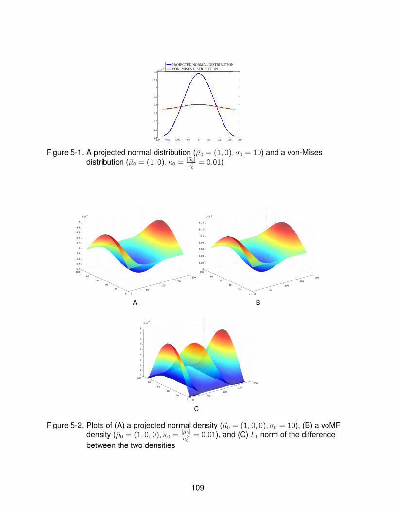
−200 −150 −100 −50 0 50 100 150 2002.4
2.5
2.6
2.7
2.8
2.9
3
3.1
3.2x 10
−4
PROJECTED NORMAL DISTRIBUTIONVON−MISES DISTRIBUTION
Figure 5-1. A projected normal distribution (~µ0 = (1, 0),σ0 = 10) and a von-Misesdistribution (~µ0 = (1, 0),κ0 =
|~µ0|σ20= 0.01)
0
50
100
150
200
0
20
40
60
80
1005.2
5.4
5.6
5.8
6
6.2
6.4
6.6
6.8
7
x 10−5
A
0
50
100
150
200
0
20
40
60
80
1006
6.02
6.04
6.06
6.08
6.1
6.12
6.14
x 10−5
B
0
50
100
150
200
0
20
40
60
80
1000
1
2
3
4
5
6
7
8
9
x 10−6
C
Figure 5-2. Plots of (A) a projected normal density (~µ0 = (1, 0, 0),σ0 = 10), (B) a voMFdensity (~µ0 = (1, 0, 0),κ0 =
|~µ0|σ20= 0.01), and (C) L1 norm of the difference
between the two densities
109
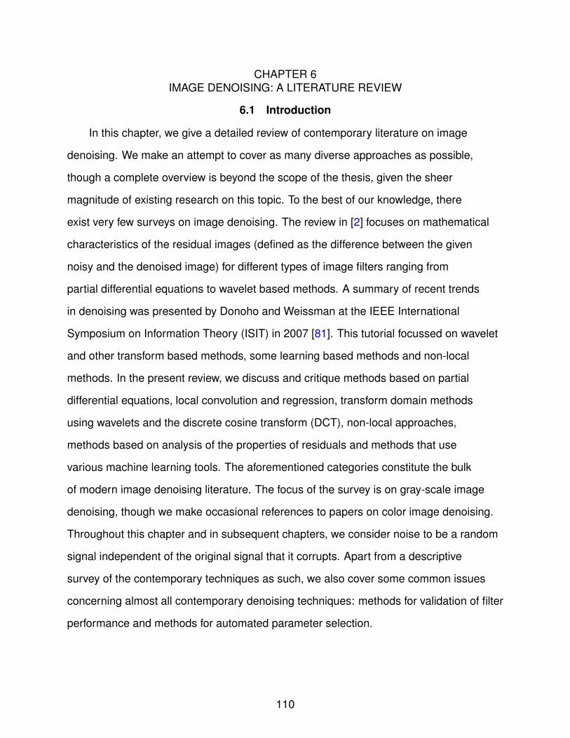
CHAPTER 6IMAGE DENOISING: A LITERATURE REVIEW
6.1 Introduction
In this chapter, we give a detailed review of contemporary literature on image
denoising. We make an attempt to cover as many diverse approaches as possible,
though a complete overview is beyond the scope of the thesis, given the sheer
magnitude of existing research on this topic. To the best of our knowledge, there
exist very few surveys on image denoising. The review in [2] focuses on mathematical
characteristics of the residual images (defined as the difference between the given
noisy and the denoised image) for different types of image filters ranging from
partial differential equations to wavelet based methods. A summary of recent trends
in denoising was presented by Donoho and Weissman at the IEEE International
Symposium on Information Theory (ISIT) in 2007 [81]. This tutorial focussed on wavelet
and other transform based methods, some learning based methods and non-local
methods. In the present review, we discuss and critique methods based on partial
differential equations, local convolution and regression, transform domain methods
using wavelets and the discrete cosine transform (DCT), non-local approaches,
methods based on analysis of the properties of residuals and methods that use
various machine learning tools. The aforementioned categories constitute the bulk
of modern image denoising literature. The focus of the survey is on gray-scale image
denoising, though we make occasional references to papers on color image denoising.
Throughout this chapter and in subsequent chapters, we consider noise to be a random
signal independent of the original signal that it corrupts. Apart from a descriptive
survey of the contemporary techniques as such, we also cover some common issues
concerning almost all contemporary denoising techniques: methods for validation of filter
performance and methods for automated parameter selection.
110
6.2 Partial Differential Equations
The isotropic heat equation was used for image smoothing in [82]. It is known
that executing this partial differential equation (PDE) on the image is equivalent to
convolution with a Gaussian kernel, where the kernel parameter (often denoted
by σ) is related to the time step and number of iterations of the PDE. However,
isotropic smoothing blurs away significant image features such as edges along with
the noise, and hence is not used in contemporary denoising algorithms. Instead, in most
contemporary diffusion methods, the diffusion process is directed by edge information
in the form of a diffusivity function which prevents blurring across edges and allows
diffusion along them [44]. The chosen diffusivity function is actually a monotonically
decreasing function of the gradient magnitude. The equation for the PDE can be written
as follows∂I
∂t= div(g(|∇I |)∇I ) (6–1)
where I : Ω → R is a gray-scale image defined on domain Ω and g(|∇I |) is a diffusivity
function typically defined as
g(|∇I |;λ) = 1
1 + |∇I |2/λ2. (6–2)
Several different diffusivity functions have been proposed, for instance those by Perona
and Malik [44], Weickert [83] and Black et al. [84]. A regularized version of the above
equation has been proposed in [85]. Connections between robust statistics and
anisotropic diffusion (which show up in the choice of diffusivity function) have been
established in [84].
Some PDEs are obtained from the Euler-Lagrange equations corresponding to
energy functionals. One example is the image total variation defined as
E(I ) =
∫Ω
|∇I (x , y)|dxdy (6–3)
111
giving rise to the PDE∂I
∂t= div(
∇I|∇I |). (6–4)
It should be noted that the aforementioned techniques are based on the assumption
that natural images are piecewise constant, which is not necessarily a valid assumption.
They also require the choice of the parameter λ in the diffusivity. This parameter need
not be constant throughout the image. The number of iterations for which these PDEs
are executed is an important parameter critical for good performance. In the limit of
infinite iterations, constant or piecewise-constant images are produced. Some authors
remedy the stopping time selection issue by introducing a prior model in the energy
formulation, for example the following modification of the total variation model, starting
with an initial image I0
E(I ) =
∫Ω
|∇I (x , y)|dxdy + µ∫Ω
(I (x , y)− I0(x , y))2dxdy (6–5)
where µ is a parameter that trades data fidelity with regularity. The implicit assumption
in the term (I (x , y) − I0(x , y))2 is a Gaussian noise model. Assuming that the image
has been corrupted with zero mean Gaussian noise of known variance σ2n, a constrained
version of the objective function has been proposed in [86]:
minIE(I ) =
∫Ω
|∇I (x , y)|dxdy (6–6)
subject to ∫Ω
(I − I0)2dxdy = σ2n (6–7)∫Ω
I (x , y)dxdy =
∫Ω
I0(x , y)dxdy . (6–8)
For different noise models, such as Poisson or impulse noise, different priors can be
used [87]. A highly comprehensive review of several such PDE-based approaches can
be found in exemplary books such as [83] and [53], to name a few. Recently, some
authors have also introduced the concept of diffusion with complex numbers, which
112
brings about denoising in conjunction with edge enhancement [88], [89]. The latter
technique performs the complex diffusion by treating the image I : Ω → R as a graph of
the form (x , y , I (x , y)), a framework for diffusion developed in [58].
Some researchers have developed PDEs based on a piecewise linear assumption
on natural images, examples being [90] and [91]. These turn out to be fourth order
PDEs and their energy functions penalize deviation in the intensity gradient as opposed
to deviation in intensity, and preserve fine shading better. However in some cases such
as [90], speckle artifacts have been observed which need to be retroactively remedied
using median filters [90]. Another class of approaches consists of independently filtering
the gradients in the x and y directions, and then using some prior assumption on the
image geometry to reconstruct the image intensity from the smoothed gradient values
[92].
6.3 Spatially Varying Convolution and Regression
A rich class of techniques for image filtering involve the so-called spatially varying
convolutions. In these methods, an image is convolved with a pointwise varying mask
which is derived from the local geometry extracted from the signal. A closely related
idea is the modeling of the local geometry of an image (signal) by means of a low-order
polynomial function. The signal is approximated locally by a pointwise-varying weighted
polynomial fit. The coefficients of the polynomial are computed by a least-squares
regression, and these are then used to compute the value of the (filtered) signal at
a central point. For instance, the signal could be modeled as follows, restricted to a
neighborhood Ω around a point x0:
I (x) = a0 +
m∑i=1
ai(x − x0)i (6–9)
where ai (0 ≤ i ≤ m) are coefficients of the polynomial. These coefficients are
obtained by least squares fitting, and the filtered signal value is given by I (x0) = a0.
This procedure is not guaranteed to preserve edges as it allows even disparate intensity
113
values to affect the polynomial fit. Instead in practice, the signal is modeled as follows:
I (x) = a0 +
m∑i=1
aiw(x − x0, I (x)− I (x0); hs , hv)(x − x0)i . (6–10)
Here w(x − x0, I (x) − I (x0); hs , hv) is a weighting scheme which is basically a
non-increasing function of the difference between spatial locations, i.e. x − x0, and
the difference between the signal values at those locations, i.e. I (x) − I (x0). The
function w is parameterized by hs and hv which act as spatial and intensity smoothing
parameters respectively. The fitting procedure is now, of course, a weighted least
squares regression. These ideas trace back to the Savitzky-Golay filter [93], [94] and
are the subject of beautiful books such as [95]. Two-dimensional versions of these ideas
have been recently used in modified forms for image filtering applications in [65] and
[55]. In [65], the parameter hs is replaced by a matrix, which is selected in a manner
dictated by local image edge geometry and no penalty is applied on intensity deviation.
On the other hand, in the latter case [55], the weights for regression are affected solely
by intensity difference. The popular bilateral filtering technique [49], [96] is again based
on a weighted linear combination of intensities, with weights driven by both location and
intensity differences. In fact, the kernel regression approach in [65] has been framed as
a higher-order generalization of the bilateral filter. If the polynomial order is restricted to
one and the weights are applied only on intensity differences, one gets the so-called the
kernel density based filter [48], also called as the anisotropic neighborhood filter [55].
A version where the weights are obtained from intensity gradient magnitudes has been
presented in [47] and is called as the adaptive filter. An extension to the anisotropic
neighborhood filter using interpolation between noisy image intensity values (and the
induced isocontour map) has been recently presented by us in [11] and in Chapter
4. In all these techniques, a crucial parameter is the size and also the shape of the
neighborhood for local signal modeling. An important contribution toward solving this
114
problem is a data-driven approach presented in [97], which derives a multi-directional
star-shaped neighborhood (of largest possible size) around each image pixel.
The mean-shift procedure, a clustering technique proposed in [98], and applied to
filtering (and segmentation) in [51], can be considered as a generalization of bilateral
filtering, where the window for local signal modeling is allowed to grow dynamically.
This growth is directed by an ascent on a local joint density function of spatial as well
as intensity values. It should be noted that both bilateral filtering and mean shift are
related to the Beltrami flow PDE developed in [58]. These relationships have been
explored in [99]. The connections between nonlinear diffusion PDEs over small periods
of time and spatially varying convolutions have been shown in [100]. In [45], the authors
present so-called trace-based PDEs for smoothing of color images and prove that the
corresponding diffusion is exactly equivalent to convolutions with oriented Gaussians,
where the orientation is dictated by local image geometry or edge direction.
Thus, spatially varying convolutions for filtering have a rich history. The most recent
contribution in this area is the one presented in [64] and [101]. This framework is based
upon the Jian-Vemuri continuous mixture model from the field of diffusion-weighted
magnetic resonance imaging (DW-MRI) [102]. In [64], complicated local image
geometries such as edges as well as X, Y or T junctions are modeled using a Gabor
filter bank at different orientations. The collection of Gabor-filter responses is expressed
as a discrete mixture of a continuous mixture of Gaussians (with Wishart mixing
densities) or a discrete mixture of a continuous mixture of Watson distributions (with
Bingham mixing densities) to respectively yield two different types of kernels for local
geometry-preserving convolutions. The number of components of the discrete mixture
is given by an appropriate sampling of the 2D orientation space and the weights of the
discrete mixture are solved by local regularized least squares fitting. The novelty of this
technique is (1) the automatic setting of weights for geometry-preserving smoothing,
and (2) the ability to preserve features such as image corners and junctions (which are
115
ignored by the other convolution-based methods mentioned before). While techniques
such as curvature-preserving PDEs [103] attempt preservation of such geometries,
their behavior at X, Y or T junctions (where curvature is not defined) may need further
exploration.
The mean shift procedure or other local convolution filters can also be applied to
the image gradients to better facilitate the preservation of shading. An extensive survey
of various applications with different types of filtering operations on image gradients,
followed by image reconstruction using a projection onto the nearest integrable surface
[104] or by solving the Poisson equation, has been presented in [105] in a short course
at the International Conference on Computer Vision, 2007, and in papers such as [106].
6.4 Transform-Domain Denoising
Transform-domain denoising approaches typically work at the level of small image
patches. In these approaches, the image patch is projected onto a chosen orthonormal
basis (such as a wavelet basis or the DCT basis) to yield a set of coefficients. It is
well-known that the coefficients in the transform domain are highly compressible in the
sense that the vast majority of these coefficients are very close to zero. In the literature,
this property is referred to as ‘sparsity’, though in a strict sense, sparsity would require
most coefficients to be equal to zero. In the rest of the thesis, we shall stick to this
usage of the word ‘sparsity’ even though we imply compressibility. It is known that the
coefficients in the wavelet or DCT transform domain are decorrelated from one another
[107]. It should be noted that the smaller coefficients usually correspond to the higher
frequency components of the signal which are often dominated by noise. To perform
denoising, the smaller coefficients are modified (typically, those coefficients whose
magnitude is below some λ are set to zero, in a process termed ‘hard thresholding’), and
the patch is reconstructed by inversion of the transform. This procedure is repeated for
every patch. If the patches are chosen to be non-overlapping, one can observe seam
artifacts at the patch boundaries. Furthermore, the thresholding of the coefficients is
116
also known to produce ringing artifacts around image edges or salient features. Artifacts
of both types can be remedied by performing the aforementioned three steps in a sliding
window fashion from pixel to pixel. This yields an overcomplete transform as each
pixel now acquires multiple hypotheses from overlapping patches. These hypotheses
are aggregated (typically by simple averaging) together to yield a final estimate. This
process of averaging of multiple hypotheses has been reported to consistently yield
superior results [108], [109], and is termed ‘translation invariant denoising’, or ‘cycle
spinning’ [108].
The performance of transform-based techniques is affected by the following
parameters: the choice of basis, the choice of a thresholding mechanism, a method
for aggregation of overlapping estimates and the patch size. We discuss these points
below.
6.4.1 Choice of Basis
Somewhat surprisingly, it has been observed that the sliding window DCT
outperforms most wavelet bases [109]. However, given a library of orthonormal bases,
the choice of the best one (from the point of view of denoising) from amongst these, is
largely an open problem in signal processing. In many existing approaches, the image
patch (of size n1 × n2) is represented as a matrix and the bases for representation are
obtained from the outer product of the bases that represent the rows with the bases
that represent the columns [109], [108]. This is called as a separable representation. In
other cases, the image patch is represented as a 1D vector of size n1n2 using a basis
of size n1n2 × n1n2. In the separable case, it has been observed that the transform may
be biased towards images whose salient features are aligned with the Cartesian axes.
If the local image geometry deviates from these axes, the transform may not be able
to represent them compactly enough. This has been remedied by using non-separable
bases such as the steerable wavelet [110], or the curvelet transform [111], which are
designed by taking image geometry into account.
117

6.4.2 Choice of Thresholding Scheme and Parameters
The most common thresholding method is hard thresholding, given as follows:
T (c ;λ) =
c if |c | ≥ λ
0 if |c | < λ.(6–11)
Another popular method, known as soft thresholding, not only nullifies coefficients
smaller than the threshold but also reduces the value of coefficients that are larger than
the threshold. Mathematically, soft thresholding is expressed as follows:
T (c ;λ) =
c − λ if |c | > λ, c > 0
c + λ if |c | > λ, c < 0
0 if |c | < λ
(6–12)
There exist several other thresholding schemes (or rather, schemes for modification of
transform coefficients). These methods can be interpreted as the result of minimizing
different types of risk functions. For example, the hard thresholding scheme (sometimes
termed as the best subset selection problem) is the result of minimizing the hard
threshold penalty, soft thresholding has an interpretation in terms of minimizing
the L1 penalty, whereas minimization of the smoothly clipped absolute deviation
(SCAD) leads to a thresholding scheme that lies intermediate between hard and soft
thresholding (see Figures 1 and 2 and Section (2.1) of [112]). Almost all these methods
of thresholding lead to monotonic functions of the coefficient magnitude. Despite the
several sophisticated thresholding functions available, the best denoising results that
have been reported using wavelet transforms are the ones with hard thresholding,
with a translation invariant approach [62]. The choice of the parameter λ has been
studied in detail in the community. For instance, in [113], the authors prove that under
a hard thresholding scheme, the choice λ = σn√2 logN is optimal from a statistical
risk standpoint, under zero mean Gaussian noise of standard deviation σn, where
N is the size (i.e. number of pixels) of the image/image patch (see Theorem (4) and
118
Equation (31) of [113]). In the experiments to be presented in Chapter 7, we have
observed empirically that the threshold λ = 3σ produces excellent denoising results for a
Gaussian noise model with 8×8 patches, which approximately tallies with the result from
[113]. This is in tune with an empirically observed fact that the coefficients of a Gaussian
random matrix of standard deviation σ when projected on an orthonormal basis are less
than 3σ with a very high probability.
6.4.3 Method for Aggregation of Overlapping Estimates
The most common approach for aggregation is a simple averaging of (or a median
operation on) all the hypotheses generated for the pixel.
6.4.4 Choice of Patch Size
The patch size choice presents the classical bias-variance tradeoff. Very small
patches allow preservation of finer details of the image but may overfit (undersmooth),
whereas larger patch sizes perform better in smoothing larger homogeneous regions
but may oversmooth some subtle details. Very little work exists on optimal patch
size selection. In fact, the patch size need not be constant throughout the image
and can vary as per local geometry. Some papers such as [114] propose the use of
multi-scale approaches by combining estimates at different scales. However the optimal
combination of such estimates is still a problem, much like that of optimal aggregation of
overlapping estimates. We present a correlation-coefficient criterion for the automated
selection of a single global patch size in Chapter 7.
A common criticism of transform-domain thresholding techniques (especially hard
thresholding) is their inability to distinguish high frequency information from noise. Some
authors try to remedy this by observing that there exist dependencies that arise in a
transform coefficients at the same spatial location but at different scales [115], or at
adjacent spatial locations [116]. These dependencies are exploited by using multivariate
thresholding methods. For instance in [115], bivariate shrinkage rules are developed,
which exploit the interdependency between coefficients at two adjacent scales leading
119
to superior image denoising performance. Another popular wavelet-based denoising
technique which exploits interdependency of the coefficients is the BLS-GSM (Bayesian
least squares for Gaussian scale mixtures) developed in [117]. This method assumes
that the distribution of a neighborhood of wavelet coefficients (defined as coefficients at
adjacent scales, orientations or locations) can be modeled as a Gaussian scale mixture
(a positive hidden variable multiplied by a Gaussian random variable). Assuming a
suitable prior on this hidden random variable, and given a set of wavelet coefficients
from a noisy image, one can form an estimate of the true wavelet coefficient given its
neighbors using a Bayesian least squares method.
It should be noted that estimates using coefficient thresholding schemes are shown
to be maximum a posteriori (MAP) estimates of the true signal coefficients given those
of the degraded signal, by making suitable assumptions on the statistics of wavelet
coefficients of clean natural images [116], [118]. Typically, the generalized Gaussian
family yields an excellent prior for the densities of natural image wavelet coefficients
[119]. This prior can be written as follows:
p(z ;σp, p) ∝ e−| z
σp|p (6–13)
A Gaussian prior (p = 2) is known to yield the empirical Wiener estimate for the
coefficients of the true image, a Laplacian prior (p = 1) corresponds to the soft
thresholding scheme and the hard thresholding scheme is approximated by smaller
values of p [116]. Doubting the validity of these priors for every natural image in
question, the authors of [120] learn a minimum mean square error (MMSE) estimator
for the true wavelet coefficients given the corresponding noisy coefficients. For this
purpose, they build a training set of patches from clean natural images and their
degraded version (assuming a fixed noise model). Following this, they solve a simple
regression problem to optimally perturb coefficients of the degraded patches so as
to yield values close to those of the corresponding clean patches. For overcomplete
120

representations, the authors of [120] report that the regression procedure produces
non-monotonic thresholding functions, a deviation from all earlier thresholding schemes
driven by image priors.
6.5 Non-local Techniques
These techniques which were popularized by the recent ‘non-local means
(NL-Means)’ algorithm, published in [2] and [121], exploit the fact that natural images
(and especially textures) often contain several patches that are very similar to each
other (as measured in the L2 sense, for instance). NL-Means obtains a denoised image
by minimizing a penalty term on the average weighted distance between an image
patch and all other patches in the image, where the weights are dependent on the
squared difference between the intensity values in the patches. This is expressed below
mathematically:
I = argminIE(I ) (6–14)
E(I ) =−1β
∑xi ,yi
log
[∑xj ,yj
exp
(−β‖I (0−)patch(xi , yi)− I
(0−)patch(xj , yj)‖
2
)](6–15)
where I (0−)patch(xi , yi) is a patch centered at pixel (xi , yi) of the image I excluding the central
pixel. Taking the derivative of E(I ) with respect to any pixel value I (xi , yi) and setting it to
zero, yields us the following update equation:
I (xi , yi) =
∑xj ,yjwj I (xj , yj)∑xj ,yjwj
(6–16)
wj = exp(−β‖I (0−)patch(xi , yi)− I
(0−)patch(xj , yj)‖
2). (6–17)
It can be observed from the previous equation that NL-Means is a pixel-based algorithm
and indeed can be interpreted as a spatially varying convolution in which the convolution
mask is derived using non-local image similarity.
Usually, just one update step yields good results [2]. However, for higher noise
levels, the algorithm can certainly be iterated several times [122]. The implicit assumption
121
in NL-Means is that patches that are similar in a noisy image will also be similar in the
original image, as noise is i.i.d. The essential principle of image self-similarity underlying
NL-Means is the same as the one used in fractal image coding methods [123]. The
NL-Means algorithm can also be interpreted as a minimizer of the conditional entropy
of a central pixel value given the intensity values in its neighborhood [124], [125], and
hence it is rooted in similar principles as the famous Efros-Leung algorithm for texture
synthesis [126]. The conditional entropy is estimated from the conditional density
which is obtained using only the noisy image in [124] or an external patch database in
[125]. Other denoising algorithms that exploit image self-similarity include [127] or the
long-range correlation method proposed in [128] and [129]. A variational formulation
for the NL-Means technique is presented in [130]. The concept of non-local similarity
is typically used only in the context of translations, but can also be extended to handle
changes in rotation, scale or affine transformations, as also changes in illumination.
Such models have been studied in [131], [132].
Critique: The performance of the NL-Means algorithm will be affected in those
regions of an image which do not have similar patches elsewhere in the image. The
performance of the technique is also dependent on the parameter β and the patch size.
Indeed, for large values of β, for large patch sizes or if the algorithm is iterated several
times, the residuals produced may discernible image features (see Figure 9 of [122]).
It is easy to interpret one iteration of NL-means as the product of a row-stochastic
matrix A1 of size N × N with the noisy image (represented as column vector). Here
N is the number of pixels. The entries of A1 are given by the weights from Eqn. 6–17.
If NL-Means is executed iteratively, the weight matrix will change. Let us denote the
weight-matrix at the i th iteration by Ai . Therefore after multiple iterations, the resulting
image is obtained from the product of the matrix Aπ with the original vectorized image,
where Aπ is given by
Aπ =
n∏i=1
Ai . (6–18)
122
It has been proved recently [133] that the limiting product of any sequence of row-stochastic
matrices yields a matrix with all rows identical to one another. When such a matrix is
multiplied with the image vector, it invariably produces a flat image. This theorem is
mentioned in Appendix B. This proves that the limit of the NL-Means algorithm is a flat
image.
The aforementioned non-local formulation has led to the development of the BM3D
(block matching in three dimensions) method [134] which is considered the current
state of the art in image denoising with excellent performance shown on a variety of
images. This method operates at the patch level and for each reference patch in the
image, it collects a group of similar patches. In the particular implementation in [134],
similarity is defined in terms of the Euclidean distance between pre-filtered patches.
These similar patches are then stacked together to form a 3D array. The entire 3D array
is projected onto a 3D transform basis, where coefficients below a selected threshold
value are set to zero. The filtered patches are then reconstructed by inversion of the
transform. This process is repeated over the entire image in a sliding window fashion.
At each step, all patches in the group are filtered and the multiple hypotheses generated
for a pixel are averaged. The authors term the collective filtering of a group of patches
as ‘collaborative filtering’ and claim that the group of patches exhibit greater sparsity
collectively than each individual patch in the group, citing that as the reason for the state
of the art performance of the BM3D method. In the specific implementation in [134],
the 3D transform is implemented in the following way. First, the individual patches are
filtered by projection onto a 2D transform basis (in this case the 2D DCT basis) followed
by hard thresholding of the coefficients. Once all these patches in the group are filtered
individually, each pixel stack (consisting of the corresponding pixels from all the patches)
is again filtered by means of a 1D Haar transform. The multiple hypotheses appearing at
any pixel are averaged to produce the final smoothed image.
123
The denoising results using the BM3D method are truly outstanding. However
the method is complex with several tunable parameters such as patch size, transform
thresholds, similarity measures, etc. Therefore, it may not be very easy to isolate
the exact effect of each component on the denoising performance. Furthermore, the
stacking together of similar patches to form a 3D array imposes a signal structure in the
third dimension. In fact, one would expect the ordering of the individual patches in the
3D array to affect the filter performance.
Another very competitive (albeit computationally expensive) approach for image
denoising, which makes use of non-local similarity, is the total least squares regression
method introduced in [135]. In this method, for each reference patch in the noisy image,
a group of similar patches is created. The reference patch is then expressed as a linear
combination of the similar patches and the coefficients of this linear combination are
obtained using total least squares regression. As compared to a simple least squares
regression, the total least squares regression accounts for the fact that the noise exists
in the reference patch as well as the other patches in the group. The computational
complexity is cubic in the number of patches in the group, which is a drawback of this
approach.
6.6 Use of Residuals in Image Denoising
There exists some research which tries to make use of the properties of the residual
to drive or constrain the image filtering process. Under the assumption of a noise model,
the overall idea is to drive the denoising technique in such a way that the residual
possesses the same characteristics as the noise model.
6.6.1 Constraints on Moments of the Residual
One of the earliest among these is an approach from [86] which assumes a
Gaussian (i.i.d.) noise model of known σ and tries to impose constraints on the statistics
of the residual (mean and variance) in each iteration of the filtering process. Starting
from a noisy image I0, their algorithm tries to find a smoothed image I (both defined
124
on a domain Ω) that minimizes the energy functional given in Equation 6–6. The
corresponding Euler-Lagrange has a Lagrange multiplier which is computed by gradient
projection, taking care to ensure that the constraints are not violated [86]. A similar
approach has also been independently proposed in [136].
6.6.2 Adding Back Portions of the Residual
In traditional denoising, the filtering algorithm is run (for some K iterations) to
produce a smoothed image, and the residual is ignored. In the approach by Tadmor,
Nezzar and Vese (called ‘TNV’) [137], a smoothed image J1 is obtained from a noisy
image J0 by minimizing an energy functional containing two terms: the total variation
of J1, and the mean square difference between J0 and J1 integrated over the domain
(data fidelity term). This is called as the first step of the algorithm. The residual J0 − J1,
however, is not discarded. Instead the same filtering algorithm is now again run on the
residual, in a second step. This decomposes J0 − J1 into the sum of a smoothed image
J2 and another residual J0 − J1 − J2. J2 is added back to the denoised output of the
first step, i.e. to J1. This procedure is repeated some K times, yielding a final ‘denoised
image’ J1 + · · ·+ JK . As K → ∞, the authors of [137] prove that the original noisy image
is obtained again. In practice, an upper bound is imposed on K as a free parameter. A
similar algorithm has also been developed by Osher et al. [138] with a modified data
fidelity term.
Critique: For both techniques, K is a crucial free parameter. Also when the
smoothed residual is added back at every step, some noise may also get added to
the signal. In experimental results published in a comprehensive survey of image
denoising algorithms [2], the residuals obtained on the Lena image using methods from
[137] and [138] are not totally devoid of image features.
6.6.3 Use of Hypothesis Tests
This approach proposed in [139] assumes that the exact noise model is known
a priori and that the underlying image is piecewise flat. To filter a noisy image, the
125

algorithm tries to approximate it locally (i.e. in the neighborhood of some radiusW
around each point) by a constant value in such a way that the residual satisfies the noise
hypothesis. In fact, it chooses the maximum value ofW for which the local distribution
of the residual in a small neighborhood around any image pixel is close to the assumed
noise distribution. Here, ‘closeness’ is defined using one of the canonical hypothesis
tests. This procedure is repeated at every point in the image domain. It should be
noted that this problem is difficult in two or more dimensions, whereas in 1D it can be
solved easily using a dynamic programming method like a segmented least squares
approach [140]. Another related paper [141] presents an algorithm that is similar to the
TNV approach described earlier, with one important change: the ‘denoised’ residual is
added back only at those points (x , y) such that the residual in a neighborhood around
(x , y) violates the hypothesis that it consists of a set of samples from the assumed
noise distribution. Experimental results are demonstrated with a very simple isotropic
Gaussian smoothing algorithm with a decrease in the amount of features that are visible
in the residual.
6.6.4 Residuals in Joint Restoration of Multiple Images
The authors of [142] observe that when multiple images of an object acquired,
the noise affecting the individual images is often independent across the images, even
if the noise model is not independent of the underlying signal. They exploit this in a
denoising framework that enforces the individual residuals for each of the images to be
independent of one another. The particular independence measure chosen is the sum
of pairwise mutual information values. An iterative optimization procedure is proposed.
Critique: As argued in section 6.6.1, mere statistical constraints do not guarantee
‘noiseness’ of the residual, especially if more complicated image models are to be
considered. A bigger problem is that merely satisfying the properties of the residual is
not guaranteed to lead to adequate restoration of the image geometry. In fact, a direct
enforcement of noise-like properties of the residual can lead to serious undersmoothing.
126
The properties of the residuals, can however be used for automatically finding individual
smoothing parameters, as will be discussed in Chapter 8.
6.7 Denoising Techniques using Machine Learning
In the transform domain methods discussed in Section 6.4, a fixed transform basis
is chosen for signal representation. There exist several papers which attempt to tune
the transform basis based on the statistics of image features or patches. For instance
in [118], the authors use noise-free training data to learn independent components
of the training vectors. The learned ICA basis is then used to denoise noisy image
patches using a maximum likelihood model, leading to a soft shrinkage operation. In
this particular case, the learned basis is orthonormal. However, there has been recent
interest in learning overcomplete bases (also called dictionaries), where the number
of vectors in the dictionary exceeds their dimension. This has largely been pioneered
by works such as [143], [144], [145]. These approaches are of interest because the
inherent redundancy of the vectors in the dictionary leads to more compact (sparser)
representation of natural signals. In fact, these papers specially tune the dictionaries in
such a way that natural image patches possess sparse representations when projected
onto the dictionary.
In the more recent literature, the KSVD algorithm [146], [147] has gained popularity
in the image denoising community. In this technique, starting from overlapping patches
from a noisy image, an overcomplete dictionary as well as sparse representations of
the patches in that dictionary are learned in an alternating minimization framework.
The algorithm has produced excellent results on denoising [146]. The name KSVD
stems from the fact that the K columns of the dictionary are updated one at a time
using a singular value decomposition (SVD) operation. A multi-scale variant of this
algorithm (known as MS-KSVD) learns dictionaries to represent patches at two or more
scales leading to further redundancy [114]. This algorithm has yielded state of the art
performance, on par with the BM3D algorithm [134] described in the previous section
127
[114]. However KSVD and MS-KSVD both require an expensive iterated optimization
procedure for which no convergence proof has been established so far. The alternating
minimization framework is subject to local minima [114] and requires parameters such
as level of sparsity. Some of these parameters are chosen to be a direct function of
the noise variance. However in successive iterations of the optimization, the image
is partially smoothed, and this therefore affects the quality of subsequent parameter
updates which are affected by the changes in the noise variance (see sections 3 and 4
of [146]).
In the KSVD approach, a single overcomplete dictionary is learned for the entire
image. As opposed to this, the authors of [148] perform a clustering step on the patches
from the noisy image and then represent the patches from each cluster separately
using principal components analysis (PCA). In practice, the clustering step (K-means) is
performed on coarsely pre-filtered patches and the learned PCA bases are necessarily
of lower rank. The denoised intensity values are produced by means of a kernel
regression framework from [65]. The entire procedure is iterated for better performance.
The authors call this as the KLLD (K locally learned dictionaries) approach [148]. The
idea of using a union of different orthonormal (PCA) bases for each cluster (as opposed
to a single complex basis for the union of all clusters) is interesting. However, the
method has free parameters such as the pre-filtering procedure, the clustering algorithm
and the number of clusters.
It should be noted that both KSVD and KLLD use non-local patch similarity in
learning the bases. Hence, they can also be classified as non-local approaches
described in Section 6.5. The sparse dictionary based methods have gained popularity
not only in image denoising but also other restoration problems such as super-resolution
[149].
128
6.8 Common Problems with Contemporary Denoising Techniques
There are common issues concerning most contemporary denoising techniques
which we briefly review in this section.
6.8.1 Validation of Denoising Algorithms
There is no clear consensus on the methods for validation of the performance of
denoising algorithms. Given two denoising algorithms A and B (of size N pixels) and
their output on a noisy input image, the primary requirement is that of a valid quality
measure for comparing their relative performance. The quality measure decides the
proximity between the denoised image and the true image (i.e. the clean image, devoid
of any degradation). The most common quality measure is the mean squared error
(MSE) defined as follows
MSE(A,B) =1
N
N∑i=1
(Ai − Bi)2 (6–19)
and the peak signal to noise ratio (PSNR) which is computed as follows from the MSE
PSNR(A,B) = 10 log102552
MSE(A,B). (6–20)
The lower the MSE (or higher the PSNR), the better the performance of the denoising
algorithm.
Now, the ideal quality measure should be in tune with what we as humans perceive
to be a ‘better’ image. This is a tricky issue as it is affected by several factors including
the type of display system. While the MSE is a very intuitive measure (and indeed is
also a metric), it is not necessarily in tune with perceptual quality because it weighs
errors in every pixel equally. However, the human eye is hardly sensitive to minor errors
in high-frequency textured regions such as the fur of the mandrill in Figure 6-1, or
carpet texture. Therefore, even if an image contains perturbations in the high-frequency
textured portions of an image and consequently has high MSE, it may still be regarded
129
as a good quality image from a perceptual point of view. Several such limitations of the
MSE/PSNR have been documented in [150] with numerous examples.
Furthermore, the authors of [150], [151] propose a new quality measure termed
the structured similarity index (SSIM) which measures the similarity between the
corresponding patches of images A and B. The similarity is measured in terms of
the proximity of the mean values of the patches, their variances and also a structural
similarity in terms of the correlation coefficient. Given two patches A(i) and B(i) from
images A and B respectively, this is represented as follows:
SSIM(A(i),B(i)) =2µaµbµ2a + µ
2b
× 2σaσbσ2a + σ
2b
× σabσaσb
(6–21)
=2µaµbµ2a + µ
2b
σabσ2a + σ
2b
(6–22)
where µa and µb are the mean value of patches A(i) and B(i) respectively, σa and σb are
their respective standard deviations and σab is the covariance between the patches. For
comparison between the complete images, the measure is defined as
SSIM(A,B) =1
NP
∑i
SSIM(A(i),B(i)) (6–23)
where NP is the number of non-overlapping patches. In practice, the statistics from
all patch locations are not weighed equally, but using a symmetric Gaussian window
of some chosen (small) standard deviation [151]. The SSIM is known to correlate well
with the human visual system [151], however it is unstable when any of the terms in
the denominators approach zero, and requires appropriate scale selection. While there
exists a multi-scale equivalent [63] (denoted as MSSIM) which combines SSIM values
at different image scales, the choice of scale for measurement of the statistics is still
an open issue. In the experimental results reported in Chapter 7, we perform validation
using PSNR, using SSIM with the default parameter settings used by the authors of [63]
(for instance window size of 11× 11).
130
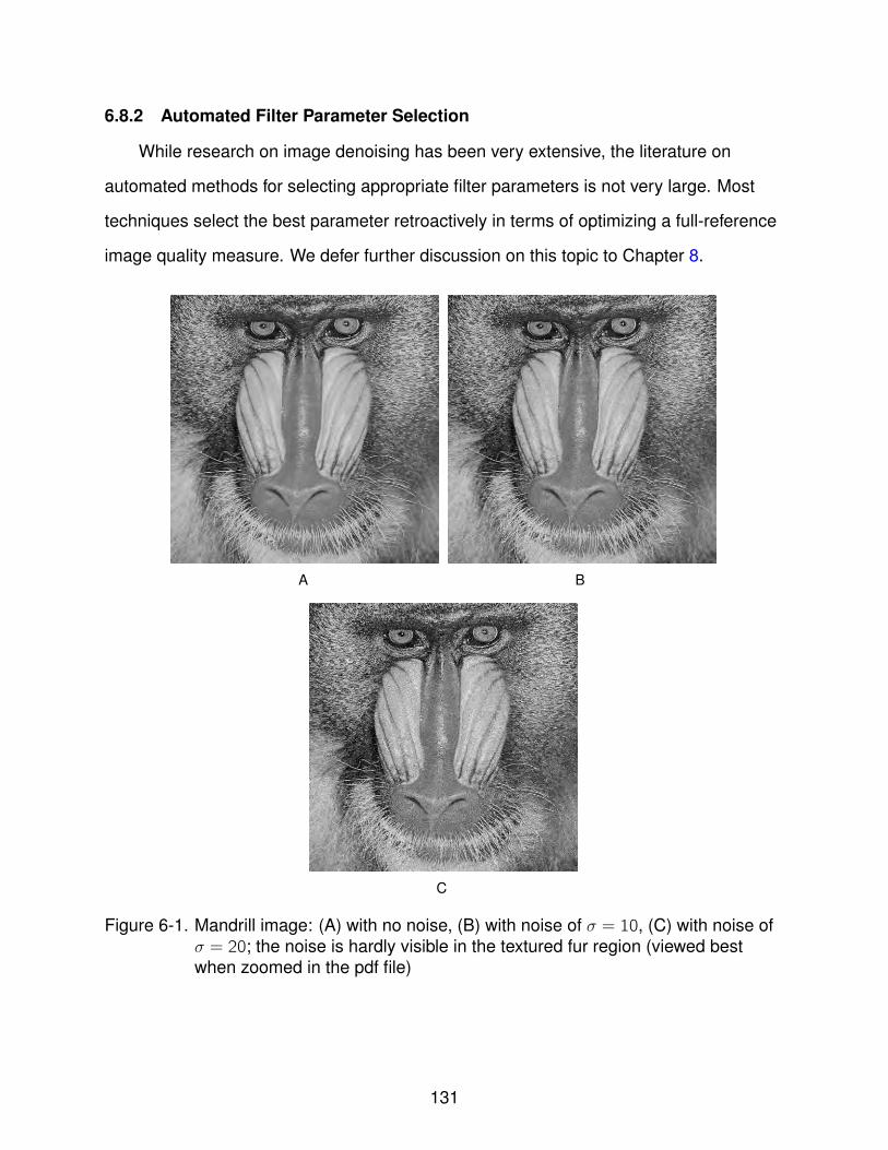
6.8.2 Automated Filter Parameter Selection
While research on image denoising has been very extensive, the literature on
automated methods for selecting appropriate filter parameters is not very large. Most
techniques select the best parameter retroactively in terms of optimizing a full-reference
image quality measure. We defer further discussion on this topic to Chapter 8.
A B
C
Figure 6-1. Mandrill image: (A) with no noise, (B) with noise of σ = 10, (C) with noise ofσ = 20; the noise is hardly visible in the textured fur region (viewed bestwhen zoomed in the pdf file)
131

CHAPTER 7BUILDING UPON THE SINGULAR VALUE DECOMPOSITION FOR IMAGE
DENOISING
7.1 Introduction
This chapter describes two new algorithms for gray-scale image denoising. Our
methods are largely based upon the classical technique of singular value decomposition
(SVD), a popular concept in linear algebra. The SVD was first applied for image
filtering and compression applications in [152] and [153]. On a stand-alone basis, its
performance on filtering leaves much to be desired. However during this thesis, we
have explored several ideas which build upon the SVD, leading to simple and elegant
techniques with excellent performance. Many of the intermediate ideas that were
explored, failed to produce good results in terms of denoising performance. While the
vast majority of contemporary research literature focuses only on positive results, we
choose to adopt a different philosophy. We shall present negative results (and wherever
possible, analyze the reasons for the negative results) in addition to the positive ones
that are on par or better than the state of the art. We hope that this will provide readers
of this thesis with better insight and open up ideas for future research.
We observe that a principled denoising technique can be motivated by the following
considerations. What constitutes a good model for the images being dealt with? What
is known about the noise model? What properties distinguish a clean image from
one containing pure noise? We make the following assumptions in the theoretical
description and experimental results. We assume a gray-scale image in the intensity
range [0, 255] defined on a discrete rectangular domain Ω. In the techniques that we
investigate, we exploit different well-known properties of natural images. We assume
a zero mean i.i.d. (independent and identically distributed) Gaussian noise model of a
fixed standard deviation σ, as the common degradation process. We do not cover the
case of signal-dependent noise or those without precise probabilistic characteristics
(such as noise induced by lossy compression algorithms) in this thesis.
132
7.2 Matrix SVD
The matrix SVD is a popular technique in linear algebra with a wide variety of
applications in signal processing, such as filtering, compression and least-squares
regression to name a few. Given a matrix A of size m × n defined on the field of real
numbers, there always exists a factorization of the following form [154]
A = USV T (7–1)
where U is a m × m orthonormal matrix, S is a m × n diagonal matrix of positive
‘singular’ values and V is a n × n orthonormal matrix. Conventionally, the entries of S
are arranged in descending order of magnitude. Moreover, if the singular values happen
to be unique, the matrix SVD is always unique, modulo sign changes on the columns of
U and V . The columns of V (called the right singular vectors) are the eigenvectors of
ATA, whereas the columns of U (called the left singular vectors) are the eigenvectors of
AAT and the singular values in S turn out to be the square roots of the eigenvalues of
ATA (equivalently AAT ). A geometric interpretation of the SVD (assuming real vector
spaces) is presented in [154]. The matrix SVD has beautiful mathematical properties
such as providing a principled method for the nearest orthonormal matrix, and the best
lower-rank approximation to a matrix (both in the sense of the Frobenius norm) [154].
7.3 SVD for Image Denoising
It is well-known that the singular values of natural images follow an exponential
decay rule [155]. This property also holds true for Fourier coefficient magnitudes. In
fact, the SVD bases have a frequency interpretation. The smaller singular values of the
image correspond to higher frequencies and the large values correspond to the lower
frequency components. This property of the SVD has been used both in denoising [152]
as well as in compression [153].
Now, consider a noisy image A (a degraded version of an underlying clean
image Ac ) affected by additive Gaussian noise of standard deviation σ. Filtering is
133
accomplished by computing the decomposition A = USV T and then nullifying the
smaller values of A, which effectively discards higher frequency components (which are
known to correspond mostly to noise) [152]. An example of this procedure is illustrated
in Figure 7-1, where all singular values smaller than some k th singular value were set to
zero. It is clearly seen that low rank truncation (i.e. if the index k is chosen to be small)
produces blurry images and increasing the rank adds in image details but introduces
more and more noise. Taking this sub-par performance into account, this decomposition
is instead performed at the level of image patches. Indeed, small patches capture local
information which can be compactly represented with small-sized bases. The SVD is
computed in a sliding window fashion and filtered versions of overlapping patches are
averaged in order to produce a final filtered image. The averaging is useful for removing
seam artifacts at patch boundaries and also brings in multiple hypotheses. These results
are shown in Figure 7-2 for different settings: (1) rank 1 and rank 2 truncation of each
patch, (2) nullification of patch singular values below a fixed threshold of σ√2 logN
(where N is the number of image pixels), and (3) truncation of singular values in such
a way that the residual at each patch has a standard deviation of σ (i.e. a standard
deviation equal to that of the noise).
7.4 Oracle Denoiser with the SVD
Despite the improvement in results with the patch-based method (as seen upon
comparing Figures 7-2 and 7-1), the filtering performance is still far from desirable.
The main reason for this is that the singular vectors are unable to adequately separate
signal from noise. There are two key observations we make here. Firstly, let Q and
Qn be corresponding patches from a clean image and its noisy version respectively.
Given the decomposition Qn = UnSnV Tn , the projection of Q (the true patch) onto the
bases (Un,Vn) is given as SQ = UTn QVn. This matrix SQ is non-diagonal and hence
contains more non-zero elements than Sn. Note the fact that SQ is ‘denser’ than Sn.
Despite this, if we could somehow change the entries in Sn to match those in SQ , we
134
would now have a perfect denoising technique. Nevertheless, SVD-based filtering
techniques emphasize low-rank truncation or other methods of increasing the sparsity
of the matrix of singular values. We shall dwell more on this point in Section 7.5 in
the context of filtering with SVD bases as well as universal bases such as the DCT.
The second important observation is that the additive noise doesn’t just affect the
singular values of the patch but the singular vectors (which are the eigenvectors of the
row-row and column-column correlation matrices of the patch) as well. Bearing this in
mind, it is strange that SVD-based denoising techniques do not seek to manipulate the
orthonormal bases and instead focus only on changing the singular values. We now
perform the following experiment which starts with a noisy image and assumes that
the true singular vectors of the clean patch underlying every noisy patch in the image
are known or provided to us by an oracle. The denoising technique now proceeds as
follows:
1. Let the SVD for a patch Q(i) from a clean image be Q(i) = USV T . Project the noisypatch Q(i)n onto these bases to produce a matrix SQ(i) = UTQ(i)V .
2. Set to zero all elements in SQ(i) such that |SQ(i)| < λσ.
3. Produce the denoised version of Q(i)n by inverting the projection.
4. Repeat the above procedure in sliding window fashion and average all thehypotheses at every pixel to yield a denoised image.
We term this method as the ‘oracle denoiser’. Given 8 × 8 patches, we choose the
threshold of λ = 3 for the following reasons. Firstly, zero mean Gaussian random
variables with standard deviation σ (i.e. belonging to N (0,σ)) have value less than 3σ
with high probability, and projections of matrices of Gaussian random variables onto
orthonormal bases also obey this rule (experimentally, this probability was observed to
be very close to 1). Secondly, λ = 3 comes close to the idea threshold of λ =√2 log n2
from [113] for patches of size n × n.
135

Sample experimental results with the above technique are shown in Figure 7-3
for two noise levels: 20 and 40. The resulting PSNR values of this ideal denoiser far
exceed the state of the art methods such as BM3D [134]. Clearly, this experiment is
not possible in practice, however it serves as a benchmark, drives home an important
deficiency of contemporary SVD filtering approaches, and chalks out a path for us to
explore: manipulating the SVD bases of a noisy patch, or somehow using bases that are
‘better’ than the SVD bases of the noisy patch, may be the key to improving denoising
performance.
7.5 SVD, DCT and Minimum Mean Squared Error Estimators
As has been described in Section 6.4, nullification of the smaller coefficient values
from the projection of a noisy patch onto a basis is actually a MAP estimator of the
coefficients of the true patch. The MAP estimator is driven by sparsity-promoting image
priors which hold for image ensembles but not necessarily for every individual image.
We therefore explore minimum mean square error (MMSE) estimators for estimation of
the true projection coefficients.
7.5.1 MMSE Estimators with DCT
The idea of using MMSE estimators is inspired by the work in [120]. However, there
is one major difference between the approach from [120] and the one we present here.
In [120], the authors learn a generic rule to optimally perturb the DCT coefficients of
an ensemble of noisy image patches so as to reduce the mean squared error with the
DCT coefficients of their corresponding underlying clean patches. A different rule is
learned for each DCT coefficient (the number of coefficients is equal to the patch-size)
or for each sub-band, though all the rules are common across patches. However, we
have observed experimentally that the optimal rules for patches of different geometric
structures differ significantly from one another (see Figure 7-5). Therefore, we move
away from the notion of a single set of rules for the entire ensemble and instead learn
a different set of rules for each training patch. We make the definition of the word ‘rule’
136
more precise in the following. Consider the i th patch from a database PD of N patches.
We shall denote the patch as Ii . Let its size be n × n and let its k th DCT coefficient be
Ii(k)
where 1 ≤ k ≤ n2. Let us denote Jij as the j th noisy instance of patch Ii where
1 ≤ j ≤ M, and let Jij(k)
be its k th DCT coefficient. Then for each 1 ≤ k ≤ n2 and for
each patch 1 ≤ i ≤ N, we may seek a perturbation εki such that
εki = minε
M∑j=1
(Jij(k)+ ε− Ii
(k))2. (7–2)
Unfortunately, the values of corresponding DCT coefficients belonging to multiple noisy
instances of a patch show considerable variance, which prevents the learning of any
meaningful perturbation rule. To alleviate this problem, we quantize the values of each
DCT coefficient into a fixed number of bins, say B. Thus for the k th coefficient of the i th
patch, we no more learn a single scalar value, but a set of B perturbation values εkib,
one for each bin. This can be mathematically expressed as
εkib = minε
M∑j=1
δb(Jij(k))(Jij
(k)+ ε− Ii
(k))2 (7–3)
where
δb(Jij(k)) =
1 if bm(1)ik −m(2)ikB
c = b
0 otherwise.(7–4)
In the above equation, we define the following terms:
m(1)ik = maxj Jij
(k)(7–5)
m(2)ik = minj Jij
(k). (7–6)
Note that the quantization of the coefficients is motivated by the fact that the perturbation
of the coefficients owing to corruption by Gaussian noise shows some regularity, since
random variables from N (0,σ) lie within a bounded interval [−3σ, +3σ] with very high
probability.
137
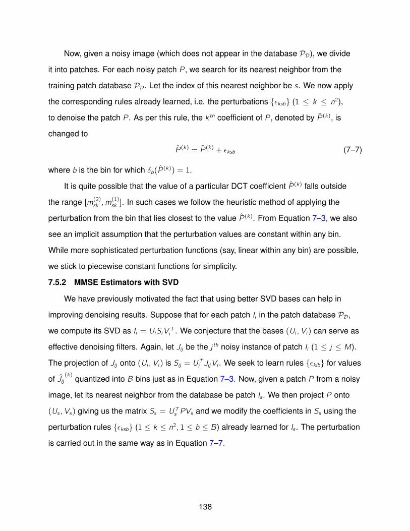
Now, given a noisy image (which does not appear in the database PD), we divide
it into patches. For each noisy patch P, we search for its nearest neighbor from the
training patch database PD. Let the index of this nearest neighbor be s. We now apply
the corresponding rules already learned, i.e. the perturbations εksb (1 ≤ k ≤ n2),
to denoise the patch P. As per this rule, the k th coefficient of P, denoted by P(k), is
changed to
P(k) = P(k) + εksb (7–7)
where b is the bin for which δb(P(k)) = 1.
It is quite possible that the value of a particular DCT coefficient P(k) falls outside
the range [m(2)sk ,m(1)sk ]. In such cases we follow the heuristic method of applying the
perturbation from the bin that lies closest to the value P(k). From Equation 7–3, we also
see an implicit assumption that the perturbation values are constant within any bin.
While more sophisticated perturbation functions (say, linear within any bin) are possible,
we stick to piecewise constant functions for simplicity.
7.5.2 MMSE Estimators with SVD
We have previously motivated the fact that using better SVD bases can help in
improving denoising results. Suppose that for each patch Ii in the patch database PD,
we compute its SVD as Ii = UiSiV Ti . We conjecture that the bases (Ui ,Vi) can serve as
effective denoising filters. Again, let Jij be the j th noisy instance of patch Ii (1 ≤ j ≤ M).
The projection of Jij onto (Ui ,Vi) is Sij = UTi JijVi . We seek to learn rules εkib for values
of Jij(k)
quantized into B bins just as in Equation 7–3. Now, given a patch P from a noisy
image, let its nearest neighbor from the database be patch Is . We then project P onto
(Us ,Vs) giving us the matrix Ss = UTs PVs and we modify the coefficients in Ss using the
perturbation rules εksb (1 ≤ k ≤ n2, 1 ≤ b ≤ B) already learned for Is . The perturbation
is carried out in the same way as in Equation 7–7.
138
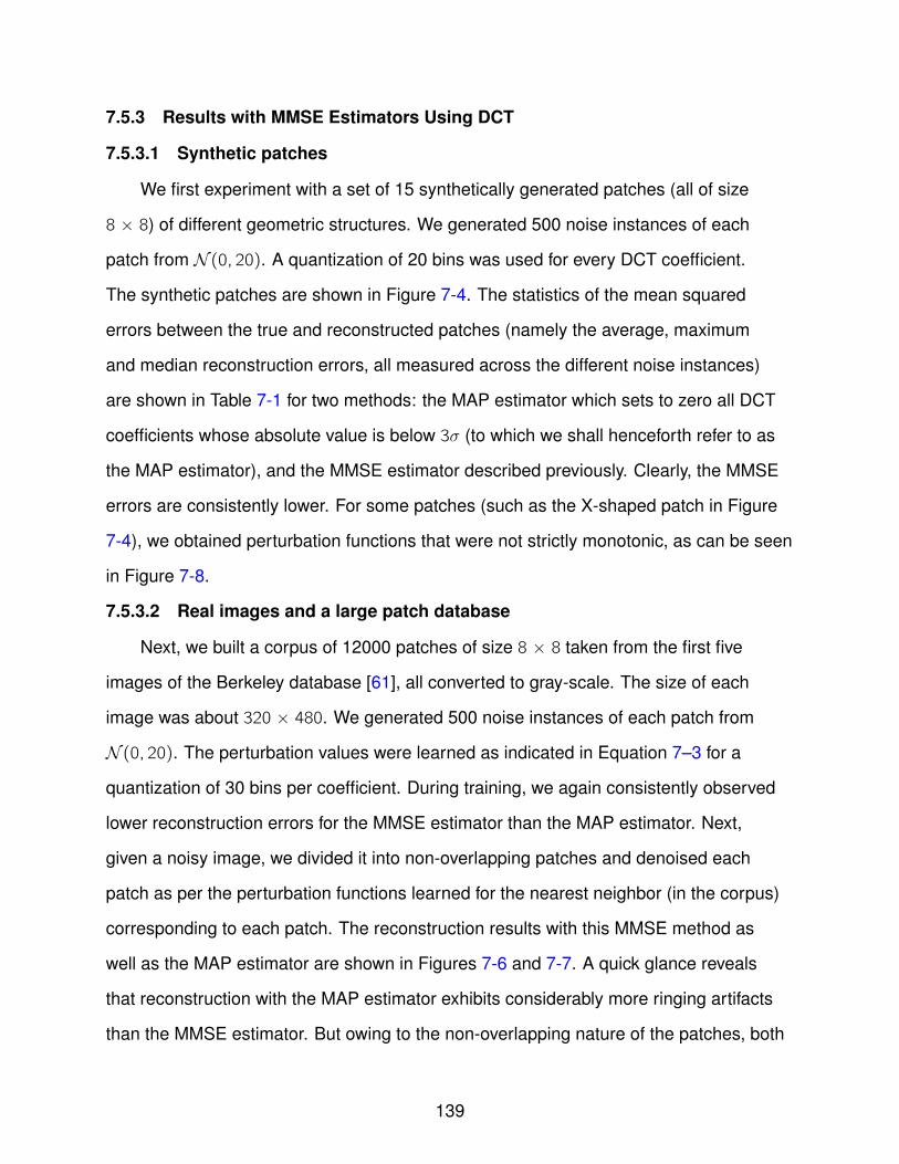
7.5.3 Results with MMSE Estimators Using DCT
7.5.3.1 Synthetic patches
We first experiment with a set of 15 synthetically generated patches (all of size
8 × 8) of different geometric structures. We generated 500 noise instances of each
patch from N (0, 20). A quantization of 20 bins was used for every DCT coefficient.
The synthetic patches are shown in Figure 7-4. The statistics of the mean squared
errors between the true and reconstructed patches (namely the average, maximum
and median reconstruction errors, all measured across the different noise instances)
are shown in Table 7-1 for two methods: the MAP estimator which sets to zero all DCT
coefficients whose absolute value is below 3σ (to which we shall henceforth refer to as
the MAP estimator), and the MMSE estimator described previously. Clearly, the MMSE
errors are consistently lower. For some patches (such as the X-shaped patch in Figure
7-4), we obtained perturbation functions that were not strictly monotonic, as can be seen
in Figure 7-8.
7.5.3.2 Real images and a large patch database
Next, we built a corpus of 12000 patches of size 8 × 8 taken from the first five
images of the Berkeley database [61], all converted to gray-scale. The size of each
image was about 320 × 480. We generated 500 noise instances of each patch from
N (0, 20). The perturbation values were learned as indicated in Equation 7–3 for a
quantization of 30 bins per coefficient. During training, we again consistently observed
lower reconstruction errors for the MMSE estimator than the MAP estimator. Next,
given a noisy image, we divided it into non-overlapping patches and denoised each
patch as per the perturbation functions learned for the nearest neighbor (in the corpus)
corresponding to each patch. The reconstruction results with this MMSE method as
well as the MAP estimator are shown in Figures 7-6 and 7-7. A quick glance reveals
that reconstruction with the MAP estimator exhibits considerably more ringing artifacts
than the MMSE estimator. But owing to the non-overlapping nature of the patches, both
139
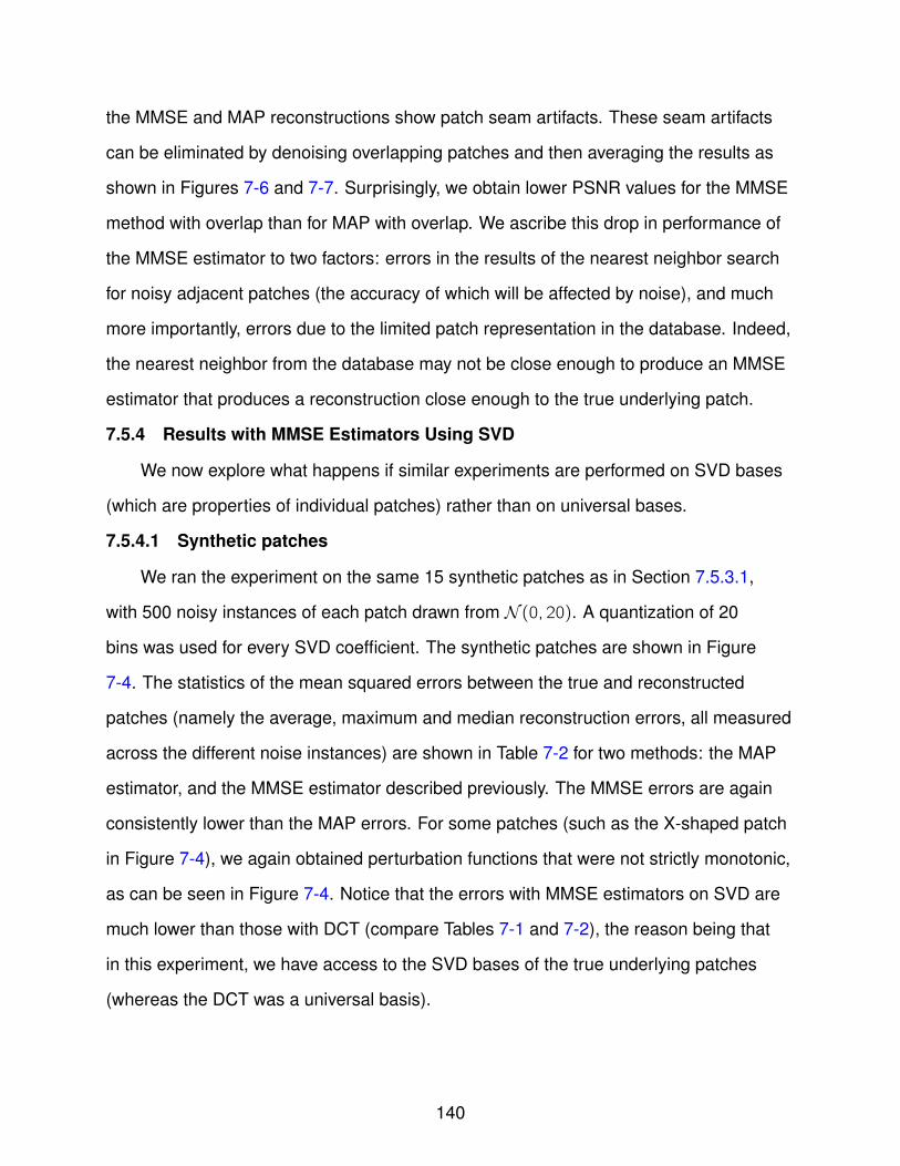
the MMSE and MAP reconstructions show patch seam artifacts. These seam artifacts
can be eliminated by denoising overlapping patches and then averaging the results as
shown in Figures 7-6 and 7-7. Surprisingly, we obtain lower PSNR values for the MMSE
method with overlap than for MAP with overlap. We ascribe this drop in performance of
the MMSE estimator to two factors: errors in the results of the nearest neighbor search
for noisy adjacent patches (the accuracy of which will be affected by noise), and much
more importantly, errors due to the limited patch representation in the database. Indeed,
the nearest neighbor from the database may not be close enough to produce an MMSE
estimator that produces a reconstruction close enough to the true underlying patch.
7.5.4 Results with MMSE Estimators Using SVD
We now explore what happens if similar experiments are performed on SVD bases
(which are properties of individual patches) rather than on universal bases.
7.5.4.1 Synthetic patches
We ran the experiment on the same 15 synthetic patches as in Section 7.5.3.1,
with 500 noisy instances of each patch drawn from N (0, 20). A quantization of 20
bins was used for every SVD coefficient. The synthetic patches are shown in Figure
7-4. The statistics of the mean squared errors between the true and reconstructed
patches (namely the average, maximum and median reconstruction errors, all measured
across the different noise instances) are shown in Table 7-2 for two methods: the MAP
estimator, and the MMSE estimator described previously. The MMSE errors are again
consistently lower than the MAP errors. For some patches (such as the X-shaped patch
in Figure 7-4), we again obtained perturbation functions that were not strictly monotonic,
as can be seen in Figure 7-4. Notice that the errors with MMSE estimators on SVD are
much lower than those with DCT (compare Tables 7-1 and 7-2), the reason being that
in this experiment, we have access to the SVD bases of the true underlying patches
(whereas the DCT was a universal basis).
140
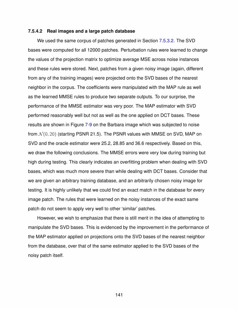
7.5.4.2 Real images and a large patch database
We used the same corpus of patches generated in Section 7.5.3.2. The SVD
bases were computed for all 12000 patches. Perturbation rules were learned to change
the values of the projection matrix to optimize average MSE across noise instances
and these rules were stored. Next, patches from a given noisy image (again, different
from any of the training images) were projected onto the SVD bases of the nearest
neighbor in the corpus. The coefficients were manipulated with the MAP rule as well
as the learned MMSE rules to produce two separate outputs. To our surprise, the
performance of the MMSE estimator was very poor. The MAP estimator with SVD
performed reasonably well but not as well as the one applied on DCT bases. These
results are shown in Figure 7-9 on the Barbara image which was subjected to noise
from N (0, 20) (starting PSNR 21.5). The PSNR values with MMSE on SVD, MAP on
SVD and the oracle estimator were 25.2, 28.85 and 36.6 respectively. Based on this,
we draw the following conclusions. The MMSE errors were very low during training but
high during testing. This clearly indicates an overfitting problem when dealing with SVD
bases, which was much more severe than while dealing with DCT bases. Consider that
we are given an arbitrary training database, and an arbitrarily chosen noisy image for
testing. It is highly unlikely that we could find an exact match in the database for every
image patch. The rules that were learned on the noisy instances of the exact same
patch do not seem to apply very well to other ‘similar’ patches.
However, we wish to emphasize that there is still merit in the idea of attempting to
manipulate the SVD bases. This is evidenced by the improvement in the performance of
the MAP estimator applied on projections onto the SVD bases of the nearest neighbor
from the database, over that of the same estimator applied to the SVD bases of the
noisy patch itself.
141
7.6 Filtering of SVD Bases
We have observed that the SVD bases of adjacent patches (i.e. patches with their
top-left corners at adjacent pixels) from clean natural images tend to exhibit greater
similarity than those from noisy versions of those images. The similarity is quantified in
terms of the angles between unit vectors from corresponding columns of the U matrices
(or those of the V matrices) of the adjacent patches. This observation is clearly a
property of natural image patches (and not a mere consequence of the fact that we
computed SVD bases of matrices that had several rows or columns in common). With
this in mind, we explored the effect of smoothing the U and V bases of adjacent patches
from the image using some averaging techniques. There are three ways this could be
done:
1. Smooth (say by some sort of averaging scheme) the corresponding columns fromthe U matrices of adjacent patches, and the corresponding columns from the Vmatrices of adjacent patches.
2. Smooth (say by some sort of averaging scheme) the outer products UiV Ti (1 ≤ i ≤n, 1 ≤ j ≤ n), i.e. outer products of the corresponding columns from the U and Vbases computed from adjacent patches.
3. Run a diffusion PDE defined specifically for orthonormal matrices on the U basesand also on the V bases (independently).
There are mathematical complications that arise in the first method: the averaging really
ought to be done by respecting the geometry of the space of orthonormal matrices.
However, the orthonormal matrices with determinant +1 are disjoint from those with
determinant -1. This is problematic from the point of view of computing intrinsic
averages. Furthermore, independent averaging of the U and V matrices ignores the
inherent coupling between them (as given a patch P, they are eigenvectors of PTP and
PPT respectively). Taking averages of outer products of corresponding columns from U
and V helps bring in this dependence. However, it still ignores the dependence between
the different outer products themselves.
142

Ignoring the above mathematical issues, we computed Euclidean averages. As the
resultant matrices were no more orthonormal, we orthonormalized them using a QR
decomposition. While computing averages of outer products (in method 2), there are
considerable complications in forcing the averaged outer-product to lie in the space of
matrices of the form v1vT2 where |v1| = |v2| = 1, which were ignored in our experiments.
We performed image denoising experiments by first smoothing the bases computed
from 8 × 8 patches using either of the three techniques, projecting the patches onto
the bases, applying the MAP rule on the coefficients of the projection matrix and
reconstructing the patch by inverting the transform. In case of the diffusion PDE defined
for orthonormal matrices, we used the following isotropic heat equation defined in [156]
for matrix U ∈ SO(p × p):dUk
dt= −Lk +
p∑i=1
(Li .Uk)U i (7–8)
where
Lk = Ukxx + Ukyy (7–9)
and Uk stands for the k th column of U.
Note that coupling between the U and V matrices can be imposed indirectly by
introduction of a data fidelity constraint on the patch P in addition to the smoothness
term on the U and V matrices, and then executing alternating PDEs (Euler-Lagrange
equations) on U and V . However, experimental results on averaging of the SVD bases
were in general not satisfactory. Similar experiments were repeated with nonlocal
averaging of similar U and V matrices from different regions of the image, and there was
no improvement in the results. We conjecture that the smoothness of U and V bases
from adjacent patches may not be a strong enough property of natural images.
7.7 Nonlocal SVD with Ensembles of Similar Patches
We now present an algorithm for image denoising using a non-local extension of the
SVD. We call this algorithm non-local SVD or NL-SVD.
143
We know that the SVD of a matrix P ∈ Rm×n is given as P = USV T where the
columns of U consist of the eigenvectors of the matrix
Cr = PPT (7–10)
where the element of Cr from the i th row and j th column is given as
Crij =∑k
PikPjk =< Pi ,Pj > (7–11)
where Pi and Pj stand for the i th and j th rows of P respectively. Similarly the columns of
V consist of the eigenvectors of the matrix
Cc = PPT (7–12)
where the element of Cc from the i th row and j th column is given as
Ccij =∑k
PkiPkj =< PTi ,P
Tj > (7–13)
where PTi and PTj stand for the i th and j th columns of P respectively. Note that Cr and
Cc are the row-row and column-column correlation matrices of P respectively. We also
know that the SVD gives us the optimal low-rank decomposition of P. In other words, the
optimal solution to
E(P) = ‖P − P‖2 (7–14)
subject to the constraint
rank(P) = k k < m, k < n (7–15)
is given by
P = ‖Uk SV Tk ‖2 (7–16)
where Uk and Vk are the first k columns of U and V respectively and S contains the k
largest singular values of S . This is often called as the Eckhart-Young theorem [154].
144
Given the inadequate performance of the local patch SVD, we continue our search
for ‘better’ bases to represent each patch. With this in mind, we now explore what would
happen if we were to consider a non-local generalization of the SVD. Given a patch P
from the noisy image, we look for other patches in the image that are ‘similar’ to P. We
will give a precise definition of similarity later in Section 7.7.1. Let us consider that there
are K such similar patches (including P) which we label as Pi where 1 ≤ i ≤ K .
Next, we ask the following question: what single pair of orthonormal matrices Uk and Vk
will provide the best rank-k approximation to all the patches Pi? In other words, what
(Uk ,Vk) minimizes the following energy?
E(Uk , Si,Vk) =K∑i=1
‖Pi − UkSiV Tk ‖2 (7–17)
where
UTk Uk = I (7–18)
V Tk Vk = I (7–19)
∀i ,Si ∈ Rk×k . (7–20)
The solution to this problem is given by an iterative minimization (starting from random
initial conditions) presented in [157]. Note that the matrices Si in this case are not
diagonal. Note also that the basis Uk ,Vk does not correspond to the individual SVD
bases but to a basis pair that is common to all the chosen patches. Related work in
[155] presents an alternating minimization framework with the additional (heuristically
driven) constraint that all the matrices Si are diagonal. This constraint is imposed at
every step of the alternating minimization framework. An approximate solution to the
energy function in Equation 7–17 is presented in [158]. This solution, which is called
as the 2D-SVD, can be computed in closed form and obviates the need for expensive
iterative optimizations. The 2D-SVD for the patch collection Pi is given as follows.
145

Consider the row-row and column-column correlation matrices
Cr =
K∑i=1
PiPTi (7–21)
Cc =
K∑i=1
PTi Pi . (7–22)
Then Uk contains the first k eigenvectors of Cr corresponding to the k largest eigenvalues
of Cr , and Vk contains the first k eigenvectors of Cc corresponding to the k largest
eigenvalues of Cc . The precise error bounds for the approximate solution w.r.t. the true
global solution are derived in [158].
We use this non-local SVD framework in a denoising algorithm and we shall show
later that this produces results competitive with the start of the art. We start off by
dividing the given noisy image into patches. For each ‘reference’ patch, we collect
patches similar to it and obtain the common basis for them using the non-local SVD
method. However, this leaves open the problem of deciding on the best rank k for the
bases, which need not be constant across patches of different geometric structure.
We obviate the need for selection of this parameter by following a different approach.
We compute the full-rank orthonormal bases U and V , i.e. we choose k = n for n × n
patches. Now the given noisy patch P is projected onto the pair (U,V ) producing the
matrix S (P) = UTPV . Essentially, we can write the entries of P as
Pij =∑kl
S(P)kl UkiVlj (7–23)
which is equivalent to a linear combination of outer products of the form UkV Tl (1 ≤ k ≤
n, 1 ≤ l ≤ n). We conjecture that this formulation has an interpretation in terms of 2D
spatial frequencies wherein the smaller coefficient values correspond to higher values
of at least one of the frequencies. Therefore, we choose to nullify the coefficients with
smaller values (as decided by a threshold). Given such a ‘filtered’ projection matrix S (P),
we reconstruct the patch. This operation is repeated on overlapping patches in a sliding
146
window fashion and the overlapping hypotheses are aggregated by averaging leading to
a final filtered image. Crucial to the performance of this filter is the choice of a notion of
patch similarity and also the choice of thresholds for removing smaller coefficients. We
discuss these choices below.
7.7.1 Choice of Patch Similarity Measure
Given a reference patch P ref in a noisy image, we can compute its K nearest
neighbors from the image, but this requires a choice of K which may not be the same
across different image patches. Hence, we revert to a distance threshold τd and select
all patches Pi such that the total squared difference between P ref and Pi is below τd .
Note that we have throughout assumed a fixed and known noise model - N (0,σ). If we
were to assume that P ref and Pi were different noisy versions of the same underlying
patch, we observe that the following random variable has a χ2 density with z = n2
degrees of freedom:
x =
n2∑k=1
(P refk − Pik)2
2σ2. (7–24)
The cumulative of a χ2 random variable with z degrees of freedom is given by the
expression
F (x ; z) = γ(x
2,z
2) (7–25)
where γ(x , a) stands for the incomplete gamma function defined as follows:
γ(x , a) =1
Γ(a)
∫ xt=0
e−tta−1dt (7–26)
with Γ(a) being the Gamma function defined as
Γ(a) =
∫ ∞
0
e−tt(a−1)dt. (7–27)
We observe that if z ≥ 3, for any x ≥ 3z , we have F (x ; z) ≥ 0.99. Therefore for a
patch-size of n × n and under the given σ, we choose the following threshold for the total
147
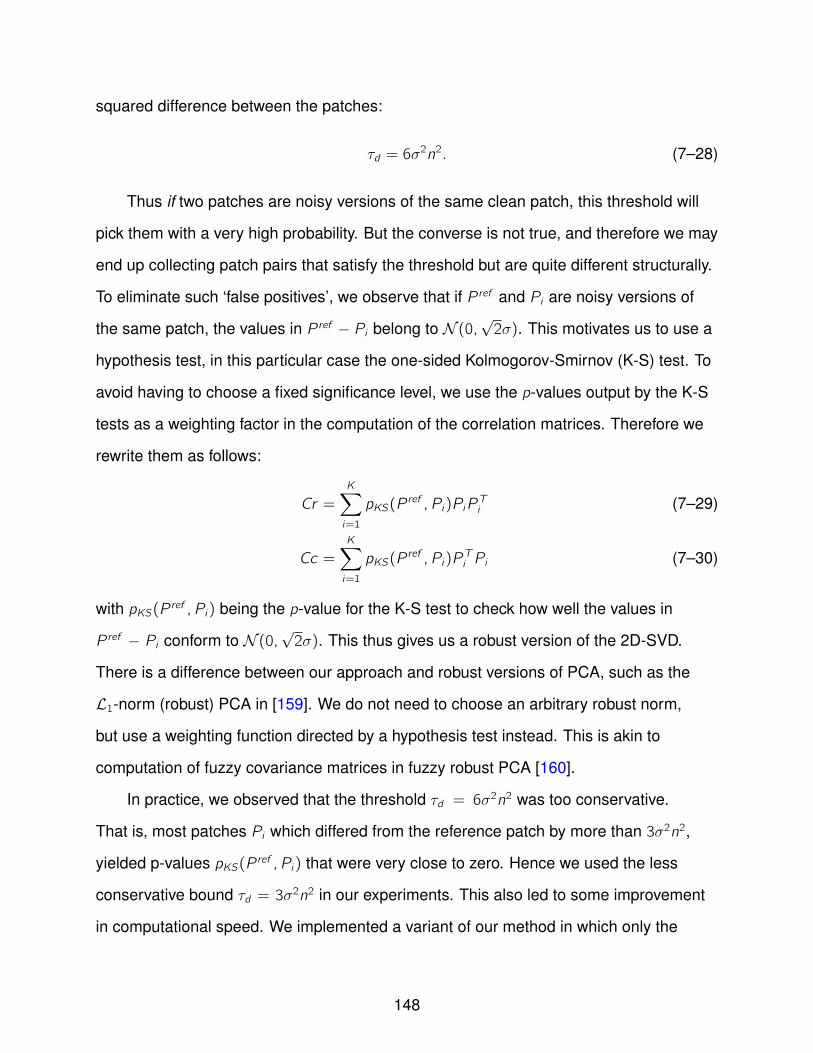
squared difference between the patches:
τd = 6σ2n2. (7–28)
Thus if two patches are noisy versions of the same clean patch, this threshold will
pick them with a very high probability. But the converse is not true, and therefore we may
end up collecting patch pairs that satisfy the threshold but are quite different structurally.
To eliminate such ‘false positives’, we observe that if P ref and Pi are noisy versions of
the same patch, the values in P ref − Pi belong to N (0,√2σ). This motivates us to use a
hypothesis test, in this particular case the one-sided Kolmogorov-Smirnov (K-S) test. To
avoid having to choose a fixed significance level, we use the p-values output by the K-S
tests as a weighting factor in the computation of the correlation matrices. Therefore we
rewrite them as follows:
Cr =
K∑i=1
pKS(Pref ,Pi)PiP
Ti (7–29)
Cc =
K∑i=1
pKS(Pref ,Pi)P
Ti Pi (7–30)
with pKS(P ref ,Pi) being the p-value for the K-S test to check how well the values in
P ref − Pi conform to N (0,√2σ). This thus gives us a robust version of the 2D-SVD.
There is a difference between our approach and robust versions of PCA, such as the
L1-norm (robust) PCA in [159]. We do not need to choose an arbitrary robust norm,
but use a weighting function directed by a hypothesis test instead. This is akin to
computation of fuzzy covariance matrices in fuzzy robust PCA [160].
In practice, we observed that the threshold τd = 6σ2n2 was too conservative.
That is, most patches Pi which differed from the reference patch by more than 3σ2n2,
yielded p-values pKS(P ref ,Pi) that were very close to zero. Hence we used the less
conservative bound τd = 3σ2n2 in our experiments. This also led to some improvement
in computational speed. We implemented a variant of our method in which only the
148

threshold τd was used for patch selection, and the hypothesis test was entirely ignored.
Surprisingly, we did not experience any significant drop in performance on our datasets
if the hypothesis test was neglected. Nonetheless in all reported results, we still used
the hypothesis test because it is a principled way of mitigating the effect of false
positives. An example of the phenomenon of false positives is illustrated in Figure
7-10. The two images in Figure 7-10 are structurally very different (containing graylevels
of 10 and 40), and yet the MSE between their noisy versions (σ = 20) is only 4075 which
falls below the threshold of 3σ2 = 4800. However the KS-test yields a p-value very close
to 0, thereby providing a better indication of structural dissimilarity.
It should be further noted that even the bound τd ≤ 3σ2n2 is quite conservative. It
can be refined using the fact that the χ2 density can be approximated as N (n2, n√2) if
n2 is large. This results follows from the central limit theorem and holds good for n2 ≥ 64.
This gives us the following refined bound:
τd = (n2 +
√2× 2.362n)2σ2 = 2(n2 + 3.29n)σ2 (7–31)
from the inverse cumulative for N (n2,√2n) at 0.99.
7.7.2 Choice of Threshold for Truncation of Transform Coefficients
As our noise model is N (0,σ), we observe that the corresponding random variables
in n × n patches have magnitude less than σ√2 log n2 with very high probability,
as also the entries of the corresponding projection matrices (onto orthonormal
bases/basis-pairs). Hence we assume that coefficients less than this threshold have
been produced due to noise. This threshold happens to be the universally optimal
threshold for wavelet denoising with hard thresholding [113] (also see Section 6.4), and
holds specifically for i.i.d. Gaussian noise for any given orthonormal basis. While hard
thresholding may lead to elimination of some useful high-frequency information, this loss
is compensated through the redundancy from overlapping patches [108].
149
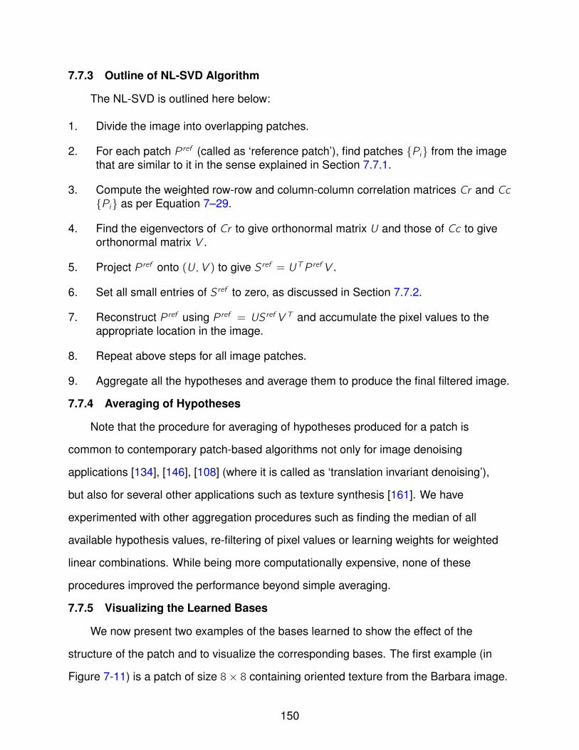
7.7.3 Outline of NL-SVD Algorithm
The NL-SVD is outlined here below:
1. Divide the image into overlapping patches.
2. For each patch P ref (called as ‘reference patch’), find patches Pi from the imagethat are similar to it in the sense explained in Section 7.7.1.
3. Compute the weighted row-row and column-column correlation matrices Cr and CcPi as per Equation 7–29.
4. Find the eigenvectors of Cr to give orthonormal matrix U and those of Cc to giveorthonormal matrix V .
5. Project P ref onto (U,V ) to give S ref = UTP refV .
6. Set all small entries of S ref to zero, as discussed in Section 7.7.2.
7. Reconstruct P ref using P ref = US refV T and accumulate the pixel values to theappropriate location in the image.
8. Repeat above steps for all image patches.
9. Aggregate all the hypotheses and average them to produce the final filtered image.
7.7.4 Averaging of Hypotheses
Note that the procedure for averaging of hypotheses produced for a patch is
common to contemporary patch-based algorithms not only for image denoising
applications [134], [146], [108] (where it is called as ‘translation invariant denoising’),
but also for several other applications such as texture synthesis [161]. We have
experimented with other aggregation procedures such as finding the median of all
available hypothesis values, re-filtering of pixel values or learning weights for weighted
linear combinations. While being more computationally expensive, none of these
procedures improved the performance beyond simple averaging.
7.7.5 Visualizing the Learned Bases
We now present two examples of the bases learned to show the effect of the
structure of the patch and to visualize the corresponding bases. The first example (in
Figure 7-11) is a patch of size 8× 8 containing oriented texture from the Barbara image.
150
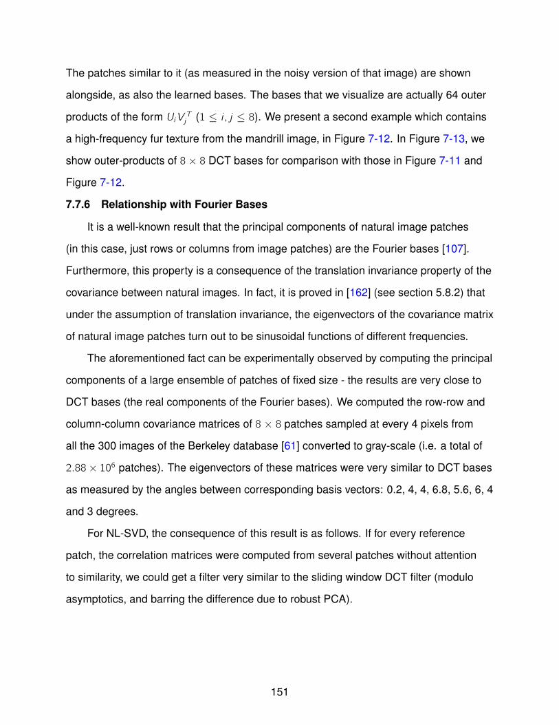
The patches similar to it (as measured in the noisy version of that image) are shown
alongside, as also the learned bases. The bases that we visualize are actually 64 outer
products of the form UiV Tj (1 ≤ i , j ≤ 8). We present a second example which contains
a high-frequency fur texture from the mandrill image, in Figure 7-12. In Figure 7-13, we
show outer-products of 8 × 8 DCT bases for comparison with those in Figure 7-11 and
Figure 7-12.
7.7.6 Relationship with Fourier Bases
It is a well-known result that the principal components of natural image patches
(in this case, just rows or columns from image patches) are the Fourier bases [107].
Furthermore, this property is a consequence of the translation invariance property of the
covariance between natural images. In fact, it is proved in [162] (see section 5.8.2) that
under the assumption of translation invariance, the eigenvectors of the covariance matrix
of natural image patches turn out to be sinusoidal functions of different frequencies.
The aforementioned fact can be experimentally observed by computing the principal
components of a large ensemble of patches of fixed size - the results are very close to
DCT bases (the real components of the Fourier bases). We computed the row-row and
column-column covariance matrices of 8 × 8 patches sampled at every 4 pixels from
all the 300 images of the Berkeley database [61] converted to gray-scale (i.e. a total of
2.88× 10⁶ patches). The eigenvectors of these matrices were very similar to DCT bases
as measured by the angles between corresponding basis vectors: 0.2, 4, 4, 6.8, 5.6, 6, 4
and 3 degrees.
For NL-SVD, the consequence of this result is as follows. If for every reference
patch, the correlation matrices were computed from several patches without attention
to similarity, we could get a filter very similar to the sliding window DCT filter (modulo
asymptotics, and barring the difference due to robust PCA).
151
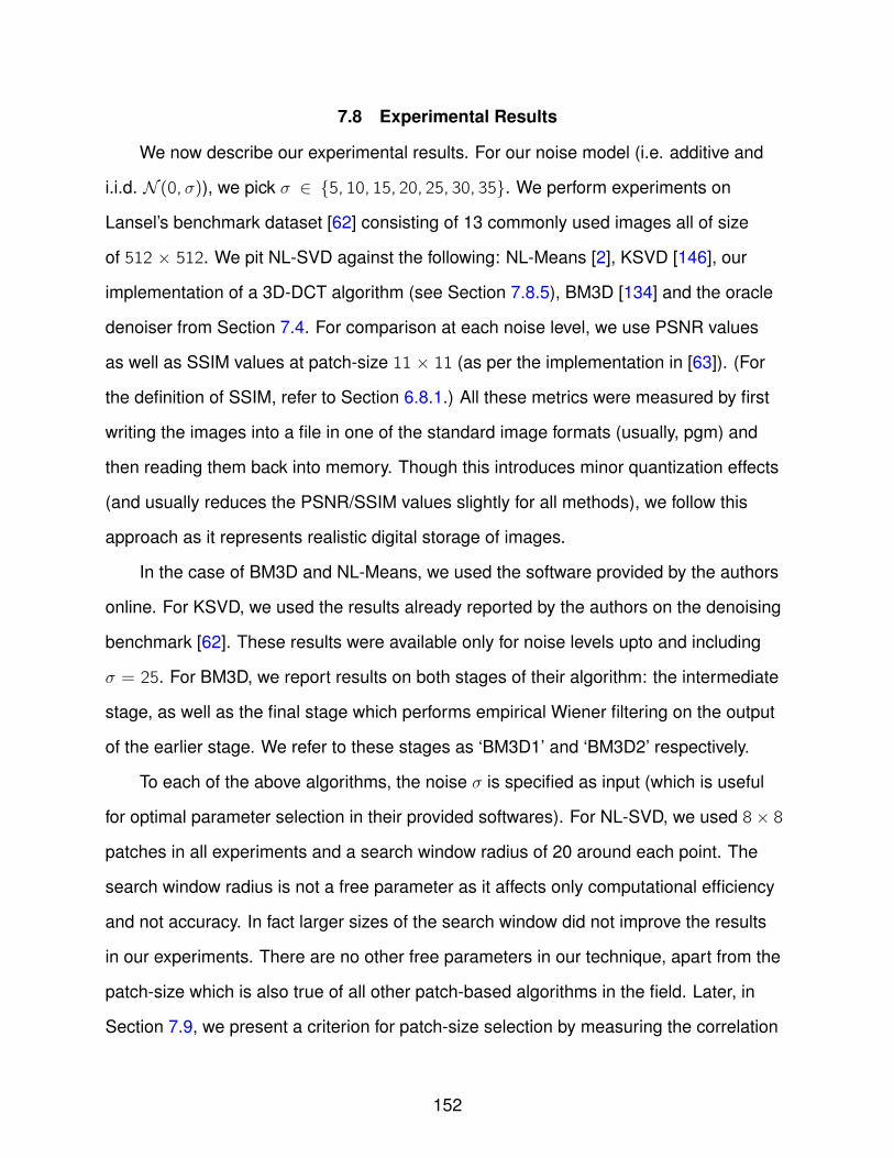
7.8 Experimental Results
We now describe our experimental results. For our noise model (i.e. additive and
i.i.d. N (0,σ)), we pick σ ∈ 5, 10, 15, 20, 25, 30, 35. We perform experiments on
Lansel’s benchmark dataset [62] consisting of 13 commonly used images all of size
of 512 × 512. We pit NL-SVD against the following: NL-Means [2], KSVD [146], our
implementation of a 3D-DCT algorithm (see Section 7.8.5), BM3D [134] and the oracle
denoiser from Section 7.4. For comparison at each noise level, we use PSNR values
as well as SSIM values at patch-size 11 × 11 (as per the implementation in [63]). (For
the definition of SSIM, refer to Section 6.8.1.) All these metrics were measured by first
writing the images into a file in one of the standard image formats (usually, pgm) and
then reading them back into memory. Though this introduces minor quantization effects
(and usually reduces the PSNR/SSIM values slightly for all methods), we follow this
approach as it represents realistic digital storage of images.
In the case of BM3D and NL-Means, we used the software provided by the authors
online. For KSVD, we used the results already reported by the authors on the denoising
benchmark [62]. These results were available only for noise levels upto and including
σ = 25. For BM3D, we report results on both stages of their algorithm: the intermediate
stage, as well as the final stage which performs empirical Wiener filtering on the output
of the earlier stage. We refer to these stages as ‘BM3D1’ and ‘BM3D2’ respectively.
To each of the above algorithms, the noise σ is specified as input (which is useful
for optimal parameter selection in their provided softwares). For NL-SVD, we used 8 × 8
patches in all experiments and a search window radius of 20 around each point. The
search window radius is not a free parameter as it affects only computational efficiency
and not accuracy. In fact larger sizes of the search window did not improve the results
in our experiments. There are no other free parameters in our technique, apart from the
patch-size which is also true of all other patch-based algorithms in the field. Later, in
Section 7.9, we present a criterion for patch-size selection by measuring the correlation
152

coefficient between patches from the residual image (i.e. difference between noisy and
denoised images). For NL-means, we used 9 × 9 patches throughout, with a search
window radius of 20. For BM3D implementation, we used the default settings of all the
various parameters as obtained from the authors’ software (their selected patch-size is
again 8 × 8). The results for KSVD have been reported by the authors themselves, and
hence we assume that the optimal parameter settings were already used for generating
those results.
7.8.1 Discussion of Results
From the PSNR results presented in Tables 7.12, 7.12, 7-7, 7-9, 7-12, 7-14 and
7-16, and the corresponding SSIM results in Tables 7-4, 7-6, 7-8, 7-10, 7-13, 7-15 and
7-17, we make several observations. NL-SVD is consistently superior to NL-Means in
terms of PSNR and SSIM. These tables also contain results of the HOSVD algorithm,
our second technique, which we shall be presenting later in Section 7.10. In all the
tables at the end of the chapter, we have used numbers to refer to image names to save
space. The numbers and the corresponding names are as follows: 13 - airplane, 12 -
Barbara, 11 - boats, 10 - couple, 9 - elaine, 8 - fingerprint, 7 - goldhill, 6 - Lena, 5 - man,
4 - mandrill, 3 - peppers, 2 - stream, 1 - Zelda.
7.8.2 Comparison with KSVD
Our PSNR and SSIM values are comparable to those reported for KSVD. However,
NL-SVD has several other advantages as compared to KSVD from a conceptual as well
as implementation point of view. KSVD learns an overcomplete dictionary on the fly
from the noisy image. This procedure requires iterated optimizations and is expensive.
The method is also prone to local minima and this puts artificial limits on the size of the
dictionary that should (or can) be learned [114]. The algorithm requires parameters that
are not easy to tune: the number of dictionary vectors (K ), parameter for the stopping
criterion for the pursuit projection algorithm and the tradeoff between data fidelity and
sparsity terms. On the other hand, NL-SVD derives a spatially adaptive basis at each
153
pixel in one step and requires no further iterations. Moreover, given patches of size p×p,
we learn matrix bases of size p × p at each point (see Section 7.12), whereas KSVD
learns one dictionary of size p2 × K where K >> p2. There exists a multiscale version
of KSVD [114] which has produced improvement in the performance of the original
algorithm from [146] (see Table 3 of [114]), but we haven’t included it in the comparisons
as we were unable to obtain an efficient implementation for the same.
7.8.3 Comparison with BM3D
The current state of the art technique in image denoising is the BM3D method
from [134]. The BM3D algorithm works on an ensemble of patches from the image
that are similar to each reference patch. It treats the ensemble as a 3D array, and a 3D
transform is applied to this patch ensemble for the purpose of filtering. This treatment of
a sequence of (possibly overlapping) patches as a signal is conceptually strange.
The specific implementation in [134] adopts the following steps. Firstly, the similarity
between a patch from the noisy image and other patches from the same image is
measured using the L2 distance between their respective DCT coefficients after first
setting to zero all coefficients below a threshold. In other words, the patches are
pre-filtered (solely) for the purpose of similarity computation. Next, the individual noisy
patches in the group are filtered using a 2D-DCT or 2D biorthogonal wavelets with hard
thresholding (with the threshold for coefficients chosen as a fixed multiple of the known
noise σ). Finally, the individual pixel stacks created from the filtered patches (from the
earlier step) are further filtered by using a Haar transform. The multiple hypotheses
appearing at each pixel are aggregated to produce a filtered image. This is called as
the ‘intermediate stage’ of the BM3D algorithm (which we refer to as ‘BM3D1’). This is
followed by a second stage which further filters the output of BM3D1. Patches from the
output image of BM3D1 that are similar to a reference patch from that image are again
stacked together, and a 3D transform is applied. The transform coefficients are modified
using an empirical Wiener filter. The transform is inverted followed by aggregation
154
of multiple hypotheses to produce the final filtered image. This final stage is termed
‘BM3D2’. The exact flow-chart for all these steps is given in [134].
The overall BM3D algorithm contains a number of parameters: the choice of
transform for 2D and 1D filtering (whether Haar/DCT/Biorthogonal wavelet), the
distance threshold for patch similarity, the thresholds for truncation of transform domain
coefficients, a parameter to restrict the maximum number of patches that are similar
to any one reference patch, and the choice of pre-filter while computing the similarity
between patches in the first stage (BM3D1). There is an analogous set of parameters
for the second stage that uses empirical Wiener filtering (BM3D2) over and above the
results from stage 1. In fact, given the complex nature of this algorithm, it may be difficult
to isolate the relative contribution of each of its components. Note that NL-SVD too
requires thresholds for patch similarity and truncation of transform domain coefficients,
but these are obtained in a principled manner from the noise model as explained in
Section 7.7.1 and 7.7.2. The BM3D implementation in [134] uses fixed thresholds
with an imprecise relationship to the noise variance. For instance, it uses a distance
threshold of 2500 if the noise σ ≤ 40 and a threshold of 5000 otherwise, a transform
domain threshold of 2.7σ, and a patch size of 32× 32 and a distance threshold of 400 in
the Wiener filtering step. Unlike BM3D, we do not resort to any pre-filtering methods for
finding the distance between noisy patches, but instead use principled approaches like
hypothesis tests. Furthermore, NL-SVD tunes the bases in a spatially adaptive manner
instead of using fixed bases. It must also be mentioned that the Wiener filtering step in
BM3D2 makes the implicit assumption that the transform coefficients of the underlying
image are Gaussian distributed. It is this Gaussian assumption alone that makes a
Wiener filter (or a linear minimum mean squares estimator) the optimal least squares
estimator [163]. The Gaussian assumption is generally not true for DCT or other
transform coefficients of natural images or image patches. In terms of empirical results,
the PSNR values for NL-SVD were less than those produced by BM3D1 (a margin of
155
0.3 dB) and BM3D2 (a margin of 0.7 dB). However, our algorithm has the advantage of
being simple to implement, being conceptually clean and having parameters that are
obtained in a principled manner.
7.8.4 Comparison of Non-Local and Local Convolution Filters
As described in Section 6.3, convolution filters are a rich class of denoising
techniques. Some of these [101], [156] make explicit use of local image geometries.
For instance, the work in [101] presents an innovative method of exploiting rich local
geometric structures for deriving convolution filters, and pays special attention to
structures such as corners/junctions in addition to edges. The NL-SVD technique in
this thesis takes a different path: it is based on learning spatially adaptive bases that
sparsely represent image patches. Indeed, NL-SVD draws its primary inspiration from
NL-Means which differs in its foundations from local convolution filters on at least two
counts: (1) it draws information from different parts of the image which exhibit some
measure of similarity to the pixel intensity at the current processing location and then
(2) uses this non-local information to modulate the diffusion at the current pixel. The
non-local nature of NL-Means is expected to give it an edge in comparison to purely
local techniques like the aforementioned convolution filters [101].
Following this line of reasoning, it comes as somewhat of a surprise that the purely
local convolution technique in [101] is able to empirically outperform NL-Means on the
commonly used ‘house’ image when degraded by noise drawn from N (0, 20). On five
noise realizations at a fixed σ = 20, the technique from [101] produced a denoised
image having an average PSNR of 33.447 and 33.464 (MSE 29.402 and 29.284)
respectively depending on the type of kernel used1 , whereas NL-Means produced
a PSNR of only 32.72 (MSE 34.760). This suggests that the inclusion of additional
1 We gratefully acknowledge the efforts of Sile Hu in collecting this result.
156
geometric information such as corners/junctions allows purely local convolution methods
to compete on certain images with non-local techniques such as NL-Means.
7.8.5 Comparison with 3D-DCT
In Section 7.8.3, we stated that given the multitude of steps in the BM3D algorithm,
it may be difficult to isolate the individual contribution of each step. We seek to illustrate
this point by comparing NL-SVD with our implementation of BM3D involving purely the
DCT in 3D (on the ensemble of noisy patches that are similar to the reference patch, the
ensemble being represented as a 3D stack). We put an upper limit of K = 30 on the
number of similar patches in an ensemble, which is similar to the BM3D implementation
in [134]. We term this variant as a ‘3D-DCT’. The hard threshold for the 3D-DCT
coefficients is σ√log n2K . As can be seen in the tables at the end of the chapter,
NL-SVD consistently outperforms 3D-DCT. We believe this sufficiently illustrates the
advantages of method for non-local basis learning.
7.8.6 Comparison with Fixed Bases
The choice of ‘best’ basis optimized for denoising performance is still largely an
open issue in signal processing. As a consequence, it may be difficult to compare the
relative merits and demerits of learned bases over universal bases. Learned bases have
the advantage that they allow for tunability to the characteristics of the underlying data.
In our experiments, we have observed better performance with NL-SVD as
compared to filters using a sliding window 2D-DCT. We present a few examples: the
boats image and Barbara image in Figure 7-22, for which we obtained upto 1dB PSNR
improvement over DCT. We also present an example with a large number of repeating
patterns, which clearly illustrates the virtues of nonlocal basis learning over using a
fixed basis. This is illustrated with the checkerboard image in Figure 7-23. Comparative
figures over the benchmark database are presented in Table 7-11.
157
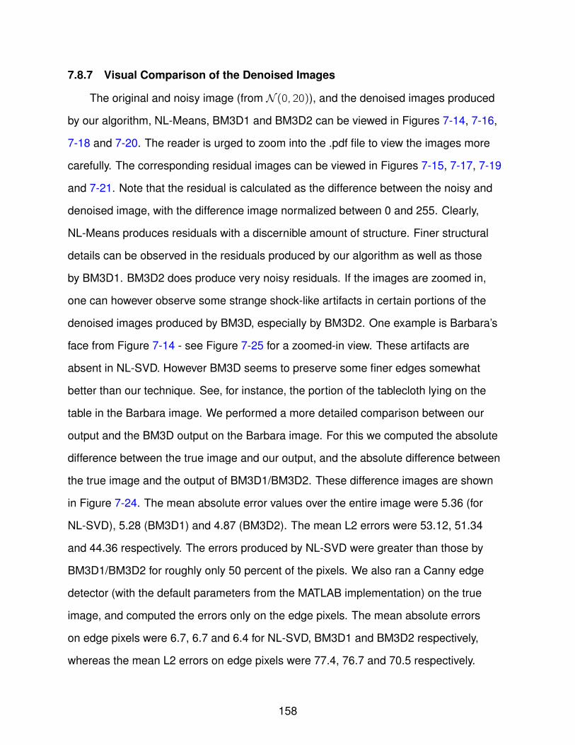
7.8.7 Visual Comparison of the Denoised Images
The original and noisy image (from N (0, 20)), and the denoised images produced
by our algorithm, NL-Means, BM3D1 and BM3D2 can be viewed in Figures 7-14, 7-16,
7-18 and 7-20. The reader is urged to zoom into the .pdf file to view the images more
carefully. The corresponding residual images can be viewed in Figures 7-15, 7-17, 7-19
and 7-21. Note that the residual is calculated as the difference between the noisy and
denoised image, with the difference image normalized between 0 and 255. Clearly,
NL-Means produces residuals with a discernible amount of structure. Finer structural
details can be observed in the residuals produced by our algorithm as well as those
by BM3D1. BM3D2 does produce very noisy residuals. If the images are zoomed in,
one can however observe some strange shock-like artifacts in certain portions of the
denoised images produced by BM3D, especially by BM3D2. One example is Barbara’s
face from Figure 7-14 - see Figure 7-25 for a zoomed-in view. These artifacts are
absent in NL-SVD. However BM3D seems to preserve some finer edges somewhat
better than our technique. See, for instance, the portion of the tablecloth lying on the
table in the Barbara image. We performed a more detailed comparison between our
output and the BM3D output on the Barbara image. For this we computed the absolute
difference between the true image and our output, and the absolute difference between
the true image and the output of BM3D1/BM3D2. These difference images are shown
in Figure 7-24. The mean absolute error values over the entire image were 5.36 (for
NL-SVD), 5.28 (BM3D1) and 4.87 (BM3D2). The mean L2 errors were 53.12, 51.34
and 44.36 respectively. The errors produced by NL-SVD were greater than those by
BM3D1/BM3D2 for roughly only 50 percent of the pixels. We also ran a Canny edge
detector (with the default parameters from the MATLAB implementation) on the true
image, and computed the errors only on the edge pixels. The mean absolute errors
on edge pixels were 6.7, 6.7 and 6.4 for NL-SVD, BM3D1 and BM3D2 respectively,
whereas the mean L2 errors on edge pixels were 77.4, 76.7 and 70.5 respectively.
158
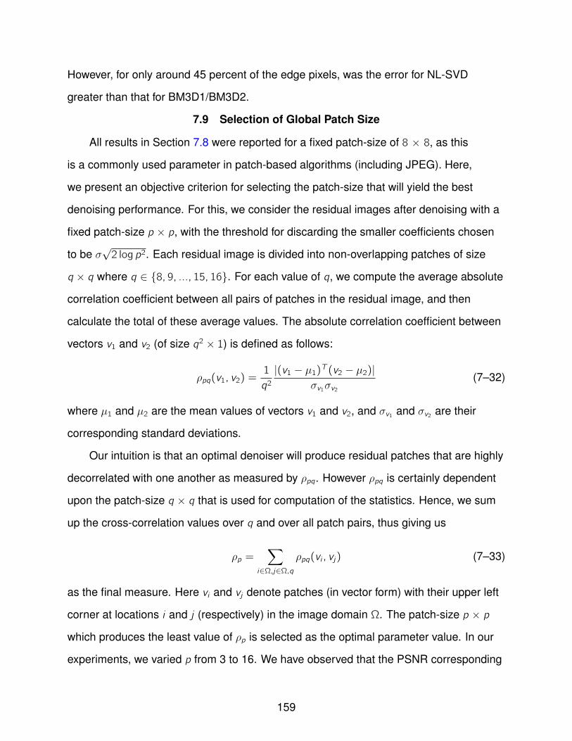
However, for only around 45 percent of the edge pixels, was the error for NL-SVD
greater than that for BM3D1/BM3D2.
7.9 Selection of Global Patch Size
All results in Section 7.8 were reported for a fixed patch-size of 8 × 8, as this
is a commonly used parameter in patch-based algorithms (including JPEG). Here,
we present an objective criterion for selecting the patch-size that will yield the best
denoising performance. For this, we consider the residual images after denoising with a
fixed patch-size p × p, with the threshold for discarding the smaller coefficients chosen
to be σ√2 log p2. Each residual image is divided into non-overlapping patches of size
q × q where q ∈ 8, 9, ..., 15, 16. For each value of q, we compute the average absolute
correlation coefficient between all pairs of patches in the residual image, and then
calculate the total of these average values. The absolute correlation coefficient between
vectors v1 and v2 (of size q2 × 1) is defined as follows:
ρpq(v1, v2) =1
q2|(v1 − µ1)
T (v2 − µ2)|σv1σv2
(7–32)
where µ1 and µ2 are the mean values of vectors v1 and v2, and σv1 and σv2 are their
corresponding standard deviations.
Our intuition is that an optimal denoiser will produce residual patches that are highly
decorrelated with one another as measured by ρpq. However ρpq is certainly dependent
upon the patch-size q × q that is used for computation of the statistics. Hence, we sum
up the cross-correlation values over q and over all patch pairs, thus giving us
ρp =∑
i∈Ω,j∈Ω,q
ρpq(vi , vj) (7–33)
as the final measure. Here vi and vj denote patches (in vector form) with their upper left
corner at locations i and j (respectively) in the image domain Ω. The patch-size p × p
which produces the least value of ρp is selected as the optimal parameter value. In our
experiments, we varied p from 3 to 16. We have observed that the PSNR corresponding
159
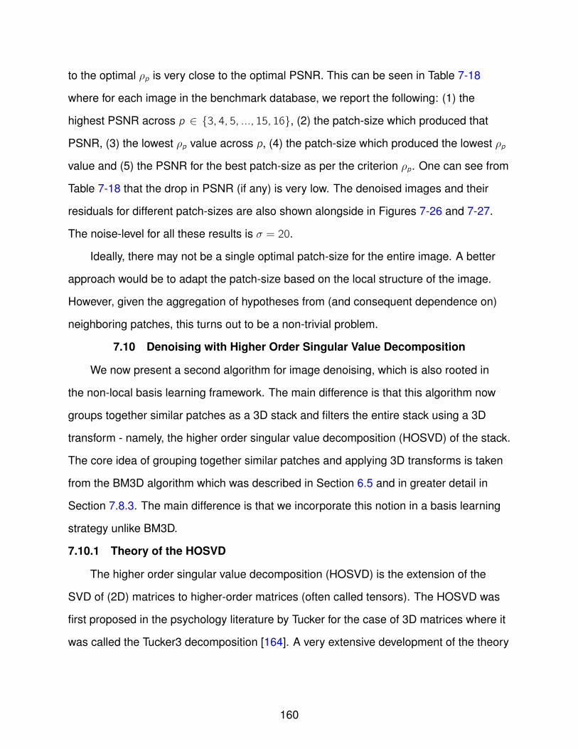
to the optimal ρp is very close to the optimal PSNR. This can be seen in Table 7-18
where for each image in the benchmark database, we report the following: (1) the
highest PSNR across p ∈ 3, 4, 5, ..., 15, 16, (2) the patch-size which produced that
PSNR, (3) the lowest ρp value across p, (4) the patch-size which produced the lowest ρp
value and (5) the PSNR for the best patch-size as per the criterion ρp. One can see from
Table 7-18 that the drop in PSNR (if any) is very low. The denoised images and their
residuals for different patch-sizes are also shown alongside in Figures 7-26 and 7-27.
The noise-level for all these results is σ = 20.
Ideally, there may not be a single optimal patch-size for the entire image. A better
approach would be to adapt the patch-size based on the local structure of the image.
However, given the aggregation of hypotheses from (and consequent dependence on)
neighboring patches, this turns out to be a non-trivial problem.
7.10 Denoising with Higher Order Singular Value Decomposition
We now present a second algorithm for image denoising, which is also rooted in
the non-local basis learning framework. The main difference is that this algorithm now
groups together similar patches as a 3D stack and filters the entire stack using a 3D
transform - namely, the higher order singular value decomposition (HOSVD) of the stack.
The core idea of grouping together similar patches and applying 3D transforms is taken
from the BM3D algorithm which was described in Section 6.5 and in greater detail in
Section 7.8.3. The main difference is that we incorporate this notion in a basis learning
strategy unlike BM3D.
7.10.1 Theory of the HOSVD
The higher order singular value decomposition (HOSVD) is the extension of the
SVD of (2D) matrices to higher-order matrices (often called tensors). The HOSVD was
first proposed in the psychology literature by Tucker for the case of 3D matrices where it
was called the Tucker3 decomposition [164]. A very extensive development of the theory
160
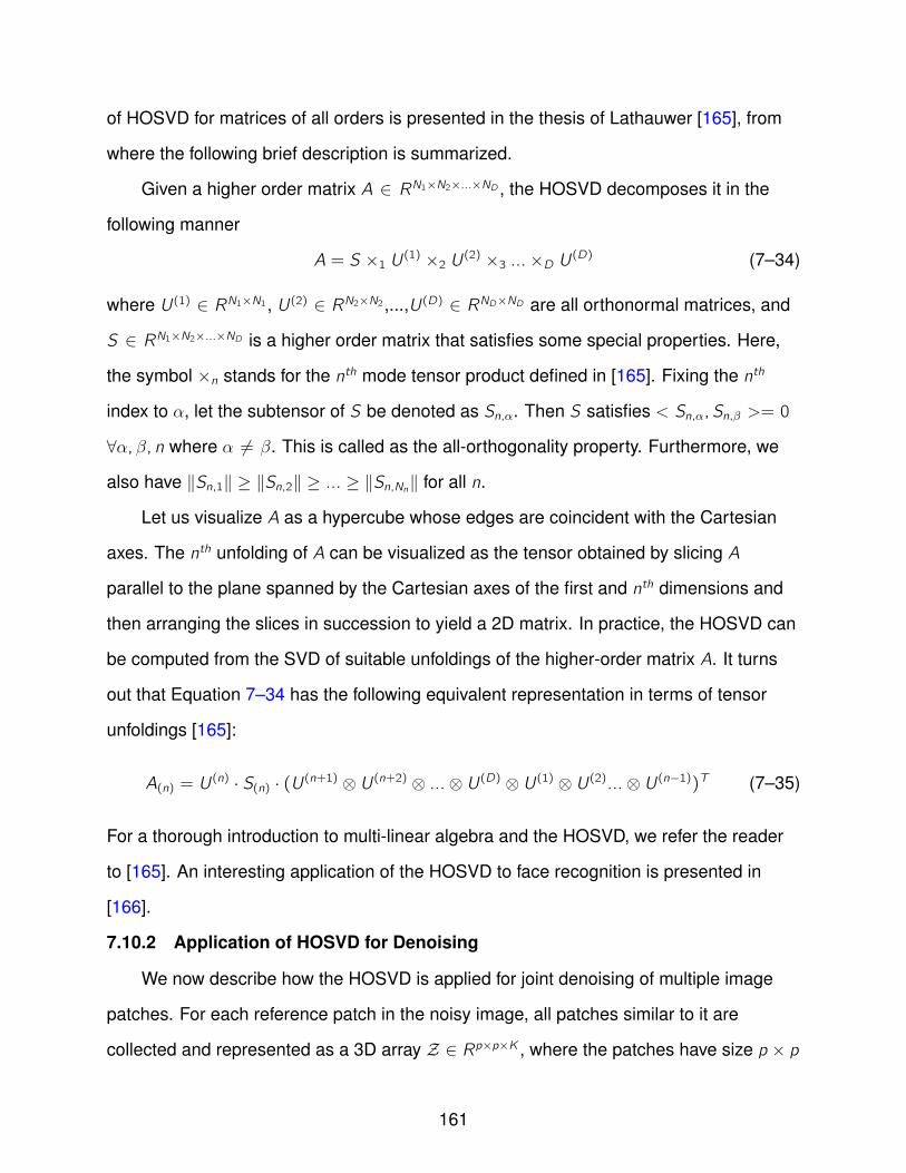
of HOSVD for matrices of all orders is presented in the thesis of Lathauwer [165], from
where the following brief description is summarized.
Given a higher order matrix A ∈ RN1×N2×...×ND , the HOSVD decomposes it in the
following manner
A = S ×1 U(1) ×2 U(2) ×3 ...×D U(D) (7–34)
where U(1) ∈ RN1×N1, U(2) ∈ RN2×N2,...,U(D) ∈ RND×ND are all orthonormal matrices, and
S ∈ RN1×N2×...×ND is a higher order matrix that satisfies some special properties. Here,
the symbol ×n stands for the nth mode tensor product defined in [165]. Fixing the nth
index to α, let the subtensor of S be denoted as Sn,α. Then S satisfies < Sn,α,Sn,β >= 0
∀α, β, n where α 6= β. This is called as the all-orthogonality property. Furthermore, we
also have ‖Sn,1‖ ≥ ‖Sn,2‖ ≥ ... ≥ ‖Sn,Nn‖ for all n.
Let us visualize A as a hypercube whose edges are coincident with the Cartesian
axes. The nth unfolding of A can be visualized as the tensor obtained by slicing A
parallel to the plane spanned by the Cartesian axes of the first and nth dimensions and
then arranging the slices in succession to yield a 2D matrix. In practice, the HOSVD can
be computed from the SVD of suitable unfoldings of the higher-order matrix A. It turns
out that Equation 7–34 has the following equivalent representation in terms of tensor
unfoldings [165]:
A(n) = U(n) · S(n) · (U(n+1) ⊗ U(n+2) ⊗ ...⊗ U(D) ⊗ U(1) ⊗ U(2)...⊗ U(n−1))T (7–35)
For a thorough introduction to multi-linear algebra and the HOSVD, we refer the reader
to [165]. An interesting application of the HOSVD to face recognition is presented in
[166].
7.10.2 Application of HOSVD for Denoising
We now describe how the HOSVD is applied for joint denoising of multiple image
patches. For each reference patch in the noisy image, all patches similar to it are
collected and represented as a 3D array Z ∈ Rp×p×K , where the patches have size p × p
161

and K is the number of similar patches in the ensemble (note that K is spatially varying).
A patch P is said to be similar to the reference patch if ‖P − Pref ‖2 ≤ τ 2d where τd is
defined earlier in Section 7.7.1. The HOSVD of Z is given as follows
Z = S ×1 U(1) ×2 U(2) ×3 U(3) (7–36)
where the orthonormal matrices U(1) ∈ Rp×p, U(2) ∈ Rp×p and U(3) ∈ RK×K can be
computed from the SVD of the unfoldings Z(1), Z(2) and Z(3) respectively. The exact
equations are as follows:
Z(1) = U(1) · S(1) · (U(2) ⊗ U(3))T (7–37)
Z(2) = U(2) · S(2) · (U(3) ⊗ U(1))T (7–38)
Z(3) = U(3) · S(3) · (U(1) ⊗ U(2))T . (7–39)
However, the complexity of the SVD computations for K × K matrices is O(K 3).
To prevent the computations from getting unwieldy, we put an upper cap on the number
of allowed similar patches, i.e. we impose the constraint that K ≤ 30. The patches
from Z are then projected onto the HOSVD transform. The parameter for thresholding
the transform coefficients is picked to be σ√2 log p2K , again as per the rule from [113].
The stack Z is then reconstructed after inverting the transform thereby filtering all
the individual patches. Note that unlike NL-SVD (see Section 7.7.3), we filter all the
individual patches in the ensemble and not just the reference patch. This afforded
additional smoothing on all the patches which was required due to the upper limit of
K ≤ 30 unlike the case with NL-SVD. Again, the reference patch is moved in a sliding
window fashion and the hypotheses appearing at each pixel are averaged to produce
the final filtered image.
7.10.3 Outline of HOSVD Algorithm
The HOSVD for denoising is outlined here below:
1. Divide the image into overlapping patches of size p × p.
162
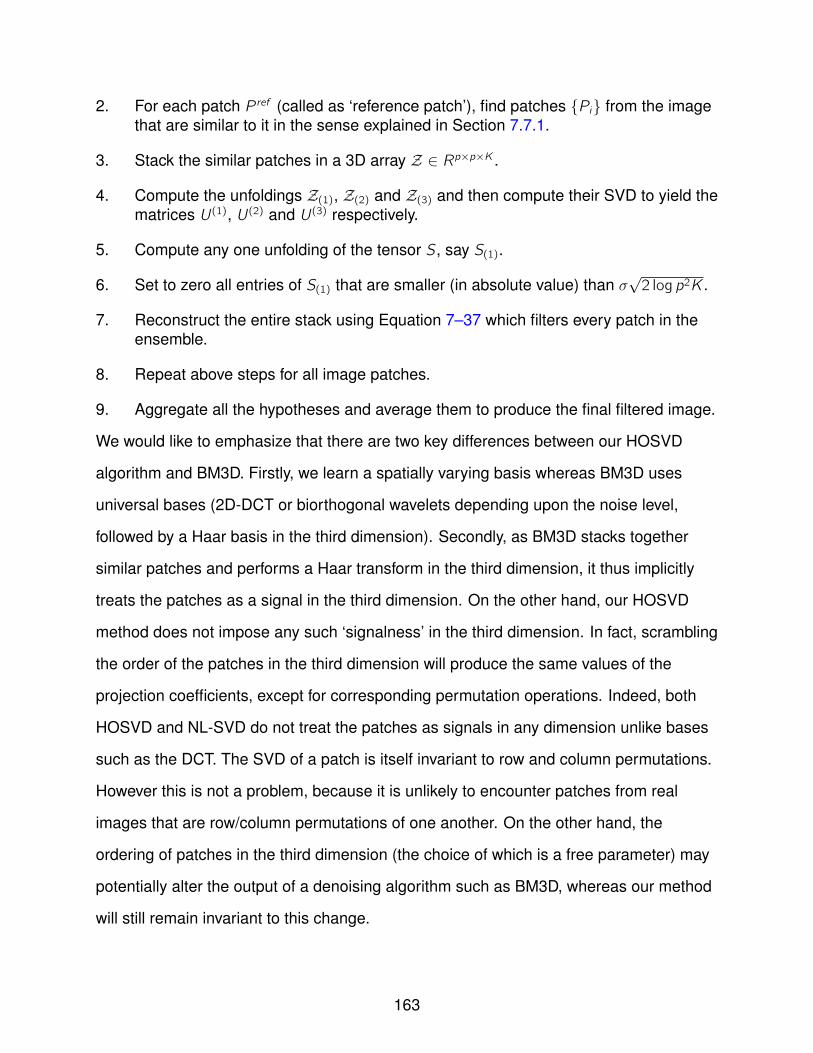
2. For each patch P ref (called as ‘reference patch’), find patches Pi from the imagethat are similar to it in the sense explained in Section 7.7.1.
3. Stack the similar patches in a 3D array Z ∈ Rp×p×K .
4. Compute the unfoldings Z(1), Z(2) and Z(3) and then compute their SVD to yield thematrices U(1), U(2) and U(3) respectively.
5. Compute any one unfolding of the tensor S , say S(1).
6. Set to zero all entries of S(1) that are smaller (in absolute value) than σ√2 log p2K .
7. Reconstruct the entire stack using Equation 7–37 which filters every patch in theensemble.
8. Repeat above steps for all image patches.
9. Aggregate all the hypotheses and average them to produce the final filtered image.
We would like to emphasize that there are two key differences between our HOSVD
algorithm and BM3D. Firstly, we learn a spatially varying basis whereas BM3D uses
universal bases (2D-DCT or biorthogonal wavelets depending upon the noise level,
followed by a Haar basis in the third dimension). Secondly, as BM3D stacks together
similar patches and performs a Haar transform in the third dimension, it thus implicitly
treats the patches as a signal in the third dimension. On the other hand, our HOSVD
method does not impose any such ‘signalness’ in the third dimension. In fact, scrambling
the order of the patches in the third dimension will produce the same values of the
projection coefficients, except for corresponding permutation operations. Indeed, both
HOSVD and NL-SVD do not treat the patches as signals in any dimension unlike bases
such as the DCT. The SVD of a patch is itself invariant to row and column permutations.
However this is not a problem, because it is unlikely to encounter patches from real
images that are row/column permutations of one another. On the other hand, the
ordering of patches in the third dimension (the choice of which is a free parameter) may
potentially alter the output of a denoising algorithm such as BM3D, whereas our method
will still remain invariant to this change.
163

7.11 Experimental Results with HOSVD
The PSNR results for HOSVD are presented in Tables 7.12, 7.12, 7-7, 7-9, 7-12,
7-14 and 7-16. The corresponding SSIM results can be found in Tables 7-4, 7-6,
7-8, 7-10, 7-13, 7-15 and 7-17. From these tables, it can be observed that HOSVD
is superior to KSVD, NL-Means, 3D-DCT and NL-SVD. Indeed, it is also superior to
BM3D1 at higher noise levels (σ ≥ 20) on most images in terms of PSNR/SSIM values,
though it lags slightly behind BM3D2. The average difference between the PSNR values
produced by HOSVD and BM3D2 at noise levels 10, 20 and 30 is 0.346, 0.281 and
0.343 respectively (see Tables 7.12, 7-9 and 7-14).
A comparison between NL-SVD and HOSVD reveals that the latter outperforms
the former on the weaker or finer edges or textures. We have observed that the images
denoised by HOSVD sometimes tend to have a faint grainy appearance. The reason
for this is that HOSVD smoothes an ensemble of patches by projection onto a common
basis followed by truncation of transform coefficients. We have observed experimentally
that this tends to slightly under-smooth the patches, when compared to patches that
are smoothed individually as in techniques like NL-SVD. The undermsoothing is
compensated for by the averaging operations and the filtering of all patches from the
stack. The faint grainy appearance can be mitigated by running a linear smoothing
filter, such as a PCA in the third dimension from patch stacks from the filtered output
of HOSVD (similar to the Wiener filter idea implemented in BM3D2 but with a learning
component involving PCA on the stack of corresponding pixels from similar patches),
which seems to improve subjective visual quality (in our opinion). We leave a rigorous
testing of this issue for future work.
7.12 Comparison of Time Complexity
We now present a time complexity analysis of all the competing algorithms. For
this, assume that the number of image pixels is N and the average time to compute
similar patches per reference patch is TS . Let us assume that the average number of
164
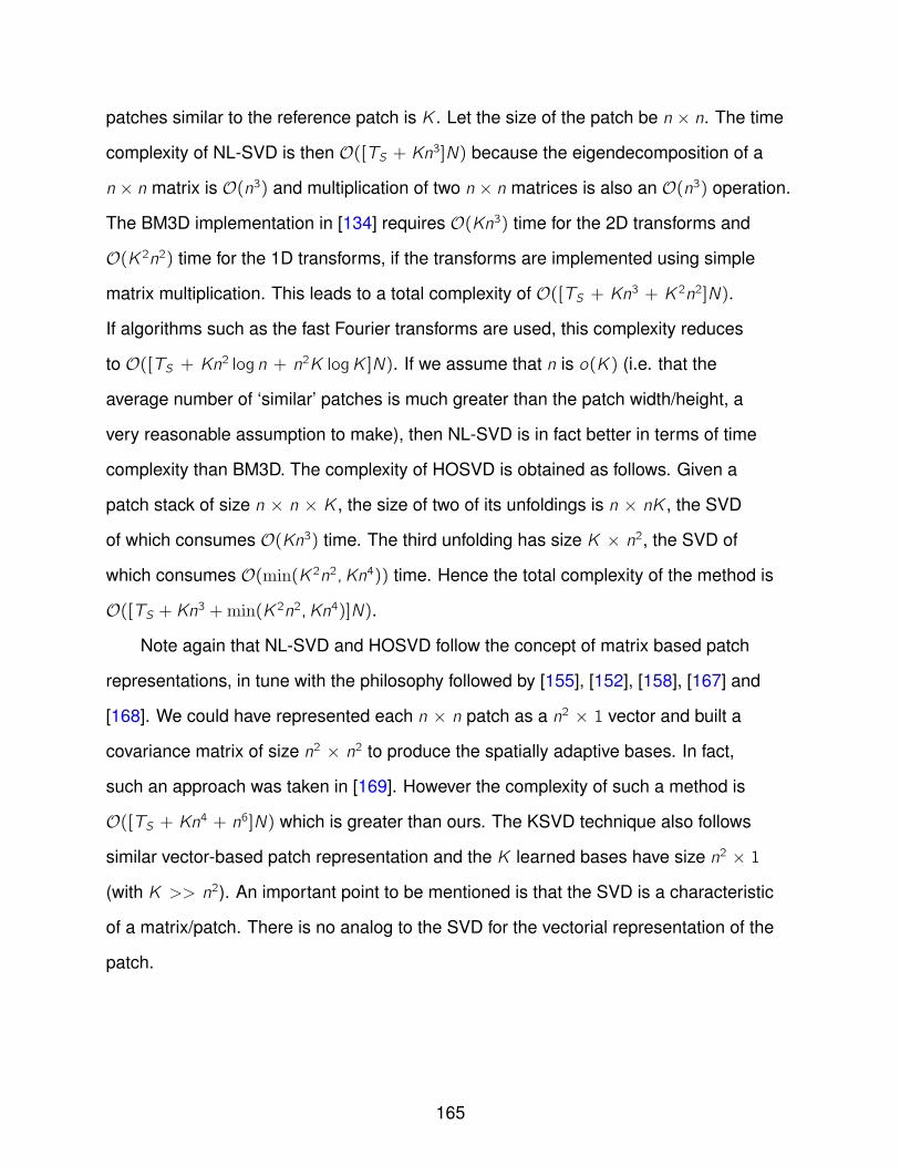
patches similar to the reference patch is K . Let the size of the patch be n × n. The time
complexity of NL-SVD is then O([TS + Kn3]N) because the eigendecomposition of a
n × n matrix is O(n3) and multiplication of two n × n matrices is also an O(n3) operation.
The BM3D implementation in [134] requires O(Kn3) time for the 2D transforms and
O(K 2n2) time for the 1D transforms, if the transforms are implemented using simple
matrix multiplication. This leads to a total complexity of O([TS + Kn3 + K 2n2]N).
If algorithms such as the fast Fourier transforms are used, this complexity reduces
to O([TS + Kn2 log n + n2K logK ]N). If we assume that n is o(K) (i.e. that the
average number of ‘similar’ patches is much greater than the patch width/height, a
very reasonable assumption to make), then NL-SVD is in fact better in terms of time
complexity than BM3D. The complexity of HOSVD is obtained as follows. Given a
patch stack of size n × n × K , the size of two of its unfoldings is n × nK , the SVD
of which consumes O(Kn3) time. The third unfolding has size K × n2, the SVD of
which consumes O(min(K 2n2,Kn4)) time. Hence the total complexity of the method is
O([TS + Kn3 +min(K 2n2,Kn4)]N).
Note again that NL-SVD and HOSVD follow the concept of matrix based patch
representations, in tune with the philosophy followed by [155], [152], [158], [167] and
[168]. We could have represented each n × n patch as a n2 × 1 vector and built a
covariance matrix of size n2 × n2 to produce the spatially adaptive bases. In fact,
such an approach was taken in [169]. However the complexity of such a method is
O([TS + Kn4 + n6]N) which is greater than ours. The KSVD technique also follows
similar vector-based patch representation and the K learned bases have size n2 × 1
(with K >> n2). An important point to be mentioned is that the SVD is a characteristic
of a matrix/patch. There is no analog to the SVD for the vectorial representation of the
patch.
165
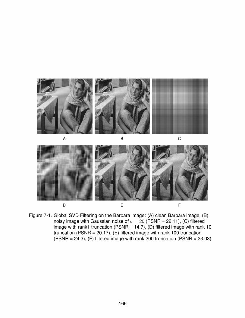
A B C
D E F
Figure 7-1. Global SVD Filtering on the Barbara image: (A) clean Barbara image, (B)noisy image with Gaussian noise of σ = 20 (PSNR = 22.11), (C) filteredimage with rank1 truncation (PSNR = 14.7), (D) filtered image with rank 10truncation (PSNR = 20.17), (E) filtered image with rank 100 truncation(PSNR = 24.3), (F) filtered image with rank 200 truncation (PSNR = 23.03)
166
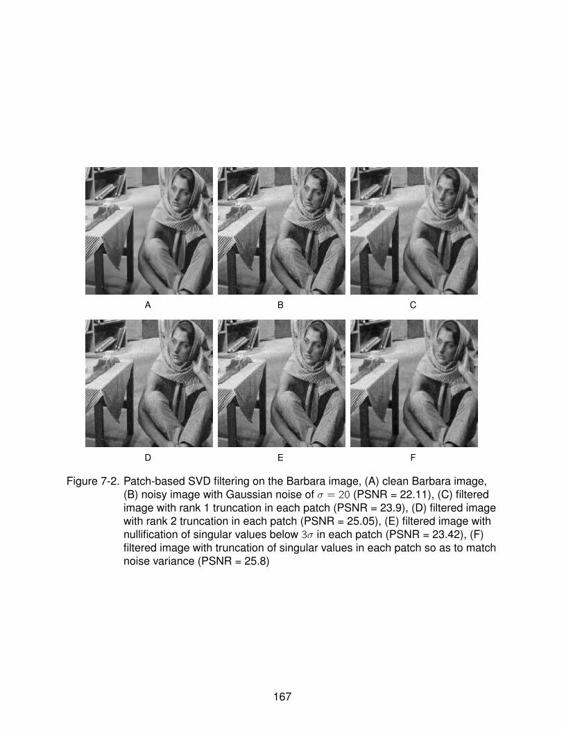
A B C
D E F
Figure 7-2. Patch-based SVD filtering on the Barbara image, (A) clean Barbara image,(B) noisy image with Gaussian noise of σ = 20 (PSNR = 22.11), (C) filteredimage with rank 1 truncation in each patch (PSNR = 23.9), (D) filtered imagewith rank 2 truncation in each patch (PSNR = 25.05), (E) filtered image withnullification of singular values below 3σ in each patch (PSNR = 23.42), (F)filtered image with truncation of singular values in each patch so as to matchnoise variance (PSNR = 25.8)
167

A B C
D E
Figure 7-3. Oracle filter with SVD, (A) clean Barbara image, (B) noisy image withGaussian noise of σ = 20 (PSNR = 22.11), (C) filtered image withnullification of all the values in the projection matrix below 3σ in each patch(PSNR = 36.9), (D) noisy image with Gaussian noise of σ = 40 (PSNR =22.11), (E) filtered image with nullification of all the values in the projectionmatrix below 3σ in each patch (PSNR = 31.34)
Figure 7-4. Fifteen synthetic patches
168
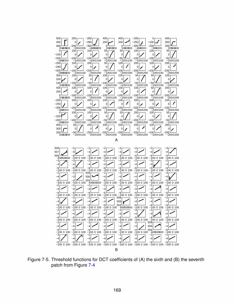
200400600400450500
−2000200−200
0200
−400−300−200−300−280−260
1002003000
200400
1002003000
200400
−400−2000−300−250−200
−200−1000−200−100
0
200300400200300400
−200−1000−200−100
0
−1000100−100
0100
−1000100−100
0100
−1000100−50
050
−1000100−50
050
−1000100−100
0100
−1000100−100
0100
−1000100−50
050
−400−300−200−300−280−260
−1000100−100
0100
−2000200−200
0200
−1000100−50
050
−2000200−100
0100
−2000200−200
0200
−1000100−100
0100
−2000200−200
0200
100200300100200300
−1000100−100
0100
−1000100−50
050
−1000100−100
0100
−1000100−100
0100
−1000100−50
050
−1000100−50
050
−1000100−100
0100
1002003000
200400
−1000100−100
0100
−2000200−100
0100
−1000100−100
0100
−1000100−100
0100
−1000100−100
0100
−1000100−50
050
−2000200−200
0200
−400−2000−300−250−200
−1000100−100
0100
−2000200−200
0200
−1000100−100
0100
−2000200−100
0100
−2000200−200
0200
−2000200−200
0200
−2000200−100
0100
−200−1000−400−200
0
−1000100−100
0100
−1000100−100
0100
−1000100−50
050
−1000100−50
050
−2000200−200
0200
−1000100−100
0100
−1000100−50
050
200300400200300400
−1000100−50
050
−2000200−200
0200
−2000200−200
0200
−2000200−200
0200
−2000200−200
0200
−1000100−100
0100
−2000200−200
0200
A
400500600506507508
−100 0 100−6−4−2
−100 0 100−6−4−2
−100 0 100−6−4−2
−100 0 100−6−4−2
−100 0 100−6−4−2
−100 0 100−6−4−2
−100 0 100−5−4−3
−100 0 100−5−4−3
−100 0 100−5−4−3
−100 0 100−6−4−2
−100 0 100−6−4−2
−100 0 100−6−4−2
−100 0 100−6−4−2
−100 0 100−5−4−3
−100 0 100−6−4−2
−100 0 100−6−4−2
−100 0 100−4−3−2
400500600504506508
−100 0 100−6−4−2
−100 0 100−6−4−2
−100 0 100−6−4−2
−100 0 100−6−4−2
−100 0 100−5−4−3
−100 0 100−6−4−2
−100 0 100−6−4−2
−100 0 100−6−4−2
−100 0 100−6−4−2
−100 0 100−6−4−2
−100 0 100−6−4−2
−100 0 100−6−4−2
−100 0 100−6−4−2
−100 0 100−5−4−3
−100 0 100−6−4−2
−100 0 100−6−4−2
−100 0 100−6−4−2
400500600504506508
−100 0 100−6−4−2
−100 0 100−6−4−2
−100 0 100−6−4−2
−100 0 100−6−4−2
−100 0 100−6−4−2
−100 0 100−6−4−2
−100 0 100−6−4−2
−100 0 100−6−4−2
−100 0 100−5−4−3
−100 0 100−6−4−2
−100 0 100−6−4−2
−100 0 100−6−4−2
−100 0 100−6−4−2
−100 0 100−6−4−2
−100 0 100−6−4−2
−100 0 100−6−4−2
−100 0 100−4−3−2
400500600504506508
−100 0 100−6−4−2
−100 0 100−5−4−3
−100 0 100−5−4−3
−100 0 100−6−4−2
−100 0 100−6−4−2
−100 0 100−6−4−2
−100 0 100−6−4−2
−100 0 100−6−4−2
−100 0 100−6−4−2
B
Figure 7-5. Threshold functions for DCT coefficients of (A) the sixth and (B) the seventhpatch from Figure 7-4
169
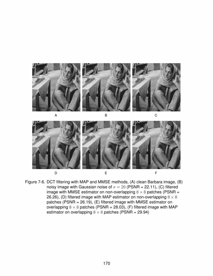
A B C
D E F
Figure 7-6. DCT filtering with MAP and MMSE methods, (A) clean Barbara image, (B)noisy image with Gaussian noise of σ = 20 (PSNR = 22.11), (C) filteredimage with MMSE estimator on non-overlapping 8× 8 patches (PSNR =26.26), (D) filtered image with MAP estimator on non-overlapping 8× 8patches (PSNR = 26.19), (E) filtered image with MMSE estimator onoverlapping 8× 8 patches (PSNR = 28.03), (F) filtered image with MAPestimator on overlapping 8× 8 patches (PSNR = 29.94)
170

A B C
D E F
Figure 7-7. DCT filtering with MAP and MMSE methods, (A) clean Barbara image, (B)noisy image with Gaussian noise of σ = 20 (PSNR = 22.11), (C) filteredimage with MMSE estimator on non-overlapping 8× 8 patches (PSNR =27.12), (D) filtered image with MAP estimator on non-overlapping 8× 8patches (PSNR = 26.9), (E) filtered image with MMSE estimator onoverlapping 8× 8 patches (PSNR = 29.1), (F) filtered image with MAPestimator on overlapping 8× 8 patches (PSNR = 29.94)
171
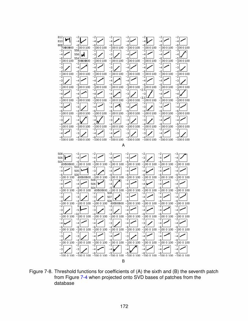
700800900808810812
−100 0 100−6−4−2
−100 0 100−6−4−2
−100 0 100−6−4−2
−100 0 100−6−4−2
−100 0 100−6−4−2
−100 0 100−6−4−2
−100 0 100−6−4−2
−100 0 100−6−4−2
400600800554556558
−100 0 100−4−3−2
−100 0 100−4−3−2
−100 0 100−6−4−2
−100 0 100−6−4−2
−100 0 100−6−4−2
−100 0 100−5−4−3
−100 0 100−4−3−2
−100 0 100−6−4−2
−100 0 100−6−4−2
−100 0 100−4−3−2
−100 0 100−6−4−2
−100 0 100−6−4−2
−100 0 100−6−4−2
−100 0 100−4−3−2
−100 0 100−4−3−2
−100 0 100−6−4−2
−100 0 100−6−4−2
−100 0 100−6−4−2
−100 0 100−6−4−2
−100 0 100−6−4−2
−100 0 100−6−4−2
−100 0 100−4−3−2
−100 0 100−6−4−2
−100 0 100−6−4−2
−100 0 100−6−4−2
−100 0 100−6−4−2
−100 0 100−4−3−2
−100 0 100−3.5
−3−2.5
−100 0 100−6−4−2
−100 0 100−5−4−3
−100 0 100−6−4−2
−100 0 100−4−3−2
−100 0 100−6−4−2
−100 0 100−6−4−2
−100 0 100−6−4−2
−100 0 100−4−3−2
−100 0 100−6−4−2
−100 0 100−6−4−2
−100 0 100−4−3−2
−100 0 100−5−4−3
−100 0 100−5−4−3
−100 0 100−4−3−2
−100 0 100−4−3−2
−100 0 100−4−3−2
−100 0 100−6−4−2
−100 0 100−6−4−2
−100 0 100−6−4−2
−100 0 100−4−3−2
−100 0 100−6−4−2
−100 0 100−6−4−2
−100 0 100−4−3−2
−100 0 100−4−3−2
−100 0 100−6−4−2
−100 0 100−4−3−2
A
400500600504506508
−100 0 100−6−4−2
−100 0 100−6−4−2
−100 0 100−6−4−2
−100 0 100−6−4−2
−100 0 100−4−3−2
−100 0 100−6−4−2
−100 0 100−5−4−3
−100 0 100−6−4−2
400500600500505510
−100 0 100−4−3−2
−100 0 100−6−4−2
−100 0 100−6−4−2
−100 0 100−6−4−2
−100 0 100−6−4−2
−100 0 100−6−4−2
−100 0 100−6−4−2
−100 0 100−6−4−2
400500600504506508
−100 0 100−5−4−3
−100 0 100−6−4−2
−100 0 100−6−4−2
−100 0 100−6−4−2
−100 0 100−6−4−2
−100 0 100−4−3−2
−100 0 100−4−3−2
−100 0 100−4−3−2
400500600506507508
−100 0 100−6−4−2
−100 0 100−6−4−2
−100 0 100−6−4−2
−100 0 100−6−4−2
−100 0 100−4−3−2
−100 0 100−10
−50
−100 0 100−4−3−2
−100 0 100−4−3−2
−100 0 100−6−4−2
−100 0 100−6−4−2
−100 0 100−6−4−2
−100 0 100−6−4−2
−100 0 100−6−4−2
−100 0 100−6−4−2
−100 0 100−6−4−2
−100 0 100−4−3−2
−100 0 100−6−4−2
−100 0 100−4−3−2
−100 0 100−6−4−2
−100 0 100−6−4−2
−100 0 100−4−3−2
−100 0 100−4−3−2
−100 0 100−6−4−2
−100 0 100−6−4−2
−100 0 100−4−3−2
−100 0 100−6−4−2
−100 0 100−6−4−2
−100 0 100−6−4−2
−100 0 100−4−3−2
−100 0 100−4−3−2
−100 0 100−6−4−2
−100 0 100−5−4−3
−100 0 100−5−4−3
−100 0 100−6−4−2
−100 0 100−6−4−2
−100 0 100−6−4−2
B
Figure 7-8. Threshold functions for coefficients of (A) the sixth and (B) the seventh patchfrom Figure 7-4 when projected onto SVD bases of patches from thedatabase
172
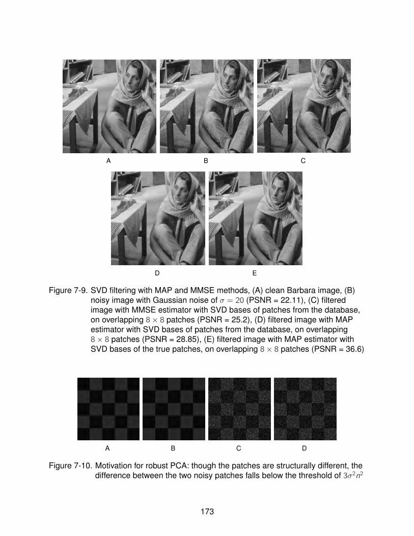
A B C
D E
Figure 7-9. SVD filtering with MAP and MMSE methods, (A) clean Barbara image, (B)noisy image with Gaussian noise of σ = 20 (PSNR = 22.11), (C) filteredimage with MMSE estimator with SVD bases of patches from the database,on overlapping 8× 8 patches (PSNR = 25.2), (D) filtered image with MAPestimator with SVD bases of patches from the database, on overlapping8× 8 patches (PSNR = 28.85), (E) filtered image with MAP estimator withSVD bases of the true patches, on overlapping 8× 8 patches (PSNR = 36.6)
A B C D
Figure 7-10. Motivation for robust PCA: though the patches are structurally different, thedifference between the two noisy patches falls below the threshold of 3σ2n2
173

A B
C
Figure 7-11. Barbara image, (A) reference patch, (B) patches similar to the referencepatch (similarity measured on noisy image which is not shown here), (C)correlation matrices (top row) and learned bases
174
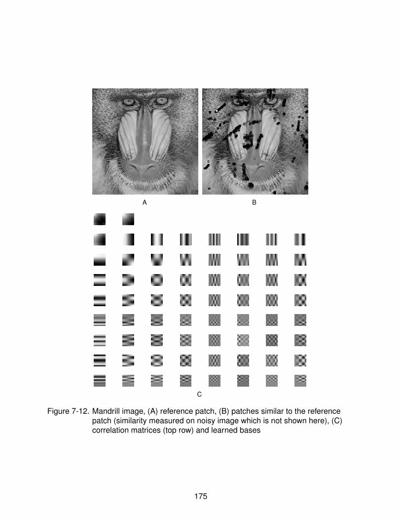
A B
C
Figure 7-12. Mandrill image, (A) reference patch, (B) patches similar to the referencepatch (similarity measured on noisy image which is not shown here), (C)correlation matrices (top row) and learned bases
175

Figure 7-13. DCT bases (8× 8).
176
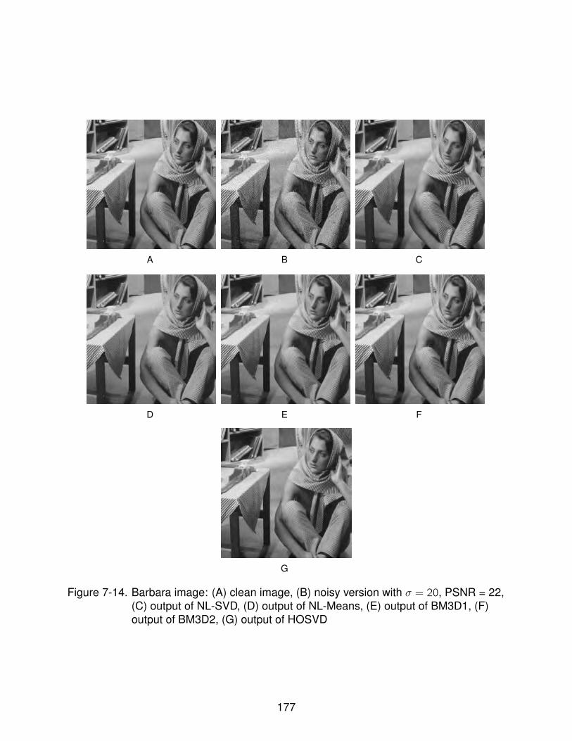
A B C
D E F
G
Figure 7-14. Barbara image: (A) clean image, (B) noisy version with σ = 20, PSNR = 22,(C) output of NL-SVD, (D) output of NL-Means, (E) output of BM3D1, (F)output of BM3D2, (G) output of HOSVD
177
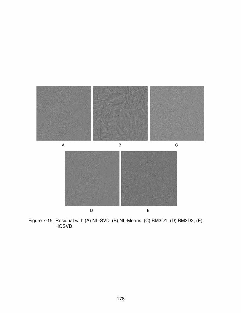
A B C
D E
Figure 7-15. Residual with (A) NL-SVD, (B) NL-Means, (C) BM3D1, (D) BM3D2, (E)HOSVD
178

A B C
D E F
G
Figure 7-16. Boat image: (A) clean image, (B) noisy version with σ = 20, PSNR = 22,(C) output of NL-SVD, (D) output of NL-Means, (E) output of BM3D1, (F)output of BM3D2, (G) output of HOSVD
179
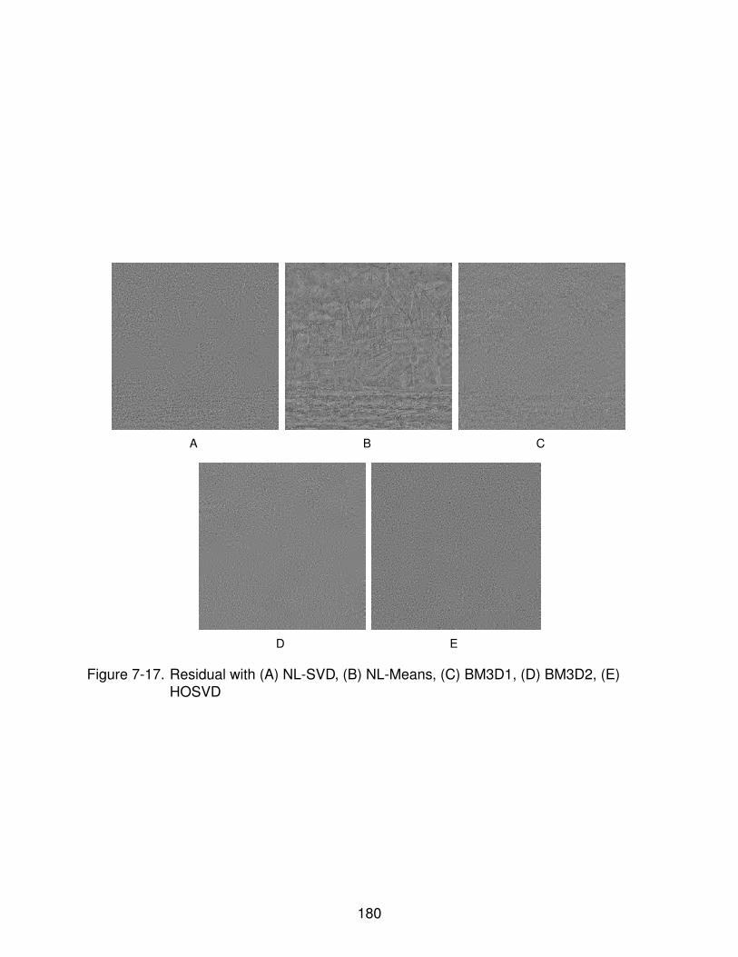
A B C
D E
Figure 7-17. Residual with (A) NL-SVD, (B) NL-Means, (C) BM3D1, (D) BM3D2, (E)HOSVD
180

A B C
D E F
G
Figure 7-18. Stream image: (A) clean image, (B) noisy version with σ = 20, PSNR = 22,(C) output of NL-SVD, (D) output of NL-Means, (E) output of BM3D1, (F)output of BM3D2, (G) output of HOSVD
181
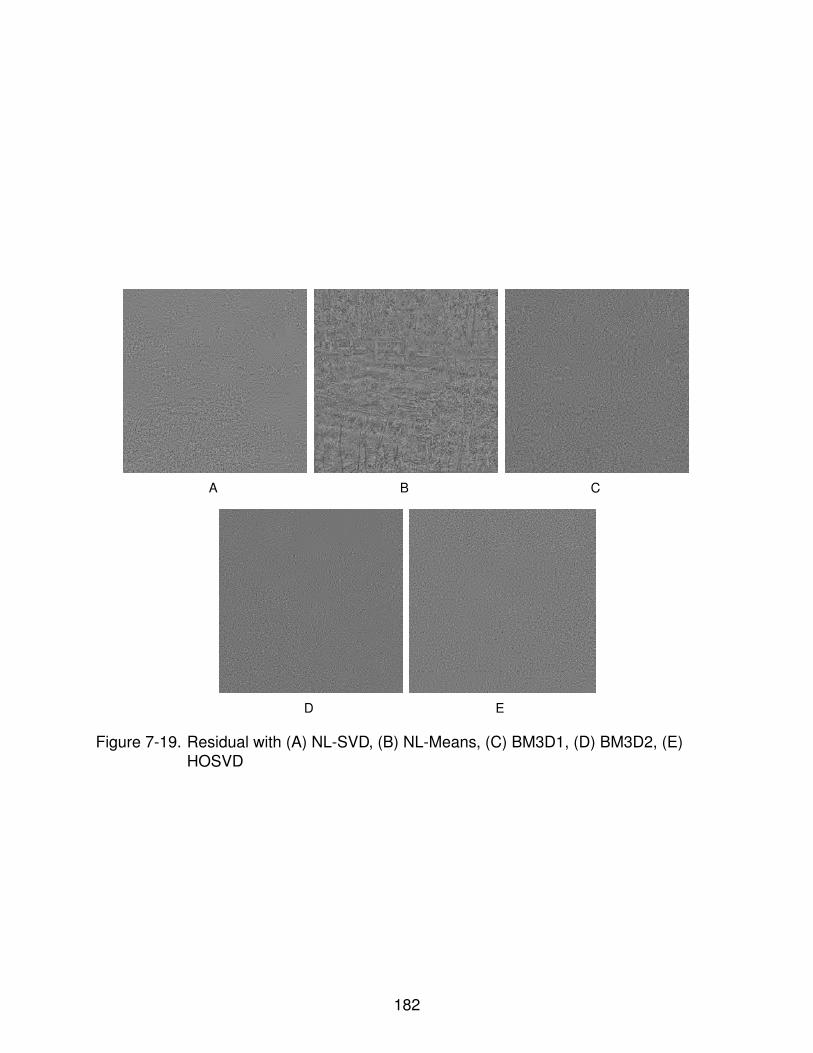
A B C
D E
Figure 7-19. Residual with (A) NL-SVD, (B) NL-Means, (C) BM3D1, (D) BM3D2, (E)HOSVD
182
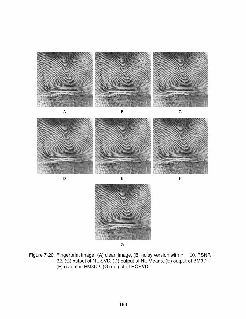
A B C
D E F
G
Figure 7-20. Fingerprint image: (A) clean image, (B) noisy version with σ = 20, PSNR =22, (C) output of NL-SVD, (D) output of NL-Means, (E) output of BM3D1,(F) output of BM3D2, (G) output of HOSVD
183
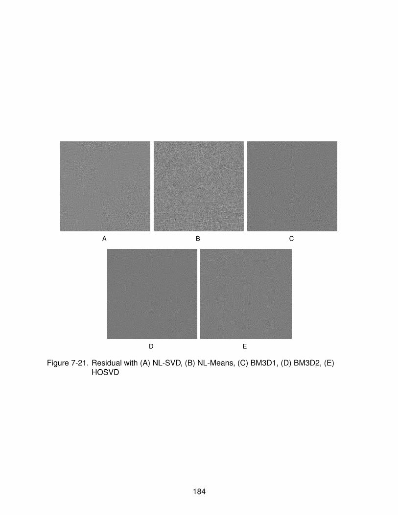
A B C
D E
Figure 7-21. Residual with (A) NL-SVD, (B) NL-Means, (C) BM3D1, (D) BM3D2, (E)HOSVD
184
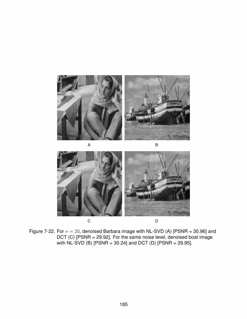
A B
C D
Figure 7-22. For σ = 20, denoised Barbara image with NL-SVD (A) [PSNR = 30.96] andDCT (C) [PSNR = 29.92]. For the same noise level, denoised boat imagewith NL-SVD (B) [PSNR = 30.24] and DCT (D) [PSNR = 29.95].
185
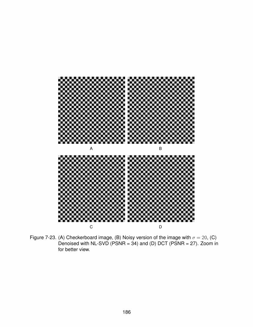
A B
C D
Figure 7-23. (A) Checkerboard image, (B) Noisy version of the image with σ = 20, (C)Denoised with NL-SVD (PSNR = 34) and (D) DCT (PSNR = 27). Zoom infor better view.
186
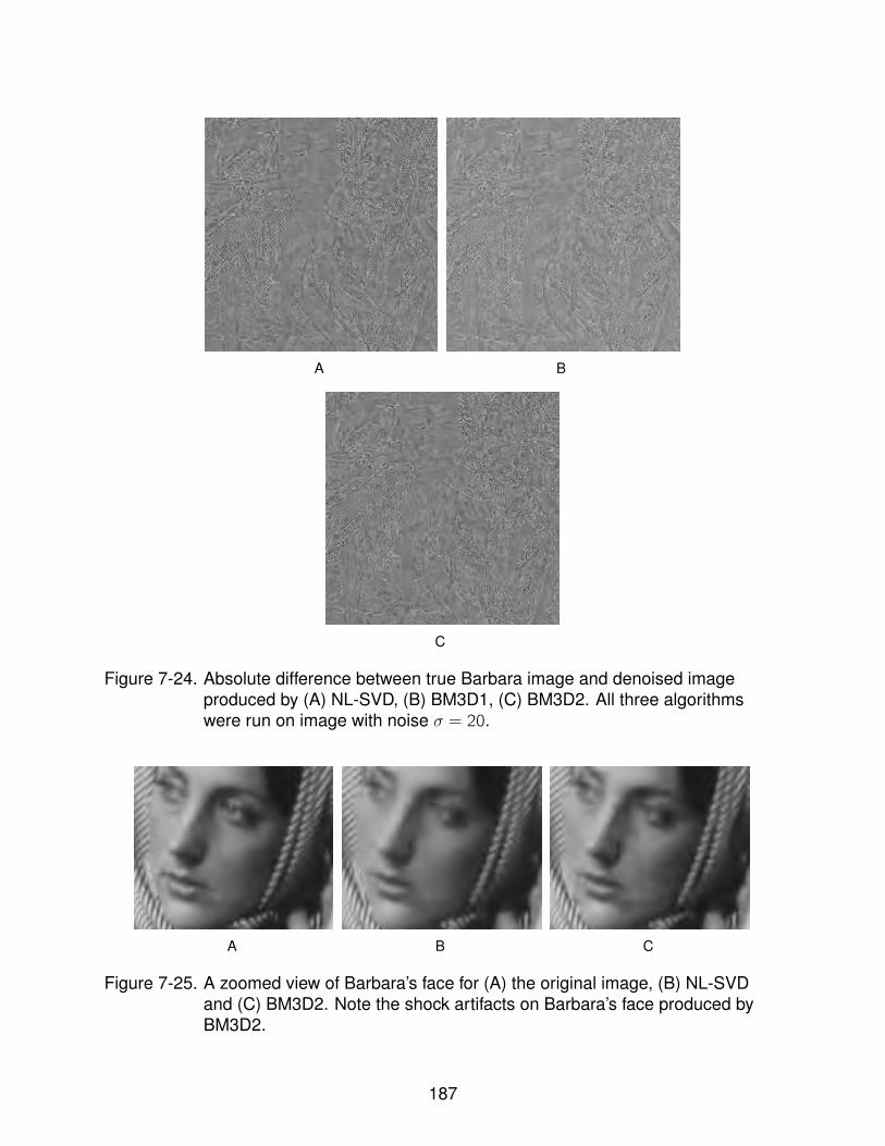
A B
C
Figure 7-24. Absolute difference between true Barbara image and denoised imageproduced by (A) NL-SVD, (B) BM3D1, (C) BM3D2. All three algorithmswere run on image with noise σ = 20.
A B C
Figure 7-25. A zoomed view of Barbara’s face for (A) the original image, (B) NL-SVDand (C) BM3D2. Note the shock artifacts on Barbara’s face produced byBM3D2.
187
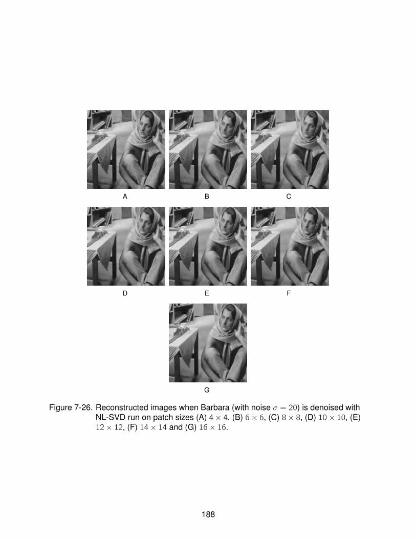
A B C
D E F
G
Figure 7-26. Reconstructed images when Barbara (with noise σ = 20) is denoised withNL-SVD run on patch sizes (A) 4× 4, (B) 6× 6, (C) 8× 8, (D) 10× 10, (E)12× 12, (F) 14× 14 and (G) 16× 16.
188
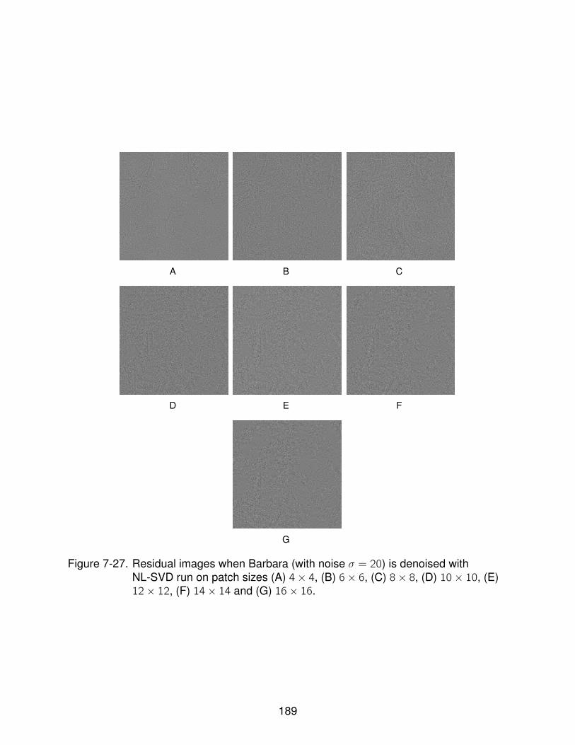
A B C
D E F
G
Figure 7-27. Residual images when Barbara (with noise σ = 20) is denoised withNL-SVD run on patch sizes (A) 4× 4, (B) 6× 6, (C) 8× 8, (D) 10× 10, (E)12× 12, (F) 14× 14 and (G) 16× 16.
189
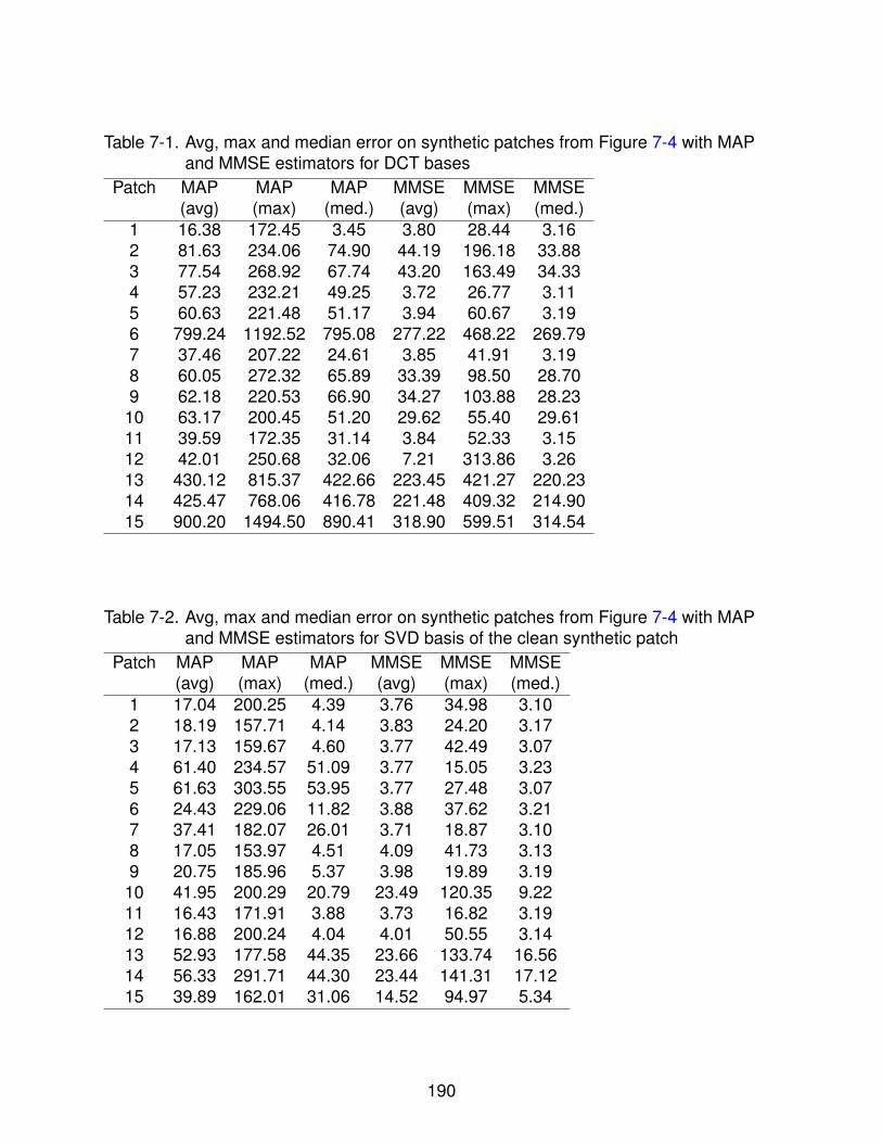
Table 7-1. Avg, max and median error on synthetic patches from Figure 7-4 with MAPand MMSE estimators for DCT bases
Patch MAP MAP MAP MMSE MMSE MMSE(avg) (max) (med.) (avg) (max) (med.)
1 16.38 172.45 3.45 3.80 28.44 3.162 81.63 234.06 74.90 44.19 196.18 33.883 77.54 268.92 67.74 43.20 163.49 34.334 57.23 232.21 49.25 3.72 26.77 3.115 60.63 221.48 51.17 3.94 60.67 3.196 799.24 1192.52 795.08 277.22 468.22 269.797 37.46 207.22 24.61 3.85 41.91 3.198 60.05 272.32 65.89 33.39 98.50 28.709 62.18 220.53 66.90 34.27 103.88 28.2310 63.17 200.45 51.20 29.62 55.40 29.6111 39.59 172.35 31.14 3.84 52.33 3.1512 42.01 250.68 32.06 7.21 313.86 3.2613 430.12 815.37 422.66 223.45 421.27 220.2314 425.47 768.06 416.78 221.48 409.32 214.9015 900.20 1494.50 890.41 318.90 599.51 314.54
Table 7-2. Avg, max and median error on synthetic patches from Figure 7-4 with MAPand MMSE estimators for SVD basis of the clean synthetic patch
Patch MAP MAP MAP MMSE MMSE MMSE(avg) (max) (med.) (avg) (max) (med.)
1 17.04 200.25 4.39 3.76 34.98 3.102 18.19 157.71 4.14 3.83 24.20 3.173 17.13 159.67 4.60 3.77 42.49 3.074 61.40 234.57 51.09 3.77 15.05 3.235 61.63 303.55 53.95 3.77 27.48 3.076 24.43 229.06 11.82 3.88 37.62 3.217 37.41 182.07 26.01 3.71 18.87 3.108 17.05 153.97 4.51 4.09 41.73 3.139 20.75 185.96 5.37 3.98 19.89 3.1910 41.95 200.29 20.79 23.49 120.35 9.2211 16.43 171.91 3.88 3.73 16.82 3.1912 16.88 200.24 4.04 4.01 50.55 3.1413 52.93 177.58 44.35 23.66 133.74 16.5614 56.33 291.71 44.30 23.44 141.31 17.1215 39.89 162.01 31.06 14.52 94.97 5.34
190
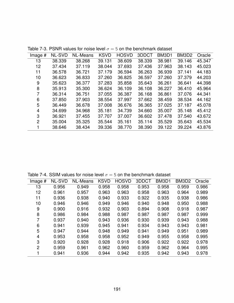
Table 7-3. PSNR values for noise level σ = 5 on the benchmark datasetImage # NL-SVD NL-Means KSVD HOSVD 3DDCT BM3D1 BM3D2 Oracle
13 38.339 38.268 39.131 38.609 38.339 38.981 39.146 45.34712 37.434 37.119 38.044 37.693 37.436 37.963 38.143 45.02311 36.578 36.721 37.179 36.594 36.263 36.939 37.141 44.18310 36.623 36.833 37.260 36.825 36.597 37.260 37.379 44.2039 35.623 36.377 37.283 35.858 35.643 36.261 36.641 44.3988 35.913 35.300 36.624 36.109 36.108 36.227 36.410 45.9647 36.314 36.751 37.055 36.387 36.168 36.861 37.076 44.3416 37.850 37.903 38.554 37.997 37.662 38.459 38.534 44.1625 36.449 36.678 37.008 36.676 36.365 37.025 37.187 45.0784 34.699 34.968 35.181 34.739 34.660 35.007 35.148 45.4123 36.921 37.455 37.707 37.007 36.602 37.478 37.540 43.6722 35.004 35.325 35.544 35.161 35.114 35.529 35.643 45.5341 38.646 38.434 39.336 38.770 38.390 39.122 39.224 43.876
Table 7-4. SSIM values for noise level σ = 5 on the benchmark datasetImage # NL-SVD NL-Means KSVD HOSVD 3DDCT BM3D1 BM3D2 Oracle
13 0.956 0.949 0.958 0.958 0.953 0.958 0.959 0.98612 0.961 0.957 0.963 0.963 0.958 0.963 0.964 0.98911 0.936 0.938 0.940 0.933 0.922 0.935 0.938 0.98610 0.946 0.946 0.949 0.946 0.940 0.948 0.950 0.9889 0.900 0.916 0.932 0.903 0.894 0.908 0.918 0.9878 0.986 0.984 0.988 0.987 0.987 0.987 0.987 0.9997 0.937 0.940 0.943 0.936 0.930 0.939 0.943 0.9886 0.941 0.939 0.945 0.941 0.934 0.943 0.943 0.9815 0.947 0.944 0.948 0.949 0.941 0.949 0.951 0.9894 0.953 0.958 0.958 0.952 0.949 0.955 0.958 0.9953 0.920 0.928 0.928 0.918 0.906 0.922 0.922 0.9782 0.959 0.961 0.962 0.960 0.959 0.962 0.964 0.9951 0.941 0.936 0.944 0.942 0.935 0.942 0.943 0.978
191

Table 7-5. PSNR values for noise level σ = 10 on the benchmark datasetImage # NL-SVD NL-Means KSVD HOSVD 3DDCT BM3D1 BM3D2 Oracle
13 35.137 34.213 35.664 35.144 34.905 35.544 35.867 41.72512 34.032 33.044 34.386 34.459 34.050 34.536 34.882 41.17711 33.320 32.743 33.623 33.392 32.847 33.635 33.855 39.18310 33.235 32.674 33.493 33.377 33.082 33.781 33.993 39.8829 33.003 32.764 33.942 33.320 32.548 33.287 33.304 37.9038 31.631 31.464 32.386 31.614 31.938 32.131 32.427 40.6527 33.009 32.748 33.398 33.066 32.451 33.379 33.613 39.3716 35.166 33.965 35.460 35.336 35.015 35.576 35.825 40.5775 32.514 32.339 32.835 32.474 32.132 32.950 33.208 40.1314 29.989 30.262 30.486 29.484 29.886 30.353 30.534 39.2263 34.521 33.781 34.807 34.728 34.291 34.913 35.003 39.3162 30.380 30.760 30.931 29.807 30.262 30.831 31.099 39.5301 36.242 34.399 36.542 36.447 36.062 36.527 36.808 40.864
Table 7-6. SSIM values for noise level σ = 10 on the benchmark datasetImage # NL-SVD NL-Means KSVD HOSVD 3DDCT BM3D1 BM3D2 Oracle
13 0.928 0.887 0.931 0.927 0.925 0.929 0.935 0.97512 0.934 0.903 0.934 0.938 0.933 0.937 0.942 0.97811 0.879 0.866 0.883 0.886 0.862 0.884 0.888 0.95610 0.895 0.878 0.898 0.903 0.886 0.904 0.908 0.9699 0.818 0.822 0.853 0.832 0.789 0.822 0.819 0.9358 0.963 0.961 0.968 0.961 0.964 0.966 0.969 0.9957 0.873 0.862 0.879 0.878 0.850 0.879 0.885 0.9646 0.908 0.870 0.909 0.912 0.904 0.911 0.915 0.9635 0.886 0.869 0.884 0.890 0.870 0.889 0.895 0.9714 0.885 0.896 0.896 0.876 0.868 0.891 0.897 0.9773 0.879 0.858 0.882 0.885 0.872 0.883 0.882 0.9462 0.892 0.897 0.902 0.877 0.877 0.898 0.906 0.9831 0.911 0.862 0.913 0.914 0.909 0.913 0.916 0.961
192
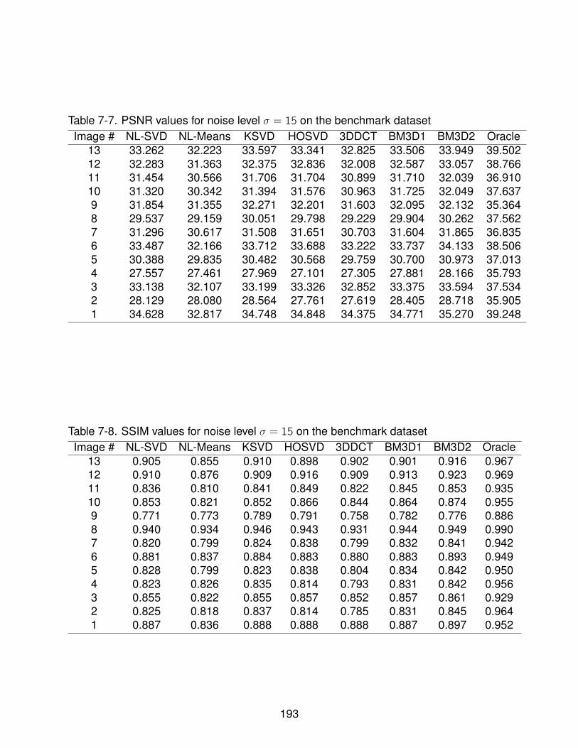
Table 7-7. PSNR values for noise level σ = 15 on the benchmark datasetImage # NL-SVD NL-Means KSVD HOSVD 3DDCT BM3D1 BM3D2 Oracle
13 33.262 32.223 33.597 33.341 32.825 33.506 33.949 39.50212 32.283 31.363 32.375 32.836 32.008 32.587 33.057 38.76611 31.454 30.566 31.706 31.704 30.899 31.710 32.039 36.91010 31.320 30.342 31.394 31.576 30.963 31.725 32.049 37.6379 31.854 31.355 32.271 32.201 31.603 32.095 32.132 35.3648 29.537 29.159 30.051 29.798 29.229 29.904 30.262 37.5627 31.296 30.617 31.508 31.651 30.703 31.604 31.865 36.8356 33.487 32.166 33.712 33.688 33.222 33.737 34.133 38.5065 30.388 29.835 30.482 30.568 29.759 30.700 30.973 37.0134 27.557 27.461 27.969 27.101 27.305 27.881 28.166 35.7933 33.138 32.107 33.199 33.326 32.852 33.375 33.594 37.5342 28.129 28.080 28.564 27.761 27.619 28.405 28.718 35.9051 34.628 32.817 34.748 34.848 34.375 34.771 35.270 39.248
Table 7-8. SSIM values for noise level σ = 15 on the benchmark datasetImage # NL-SVD NL-Means KSVD HOSVD 3DDCT BM3D1 BM3D2 Oracle
13 0.905 0.855 0.910 0.898 0.902 0.901 0.916 0.96712 0.910 0.876 0.909 0.916 0.909 0.913 0.923 0.96911 0.836 0.810 0.841 0.849 0.822 0.845 0.853 0.93510 0.853 0.821 0.852 0.866 0.844 0.864 0.874 0.9559 0.771 0.773 0.789 0.791 0.758 0.782 0.776 0.8868 0.940 0.934 0.946 0.943 0.931 0.944 0.949 0.9907 0.820 0.799 0.824 0.838 0.799 0.832 0.841 0.9426 0.881 0.837 0.884 0.883 0.880 0.883 0.893 0.9495 0.828 0.799 0.823 0.838 0.804 0.834 0.842 0.9504 0.823 0.826 0.835 0.814 0.793 0.831 0.842 0.9563 0.855 0.822 0.855 0.857 0.852 0.857 0.861 0.9292 0.825 0.818 0.837 0.814 0.785 0.831 0.845 0.9641 0.887 0.836 0.888 0.888 0.888 0.887 0.897 0.952
193
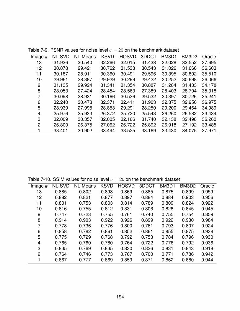
Table 7-9. PSNR values for noise level σ = 20 on the benchmark datasetImage # NL-SVD NL-Means KSVD HOSVD 3DDCT BM3D1 BM3D2 Oracle
13 31.936 30.540 32.266 32.015 31.433 32.028 32.552 37.69512 30.878 29.421 30.762 31.533 30.543 31.026 31.660 36.60311 30.187 28.911 30.360 30.491 29.596 30.395 30.802 35.51010 29.961 28.387 29.929 30.299 29.422 30.252 30.698 36.0669 31.135 29.924 31.341 31.354 30.887 31.284 31.433 34.1788 28.053 27.424 28.454 28.563 27.389 28.403 28.794 35.3187 30.098 28.931 30.166 30.536 29.532 30.397 30.726 35.2416 32.240 30.473 32.371 32.411 31.903 32.375 32.950 36.9755 28.939 27.995 28.853 29.291 28.250 29.200 29.464 34.9894 25.976 25.933 26.372 25.720 25.543 26.260 26.582 33.4343 32.009 30.357 32.005 32.166 31.740 32.138 32.498 36.2602 26.800 26.375 27.062 26.722 25.892 26.918 27.192 33.4851 33.401 30.902 33.494 33.525 33.169 33.430 34.075 37.971
Table 7-10. SSIM values for noise level σ = 20 on the benchmark datasetImage # NL-SVD NL-Means KSVD HOSVD 3DDCT BM3D1 BM3D2 Oracle
13 0.885 0.802 0.893 0.869 0.885 0.875 0.899 0.95912 0.882 0.821 0.877 0.897 0.884 0.884 0.903 0.95611 0.801 0.753 0.803 0.814 0.789 0.809 0.824 0.92210 0.816 0.755 0.812 0.831 0.806 0.828 0.845 0.9459 0.747 0.723 0.755 0.761 0.740 0.755 0.754 0.8598 0.914 0.903 0.922 0.926 0.899 0.922 0.930 0.9847 0.778 0.736 0.776 0.800 0.761 0.793 0.807 0.9246 0.858 0.782 0.861 0.852 0.861 0.855 0.875 0.9385 0.775 0.729 0.768 0.792 0.753 0.784 0.796 0.9304 0.765 0.760 0.780 0.764 0.722 0.776 0.792 0.9363 0.835 0.769 0.835 0.830 0.836 0.831 0.843 0.9182 0.764 0.746 0.773 0.767 0.700 0.771 0.786 0.9421 0.867 0.777 0.869 0.859 0.871 0.862 0.880 0.944
194
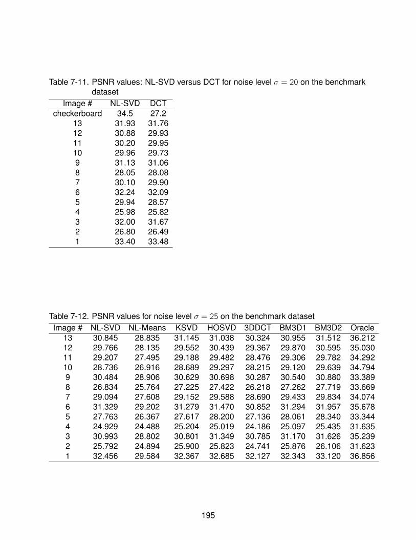
Table 7-11. PSNR values: NL-SVD versus DCT for noise level σ = 20 on the benchmarkdataset
Image # NL-SVD DCTcheckerboard 34.5 27.2
13 31.93 31.7612 30.88 29.9311 30.20 29.9510 29.96 29.739 31.13 31.068 28.05 28.087 30.10 29.906 32.24 32.095 29.94 28.574 25.98 25.823 32.00 31.672 26.80 26.491 33.40 33.48
Table 7-12. PSNR values for noise level σ = 25 on the benchmark datasetImage # NL-SVD NL-Means KSVD HOSVD 3DDCT BM3D1 BM3D2 Oracle
13 30.845 28.835 31.145 31.038 30.324 30.955 31.512 36.21212 29.766 28.135 29.552 30.439 29.367 29.870 30.595 35.03011 29.207 27.495 29.188 29.482 28.476 29.306 29.782 34.29210 28.736 26.916 28.689 29.297 28.215 29.120 29.639 34.7949 30.484 28.906 30.629 30.698 30.287 30.540 30.880 33.3898 26.834 25.764 27.225 27.422 26.218 27.262 27.719 33.6697 29.094 27.608 29.152 29.588 28.690 29.433 29.834 34.0746 31.329 29.202 31.279 31.470 30.852 31.294 31.957 35.6785 27.763 26.367 27.617 28.200 27.136 28.061 28.340 33.3444 24.929 24.488 25.204 25.019 24.186 25.097 25.435 31.6353 30.993 28.802 30.801 31.349 30.785 31.170 31.626 35.2392 25.792 24.894 25.900 25.823 24.741 25.876 26.106 31.6231 32.456 29.584 32.367 32.685 32.127 32.343 33.120 36.856
195
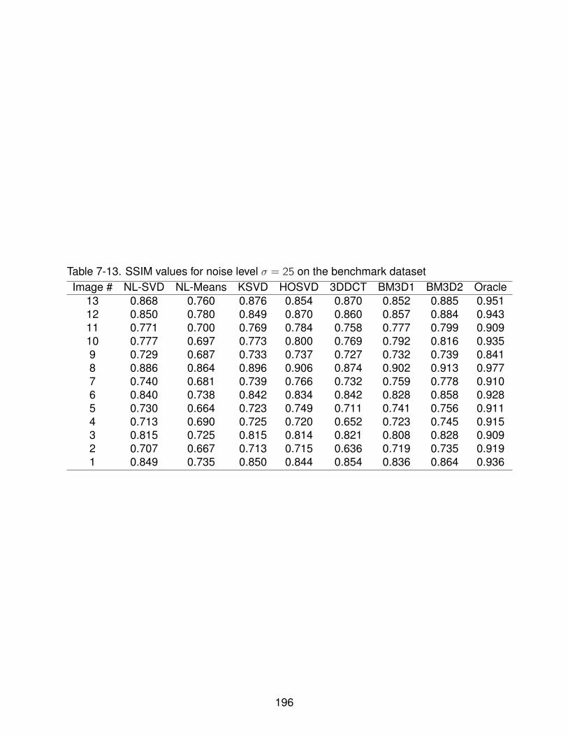
Table 7-13. SSIM values for noise level σ = 25 on the benchmark datasetImage # NL-SVD NL-Means KSVD HOSVD 3DDCT BM3D1 BM3D2 Oracle
13 0.868 0.760 0.876 0.854 0.870 0.852 0.885 0.95112 0.850 0.780 0.849 0.870 0.860 0.857 0.884 0.94311 0.771 0.700 0.769 0.784 0.758 0.777 0.799 0.90910 0.777 0.697 0.773 0.800 0.769 0.792 0.816 0.9359 0.729 0.687 0.733 0.737 0.727 0.732 0.739 0.8418 0.886 0.864 0.896 0.906 0.874 0.902 0.913 0.9777 0.740 0.681 0.739 0.766 0.732 0.759 0.778 0.9106 0.840 0.738 0.842 0.834 0.842 0.828 0.858 0.9285 0.730 0.664 0.723 0.749 0.711 0.741 0.756 0.9114 0.713 0.690 0.725 0.720 0.652 0.723 0.745 0.9153 0.815 0.725 0.815 0.814 0.821 0.808 0.828 0.9092 0.707 0.667 0.713 0.715 0.636 0.719 0.735 0.9191 0.849 0.735 0.850 0.844 0.854 0.836 0.864 0.936
196
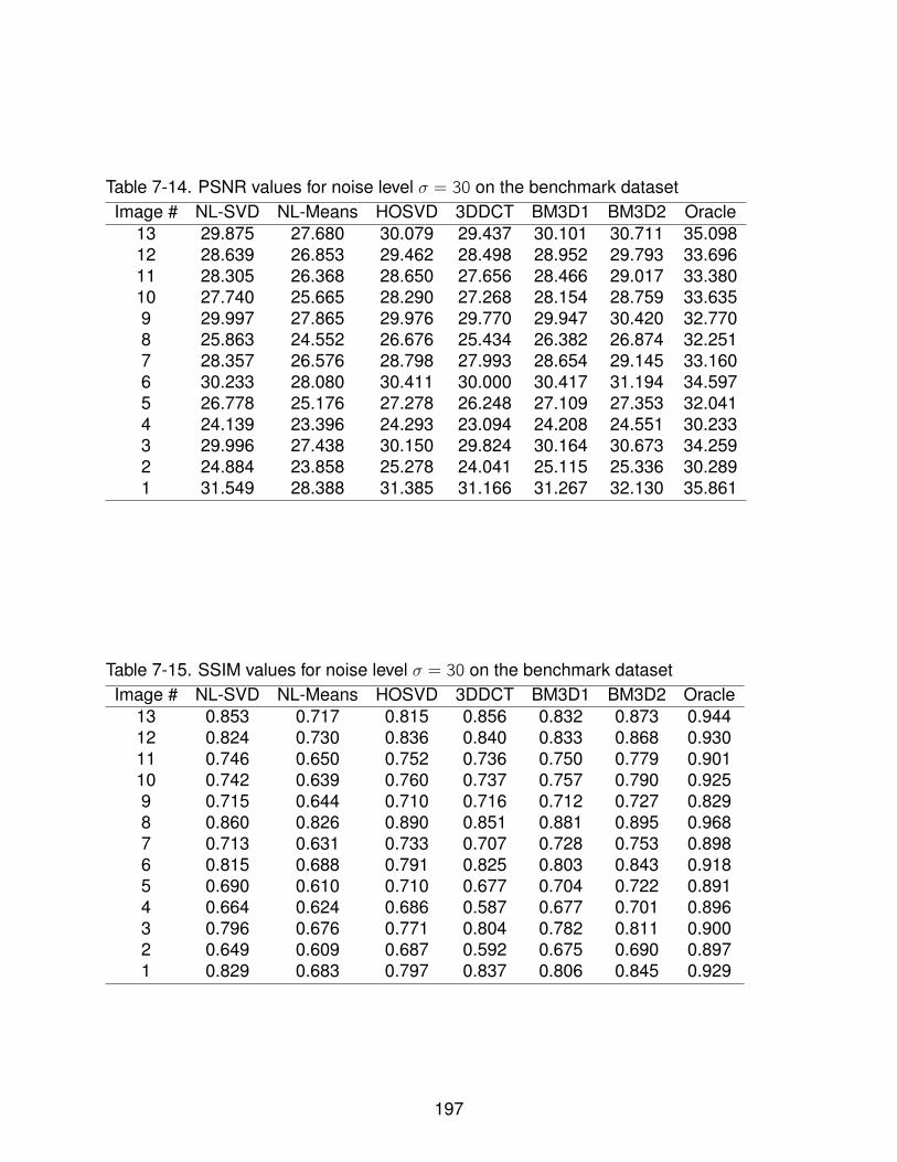
Table 7-14. PSNR values for noise level σ = 30 on the benchmark datasetImage # NL-SVD NL-Means HOSVD 3DDCT BM3D1 BM3D2 Oracle
13 29.875 27.680 30.079 29.437 30.101 30.711 35.09812 28.639 26.853 29.462 28.498 28.952 29.793 33.69611 28.305 26.368 28.650 27.656 28.466 29.017 33.38010 27.740 25.665 28.290 27.268 28.154 28.759 33.6359 29.997 27.865 29.976 29.770 29.947 30.420 32.7708 25.863 24.552 26.676 25.434 26.382 26.874 32.2517 28.357 26.576 28.798 27.993 28.654 29.145 33.1606 30.233 28.080 30.411 30.000 30.417 31.194 34.5975 26.778 25.176 27.278 26.248 27.109 27.353 32.0414 24.139 23.396 24.293 23.094 24.208 24.551 30.2333 29.996 27.438 30.150 29.824 30.164 30.673 34.2592 24.884 23.858 25.278 24.041 25.115 25.336 30.2891 31.549 28.388 31.385 31.166 31.267 32.130 35.861
Table 7-15. SSIM values for noise level σ = 30 on the benchmark datasetImage # NL-SVD NL-Means HOSVD 3DDCT BM3D1 BM3D2 Oracle
13 0.853 0.717 0.815 0.856 0.832 0.873 0.94412 0.824 0.730 0.836 0.840 0.833 0.868 0.93011 0.746 0.650 0.752 0.736 0.750 0.779 0.90110 0.742 0.639 0.760 0.737 0.757 0.790 0.9259 0.715 0.644 0.710 0.716 0.712 0.727 0.8298 0.860 0.826 0.890 0.851 0.881 0.895 0.9687 0.713 0.631 0.733 0.707 0.728 0.753 0.8986 0.815 0.688 0.791 0.825 0.803 0.843 0.9185 0.690 0.610 0.710 0.677 0.704 0.722 0.8914 0.664 0.624 0.686 0.587 0.677 0.701 0.8963 0.796 0.676 0.771 0.804 0.782 0.811 0.9002 0.649 0.609 0.687 0.592 0.675 0.690 0.8971 0.829 0.683 0.797 0.837 0.806 0.845 0.929
197
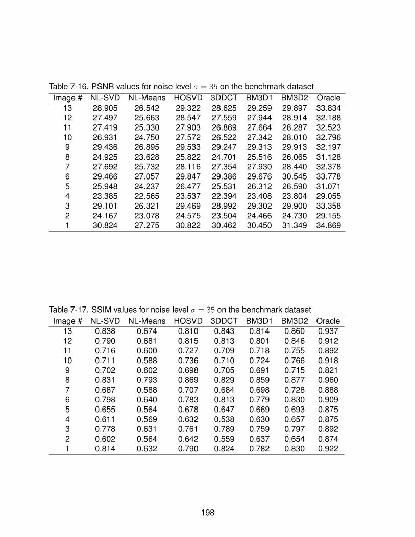
Table 7-16. PSNR values for noise level σ = 35 on the benchmark datasetImage # NL-SVD NL-Means HOSVD 3DDCT BM3D1 BM3D2 Oracle
13 28.905 26.542 29.322 28.625 29.259 29.897 33.83412 27.497 25.663 28.547 27.559 27.944 28.914 32.18811 27.419 25.330 27.903 26.869 27.664 28.287 32.52310 26.931 24.750 27.572 26.522 27.342 28.010 32.7969 29.436 26.895 29.533 29.247 29.313 29.913 32.1978 24.925 23.628 25.822 24.701 25.516 26.065 31.1287 27.692 25.732 28.116 27.354 27.930 28.440 32.3786 29.466 27.057 29.847 29.386 29.676 30.545 33.7785 25.948 24.237 26.477 25.531 26.312 26.590 31.0714 23.385 22.565 23.537 22.394 23.408 23.804 29.0553 29.101 26.321 29.469 28.992 29.302 29.900 33.3582 24.167 23.078 24.575 23.504 24.466 24.730 29.1551 30.824 27.275 30.822 30.462 30.450 31.349 34.869
Table 7-17. SSIM values for noise level σ = 35 on the benchmark datasetImage # NL-SVD NL-Means HOSVD 3DDCT BM3D1 BM3D2 Oracle
13 0.838 0.674 0.810 0.843 0.814 0.860 0.93712 0.790 0.681 0.815 0.813 0.801 0.846 0.91211 0.716 0.600 0.727 0.709 0.718 0.755 0.89210 0.711 0.588 0.736 0.710 0.724 0.766 0.9189 0.702 0.602 0.698 0.705 0.691 0.715 0.8218 0.831 0.793 0.869 0.829 0.859 0.877 0.9607 0.687 0.588 0.707 0.684 0.698 0.728 0.8886 0.798 0.640 0.783 0.813 0.779 0.830 0.9095 0.655 0.564 0.678 0.647 0.669 0.693 0.8754 0.611 0.569 0.632 0.538 0.630 0.657 0.8753 0.778 0.631 0.761 0.789 0.759 0.797 0.8922 0.602 0.564 0.642 0.559 0.637 0.654 0.8741 0.814 0.632 0.790 0.824 0.782 0.830 0.922
198
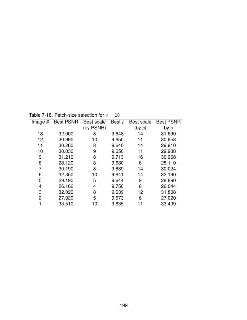
Table 7-18. Patch-size selection for σ = 20Image # Best PSNR Best scale Best ρ Best scale Best PSNR
(by PSNR) (by ρ) by ρ13 32.000 8 9.648 14 31.69012 30.990 10 9.650 11 30.95811 30.260 8 9.640 14 29.91010 30.030 9 9.650 11 29.9889 31.210 8 9.713 16 30.9688 28.120 8 9.680 6 28.1107 30.190 8 9.639 14 30.0246 32.350 10 9.641 14 32.1905 29.190 5 9.644 9 28.8904 26.166 4 9.756 6 26.0443 32.020 8 9.639 12 31.8082 27.020 5 9.673 6 27.0201 33.510 10 9.635 11 33.499
199
CHAPTER 8AUTOMATED SELECTION OF FILTER PARAMETERS
8.1 Introduction
Despite the vast body of literature on image denoising, relatively little work has
been done in the area of automatically choosing the filter parameters that yield optimal
filter performance. The typical denoising technique requires tuning parameters that are
critical for its optimal performance. In denoising experiments reported in contemporary
literature, the filter performance is usually measured using a full-reference image
quality measure (such as the MSE/PSNR or SSIM) between the denoised and the
original image. The parameters are picked so as to yield the optimal value of the
quality measure for a particular filter, but this requires knowledge of the original image
and is not extensible to real-world denoising situations. Hence we need criteria for
parameter selection that do not refer to the original image. In this chapter, we classify
these criteria into two types: (1) independence-based criteria that measure the degree
of independence between the denoised image and the residual, and (2) criteria that
measure how noisy the residual image is, without referring to the denoised image. We
contribute to and critique criteria of type (1), and proposed those of type (2). Our criteria
make the assumption that the noise is i.i.d. and additive, and that a loose lower-bound
on the noise variance is known.
The material in this chapter is based on the author’s published work in [170]1 . This
chapter is organized as follows: Section 8.2 reviews existing literature for filter parameter
selection, followed by a description of the proposed criteria in Section 8.3, experimental
results in Section 8.4 and discussion in Section 8.5.
1 Parts of the contents of this chapter have been reprinted with permission from: A.Rajwade, A. Rangarajan and A. Banerjee, ‘Automated Filter Parameter Selection usingMeasures of Noiseness’, Canadian Conference on Computer and Robot Vision, pages86-93, June 2010. c©2010, IEEE.
200
8.2 Literature Review on Automated Filter Parameter Selection
In PDE-based denoising, the choice of stopping time for the PDE evolution is a
crucial parameter. Some researchers propose to stop the PDE when the variance of
the residual equals the variance of the noise, which is assumed to be known [86], [171].
This method ignores higher order statistics of the noise. Others use a hypothesis test
between the empirical distribution of the residual and the true noise distribution [139] for
polynomial order selection in regression-based smoothing. However the exact variance
of the noise or its complete distribution is usually not known in practical situations.
A decorrelation-based criterion independently proposed in [172] and [173] does not
require any knowledge of the noise distribution except that the noise is independent
of the original signal. As per this criterion, the optimal filter parameter is chosen to be
one which minimizes the correlation coefficient between the denoised and the residual
images, regardless of the noise variance. This criterion however has some problems: (1)
in the limit of extreme over-smoothing or under-smoothing, the correlation coefficient is
undefined as the denoised image could become a constant image, (2) it is too global a
criterion (though using a sum of local measures is a ready alternative) and (3) it ignores
higher-order dependencies. A solution to the third issue is suggested by us in Section
8.3.
It should be noted that all the aforementioned criteria (as also the ones we suggest
in this chapter) are necessary but not sufficient for parameter selection. Gilboa et
al. [174] attempt to alleviate this by selecting a stopping time that seeks to maximize
the signal-to-noise-ratio (SNR) directly. Their method however requires an estimate
of the rate of change of the covariance between the residual and the noise w.r.t. the
filtering parameter. This estimate in turn requires full knowledge of the noise distribution.
Saddled with this method is the assumption that the covariance between the residual for
any image and the actual noise, can be estimated from a single noise-image (generated
from the same noise distribution) on which the filtering algorithm is run. This assumption
201

is not justified theoretically though experimental results are impressive (see [174] for
more details). Vanhamel et al. [175] propose a criterion that maximizes an estimate
of the correlation between the denoised image and the true, underlying image. This
estimate, however, can be computed only by using some assumptions that have only
experimental justification. In wavelet thresholding methods, risk based criteria have
been proposed for the optimal choice of the threshold for the wavelet coefficients. These
methods such as those in [113], or the SURE - Stein’s unbiased risk estimator from
[176], again require knowledge of the noise model including the noise variance value.
Recently, Brunet et al. have developed no-reference quality estimates of the MSE
between the denoised image and the true underlying image [141]. These estimates do
not require knowledge of the original image, but they do require knowledge of the noise
variance and obtain a rough, heuristic estimate of the covariance between the residual
and the noise. Moreover the performance of these estimates has been tested only on
Gaussian noise models.
8.3 Theory
8.3.1 Independence Measures
In what follows, we shall denoted the denoised image obtained by filtering a noisy
image I as D, its corresponding residual as R (note that R = I − D) and the true
image underlying I as J. As mentioned earlier, independence-based criteria have been
developed in image processing literature. In cases where a noisy signal is oversmoothed
(locally or globally), the residual image clearly shows the distinct features from the
image (referred to as ‘method noise’ in [2]). This is true even in those cases where
the noise is independent of the signal. Independence-based criteria are based on the
assumption that when the noisy image is filtered optimally, the residual would contain
mostly noise and very little signal and hence it would be independent of the denoised
image. It has been experimentally reported in [172] that the absolute correlation
coefficient (denoted as CC ) between D and R decreases almost monotonically as
202
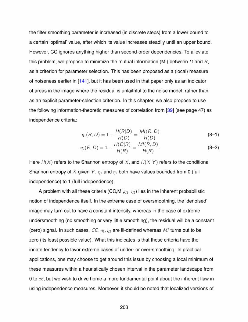
the filter smoothing parameter is increased (in discrete steps) from a lower bound to
a certain ‘optimal’ value, after which its value increases steadily until an upper bound.
However, CC ignores anything higher than second-order dependencies. To alleviate
this problem, we propose to minimize the mutual information (MI) between D and R,
as a criterion for parameter selection. This has been proposed as a (local) measure
of noiseness earlier in [141], but it has been used in that paper only as an indicator
of areas in the image where the residual is unfaithful to the noise model, rather than
as an explicit parameter-selection criterion. In this chapter, we also propose to use
the following information-theoretic measures of correlation from [39] (see page 47) as
independence criteria:
η1(R,D) = 1−H(R|D)H(D)
=MI (R,D)
H(D)(8–1)
η2(R,D) = 1−H(D|R)H(R)
=MI (R,D)
H(R). (8–2)
Here H(X ) refers to the Shannon entropy of X , and H(X |Y ) refers to the conditional
Shannon entropy of X given Y . η1 and η2 both have values bounded from 0 (full
independence) to 1 (full independence).
A problem with all these criteria (CC,MI,η1, η2) lies in the inherent probabilistic
notion of independence itself. In the extreme case of oversmoothing, the ‘denoised’
image may turn out to have a constant intensity, whereas in the case of extreme
undersmoothing (no smoothing or very little smoothing), the residual will be a constant
(zero) signal. In such cases, CC , η1, η2 are ill-defined whereas MI turns out to be
zero (its least possible value). What this indicates is that these criteria have the
innate tendency to favor extreme cases of under- or over-smoothing. In practical
applications, one may choose to get around this issue by choosing a local minimum of
these measures within a heuristically chosen interval in the parameter landscape from
0 to ∞, but we wish to drive home a more fundamental point about the inherent flaw in
using independence measures. Moreover, it should be noted that localized versions of
203
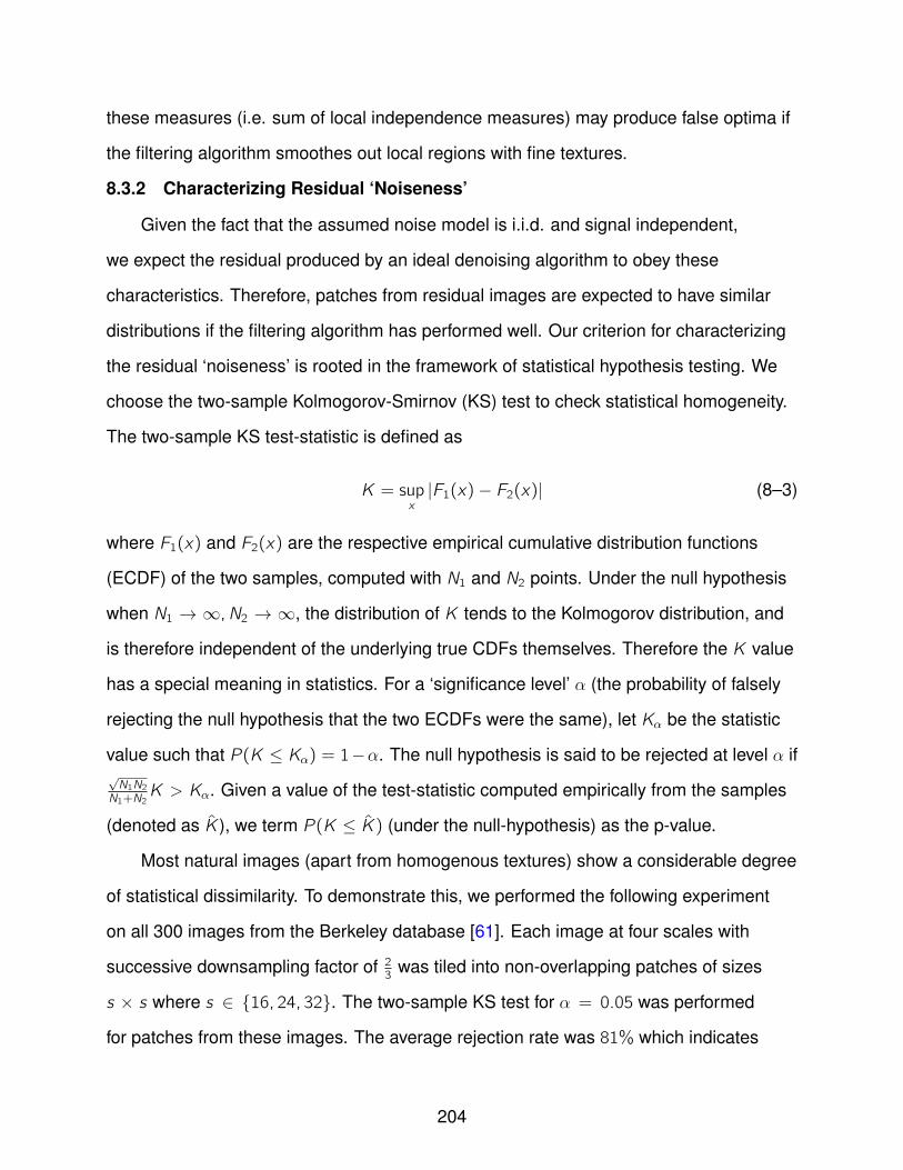
these measures (i.e. sum of local independence measures) may produce false optima if
the filtering algorithm smoothes out local regions with fine textures.
8.3.2 Characterizing Residual ‘Noiseness’
Given the fact that the assumed noise model is i.i.d. and signal independent,
we expect the residual produced by an ideal denoising algorithm to obey these
characteristics. Therefore, patches from residual images are expected to have similar
distributions if the filtering algorithm has performed well. Our criterion for characterizing
the residual ‘noiseness’ is rooted in the framework of statistical hypothesis testing. We
choose the two-sample Kolmogorov-Smirnov (KS) test to check statistical homogeneity.
The two-sample KS test-statistic is defined as
K = supx
|F1(x)− F2(x)| (8–3)
where F1(x) and F2(x) are the respective empirical cumulative distribution functions
(ECDF) of the two samples, computed with N1 and N2 points. Under the null hypothesis
when N1 → ∞,N2 → ∞, the distribution of K tends to the Kolmogorov distribution, and
is therefore independent of the underlying true CDFs themselves. Therefore the K value
has a special meaning in statistics. For a ‘significance level’ α (the probability of falsely
rejecting the null hypothesis that the two ECDFs were the same), let Kα be the statistic
value such that P(K ≤ Kα) = 1−α. The null hypothesis is said to be rejected at level α if√N1N2N1+N2
K > Kα. Given a value of the test-statistic computed empirically from the samples
(denoted as K ), we term P(K ≤ K) (under the null-hypothesis) as the p-value.
Most natural images (apart from homogenous textures) show a considerable degree
of statistical dissimilarity. To demonstrate this, we performed the following experiment
on all 300 images from the Berkeley database [61]. Each image at four scales with
successive downsampling factor of 23
was tiled into non-overlapping patches of sizes
s × s where s ∈ 16, 24, 32. The two-sample KS test for α = 0.05 was performed
for patches from these images. The average rejection rate was 81% which indicates
204
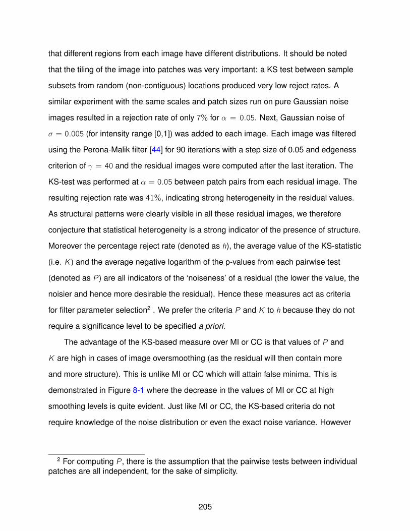
that different regions from each image have different distributions. It should be noted
that the tiling of the image into patches was very important: a KS test between sample
subsets from random (non-contiguous) locations produced very low reject rates. A
similar experiment with the same scales and patch sizes run on pure Gaussian noise
images resulted in a rejection rate of only 7% for α = 0.05. Next, Gaussian noise of
σ = 0.005 (for intensity range [0,1]) was added to each image. Each image was filtered
using the Perona-Malik filter [44] for 90 iterations with a step size of 0.05 and edgeness
criterion of γ = 40 and the residual images were computed after the last iteration. The
KS-test was performed at α = 0.05 between patch pairs from each residual image. The
resulting rejection rate was 41%, indicating strong heterogeneity in the residual values.
As structural patterns were clearly visible in all these residual images, we therefore
conjecture that statistical heterogeneity is a strong indicator of the presence of structure.
Moreover the percentage reject rate (denoted as h), the average value of the KS-statistic
(i.e. K ) and the average negative logarithm of the p-values from each pairwise test
(denoted as P) are all indicators of the ‘noiseness’ of a residual (the lower the value, the
noisier and hence more desirable the residual). Hence these measures act as criteria
for filter parameter selection2 . We prefer the criteria P and K to h because they do not
require a significance level to be specified a priori.
The advantage of the KS-based measure over MI or CC is that values of P and
K are high in cases of image oversmoothing (as the residual will then contain more
and more structure). This is unlike MI or CC which will attain false minima. This is
demonstrated in Figure 8-1 where the decrease in the values of MI or CC at high
smoothing levels is quite evident. Just like MI or CC, the KS-based criteria do not
require knowledge of the noise distribution or even the exact noise variance. However
2 For computing P, there is the assumption that the pairwise tests between individualpatches are all independent, for the sake of simplicity.
205
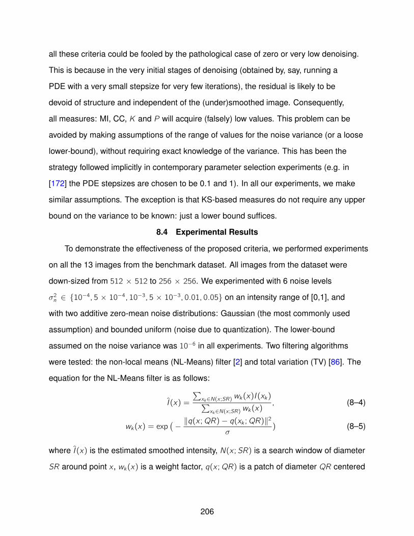
all these criteria could be fooled by the pathological case of zero or very low denoising.
This is because in the very initial stages of denoising (obtained by, say, running a
PDE with a very small stepsize for very few iterations), the residual is likely to be
devoid of structure and independent of the (under)smoothed image. Consequently,
all measures: MI, CC, K and P will acquire (falsely) low values. This problem can be
avoided by making assumptions of the range of values for the noise variance (or a loose
lower-bound), without requiring exact knowledge of the variance. This has been the
strategy followed implicitly in contemporary parameter selection experiments (e.g. in
[172] the PDE stepsizes are chosen to be 0.1 and 1). In all our experiments, we make
similar assumptions. The exception is that KS-based measures do not require any upper
bound on the variance to be known: just a lower bound suffices.
8.4 Experimental Results
To demonstrate the effectiveness of the proposed criteria, we performed experiments
on all the 13 images from the benchmark dataset. All images from the dataset were
down-sized from 512 × 512 to 256 × 256. We experimented with 6 noise levels
σ2n ∈ 10−4, 5 × 10⁻⁴, 10−3, 5 × 10⁻³, 0.01, 0.05 on an intensity range of [0,1], and
with two additive zero-mean noise distributions: Gaussian (the most commonly used
assumption) and bounded uniform (noise due to quantization). The lower-bound
assumed on the noise variance was 10−6 in all experiments. Two filtering algorithms
were tested: the non-local means (NL-Means) filter [2] and total variation (TV) [86]. The
equation for the NL-Means filter is as follows:
I (x) =
∑xk∈N(x ;SR) wk(x)I (xk)∑xk∈N(x ;SR) wk(x)
, (8–4)
wk(x) = exp(− ‖q(x ;QR)− q(xk ;QR)‖2
σ) (8–5)
where I (x) is the estimated smoothed intensity, N(x ;SR) is a search window of diameter
SR around point x , wk(x) is a weight factor, q(x ;QR) is a patch of diameter QR centered
206
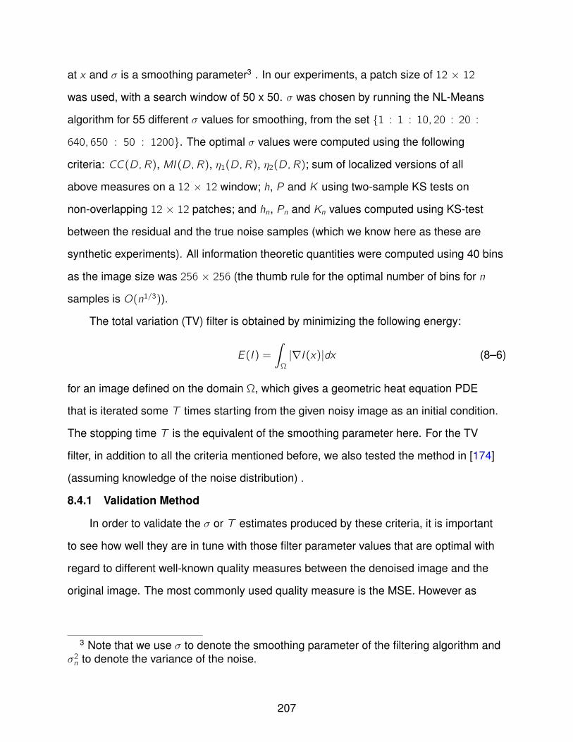
at x and σ is a smoothing parameter3 . In our experiments, a patch size of 12 × 12
was used, with a search window of 50 x 50. σ was chosen by running the NL-Means
algorithm for 55 different σ values for smoothing, from the set 1 : 1 : 10, 20 : 20 :
640, 650 : 50 : 1200. The optimal σ values were computed using the following
criteria: CC(D,R), MI (D,R), η1(D,R), η2(D,R); sum of localized versions of all
above measures on a 12 × 12 window; h, P and K using two-sample KS tests on
non-overlapping 12 × 12 patches; and hn, Pn and Kn values computed using KS-test
between the residual and the true noise samples (which we know here as these are
synthetic experiments). All information theoretic quantities were computed using 40 bins
as the image size was 256 × 256 (the thumb rule for the optimal number of bins for n
samples is O(n1/3)).
The total variation (TV) filter is obtained by minimizing the following energy:
E(I ) =
∫Ω
|∇I (x)|dx (8–6)
for an image defined on the domain Ω, which gives a geometric heat equation PDE
that is iterated some T times starting from the given noisy image as an initial condition.
The stopping time T is the equivalent of the smoothing parameter here. For the TV
filter, in addition to all the criteria mentioned before, we also tested the method in [174]
(assuming knowledge of the noise distribution) .
8.4.1 Validation Method
In order to validate the σ or T estimates produced by these criteria, it is important
to see how well they are in tune with those filter parameter values that are optimal with
regard to different well-known quality measures between the denoised image and the
original image. The most commonly used quality measure is the MSE. However as
3 Note that we use σ to denote the smoothing parameter of the filtering algorithm andσ2n to denote the variance of the noise.
207
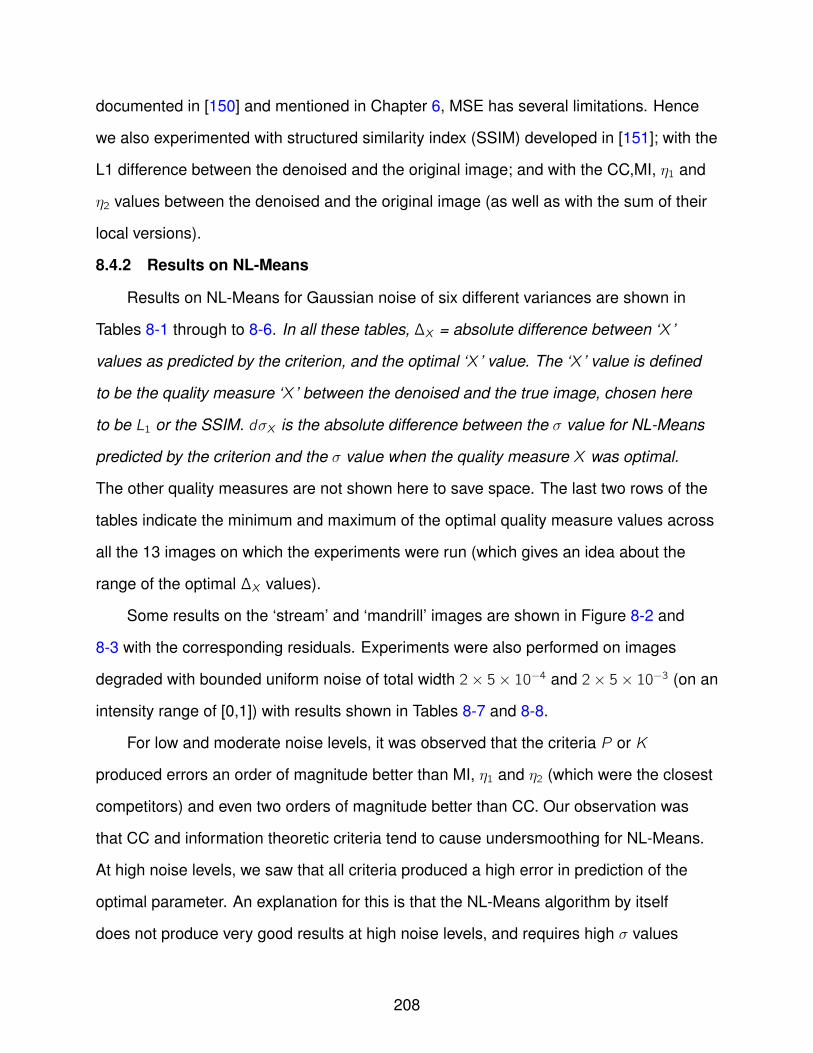
documented in [150] and mentioned in Chapter 6, MSE has several limitations. Hence
we also experimented with structured similarity index (SSIM) developed in [151]; with the
L1 difference between the denoised and the original image; and with the CC,MI, η1 and
η2 values between the denoised and the original image (as well as with the sum of their
local versions).
8.4.2 Results on NL-Means
Results on NL-Means for Gaussian noise of six different variances are shown in
Tables 8-1 through to 8-6. In all these tables, ∆X = absolute difference between ‘X ’
values as predicted by the criterion, and the optimal ‘X ’ value. The ‘X ’ value is defined
to be the quality measure ‘X ’ between the denoised and the true image, chosen here
to be L1 or the SSIM. dσX is the absolute difference between the σ value for NL-Means
predicted by the criterion and the σ value when the quality measure X was optimal.
The other quality measures are not shown here to save space. The last two rows of the
tables indicate the minimum and maximum of the optimal quality measure values across
all the 13 images on which the experiments were run (which gives an idea about the
range of the optimal ∆X values).
Some results on the ‘stream’ and ‘mandrill’ images are shown in Figure 8-2 and
8-3 with the corresponding residuals. Experiments were also performed on images
degraded with bounded uniform noise of total width 2× 5× 10−4 and 2× 5× 10−3 (on an
intensity range of [0,1]) with results shown in Tables 8-7 and 8-8.
For low and moderate noise levels, it was observed that the criteria P or K
produced errors an order of magnitude better than MI, η1 and η2 (which were the closest
competitors) and even two orders of magnitude better than CC. Our observation was
that CC and information theoretic criteria tend to cause undersmoothing for NL-Means.
At high noise levels, we saw that all criteria produced a high error in prediction of the
optimal parameter. An explanation for this is that the NL-Means algorithm by itself
does not produce very good results at high noise levels, and requires high σ values
208
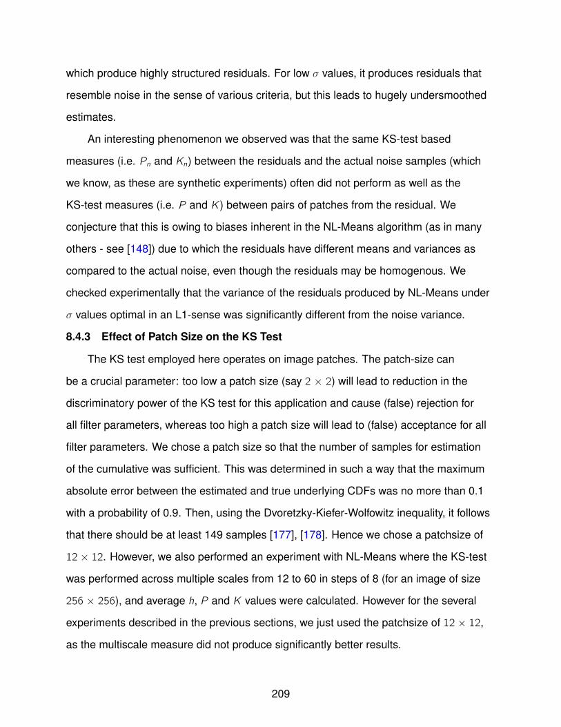
which produce highly structured residuals. For low σ values, it produces residuals that
resemble noise in the sense of various criteria, but this leads to hugely undersmoothed
estimates.
An interesting phenomenon we observed was that the same KS-test based
measures (i.e. Pn and Kn) between the residuals and the actual noise samples (which
we know, as these are synthetic experiments) often did not perform as well as the
KS-test measures (i.e. P and K ) between pairs of patches from the residual. We
conjecture that this is owing to biases inherent in the NL-Means algorithm (as in many
others - see [148]) due to which the residuals have different means and variances as
compared to the actual noise, even though the residuals may be homogenous. We
checked experimentally that the variance of the residuals produced by NL-Means under
σ values optimal in an L1-sense was significantly different from the noise variance.
8.4.3 Effect of Patch Size on the KS Test
The KS test employed here operates on image patches. The patch-size can
be a crucial parameter: too low a patch size (say 2 × 2) will lead to reduction in the
discriminatory power of the KS test for this application and cause (false) rejection for
all filter parameters, whereas too high a patch size will lead to (false) acceptance for all
filter parameters. We chose a patch size so that the number of samples for estimation
of the cumulative was sufficient. This was determined in such a way that the maximum
absolute error between the estimated and true underlying CDFs was no more than 0.1
with a probability of 0.9. Then, using the Dvoretzky-Kiefer-Wolfowitz inequality, it follows
that there should be at least 149 samples [177], [178]. Hence we chose a patchsize of
12 × 12. However, we also performed an experiment with NL-Means where the KS-test
was performed across multiple scales from 12 to 60 in steps of 8 (for an image of size
256 × 256), and average h, P and K values were calculated. However for the several
experiments described in the previous sections, we just used the patchsize of 12 × 12,
as the multiscale measure did not produce significantly better results.
209
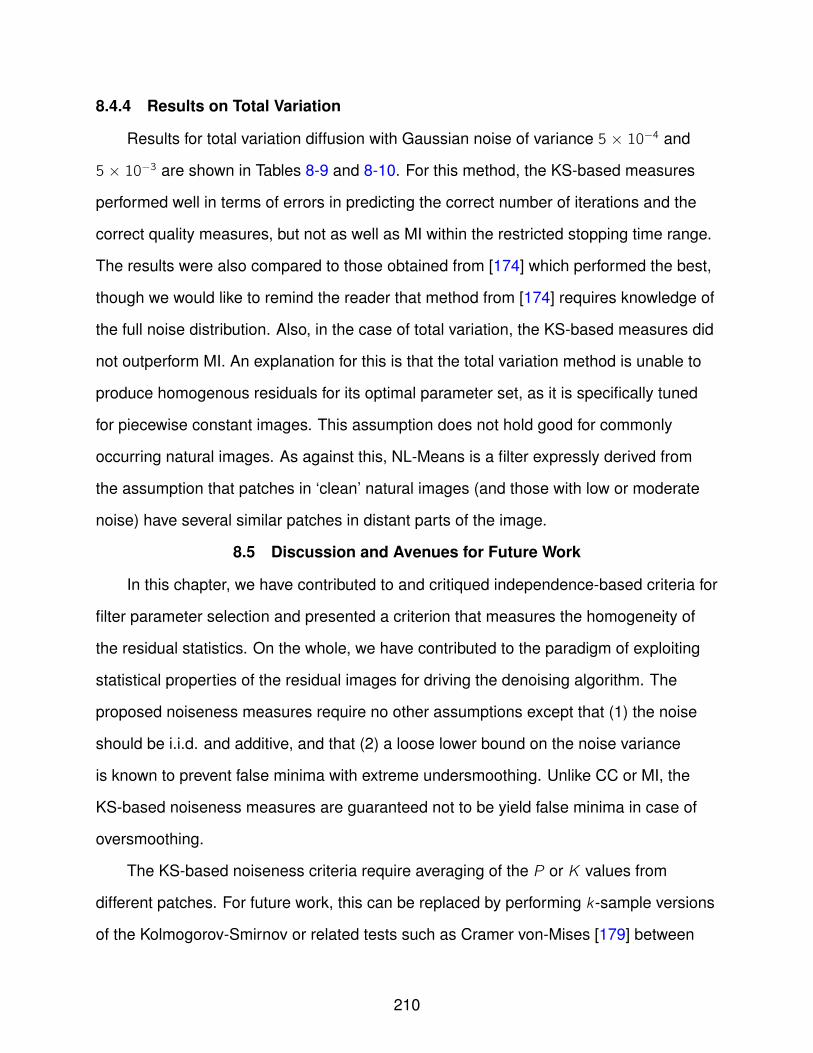
8.4.4 Results on Total Variation
Results for total variation diffusion with Gaussian noise of variance 5 × 10⁻⁴ and
5 × 10⁻³ are shown in Tables 8-9 and 8-10. For this method, the KS-based measures
performed well in terms of errors in predicting the correct number of iterations and the
correct quality measures, but not as well as MI within the restricted stopping time range.
The results were also compared to those obtained from [174] which performed the best,
though we would like to remind the reader that method from [174] requires knowledge of
the full noise distribution. Also, in the case of total variation, the KS-based measures did
not outperform MI. An explanation for this is that the total variation method is unable to
produce homogenous residuals for its optimal parameter set, as it is specifically tuned
for piecewise constant images. This assumption does not hold good for commonly
occurring natural images. As against this, NL-Means is a filter expressly derived from
the assumption that patches in ‘clean’ natural images (and those with low or moderate
noise) have several similar patches in distant parts of the image.
8.5 Discussion and Avenues for Future Work
In this chapter, we have contributed to and critiqued independence-based criteria for
filter parameter selection and presented a criterion that measures the homogeneity of
the residual statistics. On the whole, we have contributed to the paradigm of exploiting
statistical properties of the residual images for driving the denoising algorithm. The
proposed noiseness measures require no other assumptions except that (1) the noise
should be i.i.d. and additive, and that (2) a loose lower bound on the noise variance
is known to prevent false minima with extreme undersmoothing. Unlike CC or MI, the
KS-based noiseness measures are guaranteed not to be yield false minima in case of
oversmoothing.
The KS-based noiseness criteria require averaging of the P or K values from
different patches. For future work, this can be replaced by performing k-sample versions
of the Kolmogorov-Smirnov or related tests such as Cramer von-Mises [179] between
210
individual patches versus a pooled sample containing the entire residual image. This will
produce a single K or P value for the whole image.
The assumption of i.i.d. noise may not hold in some denoising scenarios. In case
of a zero-mean Gaussian noise model with intensity dependent variances, a heuristic
approach would be to normalize the residuals suitably using feedback from the denoised
intensity values (regarding them as the ‘true’ image values) and then running the
KS-tests. The efficacy of this approach needs to be tested on denoising algorithms that
are capable of handling intensity dependent noise. In case the noise obeys a Poisson
distribution (which is neither fully additive nor multiplicative), there are two ways to
proceed: either apply a variance stabilizer transformation [180] which converts the data
into that corrupted by Gaussian noise with variance of one, or else suitably change the
definition of the residual itself.
Moreover, the existence of a universally optimal parameter selector is not yet
established: different criteria may perform better or worse for different denoising
algorithms or with different assumptions on the noise model. This is, as per our
survey of the literature, an unsolved problem in image processing. Lastly, despite
encouraging experimental results, there is no established theoretical relationship
between the performance of noiseness criteria for filter parameter selection and the
‘ideal’ parameters in terms of image quality criteria like MSE. A detailed study of
risk-based criteria such as those in [113] may be important in this context.
211
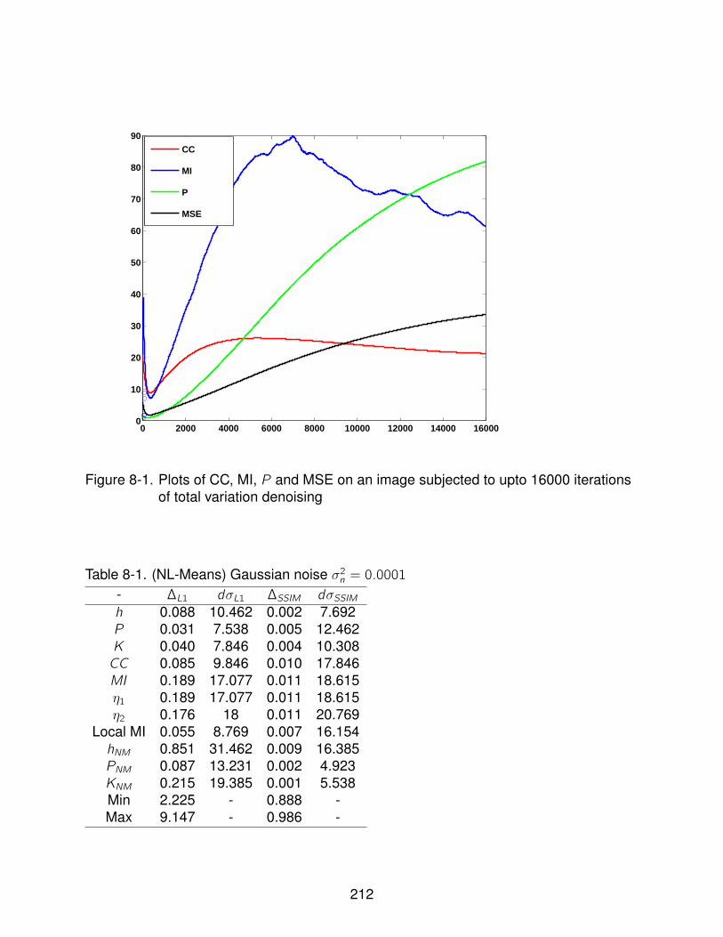
0 2000 4000 6000 8000 10000 12000 14000 160000
10
20
30
40
50
60
70
80
90
CC
MI
P
MSE
Figure 8-1. Plots of CC, MI, P and MSE on an image subjected to upto 16000 iterationsof total variation denoising
Table 8-1. (NL-Means) Gaussian noise σ2n = 0.0001- ∆L1 dσL1 ∆SSIM dσSSIMh 0.088 10.462 0.002 7.692P 0.031 7.538 0.005 12.462K 0.040 7.846 0.004 10.308CC 0.085 9.846 0.010 17.846MI 0.189 17.077 0.011 18.615η1 0.189 17.077 0.011 18.615η2 0.176 18 0.011 20.769
Local MI 0.055 8.769 0.007 16.154hNM 0.851 31.462 0.009 16.385PNM 0.087 13.231 0.002 4.923KNM 0.215 19.385 0.001 5.538Min 2.225 - 0.888 -Max 9.147 - 0.986 -
212
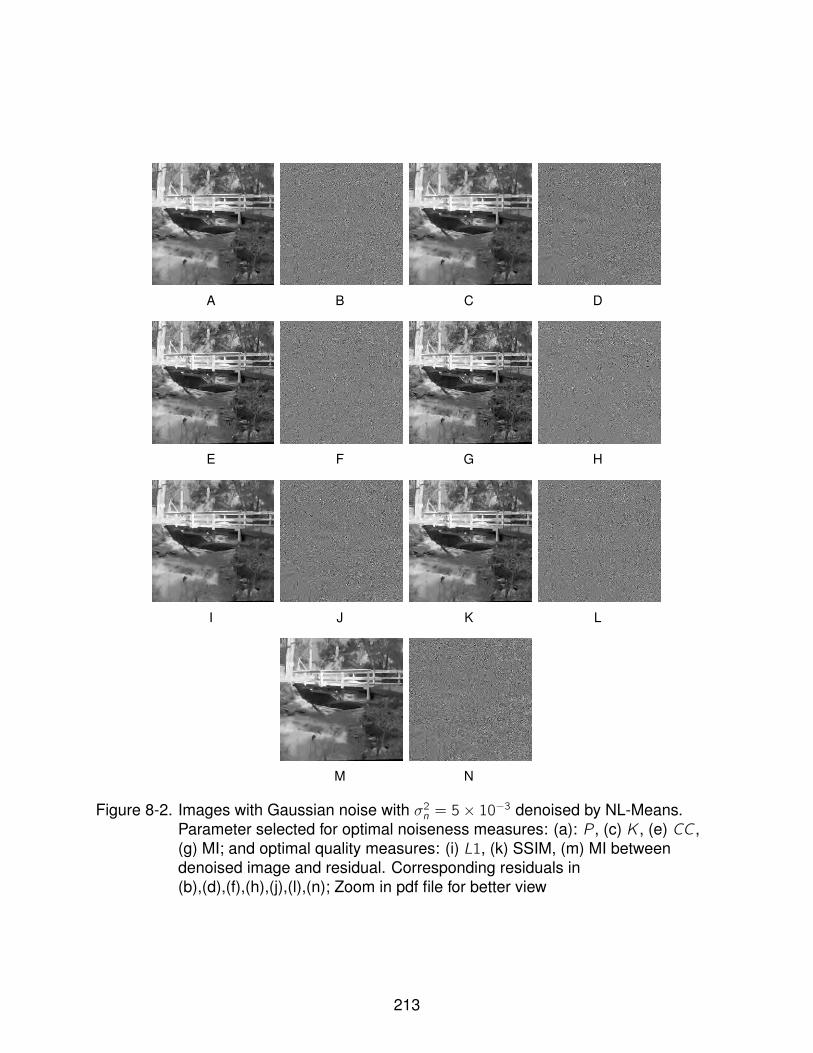
A B C D
E F G H
I J K L
M N
Figure 8-2. Images with Gaussian noise with σ2n = 5× 10⁻³ denoised by NL-Means.Parameter selected for optimal noiseness measures: (a): P, (c) K , (e) CC ,(g) MI; and optimal quality measures: (i) L1, (k) SSIM, (m) MI betweendenoised image and residual. Corresponding residuals in(b),(d),(f),(h),(j),(l),(n); Zoom in pdf file for better view
213

A B C D
E F G H
I J K L
M N
Figure 8-3. Images with Gaussian noise with σ2n = 5× 10⁻³ denoised by NL-Means.Parameter selected for optimal noiseness measures: (a): P, (c) K , (e) CC ,(g) MI; and optimal quality measures: (i) L1, (k) SSIM, (m) MI betweendenoised image and residual. Corresponding residuals in(b),(d),(f),(h),(j),(l),(n); Zoom in pdf file for better view
214
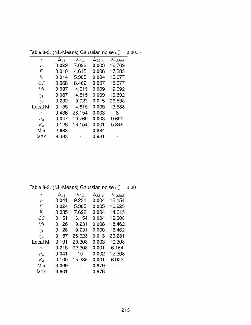
Table 8-2. (NL-Means) Gaussian noise σ2n = 0.0005- ∆L1 dσL1 ∆SSIM dσSSIMh 0.029 7.692 0.003 12.769P 0.010 4.615 0.006 17.385K 0.014 5.385 0.004 15.077CC 0.068 8.462 0.007 15.077MI 0.087 14.615 0.009 19.692η1 0.087 14.615 0.009 19.692η2 0.232 19.923 0.015 26.538
Local MI 0.155 14.615 0.005 13.538hn 0.436 28.154 0.003 8Pn 0.047 10.769 0.003 9.692Kn 0.128 16.154 0.001 5.846Min 2.683 - 0.884 -Max 9.383 - 0.981 -
Table 8-3. (NL-Means) Gaussian noise σ2n = 0.001- ∆L1 dσL1 ∆SSIM dσSSIMh 0.041 9.231 0.004 16.154P 0.024 5.385 0.005 16.923K 0.035 7.692 0.004 14.615CC 0.151 16.154 0.004 12.308MI 0.126 19.231 0.008 18.462η1 0.126 19.231 0.008 18.462η2 0.157 26.923 0.013 29.231
Local MI 0.191 20.308 0.003 10.308hn 0.218 22.308 0.001 6.154Pn 0.041 10 0.002 12.308Kn 0.100 15.385 0.001 6.923Min 3.069 - 0.879 -Max 9.601 - 0.976 -
215

Table 8-4. (NL-Means) Gaussian noise σ2n = 0.005- ∆L1 dσL1 ∆SSIM dσSSIMh 0.206 33.846 0.003 24.615P 0.207 33.846 0.003 24.615K 0.488 43 0.005 33.769CC 2.253 92.308 0.034 55.385MI 2.677 79.538 0.054 67.231η1 2.720 81.077 0.054 68.769η2 2.119 105.231 0.053 105.231
Local MI 3.889 107.846 0.069 74hn 1.337 38 0.032 38Pn 1.335 33.538 0.033 36.615Kn 1.336 33.538 0.034 42.769Min 4.838 - 0.791 -Max 10.695 - 0.955 -
Table 8-5. (NL-Means) Gaussian noise σ2n = 0.01- ∆L1 dσL1 ∆SSIM dσSSIMh 12.121 226.692 0.202 177.462P 12.121 226.692 0.202 177.462K 12.121 226.692 0.202 177.462CC 8.886 207.154 0.149 157.923MI 11.701 224.462 0.195 175.231η1 11.701 224.462 0.195 175.231η2 6.218 200 0.119 163.077
Local MI 12.121 226.692 0.202 177.462hn 1.891 60.923 0.045 64Pn 3.642 86.462 0.081 108Kn 3.649 88 0.082 115.692Min 6.285 - 0.735 -Max 11.661 - 0.933 -
216
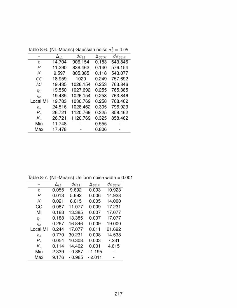
Table 8-6. (NL-Means) Gaussian noise σ2n = 0.05- ∆L1 dσL1 ∆SSIM dσSSIMh 14.704 906.154 0.183 643.846P 11.290 838.462 0.140 576.154K 9.597 805.385 0.118 543.077CC 18.959 1020 0.249 757.692MI 19.435 1026.154 0.253 763.846η1 19.550 1027.692 0.255 765.385η2 19.435 1026.154 0.253 763.846
Local MI 19.783 1030.769 0.258 768.462hn 24.516 1028.462 0.305 796.923Pn 26.721 1120.769 0.325 858.462Kn 26.721 1120.769 0.325 858.462Min 11.748 - 0.555 -Max 17.478 - 0.806 -
Table 8-7. (NL-Means) Uniform noise width = 0.001- ∆L1 dσL1 ∆SSIM dσSSIMh 0.055 9.692 0.003 10.923P 0.013 5.692 0.006 14.923K 0.021 6.615 0.005 14.000
CC 0.087 11.077 0.009 17.231MI 0.188 13.385 0.007 17.077η1 0.188 13.385 0.007 17.077η2 0.267 16.846 0.009 19.000
Local MI 0.244 17.077 0.011 21.692hn 0.770 30.231 0.008 14.538Pn 0.054 10.308 0.003 7.231Kn 0.114 14.462 0.001 4.615Min 2.339 - 0.887 - 1.195 -Max 9.176 - 0.985 - 2.011 -
217
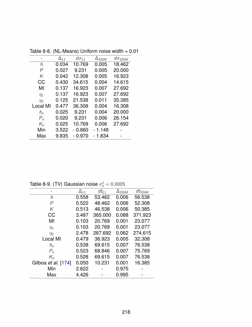
Table 8-8. (NL-Means) Uniform noise width = 0.01- ∆L1 dσL1 ∆SSIM dσSSIMh 0.034 10.769 0.005 18.462P 0.027 9.231 0.005 20.000K 0.042 12.308 0.005 16.923
CC 0.430 34.615 0.004 14.615MI 0.137 16.923 0.007 27.692η1 0.137 16.923 0.007 27.692η2 0.125 21.538 0.011 35.385
Local MI 0.477 36.308 0.004 16.308hn 0.025 9.231 0.004 20.000Pn 0.020 9.231 0.006 26.154Kn 0.025 10.769 0.006 27.692Min 3.522 - 0.860 - 1.148 -Max 9.835 - 0.970 - 1.834 -
Table 8-9. (TV) Gaussian noise σ2n = 0.0005- ∆L1 dtL1 ∆SSIM dtSSIMh 0.558 53.462 0.006 56.538P 0.522 48.462 0.006 52.308K 0.513 46.538 0.006 50.385
CC 3.487 365.000 0.088 371.923MI 0.103 20.769 0.001 23.077η1 0.103 20.769 0.001 23.077η2 2.478 267.692 0.062 274.615
Local MI 0.479 36.923 0.005 32.308hn 0.538 69.615 0.007 76.538Pn 0.523 68.846 0.007 75.769Kn 0.528 69.615 0.007 76.538
Gilboa et al. [174] 0.050 10.231 0.001 16.385Min 2.622 - 0.975 -Max 4.426 - 0.995 -
218
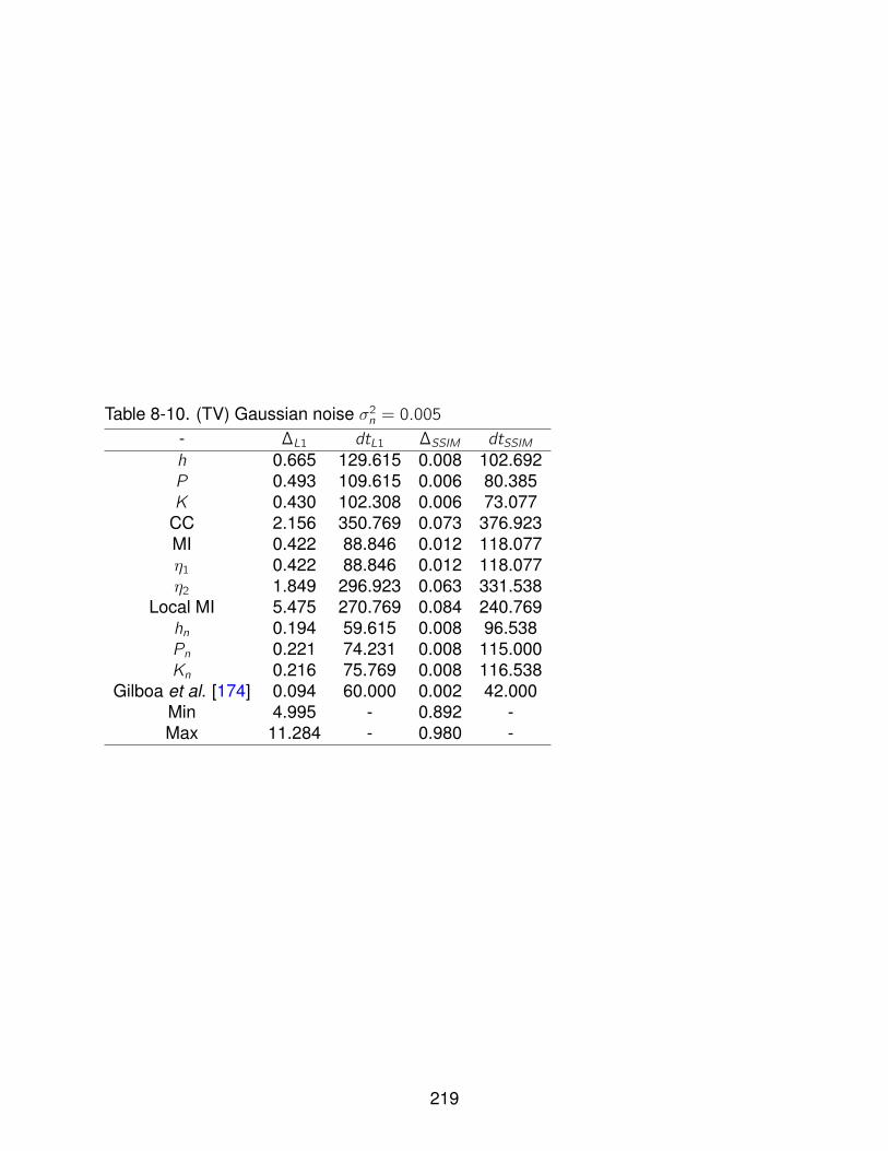
Table 8-10. (TV) Gaussian noise σ2n = 0.005- ∆L1 dtL1 ∆SSIM dtSSIMh 0.665 129.615 0.008 102.692P 0.493 109.615 0.006 80.385K 0.430 102.308 0.006 73.077
CC 2.156 350.769 0.073 376.923MI 0.422 88.846 0.012 118.077η1 0.422 88.846 0.012 118.077η2 1.849 296.923 0.063 331.538
Local MI 5.475 270.769 0.084 240.769hn 0.194 59.615 0.008 96.538Pn 0.221 74.231 0.008 115.000Kn 0.216 75.769 0.008 116.538
Gilboa et al. [174] 0.094 60.000 0.002 42.000Min 4.995 - 0.892 -Max 11.284 - 0.980 -
219
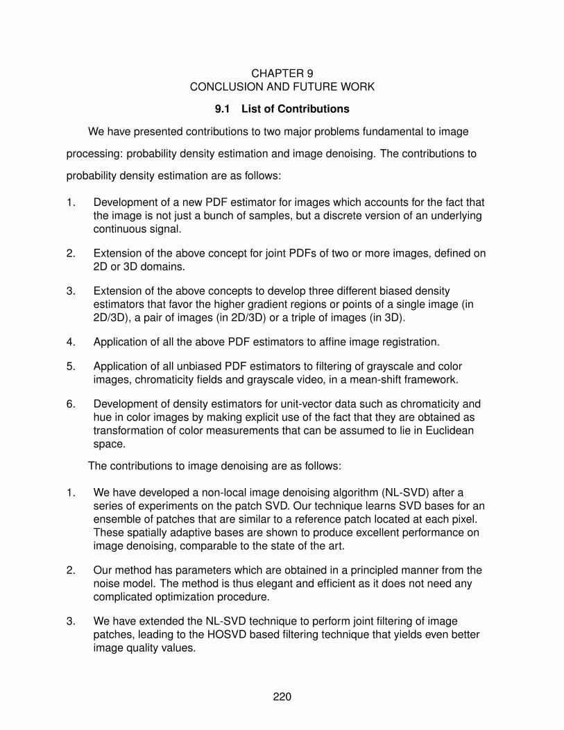
CHAPTER 9CONCLUSION AND FUTURE WORK
9.1 List of Contributions
We have presented contributions to two major problems fundamental to image
processing: probability density estimation and image denoising. The contributions to
probability density estimation are as follows:
1. Development of a new PDF estimator for images which accounts for the fact thatthe image is not just a bunch of samples, but a discrete version of an underlyingcontinuous signal.
2. Extension of the above concept for joint PDFs of two or more images, defined on2D or 3D domains.
3. Extension of the above concepts to develop three different biased densityestimators that favor the higher gradient regions or points of a single image (in2D/3D), a pair of images (in 2D/3D) or a triple of images (in 3D).
4. Application of all the above PDF estimators to affine image registration.
5. Application of all unbiased PDF estimators to filtering of grayscale and colorimages, chromaticity fields and grayscale video, in a mean-shift framework.
6. Development of density estimators for unit-vector data such as chromaticity andhue in color images by making explicit use of the fact that they are obtained astransformation of color measurements that can be assumed to lie in Euclideanspace.
The contributions to image denoising are as follows:
1. We have developed a non-local image denoising algorithm (NL-SVD) after aseries of experiments on the patch SVD. Our technique learns SVD bases for anensemble of patches that are similar to a reference patch located at each pixel.These spatially adaptive bases are shown to produce excellent performance onimage denoising, comparable to the state of the art.
2. Our method has parameters which are obtained in a principled manner from thenoise model. The method is thus elegant and efficient as it does not need anycomplicated optimization procedure.
3. We have extended the NL-SVD technique to perform joint filtering of imagepatches, leading to the HOSVD based filtering technique that yields even betterimage quality values.
220
4. We have also presented a new statistical criterion for automated filter parameterselection and used it to obtain the smoothing parameter in the NLMeans algorithmwithout reference to the true image.
9.2 Future Work
Future work on the probability density estimator has been outlined in Section 3.4.
Here, we leave behind pointers to possible future extensions of our work in image
denoising.
9.2.1 Trying to Reach the Oracle
The ultimate aim of several of the procedures reported in Chapter 7 was to obtain
the SVD bases of the underlying patch. The bases obtained by NL-SVD and HOSVD
yield excellent performance but are still far behind the oracle denoiser. Is it possible
to obtain the true bases or bases that are very close to the true bases? Are there
other bases that would yield equivalent performance? These questions remain open
problems.
9.2.2 Blind and Non-blind Denoising
In many contemporary denoising algorithms [2], [146], [134], one assumes
knowledge of the true noise variance as this allows principled selection of various
parameters. However, the noise variance is often not known in practice and this is called
as a ‘blind denoising scenario’. In such cases, one can use knowledge about the sensor
device in getting an idea of the noise variance. However, environmental factors too can
affect image quality, and in such cases, one cannot merely use sensor properties. In
practice, the noise variance can be estimated from the noisy data available. One of
the most commonly used techniques for noise variance estimation computes the Haar
wavelet transform of the image. The maximum absolute deviation of the HH sub-band
(high frequency components in both x and y directions) is considered to be a reasonable
estimate of the noise variance [181]. Three training-based methods are presented in
[182]: two which make use of a Laplacian prior for natural images, and another which
measures noise variance from the variance of homogenous regions in a noisy image.
221

A statistical criterion for distinguishing between homogenous regions and regions with
edges/oriented texture is presented in [183]. Development of a robust noise variance
estimator and using it in conjunction with the denoising method presented in this thesis,
is an interesting direction for future work. Furthermore, one can also side-step the
problem of noise variance estimation as follows: our denoising algorithm can be run
assuming several different values for the noise standard deviation σ. This affects the
critical parameters for transform-domain thresholding or measurement of similarity
between patches. After denoising, one can compute one of the noiseness measures
discussed in the previous chapters and select the σ value that produced the ‘noisiest’
residual.
9.2.3 Challenging Denoising Scenarios
Our denoising algorithm has been tested thoroughly on (i.i.d. and additive)
zero-mean Gaussian noise at different values of σ. Most contemporary algorithms
from the literature have also been tested only on Gaussian noise. This model is known
to hold true for thermal noise and also for film grain noise under some conditions [184].
However, there exist several other noise models such as the negative exponential model
which affects images acquired through synthetic aperture radar, Poisson noise which
is a valid model for images acquired with cameras having low shutter speed or under
poor illumination, or speckle noise in ultrasound [184]. The patch similarity measure,
the relative behavior of the true signal and the noise instances in the transform domain,
and the choice of norms or energy criteria to optimize for suitable denoising bases, are
all affected by the assumed noise model. In the case of distributions like Poisson which
are not really additive, characterization of the behavior of the noise instances in the
transform domain poses a difficult problem. To complicate matters further, the noise
affecting the image may be intensity dependent or drawn from noise distributions that
are spatially varying. In fact, the Poisson model is one such, the noise induced by lossy
compression algorithms is another. All these problems present rich avenues for future
222

research. Ultimately, actual camera noise is the cumulative effect of several factors:
shutter speed, ambient illumination, stability of the camera taking the picture, motion
of the objects in the scene, the behavior of the electronic circuitry inside the camera,
and the lossy compression algorithm to store the images. A careful study of all these
factors and the interplay between them is an important open problem in practical image
processing.
223
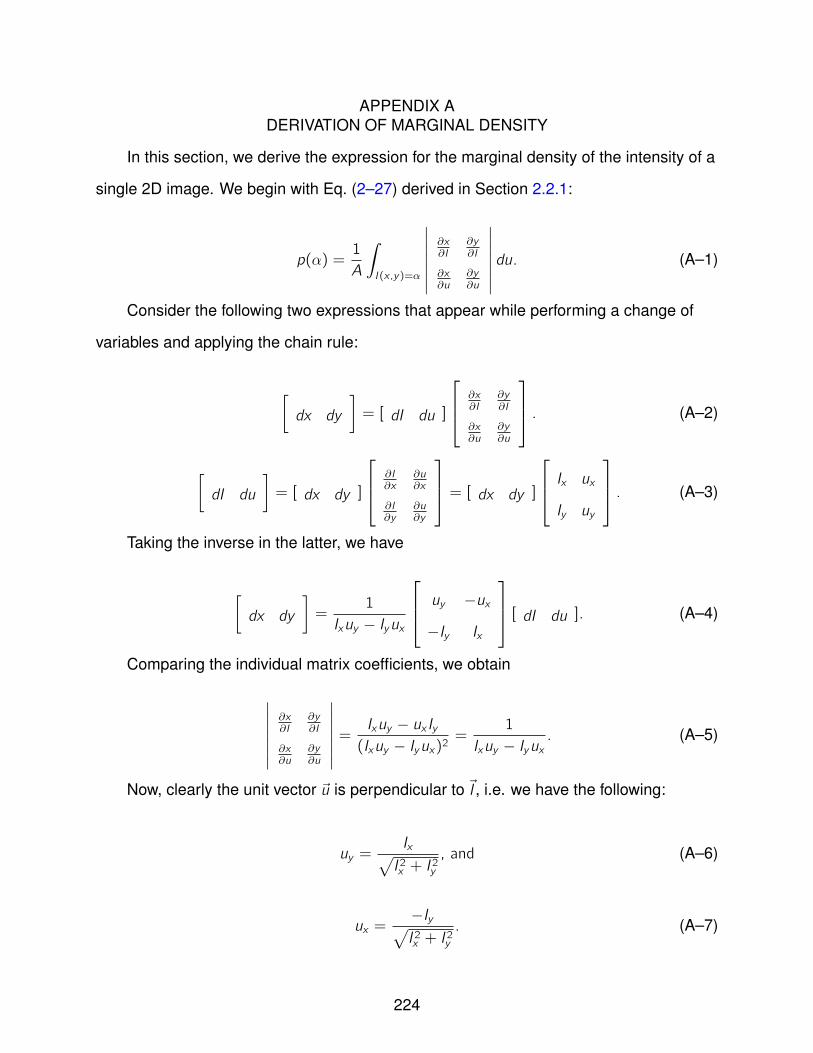
APPENDIX ADERIVATION OF MARGINAL DENSITY
In this section, we derive the expression for the marginal density of the intensity of a
single 2D image. We begin with Eq. (2–27) derived in Section 2.2.1:
p(α) =1
A
∫I (x ,y)=α
∣∣∣∣∣∣∣∂x∂I
∂y∂I
∂x∂u
∂y∂u
∣∣∣∣∣∣∣ du. (A–1)
Consider the following two expressions that appear while performing a change of
variables and applying the chain rule:
[dx dy
]= [ dI du ]
∂x∂I
∂y∂I
∂x∂u
∂y∂u
. (A–2)
[dI du
]= [ dx dy ]
∂I∂x
∂u∂x
∂I∂y
∂u∂y
= [ dx dy ] Ix uxIy uy
. (A–3)
Taking the inverse in the latter, we have
[dx dy
]=
1
Ixuy − Iyux
uy −ux
−Iy Ix
[ dI du ]. (A–4)
Comparing the individual matrix coefficients, we obtain
∣∣∣∣∣∣∣∂x∂I
∂y∂I
∂x∂u
∂y∂u
∣∣∣∣∣∣∣ =Ixuy − ux Iy(Ixuy − Iyux)2
=1
Ixuy − Iyux. (A–5)
Now, clearly the unit vector ~u is perpendicular to ~I , i.e. we have the following:
uy =Ix√I 2x + I
2y
, and (A–6)
ux =−Iy√I 2x + I
2y
. (A–7)
224

This finally gives us
∣∣∣∣∣∣∣∂x∂I
∂y∂I
∂x∂u
∂y∂u
∣∣∣∣∣∣∣ =1√I 2x + I
2y
. (A–8)
Hence we arrive at the following expression for the marginal density:
p(α) =1
A
∫I (x ,y)=α
du√I 2x + I
2y
. (A–9)
This is the same expression as in Eq. (2–28).
225
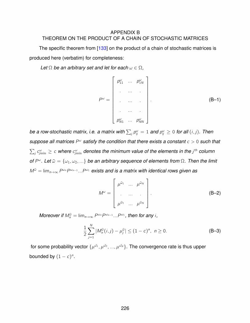
APPENDIX BTHEOREM ON THE PRODUCT OF A CHAIN OF STOCHASTIC MATRICES
The specific theorem from [133] on the product of a chain of stochastic matrices is
produced here (verbatim) for completeness:
Let Ω be an arbitrary set and let for each ω ∈ Ω,
Pω =
pω11 ... pω1N
. ... .
. ... .
. ... .
pωN1 ... pωNN
. (B–1)
be a row-stochastic matrix, i.e. a matrix with∑j p
ωij = 1 and pωij ≥ 0 for all (i , j). Then
suppose all matrices Pω satisfy the condition that there exists a constant c > 0 such that∑j c
ωjmin ≥ c where cωjmin denotes the minimum value of the elements in the j th column
of Pω. Let ω = ω1,ω2, ... be an arbitrary sequence of elements from Ω. Then the limit
M ω = limn→∞ PωnPωn−1...Pω1 exists and is a matrix with identical rows given as
Mω =
µω1 ... µωN
. ... .
µω1 ... µωN
. (B–2)
Moreover if M ωn = limn→∞ P
ωnPωn−1...Pω1, then for any i ,
1
2
N∑j=1
|M ωn (i , j)− µω
j | ≤ (1− c)n, n ≥ 0. (B–3)
for some probability vector µω1,µω2, ...,µωN. The convergence rate is thus upper
bounded by (1− c)n.
226

REFERENCES
[1] Tina Is No Acronym (TINA) Image Database, Available from http://www.tina-vision.net/ilib.php, 2008, University of Manchester and University of Sheffield, UK.
[2] A. Buades, B. Coll, and J.-M. Morel, “A review of image denoising algorithms, witha new one,” Multiscale modelling and simulation, vol. 4, no. 2, pp. 490–530, 2005.
[3] B. Silverman, Density Estimation for Statistics and Data Analysis. London, UK:Chapman and Hall, 1986.
[4] J. Simonoff, Smoothing Methods in Statistics. Berlin,Germany: Springer Verlag,1996.
[5] C. Bishop, Pattern Recognition and Machine Learning. Springer Verlag, 2006.
[6] D. Herrick, G. Nason, and B. Silverman, “Some new methods for wavelet densityestimation,” Sankhya, vol. 63, pp. 394–411, 2001.
[7] A. Peter and A. Rangarajan, “Maximum likelihood wavelet density estimation withapplications to image and shape matching,” IEEE Trans. Image Process., vol. 17,no. 4, pp. 458–468, April 2008.
[8] D. Donoho, I. Johnstone, G. Kerkyacharian, and D. Picard, “Density estimation bywavelet thresholding,” Ann. Stat., vol. 24, pp. 508–539, 1996.
[9] A. Rajwade, A. Banerjee, and A. Rangarajan, “New method of probability densityestimation with application to mutual information based image registration,”in IEEE Conf. Computer Vision and Pattern Recognition, vol. 2, 2006, pp.1769–1776.
[10] ——, “Continuous image repesentations avoid the histogram binning problemin mutual information based image registration,” in IEEE Int. Symp. BiomedicalImaging, 2006, pp. 840–843.
[11] ——, “Probability density estimation using isocontours and isosurfaces:applications to information-theoretic image registration,” IEEE Trans. PatternAnal. Mach. Intell., vol. 31, no. 3, pp. 475–491, 2009.
[12] T. Kadir and M. Brady, “Estimating statistics in arbitrary regions of interest,” inBritish Mach. Vision Conf., 2005, pp. 589–598.
[13] N. Joshi and M. Brady, “Nonparametric mixture model based evolution of levelsets,” in Int. Conf. Computing: Theory and Applications (ICCTA), 2007, pp.618–622.
[14] E. Hadjidemetriou, M. Grossberg, and S. Nayar, “Histogram preserving imagetransformations,” Int. J. Comput. Vis., vol. 45, no. 1, pp. 5–23, 2001.
227

[15] J. Boes and C. Meyer, “Multi-variate mutual information for registration,” in Med.Image Comput. Computer-Assisted Intervention, ser. LNCS, vol. 1679. Springer,1999, pp. 606–612.
[16] J. Zhang and A. Rangarajan, “Multimodality image registration using an extensibleinformation metric,” in Inf. Process. Med. Img., ser. LNCS, vol. 3565. Springer,2005, pp. 725–737.
[17] M. de Berg, M. van Kreveld, M. Overmars, and O. Schwarzkopf, ComputationalGeometry: Algorithms and Applications. Berlin, Germany: Springer Verlag, 1997.
[18] L. Rudin, S. Osher, and E. Fatemi, “Nonlinear total variation based noise removalalgorithms,” Physica D, vol. 60, pp. 259–268, 1992.
[19] D. L. Collins et al., “Design and construction of a realistic digital brain phantom,”IEEE Trans. Med. Imag., vol. 17, no. 3, pp. 463–468, 1998.
[20] J. Pluim, J. Maintz, and M. Viergever, “Mutual information based registration ofmedical images: A survey,” IEEE Trans. Med. Imag., vol. 22, no. 8, pp. 986–1004,2003.
[21] H. Chen, M. Arora, and P. Varshney, “Mutual information-based image registrationfor remote sensing data,” J. Remote Sensing, vol. 24, no. 18, pp. 3701–3706,2003.
[22] P. Viola and W. Wells, “Alignment by maximization of mutual information,” Int. J.Comput. Vis., vol. 24, no. 2, pp. 137–154, 1997.
[23] F. Maes, A. Collignon, D. Vandermeulen, G. Marchal, and P. Suetens,“Multimodality image registration by maximization of mutual information,” IEEETrans. Med. Imag., vol. 16, no. 2, pp. 187–198, 1997.
[24] F. Maes, D. Vandermeulen, and P. Suetens, “Medical image registration usingmutual information,” Proc. IEEE, vol. 91, no. 10, pp. 1699–1722, 2003.
[25] M. Rao, Y. Chen, B. Vemuri, and F. Wang, “Cumulative residual entropy: A newmeasure of information,” IEEE Trans. Inf. Theory, vol. 50, no. 6, pp. 1220–1228,2004.
[26] F. Wang and B. Vemuri, “Non-rigid multi-modal image registration usingcross-cumulative residual entropy,” Int. J. Comput. Vis., vol. 74, no. 2, pp.201–215, 2007.
[27] F. Wang, B. Vemuri, M. Rao, and Y. Chen, “Cumulative residual entropy, a newmeasure of information and its application to image alignment,” in IEEE Int. Conf.Computer Vision, 2003, pp. 548–553.
228
[28] J. Beirlant, E. Dudewicz, L. Gyorfi, and E. C. van der Meulen, “Nonparametricentropy estimation: An overview,” Int. J. Math. Stat. Sci., vol. 6, no. 1, pp. 17–39,June 1997.
[29] P. Viola, “Alignment by maximization of mutual information,” Ph.D. dissertation,Massachussets Institute of Technology, 1995.
[30] C. Yang, R. Duraiswami, N. Gumerov, and L. Davis, “Improved fast Gausstransform and efficient kernel density estimation,” in IEEE Int. Conf. ComputerVision, vol. 1, 2003, pp. 464–471.
[31] M. Leventon and W. Grimson, “Multi-modal volume registration using joint intensitydistributions,” in Med. Image Comput. Computer-Assisted Intervention, vol. 1496,1998, pp. 1057–1066.
[32] T. Downie and B. Silverman, “A wavelet mixture approach to the estimation ofimage deformation functions,” Sankhya Series B, vol. 63, pp. 181–198, 2001.
[33] B. Ma, A. Hero, J. Gorman, and O. Michel, “Image registration with minimumspanning tree algorithm,” in IEEE Int. Conf. Image Process., vol. 1, 2000, pp.481–484.
[34] J. Costa and A. Hero, “Entropic graphs for manifold learning,” in IEEE AsilomarConf. Sign., Sys. and Comp., vol. 1, 2003, pp. 316–320.
[35] M. Sabuncu and P. Ramadge, “Gradient based optimization of an EMST imageregistration function,” in IEEE Int. Conf. Acoust., Speech, Sig. Proc., vol. 2, 2005,pp. 253–256.
[36] N. Dowson, R. Bowden, and T. Kadir, “Image template matching using mutualinformation and NP-Windows,” in Int. Conf. Pattern Recognition, vol. 2, 2006, pp.1186–1191.
[37] B. Karacali, “Information theoretic deformable registration using local imageinformation,” Int. J. Comput. Vis., vol. 72, no. 3, pp. 219–237, 2007.
[38] P. Thevenaz and M. Unser, “Optimization of mutual information for multiresolutionimage registration,” IEEE Trans. Image Process., vol. 9, no. 12, pp. 2083–2099,2000.
[39] T. Cover and J. Thomas, Elements of Information Theory. New York, USA: WileyInterscience, 1991.
[40] J. Zhang and A. Rangarajan, “Affine image registration using a new informationmetric,” in IEEE Conf. Computer Vision and Pattern Recognition, vol. 1, 2004, pp.848–855.
[41] W. Feller, “On the Kolmogorov-Smirnov limit theorems for empirical distributions,”The Annals of Mathematical Statistics, vol. 19, no. 2, pp. 177–189, 1948.
229
[42] R. Shekhar and V. Zagrodsky, “Mutual information-based rigid and nonrigidregistration of ultrasound volumes,” IEEE Trans. Med. Imag., vol. 21, no. 1, pp.9–22, 2002.
[43] L. Devroye, L. Gyorfi, and G. Lugosi, A Probabilistic Theory of Pattern Recogni-tion. Berlin, Germany: Springer Verlag, 1996.
[44] P. Perona and J. Malik, “Scale-space and edge detection using anisotropicdiffusion,” IEEE Trans. Pattern Anal. Mach. Intell., vol. 12, no. 7, pp. 629–639,1990.
[45] D. Tschumperle and R. Deriche, “Vector-valued image regularization with PDEs :A common framework for different applications,” IEEE Trans. Pattern Anal. Mach.Intell., vol. 27, no. 4, pp. 506–517, 2005.
[46] B. Tang and G. Sapiro, “Color image enhancement via chromaticity diffusion,”IEEE Trans. Image Process., vol. 10, pp. 701–707, 1999.
[47] P. Saint-Marc, J. Chen, and G. Medioni, “Adaptive smoothing: a general tool forearly vision,” IEEE Trans. Pattern Anal. Mach. Intell., vol. 13, no. 6, pp. 514–520,1991.
[48] K. Plataniotis and A. Venetsanopoulos, Color image processing and applications.New York, USA: Springer Verlag, 2000.
[49] C. Tomasi and R. Manduchi, “Bilateral filtering for gray and color images,” in IEEEInt. Conf. Computer Vision, 1998, pp. 839–846.
[50] Y. Cheng, “Mean shift, mode seeking and clustering,” IEEE Trans. Pattern Anal.Mach. Intell., vol. 17, no. 8, pp. 790–799, 1995.
[51] D. Comaniciu and P. Meer, “Mean shift: a robust approach toward feature spaceanalysis,” IEEE Trans. Pattern Anal. Mach. Intell., vol. 24, no. 5, pp. 603–619,2002.
[52] A. Rajwade, A. Banerjee, and A. Rangarajan, “Image filtering driven by levelcurves,” in Int. Conf. Energy Min. Methods Computer Vision Pattern Recognition,2009, pp. 359–372.
[53] T. Chan and J. Shen, Image Processing and Analysis: Variational, PDE, wavelets,and stochastic methods. SIAM, 2005.
[54] D. Barash and D. Comaniciu, “A common framework for nonlinear diffusion,adaptive smoothing, bilateral filtering and mean shift,” Image Vis. Comput., vol. 22,pp. 73–81, 2004.
[55] A. Buades, B. Coll, and J.-M. Morel, “Neighborhood filters and PDEs,” NumerischeMathematik, vol. 105, no. 1, pp. 1–34, 2006.
230
[56] R. Subbarao and P. Meer, “Discontinuity preserving filtering over analyticmanifolds,” in IEEE Conf. Computer Vision and Pattern Recognition, 2007, pp.1–6.
[57] J. van de Weijer and R. van den Bloomgard, “Local mode filtering,” in IEEE Conf.Computer Vision and Pattern Recognition, vol. 2, 2001, pp. 428–436.
[58] N. Sochen, R. Kimmel, and R. Malladi, “A general framework for low level vision,”IEEE Trans. Image Process., vol. 7, pp. 310–318, 1998.
[59] D. Comaniciu, “An algorithm for data-driven bandwidth selection,” IEEE Trans.Pattern Anal. Mach. Intell., vol. 25, pp. 281–288, 2003.
[60] D. Comaniciu, V. Ramesh, and P. Meer, “The variable bandwidth mean shiftand data-driven scale selection,” in IEEE Int. Conf. Computer Vision, 2001, pp.438–445.
[61] D. Martin, C. Fowlkes, D. Tal, and J. Malik, “A database of human segmentednatural images and its application to evaluating segmentation algorithms andmeasuring ecological statistics,” in IEEE Int. Conf. Computer Vision, vol. 2, 2001,pp. 416–423.
[62] S. Lansel, “About DenoiseLab,” Available from http://www.stanford.edu/∼slansel/DenoiseLab/documentation.htm, 2006.
[63] Z. Wang, E. Simoncelli, and A. Bovik, “Multi-scale structural similarity for imagequality assessment,” in IEEE Asilomar Conf. Signals, Sys. Comp., 2003, pp.1398–1402.
[64] O. Subakan, J. Bing, B. Vemuri, and E. Vallejos, “Feature preserving imagesmoothing using a continuous mixture of tensors,” in IEEE Int. Conf. ComputerVision, 2007, pp. 1–6.
[65] H. Takeda, S. Farsiu, and P. Milanfar, “Kernel regression for image processing andreconstruction,” IEEE Trans. Image Process., vol. 16, no. 2, pp. 349–366, 2007.
[66] K. Mardia and P. Jupp, Directional Statistics. Chichester, UK: Wiley Interscience,2000.
[67] P. Kim and J. Koo, “Directional mixture models and optimal estimation of themixing density,” Can. J. Stat., pp. 383–398, 1998.
[68] A. Banerjee, I. Dhillon, J. Ghosh, and S. Sra, “Clustering on the unit hypersphereusing von Mises-Fisher distributions,” J. Mach. Learning Res., vol. 6, pp.1345–1382, 2005.
[69] T. McGraw, B. Vemuri, R. Yezierski, and T. Mareci, “Von Mises-Fisher mixturemodel of the diffusion ODF,” in IEEE Int. Symp. Biomedical Imaging, 2006, pp.65–68.
231
[70] A. Prati, S. Calderara, and R. Cucchiara, “Using circular statistics for trajectoryshape analysis,” in IEEE Conf. Computer Vision and Pattern Recognition, June2008, pp. 1–6.
[71] K. Hara, K. Nishino, and K. Ikeuchi, “Multiple light sources and reflectanceproperty estimation based on a mixture of spherical distributions,” IEEE Int. Conf.Computer Vision, vol. 2, pp. 1627–1634, Oct. 2005.
[72] C. Han, B. Sun, R. Ramamoorthi, and E. Grinspun, “Frequency domain normalmap filtering,” ACM Trans. Graphics, vol. 26, no. 3, pp. 28–37, 2007.
[73] O. Eugeciouglu and A. Srinivasan, “Efficient nonparametric density estimationon the sphere with applications in fluid mechanics,” SIAM Journal on ScientificComputing, vol. 22, no. 1, pp. 152–176, 2000.
[74] A. Papoulis, Probability, Random Variables and Stochastic Processes. McGrawHill, 1984.
[75] H. Schaeben, “Normal orientation distributions,” Textures and Microstructures,vol. 19, pp. 197–202, 1992.
[76] A. Bijral, M. Breitenbach, and G. Grudic, “Mixture of Watson distributions: Agenerative model for hyperspherical embeddings,” in AI and Statistics, 2007, pp.1–8.
[77] T. Downs and A. L. Gould, “Some relationships between the normal and vonMises distributions,” Biometrika, vol. 54, no. 3, pp. 684–687, 1967.
[78] B. Presnell, S. Morrison, and R. Littell, “Projected multivariate linear models fordirectional data,” J. Am. Stat. Assoc., vol. 93, no. 443, pp. 1068–1077, 1998.
[79] T. Gevers and H. Stokman, “Robust histogram construction from color invariantsfor object recognition,” IEEE Trans. Pattern Anal. Mach. Intell., vol. 25, no. 10, pp.113–118, 2003.
[80] B. Pelletier, “Kernel density estimation on Riemannian manifolds,” Stat. Prob.Letters, vol. 73, pp. 297–304, 2005.
[81] D. Donoho and T. Weissman, “Recent trends in denoising tutorial, ISIT 2007,”Available from http://www.stanford.edu/∼slansel/tutorial/summary.htm, 2007.
[82] B. M. ter Haar Romeny, Geometry-driven diffusion in computer vision. Utrecht,Netherlands: Kluwer, 1994.
[83] J. Weickert, Anisotropic Diffusion in Image Processing. Stuttgart, Germany:Teubner, 1998.
[84] M. Black, G. Sapiro, D. Marimont, and D. Heeger, “Robust anisotropic diffusion,”IEEE Trans. Image Process., vol. 7, no. 3, pp. 421–432, 1998.
232
[85] F. Catte, P. Lions, J. Morel, and T. Coll, “Image selective smoothing and edgedetection by nonlinear diffusion,” SIAM J. Numer. Anal., vol. 29, no. 1, pp.182–193, 1992.
[86] L. Rudin and S. Osher, “Total variation based image resoration with free localconstraints,” in IEEE Int. Conf. Image Process., 1994, pp. 31–35.
[87] T. Le, R. Chartrand, and T. Asaki, “A variational approach to reconstructingimages corrupted by Poisson noise,” J. Math. Imag. Vis., vol. 27, pp. 257–263,2007.
[88] G. Gilboa, N. Sochen, and Y. Zeevi, “Image enhancement and denoising bycomplex diffusion processes,” IEEE Trans. Pattern Anal. Mach. Intell., vol. 26,no. 8, pp. 1020–1036, 2004.
[89] D. Seo and B. Vemuri, “Complex diffusion on scalar and vector valued imagegraphs,” in Int. Conf. Energy Min. Methods Comput. Vision Pattern Recognition,2009, pp. 98–111.
[90] Y. You and M. Kaveh, “Fourth order partial differential equations for noise removal,”IEEE Trans. Image Process., vol. 9, no. 10, pp. 1723–1730, 2000.
[91] M. Hajiaboli, “An anisotropic fourth-order partial differential equation for noiseremoval,” in Scale Space and Variational Methods in Computer Vision, 2009, pp.356–367.
[92] P. Mrazek, “Monotonicity enhancing nonlinear diffusion,” J. Visual Commun. ImageRepresentation, vol. 13, no. 1, pp. 313–323, 2000.
[93] A. Savitzky and M. Golay, “Smoothing and differentiation of data by simplified leastsquares procedures,” Anal. Chem., vol. 36, no. 8, pp. 1627–1639, 1964.
[94] W. Press, A. Teukolsky, W. Vetterling, and B. Flannery, Numerical recipes in C(2nd ed.): the art of scientific computing. New York, NY, USA: CambridgeUniversity Press, 1992.
[95] J. Fan and I. Gijbels, Local polynomial modeling and its application. London, UK:Chapman and Hill, 1996.
[96] S. M. Smith and J. M. Brady, “SUSAN - a new approach to low level imageprocessing,” Int. J. Comput. Vis., vol. 23, pp. 45–78, 1995.
[97] V. Katkovnik, A. Foi, K. Egiazarian, and J. Astola, “Directional varying scaleapproximations for anisotropic signal processing,” in Eur. Signal Process. Conf.,2004, pp. 1–6.
[98] K. Fukunaga and L. Hostetler, “The estimation of the gradient of a densityfunction, with applications in pattern recognition,” IEEE Trans. Inf. Theory, vol. 21,no. 1, pp. 32–40, 1975.
233

[99] M. Elad, “On the origin of the bilateral filter and ways to improve it,” IEEE Trans.Image Process., vol. 11, no. 10, pp. 1141–1151, 2002.
[100] N. Sochen, R. Kimmel, and A. Bruckstein, “Diffusions and confusions in signal andimage processing,” J. Math. Imag. Vis., vol. 14, pp. 195–209, 2001.
[101] O. Subakan, “Continuous mixture models for feature preserving smoothing andsegmentation,” Ph.D. dissertation, University of Florida, 2009.
[102] B. Jian, B. Vemuri, E. Ozarslan, P. Carney, and T. Mareci, “A novel tensordistribution model for the diffusion-weighted MR signal,” Neuroimage, vol. 37,no. 1, pp. 164–176, 2007.
[103] D. Tschumperle, “Fast anisotropic smoothing of multi-valued images usingcurvature-preserving PDEs,” Int. J. Comput. Vis., vol. 68, no. 1, pp. 65–82, 2006.
[104] R. Frankot and R. Chellappa, “A method for enforcing integrability in shape fromshading algorithms,” IEEE Trans. Pattern Anal. Mach. Intell., vol. 10, no. 4, pp.439–451, 1988.
[105] A. Agrawal and R. Raskar, “Short course (ICCV 2007): Gradient domainmanipulation techniques in vision and graphics,” http://www.umiacs.umd.edu/∼aagrawal/ICCV2007Course/index.html, 2007.
[106] H. Wang, Y. Chen, T. Fang, J. Tyan, and N. Ahuja, “Gradient adaptive imagerestoration and enhancement,” in Int. Conf. Image Proc., 2006, pp. 2893–2896.
[107] P. Hancock, R. Baddeley, and L. Smith, “The principal components of naturalimages,” Network: Computation in Neural Systems, vol. 3, pp. 61–72, 1992.
[108] R. Coifman and D. Donoho, “Translation-invariant denoising,” Yale University, Tech.Rep., 1995.
[109] L. Yaroslavsky, K. Egiazarian, and J. Astola, “Transform domain image restorationmethods: review, comparison and interpretation,” in SPIE Proceedings Series,Nonlinear Processing and Pattern Analysis, 2001, pp. 1–15.
[110] W. Freeman and E. Adelson, “The design and use of steerable filters,” IEEE Trans.Pattern Anal. Mach. Intell., vol. 13, no. 9, pp. 891–906, 1991.
[111] J.-L. Starck, E. Candes, and D. Donoho, “The curvelet transform for imagedenoising,” IEEE Trans. Image Process., vol. 11, no. 6, pp. 670–684, 2002.
[112] J. Fan and R. Li, “Variable selection via nonconcave penalized likelihood and itsoracle properties,” J. Am. Stat. Assoc., vol. 96, no. 456, pp. 1348–1360, December2001.
[113] D. Donoho and I. Johnstone, “Ideal spatial adaptation by wavelet shrinkage,”Biometrika, vol. 81, pp. 425–455, 1993.
234
[114] J. Mairal, G. Sapiro, and M. Elad, “Learning multiscale sparse representations forimage and video restoration,” Multiscale Modeling and Simulation, vol. 7, no. 1, pp.214–241, 2008.
[115] L. Sendur and I. Selesnick, “Bivariate shrinkage functions for wavelet-baseddenoising exploiting interscale dependency,” IEEE Trans. Signal Process., vol. 50,no. 11, pp. 2744–2756, 2002.
[116] E. Simoncelli, “Bayesian denoising of visual images in the wavelet domain,” inLecture Notes in Statistics, vol. 141, 1999, pp. 291–308.
[117] J. Portilla, V. Strela, M. Wainwright, and E. Simoncelli, “Image denoising usingscale mixtures of Gaussians in the wavelet domain,” IEEE Trans. Image Process.,vol. 12, no. 11, pp. 1338–1351, 2003.
[118] A. Hyvarinen, P. Hoyer, and E. Oja, “Image denoising by sparse code shrinkage,”in Intelligent Signal Processing, 1999, pp. 1–6.
[119] J. Huang and D. Mumford, “Statistics of natural images and models,” IEEE Conf.Computer Vision and Pattern Recognition, vol. 1, pp. 1541–1548, 1999.
[120] Y. Hel-Or and D. Shaked, “A discriminative approach for wavelet denoising,” IEEETrans. Image Process., vol. 17, no. 4, pp. 443–457, 2008.
[121] A. Buades, B. Coll, and J.-M. Morel, “Nonlocal image and movie denoising,” Int. J.Comput. Vis., vol. 76, no. 2, pp. 123–139, 2008.
[122] T. Brox, O. Kleinschmidt, and D. Cremers, “Efficient nonlocal means for denoisingof textural patterns,” IEEE Trans. Image Process., vol. 17, no. 7, pp. 1083–1092,2008.
[123] M. Ghazel, G. Freeman, and E. Vrscay, “Fractal image denoising,” IEEE Trans.Image Process., vol. 12, no. 12, pp. 1560–1578, 2003.
[124] S. Awate and R. Whitaker, “Unsupervised, information-theoretic, adaptive imagefiltering for image restoration,” IEEE Trans. Pattern Anal. Mach. Intell., vol. 28,no. 3, pp. 364–376, 2006.
[125] K. Popat and R. Picard, “Cluster-based probability model and its application toimage and texture processing,” IEEE Trans. Image Process., vol. 6, no. 2, pp.268–284, 1997.
[126] A. Efros and T. Leung, “Texture synthesis by nonparametric sampling,” in IEEE Int.Conf. Computer Vision, 1999, pp. 1033–1038.
[127] J. D. Bonet, “Noise reduction through detection of signal redundancy,” MIT, AI Lab,Tech. Rep., 1997.
235

[128] D. Zhang and Z. Wang, “Restoration of impulse noise corrupted images usinglong-range correlation,” IEEE Signal Process. Letters, vol. 5, no. 1, pp. 4–6, 1998.
[129] ——, “Image information restoration based on long-range correlation,” IEEE Trans.Circuit Syst. Video Technol., vol. 12, no. 5, pp. 331–341, 2002.
[130] S. Kindermann, S. Osher, and P. Jones, “Deblurring and denoising of images bynonlocal functionals,” SIAM Interdisc. J., vol. 4, no. 4, pp. 1091–1115, 2005.
[131] M. Ebrahimi and E. Vrscay, “Self-similarity in imaging, 20 years after ‘fractalseverywhere’,” in Int. Workshop Local Non-Local Approx. Image Process., 2008,pp. 165–172.
[132] O. Kleinschmidt, T. Brox, and D. Cremers, “Nonlocal texture filtering with efficienttree structures and invariant patch similarity measures,” in Int. Workshop LocalNon-Local Approx. Image Process., 2008, pp. 1–8.
[133] O. Stenflo, “Perfect sampling from the limit of deterministic products of stochasticmatrices,” Electronic Commun. Prob., vol. 13, pp. 474–481, 2008.
[134] K. Dabov, A. Foi, V. Katkovnik, and K. Egiazarian, “Image denoising by sparse3-d transform-domain collaborative filtering,” IEEE Trans. Image Process., vol. 16,no. 8, pp. 2080–2095, 2007.
[135] K. Hirakawa and T. Parks, “Image denoising using total least squares,” IEEETrans. Image Process., vol. 15, no. 9, pp. 2730–2742, 2006.
[136] L. Dascal, M. Zibulevsky, and R. Kimmel, “Signal denoising by constraining theresidual to be statistically noise-similar,” Technion, Israel, Tech. Rep., 2008.
[137] E. Tadmor, S. Nezzar, and L. Vese, “A multiscale image representation usinghierarchical (BV,L2) decompositions,” Multiscale modelling and simulation, vol. 2,pp. 554–579, 2004.
[138] S. Osher, M. Burger, D. Goldfarb, J. Xu, and W. Yin, “An iterative regularizationmethod for total variation-based image restoration,” Multiscale modelling andsimulation, vol. 4, pp. 460–489, 2005.
[139] J. Polzehl and V. Spokoiny, “Image denoising: a pointwise adaptive approach,”Ann. Stat., vol. 31, no. 1, pp. 30–57, 2003.
[140] J. Kleinberg and E. Tardos, Algorithm Design. Boston, USA: Addison-WesleyLongman, 2005.
[141] D. Brunet, E. Vrscay, and Z. Wang, “The use of residuals in image denoising,” inInt. Conf. Image Anal. Recognition, 2009, pp. 1–12.
236
[142] Y. Chen, H. Wang, T. Fang, and J. Tyan, “Mutual information regularized bayesianframework for multiple image restoration,” in IEEE Int. Conf. Computer Vision,2005, pp. 190–197.
[143] B. Olshausen and D. Field, “Emergence of simple-cell receptive-field properties bylearning a sparse code for natural images,” Nature, vol. 381, no. 6583, p. 607609,1996.
[144] M. Lewicki, T. Sejnowski, and H. Hughes, “Learning overcompleterepresentations,” Neural Computation, vol. 12, pp. 337–365, 1998.
[145] M. Lewicki and B. Olshausen, “A probabilistic framework for the adaptation andcomparison of image codes,” J. Opt. Soc. Am., vol. 16, pp. 1587–1601, 1999.
[146] M. Elad and M. Aharon, “Image denoising via learned dictionaries and sparserepresentation,” in IEEE Conf. Computer Vision and Pattern Recognition, vol. 1,2006, pp. 17–22.
[147] M. Aharon, M. Elad, and A. Bruckstein, “The K-SVD: an algorithm for designing ofovercomplete dictionaries for sparse representation,” IEEE Trans. Signal Process.,vol. 54, no. 11, pp. 4311–4322, 2006.
[148] P. Chatterjee and P. Milanfar, “Clustering-based denoising with locally learneddictionaries,” IEEE Trans. Image Process., vol. 18, no. 7, pp. 1438–1451, 2009.
[149] J. Yang, J. Wright, T. Huang, and Y. Ma, “Image super-resolution as sparserepresentation of raw image patches,” in IEEE Int. Conf. Comp. Vis. Pattern Rec.,2008, pp. 1–8.
[150] Z. Wang and A. Bovik, “Mean squared error: Love it or leave it? A new look atsignal fidelity measures,” IEEE Signal Process. Mag., vol. 26, no. 1, pp. 98–117,2009.
[151] Z. Wang, A. Bovik, H. Sheikh, and E. Simoncelli, “Image quality assessment:From error visibility to structural similarity,” IEEE Trans. Image Process., vol. 13,no. 4, pp. 600–612, 2004.
[152] H. Andrews and C. Patterson, “Singular value decompositions and digital imageprocessing,” IEEE Trans. Acoust., Speech and Signal Process., vol. 24, no. 1, pp.425–432, 1976.
[153] ——, “Singular value decomposition (SVD) image coding,” IEEE Trans. Commun.,vol. 24, no. 4, pp. 425–432, 1976.
[154] L. Trefethen and D. Bau, Numerical Linear Algebra. SIAM: Society for Industrialand Applied Mathematics, 1997.
[155] A. Rangarajan, “Learning matrix space image representations,” in Int. Conf.Energy Min. Methods Computer Vision Pattern Recognition, 2001, pp. 153–168.
237
[156] D. Tschumperle and R. Deriche, “Orthonormal vector sets regularization withPDEs and applications,” Int. J. Comput. Vis., vol. 50, pp. 237–252, 2002.
[157] J. Ye, “Generalized low rank approximations of matrices,” Mach. Learning, vol. 61,no. 1, pp. 167–191, 2005.
[158] C. Ding and J. Ye, “Two-dimensional singular value decomposition (2DSVD) for 2Dmaps and images,” in SIAM Int. Conf. Data Mining, 2005, pp. 32–43.
[159] N. Kwak, “Principal component analysis based on L1-norm maximization,” IEEETrans. Pattern Anal. Mach. Intell., vol. 30, no. 9, pp. 1672–1680, 2008.
[160] G. Heo, P. Gader, and H. Frigui, “RKF-PCA: Robust kernel fuzzy PCA,” NeuralNetworks, vol. 22, no. 5-6, pp. 642–650, 2009.
[161] A. Efros and W. Freeman, “Image quilting for texture synthesis and transfer,” inSIGGRAPH: Annual Conf. Computer graphics and interactive techniques, 2001,pp. 341–346.
[162] A. Hyvarinen, J. Hurri, and P. Hoyer, Natural Image Statistics: A ProbabilisticApproach to Early Computational Vision. Springer, Heidelberg, 2009.
[163] A. Rosenfeld and A. Kak, Digital Picture Processing. Orlando, USA: AcademicPress, 1982.
[164] L. Tucker, “Some mathematical notes on three-mode factor analysis,” Psychome-trika, vol. 31, no. 3, pp. 279–311, 1966.
[165] L. de Lathauwer, “Signal processing based on multilinear algebra,” Ph.D.dissertation, Katholieke Universiteit Leuven, Belgium, 1997.
[166] M. Vasilescu and D. Terzopoulos, “Multilinear analysis of image ensembles:Tensorfaces,” in Int. Conf. Pattern Recognition, 2002, pp. 511–514.
[167] K. Gurumoorthy, A. Rajwade, A. Banerjee, and A. Rangarajan, “Beyond SVD:Sparse projections onto exemplar orthonormal bases for compact imagerepresentation,” in Int. Conf. Pattern Recognition, 2008, pp. 1–4.
[168] ——, “A method for compact image representation using sparse matrix and tensorprojections onto exemplar orthonormal bases,” IEEE Trans. Image Process.,vol. 19, no. 2, pp. 322–334, 2010.
[169] D. Muresan and T. Parks, “Adaptive principal components and image denoising,”in IEEE Int. Conf. Image Process., 2003, pp. 101–104.
[170] A. Rajwade, A. Rangarajan, and A. Banerjee, “Automated filter parameterselection using measures of noiseness,” in Can. Conf. Comput. Robot Vision,2010, pp. 86–93.
238

[171] J. Weickert, “Coherence enhancing diffusion filtering,” Int. J. Comput. Vis., vol. 31,no. 3, pp. 111–127, 1999.
[172] P. Mrazek and M. Navara, “Selection of optimal stopping time for nonlineardiffusion filtering,” Int. J. Comput. Vision, vol. 52, no. 2-3, pp. 189–203, 2003.
[173] J.-F. Aujol, G. Gilboa, T. Chan, and S. Osher, “Structure-texture imagedecomposition–modeling, algorithms and parameter selection,” Int. J. Comput.Vis., vol. 67, no. 1, pp. 111–136, 2006.
[174] G. Gilboa, N. Sochen, and Y. Zeevi, “Estimation of optimal PDE-based denoisingin the SNR sense,” IEEE Trans. Image Process., vol. 15, no. 8, pp. 2269–2280,Aug. 2006.
[175] I. Vanhamel, C. Mihai, H. Sahli, A. Katartzis, and I. Pratikakis, “Scale selection forcompact scale-space representation of vector-valued images,” Int. J. Comput. Vis.,vol. 84, no. 2, pp. 194–204, 2009.
[176] D. Donoho and I. Johnstone, “Adapting to unknown smoothness via waveletshrinkage,” J. Am. Stat. Assoc., vol. 90, no. 432, pp. 1200–1224, 1995.
[177] A. Dvoretzky, J. Kiefer, and J. Wolfowitz, “Asymptotic minimax character of thesample distribution function and of the classical multinomial estimator,” Ann. Math.Stat., vol. 27, no. 3, pp. 642–669, 1956.
[178] Wikipedia, “Dvoretzky Kiefer Wolfowitz inequality,” Available from http://en.wikipedia.org/wiki/Dvoretzky-Kiefer-Wolfowitz inequality, 2010.
[179] J. Kiefer, “K-sample analogues of the Kolmogorov-Smirnov and Cramer-VonMises tests,” Ann. Math. Stat., vol. 30, no. 2, pp. 420–447, 1959.
[180] F. Anscombe, “The transformation of Poisson, binomial and negative-binomialdata,” Biometrika, vol. 35, pp. 246–254, 1948.
[181] D. Donoho, “Denoising by soft thresholding,” IEEE Trans. Inf. Theory, vol. 41,no. 3, pp. 613–627, 1995.
[182] A. D. Stefano, P. White, and W. Collis, “Training methods for image noise levelestimation on wavelet components,” EURASIP J. Appl. Signal Process., vol. 2004,no. 16, pp. 2400–2407, 2004.
[183] X. Zhu and P. Milanfar, “A no-reference image content metric and its application todenoising,” in IEEE Int. Conf. Image Process., 2010, pp. 1–4.
[184] C. Boncelet, “Image noise models,” in Handbook of Image and Video Processing,A. Bovik, Ed. New York, USA: Academic Press, 2005, pp. 397–410.
239

BIOGRAPHICAL SKETCH
Ajit Rajwade was born and brought up in the city of Pune, India. He completed
his bachelor’s degree in computer engineering from the Government College of
Engineering, Pune (affiliated to the University of Pune) in 2001, his master’s degree
in computer science from McGill University, Montreal, Canada in 2004, and his doctoral
degree in computer engineering from the University of Florida in 2010. His research
interests are in computer vision and image processing, and computational geometry.
240