c© 2010 Robert De Moss Gregg IV

GEOMETRIC CONTROL AND MOTION PLANNINGFOR THREE-DIMENSIONAL BIPEDAL LOCOMOTION

BY

ROBERT DE MOSS GREGG IV

DISSERTATION

Submitted in partial fulfillment of the requirementsfor the degree of Doctor of Philosophy in Electrical and Computer Engineering

in the Graduate College of theUniversity of Illinois at Urbana-Champaign, 2010

Urbana, Illinois

Doctoral Committee:

Professor Mark W. Spong, ChairAssistant Professor Timothy W. BretlProfessor Seth A. HutchinsonAssociate Professor Daniel M. LiberzonAssistant Professor Prashant G. Mehta

ABSTRACT

This thesis presents a hierarchical geometric control approach for fast and energetically efficient

bipedal dynamic walking in three-dimensional (3-D) space to enable motion planning applications

that have previously been limited to inefficient quasi-static walkers. In order to produce exponen-

tially stable hybrid limit cycles, we exploit system energetics, symmetry, and passivity through the

energy-shaping method of controlled geometric reduction. This decouples a subsystem correspond-

ing to a lower-dimensional robot through a passivity-based feedback transformation of the system

Lagrangian into a special form of controlled Lagrangian with broken symmetry, which corresponds

to an equivalent closed-loop Hamiltonian system with upper-triangular form. The first control

term reduces to mechanically-realizable passive feedback that establishes a functional momentum

conservation law that controls the “divided” cyclic variables to set-points or periodic orbits. We

then prove extensive symmetries in the class of open kinematic chains to present the multistage

application of controlled reduction. A reduction-based control law is derived to construct straight-

ahead and turning gaits for a 4-DOF and 5-DOF hipped biped in 3-D space, based on the existence

of stable hybrid limit cycles in the sagittal plane-of-motion. Given such a set of asymptotically

stable gait primitives, a dynamic walker can be controlled as a discrete-time switched system that

sequentially composes gait primitives from step to step. We derive “funneling” rules by which a

walking path that is a sequence of these gaits may be stably followed by the robot. The primitive

set generates a tree exploring the action space for feasible walking paths, where each primitive

corresponds to walking along a nominal arc of constant curvature. Therefore, dynamically stable

motion planning for dynamic walkers reduces to a discrete search problem, which we demonstrate

for 3-D compass-gait bipeds. After reflecting on several connections to human biomechanics, we

propose extensions of this energy-shaping control paradigm to robot-assisted locomotor therapies.

ii

To my parents, Robert D. Gregg III and Leslie A. Gregg, for their love and support

iii

ACKNOWLEDGMENTS

I am forever grateful for my experiences at the Coordinated Science Laboratory (CSL) and Depart-

ment of Electrical and Computer Engineering at the University of Illinois at Urbana-Champaign.

I would first like to thank my adviser, Mark W. Spong, for his unwavering support, advice, and

encouragement in my research pursuits over the past four years. During both his time at CSL and

more recently at the University of Texas at Dallas, he offered me the perfect balance of guidance

and autonomy that effectively taught me to be a controls researcher. I am very fortunate to have

had the opportunity to work with him.

I would also like to thank the other members of my committee, Timothy W. Bretl, Seth Hutchin-

son, Daniel Liberzon, and Prashant G. Mehta, who served as a network of support and inspiration

at CSL. In particular, Prashant Mehta challenged me to understand the symmetry and symmetry-

breaking aspects of controlled geometric reduction. The multiple courses I took with him and

Daniel Liberzon contributed greatly to my understanding of control theory. I enjoyed the motivat-

ing and sometimes philosophical conversations with Tim Bretl, who pushed me to see connections

to motion planning and human rehabilitation during the later years of my studies. He and Seth

Hutchinson kindly welcomed me to their research group meetings after my adviser’s departure to

UT Dallas, which encouraged collaborations and ideas that I might otherwise have missed.

Of course, many other members of the Decision and Control group at CSL deserve recognition.

Dusan Stipanovic welcomed me to CSL with friendly conversations and reflections on our experi-

ences in California’s Bay Area. Sean Meyn and Todd Coleman offered endless encouragement in

my pursuit of various research topics and ultimately post-doctoral positions. Several Ph.D. candi-

dates provided invaluable mentoring during my early years as a graduate student. For this, I am

indebted to Peter Hokayem, Silvia Mastellone, Jonathan Holm, Shankar Rao, and Shreyas Sun-

daram. I might not have weathered the adjustment to Urbana-Champaign and academia at large

were it not for them. The support staff of the Decision and Control group, Ronda Rigdon, Becky

iv

Lonberger, and Jana Lenz, deserve great thanks. Their warm conversations and administrative

expertise made my time at CSL all the more memorable. I would also like to thank Robert Mc-

Cabe and Nikolaos Freris for the late conversations at CSL and for refreshing my less-than-perfect

memory on real analysis. Recognition is due to my undergraduate assistant, Adam Tilton, for

his outstanding work on the planned walking simulations in this thesis. The project reached this

higher level thanks to his programming contributions and the helpful advice of Sal Candido.

My colleagues and friends around CSL and the University made all the difference in my experience

at the University of Illinois. To name a few not already mentioned: Nikhil Chopra, Aneel Tanwani,

Yoav Sharon, Stephan Trenn, Dayu Huang, Neera Jain, Kira Barton, Alex Shorter, David Hoelzle,

Miles Johnson, Jeremy Kemmerer, Ashlee Ford, Erick Rodriguez-Seda, Jae-Sung Moon, Adam

Cushman, Melody Bonham, Shreyas Prasad, Jeff Lee, Nitin Navale, Bill Eisenhower, Greg Lucas,

Roger Serwy, Sundeep Kartan, Mike King, Scott Jobling, Megan Haselschwerdt, Patrick Lynch,

Lance Kingston, and Carey Ash. I also greatly enjoyed the many ice hockey seasons with CSL

colleagues Spencer Brady, Jared McNew, and John Sartori.

I would like to recognize Jessy W. Grizzle, Ambarish Goswami, and Romeo Ortega for their many

helpful comments on my papers and the inspiration they provided through their own work. I also

thank Aaron D. Ames and S. Shankar Sastry for advising and training me as an undergraduate

researcher during my time at the University of California, Berkeley. Our work served as the

foundation for this thesis project. My fellow student and friend at UC Berkeley, Eric D.B. Wendel,

also deserves recognition for coding the early version of our Matlab simulation package.

I am most grateful for the support of my family in California, Rob, Leslie, and Joseph Gregg; my

surrogate family in Urbana-Champaign, Joe, Bea, and Nick Pavia; and my loving partner Kristin

Drogos. They have stood by me through the good times and the very difficult times. Wayne and

Kay Carter mentored me from my childhood, and to this day provide a source of inspiration and

pride. I also enjoyed the company of my dog, Oskee, while writing this thesis.

In closing, I kindly thank my many colleagues in the IFAC American Automatic Control Council

for the unexpected support and motivation they provided for this line of work. The past four

years of research would not have been possible without the financial support of National Science

Foundation grants CMS-0510119 and CMMI-0856368.

v

TABLE OF CONTENTS

LIST OF ABBREVIATIONS . . . . . . . . . . . . . . . . . . . . . . . . . . . . . . . . . . . . viii

LIST OF SYMBOLS . . . . . . . . . . . . . . . . . . . . . . . . . . . . . . . . . . . . . . . . . x

CHAPTER 1 INTRODUCTION . . . . . . . . . . . . . . . . . . . . . . . . . . . . . . . . . 11.1 Hybrid Systems . . . . . . . . . . . . . . . . . . . . . . . . . . . . . . . . . . . . . . . 11.2 Quasi-Static Walking . . . . . . . . . . . . . . . . . . . . . . . . . . . . . . . . . . . . 41.3 Dynamic Walking . . . . . . . . . . . . . . . . . . . . . . . . . . . . . . . . . . . . . . 51.4 Contributions of the Thesis . . . . . . . . . . . . . . . . . . . . . . . . . . . . . . . . 81.5 Organization of the Thesis . . . . . . . . . . . . . . . . . . . . . . . . . . . . . . . . . 11

CHAPTER 2 PASSIVITY AND SYMMETRY IN MECHANICAL SYSTEMS . . . . . . . 122.1 Lagrangian Mechanics . . . . . . . . . . . . . . . . . . . . . . . . . . . . . . . . . . . 132.2 Hamiltonian Mechanics . . . . . . . . . . . . . . . . . . . . . . . . . . . . . . . . . . 142.3 Passivity . . . . . . . . . . . . . . . . . . . . . . . . . . . . . . . . . . . . . . . . . . . 152.4 Symmetry . . . . . . . . . . . . . . . . . . . . . . . . . . . . . . . . . . . . . . . . . . 172.5 Geometric Reduction . . . . . . . . . . . . . . . . . . . . . . . . . . . . . . . . . . . . 19

CHAPTER 3 CONTROLLED GEOMETRIC REDUCTION . . . . . . . . . . . . . . . . . 213.1 Control of Cyclic Variables . . . . . . . . . . . . . . . . . . . . . . . . . . . . . . . . 223.2 Almost-Cyclic Lagrangians . . . . . . . . . . . . . . . . . . . . . . . . . . . . . . . . 313.3 Reduced Subsystem . . . . . . . . . . . . . . . . . . . . . . . . . . . . . . . . . . . . 343.4 Almost-Cyclic Hamiltonians . . . . . . . . . . . . . . . . . . . . . . . . . . . . . . . . 36

CHAPTER 4 REDUCTION-BASED CONTROL OF MECHANICAL SYSTEMS . . . . . . 414.1 Symmetries in Serial Kinematic Chains . . . . . . . . . . . . . . . . . . . . . . . . . 424.2 Symmetries in Branched Kinematic Chains . . . . . . . . . . . . . . . . . . . . . . . 434.3 Controlled Reduction by Stages . . . . . . . . . . . . . . . . . . . . . . . . . . . . . . 464.4 Attractivity of the Zero Dynamics . . . . . . . . . . . . . . . . . . . . . . . . . . . . 51

CHAPTER 5 THREE-DIMENSIONAL BIPEDAL WALKING . . . . . . . . . . . . . . . . 535.1 Bipedal Walking Robots . . . . . . . . . . . . . . . . . . . . . . . . . . . . . . . . . . 535.2 Reduction-Based Control Law . . . . . . . . . . . . . . . . . . . . . . . . . . . . . . . 595.3 Four-DOF Biped Simulations . . . . . . . . . . . . . . . . . . . . . . . . . . . . . . . 645.4 Five-DOF Biped Simulations . . . . . . . . . . . . . . . . . . . . . . . . . . . . . . . 725.5 Energetic Efficiency . . . . . . . . . . . . . . . . . . . . . . . . . . . . . . . . . . . . 765.6 Remarks . . . . . . . . . . . . . . . . . . . . . . . . . . . . . . . . . . . . . . . . . . . 78

vi

CHAPTER 6 GAIT PRIMITIVES FOR MOTION PLANNING . . . . . . . . . . . . . . . 806.1 Quasi-Static Motion Planning . . . . . . . . . . . . . . . . . . . . . . . . . . . . . . . 806.2 Asymptotically Stable Gait Primitives . . . . . . . . . . . . . . . . . . . . . . . . . . 816.3 Sequential Composition of Gait Primitives . . . . . . . . . . . . . . . . . . . . . . . . 826.4 Path Planning Formulation . . . . . . . . . . . . . . . . . . . . . . . . . . . . . . . . 856.5 Primitives for 3-D Compass-Gait Bipeds . . . . . . . . . . . . . . . . . . . . . . . . . 876.6 Planned Walking Results . . . . . . . . . . . . . . . . . . . . . . . . . . . . . . . . . 976.7 Remarks . . . . . . . . . . . . . . . . . . . . . . . . . . . . . . . . . . . . . . . . . . . 100

CHAPTER 7 EXTENSIONS TO LOCOMOTOR REHABILITATION . . . . . . . . . . . . 1027.1 Connections to Human Biomechanics . . . . . . . . . . . . . . . . . . . . . . . . . . . 1027.2 Challenges in Robot-Assisted Therapy . . . . . . . . . . . . . . . . . . . . . . . . . . 1057.3 Control Design Methodology . . . . . . . . . . . . . . . . . . . . . . . . . . . . . . . 1067.4 Potential Impact . . . . . . . . . . . . . . . . . . . . . . . . . . . . . . . . . . . . . . 108

CHAPTER 8 CONCLUSIONS . . . . . . . . . . . . . . . . . . . . . . . . . . . . . . . . . . 1098.1 Autonomous Robot Walking . . . . . . . . . . . . . . . . . . . . . . . . . . . . . . . . 1108.2 Robot-Assisted Locomotor Rehabilitation . . . . . . . . . . . . . . . . . . . . . . . . 111

APPENDIX A PROPERTIES OF ALMOST-CYCLIC LAGRANGIAN SYSTEMS . . . . . 112A.1 Inertia Matrix . . . . . . . . . . . . . . . . . . . . . . . . . . . . . . . . . . . . . . . . 112A.2 Skew-Symmetry . . . . . . . . . . . . . . . . . . . . . . . . . . . . . . . . . . . . . . . 113

APPENDIX B PROOF OF CONTROLLED REDUCTION THEOREM . . . . . . . . . . . 116

APPENDIX C BIPED INERTIA MATRIX TERMS . . . . . . . . . . . . . . . . . . . . . . 120C.1 4-DOF Hipped Biped . . . . . . . . . . . . . . . . . . . . . . . . . . . . . . . . . . . 120C.2 5-DOF Hipped Biped . . . . . . . . . . . . . . . . . . . . . . . . . . . . . . . . . . . 121

REFERENCES . . . . . . . . . . . . . . . . . . . . . . . . . . . . . . . . . . . . . . . . . . . . 125

AUTHOR’S BIOGRAPHY . . . . . . . . . . . . . . . . . . . . . . . . . . . . . . . . . . . . . 134

vii

LIST OF ABBREVIATIONS

ZMP Zero moment point.

CoP Center of pressure.

FRI Foot rotation indicator.

IDA Interconnection and damping assignment.

RLC Resistor/capacitor/inductor.

2-D Two-dimensional space (planar).

3-D Three-dimensional space.

DOF Degree(s) of freedom.

4D 4-DOF biped.

5D 5-DOF biped.

A Assumption.

E-L Euler-Lagrange.

AS Asymptotically stable.

GAS Globally asymptotically stable.

ES Exponentially stable.

LES Locally exponentially stable.

GES Globally exponentially stable.

CICS Convergent-input convergent-state.

BoA Basin of attraction.

LTI Linear time-invariant.

LTV Linear time-varying.

PD Proportional-derivative.

viii

ACH Almost-cyclic Hamiltonian.

ACL Almost-cyclic Lagrangian.

k-ACL k-almost-cyclic Lagrangian.

GRF Ground reaction force(s).

CW Clockwise.

CCW Counter-clockwise.

S Straight.

LQR Linear quadratic regulator.

CoM Center of mass.

EMG Electromyography.

RoM Range of motion.

AFO Ankle-foot orthosis.

ix

LIST OF SYMBOLS

∇ Gradient operator, i.e., vectorized partial derivative operator.

L Lie derivative operator, i.e., change of a function along the flow of a vector field.

K Kinetic energy.

V Potential energy.

H Hamiltonian function, i.e., total energy.

L Lagrangian function.

R Routhian function.

M Inertia/mass matrix.

C Coriolis matrix.

Q Gyroscopic matrix.

N Potential torque vector.

B Control input to torque map.

u Control input.

v Auxiliary control input.

f Vector field.

g Control input vector fields.

H C Hybrid control system.

H Hybrid system.

P Poincare map.

∆ Impact map.

G Guard/switching surface.

O Periodic orbit.

x

J Momentum map.

Jc Constraint Jacobian.

J Optimality performance index.

SO(n) Special orthogonal group of dimension n.

SE(n) Special Euclidean group of dimension n.

S1 Unit circle group.

Rn n-dimensional real numbers group.

Tn n-dimensional torus group.

Q Configuration space.

S Shape space, i.e., reduced configuration space.

G Symmetry group.

TQ Tangent bundle of Q, i.e., the phase space.

T ∗Q Cotangent bundle of Q, i.e., the phase space.

TS Tangent bundle of S, i.e., the reduced phase space.

Z Invariant surface in TQ.

D Invariant surface in T ∗S1.

q Generalized configuration vector.

p Generalized momentum vector.

x Phase state vector, i.e., (q, q) ∈ TQ.

λ Conserved momentum function.

ψ Biped yaw (heading) angle.

ϕ Biped roll (lean) angle.

θs Biped stance pitch angle.

θt Biped torso pitch angle.

θns Biped nonstance (swing) pitch angle.

s Step cycle steering angle.

G Asymptotically stable gait primitive.

P Set of asymptotically stable gait primitives.

T Gait transition.

E Walking path execution.

S Sequence of steering angles (output of planner).

xi

CHAPTER 1

INTRODUCTION

The step-level control and high-level motion planning of humanoid walking have been active ar-

eas of research over the past decades. Robotic technology is proving essential to alleviating the

intensive labor required by physical therapists in locomotor rehabilitation, restoring mobility in

lower-extremity amputees with powered prosthesis, and providing gait assistance to the disabled

or elderly. The incredible efficiency of bipedalism, which allows humans to outwalk quadrupeds

over long distances [1, 2], also motivates its use on autonomous locomotive mechanisms. In fact,

researchers have demonstrated “passive” walking down shallow slopes for simple planar bipeds

without any actuation whatsoever [3, 4].

This energy-efficient form of locomotion is known as dynamic walking. During every step cycle,

the body’s center of mass (CoM) engages in a controlled fall along a pendular arc until foot-ground

impact redirects this motion into the next cycle. The joint trajectories thus evolve according to

both continuous and discrete dynamics in a hybrid system, producing periodic orbits in the system

state called hybrid limit cycles (as opposed to equilibrium configurations).

1.1 Hybrid Systems

Hybrid systems are dynamical systems containing both continuous and discrete dynamics. Bipedal

walkers are often represented as simple hybrid systems with one continuous phase, so we adopt the

definition of a “system with impulse effects” as in [5, 6].

Definition 1. A hybrid control system has the form

H C :

x = f(x) + g(x)u x ∈ D\Gx+ = ∆(x−) x− ∈ G

where G ⊂ D is called the guard and ∆ : G→ D is the reset map. The system state x is in domain

1

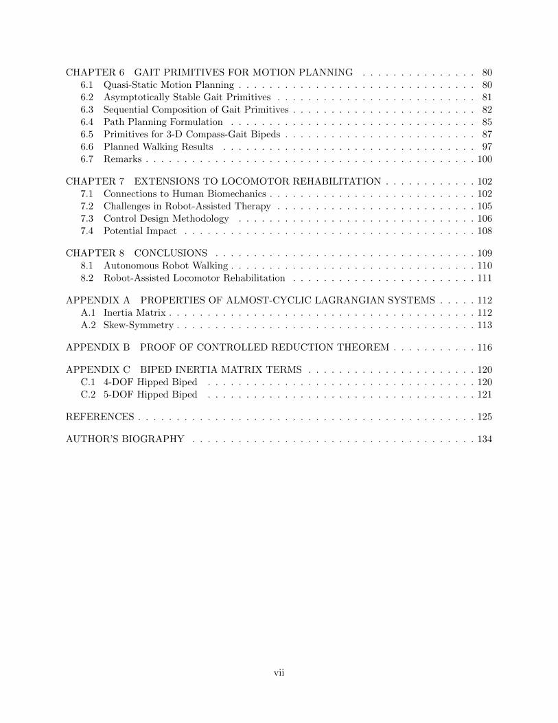
Figure 1.1: The transverse (or axial), frontal (or lateral), and sagittal planes-of-motion of thehuman body [7]. These correspond to the yaw/heading, lean/roll, and pitch degrees-of-freedom,respectively, at the ankle.

D, and control input u is in control space U . An uncontrolled or closed-loop system is represented

as a hybrid system without an explicit control input:

H :

x = f(x) x ∈ D\Gx+ = ∆(x−) x− ∈ G

In the case of an n-degree-of-freedom (DOF) robotic system, the state x = (qT , qT )T ∈ R2n is

composed of the configuration vector q ∈ Rn of joint positions and its tangent vector q ∈ Rn of

joint velocities. We now discuss solution (or integral) curves of hybrid systems in order to define

hybrid limit cycles, our mathematical representation of bipedal walking gaits.

1.1.1 Solutions of hybrid systems

Bipedal walking gaits correspond to periodic solutions of hybrid systems. In particular, bipedal

walking gaits are 2-step periodic (with skew-symmetry between steps) due to bilateral symmetry

seen in the frontal and transverse planes-of-motion in Fig. 1.1.

A solution curve x(t) to a hybrid system H is called a hybrid flow. This is h-periodic if x(t) =

x(t +∑h

i=1 Ti), for all t ≥ 0, where Ti is the fixed time-to-impact between the (i − 1)th and ith

2

discrete events. The image of a periodic hybrid flow in the phase space is an invariant set1 called

the h-periodic hybrid orbit

O =

x ∈ D | x = x(t), t ∈ [0,

h∑i=1

Ti]

. (1.1)

If a periodic hybrid orbit is isolated, rather than one in a continuum of orbital solutions, it is called

a hybrid limit cycle of H .

1.1.2 Orbital stability

We must consider orbital stability of hybrid limit cycles in order to account for perturbations in

bipedal locomotion. An h-periodic hybrid orbit O is said to be (locally) asymptotically stable if all

hybrid flows initiated in a neighborhood of O asymptotically approach the orbit. To be precise, we

define a stronger sense of stability: an h-periodic hybrid orbit O is (locally) exponentially stable if

there exist constants k, α, γ > 0 such that for all hybrid flows x(t) with d(x(t0),O) < γ,

d(x(t),O) ≤ ke−α(t−t0)d(x(t0),O) (1.2)

for all t ≥ t0. The distance function from vector x to set O in Euclidean metric space (R2n, d) is

defined as d(x,O) := infy∈O ||x− y||.The stability of periodic hybrid orbits is determined using the method of Poincare sections [6],

which analyzes the Poincare map P : G→ G associated with hybrid system H . This is a discrete

map defined on the Poincare section, naturally chosen to be guard G, which characterizes the

evolution of a hybrid flow between intersections with G. In particular, the h-composition of this

map sends state xj ∈ G ahead h impact events by the discrete system xj+h = P h(xj). In the

case of an h-periodic hybrid orbit O, we have an h-fixed point x∗ ∈ G ∩ O such that x∗ = P h(x∗).

We then know that periodic hybrid orbit O is locally exponentially stable (LES) if and only if the

associated fixed point x∗ is LES in the discrete-time system defined by Poincare map P .

Although we cannot analytically calculate this nonlinear map to determine its stability about

x∗, we can numerically approximate it through simulation. This allows us to locally analyze orbital

stability as a linear discrete system by the map’s linearization, δP h, where exponential stability

is equivalent to the eigenvalue magnitudes of δP h being strictly within the unit circle. The local

1In the analogous case of continuous-time systems, this would be a compact set defined by a closed trajectory [8].

3

stability region about h-fixed point x∗, known as the basin of attraction, is defined as

BoA(x∗) =x ∈ G s.t. lim

z→∞P hz(x) = x∗

. (1.3)

We defer the numerical details of simulation-based Poincare analysis to [4, 9].

This mathematical representation of walking gaits applies to multiple forms of bipedal loco-

motion. In order to provide context and motivation for studying dynamic locomotion, we first

distinguish this mode of transportation from quasi-static walking.

1.2 Quasi-Static Walking

Many sophisticated humanoid robots, such as HRP-2 [10] and Honda ASIMO [11], have demon-

strated robotic bipedal walking that is not dynamic. Rather, the motion of these robots is con-

strained by “quasi-static” equilibrium conditions related to the zero moment point (ZMP).

A walking mechanism resists gravity by applying force against the ground, resulting in an equal

and opposite reaction force acting at a point called the center of pressure (CoP) inside the support

polygon/footprint, i.e., the convex hull of the ground contact area(s). In order for the biped to

remain statically balanced (i.e., no foot rotation), there must be zero net moment at the CoP:

M +R× F = 0, (1.4)

where the walking mechanism contributes (linear) force vector F and moment vector M at the

ankle, and R is the vector defined from the CoP to the center of the ankle.

The nominal point at which condition (1.4) holds is called the foot rotation indicator (FRI) [12].

This point coincides with the CoP when inside the biped’s support polygon. In this case, the

ZMP is said to exist and the foot remains flat on the ground. When the FRI exits the support

polygon, the ZMP disappears and the biped rotates about a new passive DOF at a point or edge

on the boundary of the support polygon. This falling scenario is always avoided by ZMP trajectory

planners, whereas dynamic gaits are largely composed of such pendular falling states.

Definition 2. A quasi-static walking gait is a hybrid limit cycle in which condition (1.4) always

holds. A dynamic walking gait is a hybrid limit cycle in which condition (1.4) is violated for some

portion of the cycle.

4

However, satisfying ZMP condition (1.4) does not necessarily imply stability of the hybrid limit

cycle associated with a quasi-static gait [6, Section 10.8]. This form of locomotion also requires

large actuators to track constrained reference joint angles/velocities while actively supporting the

body weight with flexed knees during the entirety of each step cycle [13, 14]. This results in

unnatural shuffling motion that is up to an order of magnitude less efficient than dynamic walking

in terms of specific energetic cost of transport (energy consumed per unit weight per unit distance)

[15]. Arguably, ZMP gaits may have a closer resemblance to the inefficient postural attributes of

chimpanzee bipedalism – these hunched gaits similarly have flexed knees that never pass beneath

the hip joint, preventing the pendular falling motion of dynamic walking gaits [16].

However, ZMP control strategies have dominated humanoid applications requiring motion plan-

ning, such as locomotion with obstacle avoidance in three-dimensional (3-D) space [17,18], interac-

tion with complex environments [19,20], and walking and climbing on rough terrain [21,22]. These

practical applications have historically proven more difficult to achieve with dynamic walkers, which

we wish to address in this thesis.

1.3 Dynamic Walking

In principle, dynamic walking embraces ballistic momentum and gravitational potential energy for

speed and energetic efficiency (in fact, gravity provides the only power source in passive walking

down shallow slopes [3]). This has been exploited by active robot control strategies that shape the

potential energy into different forms, such as rotating the gravity vector to enable pseudo-passive

dynamic walking on arbitrary slopes (i.e., uphill “feels like” downhill) [23, 24]. These stable gaits

do not track reference patterns, but naturally appear from the system nonlinearities, including the

potential energy.

1.3.1 Planar bipeds

Early work on dynamic walking began with simple serial-chain models, such as the two-link

“compass-gait” biped of Fig. 1.2, constrained to the sagittal plane-of-motion to roughly approxi-

mate human dynamic motion (Fig. 1.1). In the pioneering work on passive walking [3], McGeer

discovered the existence of stable hybrid limit cycles down shallow slopes between about 3 and

5, the range of slope angles for which the potential energy introduced by gravity after each step is

5

M

m ml

z

y

−θs θns

called passivity based nonlinear control. Relatedresults appear in Ohta et al. [1999]. In Suzuki etal. [2001] gravity compensation control is used inconjunction with trajectory tracking. The passivelimit cycle for a McGeer-like planar biped isused as a reference trajectory and a sliding modecontroller is designed to track this trajectory.

Passive walking in three-dimensions was inves-tigated in Kuo [1999]. Passive limit cycles werefound in the lateral plane as well as the saggitalplane. However, the lateral motion was unstableand had to be compensated by feedback control.Kuo used an elegant control algorithm to ad-just the foot placement at each step to achievestable locomotion in both the lateral and sagit-tal planes. More recently, true three dimensionalpassive walking has been achieved in Collins etal. [2001]. This remarkable biped has both kneesand specially shaped feet to stabilize the lateralmotion, arms that swing coupled to the leg motionto stabilize yaw motion and produces surprisinglyanthropomorphic motion without actuation of anykind.

Motivated in part by the above work showingthat passive walking can be achieved in threedimensions, we extend here our previous resultson passivity based nonlinear control to the generalcase of a three dimensional n-DOF biped. Theresult follows nearly identically to the 2-D case asa consequence of some symmetry properties in theEuler-Lagrange equations describing the biped.Specically, we show that changing the groundslope denes a group action on the congurationmanifold of the system and that both the kineticenergy and impact dynamics are invariant underthis group action. Hence, to achieve invariance ofthe passive limit cycles, one need only compensatethe potential energy as in the planar, 2-D case.

2. BACKGROUND

We consider a general n-degree-of-freedom bipedin 3-dimensions. The act of walking involves botha swing phase and a stance phase for each leg aswell as impacts between the swing leg and ground.We make the standard assumptions, namely,

(i) impacts are perfectly inelastic (no bounce),(ii) transfer of support between swing and stance

legs is instantaneous,(iii) there is no slipping at the stance leg ground

contact.

Under these assumptions it can be shown (Hur-muzlu and Moskowitz [1986]) that each impactresults in an instantaneous jump in velocities,hence a discontinuity in kinetic energy. The posi-tion variables are continuous through the impactand so, if the kinetic energy dissipated during the

Fig. 1. A General 3-D Biped

impact is somehow compensated so that the jointangles and velocities after impact are restored totheir original values at the beginning of the step,then a periodic gait (limit cycle) results. In passivewalking this is achieved by starting the bipedon a constant downhill slope so that that lossof kinetic energy is compensated by the changein potential energy during the step. The loss ofkinetic energy can also be compensated by activecontrol of actuators at the joints so that walkingcan be achieved on level ground and/or uphill.

2.1 Group Actions and Invariance

Group Actions

We now give some background from dierentialgeometry and dynamical systems theory (see Mars-den and Ratiu [1999], Olver [1993]).

Denition 2.1. Let Q be a dierentiable manifoldand G be a Lie group. Then G is said to act onQ if there is a mapping : G Q ! Q taking apair (g; q) to (g; q) = g(q) and satisfying for allq 2 Q

(i) e(q) = q, where e is the identity element ofG, and

(ii) g1(g2(q)) = g1g2(q).

A group action on Q induces corresponding mapson scalar functions over Q (e.g., the system'skinetic and potential energy), tangent vectorsand vector elds (e.g., the system's instantaneousvelocity), and one forms (e.g., the external forcesapplied to the system). For example, if h : Q! <is a scalar function on Q, then the group actioninduces a map via composition,

(h Æ)(q) := h((q))

We say that the scalar function h(q) is invariant(under the group action) if, for all g 2 G

Figure 1.2: The two-link “compass-gait” biped constrained to the sagittal plane-of-motion (left)and a general 3-D biped (right).

matched by the energy dissipated at foot impact with ground. Gravity-powered passive walking was

further studied in [4], showing period-doubling (flip) bifurcations in the gait as model parameters

such as slope angle are varied beyond some stability region.

Underactuated planar walking on flat ground was achieved with the method of hybrid zero

dynamics [5,6,25], using output linearization to zero hybrid-invariant output functions (i.e., virtual

constraints) describing some desired gait. This theory was applied to the compass-gait biped with

rigid legs as well as compliant legs to incorporate a nontrivial double-support phase [6,26]. In fact,

hybrid zero dynamics was successfully implemented on the planar RABBIT bipedal robot at the

Laboratoire Automatique de Grenoble in France [27] and more recently on the planar MABEL

biped at the University of Michigan [28].

Terrain uncertainty was confronted in [29] by discretizing the state space and dynamics of the

planar compass-gait biped, so as to analyze the stochastic “metastability” of the resulting controlled

Markov chain. However, the mesh state space expands exponentially with the robot’s dimension-

ality, bringing into question this method’s practicality for high-DOF bipeds in three dimensions.

1.3.2 Three-dimensional walking

Although these various concepts have been successful with regard to planar dynamic walkers, there

has been scattered success in extending these ideas to 3-D space, where robot dynamics become

quite complex with highly-coupled DOFs in three planes-of-motion (Fig. 1.1). Passive dynamic

6

walking was extended to a spatially 3-D biped (modeling pitch and lean without yaw) in [30],

requiring direct control over the leg splay angle and an assumption that the continuous dynamics

are invariant under this actuation. The carefully tuned walking mechanism of [31] demonstrated

3-D passive walking down a particular fixed slope from a specific initial configuration, but its gait

was incredibly sensitive to perturbations and thus prone to falls.

Stochastic reinforcement learning was used to separately compute control policies for the frontal-

and sagittal-plane modes of a simple 3-D biped in [32]. Spatial 3-D walking was similarly achieved

in [33] with a decoupling assumption between the planes-of-motion to separately define virtual

constraints for hybrid zero dynamics. However, we argue that these planes-of-motion are strongly

coupled, especially in the case of significant swaying and steering motions, requiring a more so-

phisticated method of decomposing a biped’s dynamics. This philosophy was embraced in [34,35],

where hybrid zero dynamics was rigorously extended to 3-D bipeds by employing optimization

instead of manual inspection to define the complicated virtual constraints.

The aforementioned energy-shaping methods of [23,24,36], known as controlled symmetries and

passivity-based control, exploit the geometric structure inherent in robot dynamics of arbitrary

dimensionality. Specifically, the first method maps passive limit cycles down shallow slopes to

pseudo-passive limit cycles on arbitrary slopes (with trajectory time-scaling in [37–39]). Passivity-

based energy tracking then expands the small basin of attraction associated with passive limit cycles

to enable stable walking on uneven terrain. However, these tools necessarily require the existence

of stable passive limit cycles, which is usually not the case for complex 3-D bipedal walkers (e.g.,

right side of Fig. 1.2). This has limited the primary application of these energy-shaping approaches

to sagittal-plane walkers such as the compass-gait biped. We wish to extend these satisfying results

to general 3-D walkers.

1.3.3 Motion planning

Some of the biggest challenges in dynamic locomotion concern stable motion planning in complex

or uncertain environments. A rigorous framework for controlling the planned flight trajectories

of planar dynamics runners was developed in [40]. Step-level planning over irregular terrain was

applied to planar dynamic walkers in [41, 42]. However, these methods have not yet scaled to

high-DOF models in 3-D space.

Hybrid zero dynamics has proven successful in constructing LES walking gaits capable of steering

7

Sagittal-plane (2D) walking gait Three-dimensional walking gait

=⇒

Figure 1.3: Controlled geometric reduction: building a 3-D walking gait (right) from asagittal-plane walking gait (left).

to nearby headings in 3-D space [35]. In particular, LES implies local input-to-state stability

(LISS): sufficiently small changes in heading result in small changes in state between impact events.

Unfortunately, it is difficult to find the bounds for this form of stability over arbitrary curved paths

(i.e., what range of initial states will recover from some bounded sequence of steering angles).

In fact, we are unaware of any path planning results for directional dynamic walking in 3-D space,

aside from the work [43] to be revisited in this thesis. The lack of related work is likely due to

challenges in creating dynamic gaits for fully 3-D bipedal robots, where additional yaw dynamics

must be controlled to variable headings with some sense of stability.

1.4 Contributions of the Thesis

Despite the minute class of 3-D bipeds that can stably exploit passive dynamics, symmetry- and

passivity-based methods remain appealing due to the natural and efficient dynamic gaits they pro-

duce for planar robots. The existence problem of passive limit cycles for 3-D bipeds was addressed

with a controlled form of symmetry-based geometric reduction in [44–46]. In particular, energy-

shaping control was used to decouple a spatially 3-D biped’s sagittal plane-of-motion, which is well

studied with known limit cycles, and from this build pseudo-passive walking gaits for the full-order

system. We generalize these reduction-based control results throughout this thesis to consider fully

3-D bipeds and curved walking paths as in Fig. 1.3.

8

1.4.1 Reduction-based control

We present the energy-based method of controlled geometric reduction, which is fundamentally

related to the geometric properties of symmetry and passivity. Given a mechanical system char-

acterized by its Lagrangian function L = K − V or Hamiltonian function H = K + V (for kinetic

energy K and potential energy V), we consider symmetries in the form of cyclic variables q1, which

do not explicitly appear in the Lagrangian or Hamiltonian functions:

∂L∂q1

= 0 ⇐⇒ ∂H∂q1

= 0. (1.5)

Passive feedback in an energy-shaping control law establishes a functional momentum conserva-

tion law that optimally controls cyclic variables to set-points or limit cycles. This nonholonomic

constraint (an invariant) defines a lower-dimensional zero dynamics corresponding to the original

robot with the first DOF fixed.

We show that a stabilizing controlled reduction can be designed based on a passivity-based

feedback transformation of L into a special form of controlled Lagrangian with broken symmetry:

Lλ(q, q) = Kλ(q, q) +Qλ(q)q − Vλ(q), (1.6)

depending on some desirable function λ of the cyclic variables. This almost-cyclic Lagrangian

system in closed loop corresponds to an equivalent Hamiltonian system with upper-triangular form,

showing that full-order stability is provided in a manner analogous to backstepping (specifically,

forwarding control) [8,47]. By choosing the biped’s sagittal plane as the desired zero dynamics, we

can exploit the minimum phase property provided by the existence of passive limit cycles.

We then generalize this theory for recursive decoupling of subsystems as in [48, 49], allowing

application to completely 3-D bipeds with both yaw and lean modes (respectively in the frontal

and transverse planes of Fig. 1.1). This method exploits symmetries inherent in serial kinematic

chains, but human morphology involves a significantly more complex branching tree structure (i.e.,

a branched chain). Therefore, multistage controlled reduction is extended to the class of open

kinematic chains [50], such as robots with torsos and articulated arms (e.g., right side of Fig. 1.2).

This simplifies the search for full-order hybrid limit cycles and significantly expands the class of

3-D bipeds that can achieve pseudo-passive dynamic walking.

9

1.4.2 Path planning

We will use reduction-based control to construct straight-ahead walking gaits corresponding to LES

hybrid limit cycles [48, 49], which can be steered toward arbitrary headings as illustrated in Fig.

1.3. These results will be extended to show that constant-curvature steering between steps induces

LES hybrid limit cycles (modulo yaw) corresponding to circular turning [50,51]:

x∗tu(s) + (s 02n−1)T = P htu(s)

(x∗tu(s)

), (1.7)

where s is the constant steering angle resulting in h-fixed point x∗tu(s) for an n-DOF robot walker.

However, walking paths can entail an arbitrary sequence of turning motions that may accumulate

perturbations and lead to instability.

In order to build bipedal robots that can quickly and efficiently navigate through real-world

environments, the stability of dynamic walking must be considered when planning walking paths

with significant steering. This is no trivial task, as turning motion inherently deviates from known

hybrid limit cycles associated with straight-ahead walking [51]. Unlike ZMP methods, the robot

state cannot be checked against closed-form balance conditions like (1.4). The hybrid nonlinear

dynamics of a dynamic walker make it difficult to analytically assure stability2 – the fate of a

walking trajectory from given initial conditions is usually computed in simulation [4, 9].

Therefore, we present a hierarchical control and planning framework for 3-D dynamic locomo-

tion. Given a low-level controller that produces a set of asymptotically stable gait primitives, a

dynamic walker can be controlled as a discrete-time switched system that sequentially composes

gait primitives from step to step [43]. Each gait primitive is a pair G = (P hcl, x∗), where x∗ is an

asymptotically stable h-fixed-point (modulo yaw) of the closed-loop Poincare map Pcl for some

walking strategy. Motivated by the controller composition method of Lyapunov funneling [52], we

derive rules by which a planned walking path that is a sequence of these primitives (e.g., Fig. 1.4)

may be stably followed by the robot.

The continuously parameterized set of primitives Ps = Gst,Gtu(s),Gtu(−s) is associated with

a nominal set of constant-curvature arcs on the walking surface, growing a discrete tree with

branching factor three. Hence, dynamically stable path planning reduces to a discrete tree search

that explores the action space of primitive arcs. This result enables motion planning for fast and

efficient dynamic walkers in a similar manner to what is already possible for quasi-static walkers.

2This challenge is not limited to dynamic walking – ZMP condition (1.4) does not necessarily imply stability [6].

10

Gtu(s)

Gtu(−s)

Gtu(0)

V (x0)

V (x∗tu(-s))

V (x∗tu(0))

V (x∗tu(s))

Figure 1.4: Sequential composition of Lyapunov funnels, each being the graph of a Lyapunovfunction over its state space (illustrated as circular neighborhoods in a planar global space). Thefunneled state trajectory (dotted green) corresponds to the trajectory of the funneled Lyapunovfunctions (solid blue). Original figure from [52] reproduced with permission of the publisher.

1.5 Organization of the Thesis

We begin the thesis with a background review of the geometric notions of passivity, symmetry,

and reduction in Chapter 2. This leads to our Lagrangian and Hamiltonian formulations of con-

trolled geometric reduction in Chapter 3, by which we establish unifying connections to passivity

and symmetry. We present the multistage application of controlled reduction to mechanical sys-

tems in Chapter 4, identifying symmetries to control the large class of open kinematic chains as

lower-dimensional subsystems. We then introduce the primary application of the thesis in Chap-

ter 5: the 4-DOF and 5-DOF bipedal walkers, their general control law, and simulation results

of straight-ahead walking and turning in 3-D space. This motivates the sequential composition

theory of asymptotically stable gait primitives in Chapter 6, including planned walking results for

the hipless 4-DOF and 5-DOF compass-gait bipeds. We compare these results to human biome-

chanics and propose extensions of the energy-shaping control paradigm to robot-assisted locomotor

rehabilitation in Chapter 7. We conclude in Chapter 8 with remarks on the significance of this

material and the future work it motivates.

11

CHAPTER 2

PASSIVITY AND SYMMETRY IN MECHANICAL SYSTEMS

Although mechanical systems often have complex nonlinear dynamics, they are rich with geometric

structure that can be exploited for control and analysis independent of specific dynamic models.

For example, the notion of passivity allows an energetic interpretation of system dynamics using

common Lyapunov and L2-gain methods [8, 53–55]. In other words, a complex nonlinear system

can be studied much like an RLC circuit or spring-damper system. Nonlinear passivity-based

control methods provide stability with larger basins of attraction and better robustness to model

uncertainty [56–59] than that possible with linear methods. This has enabled oscillatory pattern

generation for locomotion [36, 37] and synchronization [60]. It has also been shown that optimal

feedback control is directly related to passive outputs [61], demonstrating the importance of this

structural property for both linear and nonlinear systems.

Geometric reduction is another classical tool, used to analytically decompose the calculation

of integral curves of a physical system with symmetries. These systems are characterized by La-

grangian or Hamiltonian functions that are invariant under the action of a symmetry group on the

configuration space [62–64]. For example, in the case of Routhian reduction, a Lagrangian function

has no dependence on so-called cyclic variables, so the system is invariant under the action of

rotating these variables. By dividing out the coordinates corresponding to such symmetry groups,

integral curves can be solved in a lower-dimensional space that uniquely characterize the full-order

solution. Complex symmetry groups can also be decomposed into subgroups for dynamical reduc-

tion by stages as discussed in [63,64].

A topological perspective was used in [65] to show a lower bound on dynamic model reduction of

serial kinematic chains based on kinematic models, by which reduced adaptive control algorithms

are designed. A similar concept not directly related to symmetry is differential flatness, describ-

ing nonlinear (control) systems whose integral curves are in smooth one-to-one correspondence

with arbitrary curves of a lower-dimensional space [66]. The full-order space is mapped to the

12

lower-dimensional space by so-called flat outputs, which are functions of the system state and their

derivatives. From these outputs and their derivatives, the full-order state can be solved without

integration. Although this property is not necessarily based on symmetries, [67] shows its appli-

cation to a special class of mechanical systems with symmetry and one degree of underactuation

(e.g., underwater vehicles). This method is helpful for simplified trajectory planning [68], but in

general, differential flatness is difficult to determine and characterize with appropriate outputs.

The properties of symmetry and passivity are easy to identify and provide model-independent

structure, motivating analysis and control methods like controlled geometric reduction. Therefore,

this chapter offers a background discussion to define these geometric properties. We begin with

two important formulations of the dynamics of mechanical systems: Lagrangian and Hamiltonian

mechanics. The resulting dynamics are equivalent, but each method offers a different perspective

that will prove useful for exploiting passivity and symmetry.

2.1 Lagrangian Mechanics

An n-DOF mechanical system with configuration space Q is described by elements (q, q) of tangent

bundle1 TQ and Lagrangian function L : TQ → R, given in coordinates by

L(q, q) = K(q, q)− V(q) (2.1)

=1

2qTM(q)q − V(q),

where K(q, q) is the kinetic energy, V(q) is the potential energy, and n × n symmetric, positive-

definite M(q) is the generalized mass/inertia matrix. By the least action principle [62], system

integral curves necessarily satisfy the Euler-Lagrange (E-L) equations

E L q L :=d

dt∇qL −∇qL = τ, (2.2)

where n-dimensional vector τ contains the external joint torques. This second-order system of

ordinary differential equations (ODEs) directly gives the dynamics for the actuated mechanism in

phase space TQ. These equations have the special structure

M(q)q + C(q, q)q +N(q) = Bu, (2.3)

1The space of configurations and their tangential velocities.

13

where n×n-matrix C(q, q) contains the Coriolis/centrifugal terms, vector N(q) = ∇qV(q) contains

the potential torques, and n×m-matrix B (full row rank) maps actuator input vector u ∈ Rm to

joint torques τ = Bu ∈ Rn for m ≤ n. We initially consider the case of full actuation (m = n

implying that B is invertible), so we take B to be identity without loss of generality.

These dynamics yield control system (f, g) on TQ:

q

q

= f(q, q) + g(q)u, (2.4)

with vector field f and matrix g of control vector fields:

f(q, q) =

q

M(q)−1 (−C(q, q)q −N(q))

g(q) =

0n×n

M(q)−1

.

Defining state x = (qT , qT )T ∈ TQ, this takes the form of a first-order differential control system.

For the analytical results in Chapters 2-4, we make the standard assumption of local Lipschitz

continuity. We later present numerical results for hybrid systems with Lipschitz continuous phases

in Chapters 5 and 6 – analytical results are possible in this context with a special case of controlled

reduction as seen in [45].

2.2 Hamiltonian Mechanics

The Hamiltonian formulation begins with the Hamiltonian function, representing the system’s

mechanical energy:

H = K + V = L+ 2V.

This quantity is more useful when expressed in terms of the system’s generalized momentum,

defined as

p = J (q, q) := ∇qL(q, q), (2.5)

= M(q)q

14

where momentum map J expresses p in terms of Lagrangian coordinates (q, q). The phase space

of the system can then be expressed in canonical coordinates (q, p) of the cotangent bundle2 T ∗Q.

In these coordinates, Hamiltonian H : T ∗Q → R is obtained from a Lagrangian L by a Legendre

transformation:

H(q, p) =[pT q − L(q, q)

]∣∣p=J (q,q)

=1

2pTM−1(q)p+ V(q). (2.6)

Note that the sign of the Hamiltonian function (and thus the Legendre transformation) is merely

a convention, and in some cases it is convenient to use the opposite sign.

The controlled dynamics are given by Hamilton’s equations, two coupled first-order ODEs:

q

p

=

0n×n In×n

−In×n 0n×n

∇qH∇pH

+

0n×1

u

(2.7)

where control u enters into the derivative of the generalized momentum, known as the Newtonian

forces (or torques). Note that direct calculation gives ∇pH = M−1(q)p, and the right-hand side of

(2.7) defines the covector field on Q.

2.3 Passivity

Given either mechanics formulation, we can define a first-order control system with an output:

x = f(x) + g(x)u (2.8)

y = h(x),

where x ∈ R2n and u, y ∈ Rn. In this context, the notion of passivity offers an energetic perspective

based on common Lyapunov methods [36].

Definition 3. Control system (2.8) is (input/output) passive if there exists a differentiable non-

negative scalar function S : R2n → R, called the storage function, such that S ≤ yTu.

Lemma 1. Suppose (2.8) is passive with storage function S. Given output feedback control

u = γ(y), where γ is any continuous function satisfying yTγ(y) ≤ 0, the origin is stable in the sense

2The space of configurations and their conjugate momenta.

15

of Lyapunov, i.e., for every ε > 0 there exists a γ > 0 such that if ||x(0)|| < γ then ||x(t)|| < ε for

all t > 0. Moreover, the zero level-set x|γ(h(x)) = 0 is asymptotically attractive.

This classical result is proven in [8,54]. It is important to note that this offers no further stability

guarantees on the attractive zero level-set, and these so-called zero dynamics are a common topic

of study, e.g., [5, 6, 36,45].

Passivity also has interesting connections with optimal control discussed in [61]. Given perfor-

mance index

J(x0) =1

2

∫ ∞0

(l(x)T l(x) + uTu)dτ, (2.9)

if a differentiable optimal function V (x) = minu(·) J(x) exists, then the optimal feedback control

has the form [54]

u = −LgV (x) := −∇xV g(x), (2.10)

where LgV is the Lie derivative of function V with respect to vector field g. It is shown in [61]

that the optimal system has a passivity property with respect to output y = h(x) = LgV (x).

Conversely, given a feedback control law u∗ = −k(x), a pair V (·), l(·) for which (2.9) is minimized

by u∗ is known as the solution to the inverse optimal control problem. This is similarly related to

passivity [61]:

Theorem 1. A necessary/sufficient condition for the existence of a solution to the inverse optimal

control problem of system (2.8) with u∗ = −k(x) subject to (2.9) is that the following system is

passive with respect to input v:

x = f(x)− g(x)k(x) + g(x)v (2.11)

y = k(x).

Given state x = (qT , qT )T ∈ TQ, a structural property of robots shows input/output passivity for

y = q, since the Hamiltonian H (i.e., total energy) acts as a storage function: H = qTu for vector u

of input torques [55]. For any nonpositive passive feedback law γ(q) ≤ 0, we have H = qTγ(q) ≤ 0

providing Lyapunov stability by Lemma 1. If this law is negative-definite, then this further shows

asymptotic dissipation of joint velocities: q → 0. In fact, we find that linear γ is optimal by

16

Theorem 1:

Proposition 1. Linear output feedback u = −q is the optimally stabilizing control (in the sense

of Lyapunov) of a robot with respect to (2.9) for l(x) = q.

Proof. Hamiltonian H is our value function. Using the robot passivity property, [61, Theorem 1]

tells us that k(x) = LgH = q and lT (x)l(x) = −LfH + LgkH = qT q since LfH = 0 (conservation

of energy). Based on candidate optimal feedback law k(x) = q, we can define v = u+ q for system

(2.11):

x = f(x)− g(x)k(x) + g(x)v

= f(x) + g(x)u.

This is the original robot system with input u and output y = q, so H = qT u = qT v− qT q, implying

H ≤ qT v and satisfying passivity for (2.11). Hence, u∗ = −k(x) is stabilizing by Lemma 1 and

optimal by Theorem 1.

Note that this passive feedback can be implemented mechanically with a rotary (or linear)

damper. We now discuss the notion of symmetry in order to connect these properties to symmetry-

breaking control.

2.4 Symmetry

We introduce the notion of symmetry with some basic concepts from differential geometry (cf.

[62, 69–71]), starting with formalisms from group theory.

Definition 4. A set G together with a binary operation defined on elements of G is called a

group if it satisfies the following four axioms:

1. Closure: If g1, g2 ∈ G, then g1 g2 ∈ G.

2. Identity: There exists an identity element, e ∈ G, such that e g = g for every g ∈ G.

3. Inverse: For each g ∈ G, there exists a unique inverse, g−1 ∈ G, such that gg−1 = g−1g = e.

4. Associativity: If g1, g2, g3 ∈ G, then (g1 g2) g3 = g1 (g2 g3).

17

Groups define actions on sets (which may also be groups), such as rotations in a configuration

space. Since we are interested in differential systems, we also show how these group actions induce

maps on tangent spaces [24].

Definition 5. A group G is said to act on another set Q (through a group action) if each element

g ∈ G defines a bijective mapping Φ : G × Q → Q taking a pair (g, q) to Φ(g, q) = Φg(q) and

satisfying for all q ∈ Q:

1. Φe(q) = q, where e is the identity element of G.

2. Φg1(Φg2(q)) = Φg1g2(q).

Definition 6. Let TqQ be the linear space of tangent vectors at q, and let TQ =⋃q TqQ be the

tangent bundle of Q. Letting g ∈ G, we then denote TqΦg as the tangent function to Φg mapping

TqQ onto TΦg(q)Q. This defines the lifted action TΦ : G× TQ → TQ.

In the context of differential calculus, we consider continuous Lie groups, which are smooth

manifolds (cf. [62, 69]). Common examples are SO(n), the group of orthogonal orientations (or

rotations) in n dimensions with matrix multiplication as the group operation; S1, the group of

rotations about the unit circle with scalar addition; and Rk, the group of Euclidian translations

with vector addition. Such a group G is called a symmetry group if a function is invariant under

its action:

Definition 7. Let F : M → N be a smooth mapping between manifolds M and N and let

Φ : G ×M → M be an action of the Lie group G on M . Then, we say that F is invariant under

the group action if F Φ = F , i.e., if for all g ∈ G and m ∈M , (F Φg)(m) = F (m).

For a smooth vector field3 X mapping Q to TQ, this definition of invariance corresponds to

X(Φg(q)) = TqΦg(X(q)) = X(q),

for all g ∈ G, q ∈ Q. I.e., lifted action TqΦg is the identity map. In the Hamiltonian framework,

this is similarly the case for a covector field Y on Q, where T ∗q Φg = I. This definition can be

relaxed to the case of equivariance where TqΦg is not always identity. However, this thesis will

3Given a configuration space Q, Lagrangian mechanics define TQ as the state space, so vector fields map TQ toa 2nd-order tangent space. The definitions of invariance in this section apply to Lagrangian mechanics if we relabelthis state space to be set Q.

18

only consider group actions Φ that are commutative on Q, implying that the lifted action is indeed

identity. An important implication of invariance is the following:

Lemma 2. Let vector field X be Φ-invariant, and let γ : [0, T ] → Q be an integral curve of X.

Then, for all g ∈ G, Φg γ is also an integral curve of X.

Uniqueness of solutions to X tells us that, if γ has initial condition γ(0), then Φgγ is the integral

curve from initial condition Φg(γ(0)). Hence, X has no isolated stable solutions in full-order space.

Rather, we may find infinitely many fixed-points or periodic orbits. We will revisit this implication

shortly.

2.5 Geometric Reduction

Geometric reduction requires the existence of symmetry in a mechanical system’s dynamics, which

induces an invariant submanifold4 in phase space TQ. Symmetries are often found in the form

of conservation laws, where a physical quantity of the system is conserved by the dynamics [70].

Therefore, these conservation laws can be expressed as nonholonomic constraints of the first-order

form Jc(q)q = b(q) or second-order form Jc(q)q = b(q, q). If constraint Jacobian Jc has row rank k

in the former case, then the system dynamics restricted to the invariant surface

Z = (q, q)|Jc(q)q = b(q) (2.12)

give a reduced-order system of dimension n − k. The constraints then uniquely describe the “di-

vided” coordinates, qc ∈ Rk, based on the reduced coordinates, qr ∈ Rn−k, where q = (qTc , qTr )T .

In classical Routhian reduction [62], a Lagrangian L has configuration space Q = G×S (say, an

n-torus), where G = Tk = S1× . . .×S1 is the configuration symmetry group and S ∼= Q\G = Tn−k

is the shape space. Symmetries of L are characterized by cyclic variables qc ∈ G, such that

∇qcL = 0. (2.13)

The symmetry group G acts on Q by rotating the cyclic coordinates, i.e.,

Φg(q) = (q1 + g1, . . . , qk + gk; qk+1, . . . , qn)T (2.14)

4A submanifold of manifold TQ is a subset which itself has the structure of a manifold. Any system trajectoryinitialized in an invariant submanifold will remain in the submanifold for all time.

19

for g ∈ G and q ∈ Q. The lifted action induced on TQ is the identity map TqΦg(q) = q. Then, the

Lagrangian is invariant under this rotating action:

(L Φg)(q, q) = L(Φg(q), TqΦg(q))

= L(Φg(q), q)

= L(q, q) (2.15)

for all g ∈ G and (q, q) ∈ TQ. The second equality follows from identity of the lifted action.

Recalling that Lagrangian L has no dependence on qc by (2.13), the last equality follows from the

group action (2.14) rotating only these cyclic variables. A similar statement can be made about

invariance of the corresponding vector field.

If the Lagrangian has cyclic variables that are free from external forces (e.g., no actuation), we can

decompose the dynamics with Routhian reduction. Equation (2.13) implies that momentum vector

pc conjugate to the cyclic coordinates is equal to some constant vector µ. The dynamics then evolve

on invariant level-set Z of these conserved momentum quantities, where Jc = [Ik×k 0k×n−k]M

and b(q) = µ in (2.12). Based on these constraints, we can directly relate full-order integral curves

on phase space TQ to reduced-order integral curves on phase space TS, and vice versa. In other

words, we divide out group G by projecting TQ onto reduced space TS. However, stability in TQmodulo G allows arbitrary drift along orbits of G by Lemma 2, and these divided coordinates often

correspond to unstable modes.

Control can break the symmetry of group G and stabilize orbits of TG, as applied to wave

equations in [72]. The energy of underwater vehicles is shaped with symmetry-breaking potentials

to obtain stability in [73]. Similarly, controlled reduction shapes system energy to stabilize bipedal

walking gaits in three-dimensional space [44–46, 48–51]. We revisit controlled reduction by first

developing a passive-feedback control law to generate new invariants that control cyclic coordinates

to set-points or periodic orbits. We then show that this corresponds to a form of symmetry-breaking

that preserves the projection map for dividing out group G of “almost-cyclic” variables.

20

CHAPTER 3

CONTROLLED GEOMETRIC REDUCTION

Geometric control methods exploiting passivity, symmetry, and system energetics have been widely

studied in the literature. In many cases, symmetry groups correspond to the coordinates of un-

stable and/or unactuated modes (e.g., rotation at the contact between a biped’s toe and ground).

Symmetry-based reduction was elegantly applied to geometric motion planning of underactuated

mechanical systems in [74, 75], using the reduced system to produce motion along unactuated

coordinates corresponding to the symmetry group (but without considering stability). From the

dynamics perspective, a class of planar systems with unactuated cyclic variables were shown to

have relative degree three, allowing asymptotic stabilization and tracking of these variables [40].

In the energetic approach of [58, 59], interconnection and damping assignment (IDA) passivity-

based control shapes an underactuated system’s Hamiltonian function and injects damping via

passive feedback to achieve asymptotic stability. Closely related work [76] uses energy-shaping

control to obtain controlled Lagrangian systems to guarantee stability modulo the symmetry group

(i.e., in a reduced phase space). Reduction theory for controlled Lagrangian or Hamiltonian systems

with symmetry was developed in [77], and potential shaping was used in [73,78] to break symmetry

in order to stabilize the divided coordinates in addition to the reduced phase space.

We are interested in the controlled form of geometric reduction, termed functional Routhian

reduction, which was developed in [44–46, 48–51] to build stable limit cycles for bipedal walking

robots based on stable limit cycles in the sagittal plane-of-motion. This chapter revisits con-

trolled reduction to establish connections to passivity, inverse optimality, and symmetry discussed

in the previous chapter.We first offer a Hamilton-Lagrange perspective to show that passive feed-

back establishes a functional momentum conservation law that optimally controls cyclic variables.

Based on this conservation law, we define the controlled reduction from a full-order system to

its reduced-order subsystem. This allows the desired properties of a controlled reduction to be

specifically designed and achieved through a passivity-based feedback transformation of the system

21

Lagrangian into a controlled Lagrangian with broken symmetry, known as an almost-cyclic La-

grangian. This uniquely corresponds to an almost-cyclic Hamiltonian, by which we establish a new

passivity property and connections to IDA passivity-based control [58, 59]. A change of canonical

coordinates results in upper-triangular form in this closed-loop Hamiltonian system, showing that

full-order stability is provided in a manner analogous to forwarding control [8, 47].

3.1 Control of Cyclic Variables

In this section, we use mechanically-realizable passive feedback to control a scalar cyclic variable

in systems with symmetry (the vectorized case follows analogously and the recursively cyclic case

is considered in [79]). To begin, we define an n-DOF robot’s configuration space Q = Tn with

configuration vector q = (q1, qT2 )T , where scalar q1 is the first coordinate and vector q2 ∈ Tn−1 con-

tains the remaining n−1 coordinates. Assuming that q1 is a cyclic coordinate, we have Lagrangian

invariance under the group action of S1 for rotating the cyclic variable: L(q, q) = L(Φg(q), TqΦg(q))

for all g ∈ S1, (q, q) ∈ TQ, where Φg(q) = (q1 + g, qT2 )T and TqΦg = I.

This further implies that the inertia matrix is cyclic and can be expressed as

M(q2) =

m1(q2) M12(q2)

MT12(q2) M2(q2)

. (3.1)

Here, m1(·) is the scalar self-induced inertia term of coordinate q1, and M12(·) ∈ Rn−1 is the

row vector of inertial cross-coupling terms between q1 and coordinates q2. Moreover, M2(·) ∈R(n−1)×(n−1) is the symmetric positive-definite inertia submatrix of coordinates q2. From the

properties of inertia matrices [55], we know that inertia term m1 is bounded above and below:

m1 < m1(·) < m1, (3.2)

implying that

1

m1<

1

m1(·) <1

m1

, (3.3)

for some constants such that 0 < m1 < m1 <∞.

Based on the definition (2.5), the first pair of canonical coordinates, (q1, p1), is related to the

22

Lagrangian coordinates by the momentum map:

p1 = J1(q, q) := ( 1 0n−1 )M(q2)q

= m1(q2)q1 +M12(q2)q2. (3.4)

Rearranging terms, this is equivalent to the first-order expression

q1 =1

m1(q2)(p1 −M12(q2)q2). (3.5)

The right-hand side of (3.5) is invariant under rotations of q1. Moreover, (2.2) and (2.13) show

that the rate of change in momentum p1 is equal to the first control torque:

d

dt

∂L∂q1

=d

dtp1 = u1.

From the Hamiltonian perspective, ∂H/∂q1 = 0 in (2.7) implies p1 = u1. When control u1 = 0, this

establishes a momentum conservation law (p1 is constant). Therefore, q1 naturally evolves by (3.5)

in one of infinitely many invariant sets (q, q)|J1(q, q) = µ, depending on momentum constant µ.

Many systems have unactuated cyclic variables and actuated shape variables, such as the Acrobot

[80, 81] constrained to the transverse plane (orthogonal to gravity) and bipedal runners in flight

phase [40]. These underactuated systems similarly conserve an angular momentum quantity. This

was exploited in [40] to construct a reduced system and derive conditions for the existence of a

set of outputs yielding an empty zero dynamics. The authors further showed that a dynamic

extension renders these underactuated systems feedback linearizable to provide controllability of

the reduced system. A rotary spring attached between the fixed base and first link then breaks the

momentum conservation law to stabilize the full-order system about an equilibrium. In the next

section, we consider a slightly different approach, using passive damping in input u1 to control the

cyclic coordinate by replacing the existing conservation law with a new functional momentum law.

23

3.1.1 Passive-feedback control

Starting with some scalar linear function of the cyclic variable, λ(q1) = −c(q1 − q1) with q1 and

c > 0 constant, consider the passive-feedback control

u1 =d

dtλ(q1) = −cq1, (3.6)

where ∂λ∂q1

= −c, implying that

p1 = −cq1. (3.7)

Recall that (3.6) is the first term of feedback law γ(q) = −cq, which is associated with a scaled

inverse-optimal solution. This non-zero u1 violates conservation of angular momentum p1.

At first glance, we see that this implies instantaneous mechanical power

H = qT ( −cq1 0n−1 ) = −c(q1)2 ≤ 0, (3.8)

so the system is trivially stable in the sense of Lyapunov and q1 converges to zero by Lemma 1.

Further analysis shows that the generalized momentum now evolves according to

p1(t) = p1(t0) +

∫ t

t0

∂λ

∂q1q1(τ)dτ

= p1(t0) +∂λ

∂q1(q1(t)− q1(t0))

by the fundamental theorem of calculus. Given initial boundary condition

p1(t0) = λ(q1(t0)), (3.9)

it follows that

p1(t) = λ(q1(t)) (3.10)

for all t ≥ t0.

24

Hence, passive control (3.6) produces the functional conservation law

J1(q, q) = −c(q1 − q1) (3.11)

in phase space TQ for some choice of q1 satisfying the initial boundary condition (3.9). Every

initial condition has an associated conservation law, so we have generated infinitely many invariant

submanifolds parameterized by q1:

Zq1 = (q, q)|J1(q, q) + c(q1 − q1) = 0 . (3.12)

This is known as a foliation of the manifold TQ [82]. Given initial conditions in some Zq1 , (3.4)-(3.5)

show that trajectories satisfy the constraint equation

q1 =−c

m1(q2)(q1 − q1)− 1

m1(q2)M12(q2)q2, (3.13)

depending on almost-cyclic variable q1. This constraint is not invariant under the rotating action

of the cyclic coordinate group – the new conservation law does not possess the symmetry. This

will be related to the typical notion of breaking Lagrangian invariance in Section 3.2.

Integral curves (q1(t), q1(t)) and (q2(t), q2(t)) typically must be solved simultaneously in sys-

tem (2.3), so constraint equation (3.13) is nonholonomic (non-integrable). However, given some

assumptions on reduced coordinate pair (q2, q2), e.g., properties provided by reduction, we can

show several stability results for the first DOF based on negative-gain linearity in constraint

equation (3.13). It will be convenient to express these results in terms of the first canonical

pair (q1, p1) in the phase space T ∗Q projected onto T ∗S1, where we can define invariant surface

Dq1 = (q1, p1) | p1 + c(q1 − q1) = 0 from (3.11). Since Dq1 defines a bijective mapping between

canonical coordinates q1 and p1, (3.13) is equivalent to constraint equation

p1 =−c

m1(q2)p1 +

c

m1(q2)M12(q2)q2. (3.14)

3.1.2 Special case without inertial cross-coupling

When M12(·) ≡ 0, some immediate properties of these subsystems follow:

Lemma 3. Given M12(·) ≡ 0, q1 = q1 is the unique equilibrium point of (3.13). Equivalently,

25

p1 = 0 is the unique equilibrium point of (3.14). Moreover, (q1, 0) ∈ Dq1 .

Proof. The LTV gains of (3.13)-(3.14) are strictly bounded away from zero by (3.3), so it is clear

that q1 = q1, p1 = 0 are the unique equilibrium points for their respective systems. The equivalence

implication is provided by the bijective mapping of p1 = λ(q1) = −c(q1 − q1). Finally, λ(q1) = 0

shows the last claim.

Standard results for LTV systems (cf. [8]) show that subsystems (3.13)-(3.14) are stable about

their respective equilibrium points:

Theorem 2. Given M12(·) ≡ 0, (3.13) is asymptotically stable (AS) about q1 = q1 and (3.14) is

AS about p1 = 0, i.e., limt→∞(q1(t), p1(t)) = (q1, 0) for any (q1(t0), p1(t0)) ∈ Dq1 . Moreover, these

coordinates converge exponentially fast; i.e., there exist constants k, α > 0 such that

|q1(t)− q1| ≤ ke−α(t−t0)|q1(t0)− q1|

|p1(t)| ≤ ke−α(t−t0)|p1(t0)|

for all t ≥ t0.

Proof. When q1 ≡ 0 and M12(·) ≡ 0, (3.5) ⇐⇒ p1 = J1(q, q) = 0. The set

(q, q) | J1(q, q) = 0, q1 = 0

is attractive by Lemma 1 and LaSalle’s invariance principle [8, 54]. Moreover, in set Dq1 we have

p1 = 0⇐⇒ q1 = q1 by Lemma 3, so (3.13)-(3.14) must be AS about these points.

In order to prove exponential convergence, we first set q1 = 0 without loss of generality. Although

cm1(q2(t)) is time-varying, we can bound it within ( c

m1, cm1

). Thus, we can bound solutions of LTV

system

q1(t) = − c

m1(q2(t))q1(t), q1(t0) = q0 (3.15)

above by solutions of LTI system

q1(t) = − c

m1q1(t), q1(t0) = q0. (3.16)

26

Since (3.16) is globally exponentially stable (GES), we have |q1(t)| ≤ |q1(t)| = e−(c/m1)(t−t0)|q0|.Hence, q1(t) → 0 exponentially fast as t → ∞. The same proof applies for ES of (3.14) about

p1 = 0.

Note that each system is separately GES, but the solution of one system uniquely implies the

solution to the other by (3.10). Thus, this canonical pair is ES in domainDq1 , i.e., GES conditionally

to Dq1 in terms of [54].

3.1.3 General case with inertial cross-coupling

The case with inertial cross-coupling M12(·) does not have trivial equilibrium points as in the special

case of Lemma 3, so we will need certain behavior in the reduced subsystem to prove stability for

the cyclic coordinate. If we apply passive feedback u = −cq to the overall system, noting that (3.6)

is the first control term, we can show more than the classical results of Lyapunov stability and

q → 0.

Theorem 3. Given q1 cyclic and overall control law u = −cq for system (2.3), subsystem (3.13) is

AS about q1 = q1 and subsystem (3.14) is AS about p1 = 0 for any (q1(t0), p1(t0)) ∈ Dq1 .

Proof. Asymptotic stability is equivalent to stability in the sense of Lyapunov plus asymptotic

convergence. The cross-coupling term in (3.13) can be interpreted as a disturbance to the LTV

system (3.15), which is ES by Theorem 2. The passive feedback law provides q2 → 0, implying that

disturbance d(t) = − 1m1(q2(t))M12(q2(t))q2(t) converges to zero asymptotically (M12 is bounded for

revolute q2). Moreover, asymptotically stable LTV systems satisfy the convergent-input convergent-

state (CICS) property, i.e., d(t) → 0 =⇒ q1(t) → 0. This, coupled with Lyapunov stability from

Lemma 1, proves AS of (3.13) about q1 = q1, and the same proof applies for subsystem (3.14).

Conversely, we can determine the infinite-horizon end condition for any given initial condition

without integration by q1(t∞) = −1c p1(t0) + q1(t0). Hence, the geometric structure provided by

symmetry allows passive feedback to (optimally) control cyclic variables to set-points, which are

known a priori. We can use this fact to globally stabilize set-points by making desired Zq1 globally

attractive in Section 4.4.

27

3.1.4 Creating limit cycles

If the objective is instead to produce periodic limit cycles, such as gait patterns for locomotion, we

must have different behavior in the reduced-order subsystem (e.g., q2 does not converge to zero).

We again choose u1 = −cq1 but leave u2 free. This latter input may break the negative-definite

power inequality (3.8) that provides q1 → 0, allowing us to create periodic trajectories. We now

assume a special property associated with geometric reduction:

Assumption 1. There exists a reduced solution operator Ψt2 (q2(0), q2(0)) = (q2(t), q2(t)). I.e.,

reduced integral curves can be solved independent of coordinates (q1, q1).

This implies that constraint equations (3.13)-(3.14) of the first DOF are now integrable (by first

solving the reduced subsystem curves). Therefore, these equations become first-order LTV systems

that can be controlled based on our choice of λ-function. If the time-varying disturbance introduced

by cross-coupling is periodic, we will find closed orbits in neighborhoods around q1 = q1 and p1 = 0.

Assumption 2. Reduced coordinates are T -periodic, i.e., q2(t+ T ) = q2(t) and q2(t+ T ) = q2(t),

∀t ≥ t0.

Theorem 4. Given A1 and A2, system (3.13) has a unique T -periodic solution q∗1(t) and system

(3.14) has a unique T -periodic solution p∗1(t). Moreover, these solutions are exponentially stable in

Dq1 ; i.e., there exist constants k, α > 0 such that for any (q1(t0), p1(t0)) ∈ Dq1 ,

|q1(t)− q∗1(t)| ≤ ke−α(t−t0)|q1(t0)− q∗1(t0)|

|p1(t)− p∗1(t)| ≤ ke−α(t−t0)|p1(t0)− p∗1(t0)|

for all t ≥ t0.

Proof. We first set q1 = 0 without loss of generality. A1-A2 allow us to consider (3.15) as a

homogenous linear differential equation with T -periodic coefficients. Since (3.15) admits a unique

equilibrium point solution, it is well-known that system (3.13), having an additional T -periodic

disturbance, admits a unique T -periodic solution q∗1(t) [83]. We can then easily verify that e(t) =

q1(t)− q∗1(t) is a solution to homogenous (3.15), from which Theorem 2 implies e(t) is GES about

zero. Conditionally to Dq1 , the bijective mapping of (3.10) gives the unique, ES, and T -periodic

solution p∗1(t) to (3.14).

28

Note that any periodic solution evolves in an invariant compact subset of the phase space called

a periodic orbit. We will consider orbital stability as defined in Section 1.1.2 when constructing

bipedal walking gaits in Chapter 5.

Theorem 4 shows that periodicity (or equilibrium) in reduced-order phase space TQ mod TS1

implies periodicity (or equilibrium) in (q1, p1) ∈ T ∗S1. In terms of the Lagrangian formulation, we

can say the following:

Proposition 2. Given A1 and A2, if the first canonical coordinate pair of (2.7) has a unique

T -periodic solution (q∗1(t), p∗1(t)), then the first Lagrangian coordinate pair of (2.4) has a unique

T -periodic solution (q∗1(t), q∗1(t)).

This immediately follows from the periodicity of the right-hand-side of (3.5). Hence, we can

produce periodic (or equilibrium) solutions in full-order phase space TQ or, equivalently, T ∗Q.

Proposition 3. There exists a unique T -periodic solution (q∗(t), p∗(t)) of (2.7) if and only if there

exists a unique T -periodic solution (q∗(t), q∗(t)) of (2.4).

Proof. By definition, we have p = M(q)q ⇐⇒ q = M(q)−1p. Recalling that M(q) is positive-

definite (and in this case, T -periodic), the claim immediately follows.

In fact, we can refine A2 to account for transient behavior in the subsystem, where the coordinates

are instead convergent to periodic trajectories:

Assumption 3. Reduced coordinates are asymptotically convergent to T -periodic, bounded solu-

tion (q∗2(t), q∗2(t)).

Lemma 4. Given A1 and A3, system (3.14) is asymptotically convergent to unique, T -periodic,

and bounded solution p∗1(t). Equivalently, (3.13) is asymptotically convergent to unique, T -periodic,

and bounded solution q∗1(t).

Proof. T -periodic solution (q∗2(t), q∗2(t)) yields T -periodic parameters in system (3.14) and thus a T -

periodic solution p∗1(t) by Theorem 4. We can rewrite this nominal system as z∗(t) = −A∗(t)z∗(t)+

B∗(t), where state z∗(t) = p∗1(t) and A∗(t) > 0, B∗(t) are T -periodic and bounded. However, given

transient trajectories (q2(t), q2(t)), system (3.14) will not immediately have periodic dynamics or a

periodic solution. Defining state z(t) = p1(t), this system can be rewritten as z(t) = −A(t)z(t) +

B(t), for transient parameters A(t) > 0 and B(t), where A3 implies that A(t) → A∗(t) and

29

B(t)→ B∗(t) as t→∞. If we define the error from the nominal solution as e(t) = z∗(t)− z(t), we

have the error dynamics

e(t) = −A∗(t)z∗(t) +B∗(t) +A(t)z(t)−B(t)

= −A∗(t)z∗(t) +A(t)z∗(t)−A(t)e(t) +B∗(t)−B(t)

= −A(t)e(t) + (A(t)−A∗(t))z∗(t) + (B∗(t)−B(t))

= −A(t)e(t) + v(t),

where input v(t) converges asymptotically to zero by A3 (note that z∗(t) is bounded by Theorem

4). We know that A(t) is positive-definite and bounded by (3.2), so this is a zero-input GES LTV

system. By the CICS property we have v(t) → 0 =⇒ e(t) → 0, implying that p1(t) → p∗1(t), or

equivalently, q1(t)→ q∗1(t).

Theorem 5. Given A1 and subsystem control (3.6), asymptotic stability about a T -periodic so-

lution (q∗2(t), q∗2(t)) in reduced-order phase space TQ mod TS1 implies asymptotic stability about

a T -periodic solution (q∗(t), q∗(t)) in phase space TQ conditionally to Zq1 .

Proof. We know that control (3.6) provides Lyapunov stability by Lemma 1. Also, A1 and asymp-

totic stability in the subsystem provides A3, yielding asymptotic convergence in (q1(t), p1(t)) ∈ Dq1toward T -periodic solution (q∗1(t), p∗1(t)) by Lemma 4. This is equivalent to asymptotic convergence

toward a T -periodic solution (q∗1(t), q∗1(t)) in Lagrangian coordinates by Proposition 2. Hence, the

first pair is asymptotically stable, providing asymptotic stability in the overall system on TQ con-

ditionally to Zq1 . Moreover, if the subsystem has exponentially fast convergence, the overall system

will be exponentially stable conditionally to Zq1 .

We have shown that passive feedback in the presence of symmetry provides full-order stability

(conditionally to Zq1) from a minimum phase property [8]. We will later show that the invariant

set Zq1 can be made attractive using output linearization, allowing these stability results to hold

globally. However, we first design a controlled reduction based on this control framework to provide

A1 and A3 for generating limit cycles.

30

3.2 Almost-Cyclic Lagrangians

In order to invoke Theorem 5, we construct a control law for system (2.4) such that the following

claims hold:

Claim 1. Zq1 is an invariant surface of closed-loop system (2.4).

Claim 2. The restriction of closed-loop dynamics (2.3) to Zq1 can be given by

M2(q2)q2 + C2(q2, q2)q2 +N(q2) = v2, (3.17)

where C2 is the Coriolis matrix derived from inertia submatrix M2, and v2 is some auxiliary input.

These claims, particularly the decoupling of reduced system (3.17), satisfy A1 and enable the

stability results of Section 3.1. Therefore, we wish to break Lagrangian invariance in a manner

that establishes constraint (3.11) for Claim 1, so as to allow geometric reduction with respect to

this conservation law. This reduction will define a projection map from phase space TQ = TTn

onto reduced space TTn−1 ∼= TTn mod TS1, on which the decoupled subsystem (3.17) is defined

and can be stabilized by designing an appropriate controller v2(q2, q2). We will see that the overall

reduction-based control law is fundamentally related to passive control (3.6).

In particular, we want to control the mechanical system so that its closed-loop dynamics cor-

respond to a special type of controlled Lagrangian that depends on the cyclic variable through

conserved momentum function λ(q1). We adopt the shaping terms presented in [49], which we will

show provide Claims 1-2.

Definition 8. Given Lagrangian L that is cyclic in q1, the corresponding almost-cyclic Lagrangian

Lλ : TS1 × TTn−1 → R is defined, in coordinates, as

Lλ(q, q) := K(q2, q)− V(q2) + Laugλ (q, q)

= Kλ(q, q) +QTλ (q)q − Vλ(q)

=1

2qTMλ(q2)q +QTλ (q)q − Vλ(q),

31

where the shaped energy terms are defined as

Mλ(q2) = M(q2) +

0 0

0MT

12(q2)M12(q2)m1(q2)

(3.18)

Qλ(q) =(

0 − λ(q1)m1(q2)M12(q2)

)T(3.19)

Vλ(q) = V(q2)− 1

2

λ(q1)2

m1(q2). (3.20)

Remark 1. The almost-cyclic Lagrangian (ACL) is not invariant under the rotating action of the

cyclic variable’s symmetry group, due to the energy augmenting terms in Laugλ that depend on

λ(q1). This contains gyroscopic terms QTλ q that model external forces imposed by our controller

in the E-L system (cf. [59]). Although these terms store no energy (much like a damper), it is

convenient to include them in the ACL for our analysis (allowing the auxiliary input to be defined

independent of the shaping control). In the case without inertial cross-coupling, we see Qλ = 0,

Mλ = M ⇔ Kλ = K, implying that Lλ is obtained through potential energy shaping.

Remark 2. The choice of Mλ is based on the Schur complement of block m1 in matrix M , which

is defined as schur(M,m1) = M2−MT12m

−11 M12 [84]. Therefore, the inertia shaping is chosen such

that schur(Mλ,m1) = M2.

Proposition 4. Kλ(q2, q1, q2) is lower-bounded by reduced K2(q2, q2) = 12 qT2 M2(q2)q2.

Proof. Given that Kλ is quadratic in q, it is shown in [84] that

infq1Kλ(q2, q1, q2) =

1

2qT2 schur(Mλ,m1)q2 =

1

2qT2 M2(q2)q2.

Since Kλ is cyclic in q1, we also have inf(q1,q1)Kλ = K2, implying Kλ ≥ K2 for all (q, q).

This offers a meaningful physical interpretation of the controlled reduction, where the underlying

subsystem kinetic energy K2 is fundamental to the shaped dynamics. We will show in Section 3.4

that the decoupling provided on surface Zq1 results in equality between related energy quantities.

Given full actuation, the (symmetry-breaking) feedback transformation of L into Lλ is achieved

with reduction-based control law

uλ(q, q) := C(q, q)q +N(q) +M(q)Mλ(q)−1 (−Cλ(q, q)q −Nλ(q) + v) , (3.21)

32

where Nλ = ∇qVλ is the vector of almost-cyclic potential torques and vector v is the auxiliary

control input. We find it convenient to combine the shaped Coriolis and gyroscopic matrices in

Cλ = CMλ+ CQλ , where Coriolis matrix CMλ

is derived from Mλ as usual and the gyroscopic

forces are given by CQλ(q)q = ddt∇q[QTλ (q)q] − ∇q[QTλ (q)q]. This latter term is linear in q and

skew-symmetric [49], so the important properties of a typical Coriolis matrix still hold for Cλ (e.g.,

we will later exploit the skew-symmetry of Mλ − 2Cλ).

Remark 3. The Schur complement can also be used for blockwise inversion of Mλ, resulting in

the expression

M−1λ (q2) =

m−11 (q2) +m−2

1 (q2)M12(q2)M−12 (q2)MT

12(q2) −m−11 (q2)M12(q2)M−1

2 (q2)

−m−11 (q2)M−1

2 (q2)MT12(q2) M−1

2 (q2)

.

It follows that ( 1 0n−1 )M(q)Mλ(q)−1 = ( 1 0n−1 ), and further calculation shows the first

element of control law (3.21) constrained to (3.11) reduces to passive-feedback control (3.6) from

Section 3.1:

( 1 0n−1 ) uλ(q, q)∣∣∣Zq1

= ( 1 0n−1 ) [C(q, q)q +N(q)− Cλ(q, q)q −Nλ(q) + v]∣∣∣Zq1

= −cq1 + v1.

This renders surface Zq1 invariant (when v1 = 0) by the same argument providing (3.11), thus

satisfying Claim 1. Moreover, this passive feedback law can be implemented mechanically, so

the desired feedback transformation can be achieved on mechanical systems with one degree of

underactuation.

Remark 4. Although (3.21) appears to invert the dynamics, we reinsert the original dynamics in

addition to shaping terms in (3.18)-(3.20). We will show that these closed-loop dynamics restricted

to surface Zq1 cancel the nonlinearities needed to decouple subsystem (3.17). Since most of the

natural nonlinearities are preserved, we can use orthogonal nullspace projection to express this

controller in terms of lower-dimensional matrix inverses [79]. In some cases, the feedback trans-

formation may be achievable for underactuated systems without mechanical dampers, based on

energy matching conditions from [58,59].

33

Now, plugging (3.21) into the control input of (2.3), we have the shaped closed-loop dynamics

Mλ(q)q + Cλ(q, q)q +Nλ(q) = v (3.22)

from the E-L equations1 of Lλ. We also have the associated control system (fλ, gλ) on TQ with

input v, derived as in (2.4). The auxiliary control can be decomposed into the first input v1 and

subsystem input v2. Assuming v2 is defined by a time-invariant feedback control law on TTn−1, we

incorporate this into the full-order ACL system by defining the new control system (fλ, gλ) with

input v1:

fλ(q, q) := fλ(q, q) + gλ(q)

0

v2(q2, q2)

(3.23)

gλ(q) := gλ(q)

1

0n−1×1

.

Here, vector field fλ corresponds to the v2-controlled E-L equations, which will be relevant later.

3.3 Reduced Subsystem

We achieve subsystem decoupling by geometric reduction with respect to functional conservation

law (3.11). The reduction is obtained through a change of coordinates yielding a Lagrangian

function associated with the reduced-order subsystem.

Definition 9. Let Lagrangian L be shaped into corresponding ACL Lλ. Then, the functional

Routhian Rλ : TTn−1 → R is defined from Lλ by a partial Legendre transformation in coordinate

q1, constrained to (3.11):

Rλ(q2, q2) := [Lλ(q, q)− λ(q1)q1]|J1(q,q)=λ(q1)

=1

2qT2 M2(q2)q2 − V(q2). (3.24)

This transformation eliminates coordinates (q1, q1) from the Lagrangian formulation, where the

bottom expression is exactly the Lagrangian of the n-DOF system with the first DOF fixed. We

1Given the gyroscopic terms, ACL Lλ has the general form of Lagrangian defined in [59] and thus preservesclosed-loop E-L structure.

34

call this the (n − 1)-DOF subrobot corresponding to the original system. After this reduction,

the divided coordinates are expressed in terms of the conjugate momentum through integrable

constraint equation (3.11), allowing reconstruction of full-order curves on TQ from reduced-order

curves on TTn−1 by integrating (3.13) from the initial conditions. We can now prove Claim 2.

Proposition 5. The closed-loop E-L equations of Lλ restricted to Zq1 are given by subsystem

dynamics (3.17), i.e.,

E L q2 Lλ(q, q)|Zq1 = E L q2 Rλ(q2, q2) . (3.25)

Proof. No natural terms in L are explicitly canceled by Laugλ , so ACL Lλ can be expressed in terms

of Rλ and remainder terms grouped in function Rem:

Lλ(q1, q2, q1, q2) = Rλ(q2, q2) + Rem(q1, q2, q1, q2).

The shaping terms of Lλ are designed such that the E-L equations of Rem are zeroed on Zq1 :

E L q Rem(q, q)|Zq1 = 0,

implying the restricted E-L equations (3.25), which are equivalent to (3.17) of the (n − 1)-DOF

subrobot.

Therefore, Routhian Rλ yields the subrobot’s control system (fRλ , gRλ) on reduced phase space

TTn−1 with input v2. We can then define v2 with feedback from (q2, q2) to stabilize this subsystem

about set-points or periodic orbits, thus satisfying A3. Given such a control law, we characterize

the closed-loop reduced dynamics with vector field

fRλ(q2, q2) := fRλ(q2, q2) + gRλ(q2)v2(q2, q2). (3.26)

Given v1 = 0 and conservation law (3.11), Proposition 5 implies that there exists a map between

solutions of fλ and solutions of fRλ (the full proof is given for the more general multistage case in

Appendix B).

Theorem 6. Let Lλ be an ACL with functional Routhian Rλ. Then, (q1(t), q2(t), q1(t), q2(t))

is an integral curve to closed-loop vector field fλ on [t0, tf ] satisfying initial boundary condition

35

J1(q(t0), q(t0)) = λ(q1(t0)), if and only if (q2(t), q2(t)) is an integral curve to closed-loop vector

field fRλ on [t0, tf ] and (q1(t), q2(t), q1(t), q2(t)) satisfies J1(q(t), q(t)) = λ(q1(t)) on [t0, tf ].

Remark 5. In other words, robot system (2.4) is said to be feedback-reducible to the corresponding

(n−1)-DOF subrobot. Reduced integral curves (q2(t), q2(t)) can be solved independently as stated

in A1. Assumptions A2-A3 simply depend on the behavior of the reduced subsystem (3.17),

enabling the application of Lemma 4 to show stability of divided coordinates (q1, q1) and Theorem

5 to consequently show stability of the overall system.

Remark 6. Auxiliary control v1 can be used to accommodate initial conditions outside the desired

invariant surface Zq1 , e.g., correcting for constraint violations when changing the set-point q1 to

track a piecewise constant trajectory. Noting that Zq1 is the zero level-set of scalar output function

h(q, q) := J1(q, q)−λ(q1), we can use output linearization to render this surface globally attractive.

For (q(t0), q(t0)) ∈ Zq1 , i.e., h(q, q) ≡ 0, we necessarily have v1 ≡ 0 to invoke Theorem 6 associated

with these zero dynamics. We derive such a controller in Section 4.4 for the general case of controlled

reduction by stages.

3.4 Almost-Cyclic Hamiltonians

Based on the Lagrangian shaping that defines ACL Lλ, we can prove many beneficial properties

by studying the analogous almost-cyclic Hamiltonian (ACH). We first redefine the generalized

momenta for the shaped system:

p = J (q, q) := ∇qLλ(q, q) (3.27)

= Mλ(q)q +Qλ(q).

Note that ∇q1L = ∇q1Lλ =⇒ p1 = p1, so we consider the same functional conservation law

(3.11) and invariant surface (3.12), i.e., J1(q, q) = J1(q, q) = λ(q1). Now, the ACH can easily be

expressed in the form given in [59].

Definition 10. Given Hamiltonian H cyclic in q1, the corresponding almost-cyclic Hamiltonian

Hλ : T ∗S1 × T ∗Tn−1 → R is defined, in canonical coordinates (q, p), as

Hλ(q, p) =1

2pTM−1

λ (q)p−QTλ (q)M−1λ (q)p+QTλ (q)M−1

λ (q)Qλ(q) + Vλ(q). (3.28)

36

As we saw with the ACL, Hλ is not invariant under the cyclic coordinate’s group action due to

dependence on λ(q1). Therefore, symmetry is broken in the associated ODEs

q

˙p

=

0n×n In×n

−In×n 0n×n

∇qHλ∇pHλ

+

0n×1

v

(3.29)

which are equivalent to ACL system (3.22). We also have the following dual relationship between

the ACL and ACH by the Legendre transformation:

Hλ(q, p) =[pT q − Lλ(q, q)

]∣∣p=J (q,q)

(3.30)

Lλ(q, q) =[pT q −Hλ(q, p)

]∣∣p=J (q,q)

. (3.31)

3.4.1 Reduced Hamiltonian

Returning now to functional conservation law (3.11), definition (3.27) of the conjugate coordinates

allows a simplified expression for the reduced subsystem’s momentum map:

J2(q, q)∣∣∣Zq1

= ∇q2Lλ(q, q)|Zq1= M2(q2)q2. (3.32)

Therefore, the full momentum map constrained to Zq1 is given by

J (q, q)∣∣∣Zq1

= MZ(q2)q, (3.33)

with simplified inertia matrix

MZ(q2) =

m1(q2) M12(q2)

0 M2(q2)

. (3.34)

This constrained momentum map will be helpful for studying the reduced subsystem. The

reduced Hamiltonian HRλ corresponding to functional Routhian Rλ is obtained in reduced-order

37

canonical coordinates of T ∗Tn−1 by

HRλ(q2, p2) =[pT2 q2 −Rλ(q2, q2)

]∣∣p2=M2(q2)q2

=1

2pT2 M

−12 (q2)p2 + V(q2). (3.35)

This is exactly the Hamiltonian function of the corresponding (n− 1)-DOF subrobot. We can now

use (3.24), (3.30), and (3.33) to show that the restriction of Hλ to Zq1 equals HRλ :

Hλ(q, p)|Zq1 =[pT q − Lλ(q, q)

]∣∣p=J (q,q), J1(q,q)=λ(q1)

=[pT1 q1 + pT2 q2 − Lλ(q, q)

]∣∣p=J (q,q), J1(q,q)=λ(q1)

=[pT2 q2 −Rλ(q2, q2)

]∣∣p2=M2(q2)q2

= HRλ(q2, p2). (3.36)

This offers an energetic interpretation to the controlled reduction: the shaped Hamiltonian is

exactly the subsystem Hamiltonian on the surface Zq1 . In other words, the shaped system behaves

and can be controlled as the lower-dimensional subrobot. The above equality also allows a simplified

expression for the shaped Hamilton equations.

The diagonal blocks in upper-triangular matrix MZ are positive definite, so invertibility gives a

bijective mapping between coordinate momenta and velocities: p = MZ(q2)q ⇐⇒ q = M−1Z (q2)p,

where blockwise inversion gives

M−1Z (q2) =

m−11 (q2) −m−1

1 (q2)M12(q2)M−12 (q2)

0 M−12 (q2)

. (3.37)

In order to express the second ODE, note that (3.36) provides the subsystem expression

[∇q2Hλ]|Zq1 = ∇q2[Hλ|Zq1

]= ∇q2HRλ .

The shaped Hamilton equations constrained to Zq1 are then given by

q = ∇pHλ∣∣Zq1

= M−1Z (q2)p (3.38)

˙p = − ∇qHλ|Zq1 + v =

− cm1(q2)(p1 −M12(q2)M−1

2 p2)

−∇q2HRλ(q2, p2)

+

v1

v2

. (3.39)

38

Therefore, the restriction dynamics can be given by the Hamiltonian system of the (n − 1)-DOF

subrobot: q2

˙p2

=

0n−1×n−1 In−1×n−1

−In−1×n−1 0n−1×n−1

∇q2HRλ∇p2HRλ

+

0n−1×1

v2

. (3.40)

Remark 7. The reduced covector field is a map in coordinates (q2, p2) 7→ (q2, ˙p2). This provides

A1 needed for the limit cycle stability results of Section 3.1. In other words, given a controller

v2(q2, p2) that stabilizes the reduced subsystem, a reduction-based controller (3.21) can be designed

to construct full-order stability. The upper-triangular structure in ODEs (3.38)-(3.39), known as

feedforward form, suggests an analogy to forwarding control (the dual to backstepping for systems

with lower-triangular structure [8, 47]).

3.4.2 Connections to passivity

We also know from [54,61] that the shaped system has a new passive output

y = ∇pHλ = M−1λ (p−Qλ) = q.

In order to show this new passivity property and the associated storage function, we will invoke

the positive-definite and skew-symmetry properties of ACL systems proven in Appendix A.

Theorem 7. ACL system (3.22) is passive with respect to input v and output q.

Proof. Recalling that QTλ q is an artificial energy term, we choose stored ACH Hλ(q, q) = Kλ(q, q)+

Vλ(q) as the storage function. We can assume without loss of generality that Hλ is nonnegative,

since positive-definite Mλ (Lemma 14) implies that Kλ is nonnegative and Vλ is bounded below

given bounded q1 (provided by passive control (3.6)). Then,

˙Hλ = qTMλ(q)q +1

2qT Mλ(q)q + qT∇qVλ(q)

= qT −Cλ(q, q)q −Nλ(q) + v+1

2qT Mλ(q)q + qTNλ(q)

=1

2qTMλ(q)− 2Cλ(q, q)

q + qT v

= qT v,

39

where the last equality follows from skew-symmetry by Lemma 15. This satisfies Definition 3.

We can also show an analogous passivity property for ACL system (3.22) restricted to Zq1 .

Proposition 6. Restricted system (3.17) is passive with respect to input v2 and output q2.

Proof. Note that constraint (3.11) implies u1 ≡ 0. Choosing storage function HRλ(q2, q2) ≥ 0,

which corresponds to the energy of a subrobot with input v2 and output q2, the result follows from

the robot passivity property.

Remark 8. Hence, reduction-based control (3.21) performs feedback passivation with respect to

storage function Hλ for input v and output q. This property reduces to passivity with respect

to input v2 and output q2 on the surface Zq1 . We have shown the passivity-based nature of

controlled reduction, where we can use this new passivity property for damping assignment as

in [58]. Generally speaking, the feedback transformation for controlled reduction corresponds to

an intrinsic gyroscopic case2 of controlled Lagrangians/Hamiltonians [76] or, equivalently,3 IDA

passivity-based control [58]. The intrinsic property means that no canonical transformation exists

such that the Hamiltonian becomes quadratic in the new coordinates – the Hamiltonian cannot

be strictly expressed as kinetic plus potential energy. This is because our target dynamics are

associated with the special structure of an ACL, or equivalently an ACH, to enable the controlled

reduction.

In order to apply this method to general robots, we need to show that any robot can attain the

special almost-cyclic form through the passivity-based feedback transformation of (3.21). Moreover,

one stage of reduction may not suffice for solving a particular control problem given complex robot

dynamics – the reduced control system (fRλ , gRλ) may be similarly difficult to stabilize as the

full-order system. This leads to our discussion of controlled reduction by stages for mechanical

systems.

2The gyroscopic terms QTλ q are intrinsic to the ACH system because [∇qQλ]T 6= ∇qQλ (cf. [59]).3The general case of controlled Lagrangians is shown equivalent to IDA passivity-based control (modulo a coor-

dinate change) in [58,59].

40

CHAPTER 4

REDUCTION-BASED CONTROL OF MECHANICAL

SYSTEMS

A mechanical system must have extensive symmetries in order to apply reduction-based control for

significant dimensionality reduction. In the literature, systems with cyclic variables are commonly

assumed to be a special class of mechanical systems, but we can prove this property and a stronger

form of symmetry for the large class of open kinematic chains.

In this section, we redefine the configuration vector as q = (q1, . . . , qn) = (qiT

1 , qnT

i+1)T ∈ Q,

where each scalar qi is the ith coordinate and each vector qji contains coordinates qi, . . . , qj , for

1 ≤ i ≤ j ≤ n. We now present a symmetry property of inertia matrices introduced in [48, 49],

known as recursive cyclicity:

Definition 11. An n×n-matrix M is recursively cyclic in the first k coordinates if each lower-right

(n− i+ 1)× (n− i+ 1) submatrix is cyclic in q1, . . . , qi, for 1 ≤ i ≤ k ≤ n. In other words, it has

the form

M(qn2 ) =

mq1(qn2 ) Mq1,qn2(qn2 )

MTq1,qn2

(qn2 ) Mqn2(qn3 )

=

mq1(qn2 ) ——– Mq1,qn2

(qn2 ) ————

| . . ....

MTq1,qn2

(qn2 ) mqi−1(qni ) Mqi−1,qni(qni )

| · · · MTqi−1,qni

(qni ) Mqni(qni+1)

with base case i = k. The matrix is simply said to be recursively cyclic if this property holds for

all n coordinates, i.e., the base case is i = n where submatrix Mqnn (qnn+1) = mqn is a scalar constant

(qnn+1 = ∅).

We can prove that inertia matrices of open kinematic chains, a large class of mechanical systems,

have this symmetry property. This will provide an applicable class of mechanical systems for

controlled reduction and several previously reported methods that assume cyclic variables (e.g.,

41

[40, 58,74,76,78]).

4.1 Symmetries in Serial Kinematic Chains

We begin by considering the class of serial kinematic chains, later extending these observations to

branched kinematic chains.

Lemma 5. The kinetic energy K(q, q) = 12 qTM(q)q of any n-DOF serial kinematic chain is cyclic

in coordinate q1 corresponding to the first DOF, i.e., ∂∂q1K(q, q) = 0. Equivalently, inertia matrix

M(q) is cyclic in q1.

Proof. It is shown in [85] that the kinetic energy of an n-DOF robot is invariant under rotations of

the world coordinate frame. This property follows from the fact that the mass/inertia of a single

link is constant, and all other links are relative to the first link. Therefore, the kinetic energy,

being the sum of link kinetic energies as detailed in [55], is invariant under the orientation of the

first link (relative to the world frame). Since the first degree-of-freedom is always referenced to the

world frame, it follows that ∂∂q1K(q, q) = 0 and thus q1 is a cyclic coordinate with respect to kinetic

energy.

Lemma 6. The n×n inertia matrix M of any n-DOF serial kinematic chain contains a lower-right

(n − 1) × (n − 1) submatrix Mqn2, which is the inertia matrix of the (n − 1)-DOF subrobot with

coordinates qn2 corresponding to the original robot with its first DOF fixed.

Proof. Fix q1 = c, q1 = 0, where c is constant. The top-most row and left-most column of M are

zeroed in the constrained kinetic energy

K(q, q)|q1=c,q1=0 =1

2qTM(q)q

∣∣∣∣q1=c,q1=0

.

Since M is cyclic by Lemma 5, the lower-right (n− 1)× (n− 1) submatrix Mqn2is invariant under

this constraint. Then, this constrained kinetic energy is equal to the (n−1)-DOF subrobot’s kinetic

energy:

K(q, q)|q1=c,q1=0 =1

2qn

T

2 Mqn2(qn2 )qn2 = K2(qn2 , q

n2 ).

Equivalently, submatrix Mqn2is the inertia matrix of this subrobot.

42

Theorem 8. The inertia matrix of any serial kinematic chain is recursively cyclic.

Proof. We begin this proof by induction by examining the cyclicity of the base case. The 1-DOF

subrobot corresponding to the lower-rightmost (scalar) submatrix of an n-DOF inertia matrix is

trivially cyclic within the 1-DOF subconfiguration, since the mass/inertia of a single link is constant

(as argued in the proof of Lemma 5).

As for the general case, consider the m-DOF subrobot of an n-DOF serial chain, where 1 <

m ≤ n. As described earlier, this m-DOF subrobot is simply the n-DOF robot with the first

n − m coordinates fixed (note that these fixed coordinates do not affect the m-DOF submatrix

as argued in the proof of Lemma 6). This subrobot’s inertia matrix Mqnn−m+1, which is cyclic in

qn−m+1 by Lemma 5 (within the m-DOF subconfiguration), contains an (m− 1)-DOF subrobot’s

inertia matrix Mqnn−m+2by Lemma 6. Fixing cyclic coordinate qn−m+1, submatrix Mqnn−m+2

is then

cyclic with respect to the next coordinate qn−m+2 by Lemma 5 (now within the (m − 1)-DOF

subconfiguration) and contains an (m− 2)-DOF subrobot’s inertia matrix by Lemma 6. Hence, it

follows by induction that serial-chain inertia matrices are recursively cyclic.

Note that this proof, originally introduced in [48, 49], depends on a relative coordinate system,

so Theorem 8 always holds modulo a coordinate transformation.

4.2 Symmetries in Branched Kinematic Chains

This property is partially extended to branched kinematic chains by showing that any branched

chain can be mapped to a higher-order serial chain that is constrained to be equivalent [50]. We

can then invoke Theorem 8 down part of the chain:

Theorem 9. The inertia matrix of an n-DOF branched kinematic chain is recursively cyclic in the

first k = n−m coordinates, where the remaining m coordinates are part of the chain’s irreducible

tree structure, 1 ≤ m ≤ n.

In other words, the submatrix corresponding to the remaining part of the redundant serial chain

is irreducible. We now derive conditions for this tree structure, which is trivially the last DOF for

serial chains.

43

i5

l1

l2

l3

l4l5

l6

l7 l8 l9

i1 i2 i3 i4 i7

i6

i8 i9

i1

l1

l2l3

l4

l5 l6

l7 l8 l9

lr2lr6lr5

lr4

i2 i3 i4

i5i6

i8i7

ir2ir6ir5ir4

i9

Figure 4.1: A branched kinematic chain (top) modeled as a redundant serial chain in a directedgraph (bottom). The feedback-reducible part is shown in gray and the irreducible tree structureis shown in black.

4.2.1 Mapping branched chains to serial chains

A popular theory for modeling multibody systems with tree structure is presented in [86]. Such

systems have a uniquely defined path between any two bodies (and are composed of nested tree

substructures). In this framework, a branched chain is characterized by a directed graph of vertices

and arcs originating from a carrier/base body. Dynamics of each body are derived based on the path

from the base vertex to the vertex of the concerned body. This is employed in [87] for simulating

multilegged robots (and the authors even suggest the use of geometric reduction for possible control

methods). We deviate slightly from this approach in order to identify the desired symmetries in

the kinematic structure.

We model a branched chain as a single higher-order redundant serial chain that essentially wraps

around each branch (i.e., each radiating serial chain). Here, it is intuitive to describe each DOF as

a vertex to be reduced from the directed graph, so we represent each interconnection as a vertex

and each link/body as an arc, labeled in increasing order from the base vertex. An interconnection

can be either a joint (one- to three-DOF) or a fixed-angle connection between links.

A branch is characterized by a directed path to the branch tip, along with a redundant path

returning to the base of that branch (except for the last branch, which concludes the redundant

serial chain, see Fig. 4.1). A redundant path is composed of zero-mass/inertia redundant links

and redundant interconnections, always constrained as a fixed-angle connection (at the end of a

branch) or a joint constrained to mirror a previous joint along the branch. In the example of Fig.

4.1, the first branch is a simple branch, since it only has a fixed-angle redundancy ir2 = π, whereas

44

the second branch has variable constraints ir4 = i5, ir5 = i6 along with fixed ir6 = π. Due to these

trivial constraints, the higher-order redundant chain is described by a differential-algebraic system

of equations, which can be trivially projected onto n-DOF constrained dynamics [69], by grouping

like terms. The redundant dynamics evolve on this invariant constrained manifold, so solutions

exist uniquely and are equivalent to branched-chain solutions by construction.

4.2.2 Irreducible tree structures

Recursive cyclicity does not always hold for the inertia matrix of a branched chain, because re-

dundant joints of a non-simple branch are constrained equal to previous angles along the branch.

For example, in Fig. 4.1 we see that ir4 = i5, and this constraint’s right-hand-side is a coordinate

from earlier in the chain. This introduces an inherently non-cyclic dependence on i5 in the inertia

submatrix associated with the coordinates from i5 to the end of the chain. The necessary symme-

tries do not exist to reduce this part of the branched chain, the irreducible tree structure, using

the framework of Theorem 6. However, we should not give up yet – there are symmetries in the

chain prior to this troubling branch that can be exploited.

Proposition 7. The irreducible tree structure of an n-DOF branched chain is the minimal m-DOF

tree substructure, 1 ≤ m ≤ n, starting at the second joint of the first non-simple branch.

This is proven by applying Theorem 8 to the redundant serial chain until we reach the second

joint of a non-simple branch, which has a variable constraint at the corresponding redundant

interconnection (the base joint of such a branch does not affect the configuration of other branches

from that base). For example, the irreducible tree structure of the branched chain in Fig. 4.1 is

shown in black.

This result has two trivial cases. Case m = 1 occurs when the entire chain is feedback-reducible,

such as with any serial chain (ignoring potential energy). We will not consider the opposite case

m = n, when two or more non-simple chains branch directly from the carrier body, since these are

best modeled as separate, decoupled serial chains. In general, any branched chain with only simple

branches is entirely feedback-reducible, since all redundant joints are fixed angles and introduce no

dependencies on previous angles to violate recursive cyclicity.

45

4.3 Controlled Reduction by Stages

Full-order matrix M generally depends explicitly on q2 through qk, so kinetic energy K does not

have a typical symmetry property with respect to the rotating action of these variables. We

consequently cannot divide out all k variables in one stage of controlled reduction, but the re-

cursively cyclic matrix does provide a new cyclic variable in the reduced-order kinetic energy

K2(qn3 , qn2 ) = qn

T

2 Mqn2(qn3 )qn2 after dividing out cyclic q1. In fact, every reduced subsystem has a

new cyclic variable. Therefore, every subsystem on phase space TTn−i is invariant under the rotat-

ing action of a new cyclic coordinate group S1, from which we can impose a controlled reduction

to phase space TTn−i−1 ∼= TTn−i mod TS1, for 0 ≤ i < n− 1. This method of controlled reduction

by stages is applied to the encompassing class of open kinematic chains in [49–51].

4.3.1 k-Almost-cyclic Lagrangians

In order to impose k stages of controlled reduction, reduction-based control shapes robot dynamics

into the special structure associated with a generalized ACL:

Definition 12. Let Lagrangian L have inertia matrix M that is recursively cyclic in the first k

coordinates and potential energy V that is cyclic in the first k coordinates. Then, the corresponding

k-almost-cyclic Lagrangian Lλk1 : TTk × TTn−k → R is defined, in coordinates, as

Lλk1 (q, q) := K(qn2 , q)− V(qnk+1) + Laug

λk1(q, q)

= Kλk1 (q, q) +QTλk1

(q)q − Vλk1 (q)

=1

2qTMλk1

(qn2 )q +QTλk1

(q)q − Vλk1 (q), (4.1)

where Mλk1∈ Rn×n, Qλk1

∈ Rn, and Vλk1 ∈ R will shortly be defined in terms of linear functions

λi : S1 → R of variables qi, for i ∈ 1, k.

Based on the recursively cyclic property, this generalized ACL shapes the cyclic variable found at

each reduction stage into an almost-cyclic variable (i.e., recursively breaking symmetry). Therefore,

each stage is characterized by a reduced-order ACL Lλki+1(qni+1, q

ni+1) and a functional conservation

46

law describing the momentum conjugate to the new divided coordinate qi:

Ji(qni , q

ni ) =

∂

∂qiLλki (qni , q

ni )

= mqi(qni+1)qi +Mqi,qni+1

(qni+1)qni+1

= λi(qi), (4.2)

for i = 1, . . . , k. These momentum constraints again define an invariant submanifold Zqk1 param-

eterized by constant set-point vector qk1 ∈ Rk. This allows further stages of controlled reduction

until the base functional Routhian of stage-k is reached, which has the form of Definition 9.

4.3.2 Reduced subsystems

To be precise, we now offer some definitions for the reduced subsystems.

Definition 13. Given k-ACL Lλk1 , the stage-(j − 1) functional Routhian Lλkj : TTn−j+1 → R is

obtained through a partial Legendre transformation in variable qj−1:

Lλkj (qnj , qnj ) :=

[Lλkj−1

(qnj−1, qnj−1)− λj−1(qj−1)qj−1

]∣∣∣Jj−1(qnj−1,q

nj−1)=λj−1(qj−1)

= Kλkj (qnj , qnj ) +QT

λkj(qnj )qnj − Vλkj (qnj )

=1

2qn

T

j Mλkj(qnj+1)qnj +QT

λkj(qnj )qnj − Vλkj (qnj ), (4.3)

where Mλkj∈ R(n−j+1)×(n−j+1), Qλkj

∈ Rn−j+1, and Vλkj ∈ R are defined as

Mλkj(qnj+1) = Mqnj

(qnj+1) +k∑i=j

0 0

0MTqi,q

ni+1

(qni+1)Mqi,qni+1

(qni+1)

mqi (qni+1)

(4.4)

Qλkj(qnj ) =

k∑i=j

(0 −λi(qi)m−1

qi (qni+1)Mqi,qni+1(qni+1)

)T(4.5)

Vλkj (qnj ) = V(qnk+1)− 1

2

k∑i=j

λi(qi)2

mqi(qni+1)

, for j ∈ 2, k. (4.6)

Note that the above shaping terms define the k-ACL for j = 1. Given j > 1, the closed-

form expression (4.3) explicitly shows all the shaping terms necessary for the remaining stages of

47

controlled reduction. Based on the definition of these terms, we also have the recursive expression

Lλkj (qnj , qnj ) = Lλkj+1

(qnj+1, qnj+1) +

1

2mqj (q

nj+1)(qj)

2 + qjMqj ,qnj+1(qnj+1)qnj+1

+1

2qn

T

j+1

MTqj ,qnj+1

(qnj+1)Mqj ,qnj+1(qnj+1)

mqj (qnj+1)

qnj+1 −λj(qj)

mqj (qnj+1)

Mqj ,qnj+1(qnj+1)qnj+1

+1

2

λj(qj)2

mqj (qnj+1)

.

This shows the implicit generalized ACL Lλkj+1of the next reduction stage, which is imposed by

the last three terms. As for the base case, we have a standard functional Routhian.

Definition 14. Given k-ACL Lλk1 , the stage-k functional Routhian Rλ = Lλkk+1: TTn−k → R is

obtained through a partial Legendre transformation in variable qk:

Rλ(qnk+1, qnk+1) :=

[Lλkk(qnk , q

nk )− λk(qk)qk

]∣∣∣Jk(qnk ,q

nk )=λk(qk)

=1

2qn

T

k+1Mqnk+1(qnk+1)qnk+1 − V(qnk+1).

Full-order k-ACL Lλk1 and each reduction stage’s functional Routhian have an associated control

system as defined in Section 3.2. In particular, we have full-order control system (fλk1, gλk1

) on

TTn with input v, and k-reduced control system (fRλ , gRλ) on TTn−k with subsystem input vnk+1.

Applying this subsystem control based on feedback from (qnk+1, qnk+1), we have full-order control

system (fλk1, gλk1

) on TTn with input vk1 and k-reduced vector field fRλ on TTn−k. For vk1 = 0, we

have the following mapping between integral curves of these two closed-loop systems.

Theorem 10. Let Lλk1 be a k-ACL with corresponding stage-k functional Routhian Rλ. Then,(qk1 (t), qk1 (t), qnk+1(t), qnk+1(t)

)is an integral curve to closed-loop vector field fλk1

on [t0, tf ] satisfying

initial boundary conditions

Jj(qnj (t0), qnj (t0)) = λj(qj(t0))

for all j ∈ 1, k, if and only if (qnk+1(t), qnk+1(t)) is an integral curve to closed-loop vector field fRλ

on [t0, tf ] and(qk1 (t), qk1 (t), qnk+1(t), qnk+1(t)

)satisfies

Jj(qnj (t), qnj (t)) = λj(qj(t))

on [t0, tf ] for all j ∈ 1, k.

48

This generalization of Theorem 6 is proven in Appendix B. The recursive decoupling of subsys-

tems is apparent by examining the Hamilton ODEs defined in conjugate coordinates p = J(q, q),

which again have feedforward form when constrained to submanifold Zqk1 . In particular, we see the

block upper-triangular structure

q =

mq1(qn2 ) ———– Mq1,qn2

(qn2 )

0 mq2(qn3 ) Mq2,qn3(qn3 )

0. . . Mqnk+1

(qnk+1)

−1

p. (4.7)

4.3.3 Application to open kinematic chains

Based on the previously identified symmetries, control can transform an open kinematic chain’s

Lagrangian into a k-ACL without explicitly canceling natural terms.

Theorem 11. For any fully-actuated n-DOF open-chain robot with an m-DOF irreducible tree

structure, 1 ≤ m < n, and a potential energy that is cyclic in the first k coordinates, 1 ≤ k ≤ (n−m), there exists a feedback control law transforming the system Lagrangian into the corresponding

k-ACL through addition of shaping terms.

Proof. Theorem 9 shows that inertia matrix M is recursively cyclic in the first n−m coordinates.

The following feedback control law then transforms the system Lagrangian into the k-ACL of

Definition 12 to enable k stages of controlled reduction:

uλk1 (q, q) := C(q, q)q +N(q) +M(q)Mλk1

(q)−1(−Cλk1 (q, q)q −Nλk1

(q) + v), (4.8)

where Cλk1and Nλk1

are defined as in Section 3.2 from the closed-loop E-L equations of Lλk1 .

Such a robot is thus feedback-reducible down to its corresponding (n− k)-DOF subrobot. This

result is referred to as the Subrobot Theorem in [48–50]. The reduction-based control law is a direct

generalization of (3.21) and recursively breaks the symmetry of each cyclic coordinate group S1 in

the special almost-cyclic manner.

Remark 9. Given the necessary symmetries in a robot’s potential energy, we can impose a con-

trolled reduction down to the m-DOF irreducible tree structure by adding shaping terms. Initial

49

conditions satisfying (4.2) allow the shaped dynamics of an n-DOF robot to project onto the dy-

namics of the corresponding (n−k)-DOF subrobot. This subsystem is entirely decoupled from the

first k coordinates and thus behaves and can be controlled as a typical (n− k)-DOF robot. More-

over, the first k DOF evolve in a controlled manner according to functional momentum constraints

(4.2) given λj(qj) = −cj(qj − qj), 1 ≤ j ≤ k. Applying Theorems 2-4 one stage at a time, the

divided coordinates are controlled to set-points or periodic orbits. Therefore, stability in TTn−k

implies stability in TTn conditioned on these functional conservation laws. In the next section, we

will show how to make attractive the invariant set defined by these constraints, by which we can

establish a global form of stability.

Remark 10. The first element of overall control (4.8) is equivalent to passive-feedback control

∂λ1∂q1

q1 under functional conservation law (4.2) for i = 1. If we were to define subcontrollers that

provide energy shaping one stage of reduction at a time, we would similarly find that the first term

of each subcontroller is equivalent to ∂λi∂qiqi under conservation law (4.2), for all 1 < i ≤ k.

It is important to note that the inertia matrix, skew-symmetry, and passivity properties from

Section 3.4 and Appendix A are easily generalized to k-ACL systems (cf. [49]). Moreover, we can

revisit the assumption that the potential energy is cyclic in the first k coordinates. In the case of

rigid zero-gravity systems, this is easily satisfied, but most robots will not have k-cyclic potential

energies to apply Theorem 11. We can use potential energy shaping to impose a “controlled

symmetry” from [23,24] (e.g., eliminate any potential energy dependence on the variables we wish

to reduce), thus satisfying the assumptions of Theorem 11 in closed loop. We will do exactly this

in Section 5.2, defining a control law that replaces the original potential energy with that of the

target planar subsystem (which is found by fixing the biped’s lean coordinate to vertical).

We have shown that controlled reduction eludes the lower bound of dynamic model reduction for

serial kinematic chains shown in [65]. In the case of serial kinematic chains, we can impose a feed-

back transformation to k-ACL dynamics enabling controlled reduction by stages to an arbitrarily

lower-dimensional subsystem. We now derive an auxiliary controller to render globally attractive

the invariant surface Zqk1 defined by (4.2).

50

4.4 Attractivity of the Zero Dynamics

The implications of Theorems 2-6 and Theorem 10 only hold from the set of states satisfying the

desired functional conservation law(s). We must use an additional controller outside of this set

to exploit these results in a global sense. Therefore, we employ the output linearization approach

of [45,49,88], first defining output functions quantifying the error from these desired constraints:

yi = hi(qni , q

ni ) := qi −

1

mqi(qni+1)

(λi(qi)−Mqi,qni+1

(qni+1)qni+1

), (4.9)

for i ∈ 1, k. Alternatively, we could use hi(qni , q

ni ) = Ji(q

ni , q

ni )− λi(qi) to avoid inverting terms.

We design control law vk1 to zero the output vector y by linearizing the output dynamics into a

GES system. Given a system of relative degree one (to be defined shortly), we want the first-order

output dynamics

y = Lfλk1

h+ (Lgλk1

h)vk1

= −ξy, (4.10)

for some positive-definite gain matrix ξ. These closed-loop dynamics render invariant surface Zqk1– the zero dynamics – globally exponentially attractive.

In order to invert the original output dynamics, we must compute the Lie derivative of output

vector function h with respect to gλk1. We denote Lg

λk1

h as k × k matrix A:

A(q) :=(∇qh1 . . . ∇qhk

)Tgλk1

(q).

Each matrix element Ai,j is the Lie derivative Lgλk1ejhi, where ej is the jth standard basis vector

of Rk. Matrix A(q) is positive-definite (thus invertible), since it is lower-triangular and

Lgλk1eihi =

1

mqi(qni+1)

,

where mqi(qni+1) > 0 by the positive-definite property of M(q). This implies that Lg

λk1

h is strictly

bounded away from zero, so the system is said to have relative degree one – the first-order output

dynamics are linearizable.

51

The control law that achieves the desired linearization is

vk1 (q, q) := −A(q)−1

Lfλk1

h1(q, q)

...

Lfλk1

hk(qnk , q

nk )

+

ξ1 0 0

0. . . 0

0 0 ξk

h1(q, q)...

hk(qnk , q

nk )

, (4.11)

where Lfλk1

hi is the Lie derivative of hi with respect to fλk1, and control gains ξi > 0 for i ∈ 1, k.

It is clear that vk1 is well-defined by the positive-definiteness of A(q) and the control gain matrix.

Moreover, vk1∣∣Zqk1

= 0, so the restricted controller does not interfere with Theorem 10.

If the first control term u1 must be implemented mechanically for an underactuated system,

we could instead define an output linearizing controller for auxiliary inputs vn2 . This may involve

output dynamics with higher relative degree, where matrix A(q) ≡ 0, requiring higher-order Lie

derivatives [88].

52

CHAPTER 5

THREE-DIMENSIONAL BIPEDAL WALKING

In this thesis, the primary application of reduction-based control is bipedal walking robots in

3-D space. Work towards 3-D dynamic walking began with models of the sagittal and frontal

planes-of-motion (without heading, see Fig. 1.1), resulting in spatially 3-D dynamic gaits (e.g.,

[30, 33, 34, 46, 89]). However, results on fully 3-D (i.e., directional) dynamic walking are limited,

with some of the earliest theoretical results presented in [48–50].

We now revisit these results, employing reduction-based control to build 3-D gaits about arbitrary

headings, based on subsystem limit cycles in the sagittal plane-of-motion (where bilateral symmetry

yields periodic motion from step to step). Since bipeds have both continuous and discrete dynamics,

we begin the chapter by introducing hybrid systems, followed by our models of interest. We will

then turn our attention to building a reduction-based control law to generate asymptotically stable

walking gaits.

5.1 Bipedal Walking Robots

A simple bipedal walking robot has two phases, a single-support/swing phase and a double-

support/impact phase, and thus is modeled as a hybrid system. In three dimensions, non-trivial

feet introduce one to three degrees of underactuation at the point of contact between the foot and

ground, so we assume that the biped has flat feet1 with full actuation at the stance ankle (we

will later discuss relaxing actuation in the yaw DOF). We assume, and will later verify, that the

stance foot remains in contact with ground and does not slip during the continuous swing phase.

We model foot-ground impacts to be instantaneous and perfectly plastic. Since knee-lock impacts

introduce another level of complexity to the hybrid model, we assume foot-ground impacts are the

only discrete events. This does not necessarily preclude knees without impacts [90]. The knee-lock

1Note that this assumption is justified for an approximation of small feet that lie flat on the ground with sufficientfriction during the entirety of each swing phase.

53

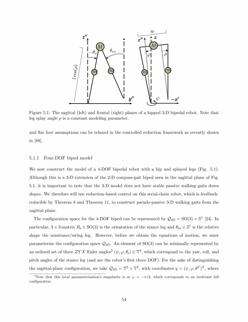
z

mm

ρ

w

ϕ

M

m m

M

y00

z00z00

−x0

l cos(ρ)

ψ

−θs θns

Figure 5.1: The sagittal (left) and frontal (right) planes of a hipped 3-D bipedal robot. Note thatleg splay angle ρ is a constant modeling parameter.

and flat foot assumptions can be relaxed in the controlled reduction framework as recently shown

in [89].

5.1.1 Four-DOF biped model

We now construct the model of a 4-DOF bipedal robot with a hip and splayed legs (Fig. 5.1).

Although this is a 3-D extension of the 2-D compass-gait biped seen in the sagittal plane of Fig.

5.1, it is important to note that the 3-D model does not have stable passive walking gaits down

slopes. We therefore will use reduction-based control on this serial-chain robot, which is feedback-

reducible by Theorem 8 and Theorem 11, to construct pseudo-passive 3-D walking gaits from the

sagittal plane.

The configuration space for the 4-DOF biped can be represented by Q4D = SO(3)× S1 [24]. In

particular, 3× 3-matrix Rs ∈ SO(3) is the orientation of the stance leg and θns ∈ S1 is the relative

shape the nonstance/swing leg. However, before we obtain the equations of motion, we must

parameterize the configuration space Q4D. An element of SO(3) can be minimally represented by

an ordered set of three ZY X Euler angles2 (ψ,ϕ, θs) ∈ T3, which correspond to the yaw, roll, and

pitch angles of the stance leg (and are the robot’s first three DOF). For the sake of distinguishing

the sagittal-plane configuration, we take Q4D = T2 × T2, with coordinates q = (ψ,ϕ, θT )T , where

2Note that this local parameterization’s singularity is at ϕ = −π/2, which corresponds to an irrelevant fallconfiguration.

54

ψ is the yaw (or heading), ϕ is the roll (or lean) from vertical, and θ = (θs, θns)T is the vector of

sagittal-plane (pitch) variables as in the 2-D compass-gait model. All other parameters, including

leg splay angle ρ, are held constant.

Given state x = (qT , qT )T , this model’s hybrid control system is

H C 4D :

x = f4D(x) + g4D(x)u x ∈ D4D\G4D

x+ = ∆4D(x−) x− ∈ G4D

.

We derive the continuous dynamics for H C 4D using Lagrangian mechanics from Section 2.1. We

start with Lagrangian function

L4D(q, q) =1

2qTM4D(q)q − V4D(q),

where recursively-cyclic 4× 4 inertia matrix is given by (see Appendix C for term expressions)

M4D(ϕ, θ) =

mψ(ϕ, θ) —– Mψϕθ(ϕ, θ)

| mϕ(θ) Mϕθ(θ)

MTψϕθ(ϕ, θ) MT

ϕθ(θ) Mθ(θ)

.

The potential energy

V4D(ϕ, θ) = Vθ(θ) cos(ϕ)− g

2(2m+M)(w − 2l sin(ρ)) sin(ϕ) (5.1)

contains the planar subsystem potential energy

Vθ(θ) =gl

2cos(ρ)((3m+ 2M) cos(θs)−m cos(θns)). (5.2)

The dynamical equations of motion for the fully actuated walker are then

M4D(q)q + C4D(q, q)q +N4D(q) = B4Du, (5.3)

where C4D and N4D are defined as usual and invertible 4× 4-matrix

B4D =

I2×2 02×2

02×2 Bθ

with Bθ =

1 1

0 −1

.

55

These dynamics are associated with the control system (f4D, g4D) with input u. We model actuator

saturation at torque constant Umax, so the control space is

U4D = u ∈ R4 : |ui| ≤ Umax, ∀i ∈ 1, 4.

In order to appropriately model walking on a flat surface, we introduce a unilateral constraint

function representing the height of the swing foot3:

H4D(q) = l cos(ρ)(cos(θs)− cos(θns)) cos(ϕ)− (w − 2l sin(ρ)) sin(ϕ).

States corresponding to feasible walking are in domain D4D, the subset of TQ4D where this height

is nonnegative. Impact events are triggered by intersections with the guard, G4D ⊂ D4D, where the

height of the swing foot is zero and strictly decreasing (to exclude events associated with scuffing):

G4D =

q

q

∈ D4D : H4D(q) = 0 and H4D =

(∂H4D(q)

∂q

)Tq < 0

. (5.4)

Following the method of [5,90], we derive the reset map associated with perfectly plastic impacts:

∆4D(q, q) =

Γ4Dq

Ω4D(q)q

, (5.5)

where angular velocity map4 Ω4D(q) ∈ R4×4 and angular position map

Γ4D =

I2×2 02×2

02×2 Γθ

with Γθ =

0 1

1 0

.

The signs of w and ρ are flipped at impact to model the change in stance leg. Technically the hybrid

model then has two sets of continuous/discrete phases, but we forgo this caveat for simplicity and

note that hybrid flows corresponding to walking gaits will be 2-periodic.

3The yaw-DOF (coordinate ψ) is about the vertical axis, and thus the height of the foot H4D(q), measured acrossthis vertical axis, is invariant under such rotations.

4This map’s complexity prevents a closed-form symbolic derivation in Mathematica, so this is computed numeri-cally at each impact event.

56

m m

Mt

Mh

l cos(ρ)

z00

y00

lt cos(ρ)

z

mm

ρϕ

Mt

Mh

−x0

z00w/2

l1

l2

l3

l4

l5

i1

i2i3 i4

lr3

ir3

i5

ψ

−θs θns

−θt

Figure 5.2: The sagittal and frontal planes of a 3-D bipedal torso robot, along with itsserial-chain mapping. Note that i2 is a fixed angle interconnection.

5.1.2 Five-DOF torso biped model

We now construct the model of a 5-DOF bipedal robot with a hip, splayed legs, and a torso (Fig.

5.2). Although this is a 3-D extension of the 2-D compass-gait-with-torso biped, the 3-D biped does

not have stable passive walking gaits down slopes. This model is also entirely feedback-reducible,

i.e., the irreducible tree structure is the last DOF.

For the sake of distinguishing the sagittal plane, we represent the configuration space of the

5-DOF biped by Q5D = T2×T3 with coordinates q = (ψ,ϕ, θT )T , where ψ is the yaw (or heading),

ϕ is the roll (or lean) from vertical, and θ = (θs, θt, θns)T is the vector of sagittal-plane (pitch)

variables as in the 2-D model.

This model’s hybrid control system is

H C 5D :

x = f5D(x) + g5D(x)u x ∈ D5D\G5D

x+ = ∆5D(x−) x− ∈ G5D

.

We derive the continuous dynamics for H C 5D starting with Lagrangian function

L5D(q, q) =1

2qTM5D(q)q − V5D(q),

57

where recursively-cyclic 5× 5 inertia matrix is given by (see Appendix C for term expressions)

M5D(ϕ, θ) =

mψ(ϕ, θ) —– Mψϕθ(ϕ, θ)

| mϕ(θ) Mϕθ(θ)

MTψϕθ(ϕ, θ) MT

ϕθ(θ) Mθ(θ)

and potential energy

V5D(ϕ, θ) = −g2

(2m+Mh +Mt)(w − 2l sin(ρ)) sin(ϕ) + Vθ(θ) cos(ϕ) (5.6)

contains the planar subsystem potential energy

Vθ(θ) =g

2(l cos(ρ)((3m+ 2(Mh +Mt)) cos(θs)−m cos(θns)) + 2ltMt cos(θt)). (5.7)

The equations of motion for the fully actuated biped are then

M5D(q)q + C5D(q, q)q +N5D(q) = B5Du, (5.8)

where C5D and N5D are defined as usual with invertible

B5D =

I2×2 02×3

03×2 Bθ

with Bθ =

1 1 0

0 −1 1

0 0 −1

.

These equations are associated with the control system (f5D, g5D) with input u. We model actuator

saturation at torque constant Umax, so the control space is

U5D = u ∈ R5 : |ui| ≤ Umax, ∀i ∈ 1, 5.

Since the torso does not affect the height of the swing foot, we use the same unilateral constraint

function as before, H5D((ψ,ϕ, θs, θt, θns)T ) = H4D((ψ,ϕ, θs, θns)

T ). States corresponding to feasible

walking are in domain D5D, the subset of TQ5D where this height is nonnegative. Impact events

are triggered by intersections with guard G5D ⊂ D5D, where the height of the swing foot is zero

58

and strictly decreasing:

G5D =

q

q

∈ D5D : H5D(q) = 0 and H5D =

(∂H5D(q)

∂q

)Tq < 0

. (5.9)

Again deferring the details to [5, 90], we can compute the reset map

∆5D(q, q) =

Γ5Dq

Ω5D(q)q

, (5.10)

where angular velocity map Ω5D(q) ∈ R5×5 and angular position map

Γ5D =

I2×2 02×3

03×2 Γθ

and Γθ =

0 0 1

0 1 0

1 0 0

.

The signs of w and ρ are flipped at impact to model the change in stance leg.

Now that we have described our biped models of interest, we construct a general reduction-based

control law to generate walking gaits.

5.2 Reduction-Based Control Law

Given the multistage controlled reduction result of Theorem 11, the controller is designed to recur-

sively break cyclic symmetries in the special almost-cyclic manner. For a general biped, the inner

loop of the control law shapes the robot’s energy into the 2-almost-cyclic form, and the nested

outer loop plays two roles:

1. Implements passivity-based control on the reduced planar subsystem to construct robust gaits

on flat ground.

2. Renders exponentially attractive surface Z defined by constraints (4.2) so that Theorem 10

holds.

We present this control law for a general n-DOF biped, building upon the construction of the

single-stage control law from [46]. As mentioned earlier, we will model actuator saturation to

demonstrate this method’s practicality. We ignore saturation during the control law derivation,

59

but simulations will show that it is indeed robust to clipping effects. We begin by describing the

Lagrangian-shaping inner loop.

5.2.1 Inner loop

We adopt the Lagrangian-shaping control law (4.8) to transform the system Lagrangian into a

2-ACL for controlled reduction to the planar subsystem. As seen in (5.1) and (5.6), the n-DOF

potential energy V is not cyclic in the second variable ϕ, so we impose a “controlled symmetry”

with respect to the second coordinate’s rotation group S1 [24]. This is most naturally accomplished

with potential shaping to replace V with the planar biped’s cyclic potential energy, Vθ (e.g., (5.2)

or (5.7)), constructed from a scaled height due to leg splay. We will incorporate this shaping into

the inner loop, and later revisit another form of controlled symmetry in the outer loop to achieve

slope invariance.

We begin with the 2-ACL of (4.1) for k = 2:

Lλ21(q, q) =1

2qTMλ21

(qn2 )q +QTλ21(q)q − Vλ21(q), (5.11)

where Mλ21, Qλ21 , and Vλ21 are defined in (4.4)-(4.6), substituting Vθ for VRλ . Direct calculation

shows that the stage-2 functional Routhian associated with 2-ACL Lλ21 is the Lagrangian of the

scaled planar walker:

Lθ(θ, θ) =1

2θTMθ(θ)θ + Vθ(θ), (5.12)

which yields the reduced control system (fθ, gθ) with subsystem input vθ.

Given this target reduction, the feedback control law that shapes L into Lλ21 is

u := B−1(C(q, q)q +N(q) +M(ϕ, θ)Mλ21

(ϕ, θ)−1(−Cλ21(q, q)q −Nλ21

(q) +Bv))

, (5.13)

where Cλ21 and Nλ21= ∂

∂qVλ21 are the shaped terms as in (4.8), and the vector v = (vψ, vϕ, vTθ )T

contains the auxiliary control inputs of the outer loop, to be defined later. Finally, using conserved

momentum functions λ1(ψ) = −α1(ψ− ψ) and λ2(ϕ) = −α2ϕ, for α1, α2 > 0, we establish steering

control to constant angle ψ in the yaw/heading DOF and lateral correction to vertical in the

60

roll/lean DOF. Inputting (5.13) into biped control system (f, g), we have the shaped dynamics

Mλ21(ϕ, θ)q + Cλ21(q, q)q +Nλ21

(q) = Bv, (5.14)

which project onto the target dynamics of the scaled planar biped by Theorem 10. We associate

the full-order shaped dynamics with the new control system (fλ21 , gλ21) as in Section 3.2, with outer

loop input v to be defined next.

5.2.2 Outer loop

In order to enforce constraint (4.2) for the decoupling of fθ provided by Theorem 10, we use control

law (4.11) as input v21 to render Z exponentially attractive. The robot’s sagittal plane (the reduced

subsystem) is decoupled along this surface, so we control it as a planar biped with well-known

passivity-based techniques in vθ. The first of these techniques is that of slope-changing “controlled

symmetries,” which will allow our biped to walk on flat ground given planar walking cycles down

slopes [23,24,39].

In three dimensions, the orientation of the ground (the slope) can be represented by a rotation

of the world frame, i.e., an element of SO(3). Thus, any change of slope is characterized by a group

action of SO(3) on the biped’s configuration space Q. If we measured our 4-DOF biped’s joint

angles with respect to relative axes, the group action for any A ∈ SO(3) would be

ΦA(Rs, θns) = (A ·Rs, θns),

or, for the 5-DOF biped,

ΦA (Rs, (θt, θns)) = (A ·Rs, (θt, θns)) .

The behavior of a passive biped strongly depends on the ground slope. Although both the kinetic

energy and impact equations are invariant under the slope changing action Φ, this is not the case

for the potential energy [24]. We can, however, control the robot’s potential to the desired world

orientation and thus impose symmetry on the system, i.e., a controlled symmetry. Any stable limit

cycle down a slope can then be mapped to a stable limit cycle on an arbitrary slope.

For the planar two-link compass-gait biped, stable passive limit cycles exist down shallow slopes

61

between about 3 and 5, as shown in [3,4,9]. The compass-gait-with-torso biped also has passive

walking gaits after applying a PD control law (e.g., a spring-damper) to stabilize the torso upright

[38]. Since we measure our sagittal-plane joint angles with respect to fixed axes as shown in Figs.

5.1-5.2, the group action for either planar robot simplifies to ΦA(θ) = θ+β, where β = σ−γ is the

angle of rotation parameterizing A ∈ SO(2), σ is the slope angle yielding the desired passive limit

cycle (such as π/50), and γ is the actual ground slope angle for controlled “pseudo-passive” walking.

Therefore, we implement controlled symmetries on this sagittal-plane subsystem to generate limit

cycles on flat ground (γ = 0) using control law

vβθ (θ) := B−1θ

∂

∂θ(Vθ(θ)− Vθ(θ + β)) . (5.15)

We can then invoke the main result of [24] in the following:

Theorem 12. Let η : [0, T ] → TQθ be a periodic hybrid flow of planar hybrid control system

H C θ with continuous dynamics E L θ(Lθ) = vθ for vθ = 0 (i.e., a passive hybrid limit cycle).

Then, letting vθ = vβθ (θ) from (5.15), ΦA η : [0, T ] → TQθ is a periodic hybrid flow of the

closed-loop system (i.e., a pseudo-passive hybrid limit cycle).

Similarly, the overall subsystem control law for the 5-DOF biped is

vθ = vβθ (θ) + vpd(θ, θ)

= vβθ (θ) +B−1θ

(0 −kp(θt + β)− kdθt 0

)T, (5.16)

with proportional-derivative gains kp, kd > 0, respectively, to upright the torso. Note, however,

that Theorem 12 does not necessarily hold in the planar subsystems of our 3-D bipeds due to

out-of-plane coupling in the impact equations. This subsystem mapping is instead approximate,

which we will find sufficient for building full-order gaits on flat ground.

These coupled impact equations also amplify state perturbations in several dimensions, having

implications for the robustness of the desired subsystem limit cycle. This is critically important for

steering motions, which inherently deviate from straight-ahead limit cycles. In order to increase

overall robustness, we implement passivity-based reference energy tracking from [36] on the 4-DOF

biped’s planar subsystem, which has nearly constant energy in the hipped 4-DOF case. Note that

the torso’s PD-controller for the 5-DOF model results in non-trivial energy variation, preventing the

application of this form of passivity-based control. We omit the time-varying case of passivity-based

62

energy tracking from [91,92], which has not proven significantly beneficial [92].

To begin, we define the Lyapunov-like storage function

S(θ, θ) =1

2(Hθ(θ, θ)−Hrefθ )2 ≥ 0,

where Hrefθ is constant and Hθ is the planar subsystem energy after imposing controlled symmetry:

Hθ = Kθ + Vβθ (5.17)

= Kθ + Vθ + (−Vθ + Vβθ ),

with Kθ = 12 θTMθ(θ)θ and Vβθ = Vθ(θ + β).

Due to the passivity property of robots, we have

Hθ = θT

(Bθvθ −

∂Vθ∂θ

+∂Vβθ∂θ

)

along trajectories of the shaped system. And, applying passivity-based control

vθ = vβθ + vθ

= B−1θ

(∂Vθ∂θ− ∂Vβθ

∂θ

)+ vθ, (5.18)

on the 2-D subsystem, it follows that Hθ = θT vθ. Then, taking the derivative of the storage

function yields S = (Hθ −Hrefθ )θT vθ.

If we wisely choose the auxiliary input vθ for energy tracking, such as feedback law

vθ(θ, θ) := −B−1θ p(Hθ −Hrefθ )θ (5.19)

with p > 0, then we have the negative semidefinite storage rate

S = −2p||θ||2S ≤ 0.

It is proven in [36] that under reasonable conditions (including control input saturation), this

implies exponential convergence of a planar biped’s total energy to the reference energy between

step impacts. If the reference is chosen to be the constant energy corresponding to a stable limit

63

Table 5.1: 4-DOF Biped Model Parameters

Physical Hip Mass Leg Mass Hip Width Leg Length Leg Splay Saturation

Variable M m w l ρ Umax

Value 10 kg 5 kg 0.1 m 1 m 0.0188 rad 20 Nm

Control λ1-gain λ1-angle λ2-gain h1-gain h2-gain vβθ -angle vθ-gain vθ-energy

Variable α1 ψ α2 ξ1 ξ2 β p HrefθValue 15 0 rad 10 30 15 π/50 rad 20 154.8742 J

cycle (assuming that the limit cycle has nearly constant energy), then this passivity-based controller

expands the limit cycle’s basin of attraction.

The subsystem control law (5.16) or (5.18) for the 4-DOF or 5-DOF biped, respectively, is

incorporated into the full-order shaped system (fλ21 ,gλ21) by defining the new control system (fλ21 ,gλ21)

with input v21 = (vψ, vϕ)T as in (3.23). The controlled 2-reduced vector field fθ is defined by (3.26).

5.3 Four-DOF Biped Simulations

We now examine our 4-DOF biped, introduced in Section 5.1, with physical parameters shown

in Table 5.1. In order to walk straight-ahead using reduction-based control law (5.13), we choose

momentum function λ1 with gain constant α1 = 15 and desired heading ψ = 0 to counteract the

yaw motion induced by the hip. The other control parameters are given in Table 5.1. Applying

(5.13) under saturation constant Umax = 20 Nm, the hybrid control system H C 4D yields the

closed-loop hybrid system H cl4D for the controlled reduction depicted in Fig. 5.3.

Generally speaking, we cannot analyze the stability of H cl4D using the restricted Poincare map

associated with the planar subsystem. We cannot invoke Theorem 4 to show stability of the divided

coordinates a priori, because joint velocities encounter a discontinuous jump off the conserved

quantity surface Z4D at every impact event (except for the special case of hipless bipeds studied

in [45] and [51]). Away from this surface, solutions of fλ21 and fθ cannot be analytically related by

Theorem 10, so the beneficial decoupling effect for the planar limit cycle does not hold.

We tune the output linearizing control law v21 with sufficiently large gains ξ1, ξ2 to quickly correct

this error during each step cycle, so that any perturbed trajectory does not leave the basin of

attraction of the subsystem limit cycle (which is expanded by passivity-based law vθ). We can then

numerically verify stability of the full-order biped walking straight-ahead on flat ground.

64

4-DOF 3D biped(no stable gaits)

4-DOF 3D biped with LES gaits

3-DOF 3D biped with LES gaits

2-DOF planar biped with LES gaits

energy shaping control

MM

mmm mmmll

zz

yy

ssnsns

reduction (yaw)controlled

reduction (roll)controlled

Figure 5.3: Controlled reduction overview of 4-DOF biped: the first reduction stage divides outthe yaw DOF of the transverse plane, and the second stage divides out the lean DOF of thefrontal plane, yielding the dynamics of the planar 2-DOF compass-gait biped.

5.3.1 Straight-ahead walking

Simulations in Matlab show that H cl4D produces a 2-periodic hybrid orbit, O4D of Fig. 5.4, which is

constructed from its planar subsystem’s hybrid orbit. The intersection between O4D and Poincare

section G4D over two steps is the 2-fixed point

x∗ ≈ (0.0699, 0.0135,−0.3074, 0.3102, 0.0774,−0.0508,−1.6907,−2.0610)T .

We numerically calculate the eigenvalue magnitudes of the linearized Poincare map δP 24D about

this 2-fixed point to be within the unit circle:

|eigx∗| ≈ 0.2047, 0.2047, 0.1286, 0.0383, 0.0037, 0.0000, 0.0000, 0.0000 ,

thus confirming that O4D is LES. We see in Fig. 5.4 that the yaw dynamics of the transverse

plane and the lean dynamics of the frontal plane follow 2-periodic hybrid orbits. These motions

are naturally induced by the robot’s hip during each step cycle (and we verify that these motions

disappear when w = 0, ρ = 0), but evolve in a controlled periodic manner due to our choice of

conserved momentum functions.

At the perfectly plastic impact events, the swing foot’s velocity component normal to ground

is instantaneously dissipated, resulting in a discontinuous loss of total stored (unshaped) energy.

65

−0.50

0.5

−4.5−4

−3.5−3

−2.5−2

−1.5−1

−0.50

0

0.2

0.4

0.6

0.8

−0.4 −0.3 −0.2 −0.1 0 0.1 0.2 0.3 0.4 0.5−2.5

−2

−1.5

−1

−0.5

0

0.5

1

1.5

2

2.5

Angular position [rad]

Ang

ular

vel

ocity

[rad

/sec

]

(ψ, ψ) (ϕ, ϕ) (θs, θs) (θns, θns)

0 0.5 1 1.5−0.4

−0.3

−0.2

−0.1

0

0.1

0.2

0.3

0.4

0.5

Time [sec]

Ang

ular

pos

ition

[rad

]

ψ ϕ θs θns

0 0.5 1 1.5−20

−15

−10

−5

0

5

10

15

20

Time [sec]

Con

trol

Tor

ques

[Nm

]

uψ uϕ uθs uθns

0 0.5 1 1.5−1

−0.8

−0.6

−0.4

−0.2

0

0.2

0.4

0.6

0.8

1

Time [sec]

Ang

ular

vel

ocity

[rad

/sec

]

hϕ = ϕactual − ϕdesired

hψ = ψactual − ψdesired

Figure 5.4: 4-DOF biped’s 2-periodic straight-ahead gait animation (top), phase portrait (middleleft), joint trajectory (middle right), saturated control (bottom left), and conserved quantityerrors (bottom right). The phase portrait shows planar slices of O4D by plotting angular positionsagainst angular velocities, illustrating 2-step periodicity in the phase space.

66

0 0.5 1 1.50.4

0.6

0.8

1

1.2

1.4

1.6

1.8

2

2.2

2.4

Time [sec]

Spe

cific

pow

er [W

/kg]

0 0.5 1 1.5150

151

152

153

154

155

156

157

158

159

Time [sec]

Tot

al e

nerg

y [J

]

0 0.5 1 1.50

50

100

150

200

250

Time [sec]

Ver

tical

gro

und

reac

tion

forc

e [N

]

0 0.5 1 1.50

0.1

0.2

0.3

0.4

0.5

0.6

0.7

0.8

0.9

1

Time [sec]

Sta

tic C

oulo

mb

fric

tion

ratio

Frontal |Fx/Fz|Sagittal |Fy/Fz|

Figure 5.5: Characteristics of 4-DOF biped’s 2-periodic straight-ahead gait: instantaneousspecific power (top left), total stored energy (top right), vertical ground reaction force (bottomleft), and Coulomb friction ratios (bottom right).

We see in Fig. 5.5 that this loss is gradually replenished by controlled symmetries law (5.15) as

the virtual gravity vector accelerates the biped between impact events. However, the clipped input

spikes (Fig. 5.4) and corresponding impulses in instantaneous power qT τ (Fig. 5.5) are artifacts of

subcontrollers (5.18) and (4.11) acting to proportionally correct the error in conserved quantities

and planar-subsystem energy, respectively, introduced by each impact discontinuity. These spikes

might raise concern about violating contact constraints at the stance foot, but we can show that

our choice of input saturation enforces these constraints.

5.3.2 Contact constraints

This simulation uses a model of a kinematic chain with its base fixed at the contact point between

stance foot and ground. However, bipedal locomotion is unilaterally constrained in the vertical

contact force: the robot’s foot can only exert a negative force against ground, resulting in an equal

and opposite (positive) reaction force. When this vertical ground reaction force (GRF) becomes

zero, the robot loses contact with ground and begins a flight phase, which would violate our fixed-

67

base assumption. We must satisfy another contact constraint to prevent slipping: the ratio of

each horizontal GRF component to the vertical GRF component remains smaller than the static

Coulomb friction coefficient [93], i.e., the GRF vector remains inside the friction cone.

We therefore calculate the GRF vector Fext = (Fx, Fy, Fz)T needed to keep the stance foot fixed

at this ground contact point throughout the 4-DOF walking gait, and verify the two conditions

needed for the validity of the above simulation:

1. The vertical GRF component remains strictly positive, i.e., Fz(t) > 0 for all t.

2. The GRF vector remains within the friction cone, i.e., |Fx(t)/Fz(t)|, |Fy(t)/Fz(t)| < µ for all

t with static Coulomb friction coefficient µ = 1 (provided by rubber feet).

This requires us to model an extended (n+3)-DOF system with generalized configuration vector

qe = (qTpos, qT )T , where qpos = (xpos, ypos, zpos)

T ∈ R3 is the Cartesian coordinate vector for the

stance ankle. Therefore, system (5.3) with a floating base at the stance ankle becomes

M e4D(qe)qe + Ce

4D(qe, qe)qe +N e4D(qe) = Be

4Du+

(Fext

0n×1

), (5.20)

Applying saturated control law (5.13), we have the closed-loop system with extended state xe =(qeqe

):

xe = fe(xe) + ge(xe)Fext. (5.21)

Following the derivation from [5], we define output vector ye = he(xe) := qpos, which must be

identically zero to satisfy the contact constraints:

he = Lfehe + (Lgehe)Fext ≡ 0, (5.22)

where Lie derivative Lgehe = ∇xehege = 0. Taking the next time-derivative,

he = L2fehe + LgeLfeheFext ≡ 0 (5.23)

=⇒ Fext = −(LgeLfehe)−1L2

fehe, (5.24)

where LgeLfehe is the (invertible) top-left 3× 3 submatrix of M e−1

4D and L2fehe = [I3×3 03×n] fe.

The vertical GRF component Fz is plotted through the 4-DOF walking gait in Fig. 5.5, verifying

strict positivity. The Coulomb friction ratios |Fx(t)/Fz(t)| and |Fy(t)/Fz(t)| are also shown to

68

be within the friction cone limits for rubber feet. We have confirmed the validity of the above

simulations, and we similarly verify these conditions for the remaining simulations in this thesis.

5.3.3 Robustness to perturbations

We examine gait robustness by perturbing the 2-fixed point corresponding to the biped with

passivity-based energy tracking (gain p = 20) and the biped without passivity-based energy track-

ing (gain p = 0). Using perturbations δq = 0.01, δq = 0.05, we simulate six steps and observe

the response for each system. We see in the state trajectories of Fig. 5.6 that the walker begins

to fall without energy tracking but recovers nicely with the passivity-based control. Moreover,

the energy plots show that the former system is unable to contain the subsystem energy after the

perturbation (leading to instability), but the passivity-controlled system sufficiently insulates the

subsystem energy and allows convergence to the limit cycle. In general, we observe that limit cycle

convergence takes far fewer steps when using the passivity-based energy-tracking subcontroller.

5.3.4 Steering

This inherent robustness is also useful for attenuating perturbations from steering, which enter

the system as changes in heading set-point ψ of control law (5.13). In particular, we instruct the

4-DOF biped to perform a 90 turn over several steps as in the human steering study of [94, 95].

Starting with ψ = 0, a simple event-based supervisory controller increments this desired heading

every other step by steering angle s = δψ = π/10 until ψ = π/2. The turning maneuver, phase

portrait, joint trajectories, saturated torques, and conserved quantity errors are shown in Fig. 5.7.

We see that the zero dynamics subcontroller corrects the conserved quantities between each step.

The passivity-based control keeps the sagittal subsystem energy Hθ at the desired level, despite the

injected energy from yaw rotation. Once the biped meets desired heading ψ = π/2, its gait stably

converges to the straight-ahead 2-periodic limit cycle of O4D with a horizontally-shifted yaw orbit.

Since turning motions inherently deviate from straight-ahead limit cycles, we say for now that the

biped is robust to this sequence of steering angles. We return to the notion of steering stability in

Sections 5.4.2 and 6.3.

69

−0.4 −0.3 −0.2 −0.1 0 0.1 0.2 0.3 0.4 0.5 0.6−4

−3

−2

−1

0

1

2

3

Angular position [rad]

Ang

ular

vel

ocity

[rad

/sec

]

(ψ, ψ) (ϕ, ϕ) (θs, θs) (θns, θns)

−0.4 −0.3 −0.2 −0.1 0 0.1 0.2 0.3 0.4 0.5 0.6−4

−3

−2

−1

0

1

2

3

Angular position [rad]

Ang

ular

vel

ocity

[rad

/sec

]

(ψ, ψ) (ϕ, ϕ) (θs, θs) (θns, θns)

0 0.5 1 1.5 2 2.5 3 3.5 4 4.5−0.4

−0.3

−0.2

−0.1

0

0.1

0.2

0.3

0.4

0.5

0.6

Time [sec]

Ang

ular

pos

ition

[rad

]

ψ ϕ θs θns

0 0.5 1 1.5 2 2.5 3 3.5 4 4.5−0.4

−0.3

−0.2

−0.1

0

0.1

0.2

0.3

0.4

0.5

0.6

Time [sec]

Ang

ular

pos

ition

[rad

]

ψ ϕ θs θns

0 0.5 1 1.5 2 2.5 3 3.5 4 4.5152

153

154

155

156

157

158

159

160

161

162

Time [sec]

Sag

ittal

−pl

ane

ener

gy [J

]

0 0.5 1 1.5 2 2.5 3 3.5 4 4.5152

153

154

155

156

157

158

159

160

161

162

Time [sec]

Sag

ittal

−pl

ane

ener

gy [J

]

Figure 5.6: Perturbation responses of 4-DOF biped with passivity-based energy tracking (left)and without (right): phase portrait (top), joint trajectories (middle), and planar-subsystemenergy trajectory (bottom).

70

0.5 1 1.5 2 2.5 3 3.5

−3

−2

−1

0

0

0.5

1

−0.4 −0.2 0 0.2 0.4 0.6 0.8 1 1.2 1.4 1.6−3

−2

−1

0

1

2

3

Angular position [rad]

Ang

ular

vel

ocity

[rad

/sec

]

(ψ, ψ)

(ϕ, ϕ)

(θs, θs)

(θns, θns)

0 1 2 3 4 5 6 7 8−0.4

−0.2

0

0.2

0.4

0.6

0.8

1

1.2

1.4

1.6

Time [sec]

Ang

ular

pos

ition

[rad

]

ψ ϕ θs θns

0 1 2 3 4 5 6 7 8−20

−15

−10

−5

0

5

10

15

20

Time [sec]

Con

trol

Tor

ques

[Nm

]

uψ uϕ uθs uθns

0 1 2 3 4 5 6 7 8−2

−1.5

−1

−0.5

0

0.5

Time [sec]

Ang

ular

vel

ocity

[rad

/sec

]

hϕ = ϕactual − ϕdesired

hψ = ψactual − ψdesired

Figure 5.7: 4-DOF biped’s 90-turning maneuver’s animation (top), phase portrait (middle left),joint trajectory (middle right), saturated control (bottom left), and conserved quantity errors(bottom right).

71

Table 5.2: 5-DOF Biped Model Parameters

Physical Hip Mass Leg Mass Hip Width Leg Length Leg Splay

Variable Mh m w l ρ

Value 10 kg 5 kg 0.1 m 1 m 0.0188 rad

Physical Cont’d Torso Mass Torso Length Saturation

Variable Mt lt Umax

Value 10 kg 0.5 m 30 Nm

Control λ1-gain λ1-angle λ2-gain h1-gain h2-gain vpd-gain vpd-gain vβθ -angle

Variable α1 ψ α2 ξ1 ξ2 kp kd β

Value 20 0 rad 30 30 15 700 200 0.052 rad

5.4 Five-DOF Biped Simulations

After applying feedback control law (5.13) under actuator saturation, closed-loop hybrid system

H cl5D, with physical and control parameters in Table 5.2, provides the controlled reduction depicted

in Fig. 5.8. As was the case with the 4-DOF biped, we cannot analyze the stability of H cl5D using

the restricted Poincare map associated with the reduced subsystem. We will show, however, that

H cl5D is similarly robust to brief errors off Z5D by considering the biped’s full-order behavior.

5.4.1 Straight-ahead walking

When walking straight-ahead on flat ground, H cl5D produces a 2-step periodic orbit, Ost

5D of Fig.

5.9, which is constructed from its planar subsystem’s limit cycle. The intersection between Ost5D

and Poincare section G5D is the 2-fixed point

x∗st ≈ (0.0544, 0.0062,−0.2543, 0.0021, 0.2558, 0.0673,−0.0173,−1.2871, 0.0673,−1.7233)T .

We numerically calculate the eigenvalues of the linearized Poincare map δP 25D about this fixed-point

over two steps:

|eigx∗st| ≈ 0.7629, 0.7629, 0.2745, 0.0736, 0.0344, 0.0134, 0.0034, 0.0003, 0.0003, 0.0000 .

All magnitudes are within the unit circle, thus confirming LES. We also see that the yaw and lean

dynamics follow 2-periodic orbits, a natural result of the controlled reduction.

72

5-DOF 3D biped(no stable gaits)

5-DOF 3D biped with LES gaits

4-DOF 3D biped with LES gaits

3-DOF planar biped with LES

gaits

reduction (yaw)

energy shaping control

controlled

reduction (roll)controlledmmm mmm

MtMtMM

MhMhMM

ll

ltlt

yy

zz

ssnsns

tt

Figure 5.8: Controlled reduction overview of 5-DOF biped: the first reduction stage divides outthe yaw DOF of the transverse plane, and the second stage divides out the lean DOF of thefrontal plane, yielding the dynamics of the planar 3-DOF compass-gait-with-torso biped.

5.4.2 Steering

We demonstrate steering capabilities with the 90 turning maneuver seen in Fig. 5.10. Starting

with ψ = 0, an event-based supervisory controller increments this desired yaw angle every other

step by steering angle s = δψ = π/14 until ψ = π/2. Once the biped meets this heading, its gait

stably converges to the straight-ahead limit cycle of Ost5D with a horizontally-shifted yaw orbit.

If we instead continue this constant-curvature steering, we observe convergence to a periodic

turning gait modulo yaw :

x∗tu(s) + (s 01×9)T = P 2tu(s)

(x∗tu(s)

),

where the 2-fixed point of orbit Otu(s)5D is given by

x∗tu(s) ≈ (0.2147, 0.0185,−0.2534, 0.0043, 0.2488, 0.0015,−0.0052,−1.2706, 0.0601,−1.7303)T .

This orbit is confirmed LES (modulo s) with eigenvalues

|eigx∗tu(s)| ≈ 0.7835, 0.3594, 0.2111, 0.2111, 0.0386, 0.0047, 0.0047, 0.0003, 0.0001, 0.0000 .

73

−0.4−0.20 0.2

−4

−3.5

−3

−2.5

−2

−1.5

−1

−0.5

0

0

0.5

1

−0.3 −0.2 −0.1 0 0.1 0.2 0.3 0.4 0.5−2

−1.5

−1

−0.5

0

0.5

1

1.5

2

Angular position [rad]

Ang

ular

vel

ocity

[rad

/sec

]

(ψ, ψ)

(ϕ, ϕ)

(θs, θs)

(θt, θt)

(θns, θns)

0 0.2 0.4 0.6 0.8 1 1.2 1.4 1.6−0.3

−0.2

−0.1

0

0.1

0.2

0.3

0.4

0.5

Time [sec]

Ang

ular

pos

ition

[rad

]

ψ ϕ θs θt θns

0 0.2 0.4 0.6 0.8 1 1.2 1.4 1.6−30

−20

−10

0

10

20

30

Time [sec]

Con

trol

Tor

ques

[Nm

]

uψ uϕ uθs uθt uθns

0 0.2 0.4 0.6 0.8 1 1.2 1.4 1.6−1.2

−1

−0.8

−0.6

−0.4

−0.2

0

0.2

0.4

0.6

0.8

1

Time [sec]

Ang

ular

vel

ocity

[rad

/sec

]

hϕ = ϕactual − ϕdesired

hψ = ψactual − ψdesired

Figure 5.9: 5-DOF biped’s 2-periodic straight-ahead gait animation (top), phase portrait (middleleft), joint trajectory (middle right), saturated control (bottom left), and conserved quantityerrors (bottom right).

74

0.5 1 1.5 2 2.5 3 3.5 4

−3

−2

−1

0

0

0.2

0.4

0.6

0.8

1

1.2

1.4

−0.3 −0.2 −0.1 0 0.1 0.2 0.3 0.4 0.5−2

−1.5

−1

−0.5

0

0.5

1

1.5

2

Angular position [rad]

Ang

ular

vel

ocity

[rad

/sec

]

(ψ, ψ)

(ϕ, ϕ)

(θs, θs)

(θt, θt)

(θns, θns)

0 0.2 0.4 0.6 0.8 1 1.2 1.4 1.6−0.3

−0.2

−0.1

0

0.1

0.2

0.3

0.4

0.5

Time [sec]

Ang

ular

pos

ition

[rad

]

ψ ϕ θs θt θns

0 0.2 0.4 0.6 0.8 1 1.2 1.4 1.6−30

−20

−10

0

10

20

30

Time [sec]

Con

trol

Tor

ques

[Nm

]

uψ uϕ uθs uθt uθns

0 0.2 0.4 0.6 0.8 1 1.2 1.4 1.6−1.2

−1

−0.8

−0.6

−0.4

−0.2

0

0.2

0.4

0.6

0.8

1

Time [sec]

Ang

ular

vel

ocity

[rad

/sec

]

hϕ = ϕactual − ϕdesired

hψ = ψactual − ψdesired

Figure 5.10: 5-DOF biped’s 2-periodic turning gait animation (top), phase portrait (middle left),joint trajectory (middle right), saturated control (bottom left), and conserved quantity errors(bottom right).

75

We see in Fig. 5.10 that Otu(s)5D has a perturbed subsystem orbit compared to Ost

5D, since the

outer leg swings a longer distance in arclength5 (1.081 m) than the inner leg (1.033 m) along this

curved path. This behavior occurs naturally (without reference trajectories) and resembles the

turning perturbations in the human studies of [94], which we discuss further in Chapter 7. In

general, we find that stable turning gaits exist for a wide range of steering angles, as documented

in [43,50,51]. We show how the 2-fixed-point and gait characteristics of linear step length and time

period evolve over the range of steering angles [0, 0.235] in Fig. 5.11. Beyond this range, we notice

a period-doubling bifurcation leading to chaotic instability, shown in Fig. 5.12.

5.5 Energetic Efficiency

We can analyze the energetic cost of these gaits by integrating qT τ to obtain the net work per step.

In particular, we use this to calculate the specific mechanical cost of transport cmt (mechanical

work done per unit weight per unit distance), which is a dimensionless metric commonly adopted

to study the efficiency of a locomotor control strategy on a given mechanical system [15,96].

We find that the cost of the 4-DOF biped for straight-ahead walking is cmt = 0.073 and for

turning is cmt = 0.071. The cost for the 5-DOF straight-ahead and turning gaits are lower at

cmt = 0.036 and cmt = 0.037, respectively. These numbers are comparable with human walking (in

terms of metabolic cost) at cmt = 0.5 and the Cornell biped at cmt = 0.055, and far surpass Honda

ASIMO at cmt = 1.6 as seen in Fig. 5.13 [15]. The improved efficiency of the 5-DOF gaits over the

4-DOF gaits is attributable to the torso link, which naturally leans into the direction of walking

during substantial portions of the gait. In other words, the torso’s center of mass contributes a

gravitational force to the forward ballistic motion. This is exploited in the optimized gaits of [5,34]

resulting in more exaggerated torso pitch.

We must note, however, that this metric does not account for power consumption of the on-board

control system or the actuators – the energetic cost of transport cet (energy consumed per unit

weight per unit distance) must be computed for this purpose [15]. Since the models presented have

only been studied in simulation, we can only speculate about energetic cost based on the efficiency

(in terms of cmt) of the underlying reduction-based control strategy. A conservative estimate that

assumes fifty percent actuator efficiency with no regeneration during negative work still results in

5Although the outer leg swings a longer distance in arclength than the inner leg for sharp turns, the linear distancebetween step placements has an inverse relationship for large steering angles as seen in Fig. 5.11.

76

0 0.05 0.1 0.15 0.2 0.25−0.3

−0.2

−0.1

0

0.1

0.2

Steering angle [rad]

Fix

ed−

poin

t ang

les

[rad

]

ψ ϕ θs θt θns

0 0.05 0.1 0.15 0.2 0.25−0.9

−0.8

−0.7

−0.6

−0.5

−0.4

−0.3

−0.2

−0.1

0

0.1

Steering angle [rad]

Fix

ed−

poin

t ang

ular

vel

ociti

es [r

ad/s

]

ψ ϕ θs θt θns

0 0.05 0.1 0.15 0.2 0.250.04

0.06

0.08

0.1

0.12

0.14

0.16

0.18

Steering angle [rad]

x−ax

is d

ispl

acem

ent [

m]

0 0.05 0.1 0.15 0.2 0.250.995

1

1.005

1.01

1.015

1.02

1.025

1.03

1.035

Steering angle [rad]

y−ax

is d

ispl

acem

ent [

m]

0 0.05 0.1 0.15 0.2 0.250.49

0.5

0.51

0.52

0.53

0.54

Steering angle [rad]

Line

ar s

trid

e le

ngth

[m]

Inner LegOuter Leg

0 0.05 0.1 0.15 0.2 0.250.71

0.72

0.73

0.74

0.75

0.76

0.77

0.78

0.79

0.8

0.81

Steering angle [rad]

Ste

p tim

e pe

riod

[s]

Inner LegOuter Leg

Figure 5.11: Evolution of 5-DOF biped’s turning 2-fixed-point x∗tu(s) (top), x-axis displacement(middle left), y-axis displacement (middle right), linear step length (bottom left), and step timeperiod (bottom right) over steering angle s ∈ [0, 0.235].

0.235 0.245 0.255 0.265 0.275 0.285 0.2910.47

0.48

0.49

0.5

0.51

0.52

0.53

0.54

0.55

0.56

Steering angle [rad]

Line

ar s

trid

e le

ngth

[m]

Inner LegOuter Leg

0.235 0.245 0.255 0.265 0.275 0.285 0.2910.6

0.65

0.7

0.75

0.8

0.85

Steering angle [rad]

Ste

p tim

e pe

riod

[s]

Inner LegOuter Leg

Figure 5.12: Bifurcation diagram of 5-DOF biped’s linear step length (left) and time period(right) over steering angle s ∈ [0.235, 0.2914].

77

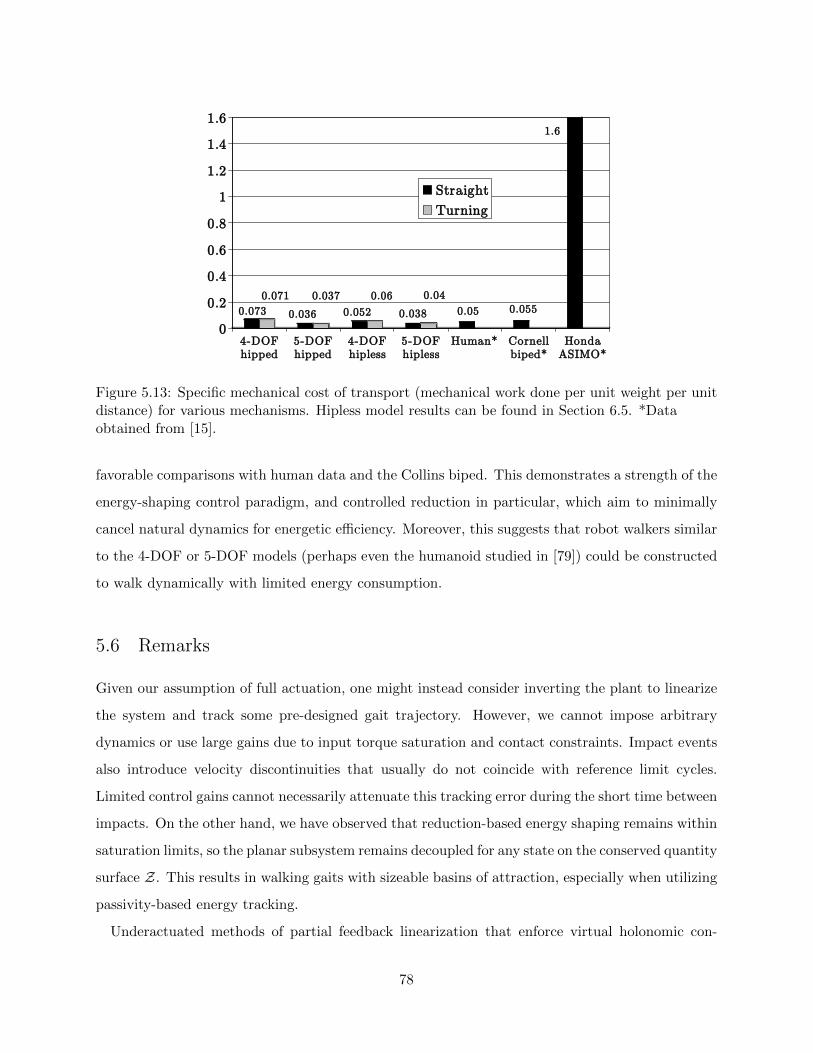
0.073

0.071

0.036

0.037

0.052

0.06

0.038

0.04

0.05 0.055

1.6

0

0.2

0.4

0.6

0.8

1

1.2

1.4

1.6

4-DOFhipped

5-DOFhipped

4-DOFhipless

5-DOFhipless

Human* Cornellbiped*

HondaASIMO*

Straight

Turning

Figure 5.13: Specific mechanical cost of transport (mechanical work done per unit weight per unitdistance) for various mechanisms. Hipless model results can be found in Section 6.5. *Dataobtained from [15].

favorable comparisons with human data and the Collins biped. This demonstrates a strength of the

energy-shaping control paradigm, and controlled reduction in particular, which aim to minimally

cancel natural dynamics for energetic efficiency. Moreover, this suggests that robot walkers similar

to the 4-DOF or 5-DOF models (perhaps even the humanoid studied in [79]) could be constructed

to walk dynamically with limited energy consumption.

5.6 Remarks

Given our assumption of full actuation, one might instead consider inverting the plant to linearize

the system and track some pre-designed gait trajectory. However, we cannot impose arbitrary

dynamics or use large gains due to input torque saturation and contact constraints. Impact events

also introduce velocity discontinuities that usually do not coincide with reference limit cycles.

Limited control gains cannot necessarily attenuate this tracking error during the short time between

impacts. On the other hand, we have observed that reduction-based energy shaping remains within

saturation limits, so the planar subsystem remains decoupled for any state on the conserved quantity

surface Z. This results in walking gaits with sizeable basins of attraction, especially when utilizing

passivity-based energy tracking.

Underactuated methods of partial feedback linearization that enforce virtual holonomic con-

78

straints rather than reference trajectories have been successful on 3-D bipeds with unactuated

ankles [34,35]. Although controlled reduction requires actuation at the stance ankle, the yaw DOF

input could be realized mechanically with a passive damper as shown in Section 3.2. This would

allow a more feasible (and arguably anthropomorphic) implementation with a 2-DOF ankle actu-

ator for lean and pitch – humans routinely actuate these DOFs during walking and certainly have

passive yaw damping through ankle tendons and/or rotational friction when pivoting about the

ground contact point. In fact, peak power output during a human walking gait occurs at the ankle

pitch DOF during push-off [97], which we observe in our reduction-based results (with the caveat

that double-support is instantaneous so push-off appears to occur immediately at impact).

We have shown that increasingly complex bipedal robots can achieve stable directional 3-D

walking with reduction-based control. This method embraces the beneficial passive dynamics of

the robot in order to produce time-invariant and asymptotically stable walking with human-like

swaying motion. This provides robustness to small perturbations (e.g., steering), naturally resulting

in multiple types of dynamic walking gaits. We next show that these straight-ahead and turning

gaits form a set of motion primitives for planning stable walking paths through 3-D environments.

79

CHAPTER 6

GAIT PRIMITIVES FOR MOTION PLANNING

We saw in the previous chapter that reduction-based control yields directional control authority

to produce asymptotically stable turning gaits. Related results for underactuated 3-D bipeds are

presented in [35], where virtual constraints are enforced to restrict analysis to the periodic motion

of a reduced-order subsystem. Both methods demonstrate steering capabilities, with the latter

showing input-to-state stability for steering along paths with sufficiently mild curvature.

In order to build bipedal robots that can quickly and efficiently navigate through real-world

environments, the stability of dynamic walking must be considered when planning walking paths

with significant steering. Therefore, we present in this chapter the motion planning framework

of [43,98] for bipeds that exhibit asymptotically stable (i.e., dynamic) walking behavior. We show

that straight-ahead and turning gaits form a set of gait primitives that can be sequentially composed

under bounded curvature and switching conditions without causing the biped to fall. This employs

a discrete-time analogy of the switching controller-composition method of [52], where (Lyapunov)

funnels show stability for sequential paddle-and-ball batting maneuvers.

6.1 Quasi-Static Motion Planning

We begin by reviewing some motivating work in humanoid path planning based on primitives

satisfying postural ZMP constraint (1.4). Note, however, the important distinction that satisfying

this ZMP condition does not necessarily imply stable walking motion [6, Section 10.8].

Full-body posture planning is achieved in [19] by initially computing a large set of statically-stable

configurations. A path between goal configurations is then found by growing a rapidly-exploring

random tree, which connects samples only if a collision-free ZMP-constrained path exists. This is

used in [20] for locomotion planning, restricting the problem to a discrete set of foot placements

connected by valid stepping motions. A similar method in [21] pre-computes a small set of ZMP-

constrained motion primitives, which bias the sampling of configurations between planned foot

80

placements. These primitives prescribe high-quality motions that can be shaped to match common

tasks such as for walking and climbing. Instead of tracking pre-computed trajectories, our approach

is based on autonomous LES limit cycles.

A two-stage global planner is proposed in [17] that first uses a sampling-based algorithm to find a

collision-free path for the functional decomposition of the robot body. That is, the robot is modeled

as a bounding box on a walking surface, reducing the initial planning problem to configuration

space SE(2) – x, y position and orientation. Randomly generated samples are locally connected by

Dubins curves (circular arcs with tangential line segments [99]), and these SE(2) paths are given to a

walking pattern generator that produces whole-body motions for ZMP-constrained locomotion. We

will show that the nature of our gait primitives allows a similar functional decomposition approach

for generating stable dynamic walking paths composed of constant-curvature arc segments.

6.2 Asymptotically Stable Gait Primitives

We can now formalize the notion of asymptotically stable gait primitives corresponding to strate-

gies for straight-ahead walking and turning1 clockwise (CW) or counter-clockwise (CCW). These

strategies will enable motion planning for dynamic walkers in 3-D space.

Definition 15. An asymptotically stable gait primitive is a pair G = (P hcl, x∗), where Pcl is a

closed-loop Poincare map for which x∗ is an asymptotically stable h-fixed-point (modulo yaw).

Since asymptotically stable limit cycles are fundamental to dynamic walking, we often call these

dynamic gait primitives for brevity. For the purpose of sequential composition, a gait can be

arbitrarily oriented about the z-axis for walking along any heading:

Proposition 8. Given G = (P hψi, x∗ψi) with steady-state heading ψi and desired heading ψi,

x∗ψj := x∗ψi + (s 02n−1)T

is the LES h-fixed-point of P hψj

with ψj = ψi + s and ψj = ψi + s, for any s ∈ S1.

Moreover, each primitive is independent of world position (this does not appear in state x),

and each closed-loop hybrid system is autonomous (no reference trajectories). In other words, gait

primitives are invariant with respect to time and SE(2) (spatial-temporal symmetry). A general set

1Note that our steering strategies resemble human “spin” turns [100], which we discuss in Chapter 7.

81

of gait primitives Ps = Gst,Gtu(s),Gtu(−s), continuously parameterized by steering angle s = δψ,

can thus be sequentially composed from step to step. Each gait has a nominal walking arc on the

ground plane, with which we can plan walking paths. Switching between the closed-loop hybrid

systems associated with each gait primitive will result in transient variations, so we must first

consider the stability of such transitions.

6.3 Sequential Composition of Gait Primitives

In order to sequentially compose gait primitives in a stable manner, we present a discrete switched

system analogy to the funneling approach of [52]. We consider a set of dynamic gait primitives for

a general biped, where we do not have an analytical/closed-form expression for the Poincare map

between steps.

A biped employs2 gait primitive Gi = (Pi, x∗i ) during step cycle i by implementing the controller

yielding Poincare map Pi associated with closed-loop hybrid system H i. Gait primitives are

selected at every impact event, so every step has an associated gait transition.

Definition 16. The gait transition of step i is defined by pair Ti = (xi,Gi+1), where xi is the state

at the ith impact event and Gi+1 is the gait primitive during step cycle i+ 1. Moreover, Ti is said

to be switching if Gi+1 6= Gi.

Hence, Ti+1 is related to Ti by xi+1 = Pi+1(xi). And, in the case of 2-step periodic gaits,

switching may only occur ever other step, implying Gi+1 = Gi for even i.

Definition 17. A gait transition Ti = (xi,Gi+1) is stable if xi ∈ BoA(x∗i+1), where x∗i+1 is the LES

fixed-point of Pi+1 from gait primitive Gi+1 of step cycle i+ 1.

State xi may be the result of any gait primitive. By invariance of the basin of attraction, if

Gi+1 = Gi and Ti−1 is stable, then Ti is also stable. In order to determine stability for switching

transitions, we first require some properties of “nearby” gait primitives.

Assumption 4. For every s ∈ [−S, S], there exists LES fixed-point x∗tu(s) of Ptu(s) with corre-

sponding BoA(x∗tu(s)). Then, by definition there exists a non-empty open ball of radius rs > 0

about x∗tu(s) such that

B(x∗tu(s), rs) ⊂ BoA(x∗tu(s)).

2Turning gaits are implicity understood to be modulo steering angle s, and we assume that each gait primitive isoriented coincident with the biped’s heading at the preceding gait transition.

82

Moreover, assume x∗tu(s) and rs are continuous functions of s.

Property 1. The turning fixed-point x∗tu(s) converges to straight-ahead fixed-point x∗st = x∗tu(0)

in metric space (R2n, d) as |s| → 0, where d is Euclidean distance. Formally speaking, lim|s|→0 r∗s = 0

for r∗s := d(x∗tu(s), x∗st).

In other words, turning motion more closely resembles straight-ahead motion for smaller steering

angles. We know that turning curvature κ = ±1/R converges to straight-line curvature κ = 0 as

turning radius R → ∞ ⇔ |s| → 0. Thus, Property 1 follows from Assumption 4 by continuity.

Loosely speaking, Property 1 implies the basins of attraction also converge, which we exploit next.

Lemma 7. Given Property 1, there exists positive steering angle S ≤ S such that for all s ∈ [−S, S]:

1. x∗st ∈ BoA(x∗tu(s))

2. x∗tu(s) ∈ BoA(x∗st)

3. x∗tu(−s) ∈ BoA(x∗tu(s))

Proof. [1.1] We first define minimal ball radius r := mins∈[−S,S](rs), positive by compactness of

[−S, S], so

B(x∗tu(s), r) ⊂ B(x∗tu(s), rs) ⊂ BoA(x∗tu(s)),

for all s ∈ [−S, S]. Now, since r > 0 and lim|s|→0 r∗s = 0, ∃ S ≤ S such that r∗s < r for all

s ∈ [−S, S]. Then, x∗st ∈ B(x∗tu(s), r) for all s ∈ [−S, S], and the claim follows.

[1.2] First, by definition of LES, ∃ r∞ > 0 such that B(x∗st, r∞) ⊂ BoA(x∗st). Then, again ∃ Ssuch that r∗s < r∞ for all s ∈ [−S, S]. Hence, x∗tu(s) ∈ B(x∗st, r∞) for all s ∈ [−S, S], and the claim

follows.

[1.3] Recall x∗tu(s) → x∗st as |s| → 0, which means that for each ε/2 > 0, ∃ δ > 0 such that for

all s ∈ [−δ, δ], d(x∗tu(s), x∗st) < ε/2. Then, the triangle inequality shows

d(x∗tu(s), x∗tu(-s)) ≤ d(x∗tu(s), x∗st) + d(x∗tu(-s), x∗st)

< ε.

Hence, if r∗tus := d(x∗tu(s), x∗tu(−s)), then lims→0 r∗tus = 0.

83

Now, denoting each turning ball as B(x∗tu(s), rs), we can define minimal ball radius

r := mins∈[−S,S]

(rs) > 0.

As we saw in 1.1, ∃ S such that r∗tus < r for all s ∈ [−S, S]. Then, x∗tu(−s) ∈ B(x∗tu(s), r) for all

s ∈ [−S, S], and the claim follows. Equivalently, x∗tu(s) ∈ BoA(x∗tu(−s)).

Finally, we can take the minimum of S from each proof to find S for the overall Lemma.

Remark 11. Recall that asymptotic stability implies convergence to fixed-points in infinite time,

but trajectories eventually converge “close enough” to stably switch gaits. Note that in Lemma

7.1, B(x∗tu(s), r) is an open ball so x∗st cannot be on the boundary of BoA(x∗tu(s)). Therefore,

points sufficiently close to x∗st are also contained in BoA(x∗tu(s)). The same holds for the other

three claims in Lemma 7.

Fortunately, we also have exponentially fast convergence to neighborhoods around fixed-points.

Given enough time along a given primitive, the biped’s state will be “funneled” into the basin

of attraction of the next primitive upon switching (e.g., Fig. 1.4). This is called the dwell time,

since the biped can be interpreted as a discrete-time switched system x(i+ 1) = Pσ(i) (x(i)), where

switching signal σ : Z+ → 0, s,−s chooses the primitive (parameterized by steering angle) at

every step. This signal must be constrained to ensure stable composition of primitives, for which

we invoke the main result of this chapter (cf. [101, 102] for analogous results on global stability of

continuous-time switched systems):

Theorem 13. For any s ∈ [−S, S] from Lemma 7, there exists a minimum number of steps N ≥ 1,

i.e., a lower bound on dwell time, such that for all integers k ≥ N :

1. If x ∈ BoA(x∗st), then P kst(x) ∈ BoA(x∗tu(s)).

2. If x ∈ BoA(x∗tu(s)), then P ktu(s)(x) ∈ BoA(x∗st).

3. If x ∈ BoA(x∗tu(s)), then P ktu(s)(x) ∈ BoA(x∗tu(−s)).

Corollary 1. Consider primitive set Ps as in Theorem 13. For any s ∈ [−S, S], there exists a

minimum dwell time N ≥ 1 such that for any integer k ≥ N the following holds: any switching

transition Ti+k that follows a stable transition Ti is also stable.

84

Hence, we can design a supervisory controller to produce a constrained σ(·) for stable path

planning, piecing together straight and curved gait segments such that the turns are not too sharp

or the primitive switches too fast. The steering sharpness must be bounded by steering angle S, a

condition that can be verified in simulation (checking convergence from all fixed-points). However,

minimum dwell time N depends explicitly on each gait primitive’s basin of attraction and rate of

exponential convergence, both of which can only be characterized numerically. It is now possible

to use sum-of-squares programming to find invariant subsets of the basins of attraction [103, 104],

which will enable conservative estimates for lower bounds on dwell time as in [102]. For the purposes

of this thesis, we examine our lower bound using exhaustive simulation in Section 6.5.3. We first

turn our attention to building walking paths from gait primitives.

6.4 Path Planning Formulation

Given these switching rules, we can define stable walking over a path of sequentially composed gait

primitives.

Definition 18. A w-step walking path execution from initial condition x(0) = x0 is defined by the

ordered set E(x0) = (T0, T1, . . . , Tw−1), where T0 = (x0,G1).

Definition 19. A walking path execution E(x0) is robust if all gait transitions Ti are stable.

In other words, the biped is guaranteed not to fall over.

6.4.1 Planning in SE(2)

Recall that state x describes the robot’s motion with respect to its joints. In the context of

path planning, we need to consider the robot’s coordinates with respect to a world frame, i.e., its

Euclidean coordinates on the walking surface. Assuming a flat surface, we need only model the

biped’s (x, y)-position (e.g., measured at the stance foot with respect to some world frame) along

with heading ψ as the global orientation. Hence, every step i has an associated world configuration

ci = (xipos, yipos, ψi)

T ∈ SE(2). The extension of a biped’s discrete state to xei = (xipos, y

ipos, x

Ti )T is

trivial, as the new coordinates are easily updated according to robot kinematics. Through a slight

abuse of notation, we denote a boundary-constrained w-step walking path execution as Ecwc0 (xe0),

where c0 is given by xe0 = (cT0 , ϕ0, θ

T0 , q

T0 )T and cw is given by xe

w = Pw(xew−1

)= (cTw, ϕw, θ

Tw, q

Tw)T .

85

tu(s)

st

tu(-s)

ca

b d

ZMP

i

h

e

f g

Figure 6.1: Directed graph of a discrete maneuver automaton for a biped that cannot stablyswitch directly between left and right turning gaits of large curvature, i.e.,x∗tu(−s) /∈ BoAtu(s)(x

∗tu(s)) for some s such that S < |s| ≤ S. This graph also includeshypothetical edges for transitions to/from quasi-static states of locomotion.

We now have the framework to form paths that stably connect initial and final world config-

urations c0, cf . We can use Corollary 1 to define a class Ccfc0 =Ecwc0 |cw = cf , w ≥ 1

of robust

walking path executions between reachable configurations c0 and cf . Moreover, our finite set of

gait primitives is continuously parameterized by s to allow a (large) continuous reachable set. After

encoding the switching rules into a regular language [105], walking paths can be constructed by a

finite-state machine (i.e., a discrete automaton [106]) that outputs a constrained switching signal

σ(·) to the biped switched system. This so-called maneuver automaton can even accommodate

primitive sets in which the CW and CCW turning primitives cannot be directly composed as in

Fig. 6.1. Hence, the switching rules from Section 6.3 allow stability concerns to be abstracted away

from the planning problem.

6.4.2 Walking arcs

As the biped switches between gaits, step cycle trajectories converge back and forth between

attractive orbits, so we generally do not have a fixed mapping from gait transitions to path arcs.

However, this mapping is very closely approximated with the nominal set of constant-curvature

arcs associated with the gait primitives.

Definition 20. The nominal walking arc of primitive G is the tuple(δx∗pos, δy

∗pos, δψ

∗) ∈ SE(2) of

the gait’s x-axis, y-axis, and heading displacements, respectively, from initial heading ψ = 0.

For the gait primitives we consider, the heading change equals the primitive’s steering angle, i.e.,

s = δψ = δψ∗. In order to sequentially compose walking arcs with different orientations, we rotate

86

M

m ml

z

y

−θs θns

m m

Mt

Mh

l

lt

y

z

−θs θns

−θt

Figure 6.2: The sagittal planes of the standard (left) and torso (right) compass-gait bipeds.

the nominal arc’s x-y coordinate frame with a group action of SO(2) to coincide with the initial

heading ψi of the current gait transition Ti = (xi,Gi+1):

δxi+1pos

δyi+1pos

=

cos(ψi) − sin(ψi)

sin(ψi) cos(ψi)

δx∗i+1pos

δy∗i+1pos

. (6.1)

This enables path planning in SE(2) with a discrete tree transversal of branching factor three, the

cardinality of the primitive set (i.e., the action space). In other words, stable dynamic locomotion

planning reduces to a discrete graph search, where the planning algorithm outputs a sequence

S of steering angles parameterizing gait primitives. Although these walking paths (planned a

priori) may have minor transient drift, periodic re-planning or kinodynamic planning methods

(e.g., [107–109]) would enable reachability of specific goal configurations. We will discuss this in

detail when presenting planned walking results in Section 6.6, but we first must define the primitive

sets for our biped examples.

6.5 Primitives for 3-D Compass-Gait Bipeds

In order to demonstrate the fundamentals of dynamic gait primitives, we slightly deviate from the

complex models presented in Chapter 5 by removing the hip link. In other words, we adopt the

two hipless walkers from [51]: the 4-DOF compass-gait biped and 5-DOF compass-gait-with-torso

biped. These are strict 3-D extensions of the commonly studied planar bipeds in Fig. 6.2. The

87

robots are given the respective control laws from Section 5.2 and are simulated with the respective

parameters in Tables 5.1-5.2, except that hip width w = 0, leg splay angle ρ = 0, slope mapping

angle β = 0.052 rad, and gain p = 0 (no passivity-based energy tracking).

We now derive a set of gait primitives for each model. These gaits will be 1-step periodic

since each leg has identical dynamics without the hip link. We note, however, that this planning

framework is applicable to any set of asymptotically stable h-periodic gaits (not necessarily from

our reduction-based control method).

6.5.1 Straight-ahead gait primitives

The reduction-based control law (5.13) yields closed-loop hybrid systems H st4D and H st

5D for straight-

ahead walking on flat ground. For example, we set ψ = 0 (without loss of generality) and find the

1-fixed-points

x∗st4D ≈ (0, 0,−0.2704, 0.2704, 0, 0,−1.4896,−1.7986)T

x∗st5D ≈ (0, 0,−0.2657, 0.0047, 0.2657, 0, 0,−1.3165, 0.0596,−1.5339)T .

We numerically verify LES of each periodic orbit by linearizing the associated Poincare map, thus

defining the straight-ahead gait primitives Gst4D = (P st

4D, x∗st4D) and Gst

5D = (P st5D, x

∗st5D).

The associated hybrid periodic orbits Ost4D and Ost

5D are illustrated in the plots of Fig. 6.3 and

Fig. 6.4, respectively. We see that these upright gaits have no swaying in lean or yaw (which is to

be expected for hipless bipeds). The 4-DOF sagittal plane has a periodic step length of 0.534 m

and an approximate linear velocity of 0.727 m/s, whereas the 5-DOF sagittal plane has a periodic

step length of 0.525 m and an approximate linear velocity of 0.692 m/s.

6.5.2 Turning gait primitives

We create turning gaits by introducing a periodic disturbance into each biped’s straight-ahead

system H st in the form of constant steering between steps. In particular, we augment the within-

stride reduction-based controller with an event-based (or stride-to-stride) controller that increments

yaw set-point ψ at each step by steering angle s (positive for CW or negative for CCW steering).

This yields closed-loop system H tu(s), for which trajectories converge to 1-step periodic turning

gaits modulo heading change s, where CW and CCW gaits are symmetric with opposite yaw/lean.

88

−0.3 −0.2 −0.1 0 0.1 0.2 0.3 0.4 0.5−2.5

−2

−1.5

−1

−0.5

0

0.5

1

1.5

2

2.5

Angular position [rad]

Ang

ular

vel

ocity

[rad

/sec

]

(ψ, ψ) (ϕ, ϕ) (θs, θs) (θns, θns)

0 0.1 0.2 0.3 0.4 0.5 0.6 0.7 0.8−0.3

−0.2

−0.1

0

0.1

0.2

0.3

0.4

0.5

Time [sec]

Ang

ular

pos

ition

[rad

]

ψ ϕ θs θns

−1 −0.5 0 0.5 1

−4

−3

−2

−1

0

0

0.2

0.4

0.6

0.8

Figure 6.3: Hipless 4-DOF straight-ahead 1-step gait: phase portrait (top), coordinatetrajectories (middle), and multi-step animation (bottom).

89

−0.3 −0.2 −0.1 0 0.1 0.2 0.3 0.4 0.5−2

−1.5

−1

−0.5

0

0.5

1

1.5

2

Angular position [rad]

Ang

ular

vel

ocity

[rad

/sec

]

(ψ, ψ)

(ϕ, ϕ)

(θs, θs)

(θt, θt)

(θns, θns)

0 0.1 0.2 0.3 0.4 0.5 0.6 0.7 0.8

−0.2

−0.1

0

0.1

0.2

0.3

0.4

0.5

Time [sec]

Ang

ular

pos

ition

[rad

]

ψ ϕ θs θt θns

−1 −0.5 0 0.5 1

−4

−3

−2

−1

0

0

0.5

1

Figure 6.4: Hipless 5-DOF straight-ahead 1-step gait: phase portrait (top), coordinatetrajectories (middle), and multi-step animation (bottom).

90

We want to show that for any sufficiently small |s|, constant-curvature steering induces an LES

1-fixed-point modulo yaw:

x∗tu(s) + (s 02n−1)T = P tu(s)(x∗tu(s)

)with BoA(x∗tu(s)). We can then define CW- and CCW-turning gait primitives Gtu(s) and Gtu(−s).

Starting the 4-DOF biped’s augmented system from x∗st4D, we observe that hybrid flows converge to

some 1-fixed-point x∗tu(s)4D associated with Otu(s)

4D for any choice of s ∈ [−S4D, S4D], S4D = 0.492. We

densely sample steering values in [−S4D, S4D], finding the fixed-point for each sample and confirming

LES. The continuous evolution of the fixed-point and gait characteristics of each primitive are

plotted in Fig. 6.5. The x-axis and y-axis displacements for the nominal walking arc associated

with each steering angle are given for the biped initialized at heading ψ = 0. We see that the steady-

state step length and time duration change slowly as |s| increases, which perturbs the sagittal-plane

orbits compared to Ost4D. Increasing |s| into the instability region outside [−S4D, S4D], we observe

period-doubling bifurcations yielding 2- and 4-step periodic LES orbits, ultimately leading to a

chaotic strange attractor and falling. We observe similar behavior in Fig. 6.6 for the 5-DOF

biped’s orbit Otu(s)5D in stability region [−S5D, S5D], S5D = 0.45, but with much richer bifurcations

outside this region (see Fig. 6.7).

We demonstrate CW and CCW turning gaits by choosing s = 2π/13 = 0.4833 for the 4-DOF

biped, producing 1-step fixed-points

x∗tu(s)4D ≈ (−0.0306,−0.0064,−0.2782, 0.2782,−0.0318, 0.0159,−1.5426,−2.1318)T

x∗tu(−s)4D ≈ (0.0306, 0.0064,−0.2782, 0.2782, 0.0318,−0.0159,−1.5426,−2.1318)T ,

respectively. This also converges to a 13-periodic LES gait (modulo 2π in yaw) for a full circle ma-

neuver [51]. The CW-turning gait is illustrated over one step in Fig. 6.8 (and CCW by symmetry),

which shows the gait’s natural leaning into the turn. We see in Fig. 6.5 that the nominal walking

arc for this CW gait primitive is characterized by δx∗pos = 0.2539 m and δy∗pos = 0.4878 m. The

signs of δx∗pos and δψ∗ = s are flipped for the corresponding CCW gait.

91

0 0.05 0.1 0.15 0.2 0.25 0.3 0.35 0.4 0.45 0.5

−0.2

−0.1

0

0.1

0.2

0.3

Steering angle [rad]

Fix

ed−

poin

t ang

les

[rad

]

ψ ϕ θs θns

0 0.05 0.1 0.15 0.2 0.25 0.3 0.35 0.4 0.45 0.5−1.2

−1

−0.8

−0.6

−0.4

−0.2

0

0.2

Steering angle [rad]

Fix

ed−

poin

t ang

ular

vel

ociti

es [r

ad/s

]

ψ ϕ θs θns

0 0.05 0.1 0.15 0.2 0.25 0.3 0.35 0.4 0.45 0.50

0.05

0.1

0.15

0.2

0.25

0.3

0.35

Steering angle [rad]

x−ax

is d

ispl

acem

ent [

m]

0 0.05 0.1 0.15 0.2 0.25 0.3 0.35 0.4 0.45 0.50.48

0.49

0.5

0.51

0.52

0.53

0.54

0.55

0.56

Steering angle [rad]

y−ax

is d

ispl

acem

ent [

m]

0 0.05 0.1 0.15 0.2 0.25 0.3 0.35 0.4 0.45 0.50.53

0.535

0.54

0.545

0.55

0.555

Steering angle [rad]

Line

ar s

trid

e le

ngth

[m]

0 0.05 0.1 0.15 0.2 0.25 0.3 0.35 0.4 0.45 0.50.734

0.735

0.736

0.737

0.738

0.739

0.74

0.741

0.742

Steering angle [rad]

Ste

p tim

e pe

riod

[s]

Figure 6.5: Evolution of hipless 4-DOF CW turning fixed-point x∗tu(|s|)4D (top), x-axis displacement

(middle left), y-axis displacement (middle right), linear step length (bottom left), and step timeperiod (bottom right) over steering angle s ∈ [0, 0.492].

92

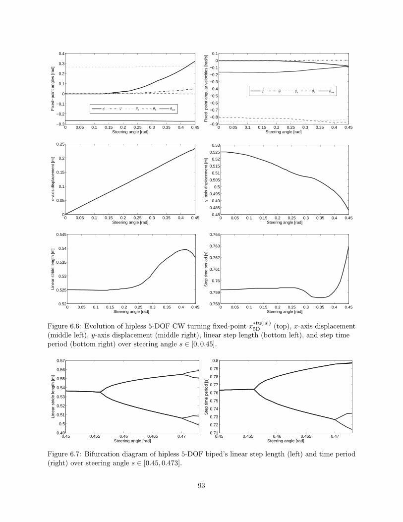
0 0.05 0.1 0.15 0.2 0.25 0.3 0.35 0.4 0.45−0.3

−0.2

−0.1

0

0.1

0.2

0.3

0.4

Steering angle [rad]

Fix

ed−

poin

t ang

les

[rad

]

ψ ϕ θs θt θns

0 0.05 0.1 0.15 0.2 0.25 0.3 0.35 0.4 0.45−0.9

−0.8

−0.7

−0.6

−0.5

−0.4

−0.3

−0.2

−0.1

0

0.1

Steering angle [rad]

Fix

ed−

poin

t ang

ular

vel

ociti

es [r

ad/s

]

ψ ϕ θs θt θns

0 0.05 0.1 0.15 0.2 0.25 0.3 0.35 0.4 0.450

0.05

0.1

0.15

0.2

0.25

Steering angle [rad]

x−ax

is d

ispl

acem

ent [

m]

0 0.05 0.1 0.15 0.2 0.25 0.3 0.35 0.4 0.450.48

0.485

0.49

0.495

0.5

0.505

0.51

0.515

0.52

0.525

0.53

Steering angle [rad]

y−ax

is d

ispl

acem

ent [

m]

0 0.05 0.1 0.15 0.2 0.25 0.3 0.35 0.4 0.450.52

0.525

0.53

0.535

0.54

0.545

Steering angle [rad]

Line

ar s

trid

e le

ngth

[m]

0 0.05 0.1 0.15 0.2 0.25 0.3 0.35 0.4 0.450.758

0.759

0.76

0.761

0.762

0.763

0.764

Steering angle [rad]

Ste

p tim

e pe

riod

[s]

Figure 6.6: Evolution of hipless 5-DOF CW turning fixed-point x∗tu(|s|)5D (top), x-axis displacement

(middle left), y-axis displacement (middle right), linear step length (bottom left), and step timeperiod (bottom right) over steering angle s ∈ [0, 0.45].

0.45 0.455 0.46 0.465 0.470.49

0.5

0.51

0.52

0.53

0.54

0.55

0.56

0.57

Steering angle [rad]

Line

ar s

trid

e le

ngth

[m]

0.45 0.455 0.46 0.465 0.470.71

0.72

0.73

0.74

0.75

0.76

0.77

0.78

0.79

0.8

Steering angle [rad]

Ste

p tim

e pe

riod

[s]

Figure 6.7: Bifurcation diagram of hipless 5-DOF biped’s linear step length (left) and time period(right) over steering angle s ∈ [0.45, 0.473].

93

−0.3 −0.2 −0.1 0 0.1 0.2 0.3 0.4 0.5−2.5

−2

−1.5

−1

−0.5

0

0.5

1

1.5

2

2.5

Angular position [rad]

Ang

ular

vel

ocity

[rad

/sec

]

(ψ, ψ) (ϕ, ϕ) (θs, θs) (θns, θns)

0 0.1 0.2 0.3 0.4 0.5 0.6 0.7 0.8−0.3

−0.2

−0.1

0

0.1

0.2

0.3

0.4

0.5

Time [sec]

Ang

ular

pos

ition

[rad

]

ψ ϕ θs θns

00.5

11.5

2

−0.5

0

0.5

1

0

0.2

0.4

0.6

0.8

Figure 6.8: Hipless 4-DOF CW s-turning 1-step gait: phase portrait (top), coordinate trajectories(middle), and 13-step 360-turn animation (bottom).

94

Similarly, we demonstrate turning gaits for the 5-DOF biped by choosing s = 0.32:

x∗tu(s)5D ≈ (−0.1287,−0.019,−0.2701, 0.003, 0.2701,−0.109, 0.0172,−1.3391, 0.0659,−1.6091)T

x∗tu(−s)5D ≈ (0.1287, 0.019,−0.2701, 0.003, 0.2701, 0.109,−0.0172,−1.3391, 0.0659,−1.6091)T .

The CW-turning gait is illustrated in Fig. 6.9 (and CCW by symmetry). We see in Fig. 6.6

that the nominal walking arc for this CW gait primitive is characterized by δx∗pos = 0.1679 m and

δy∗pos = 0.5066 m.

Finally, we emphasize that these turning gaits naturally arise from our asymptotically stable

straight-ahead systems, without changing any reference trajectories. Integrating qT τ to obtain

net work per step, the specific mechanical cost of transport for each gait is cmt(x∗st4D) = 0.052,

cmt(x∗tu(±s)4D ) = 0.06, cmt(x

∗st5D) = 0.038, and cmt(x

∗tu(±s)5D ) = 0.04, which compare favorably with

the costs of other mechanisms shown in Fig. 5.13. We now must numerically derive the switching

rules discussed in Section 6.3 for these primitive sets.

6.5.3 Computing the switching rules

Although it is computationally difficult to find the exact region [−S, S], we can easily verify con-

tainment of a particular s through simulation. Therefore, we can confirm the conditions of Lemma

7 starting with 4-DOF primitive set P s4D = Gst4D,G

tu(s)4D ,Gtu(−s)

4D , i.e., s = 0.4833 ∈ [−S4D, S4D].

This corresponds to

x∗st4D, x∗tu(s)4D , x

∗tu(−s)4D ∈ BoA

(x∗st4D

) ⋂BoA

(x∗tu(s)4D

) ⋂BoA

(x∗tu(−s)4D

).

This overlapping attractive region influences the minimum dwell time N along primitives for The-

orem 13. We simulate worst-case gait switching tests to estimate N for this primitive set.

Based on the intuition provided by Theorem 13, worst-case walking scenarios are those with high

frequencies of switching gait transitions (i.e., dwell time k < N). The more often a biped switches

between gait primitives, the more likely it will accumulate transient perturbations that cannot be

attenuated during the short duration of each gait transition. Eventually, the impact-event state

from one gait primitive will be outside the basin of attraction of the next.

We first simulate switching between two fixed primitives at every step (i.e., k = 1). Both the CW-

to-CCW and CW-to-Straight cases eventually converge to 2- and 4-periodic cycles, respectively,

95

−0.3 −0.2 −0.1 0 0.1 0.2 0.3 0.4 0.5−2

−1.5

−1

−0.5

0

0.5

1

1.5

2

Angular position [rad]

Ang

ular

vel

ocity

[rad

/sec

]

(ψ, ψ) (ϕ, ϕ) (θs, θs) (θt, θt) (θns, θns)

0 0.1 0.2 0.3 0.4 0.5 0.6 0.7 0.8−0.3

−0.2

−0.1

0

0.1

0.2

0.3

0.4

0.5

Time [sec]

Ang

ular

pos

ition

[rad

]

ψ ϕ θs θt θns

0 0.5 1 1.5 2 2.5 3

−1

0

1

2

0

0.5

1

Figure 6.9: Hipless 5-DOF CW s-turning 1-step gait: phase portrait (top), coordinate trajectories(middle), and 13-step 360-turn animation (bottom).

96

0 10 20 30 40 50 60 70−5

−4

−3

−2

−1

0

1

Time [sec]

Ang

ular

pos

ition

[rad

]

ψ ϕ θs θns

Figure 6.10: Hipless 4-DOF biped’s random walk with gait dwell time k = 2 over 100 steps.

showing that the biped is robust for periodic switching transitions. This convergent behavior of

k-step steering patterns to mk-periodic gaits, for some positive integer m, demonstrates another

strength of asymptotically stable walking.

We next try a “random walk,” picking a gait primitive at every step from a uniform random

distribution. Here, we observe occasional falls, e.g., the sequence S = (s, 0, 0, 0, s, 0, 0, 0), implying

that N > 1. Setting k = 2 (switching allowed every other step), we are unable to produce falls

after several lengthy simulations (400+ steps, e.g., Fig. 6.10), suggesting that minimum dwell

time N = 2. This is evidence that the overlapping attractive region of our primitive set is large,

presumably due to the close proximity of the set’s fixed-points, e.g., d(x∗tu(s)4D , x

∗tu(−s)4D ) < 0.064, as

well as the large size of each gait’s basin of attraction. Hence, the 4-DOF primitive set is capable

of building a large class of robust walking paths through 3-D space.

The same process is performed for the 5-DOF primitive set P s5D = Gst5D,G

tu(s)5D ,Gtu(−s)

5D , confirm-

ing that s = 0.32 ∈ [−S5D, S5D] and that N = 2. We now present planned walking results using a

tree search algorithm to provide open-loop supervisory control of each model’s switched system.

6.6 Planned Walking Results

These gait primitives and their associated switching rules enable path planning (e.g., Fig. 6.11) by

exploring the action space of primitive arcs. The set of feasible action sequences, characterizing

robust paths not in collision with the environment, forms a discrete tree of walking arcs with

branching factor b = 3, the cardinality of the primitive set. This tree expands exponentially with

97

xFigure 6.11: Example of a planned path using gait primitives for hipless 5-DOF biped. Thesequence of primitives is (S, CCW, CCW, S, S, S, S, CW, CW, S, S, S, S), where switchingtransitions are signified by circles at the impact events.

O(bd), where d is the tree depth in number of steps. We must use a heuristic to prune less promising

branches (i.e., a biased sampling of the action space) in order to find paths of high depth in the

tree, which will almost always be the case when navigating a complex environment. However, any

tree search heuristic can be chosen for this planning framework, and many suitable methods exist

(e.g., the A* algorithm [110,111], applied to humanoid planning in [112]).

To simplify our planning problem, we define a goal region Rf ⊂ SE(2) so that any robust walking

path execution Ecwc0 (xe0) ending at world configuration cw ∈ Rf is considered admissible. In most

cases, this greatly enlarges the class CRfc0 of robust walking paths between c0 and Rf , allowing us to

ignore issues of reachability. We now adopt the tree search algorithm developed in [98] specifically

for this application, which performs a cell decomposition of the environment to bias tree growth

toward the desired goal region Rf . This planner outputs a sequence S(Ecwc0 (xe

0))∈ s, 0,−sw of

steering angles parameterizing the gait primitive at each step in the walking execution Ecwc0 (xe0).

The search algorithm plans candidate paths through the example obstacle environment of Fig.

6.12 using 4-DOF primitive set P s4D, parameterized by s = 0.4833, and 5-DOF primitive set P s5D,

parameterized by s = 0.32. In each case, we choose the candidate path that best approximates the

optimal path with respect to a cost function that equally penalizes the number of steps and the

number of switching transitions:

JS(Ecwc0 (xe

0))

=

w +∑w−1

i=1 1Gi 6= Gi+1 , cw ∈ Rf

∞ , cw /∈ Rf

(6.2)

98

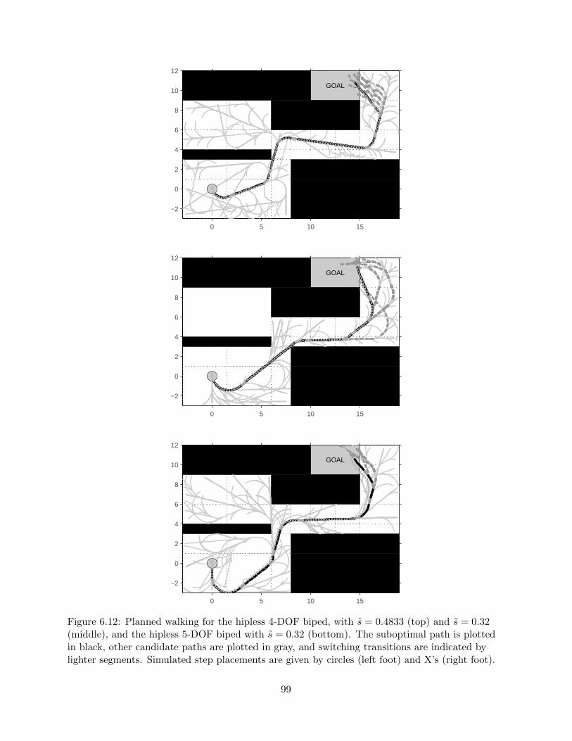
0 5 10 15

−2

0

2

4

6

8

10

12

GOAL

0 5 10 15

−2

0

2

4

6

8

10

12

GOAL

0 5 10 15

−2

0

2

4

6

8

10

12

GOAL

Figure 6.12: Planned walking for the hipless 4-DOF biped, with s = 0.4833 (top) and s = 0.32(middle), and the hipless 5-DOF biped with s = 0.32 (bottom). The suboptimal path is plottedin black, other candidate paths are plotted in gray, and switching transitions are indicated bylighter segments. Simulated step placements are given by circles (left foot) and X’s (right foot).

99

where w is the number of steps in the path execution and 1 is an indicator function that determines

whether a switching transition occurs at step i. By minimizing cost function J , the planner will

output a shorter and smoother (consequently more stable) walking path.

The example cases of Fig. 6.12 show the planned walking path (in black) and simulated walking

execution (in gray circles and X’s). Since the 4-DOF biped is more maneuverable, we also simulate

a planned execution of this model using the lower-curvature primitive set P s4D for the purpose of

comparison (note that s ∈ [−S4D, S4D] since s < s). We see that the 4-DOF biped using both

primitive sets traces the pre-planned path without any noticeable drift, whereas the 5-DOF biped

using its low-curvature set (parameterized by s) has minor drift near the end of the path execution.

Recall that the bipeds do not explicitly track these planned paths, but rather the gait primitives

accurately predict the walking path execution using the nominal walking arcs. This is noteworthy

given the transient effects after each switching transition. The minor drift observed may indeed

accumulate over longer paths, but occasional re-planning, taking a couple seconds or less, can easily

compensate for this. In more practical applications, such an iterative planner would already be

necessary to incorporate information obtained while navigating through new environments.

6.7 Remarks

The planning framework of dynamic gait primitives can be used with any control method that

produces asymptotically stable gaits (e.g., walking [35, 43, 50, 51, 79], climbing [113], or running

[6, 114]). Gait primitives and their switching rules might also be pre-computed using the feedback

motion planning method of randomized LQR trees [115].

Each gait primitive is characterized by its hybrid system dynamics and stable fixed-point, thus

corresponding to a nominal hybrid periodic orbit. In our compass-gait examples, these orbits are

naturally attractive by the (pseudo-passive) robot dynamics after controlled reduction. This motion

is not prescribed by full-state trajectories [105] or subjected to any postural constraints to ensure

stability [17,20,21], yet we have robustness over a large class of paths composed of gait primitives.

This allows decomposed tree search planning for fast and efficient bipedal locomotion based on

human-like passive walking principles, which is fundamentally different from ZMP methods. In

other words, the walking paths can be planned much like trivial Dubins curves [99]. Although

ZMP biped planners often use Dubins curves as a local planning heuristic [17], our results may

reaffirm this choice from the perspective of stability.

100

If this control/planning framework were to be applied to a practical real-world environment, we

could integrate a suite of other feedback motion planning tools, such as step-level planning over

rough terrain [41, 42] and time-scaling for variable walking speeds [38]. Experimental results have

been achieved for planar limit cycle walking (cf. [6,28]), and 3-D results may soon be possible with

advances in actuator and biped mechanical design. For example, the preliminary investigation of

[79] aims to implement controlled reduction on the highly-redundant Sarcos humanoid robot [116].

101

CHAPTER 7

EXTENSIONS TO LOCOMOTOR REHABILITATION

The field of therapeutic robotics has shown great promise in treating neuromotor disorders and

alleviating the intensive labor required by physical therapists. However, significant challenges still

remain with the design of control strategies for robot-assisted locomotor rehabilitation. In this

section, we propose extensions of our energy-shaping feedback control paradigm to address some

of these challenges. We speculate on the utility of these robot-assist strategies based on evidence

from the literature that would suggest similarities between our robot walking results and human

biomechanics.

7.1 Connections to Human Biomechanics

We first review the biomechanics literature to establish several connections to the autonomous

robot walking material presented in the previous chapters.

7.1.1 Modeling assumptions

To begin, we must consider the effect of our modeling assumptions in comparing our results to

human walking. A human gait has a substantial double-support phase including a pushoff period

(positive CoM work) followed by collision/weight-acceptance (negative CoM work) [97]. However,

the compass-gait biped has instantaneous double-support due to perfectly plastic impact events

(negative work) and immediate replenishment of potential energy (positive work) if walking on a

decline slope. For this reason, the vertical GRF plot of Fig. 5.5 lacks the extra “hump” observed

in human walking during double support [117].

The compass-gait model is therefore most useful for characterizing the midstance behavior of

human walking, which begins with “rebounding” during the upward pendular arc (positive CoM

work) and ends with “preloading” during the downward pendular arc (negative CoM work) [97].

102

Nontrivial double-support phases for the compass-gait walker have recently been considered in [26],

which might prove helpful in future analysis. Moreover, non-trivial feet are considered in the con-

trolled reduction work of [89], showing that these results can be extended to more anthropomorphic

models.

7.1.2 Turning strategies

The turning gaits of Chapters 5 and 6 exhibit the fundamental sagittal-plane periodicity of straight-

ahead gaits with slight step length and velocity adjustments. This behavior resembles the constant-

curvature human turning experiments of [94,95], in which healthy subjects walked 4 m (i.e., 6 steps)

along a constant-curvature path with radius of curvature 1.2 m. The resulting body trajectories

were segmented by three complete two-step gait cycles, each consisting of a straight-ahead trajec-

tory with steering every other step (which we reproduced in Chapter 5). Electromyography (EMG)

analysis showed that the legs propagated the same rhythm (and similar muscle activity) despite

differences in stride length and velocity between the inner and outer legs [95]. This led the authors

to suggest that human turning exploits the same “basic mechanisms of the spinal locomotor gen-

erator” as straight-ahead walking, i.e., turning gaits are built from one periodic rhythm/motion as

in our control theoretic results. We certainly do not believe that humans use a sophisticated geo-

metric approach like controlled reduction, but this observation could be explained by a locomotor

control strategy that employs some form of sagittal-plane decoupling, where the out-of-plane (i.e.,

transverse and frontal) modes synchronize to the basic sagittal-plane rhythm (with modulation for

turning).

More specifically, three distinct strategies for sharp turns have been observed in healthy human

subjects [100]. Instructed to perform a 90 turn over two steps, subjects induced steering motion

about the stance leg (“spin” turns) or stepped into the turn by appropriately placing the swing

leg (“step” turns). The former category is further decomposed into an “ipsilateral pivot,” where

the ipsilateral (i.e., stance) foot pivots into the new heading at approximately midstance, or an

“ipsilateral crossover,” where the hip swings the contralateral (i.e., swing) leg around the ipsilateral

limb into the new direction of travel. The majority of subjects employed the step turn, but our

simple 3-D models do not have the hip abduction/adduction DOFs necessary to implement this

strategy (see [35] for models that are capable of this motion).

Instead, the bipeds in Chapter 5 employ spin turns, which cannot be further distinguished due

103

to the point-foot assumption (i.e., there is no difference between rotation at the stance ankle or

foot). We were unable to successfully simulate two-step 90 turns due to the destabilizing effect of

the increased range of motion (RoM) in the transverse plane. However, [100] found that the RoM

outside the sagittal plane was smaller for step turns, suggesting that this strategy might be more

robust to sharp maneuvers than our spin turns.

7.1.3 Gait primitives and switching

Although we constructed the gait primitive framework of Chapter 6 for robot motion planning,

evidence exists for human gait primitives in the biomechanics literature. Recall that the curved

walking paths from the human trials of [94] are distinctly segmented by two-step arcs, suggesting

the composition of period-2 gait primitives. This is further supported by the study [118], in which

healthy subjects were instructed to alter their walking direction when visually cued at random.

The investigators offer three important observations from these experiments [118]:

1. Subjects were unable to alter the direction in the ongoing step, with the major constraint being the

inability to rotate the body in the appropriate direction within a step duration.

2. The majority of the subjects were unable to alter their direction of locomotion when the cue was given

one step duration ahead.

3. The success rate for a change in direction was very high (70%) when the cue was given two step

durations ahead.

This behavior could indeed be explained by planned switching between two-step gait primitives to

achieve the heading change after the unanticipated cue.

We also find evidence for locomotor primitives in studies unrelated to turning. In the plantar

flexor stretch reflex experiments of [119], an EMG-controlled powered ankle exoskeleton was used

to amplify the ankle torque of one leg during treadmill walking. Subjects completed 30 minute

training sessions with this asymmetric assistance, after which the assistance was unexpectedly

decreased during steady-state walking. Although subjects initially took several minutes to reach

steady-state with the exoskeleton assistance, they adapted to the decreased assistance by increasing

soleus muscle activity with a delay of about 60 ms. Similarly, subjects were able to quickly adapt

to reactivated assistance after the initial learning phase.

This suggests that humans with robotic assistance can learn multiple gaits involving different neu-

romotor patterns, and effectively switch among the set of acquired gaits (i.e., the gait primitives).

104

V (x0)

G1

Gk

G2 V (x∗1)

V (x∗2)

V (x∗k)

Figure 7.1: Sequential composition of Lyapunov funnels, corresponding to intermediate traininggaits, toward some nominal (healthy) gait with fixed-point x∗k. The funneled state trajectory(dotted green) corresponds to the trajectory of the funneled Lyapunov functions (solid blue).Original figure from [52] reproduced with permission of the publisher.

This may motivate progressive gait therapies based on sequential composition of intermediate

training gaits (Fig. 7.1), which can be designed a priori as in Chapter 6.

7.2 Challenges in Robot-Assisted Therapy

Recent studies with the Lokomat lower-extremity exoskeleton suggest that strategies imposing

reference gait patterns (i.e., joint position trajectories) are less effective than manual therapy in

terms of recovered walking speed and endurance for chronic stroke patients [120, 121]. Based on

similar control principles, this quasi-static form of locomotor training may indeed suffer from the

same fundamental flaws as quasi-static robot walking.

Other challenges exist in the control design for robotic ankle-foot orthosis (AFO), where control

patterns are typically tuned in an ad hoc manner based on how a healthy walking gait should look.

This requires active estimation of the intended modality (e.g., walking or standing) as well as the

phase of a gait cycle, which are prone to errors that risk life-threatening falls. Costly attention

must also be given to adapting these control sequences to individual morphology and impairment.

The impetus to address these control challenges is eloquently stated in [122]:

Robotics has the opportunity to make a quantum leap by systematically implementing and con-

trolling therapies, and by enabling systematic adjustment of treatment parameters.

105

Future work must consider novel feedback control paradigms for locomotor therapy, where control

theories from robot locomotion are translated into strategies for functional human assistance.

Recall that the potential energy provided by gravity at every step is fundamental to efficient dy-

namic locomotion, particularly passive downhill walking. These stable gaits do not track reference

patterns, but naturally appear from the system nonlinearities. The metabolic energetic cost of

human walking is minimized on shallow downhill slopes [123] by similarly exploiting the potential

energy provided by gravity. This suggests that passive walking models may relate fundamental

principles behind human dynamics to guide our design and analysis of robot-assisted therapies.

It is also known that speed-intensive training, which effectively encourages dynamic walking, im-

proves gait efficiency and muscle activation for hemiparetic1 patients [124]. This demonstrates the

importance of compliance to passive dynamics in locomotor therapy, so control strategies should

be designed to enable and encourage this motion.

7.3 Control Design Methodology

We can now use these control theoretic principles to develop assistive strategies for personalized

therapeutic benefit. The theory of Lagrangian mechanics allows direct examination of functional

characteristics of mechanical system dynamics and therefore will be useful in control design.

The configuration of an n-DOF human-machine system is given by the vector q of generalized

coordinates in configuration space Q. Given Lagrangian function L, we consider the dynamical

equations E L qL = τ of (2.2), where n-dimensional torque vector τ = Bu+v is composed of robot

control input u and unknown human input v. Since the assistive robot input is m-dimensional with

m < n, we define n ×m-matrix B as the map from control u to the n-dimensional joint torques.

Therefore, the 2nd-order system of ordinary differential equations (2.2) has the dynamical structure

M(q)q + C(q, q)q +N(q) = Bu+ v, (7.1)

where C is the n× n Coriolis/centrifugal matrix and N = ∇qV is the potential torque vector.

Recalling that gravitational potential energy is fundamental to dynamic walking, we can use

robot input u to shape the human’s potential energy, i.e., replace known V with some V that has

beneficial properties. Since this control is underactuated (m < n), matrix B is not invertible, so

1Weakness in one side of the body, often caused by stroke.

106

only a particular set of energies are achievable from the range space of B. This has been well studied

in the literature (e.g., [58]) in terms of energy matching conditions. Given continuous dynamics

(7.1) and desired potential vector N = ∇qV, we want to enforce the equality

v = M(q)q + C(q, q)q +N(q)−Bu (7.2)

= M(q)q + C(q, q)q + N(q),

which is equivalent to the necessary condition

Bu = N(q)− N(q). (7.3)

We must characterize the null space of B, so we define the full rank left-annihilator B⊥ such that

B⊥B = 0. The right-hand side of (7.3) is in the range space of B if

B⊥N(q)− N(q) = 0, ∀ q ∈ Q. (7.4)

We can then derive the underactuated control law that exactly achieves desired potential V :

u = (BTB)−1BT N(q)− N(q). (7.5)

In order to develop a strategy for personalized locomotor therapy, we propose three guiding

principles for selecting virtual potential energy V for the patient:

1. Satisfy energy matching condition (7.4).

2. Preserve the natural limit cycle known to exist in the human dynamics.

3. Alter specific dynamical characteristics based on impairment.

Preliminary work in [125] designs such a strategy for the portable-powered AFO of [126], using

one actuated DOF to reduce the perceived weight of a patient’s center of mass. In other words,

virtual V can be chosen as the original potential energy with a smaller hip mass to mimic the

body-weight support/stability provided by conventional harnesses. Computer simulations of passive

walkers demonstrate that increased body-weight support reduces stride length, velocity, and human

work, while improving energy regulation and stability. This suggests that slow walking can be

enabled at the onset of therapy for stroke-induced paresis, in order to encourage progressively

107

faster, more natural gaits as the assistance is gradually decreased. Moreover, the simple feedback

control architecture is independent of gait modality and defined in terms of physical parameters

that can be easily tuned to individual need.

7.4 Potential Impact

The need for accessible and personalized locomotor therapy after stroke continues to grow with

the aging population in the United States. In order for assistive robotics to meet this demand, a

systematic approach for functional control design must be developed to address current challenges

in automated therapy. This will yield control strategies that modify meaningful characteristics

of impaired gaits through feedback loops without reference patterns. Passive walking simulations

may then allow “rapid prototyping” of personalized strategies by predicting effects on specific

impairments, helping clinicians prescribe sequential locomotor therapies based on intermediate

training gaits (designed a priori).

The therapeutic value of control theories such as kinetic-energy shaping and passivity-based con-

trol could also be studied, in order to determine the most effective control paradigms for locomotor

training. This will enable therapies to be widely automated with active AFO or lower-extremity

exoskeletons such as Lokomat. Moreover, this could be applied to portable-powered AFO devices

(e.g., [126]) for long-term use at home. This will assist elders with decreased mobility and in-

creased risk for life-threatening falls (especially after stroke). This also offers a simple alternative

to exoskeletal performance augmentation (cf. [127]) for carrying heavy equipment near the body’s

center of mass, where the virtual mass can be tuned to the human’s mass without payload.

Likewise, potential-energy shaping has promise for assisted control of neuroprosthetic lower limbs.

Control theoretic strategies could serve as autonomous components to lower-extremity neural con-

trol systems, counteracting the destabilizing effect of gravity at high speeds to enable natural

walking without canes or crutches. This is particularly relevant in the United States, where lower-

extremity amputation rates are higher than other developed countries.

108

CHAPTER 8

CONCLUSIONS

This thesis has shown that reduction-based control enables fully 3-D bipedal robots to walk dy-

namically based on human-like passivity principles. The energy-shaping control paradigm, and

controlled reduction in particular, aim by construction to minimally cancel system nonlinearities

and thus achieve energetic efficiency with natural swaying motion. In fact, we saw that reduction-

based control is fundamentally related to passive feedback and thus inverse-optimality.

Our results require only the existence of stable limit cycles in the sagittal subsystem, thus

simplifying the search for full-order stable limit cycles and expanding the class of walking robots

that can stably exploit passive dynamics to a subset of 3-D open kinematic chains. We have a

reasonable understanding of limit cycle stability, since the high-dimensional basin of attraction

depends primarily on the sagittal-plane subsystem, for which locally stable behavior is guaranteed

from anywhere on the conserved quantity surface. And because we do not enforce a particular

trajectory, overall walking gaits need not be known a priori, suggesting a natural robustness to

perturbations such as steering motions.

The sequential composition framework of dynamic gait primitives can be used with any control

method that produces asymptotically stable gaits (e.g., walking [35, 43, 50, 51, 79], climbing [113],

or running [6, 114]). This framework reduces dynamically stable motion planning for fast and

efficient dynamic locomotion to a simple tree search, enabling motion planning applications similar

to what is readily possible for inefficient quasi-static walkers. Using the developing theory of

[103, 104], the basin of attraction of each gait’s hybrid limit cycle can be conservatively estimated

to derive switching rules. Future work such as [98] will detail high-level planning algorithms that

can integrate a suite of other motion control tools, such as step-level planning over rough terrain

[41,42,128] and time-scaling for variable walking speeds [38,39]. Gait primitives and their switching

rules might also be pre-computed using the feedback motion planning method of randomized LQR

trees [115].

109

These results motivate two main thrusts of future work, one attempting to achieve dynamic

walking on practical humanoid robots, and the other investigating the value of energy-shaping

control in robot-assisted locomotor rehabilitation.

8.1 Autonomous Robot Walking

Experimental results have been achieved for planar limit cycle walking (cf. [6,28]), and 3-D results

may soon be possible with advances in actuator and biped design. As discussed in Section 5.6,

this will likely require the degree-one underactuated implementation of our reduction-based control

method, where the ankles have passive damping in the yaw DOF and torque control in lean and

pitch (like that of a human). High power-density ankle actuators (i.e., small size with high power

output) are becoming more common, but comparable spherical actuators for roll, pitch, and yaw

remain a significant challenge in mechanical design.

We presented the general k-stage case of reduction-based control for n-DOF open kinematic

chains, so this method extends to higher-dimensional robotic systems. This could potentially be

applied to highly-redundant humanoids with articulated arms that can interact with the environ-

ment. However, we have seen that energy-shaping control laws require n×n matrix inverses, often

making these control theories difficult to scale to high-dimensional systems (in terms of computation

time and modeling error amplified by inversion).

The recent work [79] presents a first step towards the application of energy-shaping methods

on real humanoid robots by casting controlled reduction into a framework of acceleration-based

inverse dynamics. Representing the momentum conservation laws as constraints in acceleration

space, a general expression can be constructed for desired joint accelerations that render the con-

straint surface invariant. The unconstrained (reduced) dynamics can then be decoupled from the

constrained dynamics by appropriately choosing an orthogonal projection. This planar subsystem

(a double-integrator) can be stabilized by any acceleration-based controller, including passivity-

based/energy-shaping methods. The overall control law is surprisingly simple, requiring only a

k × k matrix inverse, and represents a practical way for robotic platforms to employ control theo-

retic stability results. This line of work has reproduced the 5-DOF bipedal walking results of Section

5.4 to show correspondence between the new and original controllers, and preliminary balancing

results for a 16-DOF lower-extremity Sarcos humanoid [116] demonstrate the future applicability

of this method.

110

After addressing such implementation challenges, gait primitive theory could allow complex

robots with active control to embrace passive dynamics for dynamic walking between desired lo-

cations. Such robots could perform tasks while having great autonomy from base stations, as the

efficient and natural walking gaits would allow significant locomotion range and long battery life

(arguably superior to related characteristics of quadrupedal and treaded robots [13]). These are

absolute necessities if robotic technologies are to be implemented on intelligent prosthetic legs or

assisted walking devices for the elderly or disabled. There are similar applications in the manufac-

turing industry, where versatile and long-lasting robots are desirable for the varying demands of

lean manufacturing environments. This raises interesting questions about biped coordination, such

as synchronizing robot marching given differing initial conditions and asynchronous parameters.

8.2 Robot-Assisted Locomotor Rehabilitation

Evidence from the biomechanics literature in Chapter 7 suggests that feedback control paradigms

such as energy shaping may have value as novel strategies for robot-assisted locomotor rehabilita-

tion. This future work aims to establish systematic design methods for personalized control strate-

gies that provably modify meaningful characteristics of the human gait. This must also address

challenges related to the underactuated nature of the robot control authority in the human-machine

system, where the human control policy is unknown.

Preliminary applications of these ideas include portable-powered ankle-foot orthosis (AFO) with

one actuated DOF such as [126]. The paper [125] proposes a control theoretic strategy for this

device based on the methodology discussed in Section 7.3, underactuated potential energy shaping.

This yields a simple control law that lessens the perceived weight of the patient’s center of mass,

and simulations indicate this will provide energy regulation and improved stability through pro-

gressive training regiments designed with Lyapunov funneling in mind. Given current challenges

in developing effective robotic locomotor therapies for stroke patients [120–122], this line of work

can potentially offer novel systematic approaches to control strategy design.

The discussion of Section 7.1.3 also begs deeper questions about the building blocks of human

locomotion: is our motion based on a set of gait primitives in the form of neuromuscular memory

and periodic rhythms from the spinal cord’s central pattern-generator? The relevance of these

questions and our motivating results will continue to grow as the medical, industrial, and military

sectors become increasingly interested in legged robotics.

111

APPENDIX A

PROPERTIES OF ALMOST-CYCLIC LAGRANGIAN

SYSTEMS

Since reduction-based control shapes the kinetic and potential characteristics of robots, we must

consider whether the well-known properties of general robotic systems still hold. To begin, almost-

cyclic systems do not preserve the linearity-in-the-parameters property, which provides that the

E-L equations can be “linearly” expressed by

d

dt∇qL −∇qL = Y (q, q, q)Θ,

where Θ ∈ Rp is the parameter vector of constants, in terms of link masses, inertias, and lengths,

and Y ∈ Rn×p is the regressor matrix of nonlinear functions of (q, q, q), as discussed in [55]. This

property does not hold because reduction-based control laws require matrix inversion (demonstrated

in Section 4.3), introducing rational dependencies on q in the system dynamics and thus breaking

linearity in the parameters. This can explicitly be seen in the almost-cyclic matrix Mλk1of (4.4).

On the other hand, several important properties of robotic systems do hold for k-ACL systems.

After shaping a standard robot’s Lagrangian to a k-ACL through reduction-based control law (4.8),

we prove the following properties are preserved:

1. Symmetry of the inertia matrix

2. Positive definiteness of the inertia matrix

3. Skew-symmetry of the inertia matrix minus twice the Coriolis matrix

These properties are used in Theorem 7 to show that passivity is also preserved.

A.1 Inertia Matrix

Theorem 14. Given a k-almost-cyclic Lagrangian, its inertia matrix Mλk1(qn2 ) is symmetric and

positive definite.

112

Proof. Recall that k-almost-cyclic inertia matrix Mλk1(qn2 ) is defined in (4.4) by

Mλk1(qn2 ) = M(qn2 ) +

k∑i=1

0 0

0MTqi,q

ni+1

(qni+1)Mqi,qni+1

(qni+1)

mqi (qni+1)

.

First, we know that inertia matrix M(qn2 ) is symmetric and positive definite. Also, each summation

term 0 0

0MTqi,q

ni+1

(qni+1)Mqi,qni+1

(qni+1)

mqi (qni+1)

, i ∈ 1, k,

is symmetric since the zero terms are trivially symmetric and since mqi(qni+1) is scalar/symmetric

and (MTqi,qni+1

(qni+1)Mqi,qni+1(qni+1)

)T= MT

qi,qni+1(qni+1)Mqi,qni+1

(qni+1).

Each summation term is positive semidefinite since there are i zero-eigenvalues and since mqi(qni+1)

is positive definite by the positive definiteness of M(qn2 ) and MTqi,qni+1

(qni+1)Mqi,qni+1(qni+1) is trivially

positive definite. Finally, the sum of symmetric matrices is symmetric, and the sum of a positive

definite matrix with positive semidefinite matrices is positive definite.

A.2 Skew-Symmetry

Given a k-almost-cyclic Lagrangian, its Coriolis-gyroscopic matrix is

Cλk1(q, q) = CM

λk1

(qn2 , q) + CQλ1 (q) + . . .+ CQλk (qnk ), (A.1)

where CMλk1

(qn2 , q) ∈ Rn×n is derived from Mλk1(qn2 ) and CQλi (q

ni ) ∈ Rn×n is derived from

Qλi(qni ) =

(0 −λi(qi)m−1

qi (qni+1)Mqi,qni+1(qni+1)

)T, i ∈ 1, k.

Lemma 8. Matrix CQλi (qni ) is skew-symmetric ∀i ∈ 1, k.

Proof. This is proven by calculation for any fixed i ∈ 1, k:

CQλi (qni )q =

d

dt∇q[QTλi(q

ni )q]−∇q[QTλi(q

ni )q],

113

where

∇q[QTλi(qni )q] =

0i×1

− λi(qi)mqi (q

ni+1)M

Tqi,qni+1

(qni+1)

,

implying that

d

dt∇q[QTλi(q

ni )q] = 0i×1

− λi(qi)mqi (q

ni+1)M

Tqi,qni+1

(qni+1) + λi(qi)mqi (q

ni+1)

m2qi

(qni+1)MTqi,qni+1

(qni+1)− λi(qi)mqi (q

ni+1)M

Tqi,qni+1

(qni+1)

.

Also, the second term of CQλi (qni )q is given by

∇q[QTλi(qni )q] =

0(i−1)×1

−∂λi(qi)∂qi

1mqi (q

ni+1)Mqi,qni+1

(qni+1)qni+1

− λi(qi)mqi (q

ni+1)

∂Mqi,qni+1

(qni+1)

∂qni+1

T

qni+1 + λi(qi)m2qi

(qni+1)MTqi,qni+1

(qni+1)∂mqi (q

ni+1)

∂qni+1

Tqni+1

.

In this context, we have (note that dydt := (∂y∂t )

T and ∂(yT )∂x = ( ∂y∂x)T for all vectors x, y [129]):

λi(qi) =∂λi(qi)

∂qiqi

mqi(qni+1) = mT

qi(qni+1) =

∂mqi(qni+1)

∂qni+1

T

qni+1

MTqi,qni+1

(qni+1) =∂Mqi,qni+1

(qni+1)

∂qni+1

T

qni+1,

so after canceling terms we get

CQλi (qni )q =

0(i−1)×1

∂λi(qi)∂qi

1mqi (q

ni+1)Mqi,qni+1

(qni+1)qni+1

−∂λi(qi)∂qi

1mqi (q

ni+1)M

Tqi,qni+1

(qni+1)qi

,

implying that

CQλi (qni ) =

0(i−1)×(i−1) 0(i−1)×1 0(i−1)×(n−i)

01×(i−1) 0 ∂λi(qi)∂qi

1mqi (q

ni+1)Mqi,qni+1

(qni+1)

0(n−i)×(i−1) −∂λi(qi)∂qi

1mqi (q

ni+1)M

Tqi,qni+1

(qni+1) 0(n−i)×(n−i)

.

114

Hence, CQλi is skew-symmetric.

Theorem 15. The skew-symmetry property holds for a k-almost-cyclic Lagrangian system, i.e.,

matrix (Mλk1− 2Cλk1

) is skew-symmetric.

Proof. According to Equation (A.1),

Mλk1− 2Cλk1

= (Mλk1− 2CM

λk1

)− 2CQλ1 − . . .− 2CQλk .

Since Mλk1is symmetric by Theorem 14, and CM

λk1

is derived from Mλk1, it follows that (Mλk1

−2CM

λk1

) is skew-symmetric (see the original skew-symmetry property in [55]). Moreover, the ad-

ditional CQλi terms are skew-symmetric by Lemma 8. Finally, the summation of skew-symmetric

terms is skew-symmetric.

115

APPENDIX B

PROOF OF CONTROLLED REDUCTION THEOREM

We now revisit [49] to prove Theorem 10 from Section 4.3 (note that this proof is based on the

construction from [130]).

Proof. We begin this proof by inductively relating the vnk+1-controlled E-L equations of Lλk1 to the

k-reduced controlled E-L equations of Rλ. We will then be able to show the direct correspondence

of solutions based on the uniqueness of solutions to well-behaved differential equations.

For the general case of reduction stage-j, where j ∈ 1, k−1, we consider the generalized ACL1

Lλkj in terms of its nested ACL and remaining term:

Lλkj (qj , qnj+1, qj , q

nj+1) = Lλkj+1

(qnj+1, qnj+1) + Remj(qj , q

nj+1, qj , q

nj+1),

and similarly for the base case of stage-k, we have

Lλkk(qk, qnk+1, qk, q

nk+1) = Rλ(qnk+1, q

nk+1) + Remk(qk, q

nk+1, qk, q

nk+1),

where, for l ∈ 1, k, the remaining term is apparent from (4.7):

Reml(qnl , q

nl ) =

1

2mql(q

nl+1)(ql)

2 + qlMql,qnl+1

(qnl+1)qnl+1

+1

2qn

T

l+1

MTql,q

nl+1

(qnl+1)Mql,qnl+1

(qnl+1)

mql(qnl+1)

qnl+1

− λl(ql)

mql(qnl+1)

Mql,qnl+1

(qnl+1)qnl+1 +1

2

λl(ql)2

mql(qnl+1)

.

1This generalized almost-cyclic Lagrangian is the parent of the jth stage of reduction, as opposed to the targetRouthian of the stage-j projection.

116

Therefore, the controlled E-L equations for the general case are

d

dt

∂Lλkj∂qj

−∂Lλkj∂qj

=d

dt

∂Remj

∂qj− ∂Remj

∂qj= 0 (B.1)

d

dt

∂Lλkj∂qi

−∂Lλkj∂qi

=d

dt

∂Lλkj+1

∂qi−∂Lλkj+1

∂qi+d

dt

∂Remj

∂qi− ∂Remj

∂qi(B.2)

=

0(k−j)×1

Bqnk+1vnk+1

ei−j

for i ∈ j + 1, n, where ei−j is the (i− j)th standard basis vector for Rn−j . As for the base case,

we have

d

dt

∂Lλkk∂qk

−∂Lλkk∂qk

=d

dt

∂Remk

∂qk− ∂Remk

∂qk= 0 (B.3)

d

dt

∂Lλkk∂qi

−∂Lλkk∂qi

=d

dt

∂Rλ∂qi− ∂Rλ

∂qi+d

dt

∂Remk

∂qi− ∂Remk

∂qi= Bqnk+1

vnk+1ei−k (B.4)

for i ∈ k + 1, n, where ei−k is the (i− k)th standard basis vector for Rn−k.

It is now necessary to calculate the derivatives of Reml(qnl , q

nl ), for l ∈ 1, k:

d

dt

∂Reml

∂ql=

d

dt(Mql,q

nl+1

(qnl+1))qnl+1 +Mql,qnl+1

(qnl+1))qnl+1 +mql(qnl+1)ql (B.5)

+d

dt(mql(q

nl+1))ql

∂Reml

∂ql= −

∂∂ql

(λl(ql))

mql(qnl+1)

Mql,qnl+1

(qnl+1))qnl+1 +λl(ql)

∂∂q1

(λl(ql))

mql(qnl+1)

(B.6)

117

d

dt

∂Reml

∂qi= qn

T

l+1

Mql,qnl+1

(qnl+1)TMql,qnl+1

(qnl+1)

mql(qnl+1)

ei−1 (B.7)

+qnT

l+1

ddt(Mql,q

nl+1

(qnl+1))TMql,qnl+1

(qnl+1)

mql(qnl+1)

ei−1

+qnT

l+1

Mql,qnl+1

(qnl+1)T ddt(Mql,q

nl+1

(qnl+1))

mql(qnl+1)

ei−1

− d

dt(mql(q

nl+1))qn

T

l+1

Mql,qnl+1

(qnl+1)TMql,qnl+1

(qnl+1)

mql(qnl+1)2

ei−1

+qlMql,qnl+1

(qnl+1)ei−1 + qld

dt(Mql,q

nl+1

(qnl+1))ei−1

+λl(ql)

ddt(mql(q

nl+1))

mql(qnl+1)2

Mql,qnl+1

(qnl+1)ei−1

−ddt(λl(ql))

mql(qnl+1)

Mql,qnl+1

(qnl+1)ei−1 −λl(ql)

mql(qnl+1)

d

dt(Mql,q

nl+1

(qnl+1))ei−1

∂Reml

∂qi= 2qn

T

l+1

∂∂qi

(Mql,qnl+1

(qnl+1))TMql,qnl+1

(qnl+1)

2mql(qnl+1)

qnl+1 (B.8)

−qnTl+1

∂∂qi

(mql(qnl+1))Mql,q

nl+1

(qnl+1)TMql,qnl+1

(qnl+1)

2mql(qnl+1)2

qnl+1

+1

2

∂

∂qi(mql(q

nl+1))(ql+1)2 + ql

∂

∂qi(Mql,q

nl+1

(qnl+1))qnl+1

+

∂∂qi

(mql(qnl+1))λl(ql)

mql(qnl+1)2

Mql,qnl+1

(qnl+1)qnl+1

− λl(ql)

mql(qnl+1)

∂

∂qi(Mql,q

nl+1

(qnl+1))qnl+1 −1

2

∂∂qi

(mql(qnl+1))λl(ql)

2

mql(qnl+1)2

,

where i ∈ l + 1, n. Given these expressions, we can prove that the E-L equations for Reml hold

when restricted to the constrained surface defined by (4.2). In particular, this constraint implies

the following derivative of λl(ql) and second derivative of ql:

d

dt(λl(ql)) =

∂

∂ql(λl(ql))ql =

∂Reml

∂ql, (B.9)

ql =ddt(mql(q

nl+1))

mql(qnl+1)2

Mql,qnl+1

(qnl+1)qnl+1 −ddt(mql(q

nl+1))

mql(qnl+1)2

λl(ql) (B.10)

+ddt(λl(ql))

mql(qnl+1)

−ddt(Mql,q

nl+1

(qnl+1))

mql(qnl+1)

qnl+1 −Mql,q

nl+1

(qnl+1)

mql(qnl+1)

qnl+1.

118

Then, (B.5) and (B.6) given (4.2), (B.9), (B.10) implies

[d

dt

∂Reml

∂ql− ∂Reml

∂ql

]∣∣∣∣Jl(q

nl ,q

nl )=λl(ql)

= 0. (B.11)

And, (B.7) given (4.2) and (B.10) implies

d

dt

∂Reml

∂qi

∣∣∣∣Jl(q

nl ,q

nl )=λl(ql)

= 0.

And, (B.8) given (4.2) implies∂Reml

∂qi

∣∣∣∣Jl(q

nl ,q

nl )=λl(ql)

= 0.

Hence, we have

[d

dt

∂Reml

∂qi− ∂Reml

∂qi

]∣∣∣∣Jl(q

nl ,q

nl )=λl(ql)

= 0, (B.12)

for i = l + 1, . . . , n, showing that the E-L equations for Reml hold given that the functional

quantities are conserved.

Then, by the single-stage reduction proof of [46], based on the uniqueness of solutions to well-

behaved differential equations, we know that solutions can be related through the single-stage

reduction of both the general case and the base case. Hence, the multistage theorem follows by

induction, proving the relationship between solutions of full-order vector field fλk1and solutions of

k-reduced vector field fRλ .

119

APPENDIX C

BIPED INERTIA MATRIX TERMS

Recall that the inertia matrix of an n-DOF biped has the form

M(ϕ, θ) =

mψ(ϕ, θ) —– Mψϕθ(ϕ, θ)

| mϕ(θ) Mϕθ(θ)

MTψϕθ(ϕ, θ) MT

ϕθ(θ) Mθ(θ)

.

We now give expressions for these symbolic modeling terms corresponding to the two biped models

in Section 5.1. To obtain the analogous hipless models from Section 6.5, set hip width w = 0 and

leg splay angle ρ = 0 in the expressions below.

C.1 4-DOF Hipped Biped

In the 4-DOF model, the submatrix of M4D corresponding to the sagittal subsystem is given by

Mθ(θ) =

l2

4 (5m+ 4M) cos(ρ)2 − l2m2 cos(θs − θns) cos(ρ)2

− l2m2 cos(θs − θns) cos(ρ)2 l2m

4 cos(ρ)2

.

The lean DOF terms in the 3× 3 inertia submatrix are given by

mϕ(θ) =1

32(4l2(13m+ 6M) + 8(4m+M)w2

+l(−4l(7m+ 2M) cos(2ρ) + lm cos(2(ρ− θns)) + 2lm cos(2θns)

+lm cos(2(ρ+ θns))

+4(l cos(ρ)2(−8m cos(θns) cos(θs) + (5m+ 4M) cos(2θs))

−8(3m+M)w sin(ρ))))

Mϕθ(θ) =

− l4 cos(ρ)(−2(2m+M)w + l(7m+ 4M) sin(ρ)) sin(θs)

lm4 cos(ρ)(−2w + 3l sin(ρ)) sin(θns)

T

.

120

Finally, the yaw DOF terms in M4D are given by

mψ(ϕ, θ) =1

16(2l(4l cos(ρ)2(3m+ 2M − 2m cos(θns − θs)) sin(ϕ)2

+4w cos(ρ)(−m cos(θns) + (2m+M) cos(θs)) sin(2ϕ)

−l(−3m cos(θns) + (7m+ 4M) cos(θs)) sin(2ρ) sin(2ϕ))

− cos(ϕ)2(−2(l2(13m+ 6M) + 2(4m+M)w2)

+l2 cos(2ρ)(14m+ 4M +m cos(2θns)

+(5m+ 4M) cos(2θs) + 8m sin(θns) sin(θs))

+l(lm cos(2θns) + l(5m+ 4M) cos(2θs)

+8(2(3m+M)w sin(ρ) + lm sin(θns) sin(θs))))).

Mψϕθ(ϕ, θ) =(mψ,ϕ(ϕ, θ) mψ,θs(ϕ, θ) mψ,θns(ϕ, θ)

),

mψ,ϕ(ϕ, θ) =1

8l(4w cos(ρ) sin(ϕ)(−m sin(θns) + (2m+M) sin(θs))

−l sin(2ρ) sin(ϕ)(−3m sin(θns) + (7m+ 4M) sin(θs))

−l cos(ρ)2 cos(ϕ)(m sin(2θns) + (5m+ 4M) sin(2θs)− 4m sin(θns + θs))),

mψ,θs(ϕ, θ) =1

8l(4(2m+M)w cos(ρ) cos(ϕ) cos(θs)− l(7m+ 4M) cos(ϕ) cos(θs) sin(2ρ)

+2l cos(ρ)2(5m+ 4M − 2m cos(θns − θs)) sin(ϕ)),

mψ,θns(ϕ, θ) = −1

4lm cos(ρ)(cos(ϕ) cos(θns)(2w − 3l sin(ρ))

+l cos(ρ)(−1 + 2 cos(θns − θs)) sin(ϕ)).

C.2 5-DOF Hipped Biped

In the 5-DOF model, the submatrix of M5D corresponding to the sagittal subsystem is given by

Mθ(θ) =

14 l

2(5m+ 4(Mh +Mt)) cos(ρ)2 ltlMt cos(ρ) cos(θs − θt) − 12 l

2m cos(ρ)2 cos(θns − θs)ltlMt cos(ρ) cos(θs − θt) l2tMt 0

− 12 l

2m cos(ρ)2 cos(θns − θs) 0 14 l

2m cos(ρ)2

.

121

The lean DOF terms in the 4× 4 inertia submatrix are given by

mϕ(θ) =1

4(−4l2m cos(ρ)2 cos(θns) cos(θs) + 8ltlMt cos(ρ) cos(θs) cos(θt)

+m cos(θns)2(5l2 + 4w2 − 4l2 cos(2ρ) + 12lw sin(ρ))

+ cos(θs)2(l2(3m+ 4Mh + 2Mt) +Mhw

2

+2l2(m+Mt) cos(2ρ) + 4lMhw sin(ρ))

+Mt cos(θt)2(4l2t + w2 + 4l sin(ρ)(w + l sin(ρ)))

+m(2w + 3l sin(ρ))2 sin(θns)2 +Mhw

2 sin(θs)2

+4lMhw sin(ρ) sin(θs)2 + l2m sin(ρ)2 sin(θs)

2

+4l2Mh sin(ρ)2 sin(θs)2Mt(w + 2l sin(ρ))2 sin(θt)

2).

Mϕθ(θ) =

14 l cos(ρ)(2(2m+Mh +Mt)w + l(7m+ 4(Mh +Mt)) sin(ρ)) sin(θs)

12 ltMt(w + 2l sin(ρ)) sin(θt)

−14 lm cos(ρ)(2w + 3l sin(ρ)) sin(θns)

T

.

122

Finally, the yaw DOF terms in M5D are given by

mψ(ϕ, θ) =1

8(cos(θs)

2 cos(ϕ)2(l2(m+ 4Mh) + 2Mhw2

+l(−l(m+ 4Mh) cos(2ρ) + 8Mhw sin(ρ)))

+2m cos(θns)2(2w + 3l sin(ρ))(cos(ϕ)2(2w + 3l sin(ρ))

+2l cos(ρ) cos(θs) sin(2ϕ)) + 2(Mt cos(θt)2 cos(ϕ)2(w + 2l sin(ρ))2

+ cos(ϕ)2(m(5l2 + 4w2 − 4l2 cos(2ρ) + 12lw sin(ρ)) sin(θns)2

−4l2m cos(ρ)2 sin(θns) sin(θs) + (l2(3m+ 4Mh + 2Mt)

+Mhw2 + 2l(l(m+Mt) cos(2ρ) + 2Mhw sin(ρ))) sin(θs)

2

+8ltlMt cos(ρ) sin(θs) sin(θt) +Mt(4l2t + w2

+4l sin(ρ)(w + l sin(ρ))) sin(θt)2) + 2(2l2tMt

+l cos(ρ)(l cos(ρ)(3m+ 2(Mh +Mt)

−2m sin(θns) sin(θs)) + 4ltMt sin(θs) sin(θt))) sin(ϕ)2

+2ltMt cos(θt)(w + 2l sin(ρ)) sin(2ϕ))

−2lm cos(ρ) cos(θns)(4l cos(ρ) cos(θs) sin(ϕ)2 + (2w + 3l sin(ρ)) sin(2ϕ))

+l cos(θs)(l(4(m+Mh +Mt)− 3m cos(2θns)) sin(2ρ) sin(2ϕ)

+4 cos(ρ)(4ltMt cos(θt) sin(ϕ)2

+w(m+Mh +Mt −m cos(2θns)) sin(2ϕ)))).

123

Mψϕθ(ϕ, θ) =(mψ,ϕ(ϕ, θ) mψ,θs(ϕ, θ) mψ,θt(ϕ, θ) mψ,θns(ϕ, θ)

),

mψ,ϕ(ϕ, θ) =1

8(−l2 cos(ρ)2 cos(ϕ)(m sin(2θns) + (5m+ 4(Mh +Mt)) sin(2θs)

−4m sin(θns + θs))− 4l2tMt cos(ϕ) sin(2θt) + (7l2m sin(2ρ) sin(θs)

+4ltMt(w + 2l sin(ρ)) sin(θt)) sin(ϕ)

+2l cos(ρ)(−4ltMt cos(θt) cos(ϕ) sin(θs)− 4ltMt cos(θs) cos(ϕ) sin(θt)

+(−m(2w + 3l sin(ρ)) sin(θns) + 2((2m+Mh +Mt)w

+2l(Mh +Mt) sin(ρ)) sin(θs)) sin(ϕ))),

mψ,θs(ϕ, θ) =1

8l(7lm cos(θs) cos(ϕ) sin(2ρ)

+2l cos(ρ)2(5m+ 4(Mh +Mt)− 2m cos(θns − θs)) sin(ϕ)

+4 cos(ρ)(cos(θs) cos(ϕ)((2m+Mh +Mt)w + 2l(Mh +Mt) sin(ρ))

+2ltMt cos(θs − θt) sin(ϕ))),

mψ,θt(ϕ, θ) =1

2ltMt(cos(θt) cos(ϕ)(w + 2l sin(ρ))

+2(lt + l cos(ρ) cos(θs − θt)) sin(ϕ)),

mψ,θns(ϕ, θ) = −1

4lm cos(ρ)(cos(θns) cos(ϕ)(2w + 3l sin(ρ))

+l cos(ρ)(−1 + 2 cos(θns − θs)) sin(ϕ)).

124

REFERENCES

[1] W. R. Leonard and M. L. Robertson, “Energetic efficiency of human bipedality,” AmericanJournal of Physical Anthropology, vol. 97, pp. 335–338, 1995.

[2] M. D. Sockol, D. A. Raichlen, and H. Pontzer, “Chimpanzee locomotor energetics and theorigin of human bipedalism,” Proceedings of the National Academy of Sciences, vol. 104,no. 30, pp. 12 265–12 269, 2007.

[3] T. McGeer, “Passive dynamic walking,” International Journal of Robotics Research, vol. 9,no. 2, pp. 62–82, 1990.

[4] A. Goswami, B. Thuilot, and B. Espiau, “Compass-like biped robot part I: Stability and bi-furcation of passive gaits,” Institut National de Recherche en Informatique et en Automatique(INRIA), Grenoble, France, Tech. Rep. 2996, 1996.

[5] E. R. Westervelt, J. W. Grizzle, and D. E. Koditschek, “Hybrid zero dynamics of planarbiped walkers,” IEEE Transactions on Automatic Control, vol. 48, no. 1, pp. 42–56, 2003.

[6] E. R. Westervelt, J. W. Grizzle, C. Chevallereau, J. H. Choi, and B. Morris, Feedback Controlof Dynamic Bipedal Robot Locomotion. New York, NY: CRC Press, 2007.

[7] Wikipedia, “Sagittal plane,” 2006. [Online]. Available: http://en.wikipedia.org/wiki/Sagittal plane.

[8] H. K. Khalil, Nonlinear Systems, 3rd ed. Upper Saddle River, NJ: Prentice Hall, 2002.

[9] L. B. Freidovich, U. Mettin, A. S. Shiriaev, and M. W. Spong, “A passive 2-DOF walker:Hunting for gaits using virtual holonomic constraints,” IEEE Transactions on Robotics,vol. 25, no. 5, pp. 1202–1208, 2009.

[10] K. Kaneko, F. Kanehiro, S. Kajita, H. Hirukawa, T. Kawasaki, M. Hirata, K. Akachi, andT. Isozumi, “Humanoid robot HRP-2,” in IEEE International Conference on Robotics andAutomation, New Orleans, LA, 2004, pp. 1083–1090.

[11] Honda Worldwide, “Asimo walking technology,” 2009. [Online]. Available: http://world.honda.com/ASIMO/technology/walking.html.

[12] M. Vukobratovic and B. Borovac, “Zero-moment point - thirty years of its life,” InternationalJournal on Humanoid Robotics, vol. 1, no. 1, pp. 157–174, 2004.

[13] A. D. Kuo, “Choosing your steps carefully: Walking and running robots,” IEEE Roboticsand Automation Magazine, vol. 14, no. 2, pp. 18–29, 2007.

125

[14] D. Hobbelen and M. Wisse, “Limit cycle walking,” in Humanoid Robots: Human-Like Ma-chines, M. Hackel, Ed. Vienna, Austria: I-TECH, 2007, pp. 277–294.

[15] S. H. Collins and A. Ruina, “A bipedal walking robot with efficient and human-like gait,”in IEEE International Conference on Robotics and Automation, Barcelona, Spain, 2005, pp.1983–1988.

[16] K. Steudel, “Limb morphology, bipedal gait, and the energetics of hominid locomotion,”American Journal of Physical Anthropology, vol. 99, pp. 345–355, 1996.

[17] E. Yoshida, C. Esteves, I. Belousov, J.-P. Laumond, T. Sakaguchi, and K. Yokoi, “Planning3-D collision-free dynamic robotic motion through iterative reshaping,” IEEE Transactionson Robotics, vol. 24, no. 5, pp. 1186–1198, 2008.

[18] O. Brock and O. Khatib, “Elastic strips: A framework for motion generation in humanenvironments,” International Journal of Robotics Research, vol. 21, no. 12, pp. 1031–1052,2002.

[19] J. J. Kuffner Jr., S. Kagami, K. Nishiwaki, M. Inaba, and H. Inoue, “Dynamically-stablemotion planning for humanoid robots,” Autonomous Robots, vol. 1, no. 12, pp. 105–118,2002.

[20] J. J. Kuffner Jr., K. Nishiwaki, S. Kagami, M. Inaba, and H. Inoue, “Motion planning forhumanoid robots,” in Robotics Research. New York, NY: Springer, 2005, pp. 365–374.

[21] K. Hauser, T. Bretl, J.-C. Latombe, K. Harada, and B. Wilcox, “Motion planning for leggedrobots on varied terrain,” International Journal of Robotics Research, vol. 27, no. 11-12, pp.1325–1349, 2008.

[22] P. Michel, J. Chestnutt, S. Kagami, K. Nishiwaki, J. J. Kuffner Jr., and T. Kanade, “GPU-accelerated real-time 3D tracking for humanoid locomotion and stair climbing,” in IEEEInternational Conference on Intelligent Robots and Systems, San Diego, CA, 2007, pp. 463–469.

[23] M. W. Spong, “Passivity based control of the compass gait biped,” in IFAC World Congress,Beijing, China, 1999.

[24] M. W. Spong and F. Bullo, “Controlled symmetries and passive walking,” IEEE Transactionson Automatic Control, vol. 50, no. 7, pp. 1025–1031, 2005.

[25] B. Morris and J. W. Grizzle, “A restricted Poincare map for determining exponentially stableperiodic orbits in systems with impulse effects: Application to bipedal robots,” in IEEEConference on Decision and Control, Seville, Spain, 2005, pp. 4199–4206.

[26] M. Scheint, M. Sobotka, and M. Buss, “Virtual holonomic constraint approach for planarbipedal walking robots extended to double support,” in IEEE Conference on Decision andControl, Shanghai, China, 2009, pp. 8180–8185.

[27] C. Chevallereau, G. Abba, Y. Aoustin, F. Plestan, E. R. Westervelt, C. Canudas-de-Wit,and J. W. Grizzle, “Rabbit: A testbed for advanced control theory,” IEEE Control SystemsMagazine, vol. 23, no. 5, pp. 57–79, 2003.

126

[28] K. Sreenath, H. W. Park, I. Poulakakis, and J. W. Grizzle, “A compliant hybrid zero dynamicscontroller for stable, efficient and fast bipedal walking on MABEL,” International Journal ofRobotics Research, 2010, submitted for publication.

[29] K. Byl and R. Tedrake, “Metastable walking machines,” International Journal of RoboticsResearch, vol. 28, no. 8, pp. 1040–1064, 2009.

[30] A. D. Kuo, “Stabilization of lateral motion in passive dynamic walking,” International Jour-nal of Robotics Research, vol. 18, no. 9, pp. 917–930, 1999.

[31] S. H. Collins, M. Wisse, and A. Ruina, “A 3-D passive dynamic walking robot with two legsand knees,” International Journal of Robotics Research, vol. 20, pp. 607–615, 2001.

[32] R. Tedrake, T. W. Zhang, and H. S. Seung, “Stochastic policy gradient reinforcement learningon a simple 3D biped,” in IEEE International Conference on Intelligent Robots and Systems,vol. 3, Sendai, Japan, 2004, pp. 2849–2854.

[33] T. Fukuda, M. Doi, Y. Hasegawa, and H. Kajima, “Multi-locomotion control of biped loco-motion and brachiation robot,” in Fast Motions in Biomechanics and Robotics, ser. LectureNotes in Control and Information Sciences. Heidelberg, Allemagne, Germany: Springer,2006, pp. 121–145.

[34] C. Chevallereau, J. W. Grizzle, and C. Shih, “Asymptotically stable walking of a five-linkunderactuated 3D bipedal robot,” IEEE Transactions on Robotics, vol. 25, no. 1, pp. 37–50,2008.

[35] C. Shih, J. W. Grizzle, and C. Chevallereau, “From stable walking to steering of a 3D bipedalrobot with passive point feet,” Robotica, 2010, submitted for publication.

[36] M. W. Spong, “The passivity paradigm in bipedal locomotion,” in International Conferenceon Climbing and Walking Robots, Madrid, Spain, 2004.

[37] M. W. Spong, J. K. Holm, and D. Lee, “Passivity-based control of bipedal locomotion,” IEEERobotics and Automation Magazine, vol. 12, no. 2, pp. 30–40, 2007.

[38] J. K. Holm, D. Lee, and M. W. Spong, “Time-scaling trajectories of passive-dynamic bipedalrobots,” in IEEE International Conference on Robotics and Automation, Roma, Italy, 2007,pp. 3603–3608.

[39] Y. Hu, G. Yan, and Z. Lin, “Time-scaling control and passive walking of bipeds with under-actuation degree one,” in IEEE Conference on Decision and Control, Atlanta, GA, 2010.

[40] J. W. Grizzle, C. H. Moog, and C. Chevallereau, “Nonlinear control of mechanical systemswith an unactuated cyclic variable,” IEEE Transactions on Automatic Control, vol. 50, no. 5,pp. 559–576, 2005.

[41] S. Ramamoorthy and B. Kuipers, “Trajectory generation for dynamic bipedal walkingthrough qualitative model based manifold learning,” in IEEE International Conference onRobotics and Automation, Pasadena, CA, 2008, pp. 359–366.

[42] I. R. Manchester, U. Mettin, F. Iida, and R. Tedrake, “Stable dynamic walking over roughterrain: Theory and experiment,” in 14th International Symposium on Robotics Research,Lucerne, Switzerland, 2009.

127

[43] R. D. Gregg, T. W. Bretl, and M. W. Spong, “Asymptotically stable gait primitives forplanning dynamic bipedal locomotion in three dimensions,” in IEEE International Conferenceon Robotics and Automation, Anchorage, AK, 2010, pp. 1695–1702.

[44] A. D. Ames, R. D. Gregg, E. D. B. Wendel, and S. Sastry, “On the geometric reductionof controlled three-dimensional bipedal robotic walkers,” in Lagrangian and HamiltonianMethods for Nonlinear Control, ser. Lecture Notes in Control and Information Sciences, vol.366. Nagoya, Japan: Springer, 2007, pp. 183–196.

[45] A. D. Ames and R. D. Gregg, “Stably extending two-dimensional bipedal walking to threedimensions,” in American Control Conference, New York, NY, 2007, pp. 2848–2854.

[46] A. D. Ames, R. D. Gregg, and M. W. Spong, “A geometric approach to three-dimensionalhipped bipedal robotic walking,” in IEEE Conference on Decision and Control, New Orleans,LA, 2007, pp. 5123–5130.

[47] M. Krstic, I. Kanellakopoulos, and P. V. Kokotovic, Nonlinear and Adaptive Control Design.New York, NY: John Wiley and Sons, Inc., 1995.

[48] R. D. Gregg and M. W. Spong, “Reduction-based control with application to three-dimensional bipedal walking robots,” in American Control Conference, Seattle, WA, 2008,pp. 880–887.

[49] R. D. Gregg and M. W. Spong, “Reduction-based control of three-dimensional bipedal walk-ing robots,” International Journal of Robotics Research, vol. 26, no. 6, pp. 680–702, 2010.

[50] R. D. Gregg and M. W. Spong, “Reduction-based control of branched chains: Applicationto three-dimensional bipedal torso robots,” in IEEE Conference on Decision and Control,Shanghai, China, 2009, pp. 8166–8173.

[51] R. D. Gregg and M. W. Spong, “Bringing the compass-gait bipedal walker to three dimen-sions,” in IEEE International Conference on Intelligent Robots and Systems, St. Louis, MO,2009, pp. 4469–4474.

[52] R. Burridge, A. Rizzi, and D. Koditschek, “Sequential composition of dynamically dexterousrobot behaviors,” International Journal of Robotics Research, vol. 18, no. 6, pp. 534–555,1999.

[53] R. Ortega, A. Loria, P. J. Nicklasson, and H. Sira-Ramirez, Passivity-Based Control of Euler-Lagrange Systems: Mechanical, Electrical, and Electromechanical Applications. New York,NY: Springer-Verlag, 1998.

[54] R. Sepulchre, M. Jankovic, and P. V. Kokotovic, Constructive Nonlinear Control. New York,NY: Springer-Verlag, 1997.

[55] M. W. Spong, S. Hutchinson, and M. Vidyasagar, Robot Modeling and Control. Hoboken,NJ: John Wiley and Sons, Inc., 2006.

[56] M. W. Spong and M. Vidyasagar, “Robust linear compensator design for nonlinear roboticcontrol,” IEEE Journal of Robotics and Automation, vol. 3, no. 4, pp. 345–351, 1987.

[57] R. Ortega and M. W. Spong, “Adaptive motion control of rigid robots: A tutorial,” in IEEEConference on Decision and Control, San Antonio, TX, 1988, pp. 1575–1584.

128

[58] R. Ortega, M. W. Spong, F. Gomez-Estern, and G. Blankenstein, “Stabilization of a classof underactuated mechanical systems via interconnection and damping assignment,” IEEETransactions on Automatic Control, vol. 47, no. 8, pp. 1218–1233, 2002.

[59] G. Blankenstein, R. Ortega, and A. J. Van Der Schaft, “The matching conditions of controlledLagrangians and IDA-passivity based control,” International Journal of Control, vol. 75,no. 9, pp. 645–665, 2002.

[60] N. Chopra and M. W. Spong, “Passivity-based control of multi-agent systems,” in Advancesin Robot Control. New York, NY: Springer-Verlag, 2007, pp. 107–134.

[61] P. Moylan, “Implications of passivity in a class of nonlinear systems,” IEEE Transactions onAutomatic Control, vol. 19, no. 4, pp. 373–381, 1974.

[62] J. E. Marsden and T. S. Ratiu, Introduction to Mechanics and Symmetry, 2nd ed. NewYork, NY: Springer, 2002.

[63] H. Cendra, J. E. Marsden, and T. S. Ratiu, Lagrangian Reduction by Stages, ser. Memoirs ofthe AMS. Providence, RI: AMS Bookstore, 2001.

[64] J. E. Marsden, J.-P. Ortega, T. S. Ratiu, G. Misiolek, and M. Perlmutter, HamiltonianReduction by Stages, ser. Lecture Notes in Mathematics. New York, NY: Springer, 2007.

[65] E. Gu, “Configuration manifolds and their applications to robot dynamic modeling and con-trol,” IEEE Transactions on Robotics and Automation, vol. 16, no. 5, pp. 517–527, 2000.

[66] M. Fliess, J. Levine, P. Martin, and P. Rouchon, “Flatness and defect of non-linear systems:Introductory theory and examples,” International Journal of Control, vol. 61, no. 6, pp.1327–1361, 1995.

[67] M. Rathinam, “Differentially flat nonlinear control systems,” Ph.D. dissertation, CaliforniaInstitute of Technology, Pasadena, CA, 1997.

[68] F. Lamiraux and J.-P. Laumond, “Flatness and small-time controllability of multibody mobilerobots: Application to motion planning,” IEEE Transactions on Automatic Control, vol. 45,no. 10, pp. 1878–1880, 2000.

[69] R. M. Murray, Z. Li, and S. S. Sastry, A Mathematical Introduction to Robotic Manipulation.Boca Raton, FL: CRC Press, 1994.

[70] P. J. Olver, Applications of Lie Groups to Differential Equations. New York, NY: Springer-Verlag, 2000.

[71] B. O’Neill, Elementary Differential Geometry, 2nd ed. San Diego, CA: Elsevier AcademicPress, 2006.

[72] P. G. Mehta, G. Hagen, and A. Banaszuk, “Symmetry and symmetry-breaking for a waveequation with feedback,” SIAM Journal of Applied Dynamical Systems, vol. 6, no. 3, pp.549–575, 2007.

[73] N. E. Leonard, “Stabilization of underwater vehicle dynamics with symmetry-breaking po-tentials,” Systems and Control Letters, vol. 32, pp. 35–42, 1997.

129

[74] E. A. Shammas, H. Choset, and A. A. Rizzi, “Geometric motion planning analysis for twoclasses of underactuated mechanical systems,” International Journal of Robotics Research,vol. 26, no. 10, pp. 1043–1073, 2007.

[75] E. A. Shammas, H. Choset, and A. A. Rizzi, “Towards a unified approach to motion planningfor dynamic underactuated mechanical systems with non-holonomic constraints,” Interna-tional Journal of Robotics Research, vol. 26, no. 10, pp. 1075–1124, 2007.

[76] A. M. Bloch, N. E. Leonard, and J. E. Marsden, “Controlled Lagrangians and the stabilizationof mechanical systems. I: The first matching theorem,” IEEE Transactions on AutomaticControl, vol. 45, no. 12, pp. 2253–2270, 2000.

[77] D. E. Chang and J. E. Marsden, “Reduction of controlled Lagrangian and Hamiltoniansystems with symmetry,” SIAM Journal on Control and Optimization, vol. 43, no. 1, pp.277–300, 2005.

[78] A. M. Bloch, D. E. Chang, N. E. Leonard, and J. E. Marsden, “Controlled Lagrangiansand the stabilization of mechanical systems. II: Potential shaping,” IEEE Transactions onAutomatic Control, vol. 46, no. 10, pp. 1556–1571, 2001.

[79] R. D. Gregg, L. Righetti, J. Buchli, and S. Schaal, “Constrained accelerations for controlledgeometric reduction: Sagittal-plane decoupling in bipedal locomotion,” in IEEE InternationalConference on Humanoid Robots, Nashville, TN, 2010.

[80] M. W. Spong, “The swing up control problem for the Acrobot,” IEEE Control SystemsMagazine, vol. 15, no. 1, pp. 49–55, 1995.

[81] M. D. Berkemeier and R. S. Fearing, “Tracking fast inverted trajectories of the underactuatedacrobot,” IEEE Transactions on Robotics and Automation, vol. 15, no. 4, pp. 740–750, 1999.

[82] G. Marmo, E. Saletan, A. Simoni, and B. Vitale, Dynamical Systems: A Differential Ge-ometric Approach to Symmetry and Reduction. New York, NY: John Wiley & Sons Inc,1985.

[83] V. A. Yakubovich and V. M. Starzhinskii, Linear Differential Equations with Periodic Coef-ficients. New York, NY: Wiley, 1975.

[84] S. P. Boyd and L. Vandenberghe, Convex Optimization. New York, NY: Cambridge Univer-sity Press, 2004.

[85] M. W. Spong and F. Bullo, “Controlled symmetries and passive walking,” in IFAC WorldCongress, Barcelona, Spain, 2002.

[86] J. Wittenburg, Dynamics of Multibody Systems, 2nd ed. New York, NY: Springer, 2007.

[87] D. Agahi and K. Kreutz-Delgado, “A star-topology dynamic model for multipedal loco-motion,” in IEEE Conference on Decision and Control, vol. 5, San Diego, CA, 1997, pp.4868–4873.

[88] S. S. Sastry, Nonlinear Systems: Analysis, Stability and Control. New York, NY: Springer-Verlag, 1999.

130

[89] R. Sinnet and A. D. Ames, “3D bipedal walking with knees and feet: A hybrid geometricapproach,” in IEEE Conference on Decision and Control, Shanghai, China, 2009, pp. 3208–3213.

[90] J. W. Grizzle, G. Abba, and F. Plestan, “Asymptotically stable walking for biped robots:Analysis via systems with impulse effects,” IEEE Transactions on Automatic Control, vol. 46,no. 1, pp. 51–64, 2001.

[91] G. Bhatia, “Passivity based control of biped robots,” M.S. thesis, University of Illinois atUrbana-Champaign, Urbana, IL, December 2002.

[92] R. D. Gregg, “Subrobots: Reduction-based control with application to three-dimensionalbipedal walking robots,” M.S. thesis, University of Illinois at Urbana-Champaign, Urbana,IL, December 2007.

[93] Y. Hurmuzlu and D. Marghitu, “Rigid body collisions of planar kinematic chains with mul-tiple contact points,” International Journal of Robotics Research, vol. 13, no. 1, pp. 82–92,1994.

[94] G. Courtine and M. Schieppati, “Human walking along a curved path. I. Body trajectory,segment orientation and the effect of vision,” European Journal of Neuroscience, vol. 18,no. 1, pp. 177–190, 2003.

[95] G. Courtine and M. Schieppati, “Human walking along a curved path. II. Gait features andEMG patterns,” European Journal of Neuroscience, vol. 18, no. 1, pp. 191–205, 2003.

[96] S. Collins, A. Ruina, R. Tedrake, and M. Wisse, “Efficient bipedal robots based on passive-dynamic walkers,” Science, vol. 307, no. 5712, pp. 1082–1085, 2005.

[97] A. D. Kuo, J. M. Donelan, and A. Ruina, “Energetic consequences of walking like an invertedpendulum: Step-to-step transitions,” Exercise and Sport Sciences Reviews, vol. 33, no. 2, pp.88–97, 2005.

[98] R. D. Gregg, A. K. Tilton, S. Candido, T. Bretl, and M. W. Spong, “Control and planning of3D bipedal dynamic walking with asymptotically stable gait primitives,” IEEE Transactionson Robotics, 2010, in preparation.

[99] L. E. Dubins, “On curves of minimal length with a constraint on average curvature, and withprescribed initial and terminal positions and tangents,” American Journal of Mathematics,vol. 79, no. 3, pp. 497–516, 1957.

[100] M. J. D. Taylor, P. Dabnichki, and S. Strike, “A 3-D biomechanical comparison betweenturning strategies during the stance phase of walking,” Human Movement Science, vol. 24,no. 4, pp. 558–573, 2005.

[101] D. Liberzon, Switching in Systems and Control. New York, NY: Springer, 2003.

[102] T. Alpcan and T. Basar, “A stability result for switched systems with multiple equilibria,”Dynamics of Continuous, Discrete and Impulsive Systems, 2009, submitted for publication.

[103] I. R. Manchester, “Tranverse dynamics and regions of stability for nonlinear hybrid limitcycles,” presented at Dynamic Walking, Cambridge, MA, 2010.

131

[104] U. Topcu, A. Packard, and P. Seiler, “Local stability analysis using simulations and sum-of-squares programming,” Automatica, vol. 44, no. 10, pp. 2669–2675, 2008.

[105] E. Frazzoli, M. A. Dahleh, and E. Feron, “Maneuver-based motion planning for nonlinearsystems with symmetries,” IEEE Transactions on Robotics, vol. 21, no. 6, pp. 1077–1091,2005.

[106] D. C. Conner, H. Kress-Gazit, H. Choset, A. A. Rizzi, and G. J. Pappas, “Valet parkingwithout a valet,” in IEEE International Conference on Intelligent Robots and Systems, SanDiego, CA, 2007, pp. 572–577.

[107] S. M. LaValle and J. J. Kuffner Jr., “Randomized kinodynamic planning,” InternationalJournal of Robotics Research, vol. 20, no. 5, pp. 378–400, 2001.

[108] D. Hsu, R. Kindel, J.-C. Latombe, and S. Rock, “Kinodynamic motion planning amidstmoving obstacles,” International Journal of Robotics Research, vol. 21, no. 3, pp. 233–255,2002.

[109] E. Frazzoli, M. A. Dahleh, and E. Feron, “Real-time motion planning for agile autonomousvehicles,” AIAA Journal of Guidance, Control, and Dynamics, vol. 25, no. 1, pp. 116–129,2002.

[110] S. M. LaValle, Planning Algorithms. New York, NY: Cambridge University Press, 2006.

[111] H. M. Choset, K. M. Lynch, S. Hutchinson, G. Kantor, W. Burgard, L. E. Kavraki, andS. Thrun, Principles of Robot Motion. Cambridge, MA: MIT Press, 2005.

[112] S. Candido, Y. T. Kim, and S. Hutchinson, “An improved hierarchical motion planner forhumanoid robots,” in IEEE International Conference on Humanoid Robots, Daejeon, Korea,2008, pp. 654–661.

[113] A. Degani, H. Choset, and M. T. Mason, “DSAC – dynamic, single actuated climber: Localstability and bifurcations,” in IEEE International Conference on Robotics and Automation,Anchorage, AK, 2010, pp. 2803–2809.

[114] J. Shill, B. Miller, J. Schmitt, and J. E. Clark, “Design of a dynamically stable horizontalplane runner,” in IEEE International Conference on Robotics and Automation, Anchorage,AK, 2010, pp. 4749–4754.

[115] R. Tedrake, I. R. Manchester, M. M. Tobenkin, and J. W. Roberts, “LQR-Trees: Feed-back motion planning via sums-of-squares verification,” International Journal of RoboticsResearch, vol. 29, no. 8, pp. 1038–1052, 2010.

[116] G. Cheng, S.-H. Hyon, A. Ude, J. Morimoto, J. Hale, J. Hart, J. Nakanishi, D. Bentivegna,J. Hodgins, C. Atkeson, M. Mistry, S. Schaal, and M. Kawato, “CB: Exploring neurosciencewith a humanoid research platform,” in IEEE International Conference on Robotics andAutomation, Pasadena, CA, 2008, pp. 1772–1773.

[117] D. A. Winter, Biomechanics and Motor Control of Human Movement. New York, NY:Wiley, 2009.

132

[118] A. E. Patla, S. D. Prentice, C. Robinson, and J. Neufeld, “Visual control of locomotion:Strategies for changing direction and for going over obstacles,” Journal of Experimental Psy-chology: Human Perception and Performance, vol. 17, no. 3, pp. 603–634, 1991.

[119] P. C. Kao, C. L. Lewis, and D. P. Ferris, “Joint kinetic response during unexpectedly reducedplantar flexor torque provided by a robotic ankle exoskeleton during walking,” Journal ofBiomechanics, vol. 43, no. 7, pp. 1401–1407, 2010.

[120] T. G. Hornby, D. Campbell, J. H. Kahn, T. Demott, J. L. Moore, and H. R. Roth, “En-hanced gait-related improvements after therapist-versus robotic-assisted locomotor trainingin subjects with chronic stroke: A randomized controlled study,” Stroke, vol. 39, no. 6, pp.1786–1792, 2008.

[121] J. Hidler, D. Nichols, M. Pelliccio, K. Brady, D. D. Campbell, J. H. Kahn, and T. G. Hornby,“Multicenter randomized clinical trial evaluating the effectiveness of the lokomat in subacutestroke,” Neurorehabilitation and Neural Repair, vol. 23, no. 1, p. 5, 2009.

[122] L. Marchal-Crespo and D. Reinkensmeyer, “Review of control strategies for robotic movementtraining after neurologic injury,” Journal of NeuroEngineering and Rehabilitation, vol. 6,no. 1, p. 20, 2009.

[123] A. Minetti, C. Moia, G. Roi, D. Susta, and G. Ferretti, “Energy cost of walking and runningat extreme uphill and downhill slopes,” Journal of Applied Physiology, vol. 93, no. 3, pp.1039–1046, 2002.

[124] S. Hesse, C. Werner, T. Paul, A. Bardeleben, and J. Chaler, “Influence of walking speed onlower limb muscle activity and energy consumption during treadmill walking of hemipareticpatients,” Archive of Physical Medicine and Rehabilitation, vol. 82, no. 11, pp. 1547–1550,2001.

[125] R. D. Gregg, T. W. Bretl, and M. W. Spong, “A control theoretic approach to robot-assistedlocomotor therapy,” in IEEE Conference on Decision and Control, Atlanta, GA, 2010.

[126] R. Chin, E. T. Hsiao-Wecksler, E. Loth, G. Kogler, S. D. Manwaring, S. N. Tyson, K. A.Shorter, and J. N. Gilmer, “A pneumatic power harvesting ankle-foot orthosis to preventfoot-drop,” Journal of NeuroEngineering and Rehabilitation, vol. 6, no. 1, p. 19, 2009.

[127] H. Kazerooni, “Exoskeletons for human performance augmentation,” in Handbook of Robotics.New York, NY: Springer, 2008, pp. 773–793.

[128] A. S. Shiriaev, L. B. Freidovich, and I. R. Manchester, “Can we make a robot ballerinaperform a pirouette? Orbital stabilization of periodic motions of underactuated mechanicalsystems,” Annual Reviews in Control, vol. 32, no. 2, pp. 200–211, 2008.

[129] C. A. Felippa, Introduction to Finite Element Methods. Boulder, CO: University of Coloradoat Boulder, 2004, ch. Appendix D: Matrix Calculus.

[130] A. D. Ames, “A categorical theory of hybrid systems,” Ph.D. dissertation, University ofCalifornia, Berkeley, Berkeley, CA, 2006.

133

AUTHOR’S BIOGRAPHY

Robert D. Gregg IV was born in Long Beach, California, in 1984. He received the B.S. in Electri-

cal Engineering and Computer Sciences from the University of California, Berkeley, in May 2006

and the M.S. in Electrical and Computer Engineering from the University of Illinois at Urbana-

Champaign in December 2007. He is currently a Ph.D. candidate in the Department of Electrical

and Computer Engineering and the Coordinated Science Laboratory at the University of Illinois,

under the direction of Mark W. Spong. His main research is in the geometric control of complex

robotic systems, particularly dynamic bipedal walking in three-dimensional space. Robert was

awarded the 2010 Engineering into Medicine Postdoctoral Fellowship from the Northwestern Uni-

versity Clinical and Translational Sciences Institute. He also received the 2009 O. Hugo Schuck

Award from the IFAC American Automatic Control Council, and the Best Student Paper Award

of the 2008 American Control Conference in Seattle, WA. Robert is a member of the IEEE Control

Systems Society and Robotics and Automation Society, and he was co-chair of the 2010 Symposium

on Control and Modeling of Biomedical Systems.

134