c© 2010 Xiangyu Dai

MECHANICAL RESPONSE OF POLYETHER POLYURETHANE FOAMS UNDERMULTIAXIAL STRESS AND THE INITIAL YIELDING OF ULTRATHIN FILMS

BY

XIANGYU DAI

DISSERTATION

Submitted in partial fulfillment of the requirementsfor the degree of Doctor of Philosophy in Theoretical and Applied Mechanics

in the Graduate College of theUniversity of Illinois at Urbana-Champaign, 2010

Urbana, Illinois

Doctoral Committee:

Associate Professor Gustavo Gioia, Chair, Director of ResearchProfessor Nancy SottosProfessor James W. PhillipsAssistant Professor Amy Wagoner Johnson

Abstract

In the first part of this thesis, we study the mechanical response of elastic polyether polyurethane (EPP)

foams by means of experiments, theory, and modeling. The experiments include five loading cases: uniaxial

compression along the rise direction; uniaxial compression along two mutually perpendicular transverse

directions; uniaxial tension along the rise direction; shear combined with compression along the rise direction;

and hydrostatic pressure combined with compression along the rise direction. We use a commercial series of

five EPP foams of apparent densities (mass per unit volume of foam) 50.3, 63.0, 77.0, 162.9 and 220.5 kg/m3.

We perform a test for each foam in the series and each loading case. In every test we measure the mechanical

response in the form of a stress–strain curve or a force–displacement curve; in several tests we use a Digital

Image Correlation (DIC) technique to compute the strain fields on the surface of the specimen.

For some loading cases, including uniaxial compression along the rise direction, the mechanical response of

the three foams of lower density exhibits a stress plateau. This stress plateau has been commonly interpreted

as a manifestation of a bifurcation of equilibrium (Euler buckling of the microstruture of the foam), a global

phenomenon that encompasses the entire microstructure of the foam at once. In this interpretation, the

plateau stress (i.e., the value of stress on the stress plateau) is the eigenvalue associated with the bifurcation

of equilibrium. Nevertheless, our experimental results indicate that a stress plateau is invariably accompanied

by heterogeneous, two-phase strain fields, consistent with the occurrence of a configurational phase transition.

Thus we argue that the plateau stress is the Maxwell stress associated with the attainment of a limit point

(snap-through buckling of a cell of the foam), a local phenomenon which progressively sweeps through the

microstructure of the foam.

For other loading cases, including uniaxial compression along a transverse direction, the mechanical

response does not exhibit a stress plateau, and the stress-strain curves harden monotonically regardless of

the density of the foam. The strain fields remain homogeneous, even for the least dense foam.

We use our experimental results to calibrate a mean-field model of EPP foams. In this model, a unit

cell composed of several bars is cut off from an idealized, perfectly periodic foam microstrusture. The tips

of the bars of the cell are subjected to a set of displacements affine with the applied mean deformation

ii

gradient, and left to rotate freely. The unit cell is characterized using a few physically meaningful material

and geometric parameters whose values may be readily estimated for any given foam.

We verify that under uniaxial loading the model predicts configurational phase transitions, stress plateaus,

and two-phase fields for low-density foams; a critical point for foams of a critical density; and monotonically

hardening stress-strain curves for foams of density higher than the critical density. The critical exponents

associated with the critical point are the same as in other mean-field models such as the Van der Walls

model of a fluid.

With a suitable choice of parameters, the model gives predictions that compare favorably with our

experimental results for all loading cases. In particular, the model gives a nonconvex strain energy function

where (and only where) the experiments exhibit a stress plateau and two-phase strain fields.

We conclude that the mechanical response of EPP foams is dominated at large strains by either one of

two mechanisms at the level of a foam cell: snap-through buckling, which leads to nonconvex strain energy

functions, stress plateaus, and two-phase strain fields; or bending, which leads to convex strain energy

functions, monotonically increasing stresses, and homogeneous strain fields.

This conclusion allows us to interpret an extensive series of experiments in which EPP foam specimens are

penetrated with a wedge-shaped punch. For low-density foams, we find experimentally that the mechanical

response is linear up to a penetration of the punch of about 40% of the height of the specimen. We surmise

that the strain field in the specimen consists of a high-strain phase in a region close to the tip, where a phase

transition has taken place, and a low-strain phase in a region far from the tip, where the phase transition is

yet to take place. The two regions are separated by a sharp interface, where the strain is discontinuous. We

use DIC to trace the sharp interface as it grows and sweeps through the specimen during a test.

By studying theoretically the self-similar growth of a sharp interface, we predict a linear response within

the self-similar regime, in accord with our experimental findings. We then apply the same theory to the case

of a conical punch, predict a quadratic response within the self-similar regime, and verify our prediction by

performing experiments with a conical punch. We conclude that in the self-similar regime the mechanical

response is ruled entirely by geometry and depends only on the dimensionality of the punch and the plateau

stress of the low-density foam.

In the second part of this thesis, we study the initial yielding of ultrathin metallic films (thickness of a

fraction of a µm). Recent experiments indicate that in free-standing metallic films of constant grain size

the initial yield stress increases as the film becomes thinner, it peaks for a thickness on the order of 100 nm,

and then starts to decrease. This reversing (first hardening, then softening) size effect poses two challenges:

(1) It cannot be explained using currently available models and (2) it appears to contradict the little-known

iii

but remarkable experimental results of J. W. Beams [1959], in which the size effect in bulge tests did not

reverse even for a thickness of 20 nm.

We show that the reversing size effect can be explained and the contradiction dispelled by taking into

account the effect of the surface stress on the initial yielding. We also predict that the mode of failure of

a film changes from ductile to brittle for a thickness on the order of 100 nm, in accord with experiments.

Our successful application of methods of continuum mechanics to films as thin as 100 times a typical lattice

parameter adds to a growing realization of the robustness of these methods at ultrasmall length scales.

iv

To Father and Mother.

v

Acknowledgments

This research would not have been possible without the support of many people. I thank my advisor, Prof.

Gustavo Gioia for his guidance and support throughout my graduate study. His knowledge and wisdom

inspired me in every step of this research. I thank Prof. James W. Phillips for providing me with some

experimental equipment and much valuable advice. I thank my groupmate Tapan Sabuwala for his precious

help with the numerical simulations, and Prof. Scott M. Olson and his student Abouzar Sadrekarimi for

their help with the triaxial test.

The financial support from the National Science Foundation under grant CMS-0092849 (Ken P. Chong,

program director) is acknowledged with gratitude. The General Plastics Manufacturing Company donated

the foam specimens and the National Center for Supercomputing Applications granted access to the finite

element packages ABAQUS and PATRAN.

Last but not least, I thank my wife, parents, brother and numerous friends who accompanied me in this

long process, always offering support and love.

vi

Table of Contents

List of Tables . . . . . . . . . . . . . . . . . . . . . . . . . . . . . . . . . . . . . . . . . . . . . . ix

List of Figures . . . . . . . . . . . . . . . . . . . . . . . . . . . . . . . . . . . . . . . . . . . . . . x

Part I Mechanical response of polyether polyurethane foams under multiaxial stress . . . 1

Chapter 1 Introduction . . . . . . . . . . . . . . . . . . . . . . . . . . . . . . . . . . . . . . . 21.1 Microstructure of foams . . . . . . . . . . . . . . . . . . . . . . . . . . . . . . . . . . . . . . . 31.2 Foam mechanics . . . . . . . . . . . . . . . . . . . . . . . . . . . . . . . . . . . . . . . . . . . 51.3 Elastic Polyether Polyurethane foams under uniaxial compressive loading along the rise di-

rection . . . . . . . . . . . . . . . . . . . . . . . . . . . . . . . . . . . . . . . . . . . . . . . . 61.4 Statement of the major goals of this research . . . . . . . . . . . . . . . . . . . . . . . . . . . 10

Chapter 2 Uniaxial mean-field models and the critical point . . . . . . . . . . . . . . . . . 122.1 Introduction . . . . . . . . . . . . . . . . . . . . . . . . . . . . . . . . . . . . . . . . . . . . . . 122.2 A simplified mean-field model . . . . . . . . . . . . . . . . . . . . . . . . . . . . . . . . . . . . 132.3 Critical exponents . . . . . . . . . . . . . . . . . . . . . . . . . . . . . . . . . . . . . . . . . . 19

2.3.1 Critical exponents for the simplified mean-field model . . . . . . . . . . . . . . . . . . 202.3.2 Critical exponents for a Karman-beam mean-field model . . . . . . . . . . . . . . . . . 22

2.4 Discussion . . . . . . . . . . . . . . . . . . . . . . . . . . . . . . . . . . . . . . . . . . . . . . . 23

Chapter 3 Experiments . . . . . . . . . . . . . . . . . . . . . . . . . . . . . . . . . . . . . . . 263.1 Introduction . . . . . . . . . . . . . . . . . . . . . . . . . . . . . . . . . . . . . . . . . . . . . . 263.2 Experimental set-ups . . . . . . . . . . . . . . . . . . . . . . . . . . . . . . . . . . . . . . . . . 28

3.2.1 Error estimation . . . . . . . . . . . . . . . . . . . . . . . . . . . . . . . . . . . . . . . 293.3 Mullins effect . . . . . . . . . . . . . . . . . . . . . . . . . . . . . . . . . . . . . . . . . . . . . 303.4 Global digital image correlation and its applications to foams . . . . . . . . . . . . . . . . . . 32

3.4.1 Translation calibration test . . . . . . . . . . . . . . . . . . . . . . . . . . . . . . . . . 343.4.2 Rotation calibration test . . . . . . . . . . . . . . . . . . . . . . . . . . . . . . . . . . . 353.4.3 A translation test performed on our experimental setup . . . . . . . . . . . . . . . . . 36

3.5 Experimental results . . . . . . . . . . . . . . . . . . . . . . . . . . . . . . . . . . . . . . . . . 373.5.1 Uniaxial compression along the rise direction . . . . . . . . . . . . . . . . . . . . . . . 373.5.2 Uniaxial compression along transverse directions . . . . . . . . . . . . . . . . . . . . . 433.5.3 Tension . . . . . . . . . . . . . . . . . . . . . . . . . . . . . . . . . . . . . . . . . . . . 453.5.4 Combined compression and shear loading . . . . . . . . . . . . . . . . . . . . . . . . . 473.5.5 Triaxial testing . . . . . . . . . . . . . . . . . . . . . . . . . . . . . . . . . . . . . . . . 52

3.6 The bulging of foam specimens elucidated via the global DIC method . . . . . . . . . . . . . 533.7 Discussion . . . . . . . . . . . . . . . . . . . . . . . . . . . . . . . . . . . . . . . . . . . . . . . 57

vii

Chapter 4 A 3D mean-field model of EPP foams . . . . . . . . . . . . . . . . . . . . . . . . 594.1 Introduction . . . . . . . . . . . . . . . . . . . . . . . . . . . . . . . . . . . . . . . . . . . . . . 594.2 Formulation . . . . . . . . . . . . . . . . . . . . . . . . . . . . . . . . . . . . . . . . . . . . . . 60

4.2.1 Geometry of the model . . . . . . . . . . . . . . . . . . . . . . . . . . . . . . . . . . . 604.2.2 Parameters of the model . . . . . . . . . . . . . . . . . . . . . . . . . . . . . . . . . . . 614.2.3 Boundary conditions . . . . . . . . . . . . . . . . . . . . . . . . . . . . . . . . . . . . . 624.2.4 Computational implementation . . . . . . . . . . . . . . . . . . . . . . . . . . . . . . . 62

4.3 Calibration . . . . . . . . . . . . . . . . . . . . . . . . . . . . . . . . . . . . . . . . . . . . . . 634.3.1 Calibration criteria . . . . . . . . . . . . . . . . . . . . . . . . . . . . . . . . . . . . . . 634.3.2 Calibration parameters . . . . . . . . . . . . . . . . . . . . . . . . . . . . . . . . . . . 644.3.3 Uniaxial compression along the rise direction . . . . . . . . . . . . . . . . . . . . . . . 644.3.4 Uniaxial compression along the transverse directions . . . . . . . . . . . . . . . . . . . 664.3.5 Shear combined with compression along the rise direction . . . . . . . . . . . . . . . . 694.3.6 Uniaxial tension along the rise direction . . . . . . . . . . . . . . . . . . . . . . . . . . 714.3.7 Triaxial loading . . . . . . . . . . . . . . . . . . . . . . . . . . . . . . . . . . . . . . . . 72

4.4 Discussion . . . . . . . . . . . . . . . . . . . . . . . . . . . . . . . . . . . . . . . . . . . . . . . 74

Chapter 5 Punching elastic foams in the self-similar regime . . . . . . . . . . . . . . . . . 775.1 Introduction . . . . . . . . . . . . . . . . . . . . . . . . . . . . . . . . . . . . . . . . . . . . . . 775.2 Experimental set-up . . . . . . . . . . . . . . . . . . . . . . . . . . . . . . . . . . . . . . . . . 775.3 Wedge punching test . . . . . . . . . . . . . . . . . . . . . . . . . . . . . . . . . . . . . . . . . 795.4 The self-similar regime . . . . . . . . . . . . . . . . . . . . . . . . . . . . . . . . . . . . . . . . 80

5.4.1 Strain fields and the mechanical behavior of foam cells . . . . . . . . . . . . . . . . . . 805.4.2 The self-similar regime . . . . . . . . . . . . . . . . . . . . . . . . . . . . . . . . . . . . 815.4.3 Observation of the sharp interface via global DIC . . . . . . . . . . . . . . . . . . . . . 845.4.4 The self-similar regime and the plateau stress . . . . . . . . . . . . . . . . . . . . . . . 855.4.5 Predictions for the self-similar regime . . . . . . . . . . . . . . . . . . . . . . . . . . . 87

5.5 Conical punching test . . . . . . . . . . . . . . . . . . . . . . . . . . . . . . . . . . . . . . . . 905.6 Discussion . . . . . . . . . . . . . . . . . . . . . . . . . . . . . . . . . . . . . . . . . . . . . . . 93

Part II Initial yielding of ultrathin films . . . . . . . . . . . . . . . . . . . . . . . . . . . . . . 94

Chapter 6 Surface stress and reversing size effect in the initial yielding of ultrathin films 956.1 Introduction . . . . . . . . . . . . . . . . . . . . . . . . . . . . . . . . . . . . . . . . . . . . . . 956.2 Surface stress . . . . . . . . . . . . . . . . . . . . . . . . . . . . . . . . . . . . . . . . . . . . . 976.3 The surface stress in thin films . . . . . . . . . . . . . . . . . . . . . . . . . . . . . . . . . . . 986.4 Apparent yield stress . . . . . . . . . . . . . . . . . . . . . . . . . . . . . . . . . . . . . . . . . 99

6.4.1 Size effects and the yield condition . . . . . . . . . . . . . . . . . . . . . . . . . . . . . 1026.4.2 Comparison with experiments . . . . . . . . . . . . . . . . . . . . . . . . . . . . . . . . 1036.4.3 A note on the values of the surface stress used in the comparison with experiments . . 104

6.5 Failure and the ductile-to-brittle transition . . . . . . . . . . . . . . . . . . . . . . . . . . . . 1056.6 Biaxial loading . . . . . . . . . . . . . . . . . . . . . . . . . . . . . . . . . . . . . . . . . . . . 1086.7 Discussion . . . . . . . . . . . . . . . . . . . . . . . . . . . . . . . . . . . . . . . . . . . . . . . 109

Chapter 7 Summary and conclusions . . . . . . . . . . . . . . . . . . . . . . . . . . . . . . . 111

References . . . . . . . . . . . . . . . . . . . . . . . . . . . . . . . . . . . . . . . . . . . . . . . . 117

viii

List of Tables

3.1 Measured Young’s modulus for each specimen . . . . . . . . . . . . . . . . . . . . . . . . . . . 323.2 The applied and measured horizontal displacement . . . . . . . . . . . . . . . . . . . . . . . . 353.3 The rotation angle measured with global DIC . . . . . . . . . . . . . . . . . . . . . . . . . . . 353.4 Vertical displacements measured with Global DIC and the transducer . . . . . . . . . . . . . 36

4.1 The cross sectional area A for different foams . . . . . . . . . . . . . . . . . . . . . . . . . . . 64

ix

List of Figures

1.1 SEM microphotographs of two cross sections in an EPP foam of measured apparent densityρa = 51.6 kg/m3 (General Plastics EF-4003). a) Section parallel to the rise direction. b)Section normal to the rise direction. (Sabuwala, Dai, and Gioia, unpublished.) . . . . . . . . 3

1.2 Typical idealized microstructures. a) An hexagonal honeycomb. b) Five tetrakaidecahedrons(Laroussi et al., 2002). . . . . . . . . . . . . . . . . . . . . . . . . . . . . . . . . . . . . . . . 4

1.3 Mechanical response of the low-density EPP foam of Fig. 1.1 subject to uniaxial compressivestretch along the rise direction (Gioia et al., 2001). A stretch λ = 1 corresponds to theundeformed geometry, whereas stretches λ < 1 correspond to compressed geometries. . . . . 6

1.4 Typical displacement field on the surface of a low-density foam. Measured during the uniaxialtest that gave the stress–stretch curve of Fig. 1.3 (Gioia et al., 2001). The foam is the low-density EPP foam of Fig. 1.1, and the applied average stretch is λ = 0.74, within the stressplateau of Fig. 1.3. The surface shown in the figure is 3.72 cm× 2.54 cm, and the height of2.54 cm is aligned with the rise direction, which coincides with the X-axis and the directionof loading. The units of X and Y are pixels, and the geometry is the underformed geometry.The displacement field is given in the form of a contour plot. Each contour in the figurecorresponds to a constant value of the displacement uX in the rise direction. The value ofuX on any given contour differs by a fixed increment from the value of uX on an adjacentcontour. The contours in the figure indicate the existence of two preferred values of ∂uX/∂X,which correspond to two characteristic values of stretch and two configurational phases of themicrostructure of the foam (Gioia et al., 2001). . . . . . . . . . . . . . . . . . . . . . . . . . . 7

1.5 Snap-through buckling of the microstructure of Fig. 1.1 (Gioia et al., 2001). Stretching isalong the rise direction, which in this figure is the vertical direction. The sequence goes fromleft to right and top to bottom. The cells appear to be equiaxed (cf. Fig. 1.1b) because theline of view is not perpendicular to the rise direction. . . . . . . . . . . . . . . . . . . . . . . 9

2.1 The simplified mean-field model of EPP foams. (a) Undeformed network of bars. (b) A four-bar cell. (c) For uniaxial stretch along the rise direction, the four-bar cell may be thought ofas a two-bar cell. . . . . . . . . . . . . . . . . . . . . . . . . . . . . . . . . . . . . . . . . . . 14

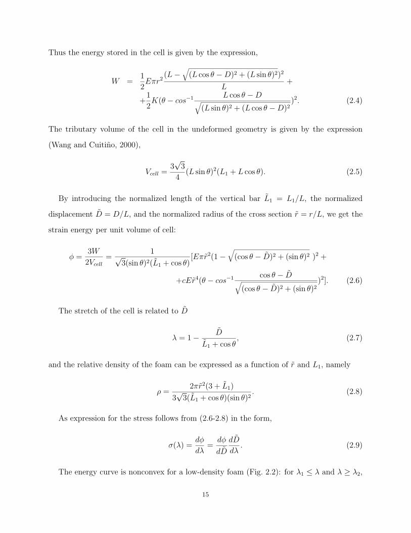
2.2 (a) The stress-stretch curve for a low-density foam. (b) The attendant energy curve, which isnonconvex. . . . . . . . . . . . . . . . . . . . . . . . . . . . . . . . . . . . . . . . . . . . . . . 16

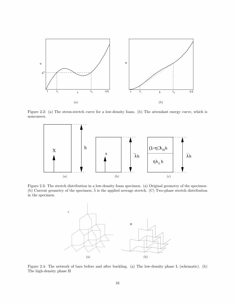
2.3 The stretch distribution in a low-density foam specimen. (a) Original geometry of the speci-men. (b) Current geometry of the specimen; λ is the applied average stretch. (C) Two-phasestretch distribution in the specimen. . . . . . . . . . . . . . . . . . . . . . . . . . . . . . . . . 16

2.4 The network of bars before and after buckling. (a) The low-density phase L (schematic). (b)The high-density phase H . . . . . . . . . . . . . . . . . . . . . . . . . . . . . . . . . . . . . . 16

x

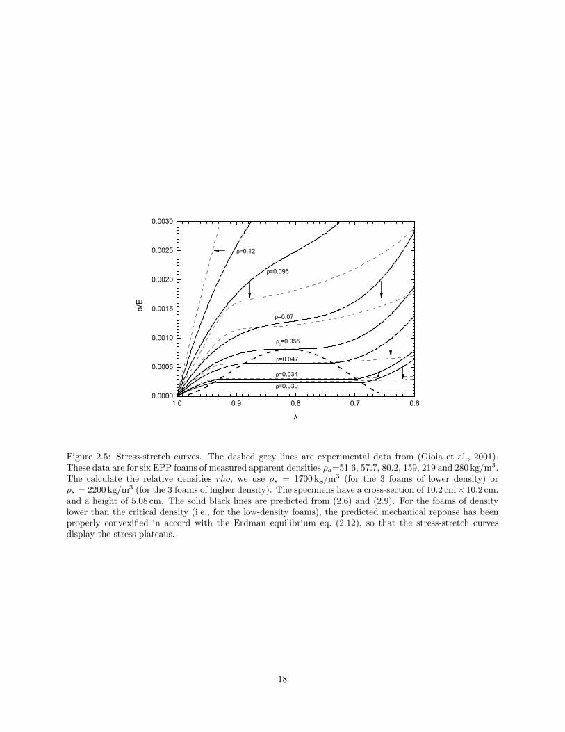
2.5 Stress-stretch curves. The dashed grey lines are experimental data from (Gioia et al., 2001).These data are for six EPP foams of measured apparent densities ρa=51.6, 57.7, 80.2, 159, 219and 280 kg/m3. The calculate the relative densities rho, we use ρs = 1700 kg/m3 (for the 3foams of lower density) or ρs = 2200 kg/m3 (for the 3 foams of higher density). The specimenshave a cross-section of 10.2 cm× 10.2 cm, and a height of 5.08 cm. The solid black lines arepredicted from (2.6) and (2.9). For the foams of density lower than the critical density (i.e.,for the low-density foams), the predicted mechanical reponse has been properly convexified inaccord with the Erdman equilibrium eq. (2.12), so that the stress-stretch curves display thestress plateaus. . . . . . . . . . . . . . . . . . . . . . . . . . . . . . . . . . . . . . . . . . . . . 18

2.6 (a) λL and λH in a region very close to the critical point. (b) λL − λH vs. |ρ− ρc| in log-logscale. . . . . . . . . . . . . . . . . . . . . . . . . . . . . . . . . . . . . . . . . . . . . . . . . . . 20

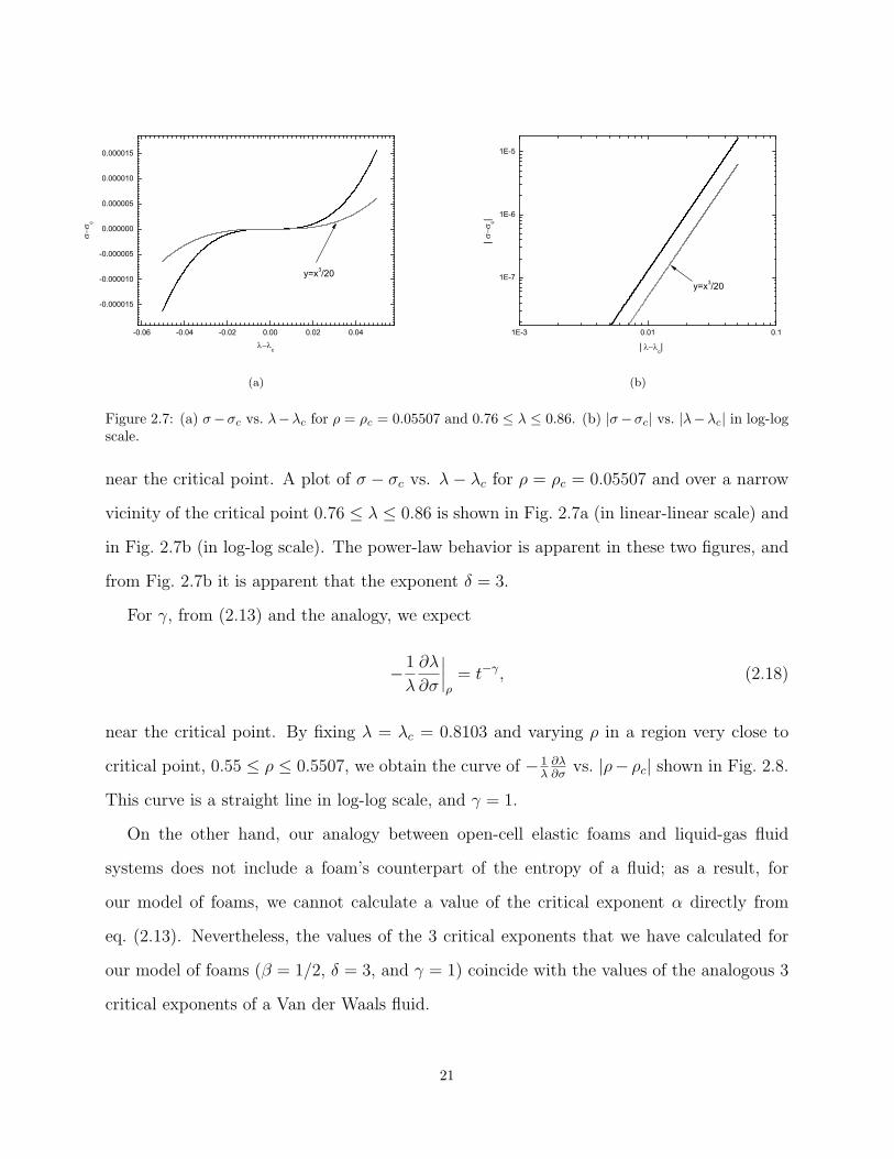
2.7 (a) σ − σc vs. λ − λc for ρ = ρc = 0.05507 and 0.76 ≤ λ ≤ 0.86. (b) |σ − σc| vs. |λ − λc| inlog-log scale. . . . . . . . . . . . . . . . . . . . . . . . . . . . . . . . . . . . . . . . . . . . . . 21

2.8 − 1λ

∂λ∂σ vs. |ρ− ρc| in log-log scale. . . . . . . . . . . . . . . . . . . . . . . . . . . . . . . . . . . 22

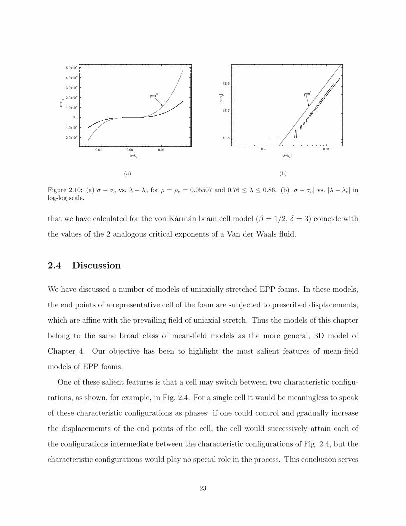
2.9 (a) λH and λL in a region very close to critical point. (b) λH − λL vs. ρ− ρc in log-log scale. 222.10 (a) σ − σc vs. λ − λc for ρ = ρc = 0.05507 and 0.76 ≤ λ ≤ 0.86. (b) |σ − σc| vs. |λ − λc| in

log-log scale. . . . . . . . . . . . . . . . . . . . . . . . . . . . . . . . . . . . . . . . . . . . . . 23

3.1 ATS testing machine setup . . . . . . . . . . . . . . . . . . . . . . . . . . . . . . . . . . . . . 283.2 (a) Photograph of the TurePath Automated Stress Path System. (b) Sketch of the TurePath

Automated Stress Path System. . . . . . . . . . . . . . . . . . . . . . . . . . . . . . . . . . . . 293.3 Stress-strain curves of 6 load-unload cycles, for an EPP foam of relative density ρ = 0.046

subjected to uniaxial compression along the rise direction. . . . . . . . . . . . . . . . . . . . . 313.4 The modulus of foams specimens vs. the density . . . . . . . . . . . . . . . . . . . . . . . . . 323.5 The foam specimen and the frame for global DIC . . . . . . . . . . . . . . . . . . . . . . . . . 343.6 Axial stress vs. axial strain curves of foam specimens of five densities under uniaxial compres-

sion along the rise direction. . . . . . . . . . . . . . . . . . . . . . . . . . . . . . . . . . . . . . 383.7 Axial stress vs. axial strain curve of the low density foam specimen under uniaxial compression

along the rise direction. . . . . . . . . . . . . . . . . . . . . . . . . . . . . . . . . . . . . . . . 393.8 Contours of displacement along the rise direction for the foam of lower density. . . . . . . . . 403.9 Plots of displacements in y direction of points on the foam surface along the dashed line drawn

in Fig. 3.8a, corresponding to strain values of point A to F in Fig. 3.7. . . . . . . . . . . . . . 413.10 Axial stress vs. axial strain curve of the high density foam specimen under uniaxial compres-

sion along the rise direction. . . . . . . . . . . . . . . . . . . . . . . . . . . . . . . . . . . . . . 423.11 Contours of displacement along the rise direction for the foam of higher density under uniaxial

compression along the rise direction. . . . . . . . . . . . . . . . . . . . . . . . . . . . . . . . . 423.12 Axial stress vs. axial strain of foam specimens of five densities for uniaxial compression along

one of the transverse direction . . . . . . . . . . . . . . . . . . . . . . . . . . . . . . . . . . . . 433.13 Axial stress vs. axial strain of the least dense foam specimen for uniaxial compression along

the rise and transverse directions. . . . . . . . . . . . . . . . . . . . . . . . . . . . . . . . . . . 443.14 Displacement field for compression along the transverse direction. . . . . . . . . . . . . . . . . 453.15 (a) Tension test specimen and set up. (b) Sketch of the set up. . . . . . . . . . . . . . . . . . 463.16 Axial stress vs. axial strain of foam specimens of five densities for uniaxial tension along the

rise direction. . . . . . . . . . . . . . . . . . . . . . . . . . . . . . . . . . . . . . . . . . . . . . 463.17 (a) Compression loading test set-up. (b) Sketch of the set up . . . . . . . . . . . . . . . . . . 473.18 Vertical force vs. vertical displacement for foam specimens of five different densities for the

compression and shear combined loading. . . . . . . . . . . . . . . . . . . . . . . . . . . . . . 483.19 Vertical force vs. vertical displacement curves for specimens with dimensions 10 cm × 10 cm

× 10 cm and 10 cm× 10 cm× 5 cm, subjected to compression and shear combined loading. Thedisplacement is normalized by dividing the specimen height. . . . . . . . . . . . . . . . . . . . 49

3.20 Displacement field for compression and shear combined loading of low density foam specimenof size 10 cm× 10 cm× 10 cm . . . . . . . . . . . . . . . . . . . . . . . . . . . . . . . . . . . . 50

xi

3.21 Plots of displacements in the y direction of points on the foam surface along the dashed linedrawn in Fig. 3.20b, corresponding to strain values of point A to F in Fig. 3.19. . . . . . . . . 50

3.22 Vertical force vs. vertical displacement curves for triaxial loading . . . . . . . . . . . . . . . . 513.23 The bulging that occurs during uniaxial compression of a foam specimen of density 50.3 kg/m3

and dimensions 10 cm× 10 cm× 10 cm. The pictures in (a) to (e) are the deformed foamsurface at average stretch (the height of the deformed specimen divided by the original height)of 1 (undeformed), 0.910, 0.790, 0.701, 0.591 and 0.481, respectively . . . . . . . . . . . . . . 54

3.24 The foam specimen and the finite element mesh used for global DIC. . . . . . . . . . . . . . . 543.25 The deformed mesh calculated with global DIC. Figures (a) to (e) correspond to the deformed

foam surfaces (a) to (e) in Fig. 3.23, respectively . . . . . . . . . . . . . . . . . . . . . . . . . 553.26 Contours of constant displacement in the loading direction. The displacement of one contour

differs from the displacement of a contiguous contour by 0.1 cm; the displacement of some ofthe contours are marked (in cm). The contour plot (a) to (e) corresponds to the deformedfoam surface (a) to (e) of Fig. 3.23 respectively . . . . . . . . . . . . . . . . . . . . . . . . . . 56

4.1 The idealized foam representative microstructure. (a) 3D view of the foam microstructure.(b) Front view. (c) Side view. (d) Top view. . . . . . . . . . . . . . . . . . . . . . . . . . . . . 60

4.2 The boundary faces of the substructure . . . . . . . . . . . . . . . . . . . . . . . . . . . . . . 624.3 The deformed substructure under uniaxial loading along the rise direction (a) Front view. (b)

Side view . . . . . . . . . . . . . . . . . . . . . . . . . . . . . . . . . . . . . . . . . . . . . . . 664.4 The experimental and predicted response of foam specimens for uniaxial compression along

the rise direction . . . . . . . . . . . . . . . . . . . . . . . . . . . . . . . . . . . . . . . . . . . 674.5 The deformed substructure under uniaxial loading along the transverse direction (a) Top view.

(b) Side view . . . . . . . . . . . . . . . . . . . . . . . . . . . . . . . . . . . . . . . . . . . . . 684.6 The experimental and predicted response of foam specimens for uniaxial compression along

one of the transverse direction . . . . . . . . . . . . . . . . . . . . . . . . . . . . . . . . . . . . 694.7 The deformed substructure under uniaxial loading along the transverse direction (a) Front

view. (b) Side view . . . . . . . . . . . . . . . . . . . . . . . . . . . . . . . . . . . . . . . . . . 704.8 The experimental and predicted response of foam specimens for Compression-shear combined

loading . . . . . . . . . . . . . . . . . . . . . . . . . . . . . . . . . . . . . . . . . . . . . . . . . 714.9 The experimental and predicted response for uniaxial tension along the rise direction . . . . . 724.10 The normalized axial stress vs axial strain curves for the triaxial loading case (a) For specimen

with relative density ρ = 0.038. (b) For specimen with relative density ρ = 0.046. (c) Forspecimen with relative density ρ = 0.065. (ed) For specimen with relative density ρ = 0.086. . 73

5.1 Experimental setup for wedge-punching . . . . . . . . . . . . . . . . . . . . . . . . . . . . . . 785.2 Plots of the force vs. the penetration displacement measured in five experiments with the

wedge-shaped punch. (a) The three experiments correspond to foams of low densities (EF −4003, EF − 4004, EF − 4005). (b) The two experiments correspond to foams of high densities(TF5070− 10 and TF5070− 13). For comparison, the height of the specimen is 10 cm. . . . 79

5.3 Schematic of a strain field with a smooth transition from a high strain close to the tip of thepunch to a low strain far from the tip. . . . . . . . . . . . . . . . . . . . . . . . . . . . . . . . 80

5.4 Microphotographs of an array of cells in a polyether polyurethane foam and the cap of ashampoo bottle. The cap and a foam cell are examples of bi-stable elastic structures. (a)Plane perpendicular to the rise direction. (b) Plane parallel to the rise direction. (c) AnIdealized array of cells. (d) The array of cells after snap-through buckling. (e) Closed cap.(f) Open cap. . . . . . . . . . . . . . . . . . . . . . . . . . . . . . . . . . . . . . . . . . . . . 82

5.5 Schematic strain field with a sharp transition. (a) 3-D view. (b) Front view. As the penetra-tion increases, the radius of the sharp interface increases proportionally. . . . . . . . . . . . . 82

5.6 DIC frame for wedge punching on a low density (ρ = 0.038) cubic specimen . . . . . . . . . . 845.7 Contours of displacement along the rise direction for the foam of lower density . . . . . . . . 855.8 The normalized force-penetration depth curves for low density cubic foam specimens . . . . . 88

xii

5.9 The curves of loading force vs. the penetration depth for wedge punching on low density foamspecimens with a geometry of a cross section 10 cm× 10 cm and a height of 5.0 cm. (a) Forcevs. indentation depth curves. (b) Normalized curves . . . . . . . . . . . . . . . . . . . . . . . 89

5.10 (a) Conical punching experimental setting. (b) Sketch of the 3-D interface . . . . . . . . . . . 905.11 Conical punching on cubic specimens. (a) Loading force vs. penetration depth curves. (b)

Corresponding normalized curves . . . . . . . . . . . . . . . . . . . . . . . . . . . . . . . . . . 915.12 Conical punching on shorter specimens. (a) Loading force vs. penetration depth curves. (b)

Corresponding normalized curves . . . . . . . . . . . . . . . . . . . . . . . . . . . . . . . . . . 915.13 Loading force vs. penetration depth curve in log-log space for conical punching on short

specimens . . . . . . . . . . . . . . . . . . . . . . . . . . . . . . . . . . . . . . . . . . . . . . . 92

6.1 (a) A free-standing thin film. C1 and C2 are cuts performed for stress analysis. (b) Thesurface stress T acting on the perimeter of C1. (c) The compressive stress induced by T onthe surface of C1. (d) The compressive stress induced by T on the surface of C2. (e) Appliedtraction that gives the same stresses as T . . . . . . . . . . . . . . . . . . . . . . . . . . . . . 98

6.2 A plot of the dimensionless apparent yield stress σya/σy vs. the dimensionless thickness hσy/T .

See eq. (6.1). The points F, R, M, and V are referred to in the text. The size effect of theapparent tensile yield stress reverses from hardening to softening at the point R. . . . . . . . 100

6.3 A plot of the dimensionless quantities s1, s2, and s3 vs. the dimensionless thickness, hσy/T .See eqs. (6.2–6.4). . . . . . . . . . . . . . . . . . . . . . . . . . . . . . . . . . . . . . . . . . . 106

6.4 A plot of the normalized plastic strain at failure in the direction of the applied stress vs. thedimensionless thickness, hσy/T . See eq. (6.6). . . . . . . . . . . . . . . . . . . . . . . . . . . 107

xiii

Part I

Mechanical response of polyether polyurethane foams

under multiaxial stress

1

Chapter 1

Introduction

Solid foams are cellular materials which may be described as numerous cells joined together

to fill space. The cells can consist of bars (open-cell foams) or membranes (closed-cell foams).

Solid foams have been manufactured out of polymers, metals, carbon, graphite and ceramics.

Solid foams also occur in the form of natural materials such as wood, cork, cancellus bone,

sponge, and coral.

Here we concentrate on open-cell, elastic (or “flexible”) polymeric foams, and in particular

on elastic polyether polyurethane foams. We will frequently refer to the foams of this type

as “EPP foams.”

EPP foams are widely employed in engineering applications. For example, in the aero-

nautical industry, EPP foams are among the most commonly used materials in the cores of

sandwich panels. Due to their ability to absorb impact energy at relatively low compressive

stresses, EPP foams are also widely used in packaging to protect fragile products from the

jolts associated with transportation and handling. For the same reason, EPP foams are used

in car seats to provide comfort and safety to passengers.

The first EPP foam was made by Otto Bayer and coworkers in the laboratory in 1941

(Bayer, 1947). Industrial production started in Germany in 1952. Since then, polymeric

foams have been developing steadily to become a large global industry. According to a

report published recently by Global Industry Analysts, Inc. (2008), the worldwide market

of polymeric foams is to reach 20.5 million tons by 2010.

2

(a) (b)

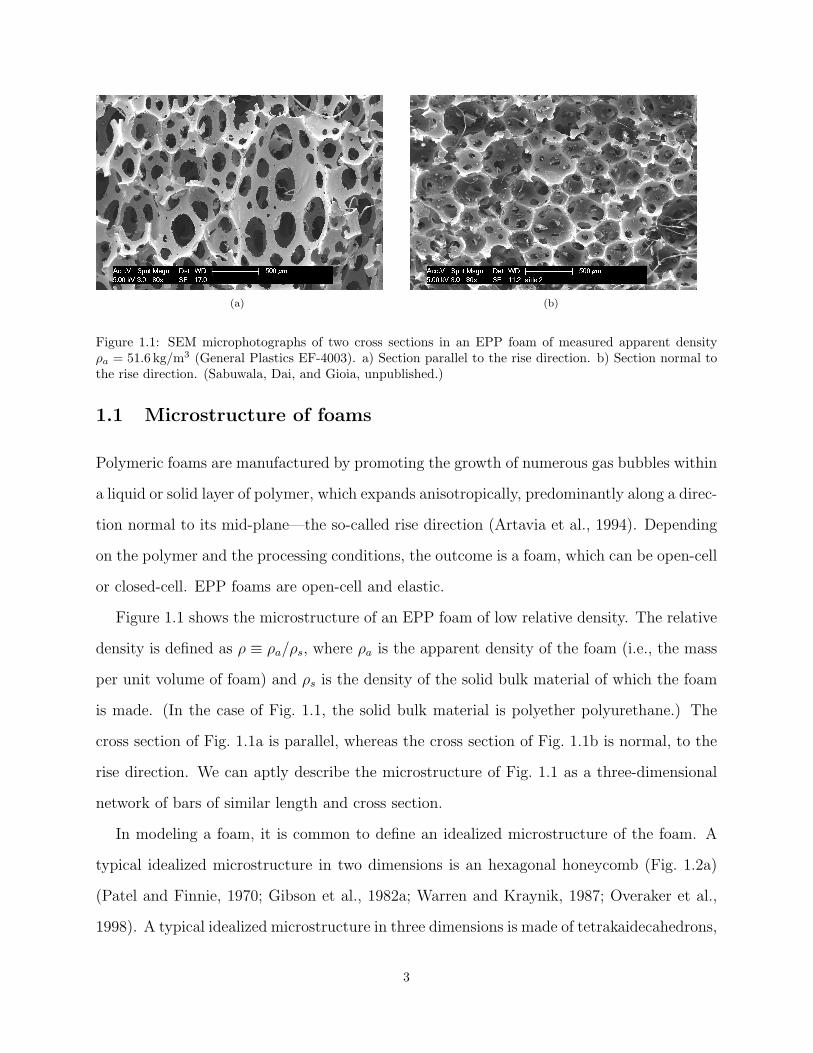
Figure 1.1: SEM microphotographs of two cross sections in an EPP foam of measured apparent densityρa = 51.6 kg/m3 (General Plastics EF-4003). a) Section parallel to the rise direction. b) Section normal tothe rise direction. (Sabuwala, Dai, and Gioia, unpublished.)

1.1 Microstructure of foams

Polymeric foams are manufactured by promoting the growth of numerous gas bubbles within

a liquid or solid layer of polymer, which expands anisotropically, predominantly along a direc-

tion normal to its mid-plane—the so-called rise direction (Artavia et al., 1994). Depending

on the polymer and the processing conditions, the outcome is a foam, which can be open-cell

or closed-cell. EPP foams are open-cell and elastic.

Figure 1.1 shows the microstructure of an EPP foam of low relative density. The relative

density is defined as ρ ≡ ρa/ρs, where ρa is the apparent density of the foam (i.e., the mass

per unit volume of foam) and ρs is the density of the solid bulk material of which the foam

is made. (In the case of Fig. 1.1, the solid bulk material is polyether polyurethane.) The

cross section of Fig. 1.1a is parallel, whereas the cross section of Fig. 1.1b is normal, to the

rise direction. We can aptly describe the microstructure of Fig. 1.1 as a three-dimensional

network of bars of similar length and cross section.

In modeling a foam, it is common to define an idealized microstructure of the foam. A

typical idealized microstructure in two dimensions is an hexagonal honeycomb (Fig. 1.2a)

(Patel and Finnie, 1970; Gibson et al., 1982a; Warren and Kraynik, 1987; Overaker et al.,

1998). A typical idealized microstructure in three dimensions is made of tetrakaidecahedrons,

3

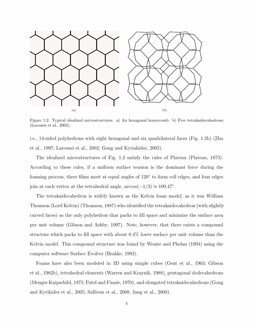
(a) (b)

Figure 1.2: Typical idealized microstructures. a) An hexagonal honeycomb. b) Five tetrakaidecahedrons(Laroussi et al., 2002).

i.e., 14-sided polyhedrons with eight hexagonal and six quadrilateral faces (Fig. 1.2b) (Zhu

et al., 1997; Laroussi et al., 2002; Gong and Kyriakides, 2005).

The idealized microstructures of Fig. 1.2 satisfy the rules of Plateau (Plateau, 1873).

According to these rules, if a uniform surface tension is the dominant force during the

foaming process, three films meet at equal angles of 120◦ to form cell edges, and four edges

join at each vertex at the tetrahedral angle, arccos(−1/3) ≈ 109.47◦.

The tetrakaidecahedron is widely known as the Kelvin foam model, as it was William

Thomson (Lord Kelvin) (Thomson, 1887) who identified the tetrakaidecahedron (with slightly

curved faces) as the only polyhedron that packs to fill space and minimize the surface area

per unit volume (Gibson and Ashby, 1997). Note, however, that there exists a compound

structure which packs to fill space with about 0.4% lower surface per unit volume than the

Kelvin model. This compound structure was found by Weaire and Phelan (1994) using the

computer software Surface Evolver (Brakke, 1992).

Foams have also been modeled in 3D using simple cubes (Gent et al., 1963; Gibson

et al., 1982b), tetrahedral elements (Warren and Kraynik, 1988), pentagonal dodecahedrons

(Menges Knipschild, 1975; Patel and Finnie, 1970), and elongated tetrakaidecahedrons (Gong

and Kyrikides et al., 2005; Sullivan et al., 2008; Jang et al., 2008).

4

1.2 Foam mechanics

Since Gent et al. (1963) proposed one of the first mechanical models of cellular materials,

there has been much research on the mechanics of cellular materials. Gibson and Ashby

(1997) give an extensive review. More detailed studies include the book by Weaire and

Hutzler (1999), and the PhD dissertations of Wang (2001), Daxner (2003) and Gong (2005).

The mechanical models of foams can be divided into two categories. The first category

includes the cell-scale models, which are based on the simplified mechanics of a single,

idealized cell or set of idealized cells. These models relate the structural mechanics of

the cell or set of cells to the mechanical response of an equivalent continuum; both two-

dimensional (Patel and Finnie, 1970; Gibson et al., 1982a; Warren and Kraynik, 1987) and

three-dimensional cell-scale models (Gibson et al., 1982b; Warren and Kraynik, 1988; Zhu et

al., 1997; Wang and Cuitino, 2000; Sullivan et al., 2008) have been proposed. With suitable

boundary conditions, cell-scale models have been used to great advantage. For example,

Gibson and Ashby (1997) have used cell-scale models to identify the relative density as the

most important parameter of foams, and to establish the scaling law that relates the Young’s

modulus of a foam to the relative density of the foam.

The second category includes the statistical models of foams. In these models, a “statis-

tically meaningful” (Schraad and Harlow, 2006) set of cells is used to account for the effect

of irregular foam microstructures. Thus, for example, statistical models have been used by

Papka and Kyriakides to study irregular aluminum honeycombs under uniaxial (1994) and

biaxial (1999a; 1999b) in-plane loading; by Triantafyllidis and Schraad (1998), Chen et al.

(1999), Zhu et al. (2001), Okumura et al. (2004), and Zhu et al. (2006) to ascertain the

deformation mechanism of ideal and Voronoi honeycombs; and by Laroussi et al. (2002) to

study the nonlinear mechanical response of 3D open-cell foams. Other studies of the effect of

irregular foam microstructures have been performed by Zhu et al. (2000) and (2002). More

recently, Gong and Kyriakides (2005) have studied the effects of the shear deformation and

the cross-sectional shape of the struts of open-cell foams. Using X-ray tomography (Maire

5

0.1 0.2 0.3 0.4 0.5

5

10

15

20

25

[kPa]σ

01 0.8 0.6 λ

10

20

Figure 1.3: Mechanical response of the low-density EPP foam of Fig. 1.1 subject to uniaxial compressivestretch along the rise direction (Gioia et al., 2001). A stretch λ = 1 corresponds to the undeformed geometry,whereas stretches λ < 1 correspond to compressed geometries.

et al., 2003), Jang et al. (2008) have been able to ascertain the effect of geometrical details

such as the cell size and ligament length distributions, and the geometry of the nodes.

1.3 Elastic Polyether Polyurethane foams under uniaxial

compressive loading along the rise direction

In this section, we present a brief review of the mechanical response of EPP foams under

uniaxial compressive loading along the rise direction. As part of this brief review, we intro-

duce a number of concepts which will recur throughout the present work, starting from the

following section, in which we state the major goals of the work.

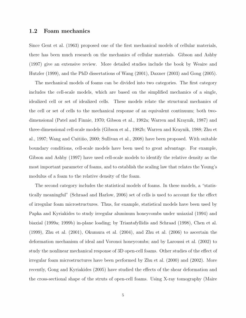
In Fig. 1.3 we show the typical mechanical response of a low-density EPP foam subject

to uniaxial compressive stretch along the rise direction. The stress-stretch (σ-λ) curve of

Fig. 1.3 consists of a linear portion, a stress plateau, and a hardening portion. The most

interesting feature of this σ-λ curve is the stress plateau.

The stress plateau of Fig. 1.3 occurs only in low-density EPP foams. If the density of a

foam is higher than a certain critical density, there is no stress plateau, and the σ-λ curve

hardens monotonically throughout the experiment. Thus the mechanical response of an EPP

foam depends not just quantitatively but qualitatively on the density of the foam.

A crucial point that has frequently been overlooked concerns the stretch (or strain) fields

that accompany a stress plateau. These stretch fields are highly heterogenous (Fig. 1.4).

6

Figure 1.4: Typical displacement field on the surface of a low-density foam. Measured during the uniaxialtest that gave the stress–stretch curve of Fig. 1.3 (Gioia et al., 2001). The foam is the low-density EPP foamof Fig. 1.1, and the applied average stretch is λ = 0.74, within the stress plateau of Fig. 1.3. The surfaceshown in the figure is 3.72 cm× 2.54 cm, and the height of 2.54 cm is aligned with the rise direction, whichcoincides with the X-axis and the direction of loading. The units of X and Y are pixels, and the geometryis the underformed geometry. The displacement field is given in the form of a contour plot. Each contour inthe figure corresponds to a constant value of the displacement uX in the rise direction. The value of uX onany given contour differs by a fixed increment from the value of uX on an adjacent contour. The contours inthe figure indicate the existence of two preferred values of ∂uX/∂X, which correspond to two characteristicvalues of stretch and two configurational phases of the microstructure of the foam (Gioia et al., 2001).

Therefore, the values of λ in Fig. 1.3 must be interpreted as as values of the applied average

(or mean) stretch.

Further, the stretch fields of Fig. 1.4 reveal the existence of two preferred values of stretch.

These preferred values of stretch remain invariant as the σ–λ curve traces the stress plateau.

The changing values of the applied average stretch are accommodated by suitable changes in

the relative volume fraction of the preferred values of stretch. Values of stretch in between

the two preferred values of stretch appear be excluded from the measured stretch fields.

It is widely thought that the stress plateau of Fig. 1.3 is related to a buckling of the

network of bars of Fig. 1.1. A number of authors have proposed that this is conventional,

7

or Euler, buckling—that is to say, bifurcation of equilibrium (Papka and Kyriakides, 1994;

Gong and Kyriakides, 2005). However, the buckling process has been documented at the

microstructural level by Gioia et al. (2001) (Fig. 1.5), who concluded that the microstructure

undergoes snap-through buckling, a limit-point phenomenon without bifurcation of equilib-

rium.

If the microstructure of a foam undergoes Euler buckling, the attendant stretch field will

correspond to an eigenfunction of arbitrary amplitude. As the applied average stretch is

decreased following buckling, the stress-stretch curve traces a stress plateau, and the stretch

field remains invariant except for the amplitude, which increases to accommodate the applied

average stretch. Thus the mechanism of Euler buckling does not appear to be consistent with

the observed stretch fields, where two preferred values of stretch are present in association

with the stress plateau, and intermediate values of stretch are excluded.

Where a cell of a low-density EPP foam undergoes snap-through buckling, the cell

switches discontinuously between a geometric configuration associated with a characteristic,

high value of stretch (or low value of strain) to a geometrical configuration associated with

a characteristic, low value of stretch (or high value of strain). Therefore, the cell behaves

as a bistable elastic structure, and the two characteristic values of stretch (or strain) can

be identified with the two preferred values of stretch observed in experiments, and ascribed

to two distinct configurational phases of the foam. The heterogenous stretch fields observed

in experiments are two-phase fields. In these two-phase fields, the applied average stretch

is accommodated by mixing the two configurational phases of the foam in accord with the

rule of mixtures. The stress plateau corresponds to a Maxwell stress.

We conclude that the mechanism of snap-through buckling provides a straightforward

theoretical interpretation of the stretch fields and the stress plateau observed in experiments

Gioia et al. (2001). In this interpretaion, the basic physics of large deformation in low-density

EPP foams is the physics of phase transitions.

8

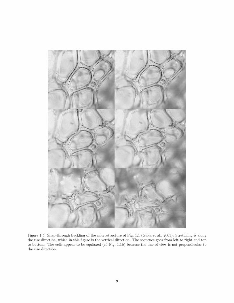
Figure 1.5: Snap-through buckling of the microstructure of Fig. 1.1 (Gioia et al., 2001). Stretching is alongthe rise direction, which in this figure is the vertical direction. The sequence goes from left to right and topto bottom. The cells appear to be equiaxed (cf. Fig. 1.1b) because the line of view is not perpendicular tothe rise direction.

9

1.4 Statement of the major goals of this research

In spite of much research into the mechanical behavior of elastic foams, much remains to be

done, and the state of the art in models of elastic foams is far from satisfactory.

1. Most practical applications of foams involve multiaxial loading, but there has been

little experimental and theoretical work on the mechanical response of elastic foams

subjected to multiaxial states of stress. In particular, there is a need for a model capable

of predicting the mechanical response of elastic foams under arbitrary triaxial states

of stress. Such a model must be calibrated by comparison with suitable experimental

measurements of the mechanical response of elastic foams under multiaxial state of

stress.

2. The mechanical response of an elastic foam depends not just quantitatively but also

qualitatively on the relative density of the foam. Yet no model has been used to make

predictions for sets of foams of widely differing densities, and calibrated using experi-

mental measurements for a complete series of commercially available elastic foams.

3. The scant comparisons with experiments have been limited to the value of the stress

plateau, and no model has been tested over the entire mechanical response as a function

of the strain, and for widely differing densities.

4. A stress plateau appears to be invariably accompanied by heterogeneous, two-phase

strain fields, yet little attention has been paid to whether a model is capable of predicting

heterogenous two-phase strain fields.

Here we investigate the deformation mechanism of open-cell elastic foams, more specifi-

cally elastic polyether polyurethane (EPP) foams, by means of theory, experiments and com-

putations. In applications, under service conditions, EPP foams are commonly subjected

to large strains, in a regime where nonlinear geometrical effects dominate the mechanical

response. Therefore, the mechanical behavior of EPP foams under large strains is of special

interest to us, and the mechanical response under small strains of relatively minor interest.

10

Our main goal is to develop and calibrate a model of EPP foams capable of addressing

points 1 to 4 above. A crucial component of this endeavor is to obtain suitable experimental

data for the purpose of calibrating the model. The experimental data must include stress–

strain or force–displacement curves for a variety of loading conditions and foam densities,

as well as full strain fields, which will allow us to ascertain the character of the strain fields

associated with a given loading condition.

Thus, as part of the calibration of our model, we will verify not just that the model

predict a stress plateau where a stress plateau has been observed in experiments, but also

that the model predict the two-phase strain fields associated with a stress plateau. To this

end, the model must embody the basic physics of large-strain deformation in EPP foms: the

physics of phase transitions.

In the chapter that follows (Chapter 2), we seek to provide a suitable theoretical frame-

work for our research. To that end, we discuss a few mean-field models of EPP foams.

The class of mean-field models is the class to which our model of Chapter 4 belongs, but

in Chapter 2 we focus on foams subjected to uniaxial loading and discuss a number of

specialized versions of our model of Chapter 4. These specialized versions of our model

of Chapter 4 afford us an opportunity to highlight the two most salient characteristics of

mean-field models in general: that, in accord with experimental results, these models may

undergo configurational phase transitions and exhibit a critical point.

11

Chapter 2

Uniaxial mean-field models and thecritical point

2.1 Introduction

It has been shown experimentally that where an elastic polyether polyurethane (EPP) foam

of relatively low density is compressed along the rise direction, the foam displays two pre-

ferred values of stretch which may be interpreted as configurational phases of the microstruc-

ture of the foam (Gioia et al., 2001). If a foam of higher density is compressed, the two

preferred values of stretch are closer together, and there exists a critical density for which

the two preferred values of stretch coincide at a critical point.

In thermodynamics, the critical point is the apex of a coexistence curve which separates

two distinct phases. Above the critical point, it is possible to pass from one phase to the

other without discontinuities (Goldenfeld, 1992). Power-law behavior governs second-order

phase transitions (also called continuous phase transitions) in the immediate vicinity of a

critical point (Goldenfeld, 1992), and the exponents that appear in the power laws are known

as critical exponents. For example, experiments indicate that in the liquid-gas transition of

sulphur hexafluoride (SF6),

| ρ+ − ρ− |∝| T − Tc |0.327±0.006 (2.1)

near critical point, where T is the temperature, Tc is the critical temperature, ρ+ and ρ−

are the values of the density on the two branches of the coexistence curve below Tc—that is

to say, the preferred values of density, and 0.327± 0.006 is the critical exponent. Similarly,

experiments indicate that at the onset of magnetization in the antiferromagnet DyAlO3, the

12

magnetization behaves in the form:

M ∝ (Tc − T )0.311±0.005. (2.2)

The critical exponents are frequently found to be independent of the specific system, a

phenomenon known as universality (Goldenfeld, 1992). For example, for SF6 and DyAlO3

the exponents are the same within experimental resolution.

It is virtually impossible for us to study the critical point of EPP foams experimentally,

because EPP foams are not available in any given relative density. In this chapter, we will

use theoretical models to investigate the mechanical behavior of EPP foams close to the

critical point.

2.2 A simplified mean-field model

Compressed open-cell solid foams frequently exhibit spatially heterogeneous distributions of

local stretch. Gioia et al. (2001) proposed a mean-field model and studied the energetics

of the model to show that the stretch heterogeneity observed in uniaxial experiments stems

from the lack of convexity of the governing energy functional, which favors two characteristic

values of local stretch. These characteristic values of the local strech are independent of the

applied average stretch and define two configurational phases of the foam. The predicted

stretch distributions correspond to stratified mixtures of the phases; stretching occurs in the

form of a phase transition, by growth of the volume fraction of one of the phases at the

expense of the volume fraction of other (Gioia et al., 2001).

The mean-field model of Gioia et al. (2001) yields predictions that are in good accord

with experimental data for a series of EPP foams of relative densities ranging from 0.03

to 0.12. Nevertheless, in this model the microstructure of the foam is a regular network

of bars governed by the von Karman theory of beams, and the mechanical response must

be calculated computationally. Here we introduce a simplified mean-field model (Dai and

Gioia, 2008) for which the mechanical response can be calculate analytically.

13

Rise

(b)

(c)

F

D

L

L1

L1

L

(a)

θ

θ

Direction

Figure 2.1: The simplified mean-field model of EPP foams. (a) Undeformed network of bars. (b) A four-barcell. (c) For uniaxial stretch along the rise direction, the four-bar cell may be thought of as a two-bar cell.

In our model, the foam is a regular network of bars (Fig. 2.1a) made of identical four-bar

tetrahedral cells. In each one of these four-bar tetrahedral cells, a bar of length L1 is aligned

with the rise direction of the foam. This bar is rigid. The other three bars, of length L and

circular cross section of radius r, form an angle θ with the rise direction (Fig. 2.1b). These

bars are linear elastic, have a Young’s modulus E, and can only deform axially, without

bending. If the foam is stretched uniaxially along the rise direction, the four-bar cell may

be thought of as a two-bar cell (Fig. 2.1c).

To endow this two-bar cell with bending energy, we add a rotational spring of modulus

K, so that the bending energy of the cell is given by the expression, Wb = 12K(∆θ)2. We

use K = cEr4/L (from the relation between a moment and the attendant rotation angle in

a beam), where c is a dimensionless parameter and can be viewed as a material property of

the foam.

The relation between the change of angle ∆θ and the displacement D of the upper node

is set by the geometry:

∆θ = θ − cos−1 L cos θ −D√(L sin θ)2 + (L cos θ −D)2

. (2.3)

14

Thus the energy stored in the cell is given by the expression,

W =1

2Eπr2

(L−√

(L cos θ −D)2 + (L sin θ)2)2

L+

+1

2K(θ − cos−1 L cos θ −D√

(L sin θ)2 + (L cos θ −D)2)2. (2.4)

The tributary volume of the cell in the undeformed geometry is given by the expression

(Wang and Cuitino, 2000),

Vcell =3√

3

4(L sin θ)2(L1 + L cos θ). (2.5)

By introducing the normalized length of the vertical bar L1 = L1/L, the normalized

displacement D = D/L, and the normalized radius of the cross section r = r/L, we get the

strain energy per unit volume of cell:

φ =3W

2Vcell

=1√

3(sin θ)2(L1 + cos θ)[Eπr2(1−

√(cos θ − D)2 + (sin θ)2 )2 +

+cEr4(θ − cos−1 cos θ − D√(cos θ − D)2 + (sin θ)2

)2]. (2.6)

The stretch of the cell is related to D

λ = 1− D

L1 + cos θ, (2.7)

and the relative density of the foam can be expressed as a function of r and L1, namely

ρ =2πr2(3 + L1)

3√

3(L1 + cos θ)(sin θ)2. (2.8)

As expression for the stress follows from (2.6-2.8) in the form,

σ(λ) =dφ

dλ=

dφ

dD

dD

dλ. (2.9)

The energy curve is nonconvex for a low-density foam (Fig. 2.2): for λ1 ≤ λ and λ ≥ λ2,

15

σ p

λH

λL

σ

λ1 0.5

(a)

λ λH

λL

φ

1 0.5

(b)

Figure 2.2: (a) The stress-stretch curve for a low-density foam. (b) The attendant energy curve, which isnonconvex.

Xh

(a)

λxh

(b)

H

hλλLη

λ(1−η) h

h

(c)

Figure 2.3: The stretch distribution in a low-density foam specimen. (a) Original geometry of the specimen.(b) Current geometry of the specimen; λ is the applied average stretch. (C) Two-phase stretch distributionin the specimen.

L

(a)

H

(b)

Figure 2.4: The network of bars before and after buckling. (a) The low-density phase L (schematic). (b)The high-density phase H

16

the curvature is positive, d2φdλ2 > 0, whereas for λ1 < λ < λ2 the curvature is negative, d2φ

dλ2 < 0.

A homogeneous strain distribution cannot be realized when the applied average stretch λ is

in the range (λ1, λ2). Thus a heterogeneous stretch distribution should occur (Fig. 2.3).

Assume that a volume fraction η is under a stretch λL > λ and the volume fraction 1− η

is under a stretch λH < λ. (The stretches λL and λH correspond to the unbuckled and

buckled phases of Fig. 2.4, respectively.) For compatibility with the applied average stretch

λ, we must satisfy the rule of mixtures,

η =λL − λ

λL − λH

. (2.10)

The average energy density of the specimen is then a function of λL, λH and η,

φ∗(λL, λH , η) = ηφ(λH) + (1− η)φ(λL). (2.11)

The equilibrium can be realized by making φ∗(λL, λH , η) stationary subject to the sub-

sidiary condition (2.10). Then, λL, λH , and the plateau stress σp (which is a Maxwell stress)

follow from the Erdmann equilibrium equations (Gioia et al., 2001),

σp = −φ(λL)− φ(λH)

λL − λH

= −φ′(λ)|λ=λL= −φ′(λ)|λ=λH

. (2.12)

Associated with the stress plateau, a two-phase stretch distribution exists for each value

of overall stretch in the range λL ≥ λ ≥ λH . When λ decreases from λL to λH , the volume

fraction of the unbuckled phase, η, changes from 0 to 1 and the stress remains constant. Thus

a decrease of the overall stretch λ is accompanied by the propagation of the interface which

separates the two phases. This process is analogous to the transition of a material from

the liquid phase to the gaseous phase: as the liquid/gas interface propagates, the pressure

remains constant.

Equation 2.12 gives λL and λH for low-density foams. As the foam density increases, λL

gets closer to λH ; where ρ attains a critical value ρc, then λL = λH , the two configurational

17

1.0 0.9 0.8 0.7 0.60.0000

0.0005

0.0010

0.0015

0.0020

0.0025

0.0030

ρ=0.030

ρ=0.034

ρ=0.047

ρc=0.055

ρ=0.07

ρ=0.096

ρ=0.12

σ/E

λ

Figure 2.5: Stress-stretch curves. The dashed grey lines are experimental data from (Gioia et al., 2001).These data are for six EPP foams of measured apparent densities ρa=51.6, 57.7, 80.2, 159, 219 and 280 kg/m3.The calculate the relative densities rho, we use ρs = 1700 kg/m3 (for the 3 foams of lower density) orρs = 2200 kg/m3 (for the 3 foams of higher density). The specimens have a cross-section of 10.2 cm× 10.2 cm,and a height of 5.08 cm. The solid black lines are predicted from (2.6) and (2.9). For the foams of densitylower than the critical density (i.e., for the low-density foams), the predicted mechanical reponse has beenproperly convexified in accord with the Erdman equilibrium eq. (2.12), so that the stress-stretch curvesdisplay the stress plateaus.

18

phases are not distinguishable, and we have reached the critical point. For foams of density

higher than ρc, there is no phase transition and hence no stress plateau. By choosing

θ = cos−1(1/3), L1 = 1.5, c = 10.2, and E = 42 MPa, we obtain a good fit of the experimental

data of Gioia et al. (2001) (Fig. 2.5). The critical point is apparent in Fig. 2.5; the critical

density, critical stress, and critical stretch associated with this critical point are ρc = 0.5507,

σc = 7.8591× 10−4Em, and λc = 0.8103, respectively.

2.3 Critical exponents

For liquid-gas fluid systems that are describable by the pressure p, the specific volume v,

and the absolute temperature T , the following power-law relations hold close to the critical

point:v − vc

vc

∼ |t|β;p− pc

pc

∼ (v − vc

vc

)δ

;

Cv = T∂S

∂T= tα; KT ≡ 1

v

∂v

∂p

∣∣∣∣Tt−γ,

(2.13)

where pc is the critical pressure, vc is the critical specific volume, and Tc is the critical

temperature respectively, t ≡ (T − Tc)/Tc, S is the entropy, KT is the compressibility at

constant temperature, Cv is the specific heat capacity at constant volume, and α, β, δ and

γ are critical exponents.

Van der Waals proposed an equation of state for the liquid-gas fluid system:

p =kBT

v − b− a

v2, (2.14)

where a and b are two constants depending on the fluid system. The Van der Walls equation

of state accounts for the hard core potential of the atoms (i.e. the excluded volume) and the

attractive interactions between the atoms.

From (2.13) and (2.14), the critical exponents of Van der Waals fluids can be calculated

analytically, and it is found that β = 1/2, δ = 3, α = 0, γ = 1 (Goldenfeld, 1992).

The experimental results of Fig. 2.5 suggest an analogy (Gioia et al., 2001) between

19

-0.00004 -0.00003 -0.00002 -0.00001 0.00000 0.00001

0.805

0.806

0.807

0.808

0.809

0.810

0.811

0.812

0.813

0.814

0.815

0.816

λΗ

λL

λ

ρ−ρc

(a)

1E-7 1E-6 1E-5 1E-4

1E-3

0.01

|ρ−ρc|

λ L−λΗ

y=x1/2

(b)

Figure 2.6: (a) λL and λH in a region very close to the critical point. (b) λL − λH vs. |ρ − ρc| in log-logscale.

open-cell elastic foams and liquid-gas fluid systems. In this analogy

σ ∼ p, λ ∼ v, ρ ∼ T. (2.15)

2.3.1 Critical exponents for the simplified mean-field model

From eq. (2.13) and the analogy, we expect

(λL − λH) ∼ (ρ− ρc)β, (2.16)

near the critical point, where λL and λH are the two preferred stretches, which for the

simplified mean-field foam model can be calculated from eq. (2.12).

In Fig. 2.6a we plot λL and λH over a narrow vicinity of the critical point, 0.550 ≤ ρ ≤0.551. A log-log plot of λL − λH vs. |ρ − ρc| is shown in Fig. 2.6b. From Fig. 2.6b, it is

apparent that β = 1/2.

From eq. (2.13) and the analogy, we expect

σ − σc

σc

∼ (λ− λc

λc

)δ (as ρ = ρc), (2.17)

20

-0.06 -0.04 -0.02 0.00 0.02 0.04

-0.000015

-0.000010

-0.000005

0.000000

0.000005

0.000010

0.000015

y=x3/20

c

c

(a)

1E-3 0.01 0.1

1E-7

1E-6

1E-5

y=x3/20

| c|

|c|

(b)

Figure 2.7: (a) σ−σc vs. λ−λc for ρ = ρc = 0.05507 and 0.76 ≤ λ ≤ 0.86. (b) |σ−σc| vs. |λ−λc| in log-logscale.

near the critical point. A plot of σ − σc vs. λ− λc for ρ = ρc = 0.05507 and over a narrow

vicinity of the critical point 0.76 ≤ λ ≤ 0.86 is shown in Fig. 2.7a (in linear-linear scale) and

in Fig. 2.7b (in log-log scale). The power-law behavior is apparent in these two figures, and

from Fig. 2.7b it is apparent that the exponent δ = 3.

For γ, from (2.13) and the analogy, we expect

−1

λ

∂λ

∂σ

∣∣∣∣ρ

= t−γ, (2.18)

near the critical point. By fixing λ = λc = 0.8103 and varying ρ in a region very close to

critical point, 0.55 ≤ ρ ≤ 0.5507, we obtain the curve of − 1λ

∂λ∂σ

vs. |ρ− ρc| shown in Fig. 2.8.

This curve is a straight line in log-log scale, and γ = 1.

On the other hand, our analogy between open-cell elastic foams and liquid-gas fluid

systems does not include a foam’s counterpart of the entropy of a fluid; as a result, for

our model of foams, we cannot calculate a value of the critical exponent α directly from

eq. (2.13). Nevertheless, the values of the 3 critical exponents that we have calculated for

our model of foams (β = 1/2, δ = 3, and γ = 1) coincide with the values of the analogous 3

critical exponents of a Van der Waals fluid.

21

1E-7 1E-6 1E-510000

100000

1000000

1E7

1E8

y=1/x

ρ−ρc

−1/λ

dλ/d

σ

Figure 2.8: − 1λ

∂λ∂σ vs. |ρ− ρc| in log-log scale.

0.0690 0.0692 0.0694 0.0696 0.0698 0.0700

0.775

0.780

0.785

0.790

0.795

0.800

0.805

λ

ρ

λL

λΗ

(a)

1E-6 1E-5 1E-4 1E-3

1E-3

0.01

λ L−λΗ

|ρ−ρc|

y=x1/2

(b)

Figure 2.9: (a) λH and λL in a region very close to critical point. (b) λH − λL vs. ρ− ρc in log-log scale.

2.3.2 Critical exponents for a Karman-beam mean-field model

For Gioia’s (2001) model, we find the critical point σC = 0.0014105 and λc = 0.78823. The

corresponding critical density is ρc = 0.069673.

We plot λL and λH in Fig. 2.9a over a narrow vicinity of the critical point. A log-log plot

of λL − λH vs. |ρ− ρc| is shown in Fig. 2.9b. From Fig. 2.9b, it is apparent that β = 1/2.

A plot of σ − σc vs. λ − λc for ρ = ρc and over a narrow vicinity of the critical point

is shown in Fig. 2.10a (in linear-linear scale) and in Fig. 2.10b (in log-log scale). From

Fig. 2.10b, it is apparent the exponent δ = 3. Again, the values of the 2 critical exponents

22

-0.01 0.00 0.01

-2.0x10-6

-1.0x10-6

0.0

1.0x10-6

2.0x10-6

3.0x10-6

4.0x10-6

5.0x10-6

σ−

σ c

λ−λc

y=x3

(a)

1E-3 0.01

1E-8

1E-7

1E-6

|σ−σ

c|

|λ−λc|

y=x3

(b)

Figure 2.10: (a) σ − σc vs. λ − λc for ρ = ρc = 0.05507 and 0.76 ≤ λ ≤ 0.86. (b) |σ − σc| vs. |λ − λc| inlog-log scale.

that we have calculated for the von Karman beam cell model (β = 1/2, δ = 3) coincide with

the values of the 2 analogous critical exponents of a Van der Waals fluid.

2.4 Discussion

We have discussed a number of models of uniaxially stretched EPP foams. In these models,

the end points of a representative cell of the foam are subjected to prescribed displacements,

which are affine with the prevailing field of uniaxial stretch. Thus the models of this chapter

belong to the same broad class of mean-field models as the more general, 3D model of

Chapter 4. Our objective has been to highlight the most salient features of mean-field

models of EPP foams.

One of these salient features is that a cell may switch between two characteristic configu-

rations, as shown, for example, in Fig. 2.4. For a single cell it would be meaningless to speak

of these characteristic configurations as phases: if one could control and gradually increase

the displacememts of the end points of the cell, the cell would successively attain each of

the configurations intermediate between the characteristic configurations of Fig. 2.4, but the

characteristic configurations would play no special role in the process. This conclusion serves

23

to stress a key element of our models, namely homogenization, whereby the strain energy of

the cell is used to compute the strain energy density of an equivalent continuum. Any given

portion of the equivalent continuum stands for very many identical cells of the microstruc-

ture of the foam. As a result, where the equivalent continuum is subject to a an applied

stretch, the individual cells that underly the equivalent continuum are free to accommodate

the applied stretch in a number of ways. It is on this freedom inherent in the equivalent

continuum that the energy analysis of (2.10–2.12) hinges upon. In high-density foams the

strain-energy density is convex, the energy analysis selects a unimodal distribution of the

local stretch, and the stretch field is homogeneous. In low-density foams, the strain-energy

density is nonconvex, the energy analysis selects a bimodal distribution of local stretch, and

the stretch field is heterogeneous and composed of two configurational phases.

Nonconvex strain-energy curves, and the attendant configurational phases and two-phase

stretch fields, are not peculiar to mean-field models of uniaxially stretched EPP foams. As

we shall show in Chapter 4, the strain-energy curves accompanying stretch tensors with

at least one compressive component are generally nonconvex; and the calibration of our

model of Chapter 4 will include an unprecedented constraint, that the model should predict

two-phase fields in accord with the experimental results of Chapter 3.

The other salient characteristic of mean-field models of EPP foams is the critical point.

The critical point corresponds to a critical density of the foam. For a foam of critical density,

both the first derivative and the second derivative of the strain-energy curve vanish at the

critical point.

On the basis of a straightforward analogy with a liquid-gas fluid system, we have been able

to compute three critical exponents for a number of mean-field models of uniaxially stretched

EPP foams, and to verify that these critical exponents are the same as the corresponding

critical exponents of a Van der Waals fluid (the classical mean-field model). Although in our

analogy the density of a foam acts as the counterpart of the temperature of a a Van der Waals

fluid fluid, it is presently unclear to us what quantity might act as a foam’s counterpart of

the entropy of a Van der Waals fluid. It may be possible to identify a suitable “effective

24

entropy” of elastic foams, just as researchers have been able to identify a suitable effective

entropy of granular systems (Mehta and Edwards, 1989; Makse and Kurchan, 2002; Coniglio

et al., 2005).

25

Chapter 3

Experiments

In this chapter we report experimental results for a series of elastic polyether polyurethane

(EPP) foams under uniaxial and multiaxial loading. We measure the mechanical response in

terms of stress-strain or force-displacement data. For some loading cases and load densities,

we use a digital image correlation (DIC) technique to track the evolution of the strain field

on a surface of the foam specimen.

3.1 Introduction

Experimental research into the mechanical behavior of polymeric foams has been focused

on two subjects. (1) The elastic properties, which are of limited interest in applications,

where large strains are typically attained under service conditions; and (2) The mechanical

response under uniaxial stress and up to large strains. (See, e.g. Gibson et al. (1982a),

Gibson et al. (1982b), Zhu et al. (1997), Gioia et al. (2001), Gong (2005).)

Experiments with polymeric foams under multiaxial stress have been largely aimed at

mapping the failure envelope in stress space of rigid (or “brittle”) polymeric foams (e.g.

Shaw and Sata (1966) for rigid polysterene foams; Zaslawsk (1973), Maji et al. (1995), and

Triantafillou et al. (1989) for rigid polyurethane foams; Zhang et al. (1997), Deshpande

et al. (2001), and Gdoutos et al. (2002) for rigid PVC foams; and Viot (2009) for rigid

polypropylene foams). This failure envelope is also known by the name of yield envelope.

This name may appear confusing, but rigid polymeric foams often undergo a progressive form

of brittle failure when tested under compression. In this progressive form of brittle failure,

a large deformation accumulates at a constant value of stress, which may be construed as

26

an apparent yield stress.

For EPP foams, extensive multiaxial tests (including uniaxial, biaxial, and hydrostatic

tests) have been performed by Triantafillou et al. (1989). The purpose of these tests was

to trace the yield envelope in stress space. Here the word “yield” refers to the beginning of

the stress plateau that is characteristic of the stress–strain curves of some EPP foams tested

under compression. As this stress plateau occurs only in low-density EPP foams, all of the

foams tested by Triantafillou et al. (1989) were of very low apparent density (or weight per

unit volume of foam), namely 14.3, 21.8, 28, 41.5, 51.6 kg/m3. Only a few stress–strain curves

were published, to illustrate the method whereby the yield stress was extracted from the

stress–strain curves. Thus, despite the importance of multiaxial loading in many practical

applications of EPP foams, there exist no experimental data on the mechanical response

of EPP foams under a variety of loading conditions and for the full range of commercially

available relative densities.

Our purpose here is to conduct an extensive experimental study of the mechanical behav-

ior of EPP foams of a broad range of relative densities, for a variety of loading conditions and

up to large strains. To this end, we use a series of commercially available EPP foams of five

densities ranging from 50.3 to 220.5 kg/m3. We subject each foam to five different loading

cases, namely, uniaxial compression along the rise direction; uniaxial compression along two

mutually perpendicular transverse directions (both normal to the rise direction); uniaxial

tension along the rise direction; biaxial loading which combines shear and compression along

the rise direction and triaxial loading which combines hydrostatic pressure with compression

along the rise direction. In addition to the stress-strain response, for some foam densities

and loading cases we also obtain the strain field on the surface of the foam specimen using

a global digital image correlation (global DIC) technique (Gao et al., 2002).

27

Foam Specimen

Upper Platen

Lower Platen

Digital Camera

Load Cell

Position Transducer

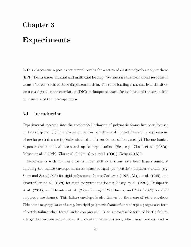
Figure 3.1: ATS testing machine setup

3.2 Experimental set-ups

We use an ATS testing machine (Universal Testing Machines 900 Series, from Applied Test

Systems, Inc.) to conduct tests for the first four loading cases. For the triaxial tests, we use

a TurePath Automated Stress Path System (From GEOTAC).

The ATS testing machine is shown in Fig. 3.1. For the compression tests, the lower plate

is driven up at adjustable rates and compresses the specimen against the fixed upper plate.

The loading force is recorded by a load cell (Interface 100 lbs and 10,000 lbs) attached to the

upper plate while the displacement is measured by a position transducer (PNL022-00 from

Spaceage Control Inc.) attached to the lower plate. During the test, a digital monochrome

CCD camera (PULNiX TM-1300 progressive scan) with NaVITAR Zoom 700 lens can be

used to obtain 8-bit digital images of 1300 by 1030 pixels for DIC analysis.

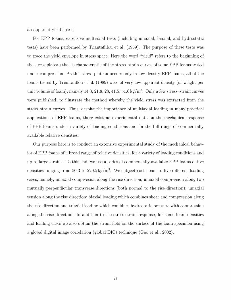
For the triaxial case, the specimen is loaded in a two-step process using the TruePath

Automated Stress Path System (Fig. 3.2a). First, the specimen is immersed in a chamber

filled with silicon oil (Dow Cornings 200 silicone oils, 50cSt). An oil-proof membrane wrapped

around the specimen keeps the specimen dry, while the surrounding oil provides confinement

pressure. To obtain low confinement pressures (2− 10 KPa) we simply change the elevation

of an oil reservoir connected to the oil in the chamber through a thin tube. To obtain higher

confinement pressures we use an oil pump. The lower plate can be driven up by a stepping

28

(a)

����������������������������

���������������������������������������

���������������������������������������

Load Cell(Internal) Platen

Foam Specimen

Silicon Oil(External) Load Cell

Chamber

(b)

Figure 3.2: (a) Photograph of the TurePath Automated Stress Path System. (b) Sketch of the TurePathAutomated Stress Path System.

motor, providing uniaxial compression along the rise direction. The corresponding load is

measured by an internal load cell (Interface 300 lbs range).

We use a series of five EPP foams of apparent density (mass per unit volume of foam)

50.3, 63.0, 77.0, 162.9 and 220.5 kg/m3. These foams are known to the manufacturer, General

Plastics of Tacoma, WA, by the codes EF-4003, EF-4004, EF-4005, TF5070-10 and TF5070-

13 respectively. The relative density ρ is defined as the apparent density ρa of the specimen

divided by the density ρs of the base material. For the EF series, ρs = 1700 kg/m3 whereas for

the TF series ρs = 2540 kg/m3. Thus the relative density is ρ = 0.030, 0.038, 0.046, 0.065,

and 0.086 respectively for the EF-4003, EF-4004, EF-4005, TF5070-10 and TF5070-13 foam.

3.2.1 Error estimation

In our tests, we measure the force F with load cells and the displacement d with a transducer.

For the purpose of error estimation, we consider a single characteristic length of the specimen,

L, which is measured with a ruler. We define the axial stress as σ = F/L2, and the

propagation of errors gives

∆σ = |1/L2|∆F + |2F/L3|∆L.

29

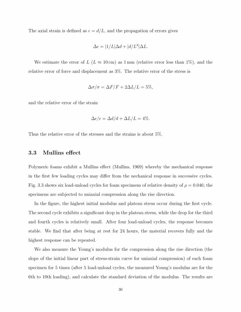
The axial strain is defined as ε = d/L, and the propagation of errors gives

∆ε = |1/L|∆d + |d/L2|∆L.

We estimate the error of L (L ≈ 10 cm) as 1 mm (relative error less than 1%), and the

relative error of force and displacement as 3%. The relative error of the stress is

∆σ/σ = ∆F/F + 2∆L/L = 5%,

and the relative error of the strain

∆ε/ε = ∆d/d + ∆L/L = 4%.

Thus the relative error of the stresses and the strains is about 5%.

3.3 Mullins effect

Polymeric foams exhibit a Mullins effect (Mullins, 1969) whereby the mechanical response

in the first few loading cycles may differ from the nechanical response in successive cycles.

Fig. 3.3 shows six load-unload cycles for foam specimens of relative density of ρ = 0.046; the

specimens are subjected to uniaxial compression along the rise direction.

In the figure, the highest initial modulus and plateau stress occur during the first cycle.

The second cycle exhibits a significant drop in the plateau stress, while the drop for the third

and fourth cycles is relatively small. After four load-unload cycles, the response becomes

stable. We find that after being at rest for 24 hours, the material recovers fully and the

highest response can be repeated.

We also measure the Young’s modulus for the compression along the rise direction (the

slope of the initial linear part of stress-strain curve for uniaxial compression) of each foam

specimen for 5 times (after 5 load-unload cycles, the measured Young’s modulus are for the

6th to 10th loading), and calculate the standard deviation of the modulus. The results are

30

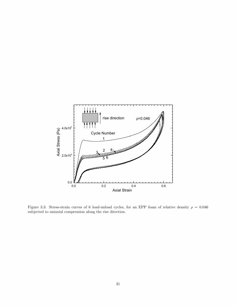
0.0 0.2 0.4 0.60.0

2.0x104

4.0x104

Axi

al S

tress

(Pa)

Axial Strain

Cycle Number1

2

rise direction

36

4

5

ρ=0.046

Figure 3.3: Stress-strain curves of 6 load-unload cycles, for an EPP foam of relative density ρ = 0.046subjected to uniaxial compression along the rise direction.

31

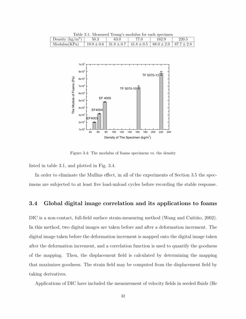
Table 3.1: Measured Young’s modulus for each specimenDensity (kg/m3) 50.3 63.0 77.0 162.9 220.5Modulus(KPa) 19.9± 0.6 31.8± 0.7 41.8± 0.5 68.0± 2.0 87.7± 2.8

40 60 80 100 120 140 160 180 200 220 2401x104

2x104

3x104

4x104

5x104

6x104

7x104

8x104

9x104

1x105

TF 5070-13

TF 5070-10

EF 4005

EF4004

The

Mod

uls

of F

oam

s (P

a)

Density of The Specimen (kg/m3)

EF4003

Figure 3.4: The modulus of foams specimens vs. the density

listed in table 3.1, and plotted in Fig. 3.4.

In order to eliminate the Mullins effect, in all of the experiments of Section 3.5 the spec-

imens are subjected to at least five load-unload cycles before recording the stable response.

3.4 Global digital image correlation and its applications to foams

DIC is a non-contact, full-field surface strain-measuring method (Wang and Cuitino, 2002).

In this method, two digital images are taken before and after a deformation increment. The

digital image taken before the deformation increment is mapped onto the digital image taken

after the deformation increment, and a correlation function is used to quantify the goodness

of the mapping. Then, the displacement field is calculated by determining the mapping

that maximizes goodness. The strain field may be computed from the displacement field by

taking derivatives.

Applications of DIC have included the measurement of velocity fields in seeded fluids (He

32

et al., 1984), the measurement of sintering shrinkage strains in powder compaction (Mizuno

et al., 1995), the characterization of surface layer cracking in soils (Cardenas-Garcia et al.,

1998), and the estimation of reliability in microelectronic packages (Lu , 1998). DIC has

been used in conjunction with advanced instrumentation systems such as scanning elec-

tron microscope (SEM) and scanning tunneling microscope (STM) for quantitative material

characterization (Lockwood et al. (1999)); Berfield et al. (2006)), and with high-speed pho-

tography for dynamic fracture studies (Chao et al., 1998). DIC has also been used for

measuring strain fields in polymeric and metallic foams (Bart-Smith et al. (1998); Zhang

et al. (1999); Bastawros et al. (2000); Wang and Cuitino (2002)). Artificial speckles are

commonly used to enhance the accuracy of the measurements, for example by imprinting a

dot map or markers using SEM electron beams (Yongqi et al., 1996) or using Fluorescent

dyes (Berfield et al., 2006), but in many cases the natural texture of the surface (of foam

specimens, for example) provides enough information (speckles) to perform the correlation.

Conventionally DIC is a local method in that it is applied over a subset of pixels (the

correlation window) of the region of interest. Thus the undeformed configuration is mapped

into the undeformed configuration over a small portion of the region of interest. To cover

the entire region of interest, DIC is applied over successive, partially overlapping correlation

windows.

Here we use the finite-element based, global DIC method first introduced by Gao et

al. (2002). In this method, a single finite-element interpolation is used to interpolate the

displacement field over the entire region of interest. Both the displacement field and the

strain field are smooth inside the finite elements and continuous across the boundaries of

the finite elements (Gao et al., 2002). The undeformed configuration is mapped onto the

undeformed configuration over the entire region of interest at once.

This global DIC method has been used is several studies, mostly involving metallic foams

(Zhou et al., 2004, 2005a,b) and soft tissues (Cao et al., 2006, 2007; Gao and Desai, 2009).

In the following sections, we perform a few calibration tests to ascertain the accuracy of our

implementation of the method.

33

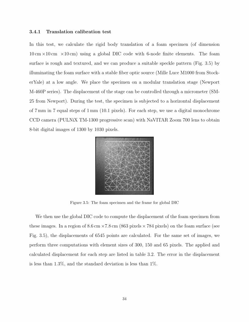
3.4.1 Translation calibration test

In this test, we calculate the rigid body translation of a foam specimen (of dimension

10 cm×10 cm ×10 cm) using a global DIC code with 6-node finite elements. The foam

surface is rough and textured, and we can produce a suitable speckle pattern (Fig. 3.5) by

illuminating the foam surface with a stable fiber optic source (Mille Luce M1000 from Stock-

erYale) at a low angle. We place the specimen on a modular translation stage (Newport

M-460P series). The displacement of the stage can be controlled through a micrometer (SM-

25 from Newport). During the test, the specimen is subjected to a horizontal displacement

of 7 mm in 7 equal steps of 1 mm (10.1 pixels). For each step, we use a digital monochrome

CCD camera (PULNiX TM-1300 progressive scan) with NaVITAR Zoom 700 lens to obtain

8-bit digital images of 1300 by 1030 pixels.

Figure 3.5: The foam specimen and the frame for global DIC

We then use the global DIC code to compute the displacement of the foam specimen from

these images. In a region of 8.6 cm×7.8 cm (863 pixels× 784 pixels) on the foam surface (see

Fig. 3.5), the displacements of 6545 points are calculated. For the same set of images, we

perform three computations with element sizes of 300, 150 and 65 pixels. The applied and

calculated displacement for each step are listed in table 3.2. The error in the displacement

is less than 1.3%, and the standard deviation is less than 1%.

34

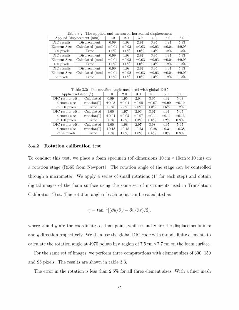
Table 3.2: The applied and measured horizontal displacementApplied Displacement (mm) 1.0 2.0 3.0 4.0 5.0 6.0

DIC results Displacement 0.99 1.98 2.97 3.95 4.94 5.93Element Size Calculated (mm) ±0.01 ±0.02 ±0.03 ±0.03 ±0.04 ±0.05

300 pixels Error 1.0% 1.0% 1.0% 1.3% 1.2% 1.2%

DIC results Displacement 0.99 1.98 2.97 3.95 4.94 5.93Element Size Calculated (mm) ±0.01 ±0.02 ±0.03 ±0.03 ±0.04 ±0.05

150 pixels Error 1.0% 1.0% 1.0% 1.3% 1.2% 1.2%

DIC results Displacement 0.99 1.98 2.97 3.95 4.94 5.93Element Size Calculated (mm) ±0.01 ±0.02 ±0.03 ±0.03 ±0.04 ±0.05

65 pixels Error 1.0% 1.0% 1.0% 1.3% 1.2% 1.2%

Table 3.3: The rotation angle measured with global DICApplied rotation (◦) 1.0 2.0 3.0 4.0 5.0 6.0

DIC results with Calculated 0.99 1.95 2.94 3.95 4.92 5.93element size rotation(◦) ±0.03 ±0.04 ±0.05 ±0.07 ±0.09 ±0.10of 300 pixels Error 1.0% 2.5% 2.0% 1.3% 1.6% 1.2%

DIC results with Calculated 1.00 1.97 2.96 3.97 4.94 5.95element size rotation(◦) ±0.04 ±0.05 ±0.07 ±0.11 ±0.11 ±0.13of 150 pixels Error 0.0% 1.5% 1.3% 0.8% 1.2% 0.8%

DIC results with Calculated 1.00 1.98 2.97 3.98 4.95 5.95element size rotation(◦) ±0.13 ±0.18 ±0.23 ±0.28 ±0.31 ±0.38of 95 pixels Error 0.0% 1.0% 1.0% 0.5% 1.0% 0.8%

3.4.2 Rotation calibration test

To conduct this test, we place a foam specimen (of dimensions 10 cm× 10cm× 10 cm) on

a rotation stage (RS65 from Newport). The rotation angle of the stage can be controlled

through a micrometer. We apply a series of small rotations (1◦ for each step) and obtain

digital images of the foam surface using the same set of instruments used in Translation

Calibration Test. The rotation angle of each point can be calculated as

γ = tan−1[(∂u/∂y − ∂v/∂x)/2],

where x and y are the coordinates of that point, while u and v are the displacements in x

and y direction respectively. We then use the global DIC code with 6-node finite elements to

calculate the rotation angle at 4970 points in a region of 7.5 cm×7.7 cm on the foam surface.

For the same set of images, we perform three computations with element sizes of 300, 150

and 95 pixels. The results are shown in table 3.3.

The error in the rotation is less than 2.5% for all three element sizes. With a finer mesh

35

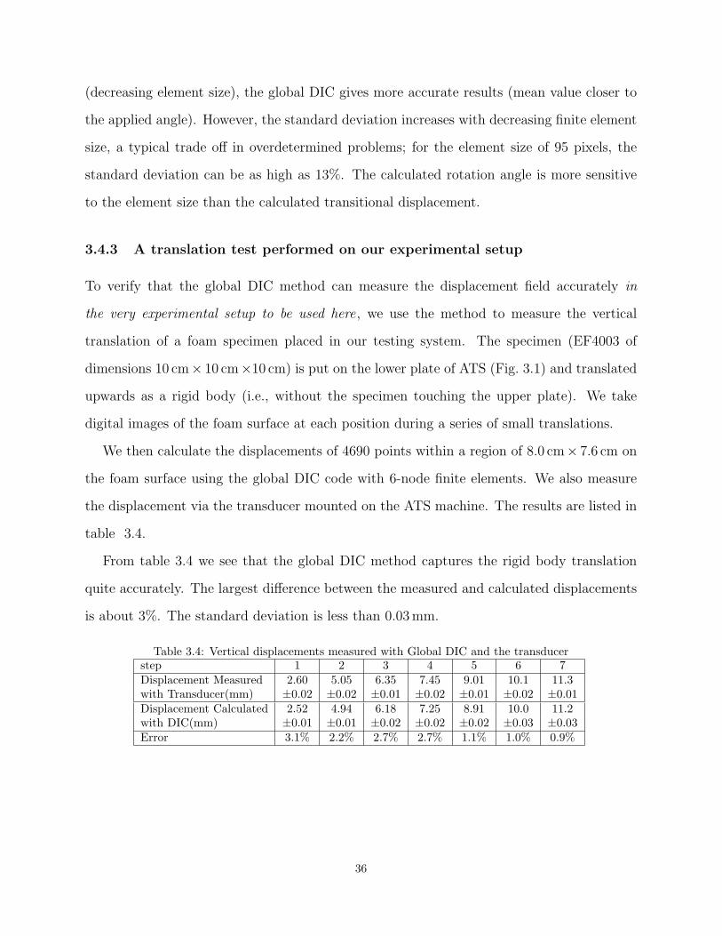
(decreasing element size), the global DIC gives more accurate results (mean value closer to

the applied angle). However, the standard deviation increases with decreasing finite element

size, a typical trade off in overdetermined problems; for the element size of 95 pixels, the

standard deviation can be as high as 13%. The calculated rotation angle is more sensitive

to the element size than the calculated transitional displacement.

3.4.3 A translation test performed on our experimental setup

To verify that the global DIC method can measure the displacement field accurately in

the very experimental setup to be used here, we use the method to measure the vertical

translation of a foam specimen placed in our testing system. The specimen (EF4003 of

dimensions 10 cm× 10 cm×10 cm) is put on the lower plate of ATS (Fig. 3.1) and translated

upwards as a rigid body (i.e., without the specimen touching the upper plate). We take

digital images of the foam surface at each position during a series of small translations.

We then calculate the displacements of 4690 points within a region of 8.0 cm× 7.6 cm on

the foam surface using the global DIC code with 6-node finite elements. We also measure

the displacement via the transducer mounted on the ATS machine. The results are listed in

table 3.4.

From table 3.4 we see that the global DIC method captures the rigid body translation

quite accurately. The largest difference between the measured and calculated displacements

is about 3%. The standard deviation is less than 0.03 mm.

Table 3.4: Vertical displacements measured with Global DIC and the transducerstep 1 2 3 4 5 6 7Displacement Measured 2.60 5.05 6.35 7.45 9.01 10.1 11.3with Transducer(mm) ±0.02 ±0.02 ±0.01 ±0.02 ±0.01 ±0.02 ±0.01Displacement Calculated 2.52 4.94 6.18 7.25 8.91 10.0 11.2with DIC(mm) ±0.01 ±0.01 ±0.02 ±0.02 ±0.02 ±0.03 ±0.03Error 3.1% 2.2% 2.7% 2.7% 1.1% 1.0% 0.9%

36

3.5 Experimental results

In order to eliminate the Mullins effect, in all of the experiments that follow the specimens

are subjected to at least five load-unload cycles before recording the stable response (see

Section 3.3 above).

All the DIC computations are performed using the global DIC code with 6-node finite

elements of Section 3.4.

The estimated relative error of the stress and strain values reported here is about 5% (see

Section 3.2.1 above).

3.5.1 Uniaxial compression along the rise direction

To prevent bulging (see Section 3.6 below), we use foam specimens of dimensions 5.0 cm×10.0 cm× 10.0 cm. The height of 5.0 cm is along the rise direction.

We define the axial stress as the loading force divided by the original normal cross section

area and the axial strain as the change of height divided by the original height of the

specimen. We verify that the foam specimens are not strain-rate sensitive (Gioia et al.,

2001), and use a constant loading rate of 0.3 cm/min for all the 5 foam specimens, which

translates to a strain rate of 1 × 10−3 /s. The axial stress vs. axial strain curves are shown

in Fig. 3.6.

The results clearly show a difference in the stress-strain response of low-density and high-

density foams. For low-density foams (ρ = 0.030, 0.038, 0.046), three distinct regions of the

response can be identified. For small strains ( ≤ 5%), the stress-strain response is almost

linear. This is followed by an extended stress plateau wherein the stress remains constant

for increasing values of axial strain. For the lowest density specimen, the plateau is seen

to extend up to almost 25% axial strain. Where the stress plateau ends, we recover a

monotonically increasing stress-strain response and the stress starts to increase rapidly with

increasing values of applied strain. The width of the stress plateau lessens with increasing

density. For the high-density foams (ρ = 0.065, 0.086) no plateau is observed, and the stress

37

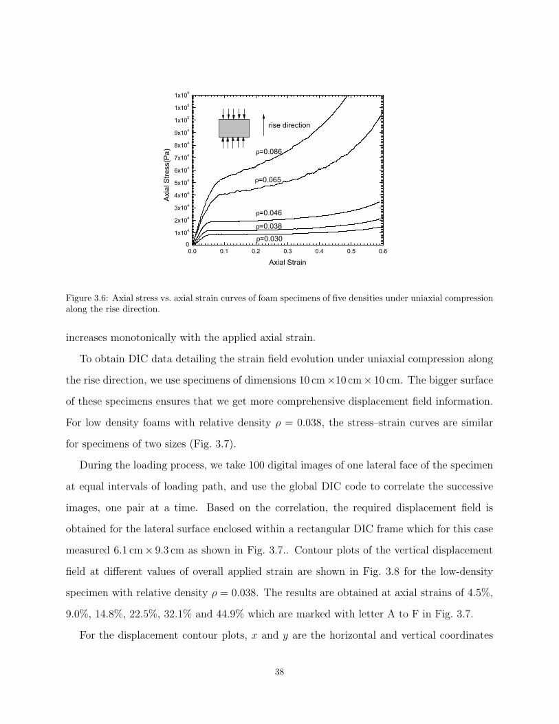
0.0 0.1 0.2 0.3 0.4 0.5 0.60

1x104

2x104

3x104

4x104

5x104

6x104

7x104

8x104

9x104

1x105

1x105

1x105

ρ=0.030

ρ=0.038

ρ=0.046

ρ=0.065

Axi

al S

tress

(Pa)

Axial Strain

ρ=0.086

rise direction

Figure 3.6: Axial stress vs. axial strain curves of foam specimens of five densities under uniaxial compressionalong the rise direction.

increases monotonically with the applied axial strain.

To obtain DIC data detailing the strain field evolution under uniaxial compression along

the rise direction, we use specimens of dimensions 10 cm×10 cm× 10 cm. The bigger surface

of these specimens ensures that we get more comprehensive displacement field information.

For low density foams with relative density ρ = 0.038, the stress–strain curves are similar

for specimens of two sizes (Fig. 3.7).

During the loading process, we take 100 digital images of one lateral face of the specimen

at equal intervals of loading path, and use the global DIC code to correlate the successive

images, one pair at a time. Based on the correlation, the required displacement field is

obtained for the lateral surface enclosed within a rectangular DIC frame which for this case

measured 6.1 cm× 9.3 cm as shown in Fig. 3.7.. Contour plots of the vertical displacement

field at different values of overall applied strain are shown in Fig. 3.8 for the low-density

specimen with relative density ρ = 0.038. The results are obtained at axial strains of 4.5%,

9.0%, 14.8%, 22.5%, 32.1% and 44.9% which are marked with letter A to F in Fig. 3.7.

For the displacement contour plots, x and y are the horizontal and vertical coordinates

38

0.0 0.1 0.2 0.3 0.4 0.5 0.6 0.70

1x104

2x104

3x104

4x104

10x10x10 specimen 10x10x5 specimen

Axi

al S

tress

(Pa)

Axial Strain

=0.038

rise direction

A B C D EF

DIC Frame

Figure 3.7: Axial stress vs. axial strain curve of the low density foam specimen under uniaxial compressionalong the rise direction.

of the image of the undeformed specimen face with a scale of 1 pixel = 0.1 mm. The lines

within the image are contours of equal displacement plotted at increments of 0.77 mm. The

minimum and maximum displacement in each plot is marked. The spacing between the

contours gives an indication of the strain distribution in the specimen.

At low strains ( pt. A) the contours are equidistant, indicating a homogeneous strain

distribution through the sample. For strains that lie within the stress plateau (pt. B, C and

D), the strain field shows a heterogeneous distribution with two preferred values of strain

coexisting in the specimen. A high strain zone is seen near the center of the specimen and

is bounded by two regions of relatively low strain. As the deformation proceeds, we see the

volume fraction of the high strain zone growing at the expense of the volume fraction of the

low strain zone. As the entire specimen switches to a high strain configuration, we recover a

homogeneous field at pt. E, and the field remains homogeneous under further deformation.

To show the trend more clearly, we plot the displacement in y direction along a line on

the foam surface (the dashed line shown in Fig. 3.8a). The results are shown in Fig. 3.9,

For low and high values of applied strain (corresponding to pts. A and F on the stress-strain

curve of Fig. 3.7), that the slopes (displacement/position) are uniform (straight lines in

39

x (pixels)

y(p

ixel

s)

400 600 800

200

400

600

8004.1 mm

1.0 mm

(a)

x (pixels)

y(p

ixel

s)

400 600 800

200

400

600

800

7.9 mm

1.0 mm

(b)

x (pixels)

y(p

ixel

s)

400 600 800

200

400

600

800

13.3 mm

1.8 mm

(c)

x (pixels)

y(p

ixel

s)

400 600 800

200

400

600

800

20.9 mm

1.8 mm

(d)

x (pixels)

y(p

ixel

s)

400 600 800

200

400

600

800

30.9 mm

2.6 mm

(e)

x (pixels)

y(p

ixel

s)

400 600 800

200

400

600

800

43.9 mm

2.6 mm

(f)

Figure 3.8: Contours of displacement along the rise direction for the foam of lower density.

40

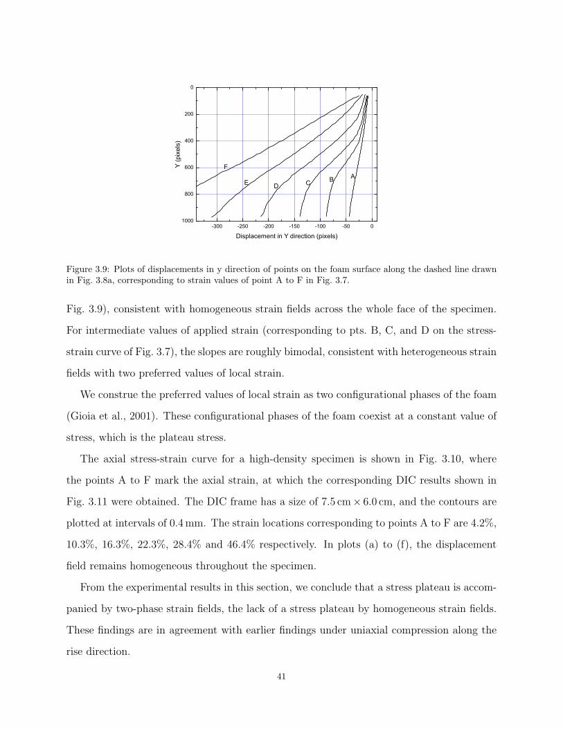
-300 -250 -200 -150 -100 -50 01000

800

600

400

200

0

D

F

E

Y (p

ixel

s)

Displacement in Y direction (pixels)

ABC

Figure 3.9: Plots of displacements in y direction of points on the foam surface along the dashed line drawnin Fig. 3.8a, corresponding to strain values of point A to F in Fig. 3.7.

Fig. 3.9), consistent with homogeneous strain fields across the whole face of the specimen.

For intermediate values of applied strain (corresponding to pts. B, C, and D on the stress-

strain curve of Fig. 3.7), the slopes are roughly bimodal, consistent with heterogeneous strain

fields with two preferred values of local strain.

We construe the preferred values of local strain as two configurational phases of the foam

(Gioia et al., 2001). These configurational phases of the foam coexist at a constant value of

stress, which is the plateau stress.

The axial stress-strain curve for a high-density specimen is shown in Fig. 3.10, where

the points A to F mark the axial strain, at which the corresponding DIC results shown in

Fig. 3.11 were obtained. The DIC frame has a size of 7.5 cm× 6.0 cm, and the contours are

plotted at intervals of 0.4 mm. The strain locations corresponding to points A to F are 4.2%,

10.3%, 16.3%, 22.3%, 28.4% and 46.4% respectively. In plots (a) to (f), the displacement

field remains homogeneous throughout the specimen.

From the experimental results in this section, we conclude that a stress plateau is accom-

panied by two-phase strain fields, the lack of a stress plateau by homogeneous strain fields.

These findings are in agreement with earlier findings under uniaxial compression along the

rise direction.

41

0.0 0.1 0.2 0.3 0.4 0.5 0.6 0.70.0

2.0x104

4.0x104

6.0x104

8.0x104

1.0x105

1.2x105

10x10x10 Specimen 10x10x5 Specimen

Axi

al S

tress

(Pa)

Axial Strain

=0.064

rise direction

A

B C D E

F

DIC Frame

Figure 3.10: Axial stress vs. axial strain curve of the high density foam specimen under uniaxial compressionalong the rise direction.

y(p

ixel

s)

400 600 800

300

400

500

600

700

1.6 mm

3.6 mm

x (pixels)

(a)

y(p

ixel

s)

400 600 800

300

400

500

600

700

2.8 mm

8.0 mm

x (pixels)

(b)

y(p

ixel

s)

400 600 800

300

400

500

600

700

3.6 mm

12.7 mm

x (pixels)

(c)

y(p

ixel

s)

400 600 800

300

400

500

600

700

4.4 mm

17.5 mmx (pixels)

(d)

y(p

ixel

s)

400 600 800

300

400

500

600

700

6.4 mm

21.9 mmx (pixels)

(e)

y(p

ixel

s)

400 600 800

300

400

500

600

700

10.0 mm

36.3 mmx (pixels)

(f)

Figure 3.11: Contours of displacement along the rise direction for the foam of higher density under uniaxialcompression along the rise direction.

42

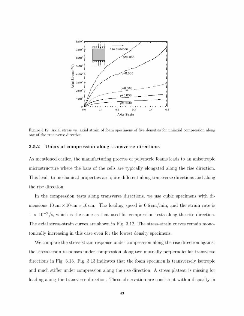
0.0 0.1 0.2 0.3 0.4 0.50

1x104

2x104

3x104

4x104

5x104

6x104

7x104

8x104

ρ=0.030

ρ=0.038

ρ=0.046

ρ=0.065

Axi

al S

tress

(Pa)

Axial Strain

ρ=0.086

rise direction

Figure 3.12: Axial stress vs. axial strain of foam specimens of five densities for uniaxial compression alongone of the transverse direction

3.5.2 Uniaxial compression along transverse directions

As mentioned earlier, the manufacturing process of polymeric foams leads to an anisotropic

microstructure where the bars of the cells are typically elongated along the rise direction.

This leads to mechanical properties are quite different along transverse directions and along

the rise direction.

In the compression tests along transverse directions, we use cubic specimens with di-

mensions 10 cm× 10 cm× 10 cm. The loading speed is 0.6 cm/min, and the strain rate is

1 × 10−3 /s, which is the same as that used for compression tests along the rise direction.

The axial stress-strain curves are shown in Fig. 3.12. The stress-strain curves remain mono-

tonically increasing in this case even for the lowest density specimens.

We compare the stress-strain response under compression along the rise direction against

the stress-strain responses under compression along two mutually perperndicular transverse

directions in Fig. 3.13. Fig. 3.13 indicates that the foam specimen is transversely isotropic

and much stiffer under compression along the rise direction. A stress plateau is missing for

loading along the transverse direction. These observation are consistent with a disparity in

43

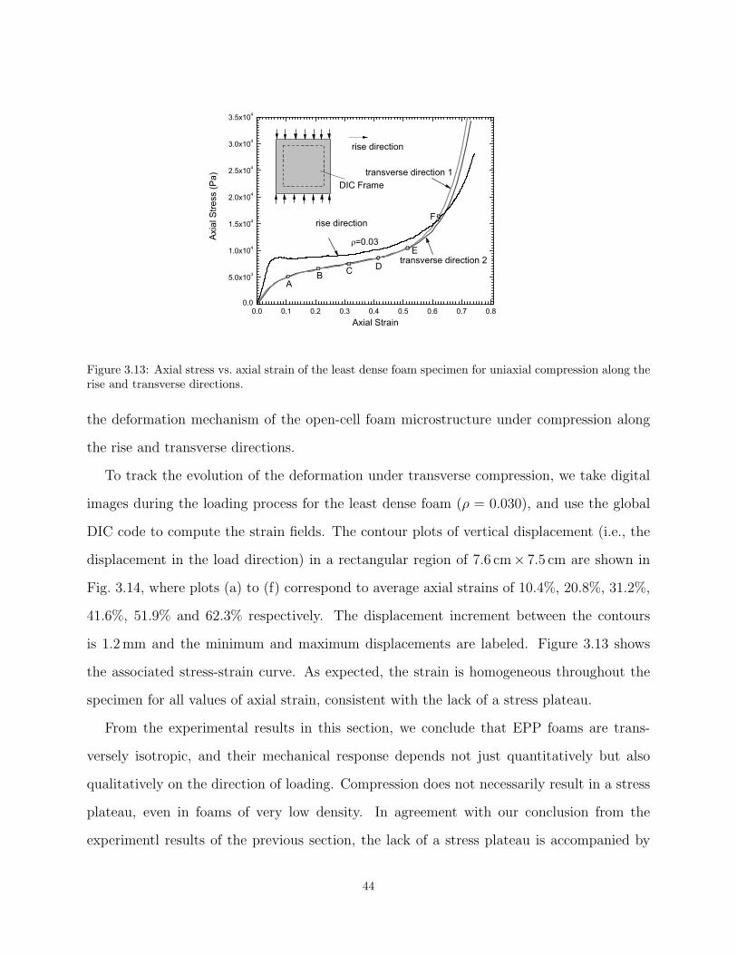
0.0 0.1 0.2 0.3 0.4 0.5 0.6 0.7 0.80.0

5.0x103

1.0x104

1.5x104

2.0x104

2.5x104

3.0x104

3.5x104

F

E

DC

Axi

al S

tress

(Pa)

Axial Strain

=0.03

rise direction

transverse direction 1

transverse direction 2

AB

DIC Frame

rise direction

Figure 3.13: Axial stress vs. axial strain of the least dense foam specimen for uniaxial compression along therise and transverse directions.

the deformation mechanism of the open-cell foam microstructure under compression along

the rise and transverse directions.

To track the evolution of the deformation under transverse compression, we take digital

images during the loading process for the least dense foam (ρ = 0.030), and use the global

DIC code to compute the strain fields. The contour plots of vertical displacement (i.e., the

displacement in the load direction) in a rectangular region of 7.6 cm× 7.5 cm are shown in

Fig. 3.14, where plots (a) to (f) correspond to average axial strains of 10.4%, 20.8%, 31.2%,

41.6%, 51.9% and 62.3% respectively. The displacement increment between the contours

is 1.2 mm and the minimum and maximum displacements are labeled. Figure 3.13 shows

the associated stress-strain curve. As expected, the strain is homogeneous throughout the

specimen for all values of axial strain, consistent with the lack of a stress plateau.

From the experimental results in this section, we conclude that EPP foams are trans-

versely isotropic, and their mechanical response depends not just quantitatively but also

qualitatively on the direction of loading. Compression does not necessarily result in a stress

plateau, even in foams of very low density. In agreement with our conclusion from the

experimentl results of the previous section, the lack of a stress plateau is accompanied by

44

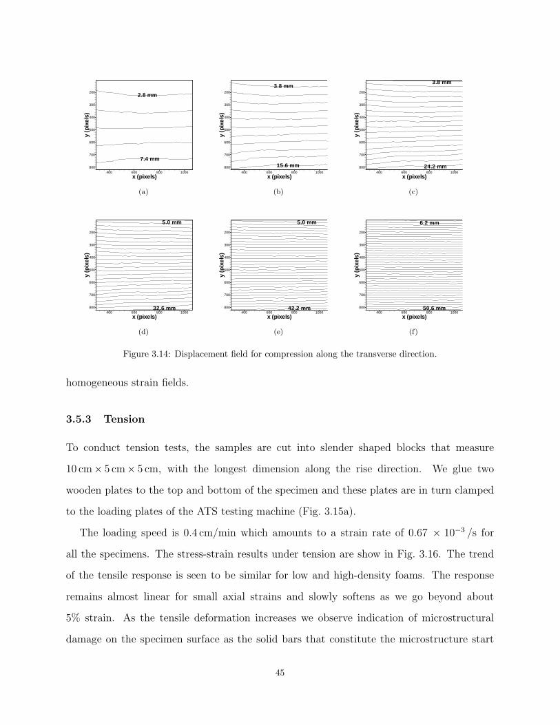
x (pixels)

y(p

ixel

s)

400 600 800 1000

200

300

400

500

600

700

800

7.4 mm

2.8 mm

(a)

x (pixels)

y(p

ixel

s)

400 600 800 1000

200

300

400

500

600

700

800 15.6 mm

3.8 mm

(b)

x (pixels)

y(p

ixel

s)

400 600 800 1000

200

300

400

500

600

700

800 24.2 mm

3.8 mm

(c)

x (pixels)

y(p

ixel

s)

400 600 800 1000

200

300

400

500

600

700

800 32.6 mm

5.0 mm

(d)

x (pixels)

y(p

ixel

s)

400 600 800 1000

200

300

400

500

600

700

800 42.2 mm

5.0 mm

(e)

x (pixels)

y(p

ixel

s)

400 600 800 1000

200

300

400

500

600

700

800 50.6 mm

6.2 mm

(f)

Figure 3.14: Displacement field for compression along the transverse direction.

homogeneous strain fields.

3.5.3 Tension

To conduct tension tests, the samples are cut into slender shaped blocks that measure

10 cm× 5 cm× 5 cm, with the longest dimension along the rise direction. We glue two

wooden plates to the top and bottom of the specimen and these plates are in turn clamped

to the loading plates of the ATS testing machine (Fig. 3.15a).

The loading speed is 0.4 cm/min which amounts to a strain rate of 0.67 × 10−3 /s for

all the specimens. The stress-strain results under tension are show in Fig. 3.16. The trend

of the tensile response is seen to be similar for low and high-density foams. The response

remains almost linear for small axial strains and slowly softens as we go beyond about

5% strain. As the tensile deformation increases we observe indication of microstructural

damage on the specimen surface as the solid bars that constitute the microstructure start

45

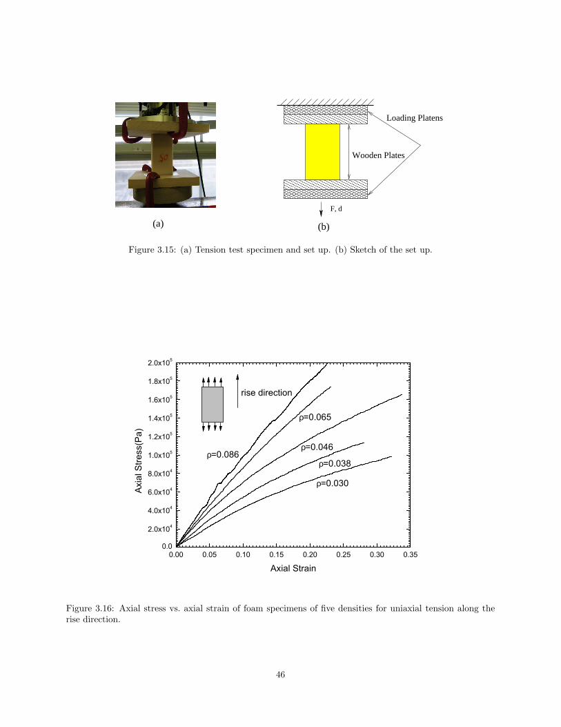
F, d

������������������������������������

���������������������������

���������������������������������������������������������������

���������������������������

���������������������������

(a) (b)

Wooden Plates

Loading Platens

Figure 3.15: (a) Tension test specimen and set up. (b) Sketch of the set up.

0.00 0.05 0.10 0.15 0.20 0.25 0.30 0.350.0

2.0x104

4.0x104

6.0x104

8.0x104

1.0x105

1.2x105

1.4x105

1.6x105

1.8x105

2.0x105

ρ=0.030

ρ=0.038

ρ=0.046

ρ=0.065

Axi

al S

tress

(Pa)

Axial Strain

ρ=0.086

rise direction

Figure 3.16: Axial stress vs. axial strain of foam specimens of five densities for uniaxial tension along therise direction.

46

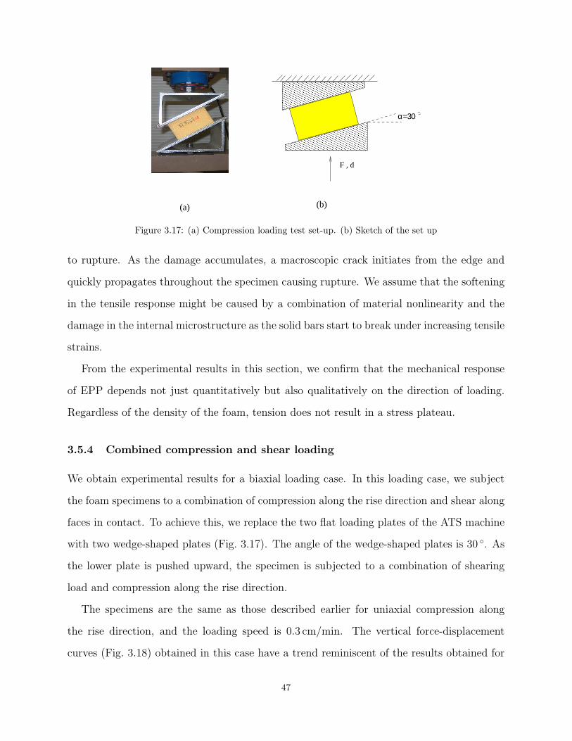
(b)

�����������������������������������������������������������������������������

�����������������������������������������������������������������������������

�����������������������������������������������������������������������������

�����������������������������������������������������������������������������

F , d

α=30

(a)

Figure 3.17: (a) Compression loading test set-up. (b) Sketch of the set up

to rupture. As the damage accumulates, a macroscopic crack initiates from the edge and

quickly propagates throughout the specimen causing rupture. We assume that the softening

in the tensile response might be caused by a combination of material nonlinearity and the

damage in the internal microstructure as the solid bars start to break under increasing tensile

strains.

From the experimental results in this section, we confirm that the mechanical response

of EPP depends not just quantitatively but also qualitatively on the direction of loading.

Regardless of the density of the foam, tension does not result in a stress plateau.

3.5.4 Combined compression and shear loading

We obtain experimental results for a biaxial loading case. In this loading case, we subject

the foam specimens to a combination of compression along the rise direction and shear along

faces in contact. To achieve this, we replace the two flat loading plates of the ATS machine

with two wedge-shaped plates (Fig. 3.17). The angle of the wedge-shaped plates is 30 ◦. As

the lower plate is pushed upward, the specimen is subjected to a combination of shearing

load and compression along the rise direction.

The specimens are the same as those described earlier for uniaxial compression along

the rise direction, and the loading speed is 0.3 cm/min. The vertical force-displacement

curves (Fig. 3.18) obtained in this case have a trend reminiscent of the results obtained for

47

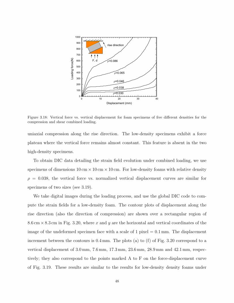
0 10 20 30 400

100

200

300

400

500

600

700

800

900

1000

=0.030

=0.038

=0.046

=0.065

Load

ing

forc

e(N

)

Displacement (mm)

=0.086F, d

rise direction

Figure 3.18: Vertical force vs. vertical displacement for foam specimens of five different densities for thecompression and shear combined loading.

uniaxial compression along the rise direction. The low-density specimens exhibit a force

plateau where the vertical force remains almost constant. This feature is absent in the two

high-density specimens.

To obtain DIC data detailing the strain field evolution under combined loading, we use

specimens of dimensions 10 cm× 10 cm× 10 cm. For low-density foams with relative density

ρ = 0.038, the vertical force vs. normalized vertical displacement curves are similar for

specimens of two sizes (see 3.19).

We take digital images during the loading process, and use the global DIC code to com-

pute the strain fields for a low-density foam. The contour plots of displacement along the

rise direction (also the direction of compression) are shown over a rectangular region of

8.6 cm× 8.3 cm in Fig. 3.20, where x and y are the horizontal and vertical coordinates of the

image of the undeformed specimen face with a scale of 1 pixel = 0.1 mm. The displacement

increment between the contours is 0.4 mm. The plots (a) to (f) of Fig. 3.20 correspond to a

vertical displacement of 3.0 mm, 7.6 mm, 17.3 mm, 23.6 mm, 28.9 mm and 42.1 mm, respec-

tively; they also correspond to the points marked A to F on the force-displacement curve

of Fig. 3.19. These results are similar to the results for low-density density foams under

48

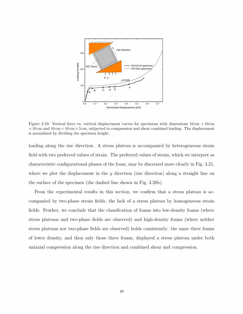
0.0 0.1 0.2 0.3 0.4 0.5 0.6 0.70

100

200

300

10x10x10 specimen 10x10x5 specimen

=0.038

Load

ing

forc

e(N

)

Nomorlized Displacement (d/H)

F, d

rise direction

DIC frame

AB C D E

F

Figure 3.19: Vertical force vs. vertical displacement curves for specimens with dimensions 10 cm × 10 cm× 10 cm and 10 cm× 10 cm× 5 cm, subjected to compression and shear combined loading. The displacementis normalized by dividing the specimen height.

loading along the rise direction. A stress plateau is accompanied by heterogeneous strain

field with two preferred values of strain. The preferred values of strain, which we interpret as

characteristic configurational phases of the foam, may be discerned more clearly in Fig. 3.21,

where we plot the displacement in the y direction (rise direction) along a straight line on

the surface of the specimen (the dashed line shown in Fig. 3.20b).

From the experimental results in this section, we confirm that a stress plateau is ac-

companied by two-phase strain fields, the lack of a stress plateau by homogeneous strain

fields. Fruther, we conclude that the classification of foams into low-density foams (where

stress plateaus and two-phase fields are observed) and high-density foams (where neither

stress plateaus nor two-phase fields are observed) holds consistently: the same three foams

of lower density, and then only those three foams, displayed a stress plateau under both

uniaxial compression along the rise direction and combined shear and compression.

49

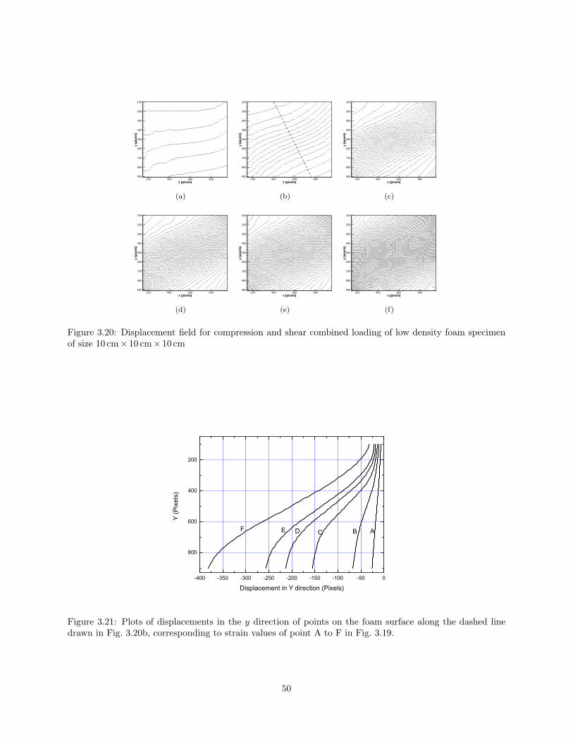
x (pixels)

y(p

ixel

s)

200 400 600 800

100

200

300

400

500

600

700

800

900

(a)

x (pixels)

y(p

ixel

s)

200 400 600 800

100

200

300

400

500

600

700

800

900

(b)

x (pixels)

y(p

ixel

s)

200 400 600 800

100

200

300

400

500

600

700

800

900

(c)

x (pixels)

y(p

ixel

s)

200 400 600 800

100

200

300

400

500

600

700

800

900

(d)

x (pixels)

y(p

ixel

s)

200 400 600 800

100

200

300

400

500

600

700

800

900

(e)

x (pixels)

y(p

ixel

s)

200 400 600 800

100

200

300

400

500

600

700

800

900

(f)

Figure 3.20: Displacement field for compression and shear combined loading of low density foam specimenof size 10 cm× 10 cm× 10 cm

-400 -350 -300 -250 -200 -150 -100 -50 0

800

600

400

200

Y (P

ixel

s)

Displacement in Y direction (Pixels)

ABCDEF

Figure 3.21: Plots of displacements in the y direction of points on the foam surface along the dashed linedrawn in Fig. 3.20b, corresponding to strain values of point A to F in Fig. 3.19.

50

0.0 0.1 0.2 0.3 0.4 0.50

5000

10000

15000

20000

25000

30000

0.0 0.1 0.2 0.3 0.4 0.50

2000

4000

6000

8000

10000

12000

14000

16000

0.0 0.1 0.2 0.3 0.4 0.50

20000

40000

60000

80000

100000

0.0 0.1 0.2 0.3 0.4 0.50

20000

40000

60000

80000

100000

120000

140000

8.07KPa

=0.065

=0.046

Axi

al S

tress

(Pa)

Axial Strain

(b)

2.07KPa

4.55KPa

Axi

al S

tress

(Pa)

Axial Strain

(a)

=0.038

2.21KPa

3.10KPa

5.10KPa

Axi

al S

tress

(Pa)

Axial Strain

(c)

10.3KPa

24.1KPa

41.3KPa

=0.086

Axi

al S

tress

(Pa)

Axial Strain

(d)

10.3KPa

27.6KPa

51.0KPa

Figure 3.22: Vertical force vs. vertical displacement curves for triaxial loading

51

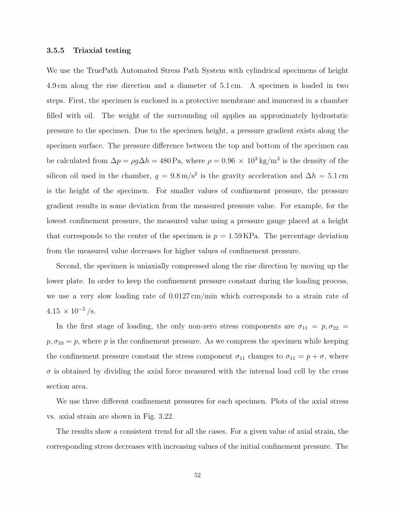
3.5.5 Triaxial testing

We use the TruePath Automated Stress Path System with cylindrical specimens of height

4.9 cm along the rise direction and a diameter of 5.1 cm. A specimen is loaded in two

steps. First, the specimen is enclosed in a protective membrane and immersed in a chamber

filled with oil. The weight of the surrounding oil applies an approximately hydrostatic

pressure to the specimen. Due to the specimen height, a pressure gradient exists along the

specimen surface. The pressure difference between the top and bottom of the specimen can

be calculated from ∆p = ρg∆h = 480 Pa, where ρ = 0.96 × 103 kg/m3 is the density of the

silicon oil used in the chamber, g = 9.8 m/s2 is the gravity acceleration and ∆h = 5.1 cm

is the height of the specimen. For smaller values of confinement pressure, the pressure

gradient results in some deviation from the measured pressure value. For example, for the

lowest confinement pressure, the measured value using a pressure gauge placed at a height

that corresponds to the center of the specimen is p = 1.59 KPa. The percentage deviation

from the measured value decreases for higher values of confinement pressure.

Second, the specimen is uniaxially compressed along the rise direction by moving up the

lower plate. In order to keep the confinement pressure constant during the loading process,

we use a very slow loading rate of 0.0127 cm/min which corresponds to a strain rate of

4.15 × 10−5 /s.

In the first stage of loading, the only non-zero stress components are σ11 = p, σ22 =

p, σ33 = p, where p is the confinement pressure. As we compress the specimen while keeping

the confinement pressure constant the stress component σ11 changes to σ11 = p + σ, where

σ is obtained by dividing the axial force measured with the internal load cell by the cross

section area.

We use three different confinement pressures for each specimen. Plots of the axial stress

vs. axial strain are shown in Fig. 3.22.

The results show a consistent trend for all the cases. For a given value of axial strain, the

corresponding stress decreases with increasing values of the initial confinement pressure. The

52

initial confinement pressure leads to a softer response. Very high values of initial confinement

pressure seem to change the stress-strain response (curves in gray in Fig. 3.22A, D, and E

which correspond to a confinement pressure of 57.9 KPa, 41.3 KPa and 51.0 KPa for for

specimens of relative density ρ = 0.030, ρ = 0.065 and ρ = 0.086 respectively).

3.6 The bulging of foam specimens elucidated via the global

DIC method

During uniaxial compression tests we have observed a frequent phenomenon of bulging ,

whereby the specimen starts to bend and eventually forms a sharp cusp on one side. The

phenomenon occurs only in low-density EPP foams, and only where the compression is along

the rise direction For foam specimens of higher densities, there is no bulging.

An example of bulging is shown in Fig. 3.23, where a cubic foam specimen is compressed

with a constant loading rate of 0.1 mm/sec (or strain rate of 1 × 10−3/sec) on the ATS

testing machine.

To study the bulging in some detail, we use global DIC to calculate the displacement

field of a region of size 7.7 cm× 8.2 cm on the surface the foam specimen. During loading,

we take a series of digital images of the foam surface. Between any two consecutive images,

the time interval is 5 seconds, and the displacement of the loading plate is 0.5 mm. We take

a total of 140 images.

We then use the global DIC code with 6-node finite elements to compute the displacement

field. The finite element size is 130 pixels (about 1.3 cm on the foam surface). The foam

specimen and the finite element mesh are shown in Fig. 3.24.

We calculate the displacement field of all 140 steps. A few of the deformed finite element

meshes are shown in Fig. 3.25.

The contours of the displacement along the loading direction (vertical direction of Fig. 3.24)

are shown in Fig. 3.26, where the displacement contours of (a) to (f) are drawn on the

undeformed configuration (Lagrangian coordinates) and correspond to the deformation of

53

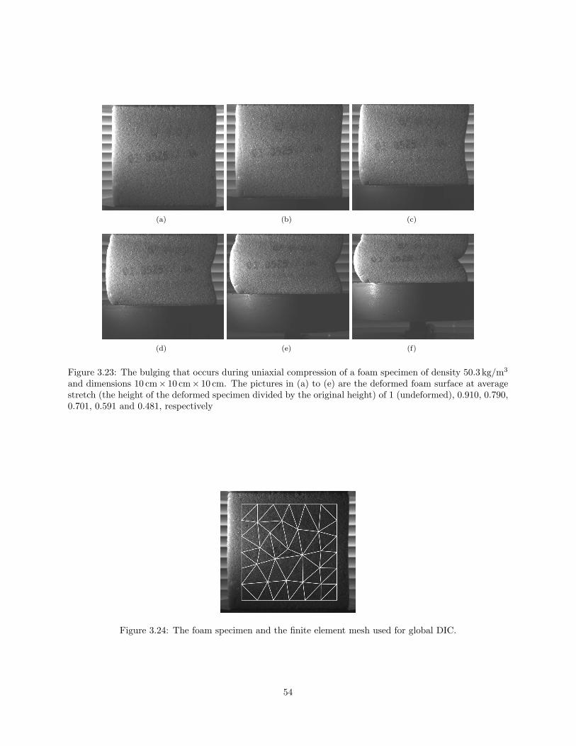
(a) (b) (c)

(d) (e) (f)

Figure 3.23: The bulging that occurs during uniaxial compression of a foam specimen of density 50.3 kg/m3

and dimensions 10 cm× 10 cm× 10 cm. The pictures in (a) to (e) are the deformed foam surface at averagestretch (the height of the deformed specimen divided by the original height) of 1 (undeformed), 0.910, 0.790,0.701, 0.591 and 0.481, respectively

Figure 3.24: The foam specimen and the finite element mesh used for global DIC.

54

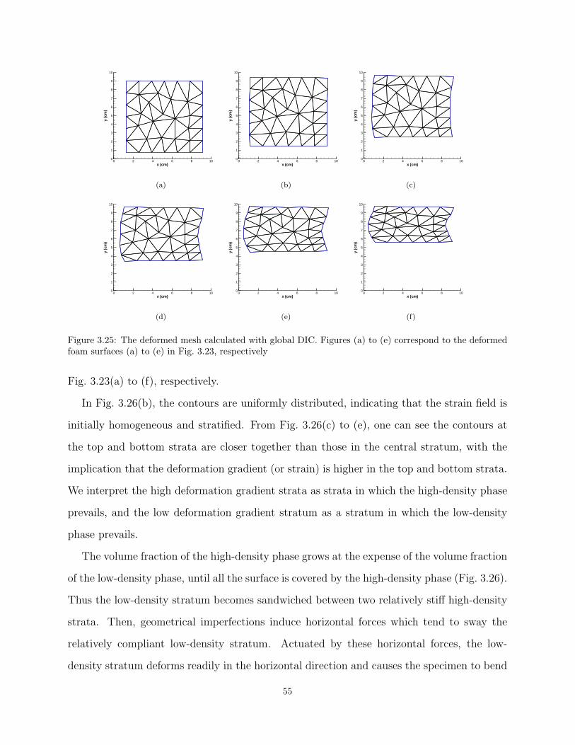
x (cm)

y(c

m)

0 2 4 6 8 100

1

2

3

4

5

6

7

8

9

10

(a)

x (cm)

y(c

m)

0 2 4 6 8 100

1

2

3

4

5

6

7

8

9

10

(b)

x (cm)

y(c

m)

0 2 4 6 8 100

1

2

3

4

5

6

7

8

9

10

(c)

x (cm)

y(c

m)

0 2 4 6 8 100

1

2

3

4

5

6

7

8

9

10

(d)

x (cm)

y(c

m)

0 2 4 6 8 100

1

2

3

4

5

6

7

8

9

10

(e)

x (cm)

y(c

m)

0 2 4 6 8 100

1

2

3

4

5

6

7

8

9

10

(f)

Figure 3.25: The deformed mesh calculated with global DIC. Figures (a) to (e) correspond to the deformedfoam surfaces (a) to (e) in Fig. 3.23, respectively

Fig. 3.23(a) to (f), respectively.

In Fig. 3.26(b), the contours are uniformly distributed, indicating that the strain field is

initially homogeneous and stratified. From Fig. 3.26(c) to (e), one can see the contours at

the top and bottom strata are closer together than those in the central stratum, with the

implication that the deformation gradient (or strain) is higher in the top and bottom strata.

We interpret the high deformation gradient strata as strata in which the high-density phase

prevails, and the low deformation gradient stratum as a stratum in which the low-density

phase prevails.

The volume fraction of the high-density phase grows at the expense of the volume fraction

of the low-density phase, until all the surface is covered by the high-density phase (Fig. 3.26).

Thus the low-density stratum becomes sandwiched between two relatively stiff high-density

strata. Then, geometrical imperfections induce horizontal forces which tend to sway the

relatively compliant low-density stratum. Actuated by these horizontal forces, the low-

density stratum deforms readily in the horizontal direction and causes the specimen to bend

55

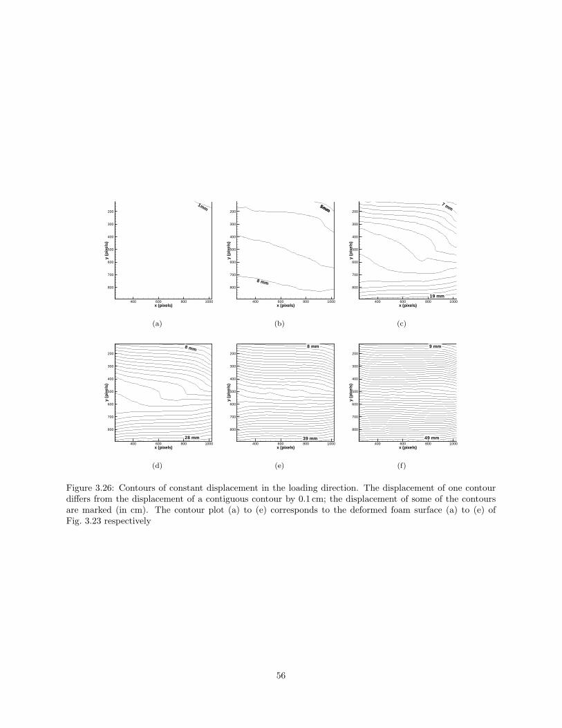
x (pixels)

y(p

ixel

s)

400 600 800 1000

200

300

400

500

600

700

800

1mm

(a)

x (pixels)

y(p

ixel

s)

400 600 800 1000

200

300

400

500

600

700

800

5mm5mm

8 mm

(b)

x (pixels)

y(p

ixel

s)

400 600 800 1000

200

300

400

500

600

700

800

7 mm

19 mm

(c)

x (pixels)

y(p

ixel

s)

400 600 800 1000

200

300

400

500

600

700

800

8 mm

28 mm

(d)

x (pixels)

y(p

ixel

s)

400 600 800 1000

200

300

400

500

600

700

800

8 mm

39 mm

(e)

x (pixels)

y(p

ixel

s)

400 600 800 1000

200

300

400

500

600

700

800

9 mm

49 mm

(f)

Figure 3.26: Contours of constant displacement in the loading direction. The displacement of one contourdiffers from the displacement of a contiguous contour by 0.1 cm; the displacement of some of the contoursare marked (in cm). The contour plot (a) to (e) corresponds to the deformed foam surface (a) to (e) ofFig. 3.23 respectively

56

and eventually to form a cusp on one side af the speciment, and a bulge on the other side.

We conclude that bulging is closely associated with the occurrence of a phase transition;

to avoid bulging where the direction of loading coincides with the rise direction, one must

use specimens that are relatively short in the rise direction (as we have done in Section 3.5).

In this example, the global DIC code with 6-node finite elements is able to capture the

very large (up to compression strain of 70%) nonuniform deformation of the bulging foam

specimen. It also affords insight into the mechanism of bulging and the formation of cusps

in low-density foams.

3.7 Discussion

Four observations about the current state of research on elastic polyether polyurethane

(EPP) foams have guided us in designing the experiments of this chapter.

1. Most practical applications of EPP foams involve multiaxial loading, yet there has

been scant research on the mechanical response of EPP foams under multiaxial states

of stress.

2. The mechanical response of an EPP foam depends not just quantitatively but qualita-

tively on the relative density of the foam, yet no experiments have been reported for a

set of EPP foams of widely differing densities.

3. EPP foams are commonly subjected to large strains under service conditions, yet mea-

surements of complete stress-strain curves have remained scarce and mostly limited to

uniaxial tests.

4. A stress plateau appears to be invariably accompanied by heterogeneous strain fields,

yet measurements of the strain fields have only been performed in a few uniaxial tests.

With these observations in mind, we have conducted an unprecedented set of experiments

on a series of commercially available EPP foams of five apparent densities ranging from 50.3

to 220.5 kg/m3. Each foam was subjected to five different loading cases, namely, uniaxial

57

compression along the rise direction, uniaxial compression along the transverse direction,

tensile loading, biaxial loading with a combination of shear and compression, and a triaxial

loading case which combined hydrostatic pressure with uniaxial compression along the rise

direction.

For each test we have reported a complete stress–strain curve or force–displacement curve

up to large strains on the order of 0.5. These curves are suitable for use in the calibration

of theoretical models of EPP foams.

The mechanical response of EPP foams is transversely isotropic on a plane perpendicular

to the rise direction, even under large strains.

A stress plateau occurs only for some types of loading: among the types of loading we

have tested, compression along the rise direction and combined shear and compression along

the rise direction. For other types of loading, there is no stress plateau, even for the foam

of lowest density among those tested. The presence of at least one compressive eigenstress

appears to be a necessary, but is not sufficient, condition for the occurrence of a stress

plateau.

Fruther, the same three foams of lower density, and then only those three foams, display

a stress plateau under both compression along the rise direction and combined shear and

compression along the rise direction, with the implication that the classification of EPP

foams into low-density foams and high-density foams holds consistently regardless of the

type of loading.

For a few loading cases, we have measured the evolution of the strain field using a global

DIC technique. The results lend support to the conclusion that a stress plateau is invariably

accompanied by the development of heterogeneous two-phase strain fields within the foam

specimen, whereas the lack of a stress plateau is invariably accompanied by homogeneous

strain fields. This is a constraint that any plausible theoretical model should satisfy, yet its

importance has not been recognized. We return to this constraint in Chapter 4, where we

use the experimental results of this chapter to calibrate a 3D model of EPP foams.

58

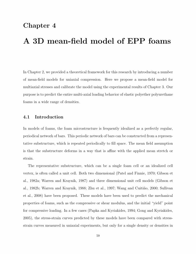
Chapter 4

A 3D mean-field model of EPP foams

In Chapter 2, we provided a theoretical framework for this research by introducing a number

of mean-field models for uniaxial compression. Here we propose a mean-field model for

multiaxial stresses and calibrate the model using the experimental results of Chapter 3. Our

purpose is to predict the entire multi-axial loading behavior of elastic polyether polyurethane

foams in a wide range of densities.

4.1 Introduction

In models of foams, the foam microstructure is frequently idealized as a perfectly regular,

periodical network of bars. This periodic network of bars can be constructed from a represen-

tative substructure, which is repeated periodically to fill space. The mean field assumption

is that the substructure deforms in a way that is affine with the applied mean stretch or

strain.

The representative substructure, which can be a single foam cell or an idealized cell

vertex, is often called a unit cell. Both two dimensional (Patel and Finnie, 1970; Gibson et

al., 1982a; Warren and Kraynik, 1987) and three dimensional unit cell models (Gibson et

al., 1982b; Warren and Kraynik, 1988; Zhu et al., 1997; Wang and Cuitino, 2000; Sullivan

et al., 2008) have been proposed. These models have been used to predict the mechanical

properties of foams, such as the compressive or shear modulus, and the initial “yield” point

for compressive loading. In a few cases (Papka and Kyriakides, 1994; Gong and Kyriakides,

2005), the stress-strain curves predicted by these models have been compared with stress-

strain curves measured in uniaxial experiments, but only for a single density or densities in

59

Z

Y

X

rise direction

(b)(a)

(c) (d)

hz

lx

hz

ly

lx

ly

X

Z

Y

Z

X

Y

L1

Lθ

Figure 4.1: The idealized foam representative microstructure. (a) 3D view of the foam microstructure. (b)Front view. (c) Side view. (d) Top view.

a very narrow range.

4.2 Formulation

4.2.1 Geometry of the model

The foam is idealized as a regular network of bars arranged as tetrahedral units (see Fig. 2.1a).

In each one of these four-bar tetrahedral cells, one bar of length L1 is aligned with the rise

direction of the foam and the other three bars of length L form an angle θ (in the undeformed

cell) with the rise direction (Fig. 4.1a).

The network of bars can be divided into different representative substructures that can

be packed to fill space without rotation. For the minimum representative substructure, see

Sabuwala et al. (2007); their unit cell contains 2 four-bar tetrahedral units, and occupies a

triangular prism in space.

Here we choose a representative substructure containing 16 four-bar tetrahedral units

60

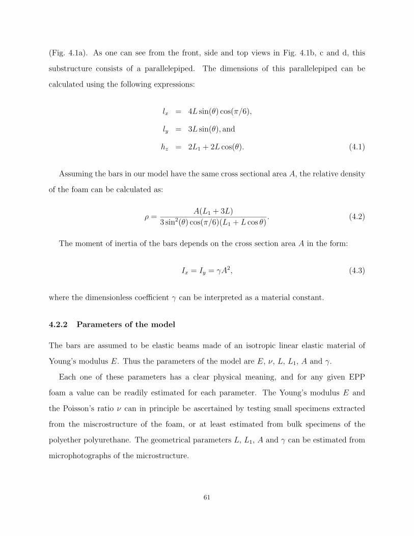
(Fig. 4.1a). As one can see from the front, side and top views in Fig. 4.1b, c and d, this

substructure consists of a parallelepiped. The dimensions of this parallelepiped can be

calculated using the following expressions:

lx = 4L sin(θ) cos(π/6),

ly = 3L sin(θ), and

hz = 2L1 + 2L cos(θ). (4.1)

Assuming the bars in our model have the same cross sectional area A, the relative density

of the foam can be calculated as:

ρ =A(L1 + 3L)

3 sin2(θ) cos(π/6)(L1 + L cos θ). (4.2)

The moment of inertia of the bars depends on the cross section area A in the form:

Ix = Iy = γA2, (4.3)

where the dimensionless coefficient γ can be interpreted as a material constant.

4.2.2 Parameters of the model

The bars are assumed to be elastic beams made of an isotropic linear elastic material of

Young’s modulus E. Thus the parameters of the model are E, ν, L, L1, A and γ.

Each one of these parameters has a clear physical meaning, and for any given EPP

foam a value can be readily estimated for each parameter. The Young’s modulus E and

the Poisson’s ratio ν can in principle be ascertained by testing small specimens extracted

from the miscrostructure of the foam, or at least estimated from bulk specimens of the

polyether polyurethane. The geometrical parameters L, L1, A and γ can be estimated from

microphotographs of the microstructure.

61

3+

x

y

z1−

1+

2−

2+

3−

Figure 4.2: The boundary faces of the substructure

4.2.3 Boundary conditions

The substructure is subjected to periodic boundary conditions. In our substructure, the

matching nodes are the couple of nodes which are on opposite boundary faces. For each pair

of boundary faces (Fig. 4.2), we choose a reference pair of matched nodes. With reference

nodes, the general periodic boundary conditions can be expressed as follows:

U j+i − U j−

i = U j+iref − U j−

iref

φj+i − φj−

i = φj+iref − φj−

iref (i, j = 1, 2, 3),(4.4)

where U is the displacement and φ is the rotation of the nodes. The subindex “i” represents

the direction of the displacement or rotation, and the prime index “j” represents the bound-

ary faces. Equation 4.4 indicates that on opposite boundary faces, the difference of the

displacements and rotations of matched nodes should be the same as that of the reference

nodes. A similar discussion of periodic boundary conditions can be found in Laroussi et al.

(2002).

4.2.4 Computational implementation

We use the Finite Element Analysis package ABAQUS for the computations. In the finite

element model, each bar of the substructure (Fig. 4.1) is represented with 8 beam elements

B32, which is a 3-node quadratic beam element. The B32 element allows large axial strains

62

as well as large rotations. It also allows transverse shear strains; that is, the cross-section

may not necessarily remain normal to the beam axis. The transverse shear strain is only

likely to be of any importance in the thick bars(Timoshenko, 1956) associated with foams

of high density.

4.3 Calibration

In this section we discuss the calibration of the model.

4.3.1 Calibration criteria

We calibrate the model by comparing the mechanical response given by the model against

the mechanical response measured in experiments (Chapter 3). For each loading case and

each density of the foam, we compare the theoretical and experimental stress-strain curves

(or force-displacement curves). If the strain energy function given by the model is nonconvex,

the function is properly convexified.

The objective of this calibration is to ascertain the capacity of the model to reproduce

the most salient features of the mechanical behavior of the series of commercial foams tested

in Chapter 4, over the whole range of relative densities of the foams, with emphasis on the

the physical mechanism whereby the deformation is effected at large strains. Therefore,

it is of particular importance to us that the model should give a nonconvex strain energy

function where (and only where) the experiments exhibit a stress plateau and two-phase

strain fields. This amounts to a requirement that the model should embody the correct

physics associated with a stress plateau and two-phase strain fields—that is to say, the

physics of phase transitions.

On the other hand, we place little emphasis on curve fitting in itself, because attain-

ing a perfect fit would require complicating the model in ways which are unrelated to the

basic physics of large-strain deformation in EPP foams. Thus, for example, attaining a

good fit at small strains would require the use of a nonlinear constitutive relation for the

63

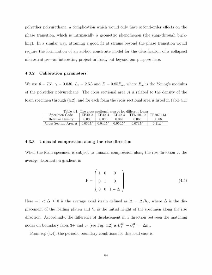
polyether polyurethane, a complication which would only have second-order effects on the

phase transition, which is intrinsically a geometric phenomenon (the snap-through buck-

ling). In a similar way, attaining a good fit at strains beyond the phase transition would

require the formulation of an ad-hoc constitute model for the densification of a collapsed

microstruture—an interesting project in itself, but beyond our purpose here.

4.3.2 Calibration parameters

We use θ = 76o, γ = 0.036, L1 = 2.5L and E = 0.85Em, where Em is the Young’s modulus

of the polyether polyurethane. The cross sectional area A is related to the density of the

foam specimen through (4.2), and for each foam the cross sectional area is listed in table 4.1:

Table 4.1: The cross sectional area A for different foamsSpecimen Code EF4003 EF4004 EF4005 TF5070-10 TF5070-13Relative Density 0.030 0.038 0.046 0.065 0.086

Cross Section Area A 0.036L2 0.046L2 0.056L2 0.079L2 0.11L2

4.3.3 Uniaxial compression along the rise direction

When the foam specimen is subject to uniaxial compression along the rise direction z, the

average deformation gradient is

F =

1 0 0

0 1 0

0 0 1 + ∆

. (4.5)

Here −1 < ∆ ≤ 0 is the average axial strain defined as ∆ = ∆/hz, where ∆ is the dis-

placement of the loading platen and hz is the initial height of the specimen along the rise

direction. Accordingly, the difference of displacement in z direction between the matching

nodes on boundary faces 3+ and 3- (see Fig. 4.2) is U3+3 − U3−

3 = ∆hz.

From eq. (4.4), the periodic boundary conditions for this load case is:

64

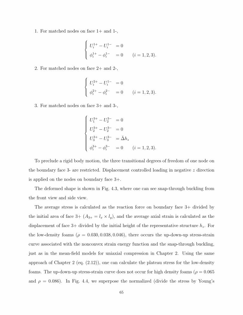
1. For matched nodes on face 1+ and 1-,

U1+i − U1−

i = 0

φ1+i − φ1−

i = 0 (i = 1, 2, 3).

2. For matched nodes on face 2+ and 2-,

U2+i − U1−

i = 0

φ2+i − φ2−

i = 0 (i = 1, 2, 3).

3. For matched nodes on face 3+ and 3-,

U3+1 − U3−

2 = 0

U3+2 − U3−

2 = 0

U3+3 − U3−

3 = ∆hz

φ3+i − φ3−

i = 0 (i = 1, 2, 3).

To preclude a rigid body motion, the three transitional degrees of freedom of one node on

the boundary face 3- are restricted. Displacement controlled loading in negative z direction

is applied on the nodes on boundary face 3+.

The deformed shape is shown in Fig. 4.3, where one can see snap-through buckling from

the front view and side view.

The average stress is calculated as the reaction force on boundary face 3+ divided by

the initial area of face 3+ (A3+ = lx × ly), and the average axial strain is calculated as the

displacement of face 3+ divided by the initial height of the representative structure hz. For

the low-density foams (ρ = 0.030, 0.038, 0.046), there occurs the up-down-up stress-strain

curve associated with the nonconvex strain energy function and the snap-through buckling,

just as in the mean-field models for uniaxial compression in Chapter 2. Using the same

approach of Chapter 2 (eq. (2.12)), one can calculate the plateau stress for the low-density

foams. The up-down-up stress-strain curve does not occur for high density foams (ρ = 0.065

and ρ = 0.086). In Fig. 4.4, we superpose the normalized (divide the stress by Young’s

65

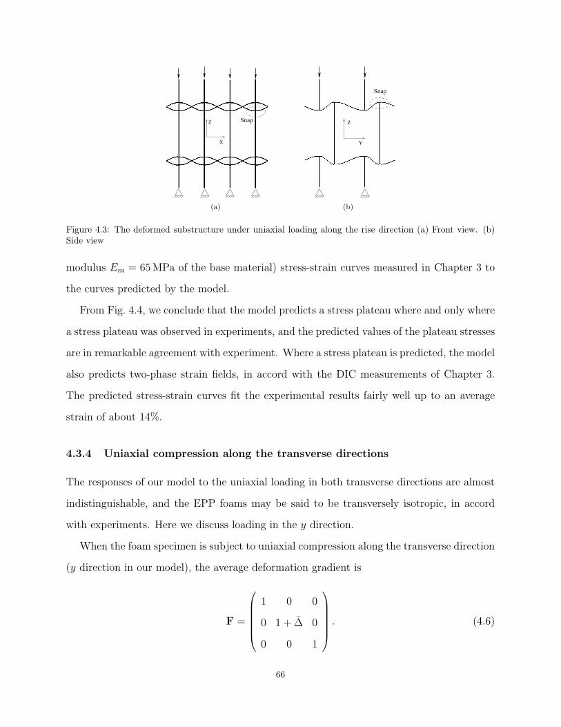
Z

X

Snap

(a)

Z

Y

Snap

(b)

Figure 4.3: The deformed substructure under uniaxial loading along the rise direction (a) Front view. (b)Side view

modulus Em = 65 MPa of the base material) stress-strain curves measured in Chapter 3 to

the curves predicted by the model.

From Fig. 4.4, we conclude that the model predicts a stress plateau where and only where

a stress plateau was observed in experiments, and the predicted values of the plateau stresses

are in remarkable agreement with experiment. Where a stress plateau is predicted, the model

also predicts two-phase strain fields, in accord with the DIC measurements of Chapter 3.

The predicted stress-strain curves fit the experimental results fairly well up to an average

strain of about 14%.

4.3.4 Uniaxial compression along the transverse directions

The responses of our model to the uniaxial loading in both transverse directions are almost

indistinguishable, and the EPP foams may be said to be transversely isotropic, in accord

with experiments. Here we discuss loading in the y direction.

When the foam specimen is subject to uniaxial compression along the transverse direction

(y direction in our model), the average deformation gradient is

F =

1 0 0

0 1 + ∆ 0

0 0 1

. (4.6)

66

0.00 0.04 0.08 0.12 0.16 0.200.0000

0.0002

0.0004

0.0006

0.0008

0.0010

0.0012

0.0014

Numerical Experimental

=0.086

=0.065

=0.046

=0.038

Nor

mal

ized

Stre

ss

Axial Strain

=0.030

Figure 4.4: The experimental and predicted response of foam specimens for uniaxial compression along therise direction

Here −1 < ∆ ≤ 0 is the average axial strain defined as ∆ = ∆/ly, where ∆ is the compression

and ly is the initial height of the specimen along the rise direction. Accordingly, the difference

of displacement in y direction between the matching nodes on boundary faces 2+ and 2-

(see Fig. 4.2) is U2+2 − U2−

2 = ∆ly.

From eq. (4.4), the periodic boundary conditions for this load case is:

1. For matched nodes on face 1+ and 1-,

U1+i − U1−

i = 0

φ1+i − φ1−

i = 0 (i = 1, 2, 3).

2. For matched nodes on face 2+ and 2-,

U2+1 − U2−

2 = 0

U2+2 − U2−

2 = ∆ly

U2+3 − U2−

3 = 0

φ2+i − φ2−

i = 0 (i = 1, 2, 3).

67

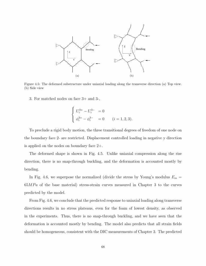
Z

Y

Bending

(a)

Z

Y

Bending

(b)

Figure 4.5: The deformed substructure under uniaxial loading along the transverse direction (a) Top view.(b) Side view

3. For matched nodes on face 3+ and 3-,

U3+i − U3−

i = 0

φ3+i − φ3−

i = 0 (i = 1, 2, 3).

To preclude a rigid body motion, the three transitional degrees of freedom of one node on

the boundary face 2- are restricted. Displacement controlled loading in negative y direction

is applied on the nodes on boundary face 2+.

The deformed shape is shown in Fig. 4.5. Unlike uniaxial compression along the rise

direction, there is no snap-through buckling, and the deformation is accounted mostly by

bending.

In Fig. 4.6, we superpose the normalized (divide the stress by Young’s modulus Em =

65MPa of the base material) stress-strain curves measured in Chapter 3 to the curves

predicted by the model.

From Fig. 4.6, we conclude that the predicted response to uniaxial loading along transverse

directions results in no stress plateaus, even for the foam of lowest density, as observed

in the experiments. Thus, there is no snap-through buckling, and we have seen that the

deformation is accounted mostly by bending. The model also predicts that all strain fields

should be homogeneous, consistent with the DIC measurements of Chapter 3. The predicted

68

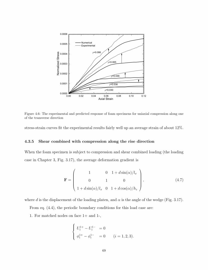
0.00 0.02 0.04 0.06 0.08 0.10 0.120.0000

0.0001

0.0002

0.0003

0.0004

0.0005

0.0006

Numerical Experimental

=0.086

=0.065

=0.046

=0.038

Nor

mal

ized

Stre

ss

Axial Strain

=0.030

Figure 4.6: The experimental and predicted response of foam specimens for uniaxial compression along oneof the transverse direction

stress-strain curves fit the experimental results fairly well up an average strain of about 12%.

4.3.5 Shear combined with compression along the rise direction

When the foam specimen is subject to compression and shear combined loading (the loading

case in Chapter 3, Fig. 3.17), the average deformation gradient is

F =

1 0 1 + d sin(α)/lx

0 1 0

1 + d sin(α)/lx 0 1 + d cos(α)/hz

, (4.7)

where d is the displacement of the loading platen, and α is the angle of the wedge (Fig. 3.17).

From eq. (4.4), the periodic boundary conditions for this load case are:

1. For matched nodes on face 1+ and 1-,

U1+i − U1−

i = 0

φ1+i − φ1−

i = 0 (i = 1, 2, 3).

69

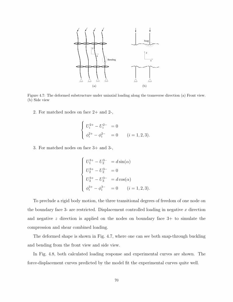
Z

X

Bending

(a)

Z

Y

Snap

(b)

Figure 4.7: The deformed substructure under uniaxial loading along the transverse direction (a) Front view.(b) Side view

2. For matched nodes on face 2+ and 2-,

U2+i − U2−

i = 0

φ2+i − φ2−

i = 0 (i = 1, 2, 3).

3. For matched nodes on face 3+ and 3-,

U3+1 − U3−

2 = d sin(α)

U3+2 − U3−

2 = 0

U3+3 − U3−

3 = d cos(α)

φ3+i − φ3−

i = 0 (i = 1, 2, 3).

To preclude a rigid body motion, the three transitional degrees of freedom of one node on

the boundary face 3- are restricted. Displacement controlled loading in negative x direction

and negative z direction is applied on the nodes on boundary face 3+ to simulate the

compression and shear combined loading.

The deformed shape is shown in Fig. 4.7, where one can see both snap-through buckling

and bending from the front view and side view.

In Fig. 4.8, both calculated loading response and experimental curves are shown. The

force-displacement curves predicted by the model fit the experimental curves quite well.

70

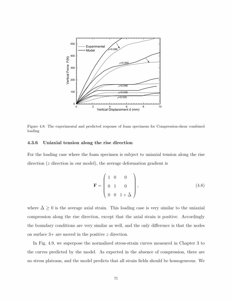
0 2 4 6 8 100

100

200

300

400

500 Experimental Model =0.086

=0.065

=0.046

=0.038

Ver

tical

For

ce F

(N)

Vertical Displacement d (mm)

=0.030

Figure 4.8: The experimental and predicted response of foam specimens for Compression-shear combinedloading

4.3.6 Uniaxial tension along the rise direction

For the loading case where the foam specimen is subject to uniaxial tension along the rise

direction (z direction in our model), the average deformation gradient is

F =

1 0 0

0 1 0

0 0 1 + ∆

, (4.8)

where ∆ ≥ 0 is the average axial strain. This loading case is very similar to the uniaxial

compression along the rise direction, except that the axial strain is positive. Accordingly

the boundary conditions are very similar as well, and the only difference is that the nodes

on surface 3+ are moved in the positive z direction.

In Fig. 4.9, we superpose the normalized stress-strain curves measured in Chapter 3 to

the curves predicted by the model. As expected in the absence of compression, there are

no stress plateaus, and the model predicts that all strain fields should be homogeneous. We

71

0.00 0.02 0.04 0.06 0.08 0.100.0000

0.0004

0.0008

0.0012

0.0016

=0.086 =0.065

=0.046=0.038

Numerical Experimental

Nor

mal

ized

Stre

ss

Axial Strain

=0.030

Figure 4.9: The experimental and predicted response for uniaxial tension along the rise direction

interpret the slight softening apparent in the stress-strain curves measured in experiments

as signatures of the development of damage in the microstructure of the foams.

4.3.7 Triaxial loading

Similar to experiments, the triaxial loading is modeled as a two-step process. First, con-

finement hydrostatic pressure is applied. Second, the displacement in x and y directions

(transverse directions) of the side surfaces are fixed, while the top surface (surface 3+) is

subject to displacement in negative z direction (the compression in the rise direction).

In Fig. 4.10, we compare the measured and predicted axial stress-strain curves. The

predicted curves do not fit the experiments as well as the other four loading cases, but

the model is able to predict the most notable trends, such as the occurrence of the stress

plateaus, and the drop of the plateau stress with the increase of confinement pressure.

72

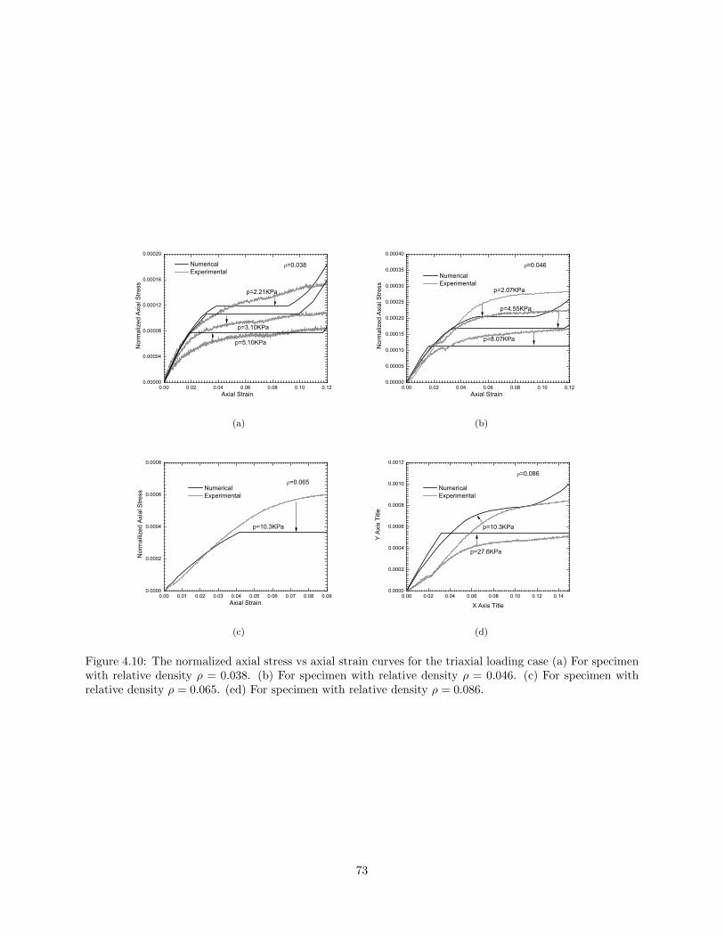
0.00 0.02 0.04 0.06 0.08 0.10 0.120.00000

0.00004

0.00008

0.00012

0.00016

0.00020

Numerical Experimental

p=5.10KPa

Nor

mal

ized

Axi

al S

tress

Axial Strain

=0.038

p=2.21KPa

p=3.10KPa

(a)

0.00 0.02 0.04 0.06 0.08 0.10 0.120.00000

0.00005

0.00010

0.00015

0.00020

0.00025

0.00030

0.00035

0.00040

Numerical Experimental

p=8.07KPa

p=4.55KPa

Nor

mal

ized

Axi

al S

tress

Axial Strain

=0.046

p=2.07KPa

(b)

0.00 0.01 0.02 0.03 0.04 0.05 0.06 0.07 0.08 0.090.0000

0.0002

0.0004

0.0006

0.0008

p=10.3KPa

Numerical Experimental

Nor

mai

lized

Axi

al S

tress

Axial Strain

=0.065

(c)

0.00 0.02 0.04 0.06 0.08 0.10 0.12 0.140.0000

0.0002

0.0004

0.0006

0.0008

0.0010

0.0012

Numerical Experimental

p=27.6KPa

Y A

xis

Title

X Axis Title

=0.086

p=10.3KPa

(d)

Figure 4.10: The normalized axial stress vs axial strain curves for the triaxial loading case (a) For specimenwith relative density ρ = 0.038. (b) For specimen with relative density ρ = 0.046. (c) For specimen withrelative density ρ = 0.065. (ed) For specimen with relative density ρ = 0.086.

73

4.4 Discussion

The mechanical behavior of EPP foams under uniaxial stretch exhibits stress plateaus and

heterogeneous, two-phase strain fields for low-density foams; a critical point for foams of

critical density; and hardening accompanied by homogeneous strain fields for high-density

foams. Thus, even under the simplest loading, a vast phenomenological universe accompanies

the deformation of EPP foams up to large strains. And yet, as we have shown in Chapter 2,

all of the most salient features of this vast phenomenological universe can be described

using a simple mean-field model. In this simple mean-field model, an idealized cell of the

microstructure of the foam is subjected to displacements affine to the applied mean strain

and used to compute a strain energy function. For low-density foams, where the bars that

constitute the idealized cell are relatively slender, the cell attains a limit point and undergoes

snap-through buckling; as a result, the strain energy function is nonconvex. The nonconvex

strain energy function can be convexified using conventional tools of analysis, and the results

confer a straightforward theoretical interpretation to the most salient structural features of

the mechanical response of EEP foams subjected to uniaxial loading: the stress plateaus,

the two-phase strain fields, the critical point, etc. Further, the mean-field model yields

theoretical stress-strain curves which fit well the stress-strain curves measured in experiment

for a complete series of commercially available EPP foams subjected to uniaxial stretching.

In particular, the predicted values of the plateau stresses for foams of different densities are

in very good accord with the values measured in experiments.

In this chapter, we have extended the work of Chapter 2 to show that a 3D generalization

of the mean-field model of Chapter 2 can account in a similar way for the experimental re-

sults Chapter 3, where the mechanical response of EPP foams was measured for five different

loading cases. These loading cases are uniaxial compression along the rise direction, uniax-

ial compression along the transverse directions, compression-shear combined with uniaxial

tension along the rise direction, and triaxial loading.

Each of the few geometrical or material parameters of the 3D mean-field model has a

74

clear physical meaning related to the microstructure of a foam. Using a single set of values

of these parameters, we have verified that for all five loading cases and each of the foams

in a commercially available series of EPP foams, the model gives a nonconvex strain energy

function where (and only where) the experiments exhibit a stress plateau and heterogeneous,

two-phase strain fields. These results lend a straightforward theoretical interpretation to the

most salient structural features of the mechanical response observed experimentally in EEP

foams of a wide range of densities, and for a variety of multiaxial loading cases.

By means of a comparison of the predicted and measured plateau stresses (the sole crite-

rion by which models have been evaluated in the past, invariably for a few foams of similar

densities subjected to uniaxial loading), we have shown that the 3D mean-field model gives

remarkably accurate predictions of all plateau stresses with the exception of the plateau

stresses of the triaxial loading case, where the predicted plateau stresses are off by up to

30% for some foams. Even though we have not made a particular effort at curve fitting (cf.

Section 4.3.1), we have seen from an unprecedented comparison of the complete, predicted

and measured stress-strain curves for each loading case and each foam, that the model gives

a remarkably good fit for most loading cases. The only exception is once more the triaxial

loading case, where the fits can be said to be reasonable.

We close this chapter with a few remarks on the evaluation of the goodness of a model

of EPP foams. To the best of our knowledge, we are the first to have compared measured

and predicted stress-strain curves for numerous loading cases and a complete series of foams

of widely differing densities. This practice must become common place if we are to provide

a reliable simulation tool for engineering applications. In this respect, our 3D model would

benefit from further work aimed, for example, at attaining a better fit at small strains through

the introduction of a suitable nonlinear constitutive relation for the polyether polyurethane.

We would like to emphasize, however, that the goodness of a model can hardly consist

in the capacity of the model to give excellent fits to numerous stress-strain curves measured

in experiments. Instead, the most important criterion of goodness is that a model should

embody the correct physics associated with the most salient features of the mechanical

75

response observed in experiments. For EEP foams, these most salient features are the stress

plateaus and the attendant two-phase strain fields.

In this respect, note that a stress plateau can be modeled using continuum plasticity. This

has been a common practice in the automotive industry, where continuum plasticity models

of EPP foams are customarily used to perform computational simulations of seat–passenger

interactions that take place during a crash. And yet, in continuum plasticity a stress plateau

is not accompanied by two-phase strain fields.

A stress plateau can also ensue from Euler buckling, and in most models of EPP foams

the stress plateaus are associated with a bifurcation of equilibrium of the microstructure

of the foam. Where the microstructure of a foam undergoes Euler buckling, the attendant

strain field will correspond to an eigenfunction of arbitrary amplitude. As the applied mean

strain is increased following buckling, the stress-strain curve traces a stress plateau, and the

strain field remains invariant except for the amplitude, which increases to accommodate the

applied mean strain. This scenario is inconsistent with the conjunction of a stress plateau

and two-phase fields observed in experiments, where an increasing applied mean strain is

accommodated by growth of the volume fraction of the high-density phase at the expense of

the volume fraction of the low-density phase.

The leitmotif of this chapter has been a focus on the most distinctive structural feature

of the mechanical response of EPP foams evinced in experiments: the conjunction of a

stress plateau and two-phase fields. This conjunction signals the prevalence of a phase

transition, which is the basic physics of large-strain deformation in EPP foams. Thus, in

judging the performance of our model, we have emphasized the capacity of the model to give

a nonconvex strain energy function—the signature of a phase transition—where (and only

where) the experiments exhibit a stress plateau and two-phase strain fields. This emphasis

should remain a guiding methodological trait in the design of constitutive models of EPP

foams.

76

Chapter 5

Punching elastic foams in theself-similar regime

5.1 Introduction

Polyether polyurethane foams are used in packaging, for example, to protect merchandize

in shipping, transportation, and handling. Polyether polyurethane foams are also used in

car seats to provide comfort and safety to car occupants. In these applications and many

similar ones, the purpose of the foam is to react to outside forces that impinge on the foam.

For example, when a car occupant is seated in a car, his legs, back, and buttocks impinge

on the foam of the seat. In this example, the occupant’s legs and back may be thought

of as cylindrical punches, and the buttocks as spherical punches. Thus, it is of interest to

determine what happens when a punch penetrates an elastic foam, and how the foam reacts

mechanically.

Here we investigate experimentally the mechanical behavior of polyether polyurethane

foams being penetrated by a rigid punch (i.e., a punch made of a material that is much

stiffer than the foams). We use two types of punches of simple geometry: a wedge-shaped

punch and a conical punch. We also perform a theoretical analysis of the experiments and

show the predictions to be in good agreement with the experimental measurements.

5.2 Experimental set-up

The experimental set-up consists of an ATS testing machine (Fig. 3.1) that is used to drive

the punch into the foam specimen at a constant velocity. During an experiment, the punch is

attached to a load cell whose signal is fed to a computer running the LabView software. This

77

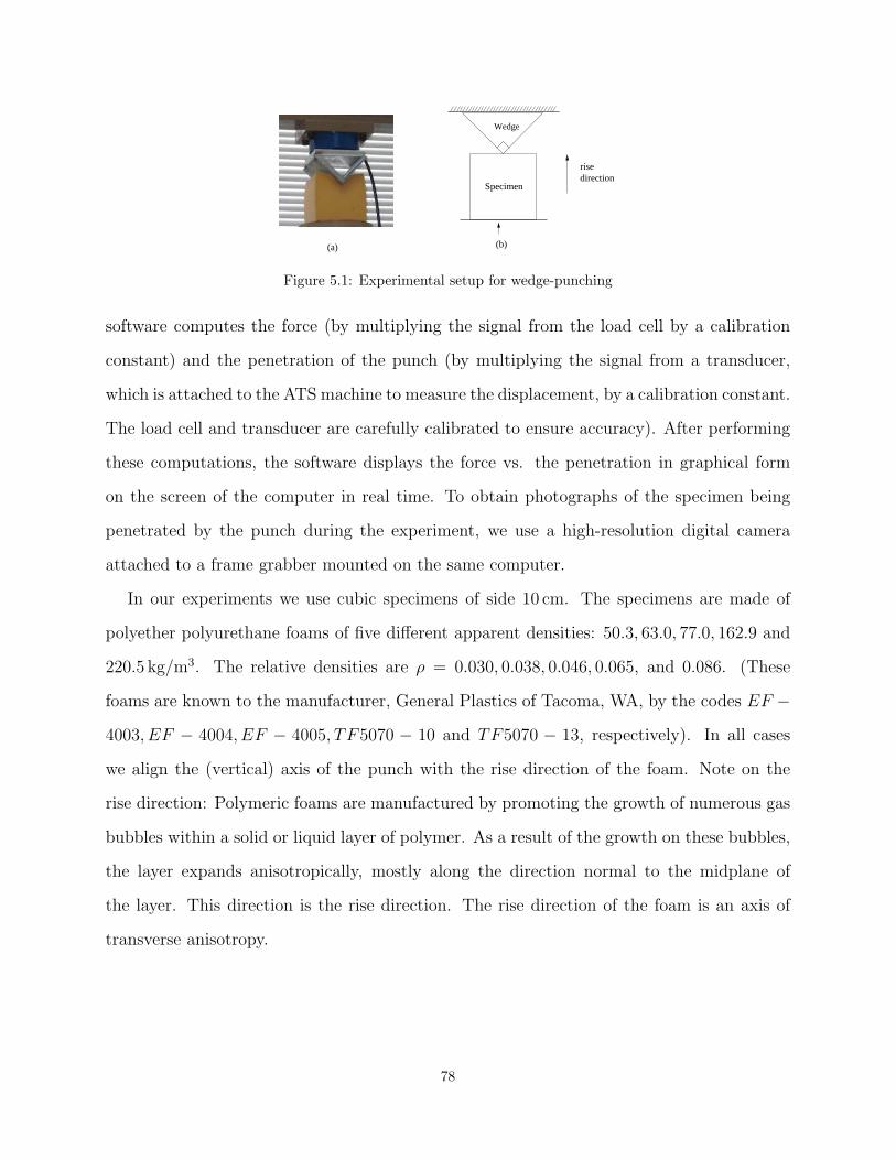
(a)

Specimen

Wedge

rise direction

(b)

Figure 5.1: Experimental setup for wedge-punching

software computes the force (by multiplying the signal from the load cell by a calibration

constant) and the penetration of the punch (by multiplying the signal from a transducer,

which is attached to the ATS machine to measure the displacement, by a calibration constant.

The load cell and transducer are carefully calibrated to ensure accuracy). After performing

these computations, the software displays the force vs. the penetration in graphical form

on the screen of the computer in real time. To obtain photographs of the specimen being

penetrated by the punch during the experiment, we use a high-resolution digital camera

attached to a frame grabber mounted on the same computer.

In our experiments we use cubic specimens of side 10 cm. The specimens are made of

polyether polyurethane foams of five different apparent densities: 50.3, 63.0, 77.0, 162.9 and

220.5 kg/m3. The relative densities are ρ = 0.030, 0.038, 0.046, 0.065, and 0.086. (These

foams are known to the manufacturer, General Plastics of Tacoma, WA, by the codes EF −4003, EF − 4004, EF − 4005, TF5070 − 10 and TF5070 − 13, respectively). In all cases

we align the (vertical) axis of the punch with the rise direction of the foam. Note on the

rise direction: Polymeric foams are manufactured by promoting the growth of numerous gas

bubbles within a solid or liquid layer of polymer. As a result of the growth on these bubbles,

the layer expands anisotropically, mostly along the direction normal to the midplane of

the layer. This direction is the rise direction. The rise direction of the foam is an axis of

transverse anisotropy.

78

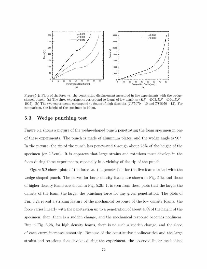
0 10 20 30 40 50 60 70 800

50

100

150

200

250

300

350

0 10 20 30 40 50 60 70 800

500

1000

1500

2000

2500

3000

3500

(b)

=0.030 =0.038 =0.046

Forc

e(N

)

Penetration Depth(mm)(a)

=0.065 =0.086

Forc

e(N

)

Penetration Depth(mm)

Figure 5.2: Plots of the force vs. the penetration displacement measured in five experiments with the wedge-shaped punch. (a) The three experiments correspond to foams of low densities (EF −4003, EF −4004, EF −4005). (b) The two experiments correspond to foams of high densities (TF5070− 10 and TF5070− 13). Forcomparison, the height of the specimen is 10 cm.

5.3 Wedge punching test

Figure 5.1 shows a picture of the wedge-shaped punch penetrating the foam specimen in one

of these experiments. The punch is made of aluminum plates, and the wedge angle is 90 ◦.

In the picture, the tip of the punch has penetrated through about 25% of the height of the

specimen (or 2.5 cm). It is apparent that large strains and rotations must develop in the

foam during these experiments, especially in a vicinity of the tip of the punch.

Figure 5.2 shows plots of the force vs. the penetration for the five foams tested with the

wedge-shaped punch. The curves for lower density foams are shown in Fig. 5.2a and those

of higher density foams are shown in Fig. 5.2b. It is seen from these plots that the larger the

density of the foam, the larger the punching force for any given penetration. The plots of

Fig. 5.2a reveal a striking feature of the mechanical response of the low density foams: the

force varies linearly with the penetration up to a penetration of about 40% of the height of the

specimen; then, there is a sudden change, and the mechanical response becomes nonlinear.

But in Fig. 5.2b, for high density foams, there is no such a sudden change, and the slope

of each curve increases smoothly. Because of the constitutive nonlinearities and the large

strains and rotations that develop during the experiment, the observed linear mechanical

79

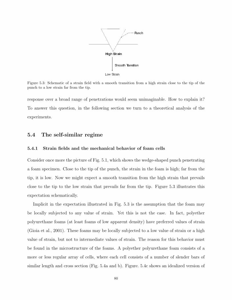
Figure 5.3: Schematic of a strain field with a smooth transition from a high strain close to the tip of thepunch to a low strain far from the tip.

response over a broad range of penetrations would seem unimaginable. How to explain it?

To answer this question, in the following section we turn to a theoretical analysis of the

experiments.

5.4 The self-similar regime

5.4.1 Strain fields and the mechanical behavior of foam cells

Consider once more the picture of Fig. 5.1, which shows the wedge-shaped punch penetrating

a foam specimen. Close to the tip of the punch, the strain in the foam is high; far from the

tip, it is low. Now we might expect a smooth transition from the high strain that prevails

close to the tip to the low strain that prevails far from the tip. Figure 5.3 illustrates this

expectation schematically.

Implicit in the expectation illustrated in Fig. 5.3 is the assumption that the foam may

be locally subjected to any value of strain. Yet this is not the case. In fact, polyether

polyurethane foams (at least foams of low apparent density) have preferred values of strain

(Gioia et al., 2001). These foams may be locally subjected to a low value of strain or a high

value of strain, but not to intermediate values of strain. The reason for this behavior must

be found in the microstructure of the foams. A polyether polyurethane foam consists of a

more or less regular array of cells, where each cell consists of a number of slender bars of

similar length and cross section (Fig. 5.4a and b). Figure. 5.4c shows an idealized version of

80

this array of identical cells. Now the cells of a foam subjected to a compressive strain act

structurally as slender, shallow arches. When a load is applied to a slender, shallow arch, the

deformation of the arch increases smoothly as the load is increased, but only up to a certain

limit load. Then, if the load is increased beyond the limit load, the deformation of the arch

jumps discontinuously to a much higher level. This mechanical phenomenon, called “snap-

through buckling” by structural engineers, implies that foams have two preferred values of

strain: a low value of strain associated with the configuration of the cells before snap-through

buckling (Fig. 5.4c) and a large value of strain associated with the configuration of the cells

after snap-through buckling (Fig. 5.4d). Because they undergo snap-through buckling when

compressed, the cells of foams may be termed bi-stable elastic structures. (For a pioneering

study of the snap-through bulking in foams, see Lakes et al. (1993)). Even though we may

be unaware of it, bi-stable elastic structures are frequently encountered in everyday life. For

example, the cap of a shampoo bottle is a bi-stable elastic structure: the cap is always either

closed (as in Fig. 5.4e, which should be compared with Fig. 5.4c) or open (as in Fig. 5.4f,

which should be compared with Fig. 5.4d), but not partially open or partially closed.

5.4.2 The self-similar regime

Let us now discuss how the sharp interface evolves during an experiment with a wedge-

shaped punch. For simplicity, we assume that the sharp interface is a semi-cylinder of radius

R, as shown in Fig. 5.5(a). As the penetration increases, we expect that R should increase

too (Fig. 5.5(b)). Since there is no characteristic length in the wedge-shaped punch, the

only prevailing length scale is the penetration d. Thus the radius R of the sharp interface

must be proportional to the penetration d of the punch, as illustrated in Fig. 5.5. As the

penetration increases during the test, the radius of the sharp interface increases in direct

proportion to the penetration. This we call the self-similar regime, because in this regime

the sharp interface remains similar to itself (it is always a semi-cylinder). The self-similar

regime prevails until the sharp interface reaches the side or bottom of the specimen. After

the sharp interface has reached the side or bottom of the specimen, a new length scale,

81

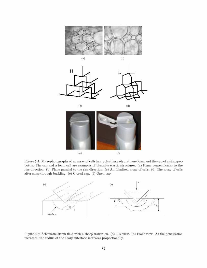
(a) (b)

(c) (d)

(e) (f)

Figure 5.4: Microphotographs of an array of cells in a polyether polyurethane foam and the cap of a shampoobottle. The cap and a foam cell are examples of bi-stable elastic structures. (a) Plane perpendicular to therise direction. (b) Plane parallel to the rise direction. (c) An Idealized array of cells. (d) The array of cellsafter snap-through buckling. (e) Closed cap. (f) Open cap.

(b)F

θdR d’R’

HL

interface

(a)

Figure 5.5: Schematic strain field with a sharp transition. (a) 3-D view. (b) Front view. As the penetrationincreases, the radius of the sharp interface increases proportionally.

82

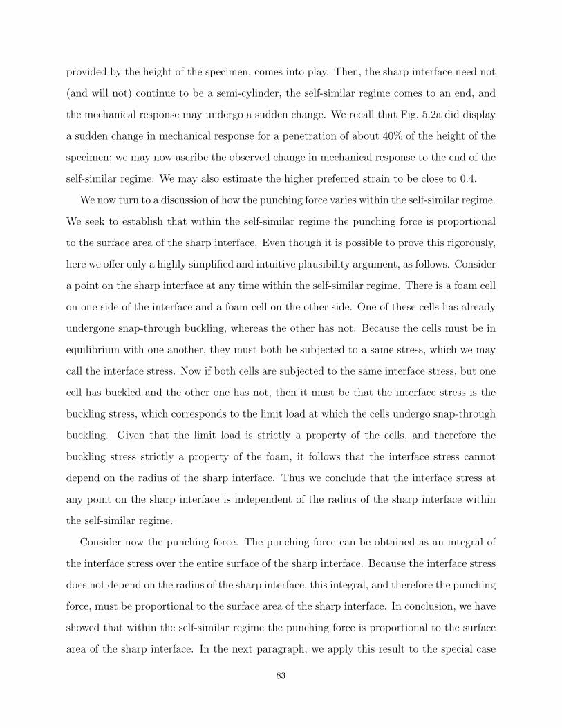
provided by the height of the specimen, comes into play. Then, the sharp interface need not

(and will not) continue to be a semi-cylinder, the self-similar regime comes to an end, and

the mechanical response may undergo a sudden change. We recall that Fig. 5.2a did display

a sudden change in mechanical response for a penetration of about 40% of the height of the

specimen; we may now ascribe the observed change in mechanical response to the end of the

self-similar regime. We may also estimate the higher preferred strain to be close to 0.4.

We now turn to a discussion of how the punching force varies within the self-similar regime.

We seek to establish that within the self-similar regime the punching force is proportional

to the surface area of the sharp interface. Even though it is possible to prove this rigorously,

here we offer only a highly simplified and intuitive plausibility argument, as follows. Consider

a point on the sharp interface at any time within the self-similar regime. There is a foam cell

on one side of the interface and a foam cell on the other side. One of these cells has already

undergone snap-through buckling, whereas the other has not. Because the cells must be in

equilibrium with one another, they must both be subjected to a same stress, which we may

call the interface stress. Now if both cells are subjected to the same interface stress, but one

cell has buckled and the other one has not, then it must be that the interface stress is the

buckling stress, which corresponds to the limit load at which the cells undergo snap-through

buckling. Given that the limit load is strictly a property of the cells, and therefore the

buckling stress strictly a property of the foam, it follows that the interface stress cannot

depend on the radius of the sharp interface. Thus we conclude that the interface stress at

any point on the sharp interface is independent of the radius of the sharp interface within

the self-similar regime.

Consider now the punching force. The punching force can be obtained as an integral of

the interface stress over the entire surface of the sharp interface. Because the interface stress

does not depend on the radius of the sharp interface, this integral, and therefore the punching

force, must be proportional to the surface area of the sharp interface. In conclusion, we have

showed that within the self-similar regime the punching force is proportional to the surface

area of the sharp interface. In the next paragraph, we apply this result to the special case

83

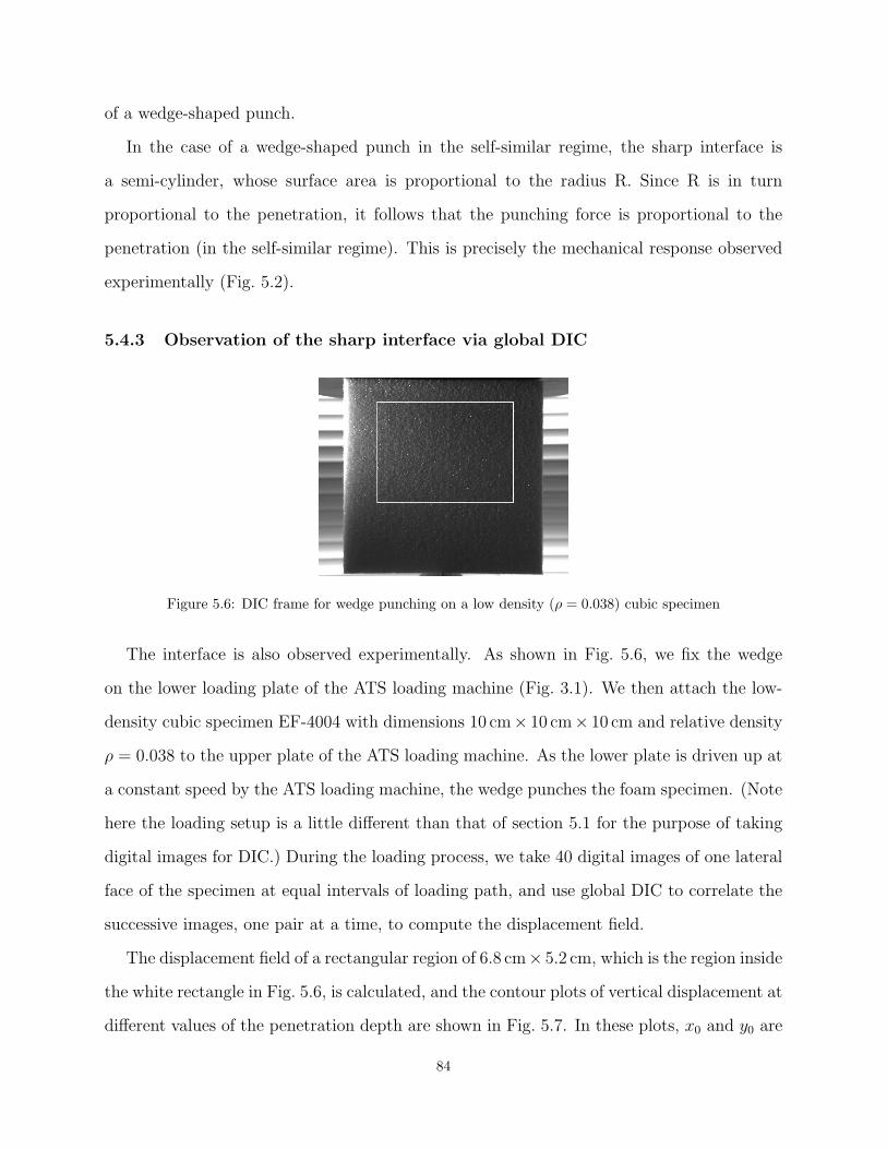
of a wedge-shaped punch.

In the case of a wedge-shaped punch in the self-similar regime, the sharp interface is

a semi-cylinder, whose surface area is proportional to the radius R. Since R is in turn

proportional to the penetration, it follows that the punching force is proportional to the

penetration (in the self-similar regime). This is precisely the mechanical response observed

experimentally (Fig. 5.2).

5.4.3 Observation of the sharp interface via global DIC

Figure 5.6: DIC frame for wedge punching on a low density (ρ = 0.038) cubic specimen

The interface is also observed experimentally. As shown in Fig. 5.6, we fix the wedge

on the lower loading plate of the ATS loading machine (Fig. 3.1). We then attach the low-

density cubic specimen EF-4004 with dimensions 10 cm× 10 cm× 10 cm and relative density

ρ = 0.038 to the upper plate of the ATS loading machine. As the lower plate is driven up at

a constant speed by the ATS loading machine, the wedge punches the foam specimen. (Note

here the loading setup is a little different than that of section 5.1 for the purpose of taking

digital images for DIC.) During the loading process, we take 40 digital images of one lateral

face of the specimen at equal intervals of loading path, and use global DIC to correlate the

successive images, one pair at a time, to compute the displacement field.

The displacement field of a rectangular region of 6.8 cm× 5.2 cm, which is the region inside

the white rectangle in Fig. 5.6, is calculated, and the contour plots of vertical displacement at

different values of the penetration depth are shown in Fig. 5.7. In these plots, x0 and y0 are

84

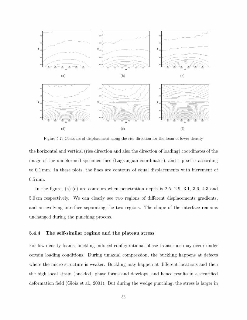
X0

Y0

400 500 600 700 800 900

200

300

400

500

600

(a)

X0

Y0

400 500 600 700 800 900

200

300

400

500

600

(b)

X0

Y0

400 500 600 700 800 900

200

300

400

500

600

(c)

X0

Y0

400 500 600 700 800 900

200

300

400

500

600

(d)

X0

Y0

400 500 600 700 800 900

200

300

400

500

600

(e)

X0

Y0

400 500 600 700 800 900

200

300

400

500

600

(f)

Figure 5.7: Contours of displacement along the rise direction for the foam of lower density

the horizontal and vertical (rise direction and also the direction of loading) coordinates of the

image of the undeformed specimen face (Lagrangian coordinates), and 1 pixel is according

to 0.1 mm. In these plots, the lines are contours of equal displacements with increment of

0.5 mm.

In the figure, (a)-(e) are contours when penetration depth is 2.5, 2.9, 3.1, 3.6, 4.3 and

5.0 cm respectively. We can clearly see two regions of different displacements gradients,

and an evolving interface separating the two regions. The shape of the interface remains

unchanged during the punching process.

5.4.4 The self-similar regime and the plateau stress

For low density foams, buckling induced configurational phase transitions may occur under

certain loading conditions. During uniaxial compression, the buckling happens at defects

where the micro structure is weaker. Buckling may happen at different locations and then

the high local strain (buckled) phase forms and develops, and hence results in a stratified

deformation field (Gioia et al., 2001). But during the wedge punching, the stress is larger in

85

the region closer to the wedge punch, so the high strain (buckled) phase forms at the punch

tip, and grows into the specimen when the punching continues. There should be a sharp

interface during the process to separate the two phases (Fig. 5.5a).

The wedge punching process can be simplified to a 2-D problem, since the interface is

a part of some kind of cylinder (not necessarily with a circular cross section), and can

be represented by a curve (Fig. 5.5b) of function r(θ) = RΘ(θ), where r and θ are polar

coordinates and R represents the length scale of the curve, while the dimensionless function

Θ(θ) gives the shape of the curve. Since during the punching process, the only prevailing

length scale is the penetration depth d, R must increase proportionally to d. In Fig. 5.5b,

as the penetration increases from d to d′, the curve that represents the interface becomes

r′(θ) = R′Θ(θ), and R/d = R′/d′ = c1, where c1 is a constant. Note here we have assumed

the self-similar evolvement of the interface. (The spatial self-similarity of contact for isotropic

linear elastic materials was established by (Galanov, 1981) and (Borodich, 1983), for non-

linear power-law materials, it was discovered by (Galanov, 1981) and (Borodich, 1989) in

isotropic and anisotropic cases respectively.)

We know that in the uniaxial case the configurational phase transition occurs when the

condition σ = σp is satisfied. We can assume a similar buckling condition for multiaxial cases,

f(σ1, σ2, σ3) = σy, where σy is a material constant, σ1, σ2, and σ3 are principal stresses,

and f(σ1, σ2, σ3) is a homogeneous function of order one on the magnitude of the stress

tensor |σ|, i.e., f(nσ1, nσ2, nσ3) = nf(σ1, σ2, σ3), where n is a constant scalar. Due to self

similarity, at points (r, θ) and (r′, θ) on the two interfaces shown in Fig. 5.5, the stress tensors

should be different only by a scalar factor, or σ(r, θ) = λσ(r′, θ), where λ is a scalar. So

σi(r, θ) = λσi(r′, θ), where i=1, 2, 3. Thus we have the phase transition criterion:

f(σ1, σ2, σ3)|r′,θ = f(λσ1, λσ2, λσ3)|r,θ = λf(σ1, σ2, σ3)|r,θ =

= f(σ1, σ2, σ3)|r,θ = σy. (5.1)

From eq. (5.1), we can tell λ = 1, i.e. on the interfaces, σ(r, θ) = σ(r′, θ) = σ(θ). So

86

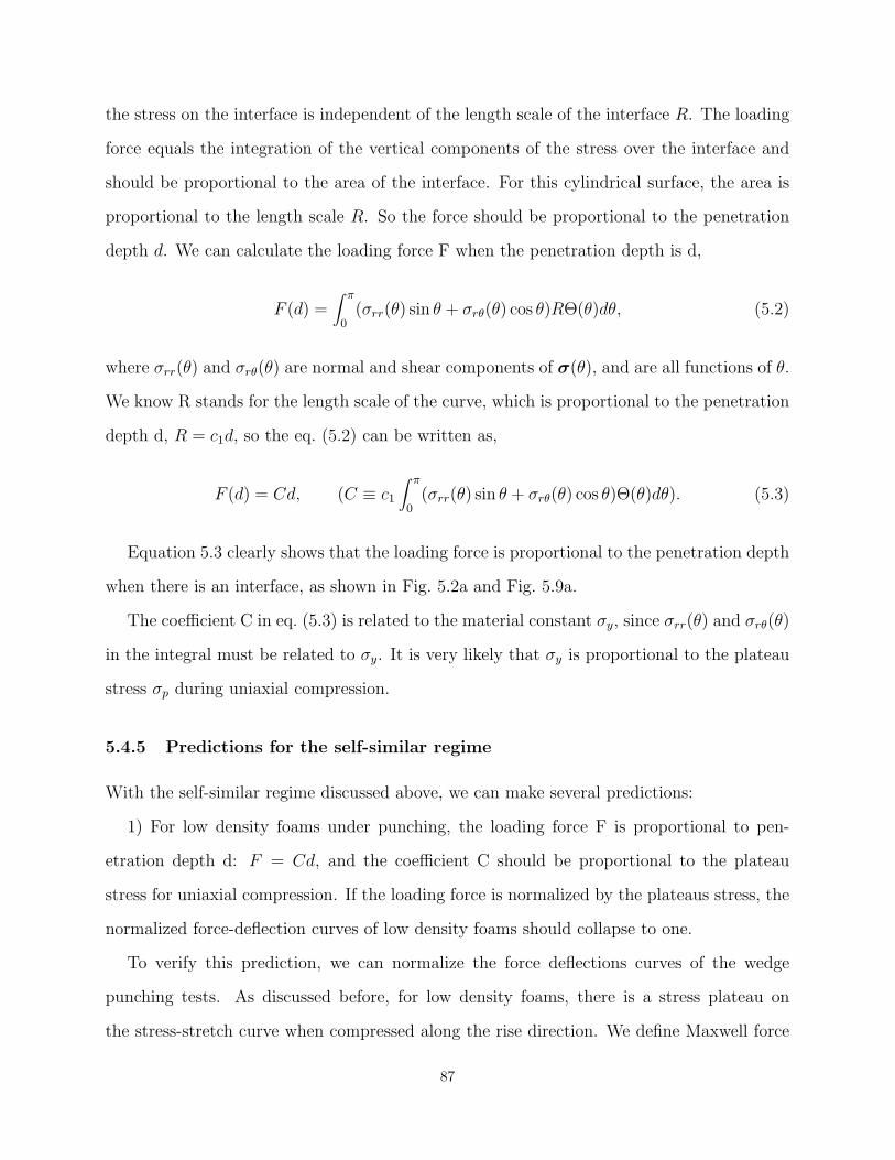
the stress on the interface is independent of the length scale of the interface R. The loading

force equals the integration of the vertical components of the stress over the interface and

should be proportional to the area of the interface. For this cylindrical surface, the area is

proportional to the length scale R. So the force should be proportional to the penetration

depth d. We can calculate the loading force F when the penetration depth is d,

F (d) =∫ π

0(σrr(θ) sin θ + σrθ(θ) cos θ)RΘ(θ)dθ, (5.2)

where σrr(θ) and σrθ(θ) are normal and shear components of σ(θ), and are all functions of θ.

We know R stands for the length scale of the curve, which is proportional to the penetration

depth d, R = c1d, so the eq. (5.2) can be written as,

F (d) = Cd, (C ≡ c1

∫ π

0(σrr(θ) sin θ + σrθ(θ) cos θ)Θ(θ)dθ). (5.3)

Equation 5.3 clearly shows that the loading force is proportional to the penetration depth

when there is an interface, as shown in Fig. 5.2a and Fig. 5.9a.

The coefficient C in eq. (5.3) is related to the material constant σy, since σrr(θ) and σrθ(θ)

in the integral must be related to σy. It is very likely that σy is proportional to the plateau

stress σp during uniaxial compression.

5.4.5 Predictions for the self-similar regime

With the self-similar regime discussed above, we can make several predictions:

1) For low density foams under punching, the loading force F is proportional to pen-

etration depth d: F = Cd, and the coefficient C should be proportional to the plateau

stress for uniaxial compression. If the loading force is normalized by the plateaus stress, the

normalized force-deflection curves of low density foams should collapse to one.

To verify this prediction, we can normalize the force deflections curves of the wedge

punching tests. As discussed before, for low density foams, there is a stress plateau on

the stress-stretch curve when compressed along the rise direction. We define Maxwell force

87

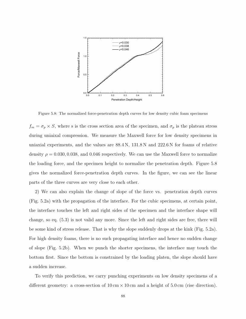
0.0 0.1 0.2 0.3 0.4 0.5 0.60.0

0.5

1.0

1.5

=0.030 =0.038 =0.046

Forc

e/M

axw

ell F

orce

Penetration Depth/Height

Figure 5.8: The normalized force-penetration depth curves for low density cubic foam specimens

fm = σp × S, where s is the cross section area of the specimen, and σp is the plateau stress

during uniaixal compression. We measure the Maxwell force for low density specimens in

uniaxial experiments, and the values are 88.4 N, 131.8 N and 222.6 N for foams of relative

density ρ = 0.030, 0.038, and 0.046 respectively. We can use the Maxwell force to normalize

the loading force, and the specimen height to normalize the penetration depth. Figure 5.8

gives the normalized force-penetration depth curves. In the figure, we can see the linear

parts of the three curves are very close to each other.

2) We can also explain the change of slope of the force vs. penetration depth curves

(Fig. 5.2a) with the propagation of the interface. For the cubic specimens, at certain point,

the interface touches the left and right sides of the specimen and the interface shape will

change, so eq. (5.3) is not valid any more. Since the left and right sides are free, there will

be some kind of stress release. That is why the slope suddenly drops at the kink (Fig. 5.2a).

For high density foams, there is no such propagating interface and hence no sudden change

of slope (Fig. 5.2b). When we punch the shorter specimens, the interface may touch the

bottom first. Since the bottom is constrained by the loading platen, the slope should have

a sudden increase.

To verify this prediction, we carry punching experiments on low density specimens of a

different geometry: a cross-section of 10 cm× 10 cm and a height of 5.0 cm (rise direction).

88

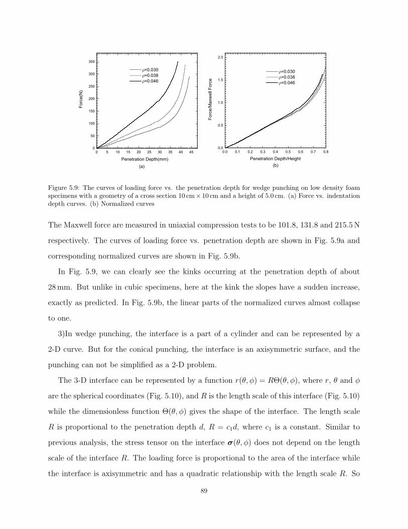
0 5 10 15 20 25 30 35 40 450

50

100

150

200

250

300

350

0.0 0.1 0.2 0.3 0.4 0.5 0.6 0.7 0.80.0

0.5

1.0

1.5

2.0

(b)

=0.030 =0.038 =0.046

Forc

e(N

)

Penetration Depth(mm)(a)

=0.030 =0.038 =0.046

Forc

e/M

axw

ell F

orce

Penetration Depth/Height

Figure 5.9: The curves of loading force vs. the penetration depth for wedge punching on low density foamspecimens with a geometry of a cross section 10 cm× 10 cm and a height of 5.0 cm. (a) Force vs. indentationdepth curves. (b) Normalized curves

The Maxwell force are measured in uniaxial compression tests to be 101.8, 131.8 and 215.5 N

respectively. The curves of loading force vs. penetration depth are shown in Fig. 5.9a and

corresponding normalized curves are shown in Fig. 5.9b.

In Fig. 5.9, we can clearly see the kinks occurring at the penetration depth of about

28 mm. But unlike in cubic specimens, here at the kink the slopes have a sudden increase,

exactly as predicted. In Fig. 5.9b, the linear parts of the normalized curves almost collapse

to one.

3)In wedge punching, the interface is a part of a cylinder and can be represented by a

2-D curve. But for the conical punching, the interface is an axisymmetric surface, and the

punching can not be simplified as a 2-D problem.

The 3-D interface can be represented by a function r(θ, φ) = RΘ(θ, φ), where r, θ and φ

are the spherical coordinates (Fig. 5.10), and R is the length scale of this interface (Fig. 5.10)

while the dimensionless function Θ(θ, φ) gives the shape of the interface. The length scale

R is proportional to the penetration depth d, R = c1d, where c1 is a constant. Similar to

previous analysis, the stress tensor on the interface σ(θ, φ) does not depend on the length

scale of the interface R. The loading force is proportional to the area of the interface while

the interface is axisymmetric and has a quadratic relationship with the length scale R. So

89

φ

Interface

(b)(a)

r

θ

Figure 5.10: (a) Conical punching experimental setting. (b) Sketch of the 3-D interface

we can expect the loading force has a quadratic relationship with the penetration depth d.

We can get the relationship between the loading force and the penetration depth

f(d) = Cd2, (C =∫ π

0

∫ 2π

0σ(θ, φ)n · e3Θ(θ, φ)dθdφ). (5.4)

In eq. (5.4), n is the normal of the surface and e3 is the vertical direction. This equation

predicts that the loading force is quadratic with penetration depth.

To verify this prediction, we carry punching tests with cone shaped punch, and details

are given in the following section.

5.5 Conical punching test

Using the same experimental setup with a cone punch of right angle, we performed conical

punching tests on low density foams (ρ = 0.030, 0.038, and 0.046). Both cubic specimens

and shorter specimens are tested. Fig. 5.10 gives the cone punching picture and the sketch

of the 3-D interface.

For the cubic specimens, the curves of loading force vs. penetration depth are shown

in Fig. 5.11a; corresponding normalized curves are shown in Fig. 5.11b (using the Maxwell

forces 88.4 N, 131.8 N and 222.6 N for specimens of density ρ = 0.030, 0.038, and 0.046

respectively).

90

0.0 0.1 0.2 0.3 0.4 0.5 0.6 0.7 0.80.0

0.2

0.4

0.6

0.8

1.0

1.2

1.4

1.6

1.8

0 10 20 30 40 50 60 70 80 900

100

200

300

400

(b)

=0.030 =0.038 =0.046

Load

ing

forc

e/M

axw

ell f

orce

Penetration Depth/Height

(a)

=0.030 =0.038 =0.046

Load

ing

forc

e(N

)

Penetration Depth (mm)

Figure 5.11: Conical punching on cubic specimens. (a) Loading force vs. penetration depth curves. (b)Corresponding normalized curves

0 10 20 30 40 500

100

200

300

400

0.0 0.1 0.2 0.3 0.4 0.5 0.6 0.7 0.8 0.90.0

0.5

1.0

1.5

2.0

2.5

(b)

Loa

ding

For

ce(N

)

=0.030 =0.038 =0.046

Penetration Depth(mm)(a)

=0.030 =0.038 =0.046

Load

ing

Forc

e/M

axw

ell F

orce

Penetration Depth/Height

Figure 5.12: Conical punching on shorter specimens. (a) Loading force vs. penetration depth curves. (b)Corresponding normalized curves

91

1 101

10

100

Loa

ding

For

ce(N

)

=0.030 =0.038 =0.046

Penetration Depth(mm)

y=0.1x22

1

Figure 5.13: Loading force vs. penetration depth curve in log-log space for conical punching on shortspecimens

Unlike wedge punching, there is no linear part in the curves, but there are still kinks.

The slope drop at the kinks shows the interface touches the free surface on the side. The

normalized curves are very close to each other, consistent with the first prediction.

For the shorter specimens (cross section 10 cm× 10 cm, height 5 cm), the curves of loading

force vs. penetration depth are shown in Fig. 5.12a; corresponding normalized curves are

shown in Fig. 5.12b (using the Maxwell forces 101.8 N, 131.8 N and 215.5 N for specimens

of density ρ = 0.030, 0.038 and 0.046 respectively). We can see kinks in Fig. 5.11. The

sudden slope jump at the kinks shows that the interface touches the bottom, consistent

with prediction 1. The normalized curves almost collapse to one curve, consistent with

prediction 2.

The initial parts in Fig. 5.11 and Fig. 5.12 look like parabola, in accord with eq. (5.4).

To be more accurate, we draw Fig. 5.12a in the log-log space. Fig. 5.13 clearly shows the

quadratic relationship between the loading force and penetration depth, exactly as eq. (5.4)

predicts.

92

5.6 Discussion

The surprising mechanical response observed in experiments with wedge-shaped and conical

punches may be traced to the behavior of the basic microstructural components of a polyether

polyurethane foam: the foam cells. Because the foam cells are bi-stable elastic structures,

the foam has two preferred values of strain, and the strain field consists of a high-strain

region and a low-strain region separated by a sharp interface. The strain jumps from one

preferred value of strain to the other preferred value of strain across the sharp interface.

As the penetration of the punch increases during an experiment, the preferred values of

strain do not change (since they are strictly properties of the foams); therefore, for the

strain field to accommodate the increasing penetration, the interface must expand. For lack

of a characteristic length other that the penetration, the sharp interface must expand in a

self-similar manner and in direct proportion to the penetration, in what we have termed the

self-similar regime. The geometrical simplicity of the self-similar regime makes the punching

experiments unexpectedly amenable to analytical treatment. The analysis indicates that

the mechanical response depends only on the dimensionality of the punch. For a two-

dimensional, wedge-shaped punch the response is linear whereas for a three-dimensional,

conical punch the response is quadratic. These straightforward predictions are in accord

with the experimental results.

93

Part II

Initial yielding of ultrathin films

94

Chapter 6

Surface stress and reversing size effectin the initial yielding of ultrathin films

6.1 Introduction

The mechanical behavior of tiny metallic bodies has long been known to be subject to size

effects (Bazant et al., 1997). For example, the yield stress of crystalline whiskers may exceed

the yield stress of large crystals of the same material by a factor of 10 or more (Brenner,

1956). With the development of nano technologies in recent years, much new research has

been devoted to elucidating size effects in polycrystalline ultrathin films.

One size effect that has drawn much attention pertains to the large strain gradients

that arise, for example, in films subjected to bending. This size effect has been ascribed

to the high density of geometrically necessary dislocations induced by the strain gradient

(Fleck et al., 1994, 1997). Another size effect pertains to the texture (or preferential grain

orientation) that is characteristic of thin films grown on crystalline substrates. Because a

texture frequently leads to a higher yield stress (Lejeck and Sima, 1983; Grant et al., 1988),

this size effect can be readily explained. Still another size effect pertains to the grain size,

which in annealed films tends to scale with the thickness of the film (Lejeck and Sima, 1983;

Grant et al., 1988). Because smaller grains lead to a higher yield stress, the so-called Hall–

Petch relation (Griffin et al., 1987; Venkatraman and Bravman, 1992; Thompson, 1993), or

perhaps to a lower yield stress, the reverse Hall–Petch relation, valid for grains smaller than

about 10 nm (Schiotz and Jacobsen, 2003), this size effect can be readily explained.

In a recent experimental study (Espinosa et al., 2004), the yield stress of gold films of

constant texture and grain size subjected to uniaxial applied tension showed a peculiar

size effect. The yield stress increased with diminishing film thickness, up to a thickness

95

h = 500 nm. Then, for h = 300 nm, the yield stress appeared to have remained the same

as for h = 500 nm, indicating that the yield stress had attained a maximum value for

h ≈ 400 nm. In another recent, similar experimental study (Saif, 2004), the yield stress of

pure aluminum films increased up to a thickness h = 100 nm; then, for h < 100 nm, the

yield stress started to decrease. This reversing (first hardening, then softening) size effect

cannot be explained by any of the models proposed so far, because those models predict a

hardening size effect (for constant grain size).

Here we model the film using continuum mechanics. We start by establishing expressions

for the compressive stresses induced in the film by the surface stress. After adding these

stresses to the applied stress, we use the von Mises yield condition to ascertain the value

of the applied stress at initial yielding or apparent yield stress . Our results indicate that in

films subjected to uniaxial applied tension the surface stress causes a reversing size effect on

the apparent tensile yield stress. Using the values of surface stress determined via atomistic

methods (Wan et al., 1999), we estimate that this size effect reverses for a thickness on the

order of 100 nm, in accord with the experimental results summarized above.

Then, we use the well-known failure criterion proposed Hancock and Mackenzie (1976)

to ascertain the mode of failure of the film. Our results indicate that the mode of failure

changes from ductile to brittle for thicknesses close to the thickness for which the size effect

reverses. These results are in accord with the experimental results of Espinosa et al. (2004).

Last, we show that the surface stress may lead to entirely disparate size effects depending

on the applied stress. In particular, we find that in films subjected to biaxial applied tension

the surface stress does not lead to a reversing size effect. This finding reconciles the recent

experimental results summarized above with J. W. Beams’s experiments on gold and silver

films, in which the size effect did not reverse even for h = 20 nm (Beams, 1959; Menter and

Pashley, 1959).

Our work joins a growing body of research in which the surface stress has been found to

play a crucial role in several problems at ultrasmall length scales, including the blunting of

a crack tip (Carlsson and Thomson, 1988) and the nanoindentation of a crystal (Knap and

96

Ortiz, 2003).

6.2 Surface stress

The surface stress is a second-rank tensor, Tαβ, where the indices α and β run from 1 to

2 and denote in-plane coordinates defined on the surface. (For detailed discussions of the

surface stress see, for example, Herring (1953); Cammarata (1994).) To relate the surface

stress to the surface energy, γ, using Eulerian coordinates (Nix and Gao, 1998), consider an

element of surface of area A that is stretched by an in-plane elastic strain εαβ. Then, the

work performed by the surface stress is dW = ATαβεαβ, and the energy of the element of

surface, γA, changes by d(γA) = γdA + Adγ = γAεµµ + A(∂γ/∂εαβ)εαβ, where repeated

indices imply summation. Equating dW to d(γA) results in the desired expression for the

surface stress, Tαβ = γδαβ + ∂γ/∂εαβ, where δαβ is the second-rank Kronecker delta. The

second term in the expression for Tαβ represents the change in surface energy associated

with the elastic stretching of the surface. When the area of a liquid surface is increased, the

surface does not stretch elastically, because the atoms in the interior of the liquid are mobile

and may readily migrate to the surface. Thus in liquids the second term in the expression

for Tαβ vanishes, and the surface stress is isotropic and equal to the surface energy. This is

not the case in solids, because in solids the long-range order in the positions of the atoms

makes it infeasible for the atoms to migrate to the surface, in particular when the strain

applied to the surface amounts to a displacement of a small fraction of the lattice constant.

Thus in solids the second term in the expression for Tαβ may not necessarily vanish, and the

surface stress is in general anisotropic.

Consider now the crystalline surface of a free-standing crystal. The surface accommodates

the lattice constant of the bulk of the material by means of a spontaneous elastic stretching.

If the crystalline surface possesses a threefold or higher rotational axial symmetry, then in

the expression for Tαβ the term ∂γ/∂εαβ associated with this elastic stretching is isotropic

(Wan et al., 1999). That is the case for (111) surfaces in FCC metals. In the experiments

97

2T/h

h

W

L

b

T

a

C1 C2 C1

hT

T

T

2T/h C2C1

Tdc

2T/h2T/h

e

2T/h

Figure 6.1: (a) A free-standing thin film. C1 and C2 are cuts performed for stress analysis. (b) The surfacestress T acting on the perimeter of C1. (c) The compressive stress induced by T on the surface of C1. (d)The compressive stress induced by T on the surface of C2. (e) Applied traction that gives the same stressesas T .

of interest here the films had a preferred 〈111〉 crystallographic texture normal to the faces

of the films, and we are justified in assuming an isotropic surface stress, Tαβ = Tδαβ. The

surface stress may in principle be either positive (tensile) or negative, but it is positive for

FCC metals.

6.3 The surface stress in thin films

Consider a free-standing film of length L À h and width W À h (Fig. 6.1a). Suppose

that the film is severed through its thickness along an arbitrary in-plane direction. (The cut

is marked C1 in Fig. 6.1a.) Then, the surface stress, which we assume to be positive and

isotropic, becomes manifest as a tensile force T per unit length of the perimeter of the cut,

acting normal to the surface of the cut, as indicated in Fig. 6.1b. If the severed parts of the

film are to remain in equilibrium, the surface stress must induce a compressive stress on the

98

surface of the cut; because the film is very thin, the induced stress is uniform and of value

−2T/h on the surface of the cut (Fig. 6.1c). Thus the surface stress induces a compressive

stress of value −2T/h in all in-plane directions (Herring, 1953).

Suppose now that the film is severed parallel to its upper and lower faces. (The cut is

marked C2 in Fig. 6.1a.) Then, the surface stress must again induce a compressive stress on

the surface of the cut, but now the stress is confined to a very narrow strip (of width ∼ h)

parallel to the lateral edges of the film, as indicated in Fig. 6.1d. Thus in most of the film

the surface stress induces no stress in the direction of the thickness of the film.

From our discussion so far, we conclude that in a film of thickness h the stresses induced

by the surface stress may be approximately simulated by (i) applying an in-plane compressive

traction of value −2T/h on all the lateral edges of the film and (ii) leaving the upper and

lower faces of the film traction-free (Fig. 6.1e). This conclusion is valid where the film is

thin, i.e., where L À h and W À h.

6.4 Apparent yield stress

Consider now a free-standing thin film to which a uniaxial stress σa is applied in the direction

of the length of the film. Then, the film is uniformly subjected to principal stresses σ1 =

σa − 2T/h, σ2 = −2T/h, and σ3 = 0 in the direction of the length, the width, and the

thickness, respectively. We may ascertain the value of the applied stress at initial yielding

or apparent yield stress , σya, by substituting the principal stresses in the von Mises yield

condition, 2σ2y = (σ1 − σ2)

2 +(σ2 − σ3)2 +(σ3 − σ1)

2, where σy is the yield stress (Calladine,

2000). The result is

σya

σy

=T

hσy

±√√√√1− 3

(T

hσy

)2

. (6.1)

Figure 6.2 shows a graphical rendition of (6.1) in the form of a plot of the dimensionless

apparent yield stress, σya/σy, vs. the dimensionless thickness, hσy/T . In the plot there is a

single curve separating the elastic region (which the curve embraces) from the plastic region.

The curve consists of two branches touching at their leftmost points (marked M in Fig. 6.2).

99

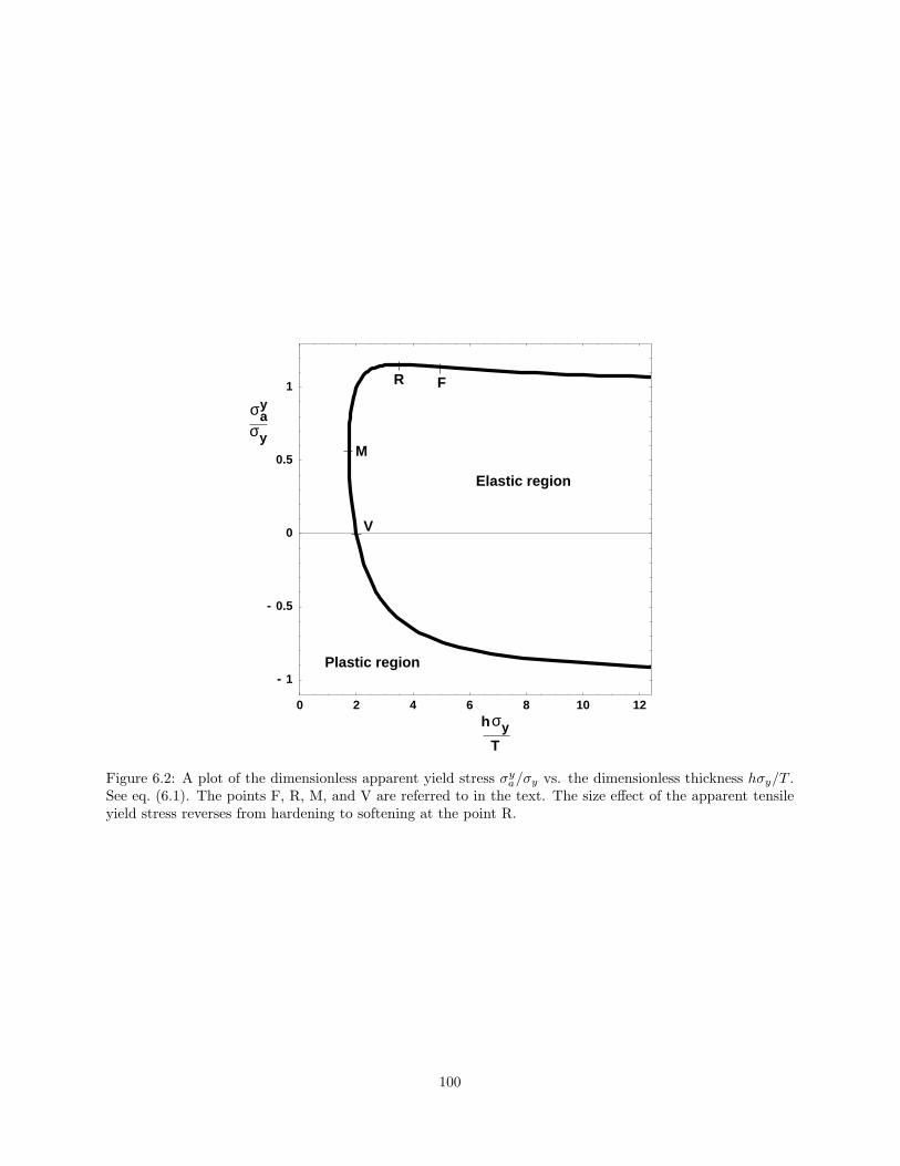
0 2 4 6 8 10 12

- 1

- 0.5

0

0.5

1

σ

y

ya

V

M

R F

yσh

Plastic region

σ

Elastic region

T

Figure 6.2: A plot of the dimensionless apparent yield stress σya/σy vs. the dimensionless thickness hσy/T .

See eq. (6.1). The points F, R, M, and V are referred to in the text. The size effect of the apparent tensileyield stress reverses from hardening to softening at the point R.

100

The upper branch corresponds to the + sign in (6.1) and gives the apparent tensile yield

stress. On the other hand, the lower branch corresponds to the − sign in (6.1) and gives

the apparent compressive yield stress. The branches are supported on h ≥ hM ≡ √3 T/σy

(because the discriminant of (6.1) is negative for h < hM). Therefore, a film of thickness

h < hM cannot be poised between the elastic region and the plastic region, regardless of the

applied stress; such a film is always in the plastic region.

Figure 6.2 indicates that for h À T/σy the apparent tensile yield stress is σy, and the

apparent compressive yield stress −σy. Thus for h À T/σy the initial yielding may be

attained by applying a tensile stress σy or a compressive stress −σy. This is the expected

asymptotic behavior.

Next, we discuss in turn the two branches of Fig. 6.2. Consider first the lower branch,

starting with a thin film of thickness h À T/σy. If the thickness of the film diminishes, the

absolute value of the apparent compressive yield stress decreases (i.e., d|σya|/dh < 0), and

we say that there is a softening size effect. If the thickness continues to diminish, then, for

a thickness h = hV ≡ 2 T/σy, the apparent compressive yield stress vanishes, σya = 0 (point

V in Fig. 6.2). Thus a free-standing film of thickness h = hV spontaneously attains the

initial yielding by virtue of the compressive stresses induced by the surface stress. When a

tensile stress is applied to this free-standing film, the film departs from the initial yielding,

enters the elastic region, and re-attains the initial yielding at the apparent tensile yield stress

given by the upper branch of Fig. 6.2. If the thickness continues to diminish beyond hV , the

apparent compressive yield stress becomes positive (i.e., the lower branch of Fig. 6.2 gives a

positive value of σya). This positive value of σy

a is the minimum tensile stress that must be

applied to the film if the film is not to yield by virtue of the compressive stresses induced

by the surface stress. (Therefore, the name “apparent compressive yield stress” remains

appropriate, even though this stress is positive.) Last, for a thickness h = hM ≡ √3 T/σy,

we reach the leftmost point of the lower branch.

Consider now the upper branch of Fig. 6.2, starting with a thin film of thickness h ÀT/σy. If the thickness of the film diminishes, the apparent tensile yield stress increases

101

(i.e., d|σya|/dh < 0), and we say that there is a hardening size effect. If the thickness of

the film continues to diminish, then, for a thickness h = hF ≈ 5 T/σy, the size effect is at

its most hardening (i.e., d2|σya|/dh2 = 0; point F in Fig. 6.2). If the thickness continues

to diminish beyond hF , then the hardening size effect starts to lessen (i.e., d|σya|/dh starts

to become less negative). Eventually, for a thickness h = hR ≡ 2√

3 T/σy ≈ 3.5 T/σy, the

apparent tensile yield stress attains its maximum value, σya = σy

aR ≡ 2σy/√

3 ≈ 1.15 σy, and

the size effect vanishes (i.e., d|σya|/dh = 0; point R in Fig. 6.2). If the thickness continues

to diminish beyond hR, the apparent tensile yield stress decreases (i.e., d|σya|/dh > 0),

and we say that there is a softening size effect. Thus for a thickness h = hV ≡ 2 T/σy

the apparent tensile yield stress equals its original value, σya = σy. Last, for a thickness

h = hM ≡ √3 T/σy ≈ 1.73 T/σy, the apparent tensile yield stress equals its minimum value,

σya = σy

aM ≡ σy/√

3 ≈ 0.58 σy, and we reach the leftmost point of the upper branch.

From our discussion of Fig. 6.2 we conclude that the surface stress causes a size effect on

the apparent tensile yield stress. For thin films of thickness h À T/σy there is a hardening

size effect, but the size effect reverses from hardening to softening for a thickness hR ≡2√

3 T/σy. Thus the stresses induced in a thin film by the surface stress lead to a size effect

of the type recently observed in experiments.

6.4.1 Size effects and the yield condition

We have predicated (6.1) on the von Mises yield condition, σe = σy. Here σe, the equivalent

stress , quantifies the forcing that tends to produce plastic deformation; it is defined by the

expression 2σ2e ≡ (σ1 − σ2)

2 +(σ2 − σ3)2 +(σ3 − σ1)

2, where σ1, σ2, and σ3 are the principal

stresses. This expression for σe suitably quantifies the forcing if the plastic deformation

occurs by the relative slip of adjacent planes in the material, regardless of the specific

mechanisms whereby the slip is effected. (The slip need not be effected by dislocation

motion, for example.) In fact, it is the yield stress, σy, and not the equivalent stress, σe,

that depends on the specific mechanisms whereby the slip is effected. Thus the elucidation

of size effects consists in determining the dependence of σy on the size. Yet this is not the

102

case for the size effect caused by the surface stress, because this size effect is unrelated to

the material. Instead, it is related to the stresses that act on the bulk of the material and

to the fact that these stresses differ from the applied stresses. The elucidation of this size

effect is not a problem in materials science, but rather a problem in solid mechanics.

In (6.1) the size effect caused by the surface stress is coupled to other size effects only

through the value of σy. Therefore, in (6.1) the yield stress σy is not the yield stress of the

bulk material, but the yield stress of the bulk material enhanced by any pertinent size effects

other than the size effect caused by the surface stress .

6.4.2 Comparison with experiments

In Section 6.4, we concluded that the size effect caused by the surface stress reverses from

hardening to softening for a thickness hR ≡ 2√

3 T/σy. To compare the predicted value of

hR with the experimental results, we recall that for h = hR the (maximum) apparent tensile

yield stress is σyaR ≡ 2σy/

√3, and write an expression for hR in terms of σy

aR, with the result

hR = 4T/σyaR.

(Note that σy = σyaR

√3/2 is the yield stress of the bulk material enhanced by any size

effects other than the size effect caused by the surface stress; see Section 6.4.1. Note also

that the expression hR = 4T/σyaR can give only a rough estimate of the thickness for which

the observed size effect reverses, not only because we have predicated this expression on a

number of simplifying assumptions, but also because (a) the value of T may be strongly

affected by subtle changes in environmental conditions and (b) σyaR is difficult to measure,

and tends to be overestimated both in experiments and in atomistic simulations; see, e.g.,

Schiotz et al. (1999).)

For the pure gold films of the experimental study of reference Espinosa et al. (2004), the

reported maximum apparent tensile yield stress was σyaR = 170 MPa. Using the surface stress

of gold given in reference (Wan et al., 1999), T = 3.41 N/m, we compute hR = 80 nm, which

is on the order of magnitude of the thickness for which the observed size effect reversed in

that study, h ≈ 400 nm.

103

For the pure aluminum thin films of the experimental study of Saif (2004), the reported

peak stress was σpa = 750 MPa, and we estimate σy

aR = σpa/2 = 375 MPa. Using the surface

stress of aluminum given in Wan et al. (1999), T = 2.29 N/m, we compute hR = 24 nm, which

is on the order of magnitude of the thickness for which the observed size effect reversed in

that study, h ≈ 100 nm.

6.4.3 A note on the values of the surface stress used in the comparison with

experiments

In the calculations above, we have use the (111) unrelaxed surface stress computed by

the modified embedded atom method and reported in Wan et al. (1999). (In this useful

reference, the surface stresses and surface energies obtained by a number of methods are

given for all FCC metals: Cu, Ag, Au, Ni, Pd, Pt, Al, and Pb. Different methods lead to

comparable results, and the results are in good agreement with the few available experimental

measurements.) Note that this surface stress corresponds to a free-standing crystal and does

not account for the additional elastic stretching undergone by the surface (as well as by the

bulk of the material) as the film is stressed to the initial yielding. The required correction

is negligible, however. In fact, a straightforward application of the atomistic model of Nix

and Gao (1998) allows us to estimate the required correction as ∆T ≈ 2Eεa, where E is the

Young’s modulus, ε is the strain associated with the additional elastic stretching, and a is

the lattice constant; for gold we use Eε = σy = 170 MPa and a = 0.3 nm, with the result

∆T ≈ 0.11 N/m ¿ T = 3.41 N/m.

Note also that a small increment in the plastic deformation brings additional atoms to

the surface of the film but does not cause an additional elastic stretching of the surface

(or of the bulk of the material) (Nix and Gao, 1998). We conclude that the area of the

surface of a film may change as a result of a small increment in plastic deformation, but the

surface retains the same structure and remains equally stretched, so that the energy of the

surface changes by TdA, where T is the surface stress of the free-standing film, and dA is

the change in surface area. As an example of application of this conclusion, consider a film

104

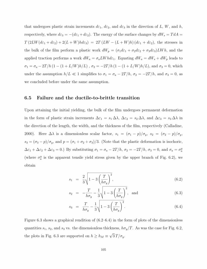
that undergoes plastic strain increments dε1, dε2, and dε3 in the direction of L, W , and h,

respectively, where dε3 = −(dε1 +dε2). The energy of the surface changes by dWs = TdA =

T (2LW (dε1 + dε2) + 2(L + W )hdε3) = 2T (LW − (L + W )h) (dε1 + dε2), the stresses in

the bulk of the film perform a plastic work dWp = (σ1dε1 + σ2dε2 + σ3dε3)LWh, and the

applied traction performs a work dWa = σaLWhdε1. Equating dWa = dWs + dWp leads to

σ1 = σa− 2T/h (1− (1 + L/W )h/L) , σ2 = −2T/h (1− (1 + L/W )h/L), and σ3 = 0, which

under the assumption h/L ¿ 1 simplifies to σ1 = σa − 2T/h, σ2 = −2T/h, and σ3 = 0, as

we concluded before under the same assumption.

6.5 Failure and the ductile-to-brittle transition

Upon attaining the initial yielding, the bulk of the film undergoes permanent deformation

in the form of plastic strain increments ∆ε1 = s1 ∆λ, ∆ε2 = s2 ∆λ, and ∆ε3 = s3 ∆λ in

the direction of the length, the width, and the thickness of the film, respectively (Calladine,

2000). Here ∆λ is a dimensionless scalar factor, s1 = (σ1 − p)/σy, s2 = (σ2 − p)/σy,

s3 = (σ3 − p)/σy, and p = (σ1 + σ2 + σ3)/3. (Note that the plastic deformation is isochoric,

∆ε1 + ∆ε2 + ∆ε3 = 0.) By substituting σ1 = σa − 2T/h, σ2 = −2T/h, σ3 = 0, and σa = σya

(where σya is the apparent tensile yield stress given by the upper branch of Fig. 6.2), we

obtain

s1 =2

3

√√√√1− 3

(T

hσy

)2

, (6.2)

s2 = − T

hσy

− 1

3

√√√√1− 3

(T

hσy

)2

, and (6.3)

s3 =T

hσy

− 1

3

√√√√1− 3

(T

hσy

)2

. (6.4)

Figure 6.3 shows a graphical rendition of (6.2–6.4) in the form of plots of the dimensionless

quantities s1, s2, and s3 vs. the dimensionless thickness, hσy/T . As was the case for Fig. 6.2,

the plots in Fig. 6.3 are supported on h ≥ hM ≡ √3 T/σy.

105

2 4 6 8 10 12

-0.6

-0.4

-0.2

0

0.2

0.4

0.6

yσh

s

s

1

3

2

s

s

T

Figure 6.3: A plot of the dimensionless quantities s1, s2, and s3 vs. the dimensionless thickness, hσy/T . Seeeqs. (6.2–6.4).

Consider now the process whereby the film accumulates plastic deformation, eventually

leading to failure in the form of fracture. According to a well-known failure criterion (Han-

cock and Mackenzie, 1976), the onset of failure occurs when the equivalent plastic strain, εe,

attains a critical value, εef , that depends on the triaxiality of the stress in the form

εef = ε0 exp (−p/σe), (6.5)

where the subscript “f” stands for “at failure,” ε0 is a dimensionless constant, p/σe is a

measure of the triaxiality of the stress, and the equivalent plastic strain is defined by the

expression 9 ε2e/2 = (∆ε1 − ∆ε2)

2 + (∆ε2 − ∆ε3)2 + (∆ε3 − ∆ε1)

2. By evaluating εe with

∆ε1 = s1 ∆λ, ∆ε2 = s2 ∆λ, ∆ε3 = s3 ∆λ, and the expressions for s1, s2, and s3 given by

(6.2–6.4), we obtain εe = 2 ∆λ/3; therefore, the value of ∆λ at failure is ∆λf = 3 εef/2. On

the other hand, by setting σe = σy and evaluating p with σ1 = σa − 2T/h, σ2 = −2T/h,

σ3 = 0, and σa = σya (where σy

a is the apparent tensile yield stress given by the upper branch

106

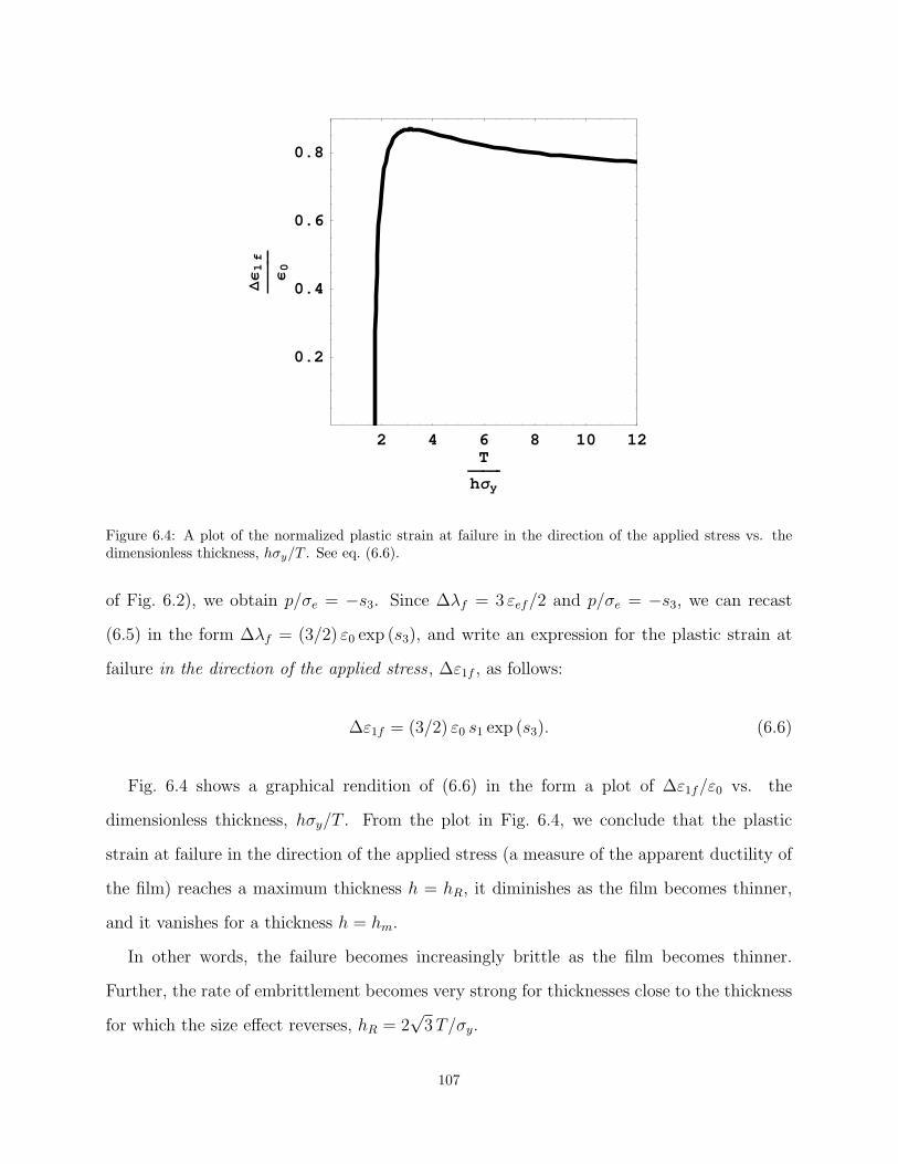
2 4 6 8 10 12T

���������

hΣy

0.2

0.4

0.6

0.8

DΕ1

f������������

Ε0

Figure 6.4: A plot of the normalized plastic strain at failure in the direction of the applied stress vs. thedimensionless thickness, hσy/T . See eq. (6.6).

of Fig. 6.2), we obtain p/σe = −s3. Since ∆λf = 3 εef/2 and p/σe = −s3, we can recast

(6.5) in the form ∆λf = (3/2) ε0 exp (s3), and write an expression for the plastic strain at

failure in the direction of the applied stress , ∆ε1f , as follows:

∆ε1f = (3/2) ε0 s1 exp (s3). (6.6)

Fig. 6.4 shows a graphical rendition of (6.6) in the form a plot of ∆ε1f/ε0 vs. the

dimensionless thickness, hσy/T . From the plot in Fig. 6.4, we conclude that the plastic

strain at failure in the direction of the applied stress (a measure of the apparent ductility of

the film) reaches a maximum thickness h = hR, it diminishes as the film becomes thinner,

and it vanishes for a thickness h = hm.

In other words, the failure becomes increasingly brittle as the film becomes thinner.

Further, the rate of embrittlement becomes very strong for thicknesses close to the thickness

for which the size effect reverses, hR = 2√

3 T/σy.

107

Our conclusions from the previous paragraph are in accord with the results of recent

experiments on gold films (Espinosa et al., 2004), in which a ductile-to-brittle transition was

documented for a thickness on the order of 100 nm.

6.6 Biaxial loading

To inquire further into the size effect caused by the surface stress, we now consider a type

of experiment known as the bulge test . In the bulge test, a film of thickness h is placed

across the open end of a circular tube of radius R À h. Then, the pressure of the air in

the tube is increased to a value p, whereupon the film deflects to form a bulge of height

b ¿ R. As a result, the film is subjected to a biaxial , in-plane isotropic applied stress

σa = pR2/4bh À p. In a classic experimental study, J. W. Beams used the bulge test to

determine the apparent yield stress of polycrystalline gold and silver films of thicknesses

in the range of 200 to 20 nm (Beams, 1959). He concluded that the apparent yield stress

increased monotonically with diminishing film thickness. Thus, in contrast with the recent

experimental studies summarized above, a reversing size effect was not observed in Beam’s

classical experimental study.

To understand this discrepancy, we substitute the principal stresses of the bulge test

(σ1 = σa − 2T/h, σ2 = σa − 2T/h, and σ3 = 0) in the von Mises yield condition, with the

result

σya

σy

= ±1 + 2T

hσy

, (6.7)

where σya is the apparent yield stress. It is straightforward to show that this same size effect

is valid for wires. For atomistic simulations in ultrathin wires, see, for example,Gall et al.

(2004). Equation (6.7) predicts a hardening size effect in the apparent tensile yield stress

measured in bulge tests, as expected. In a 1959 review paper (Menter and Pashley, 1959),

Beams is said to have first ascribed the hardening size effect observed in his experiments to

the surface energy. In the same paper, a plot is shown and attributed to Beams which might

be a graphical rendition of (6.7). Unfortunately, Beams appears not to have published the

108

equations leading to this plot. (He subsequently came to the conclusion that the size effect

observed in his experiments could not be ascribed to the surface energy, because for relatively

thick thin films the predicted size effect fell short of the observed size effect (Menter and

Pashley, 1959). It was thought at the time that the observed size effect should be ascribed

to a single reason.)

From our discussion of the bulge test we conclude that, in contrast with our results for

thin films subjected to a uniaxial applied stress, the surface stress does not lead to a reversing

size effect in thin films subjected to a biaxial, isotropic applied stress.

6.7 Discussion

Recent experiments (Espinosa et al., 2004) indicate that the yield stress of thin films of

constant texture and grain size subjected to uniaxial applied tension is subject to a peculiar

size effect. At first, the yield stress increases with diminishing film thickness. Then, the

yield stress is observed to attain a maximum value, whereupon a further decrease in the

thickness of the film leads to a decrease in the yield stress. In this chapter, we have been

concerned with this reversing (first hardening, then softening) size effect.

We have formulated a continuum model model which has allowed us to conclude that

in ultrathin, polycrystalline metallic films of constant grain size the surface stress leads to

a size effect in the initial yielding. This size effect depends strongly on the applied stress.

Where the applied stress is uniaxial, we have predicted that the size effect reverses for a

film thickness hR that can be estimated using values of the surface stress determined via

atomistic methods. The result, hR ≈ 100 nm, is in accord with experiments. In addition,

we have predicted that the mode of failure of the film changes from ductile to brittle for

thicknesses close to hR, also in accord with experiments.

Where the applied stress in biaxial, we have predicted a strong size effect, but the size

effect remains hardening for any film thickness, so that there should be no size-effect reversal.

This prediction is in accord with little-known but remarkable experiments performed 50 years

109

ago by J. W. Beams (Beams, 1959). In these biaxial experiments with gold and silver films,

the size effect did not reverse even for a film thickness as low as 20 nm.

Our work joins a body of research in which the surface stress has been found to play a

crucial role in several problems at ultrasmall length scales, including the blunting of a crack

tip (Carlsson and Thomson, 1988) and the nanoindentation of a crystal (Knap and Ortiz,

2003). Given that the film thickness for which the size effect reverses is only about 100 times

a typical lattice parameter, our conclusions add to a growing realization of the robustness

of continuum mechanics at ultra-small length scales, a realization that has been commented

upon by a number of authors (for a recent, eloquent example from the field of microfluidics,

see Sharp and Adrian (2004)).

110

Chapter 7

Summary and conclusions

In the first part of this work, we have studied the mechanical behavior of elastic polyether

polyurethane (EPP) foams by means of experiments, theory, and models. We designed our

experiments with four observations in mind.

1. In most engineering applications of EPP foams, the foams are subjected to multiaxial

loading, yet there has been scant research on the mechanical response of EPP foams

under multiaxial states of stress.

2. The mechanical response of an EPP foam depends not just quantitatively but also

qualitatively on the relative density of the foam, yet no experiments have been reported

for a series of EPP foams of widely differing densities.

3. EPP foams are commonly subjected to large strains under service conditions, yet there

have been few measurements of complete stress-strain curves, and these measurements

have been mostly limited to uniaxial tests.

4. In tests in which the stress field is spatially homogeneous, a stress plateau is a frequent

occurrence and appears to be invariably accompanied by heterogeneous strain fields,

yet measurements of the strain fields have only been performed in a few uniaxial tests.

We have conducted an unprecedented set of experiments on a commercial series of EPP

foams. This commercial series of EPP foams consists of five different foams covering the

entire range of densities commonly used in applications. We have tested each foam under

five different loading cases including uniaxial, biaxial, and triaxial loading cases. In each test

we have measured a complete stress–strain curve up to large strains on the order of 50%.

111

For several tests we have also used a global digital image correlation method to ascertain

the nature of the strain fields.

Consistent with earlier experimental results, we have found that EPP foams can be clas-

sified into low-density foams and high-density foams on the basis of the stress-strain curves

measured under uniaxial compression along the rise direction. The stress-strain curves of

low-density foams exhibit a stress plateau whereas the stress-strain curves of high-density

foams harden monotonically. Among the foams of our experiments, we have found the three

foams of lower density to be low-density foams.

We have determined that the classification of foams into low-density foams and high-

density foams holds consistently for all loading cases. The same three foams of lower density,

and then only those three foams, gave a stress plateau under every loading case in which

stress plateaus were observed.

We have confirmed that a stress plateau in the mechanical response of a low-density foam

is invariably accompanied by heterogeneous strain fields. These heterogeneous strain fields

display two preferred values of strain; an increase in the applied mean strain is accommodated

by growth of the volume fraction of one of the preferred values of strain at the expense of

the volume fraction of other preferred value of strain.

Our experimental findings are inconsistent with currently available models of elastic

foams. In these models, the microstructure of a foam undergoes a bifurcation of equilib-

rium (Euler buckling); the plateau stress corresponds to an eigenvalue; and the attendant

strain field corresponds to an eigenfunction of arbitrary amplitude. As the applied mean

strain is increased following buckling, the stress-strain curve traces a stress plateau. The

strain field remains invariant except for its amplitude, which increases to accommodate the

applied mean strain. But a strain field that remains invariant except for its amplitude can-

not be reconciled with the experiments, where the strain fields display two fixed, preferred

values of strain, and an increase in the applied mean strain is accommodated by growth of

the volume fraction of one of the preferred values of strain at the expense of the volume

fraction of other preferred value of strain.

112

We have argued that the conjunction of stress plateaus and strain fields with two preferred

values of strain indicates that at large strains the deformation of EPP foams is dominated

by a phase transition. Thus we have ascribed the preferred values of strain observed in ex-

periments to two configurational phases of the foam, and identified the strain fields observed

in experiments and the attendant plateau stress with two-phase strain fields and a Maxwell

stress, respectively.

We have formulated a 3D model of EPP foams. In this model, a unit cell composed of

several bars is cut off from an idealized, perfectly periodic foam microstructure. The tips of

the bars of the unit cell are subjected to a set of displacements affine with the applied mean

deformation gradient, and left to rotate freely. This is, therefore, a mean-field model.

The unit cell is characterized using a few physically meaningful material and geometric

parameters whose values may be readily estimated for any given foam. As we have been

mostly interested in the mechanical response at large strains, we have adopted for the sake

of simplicity a linear elastic model for the polyether polyurethane.

We have verified that for uniaxial compressive loading along the rise direction the model

predicts configurational phase transitions, stress plateaus, and two-phase strain fields for

low-density foams; a critical point for foams of critical density; and monotonically harden-

ing stress-strain curves and homogeneous strain fields for high-density foams. The critical

exponents associated with the critical point are the same as in other mean-field models such

as the Van der Walls model of a fluid. These predictions are consistent with, and provide a

straightforward theoretical interpretation to, the experimental results.

From an analysis of the model, we have concluded that the mechanical response of EPP

foams is dominated at large strains by either one of two mechanisms.

1. Snap-through buckling of a foam cell, a mechanism that entails nonconvex strain energy

functions, stress plateaus, and two-phase strain fields. Snap-through buckling represents

the attainment of a limit point. In contrast to Euler buckling, a global mechanism in

which the entire microstructure of a foam is engaged at once, snap-through buckling is

113

a local mechanism that sweeps progressively through the microstructure of the foam.

Here a foam cell is slender and undergoes a discontinuous transition between two char-

acteristic configurational phases, without bifurcation of equilibrium.

2. Bending of a foam cell, a mechanism that entails convex strain energy functions, mono-

tonically increasing stresses, and homogeneous strain fields. Here a foam cell is thickset

and deforms continuously and in concert with all the other cells.

We have calibrated the model and shown that with a suitable choice of parameters, the

model gives predictions in good accord with all our experiments.

To the best of our knowledge, we are the first to have compared experimental and pre-

dicted stress-strain curves for numerous loading cases and a complete series of foams of

widely differing densities. We have shown that the model is capable of reproducing all the

trends evinced in the experimental stress-strain curves. Further, even though we have not

made a special effort at curve fitting, the model gives good fits for all loading cases with the

exception of the triaxial loading case, where the fits can be said to be reasonable.

We have noted, however, that the goodness of a model of EPP foams cannot consist

in the capacity of the model to give close fits to numerous stress-strain curves measured

in experiments. The model should be able to account for all the relevant experimental

evidence, and our experiments indicate that in EPP foams the character of a stress-strain

curve is closely linked to the character of the attendant strain fields, which have hardly been

the subject of any research.

Thus, in judging the performance of our model, we have highlighted the capacity of the

model to give a nonconvex strain energy function—the signature of a phase transition, which

entails the conjunction of a stress plateau and two-phase strain fields—where and only where

our experiments evinced a stress plateau and two-phase strain fields. We have submitted

that this should remain a fundamental criterion of goodness in the evaluation of constitutive

models of EPP foams.

114

We have performed an extensive experimental and theoretical study of punching in EPP

foams. The motivation for this study has been the fact that EPP foams are widely used in

packaging, helmets, car seats, sandwich panels, and other applications where an EPP foam

is subjected to punching.

In experiments in which a low-density EPP foam specimen was penetrated with a wedge-

shaped punch, we have found that the force–penetration curve remained linear up to a

penetration of the punch of about 40% of the height of the specimen. Then, as the pene-

tration proceeded, the mechanical response became nonlinear and might evince an abrupt

lessening or increase in stiffness, depending on the aspect ratio of the specimen.

To explain these surprising experimental results, we have proposed that in a foam speci-

men subjected to punching the strain field consists of a high-strain phase in a region close to

the tip, where a phase transition has already taken place, and a low-strain phase in a region

far from the tip, where the phase transition is yet to take place. The two configurational

phases must be separated by a sharp interface, and we have used a global DIC method to

trace the sharp interface as it grew and swept through a specimen during a test.

By studying theoretically the self-similar growth of the sharp interface between the two

configurational phases of a foam, we have predicted a linear response within the self-similar

regime, in accord with the experimental observations. We have also shown that the force-

penetration curves for foams of different densities can be made to collapse onto a single curve

within the self-similar regime, provided that each individual curve is scaled by the plateau

stress of the corresponding foam.

We have argued that the self-similar regime ends when the sharp interface reaches one

of the boundaries of the specimen. Depending on the aspect ratio of the specimen, the

sharp interface will first reach either a lateral boundary or the lower boundary. If a lateral,

unsupported boundary is reached first, the mechanical response will display a momentary

loss of stiffness. If the lower, fixed boundary is reached first, the mechanical response will

display a sizable increase in stiffness. We have shown these predictions to be in accord with

our experimental results.

115

By applying the same theory to the case of a conical punch, we have predicted a quadratic

response within the self-similar regime and verified our prediction by performing experiments

with a conical punch.

We have concluded that in the self-similar regime the mechanical response is ruled entirely

by geometry, and depends only on the dimensionality of the punch and the plateau stress of

the low-density foam. Thus the self-similar regime is a direct manifestation of the occurrence

of a phase transition.

In the second part of this thesis, we have undertaken a theoretical study of the initial

yielding of ultrathin metallic films. It has recently been found that in free-standing metallic

films of constant grain size the initial yield stress increases as the film becomes thinner, it

peaks for a thickness on the order of 100 nm, and then starts to decrease. This reversing (first

hardening, then softening) size effect has posed two challenges: (1) It cannot be explained

using currently available models and (2) it appears to contradict the classical experimental

results of J. W. Beams [1959], in which the size effect in bulge tests did not reverse even for

a thickness of 20 nm.

We have shown that the reversing size effect can be explained and the contradiction

dispelled by taking into account the effect of the surface stress on the initial yielding. We

have used a simple continuum model to predict that the mode of failure of a film changes

from ductile to brittle for a thickness on the order of 100 nm, in accord with experimental

measurements.

We have concluded that our successful application of methods of continuum mechanics

to films as thin as 100 times a typical lattice parameter adds to a growing realization of the

robustness of these methods at ultrasmall length scales.

116

References

Artavia L. D. and Macosko C. W., 1994, “Polyurethane flexible foam formation,” in Low density cellular plastics:Physical basis of behavior , edited by Hilyard N. C. and Cunningham A. (Chapman and Hall, London), pp. 22–55.

Bart-Smith, H., Bastawros, A. F., Mumm, D. R., Evans, A. G., Sypeck, D. J., Wadley, H. N. G., 1998, “Compressivedeformation and yielding mechanisms in cellular Al alloys determined using X-ray tomography and surface strainmapping,” Acta. Mater., 46, pp. 3583–3592.

Bastawros, A. F., Bart-Smith, H., Evans, A. G., 2000, “Experimental analysis of deformation mechanisms in aclosed-cell aluminum alloy foam,” J. Mech. Phys. Solids, 48, pp. 301–322.

Bayer, O., 1947, “Das di-isocyanat-polyadditionsverfahren (polyurethane),” Angewandte Chemie, 59, pp. 257–272.

Bazant, Z. P., and Chen, E. P., 1997, “Scaling of Structural Failure,” Appl. Mech. Reviews, 10, pp. 593–527.

Beams, J. W., 1959, “Mechanical Properties of Thin Films of Gold and Silver,” in Structure and Properties of ThinFilms, edited by Neugebauer, C. A., Newkirk, C. A., and Vermilyea, D. A. (John Willey & Sons, New York), pp.183–198.

Berfield T. A., Patel J. K., Shimmin R. G., Braun P. V., Lambros J., and Sottos N. R., 2006, “Fluorescent ImageCorrelation for Nanoscale Deformation Measurements,” Small 2, pp. 631–635.

Borodich F. M., 1983, “Similarity in the problem of contact between elastic bodies,” J. Appl. Math. Mech., 47, pp.519–521.

Borodich F. M., 1989, “Hertz contact problems for an anisotropic physically nonlinear elastic medium,” Strength.Mater., 12, pp. 1668–1676.

Brakke K., “The surface evolver,” Experimental Mathematics, 1, pp. 141–165.

Brenner, S. S., 1956, “Tensile Strength of Whiskers,” J. Applied Phys., 27, pp. 1484–1491.

Brydona A. D., Bardenhagena S. G., Millerb E. A., and Seidlerb G. T., 2005, “Simulation of the densification of realopen-celled foam microstructures,” J. Mech. Phys. Solids, 53, pp. 2638–2660.

Cammarata, R. C., 1994, “Surface and Interface Stress Effects in Thin-Films,” Prog. Surf. Sci., 46, pp. 1–38.

Calladine, C. R., Plasticity (Horwood Publishing Ltd., Chichester, UK, 2000), p. 48.

Cao, Y., Bly, R., Moore, W., Gao, Z., Cuitino, A. M., Soboyejo, W. O., 2006, “Investigation of viscoelasticity ofhuman osteosarcoma cells using shear assay experiments,” J. Mater. Res., 21, pp. 1922–1930.

Cao, Y., Bly R., Moore W., Gao Z., Cuitino A. M., Soboyejo W. O., 2007, “On the measurement of human osteosar-coma cell elastic modulus using shear assay experiments,” J. Mater. Sci. Mater. Med., 18, pp. 103–109.

Carlsson, A. E. and Thomson, R., 1988, “Fracture Toughness of Materials: From Atomistics to Continuum Theory,”Solid State Phys., 51, pp. 233–280.

Cardenas-Garcia, J. F., Yao, H., Zheng, S., Zartman, R. E., 1998, “Digital image correlation procedure to characterizesoil surface layer cracking,” Agronomy J., 90, pp. 438–441.

Chao, Y. J., Luo, P. F., Kalthoff, J. F., 1998, “An experimental study of the deformation fields around a propagatingcrack tip,” Exp. Mech., 38, pp. 79–85.

117

Chen, C., Lu, T. J. and Fleck, N. A., 1999, “Effect of imperfections on the yielding of two-dimensional foams,” J.Mech. Phys. Solids, 47, pp. 2235–2272.

Chung, J. and Waas, A. M., 2002, “Compressive response of circular cell polycarbonate honeycombs under inplanebiaxial static and dynamic loading. Part I: experiments,” Int. J. Impact Eng., 27, pp. 729–754.

Chung, J. and Waas, A. M., 2002, “Compressive response of circular cell polycarbonate honeycombs under inplanebiaxial static and dynamic loading - Part II: simulations,” Int. J. Impact Eng., 27, pp. 1015–1047.

Coniglio, A., Fierro, A., Nicodemi M., Pica Ciamarra M. and Tarzia M. , 2005, “Statistical mechanics of densegranular media,” J. Phys. Condens. Matter, 17, pp. 2557–2572.

Dai, X., and Gioia, G., 2008, “Critical exponents in elastic foams,” Proceedings of the 10th Pan American Congressof Applied Mechanics (PACAM X), pp. 331–334.

Daxner, T., 2003, Multi-Scale modeling and simulation of metallic foams, PhD thesis, by VDI Verlag

Deshpande, V. S. and Fleck, N. A., 2001, “Multi-axial Yield Behaviour of Polymer Foams,” Acta mater., 49, pp.1859–1866.

Espinosa, H. D., Prorok, B. C., and Peng, B., 2004, “Plasticity Size Effects in Free-Standing Submicron PolycrystallineFCC Films Subjected to Pure Tension,” J. Mech. Phys. Solids, 52, pp. 667–689.

Fleck, N. A., Muller, G. M., Ashby, M. F., Hutchinson, J. W., 1994, “Strain Gradient Plasticity: Theory andExperiment,” Acta Metall. Mater., 42, pp. 475–487.

Fleck, N. A., and Hutchinson, J. W., 1997, “Strain Gradient Plasticity,” Adv. Appl. Mech., 33, pp. 295–261.

Galanov, B. A., 1981, “Approximate solution to some problems of elastic contact of two bodies,” Mech. Solids, 16pp. 61–67.

Gall, K., Diao, J., and Dunn, M. L., 2004, “The Strength of Gold Nanowires,” Nanoletters, 4, pp. 2431–2436.

Gao, Z., Wang, Y., Gioia, G., and Cuitino, A. M. 2002, “A Global Approach for Digital Speckle Correlation,”Proceedings of the 2002 SEM Annual Conference & Exposition on Experimental and Applied Mechanics, Societyfor Experimental Mechanics, pp. 250–254.

Gao, Z. and Desai, J. P., 2009, “Estimating zero-strain states of very soft tissue under gravity loading using digitalimage correlation,” Med. Image Anal., 14, pp. 126–137.

Gdoutos E. E., Daniel I. M. and Wang K. A., 2002, “Failure of Cellular Foams under Multiaxial Loading,” Compos.A: Appl. Sci. Manuf., 33, pp. 163–176.

Gent, A. N., Thomas, A. G., 1963, “Mechanics of foamed elastic materials,” Rubber Chem. Tech., 36, pp. 597–610.

Gibson L. J., Ashby M. F., Schajer, G. S. and Robertson, C. I., 1982, “The mechanics of two-dimensional cellularmaterials,” Proc. R. Soc. Lond, A382, pp. 25–42.

Gibson L. J and Ashby M. F., 1982, “The mechanics of three-dimensional cellular materials,” Proc. R. Soc. Lond,A382, pp. 43–59.

Gibson, L. J. and Ashby, M. F., 1997, Cellular Solids: Structure and Properties, 2nd ed. Cambridge University Press,UK

Gioia, G., Wang, Y. and Cuitino, A. M., 2001, “The energetics of heterogeneous deformation in open-cell solid foams,”Proc. R. Soc. Lond. A, 457, pp. 1079–1096.

Global Industry Analyst, Inc., 2008 “Polymeric foams: a global strategic business report”, CODE: MCP-1174

Goldenfeld, N., 1992, Lectures on Phase Transition and the Renormalization Group (Frontiers in Physics, 85), byWestview Press.

Gong, L., Kyrikides, S., and Jang W. Y., 2005, “Compressive response of open-cell foams, part i: Morphology andelastic properties,” Int. J. Solid. Struct., 42, pp. 1355–1379.

118

Gong, L., and Kyriakides, S., 2005, “Compressive response of open cell foams, Part II: Initiation and evolution ofcrushing,” Int. J. Solid. Struct., 42, pp. 1381–1399.

Gong, L., 2005, The compressive response of open-cell foams, PhD thesis, The University of Texas at Austin

Grant, E. M., Hansen, N., Jensen, D. J., Ralph, B., Stobbs, W. M., 1988, “Texture Development During GrainGrowth in Thin Films,” in Proceedings of the Eighth International Conference on Texture of Materials , edited byKallend, J. S., and Gottstein, G. (Springer-Verlag, New York ).

Griffin, A. J., Brotzen, F. R., and Dunn, C. F., 1987, “Mechanical-Properties and Microstructures of Al-1-Percent-SiThin-Film Metallizations,” Thin Solid Films, 150, pp. 237–244.

Hancock, J. W., and Mackenzie, A. C., 1976, “On the Mechanisms of Ductile Failure in High-Strength Steels Subjectedto Multi-Axial Stress States,” J. Mech. Phys. Solids, 24, pp. 147–169.

He, Z. H., Sutton, M. A., Ranson, W. F., and Peters, W. H., 1984, “Two-dimensional fluid-velocity measurementsby use of digital-speckle correlation techniques,” Exp. Mech., 24, pp. 117–121.

Herring, C., 1953, in Structure and Properties of Solid Surfaces , edited by Gomer, R. and Smith, C. S. (The Universityof Chicago Press).

Jang W. Y., Kraynik A. M., and Kyriakides S., 2008, “On the microstructure of open-cell foams and its effect onelastic properties,” Int. J. Solid. Struct., 45, pp. 1845–1875.

Knap, J. and Ortiz, M., 2003, “Effect of Indenter-Radius Size on Au(001) Nanoindentation,” Phys. Rev. Lett., 90,226102.

Lakes, R., Rosakis, P., and Ruina A., 1993, “Microbuckling Instability in Elastomeric Cellular Solids,” J. Mater. Sci.28, pp. 667–4672.

Laroussi M., Sab A., and Alaoui A., 2002, “Foam mechanics: nonlinear response of an elastic 3D-periodic microstruc-ture,” Int. J. Solid. Struct., 39, pp. 3599–3623.

Lejeck P., and Sima, V., 1983, “Orientational Relationships in the Secondary Recrystallization of Pure Nickel,”Mater. Sci. Eng., 60, pp. 121–124.

Lockwood, W. D. and Reynolds, A. P., 1999, “Use and verification of digital image correlation for automated 3-Dsurface characterization in the scanning electron microscope,” Mater. Characterization, 42, pp. 123–134.

Lu, H., 1998, “Applications of digital speckle correlation to microscopic strain measurement and materials propertycharacterization,” J. Electron. Packag., 120, pp. 275–279.

Maire E., Fazekasb A., Salvob L., Dendievelb R., Youssefa S., Cloetensc P. and Letangd J. M., 2003, “X-ray tomog-raphy applied to the characterization of cellular materials Related finite element modeling problems,” Compos.Sci. Tech., 63, pp. 2431–2443.

Ma, l., Zhou, J. et al, 2002, “Self-similarity simplification approaches for the modeling and anlysis of Rockwellhardness indentation,” J. Res. Natl. Inst. Stand. Technol., 107, pp. 401–412.

Magnenet, V., Rahouadj R., Bacher P., and Cunat C., 2008, “Inelastic constitutive relations for foamed materials:A statistical approach and its application to open-cell melamine,” Mech. Mater., 40, pp. 673–684.

Mehta A and Edwards S. F., 1989, “Statistical mechanics of powder mixtures,” Physica A, 157, pp. 1091–1097.

Maji A. k, Schreyer H. l, Donald S, Zuo Q and Satpathi D, 1995, “Mechanical Properties of Polyurethane FoamImpact Limiters,” J. Eng. Mech., 121, pp. 528–540.

Makse, H. A. and Kurchan J., 2002, “Testing the thermodynamic approach to granular matter with a numericalmodel of a decisive experiment,” Nature, 415, pp. 614–616.

Menges G., Knipschild F., 1975, “Estimation of mechanical-properties for rigid polyurethane foams,” Polymer Eng.Sci., 15, pp. 623–627

119

Menter, J. W. and Pashley, D. W., 1959, “The Microstructure and Mechanical Properties of Thin Films,” in Structureand Properties of Thin Films , edited by Neugebauer, C. A., Newkirk, C. A., and Vermilyea, D. A. (John Willey& Sons, New York), pp. 111–150.

MILLS, N. J., 1997, “Time dependence of the compressive response of polypropylene bead foam,” CELLULARPOLYMERS, 16, pp. 194–215.

MILLS, N. J., FITZGERALD, C., GILCHRIST, A. and VERDEJO R, 2003, “Polymer foams for personal protection:cushions, shoes and helmets,” Compos. Sci. Tech., 63, pp. 2389–2400.

Mizuno, Y., Kawasaki, A. and Watanabe, R., 1995, “In situ measurement of sintering shrinkage in powder compactsby digital image correlation method,” Powder Metallurgy, 38, pp. 191–195.

Mohr, D. and Doyoyo, M. A., 2003, “New Method for the Biaxial Testing of Cellular Solids,” Exp. Mech., 43, pp.173–182.

Mullins L., 1969, “Softening of rubber by deformation,” Rub. Chem. Technol., 42, pp. 339–362.

Myriam L., Karam S. and Amina A., 2002, “Foam mechanics: nonlinear response of an elastic 3D-Peiodicmicrostructure,” Int. J. Solid. Struct., 39, pp. 3599–3623.

Nix, W. D. and Gao, H., 1998, “An Atomistic Interpretation of Interface Stress,” Scripta Mater., 39, pp. 1653–1661.

Okumura D., Ohno N. and Noguchi H., 2004, “Elastoplastic microscopic bifurcation and post-bifurcation behaviorof periodic cellular solids,” J. Mech. Phys. Solids, 52, pp. 641–666.

Overaker D. W., Cuitino A. M. and Langrana N. A., 1998, “Elastoplastic micromechanical modeling of two-dimensional irregular convex and nonconvex (re-entrant) hexagonal foams,” Trans. ASME J. Appl. Mech., 65,pp. 748–757.

Papka S. D. and Kyriakides S., 1994, “In-plane compressive response and crushing of honeycomb,” J. Mech. Phys.Solids, 42, pp. 1499–1532.

Papka, S. D. and Kyriakides, S., 1999, “Biaxial crushing of honeycombs - Part I: Experiments,” Int. J. Solid. Struct.,36, pp. 4367–4396.

Papka, S. D. and Kyriakides, S., 1999, “In-plane biaxial crushing of honeycombs - Part II: Analysis,” Int. J. Solid.Struct., 36, pp. 4397–4423.

Patel N. R. and Finnie I., 1970, “Structural features and mechanical properties of rigid cellular plastics,” J. Mater.,5, pp. 909–932.

Plateau J. A. F., 1873, Statique Experimentale et Theorique des Liquides soumis aux Seules Forces Moleculaires,(Gauthier-Villars, Paris) .

Reyes, A., Hopperstad, O. S., Berstad, T., Hanssen, A. G. and Langseth, M., 2003, “Constitutive modeling ofaluminum foam including fracture and statistical variation of density,” Eur. J. Mech. A Solids, 22, pp. 815–835.

Sabuwala T., Dai X., and Gioia G., Large Deformation Behavior of Low Density Open Cell Foams. 2007 ASMEApplied Mechanics and Materials Conference, Austin, Texas

Saif, T., 2004, “Scaling the Depths,” Mech. Engr., 126, pp. 8–11. See also Haque, A., 2002, “Length-Scale Effectson Nano-Scale Materials Behavior,” PhD Thesis, Department of Mechanical Engineering, University of Illinois atUrbana-Champaign.

Schiotz, J., Vegge, T., Di Tolla, F. D., and Jacobsen, K. W., 1999, “Atomic-scale Simulations of the MechanicalDeformation on Nanocrystalline Metals,” Phys. Rev. B, 60, pp. 11971–11983.

Schiotz, J. and Jacobsen, K. W., 2003, “A Maximum in the Strength of Nanocrystalline Copper,” Science, 301, pp.1357–1359.

Schraad M. W., and Harlow F. H., 2006, “A stochastic constitutive model for disordered cellular materials: Finite-strain uni-axial compression,” Int. J. Solid. Struct., 43, pp. 3542–3568.

120

Sharp, K. V., and Adrian R. J., 2004, “Transition from Laminar to Turbulent Flow in Liquid Filled Microtubes,”Exp. Fluids, 36, pp. 741–747.

Shaw, M. C., and Sata, T., 1966, “The Plastic Behavior of Cellular Materials,” Int. J. Mech. Sci., 8, pp. 469–478.

Sudheer Kumar, P., Ramachandra S. and Ramamurty U., 2003, “Effect of displacement-rate on the indentationbehavior of an aluminum foam,” Mater. Sci. Eng. A, 347, pp. 330–337.

Sullivan R. M., Ghosn L. J. and Lerch B. A., 2008, “A general tetrakaidecahedron model for open-celled foams,” Int.J. Solid. Struct., 45, pp. 1754–1765.

Timoshenko, S. P., 1956, Strength of Materials; Part III, Advanced Theory and Problems, (D. Van Nostrand Co.,Princeton, New Jersey, Third Edition edition)

Thompson, W. (Lord Kelvin), 1887, “On the division of space with minimal partitional area,” Phil. Mag., 24, pp.503–514.

Thompson, C. V., 1993, “The Yield Stress of Polycrytalline Thin Films,” J. Mater. Res., 8, pp. 237–238.

Triantafillou, T. C., Zhang, J. ,Shercliff, T. L., Gibson, L. J. and Ashby, M. F., 1989, “Failure Surfaces for CellularMaterials under Multiaxial Loads–II. Comparison of Models with Experiment,” Int. J. Mech. Sci., 31, pp. 665–678.

Triantafyllidis, N. and Schraad, M. W., 1998, “Onset of failure in aluminum honeycombs under general in-planeloading,” J. Mech. Phys. Solids, 46, pp. 1089–1124.

Venkatraman, R., and Bravman, J. C., 1992, “Separation of Film Thickness and Grain Boundary StrengtheningEffects in Al Thin Films on Si,” J. Mater. Res. 7, pp. 2040–2048.

Viot P., 2009, “Hydrostatic Compression on Polypropylene Foam,” Int. J. Impact Eng., 36, pp. 975–989.

Wan, J., Fan, Y. L., Gong, D. W., Shen, S .G., and Fan, X. Q., 1999, “ Surface Relaxation and Stress of FCC Metals:Cu, Ag, Au, Ni, Pd, Pt, Al and Pb,” Modelling Simul. Matr. Sci. Eng., 7, pp. 189–206.

Wang, Y. and Cuitino, A. M., 2000, “Three-dimensional nonlinear open-cell foams with large deformations,” J. Mech.Phys. Solids, 48, pp. 961–988.

Wang Y., 2001, The mechanics of open-cell solid foams: Modelling, simulation, and experiment, PhD thesis, Rutgers,State University of New Jersy

Wang Y. and Cuitino, 2002, “Full-field measurements of heterogeneous deformation patterns on polymeric foamsusing digital image correlation,” Int. J. Solid Struct., 39, pp. 3777–3796.

Warren W. E. and Kraynik A. M., 1987, “Foam mechanics: the linear elastic response of two-dimensional spatiallyperiodic cellular materials,” Mech. Mater., 6, pp. 27–37.

Warren W. E. and Kraynik A. M., 1988, “The linear elastic properties of open foams,” Trans. ASME J. Appl. Mech.,55, pp. 341–346.

Warren, W. E., Kraynik, A. M. and Stone, C.M., 1989, “A constitutive model for two-dimensional nonlinear elasticfoams,” J. Mech. Phys. Solids, 37, pp. 717–733.

Warren, W. E. and Kraynik, A. M., 1991, “The nonlinear elastic behavior of open-cell foams,” Trans. ASME J. Appl.Mech., 58, pp. 376–381.

Warren, W. E. and Kraynik, A. M., 1997, “Linear elastic behavior of a low-density Kelvin foam with open cells,”Trans. ASME J. Appl. Mech., 64, pp. 787–794.

Wissuchek, D. J., Mackin, T. J., DeGraef, M., Lucas, G. E. and Evans, A. G., 1996, “A simple method for measuringsurface strains around cracks,” Exp. Mech., 36, pp. 173–179.

Weaire D. and Phelan R., 1994, “A counterexample to Kelvin’s conjecture on minimal surfaces,” Phil. Mag. Lett.,69, pp. 107–110.

Wearie D. and Hutzler S., 1999, The physics of foams (Clarendon press, Oxford).

121

Yongqi, S., Corletto, C., Bradley, W. L., and Tian, J., 1996, “Direct measurement of microscopic strain distributionnear a crack tip,” Exp. Mech., 36, pp. 193–198.

Zaslawsk, M. l, 1973, “Multiaxial-Stress Studies on Rigid Polyurethane Foam,” Exp. Mech., 13, pp. 70–76.

Zenkert D., Shipsha A. and Persson K., 2004, “Static indentation and unloading response of sandwich beams,”Composites: Part B, 35, pp. 511–522.

Zhang, J., Lin, Z., Wong, A., Kikuchi, N., Li, V. C., Yee, A. F. and Nusholtz, G. S., 1997, “Constitutive Modelingand Material Characterization of Polymeric Foams,” Trans. ASME J. Eng. Maters. Tech., 119, pp. 284–291.

Zhang, D., Zhang, X. and Cheng, G., 1999, “Compression strain measurement by digital speckle correlation,” Exp.Mech., 39, pp. 62–65.

Zhou, J., Gao, Z., Cuitino, A. M. and Soboyejo, W. O. 2004, “Effects of heat treatment on the compressive defor-mation behavior of open cell aluminum foams,” Mater. Sci. Eng., 386, pp. 118–128.

Zhou J, Gao Z, Cuitino A. M. and Soboyejo, W. O. 2005, “Fatigue of As-fabricated open cell aluminum foams,”Trans. ASME J. Eng. Maters. Tech., 127, pp. 40–45.

Zhou, J., Gao, Z., Allameh, S., Akpan, E., Cuitino A. M. and Soboyejo, W. O. 2005, “Multiscale Deformation ofOpen Cell Aluminum Foams,” Mech. Adv. Mater. Struct., 12, pp. 201–216.

Zhu, H. X., Knott, J. F. and Mills, N. J., 1997, “Analysis of the Elastic Properties of Open-Cell Foams withTetrakaidecahedral Cells,” J. Mech. Phys. Solids, 45, pp. 319–343.

Zhu, H. X., Hobdell, J. R. and Windle, A. H., 2000, “Effects of cell irregularity on the elastic properties of open-cellfoams,” Acta Materialia, 48, pp. 4893–4900.

Zhu, H. X., Windle A. H., 2002, “Effects of cell irregularity on the high strain compression of open-cell foams,” ActaMaterialia, 50, pp. 1041–1052.

Zhu, H. X., Hobdell J. R. and Windle A. H., 2001, “Effects of cell irregularity on the elastic properties of 2D Voronoihoneycombs,” J. Mech. Phys. Solids, 49, pp. 857–870.

Zhu, H. X., Thorpe, S. M. and Windle A. H., 2006, “The effect of cell irregularity on the high strain compression of2D Voronoi honeycombs,” Int. J. Impact Eng., 43, pp. 1061–1078.

122