c© 2013 Johannes Traa

MULTICHANNEL SOURCE SEPARATION AND TRACKING WITH PHASEDIFFERENCES BY RANDOM SAMPLE CONSENSUS

BY

JOHANNES TRAA

THESIS

Submitted in partial fulfillment of the requirementsfor the degree of Master of Science in Electrical and Computer Engineering

in the Graduate College of theUniversity of Illinois at Urbana-Champaign, 2013

Urbana, Illinois

Adviser:

Assistant Professor Paris Smaragdis

ABSTRACT

Blind audio source separation (BASS) is a fascinating problem that has been tackled from many different

angles. The use case of interest in this thesis is that of multiple moving and simultaneously-active speakers

in a reverberant room. This is a common situation, for example, in social gatherings. We human beings have

the remarkable ability to focus attention on a particular speaker while effectively ignoring the rest. This is

referred to as the “cocktail party effect” and has been the holy grail of source separation for many decades.

Replicating this feat in real-time with a machine is the goal of BASS.

Single-channel methods attempt to identify the individual speakers from a single recording. However, with

the advent of hand-held consumer electronics, techniques based on microphone array processing are becoming

increasingly popular. Multichannel methods record a sound field from various locations to incorporate spatial

information. If the speakers move over time, we need an algorithm capable of tracking their positions in the

room. For compact arrays with 1-10 cm of separation between the microphones, this can be accomplished

by applying a temporal filter on estimates of the directions-of-arrival (DOA) of the speakers.

In this thesis, we review recent work on BSS with inter-channel phase difference (IPD) features and provide

extensions to the case of moving speakers. It is shown that IPD features compose a noisy circular-linear

dataset. This data is clustered with the RANdom SAmple Consensus (RANSAC) algorithm in the presence

of strong reverberation to simultaneously localize and separate speakers. The remarkable performance of

RANSAC is due to its natural tendency to reject outliers. To handle the case of non-stationary speakers,

a factorial wrapped Kalman filter (FWKF) and a factorial von Mises-Fisher particle filter (FvMFPF) are

proposed that track source DOAs directly on the unit circle and unit sphere, respectively. These algorithms

combine directional statistics, Bayesian filtering theory, and probabilistic data association techniques to track

the speakers with mixtures of directional distributions.

ii

ACKNOWLEDGMENTS

The bubbling froth that is this thesis would have been rendered insipid where it not for the amiable gestures

of several parties. First, I would like to thank my family for their support and prodigious tolerance over the

many years. My life would most likely have taken a lesser route without them to provide its foundation. I

also owe a deal of gratitude to my graduate colleagues from the past two years: Kang Kang, Minje Kim,

and Nasser Mohammadiha. Minje and Nasser have contributed especially to the theoretical dissection of the

tracking algorithms presented here. I can’t forget the research team at Lyric Labs that has given me the

valuable opportunity to work on real-world audio problems through two summer internships. And finally, I

should pay gratitude to my kick-ass (in a good way) advisor, Paris, for being a near-optimal guide during

my graduate education.

In addition to these fine people, I would like to thank several late contributors to my romantic won-

derment: J. S., Wolfie, Ludwig, Felix, Frederic, Charles-Valentin, Franz, Alexander, Claude, Maurice, the

Sergeis, the Schus, and their many messengers. And, just for the hell of it, here’s a shout-out to a revolution-

ary comedian for putting certain ideas in just the right way, as can be observed in the following heartfelt wish:

“May the forces of evil become confused on the way to your house.”

- George Carlin

iii

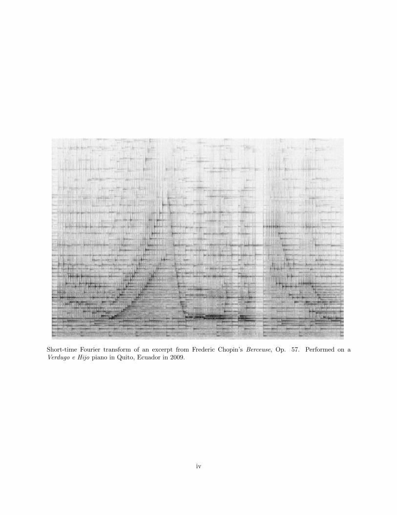
Short-time Fourier transform of an excerpt from Frederic Chopin’s Berceuse, Op. 57. Performed on aVerdugo e Hijo piano in Quito, Ecuador in 2009.

iv

TABLE OF CONTENTS

LIST OF FIGURES . . . . . . . . . . . . . . . . . . . . . . . . . . . . . . . . . . . . . . . . . . . . . . viiLIST OF ALGORITHMS . . . . . . . . . . . . . . . . . . . . . . . . . . . . . . . . . . . . . . . . . . . viii

CHAPTER 1 INTRODUCTION . . . . . . . . . . . . . . . . . . . . . . . . . . . . . . . . . . . . . . 11.1 Geometry of source separation and localization . . . . . . . . . . . . . . . . . . . . . . . . . . 11.2 Multichannel blind source separation . . . . . . . . . . . . . . . . . . . . . . . . . . . . . . . . 2

1.2.1 Beamforming . . . . . . . . . . . . . . . . . . . . . . . . . . . . . . . . . . . . . . . . . 31.2.2 Time-frequency masking . . . . . . . . . . . . . . . . . . . . . . . . . . . . . . . . . . . 31.2.3 Beamforming vs TF masking . . . . . . . . . . . . . . . . . . . . . . . . . . . . . . . . 4

1.3 Direction-of-arrival estimation and tracking . . . . . . . . . . . . . . . . . . . . . . . . . . . . 41.3.1 DOA estimation . . . . . . . . . . . . . . . . . . . . . . . . . . . . . . . . . . . . . . . 41.3.2 Tracking with Bayesian filters . . . . . . . . . . . . . . . . . . . . . . . . . . . . . . . . 51.3.3 Wrapped filtering . . . . . . . . . . . . . . . . . . . . . . . . . . . . . . . . . . . . . . . 51.3.4 Data association ambiguities in multi-source tracking . . . . . . . . . . . . . . . . . . . 6

1.4 Contributions . . . . . . . . . . . . . . . . . . . . . . . . . . . . . . . . . . . . . . . . . . . . . 6

CHAPTER 2 THEORETICAL TOOLS . . . . . . . . . . . . . . . . . . . . . . . . . . . . . . . . . . 82.1 Short-time analysis of non-stationary signals . . . . . . . . . . . . . . . . . . . . . . . . . . . . 8

2.1.1 Short-time Fourier transform . . . . . . . . . . . . . . . . . . . . . . . . . . . . . . . . 82.1.2 Time-frequency masking . . . . . . . . . . . . . . . . . . . . . . . . . . . . . . . . . . . 10

2.2 Directional statistics . . . . . . . . . . . . . . . . . . . . . . . . . . . . . . . . . . . . . . . . . 122.2.1 Directional distributions . . . . . . . . . . . . . . . . . . . . . . . . . . . . . . . . . . . 132.2.2 Sampling from directional distributions . . . . . . . . . . . . . . . . . . . . . . . . . . 152.2.3 Rotations on the unit sphere . . . . . . . . . . . . . . . . . . . . . . . . . . . . . . . . 17

2.3 Fitting mixtures of directional distributions . . . . . . . . . . . . . . . . . . . . . . . . . . . . 182.3.1 Expectation-Maximization . . . . . . . . . . . . . . . . . . . . . . . . . . . . . . . . . . 182.3.2 Fitting a mixture of wrapped Gaussian distributions . . . . . . . . . . . . . . . . . . . 192.3.3 Fitting a mixture of von Mises distributions . . . . . . . . . . . . . . . . . . . . . . . . 202.3.4 Fitting a mixture of von Mises-Fisher distributions . . . . . . . . . . . . . . . . . . . . 22

2.4 Interchannel phase difference features . . . . . . . . . . . . . . . . . . . . . . . . . . . . . . . 222.4.1 Feature extraction . . . . . . . . . . . . . . . . . . . . . . . . . . . . . . . . . . . . . . 232.4.2 Effect of reverberation on IPD features . . . . . . . . . . . . . . . . . . . . . . . . . . 24

2.5 Circular-linear regression . . . . . . . . . . . . . . . . . . . . . . . . . . . . . . . . . . . . . . . 262.5.1 IPDs as circular-linear data . . . . . . . . . . . . . . . . . . . . . . . . . . . . . . . . . 272.5.2 Probabilistic model for circular-linear regression . . . . . . . . . . . . . . . . . . . . . 27

2.6 Direction-of-arrival estimation . . . . . . . . . . . . . . . . . . . . . . . . . . . . . . . . . . . . 272.6.1 Least-squares DOA estimation . . . . . . . . . . . . . . . . . . . . . . . . . . . . . . . 282.6.2 Trigonometric DOA estimation . . . . . . . . . . . . . . . . . . . . . . . . . . . . . . . 30

2.7 Recursive Bayesian filtering . . . . . . . . . . . . . . . . . . . . . . . . . . . . . . . . . . . . . 302.7.1 Bayesian filtering equations . . . . . . . . . . . . . . . . . . . . . . . . . . . . . . . . . 31

v

2.7.2 Kalman filter . . . . . . . . . . . . . . . . . . . . . . . . . . . . . . . . . . . . . . . . . 322.7.3 Particle filter . . . . . . . . . . . . . . . . . . . . . . . . . . . . . . . . . . . . . . . . . 322.7.4 Multi-source tracking with mixture models . . . . . . . . . . . . . . . . . . . . . . . . 36

2.8 RANdom SAmple Consensus (RANSAC) . . . . . . . . . . . . . . . . . . . . . . . . . . . . . 37

CHAPTER 3 BSS AND DOA ESTIMATION FOR MULTIPLE STATIONARY SPEAKERS . . . . 393.1 EM for fitting a mixture of wrapped lines . . . . . . . . . . . . . . . . . . . . . . . . . . . . . 39

3.1.1 Clustering in each frequency band individually . . . . . . . . . . . . . . . . . . . . . . 393.1.2 Clustering across frequencies . . . . . . . . . . . . . . . . . . . . . . . . . . . . . . . . 403.1.3 Drawbacks of EM . . . . . . . . . . . . . . . . . . . . . . . . . . . . . . . . . . . . . . 41

3.2 Circular-linear regression by random sampling . . . . . . . . . . . . . . . . . . . . . . . . . . . 423.2.1 Sequential RANSAC . . . . . . . . . . . . . . . . . . . . . . . . . . . . . . . . . . . . . 423.2.2 Why sequential RANSAC works . . . . . . . . . . . . . . . . . . . . . . . . . . . . . . 43

3.3 Blind source separation and DOA estimation . . . . . . . . . . . . . . . . . . . . . . . . . . . 443.3.1 Blind source separation . . . . . . . . . . . . . . . . . . . . . . . . . . . . . . . . . . . 443.3.2 Direction-of-arrival estimation . . . . . . . . . . . . . . . . . . . . . . . . . . . . . . . 45

3.4 Experiments . . . . . . . . . . . . . . . . . . . . . . . . . . . . . . . . . . . . . . . . . . . . . . 453.4.1 Synthetic multimodal circular-linear data . . . . . . . . . . . . . . . . . . . . . . . . . 453.4.2 Blind source separation . . . . . . . . . . . . . . . . . . . . . . . . . . . . . . . . . . . 463.4.3 Direction-of-arrival estimation . . . . . . . . . . . . . . . . . . . . . . . . . . . . . . . 473.4.4 Comparison with Bartlett beamformer and MUSIC . . . . . . . . . . . . . . . . . . . . 48

CHAPTER 4 DIRECTION-OF-ARRIVAL TRACKING WITH IPD FEATURES . . . . . . . . . . . 524.1 Bayesian tracking on the unit circle . . . . . . . . . . . . . . . . . . . . . . . . . . . . . . . . . 52

4.1.1 State space models for wrapped filtering . . . . . . . . . . . . . . . . . . . . . . . . . . 534.1.2 Wrapped Kalman filter (WKF) . . . . . . . . . . . . . . . . . . . . . . . . . . . . . . . 544.1.3 WKF as an approximation of a switching Kalman filter . . . . . . . . . . . . . . . . . 564.1.4 Discussion of the WKF . . . . . . . . . . . . . . . . . . . . . . . . . . . . . . . . . . . 574.1.5 Factorial wrapped Kalman filter (FWKF) . . . . . . . . . . . . . . . . . . . . . . . . . 584.1.6 Derivation of FWKF . . . . . . . . . . . . . . . . . . . . . . . . . . . . . . . . . . . . . 594.1.7 FWKF as an approximation of a switching Kalman filter . . . . . . . . . . . . . . . . 604.1.8 Discussion of FWKF . . . . . . . . . . . . . . . . . . . . . . . . . . . . . . . . . . . . . 61

4.2 Bayesian tracking on the unit sphere . . . . . . . . . . . . . . . . . . . . . . . . . . . . . . . . 624.2.1 Von Mises-Fisher particle filter (vMFPF) . . . . . . . . . . . . . . . . . . . . . . . . . 634.2.2 Factorial von Mises-Fisher particle filter (FvMFPF) . . . . . . . . . . . . . . . . . . . 644.2.3 Discussion of FvMFPF . . . . . . . . . . . . . . . . . . . . . . . . . . . . . . . . . . . 65

4.3 Bayesian tracking with raw IPD features . . . . . . . . . . . . . . . . . . . . . . . . . . . . . . 664.3.1 State space model . . . . . . . . . . . . . . . . . . . . . . . . . . . . . . . . . . . . . . 674.3.2 Tracking on the unit circle with a von Mises particle filter (vMPF) . . . . . . . . . . . 67

4.4 Experiments . . . . . . . . . . . . . . . . . . . . . . . . . . . . . . . . . . . . . . . . . . . . . . 684.4.1 Single source tracking on the unit circle . . . . . . . . . . . . . . . . . . . . . . . . . . 694.4.2 Multi-source tracking on the unit circle . . . . . . . . . . . . . . . . . . . . . . . . . . 704.4.3 Multiple speaker tracking on the unit sphere . . . . . . . . . . . . . . . . . . . . . . . 71

CHAPTER 5 CONCLUDING THOUGHTS . . . . . . . . . . . . . . . . . . . . . . . . . . . . . . . . 73

APPENDIX A VON MISES/VON MISES-FISHER AS A CONDITIONED GAUSSIAN . . . . . . . 75

APPENDIX B DERIVATION OF TRIGONOMETRIC DOA ESTIMATORS . . . . . . . . . . . . . 77

REFERENCES . . . . . . . . . . . . . . . . . . . . . . . . . . . . . . . . . . . . . . . . . . . . . . . . . 82

vi

LIST OF FIGURES

1.1 Geometry of source separation and localization . . . . . . . . . . . . . . . . . . . . . . . . . . 2

2.1 Time-domain speech waveform and spectrogram . . . . . . . . . . . . . . . . . . . . . . . . . 92.2 Clean and mixed speech spectrograms . . . . . . . . . . . . . . . . . . . . . . . . . . . . . . . 112.3 Ideal binary masks . . . . . . . . . . . . . . . . . . . . . . . . . . . . . . . . . . . . . . . . . . 122.4 Spectrograms of separated speech . . . . . . . . . . . . . . . . . . . . . . . . . . . . . . . . . . 122.5 Two visualizations of the wrapped Gaussian distribution . . . . . . . . . . . . . . . . . . . . . 142.6 Contours of the von Mises-Fisher distribution on the unit sphere . . . . . . . . . . . . . . . . 152.7 Relationship between κ and σ2 for importance sampling from the vM . . . . . . . . . . . . . 172.8 Effect of reverb on IPD features . . . . . . . . . . . . . . . . . . . . . . . . . . . . . . . . . . . 252.9 IPD plot for synthetic mixture of three sources . . . . . . . . . . . . . . . . . . . . . . . . . . 262.10 Circular-linear data and IPD model log likelihood . . . . . . . . . . . . . . . . . . . . . . . . . 282.11 Geometry of least-squares DOA estimation . . . . . . . . . . . . . . . . . . . . . . . . . . . . 292.12 Graphical model of dynamic Bayesian network. . . . . . . . . . . . . . . . . . . . . . . . . . . 302.13 Sequential importance resampling for particle filtering . . . . . . . . . . . . . . . . . . . . . . 352.14 Line-fitting with RANSAC in uniform noise and 50% outliers . . . . . . . . . . . . . . . . . . 38

3.1 Graphical model for wrapped-line fitting . . . . . . . . . . . . . . . . . . . . . . . . . . . . . . 403.2 Example of sequential RANSAC for wrapped line-fitting . . . . . . . . . . . . . . . . . . . . . 433.3 IPD plot of highly reverberant, real-world, stereo recording of two male speakers . . . . . . . 433.4 Models fit by sequential RANSAC . . . . . . . . . . . . . . . . . . . . . . . . . . . . . . . . . 463.5 BSS Eval results for source separation using sequential RANSAC . . . . . . . . . . . . . . . . 473.6 Likelihood surface for synthetic 4-speaker localization . . . . . . . . . . . . . . . . . . . . . . 483.7 Likelihood surfaces of sequential RANSAC in each iteration . . . . . . . . . . . . . . . . . . . 503.8 SRP-PHAT response power, MUSIC spectrum, and IPD likelihood . . . . . . . . . . . . . . . 51

4.1 Sample path, observation sequence, and WKF estimate for wrapped dynamical system . . . . 544.2 Two interpretations of the correct step in the WKF . . . . . . . . . . . . . . . . . . . . . . . 554.3 Graphical model of switching dynamic Bayesian network. . . . . . . . . . . . . . . . . . . . . 574.4 Graphical model of factorial wrapped dynamical system . . . . . . . . . . . . . . . . . . . . . 584.5 Sample paths, observations sequences, and FWKF estimates for factorial WDS . . . . . . . . 614.6 MSE of EKF, UKF, and WKF for tracking on the unit circle . . . . . . . . . . . . . . . . . . 694.7 Likelihoods of factorial EKF and FWKF for tracking on the unit circle . . . . . . . . . . . . . 704.8 DOA tracking on the unit circle with the FWKF for 2 speakers . . . . . . . . . . . . . . . . . 714.9 DOA tracking on the unit sphere with the FvMFPF for 2 speakers . . . . . . . . . . . . . . . 72

A.1 2D Gaussian on the unit circle . . . . . . . . . . . . . . . . . . . . . . . . . . . . . . . . . . . 76

B.1 Geometry of localization on a semicircle and circle . . . . . . . . . . . . . . . . . . . . . . . . 78B.2 Geometry of localization on a hemisphere . . . . . . . . . . . . . . . . . . . . . . . . . . . . . 79B.3 Geometry of localization on the unit sphere . . . . . . . . . . . . . . . . . . . . . . . . . . . . 80

vii

LIST OF ALGORITHMS

1 EM for fitting a mixture of wrapped Gaussian distributions . . . . . . . . . . . . . . . . . . . 20

2 EM for fitting a mixture of von Mises distributions . . . . . . . . . . . . . . . . . . . . . . . . 21

3 EM for fitting a mixture of von-Mises Fisher distributions . . . . . . . . . . . . . . . . . . . . 23

4 Kalman filter . . . . . . . . . . . . . . . . . . . . . . . . . . . . . . . . . . . . . . . . . . . . . 32

5 Particle filter - sequential importance resampling . . . . . . . . . . . . . . . . . . . . . . . . . 34

6 RANSAC . . . . . . . . . . . . . . . . . . . . . . . . . . . . . . . . . . . . . . . . . . . . . . . 38

7 EM for fitting a mixture of multi-band wrapped Gaussian distributions . . . . . . . . . . . . . . . 41

8 Sequential RANSAC for fitting multiple wrapped lines . . . . . . . . . . . . . . . . . . . . . . 42

9 Wrapped Kalman filter . . . . . . . . . . . . . . . . . . . . . . . . . . . . . . . . . . . . . . . . 56

10 Factorial wrapped Kalman filter . . . . . . . . . . . . . . . . . . . . . . . . . . . . . . . . . . 59

11 Von Mises-Fisher particle filter . . . . . . . . . . . . . . . . . . . . . . . . . . . . . . . . . . . 63

12 Factorial von Mises-Fisher particle filter . . . . . . . . . . . . . . . . . . . . . . . . . . . . . . 65

13 Von Mises particle filter with raw IPD features . . . . . . . . . . . . . . . . . . . . . . . . . . 68

viii

CHAPTER 1

INTRODUCTION

This chapter reviews the blind source separation (BSS) and localization problems and a number of techniques

that have been applied to solve them. Particular attention is given to multichannel methods that use an

array of microphones to incorporate spatial information into the separation. We first describe the physical

geometry involved. Then, we briefly review beamforming (the classical approach to array processing) and

time-frequency (TF) masking. The latter approach is a BSS method designed specifically for the class of

signals that tend to satisfy a disjointness property. Speech is conveniently a member of this class. Following

this is a discussion of methods for direction-of-arrival (DOA) estimation. We also review tracking algorithms

from the Bayesian filtering literature as we often cannot assume that the sources are physically stationary.

Then, methods for tracking multiple sources on the unit circle and sphere with mixtures of directional

distributions are introduced. Finally, we summarize the contributions of this thesis.

1.1 Geometry of source separation and localization

To understand the multichannel source separation and localization problem, we start by looking at the

physical geometry involved. We have an array with C microphones placed in a room with K sound sources.

This is depicted for C = 3, K = 2, and a rectangular room in Figure 1.1. In anechoic conditions, each

speaker is recorded by each microphone only once with an attenuation and delay that depends solely on the

distance between them. The direct-path delay from the jth source to the ith microphone is denoted as dij .

When the room is reverberant, multiple copies of each source signal will be recorded at each microphone,

where each copy is an attenuated and delayed version of the original source signal. We will not explicitly

model reverberation in this thesis. Instead, we will design algorithms that are robust to its effects.

To solve the source separation problem, we need to partition one of the recordings into K parts corre-

sponding to each of the speakers. We can use the array to estimate the directions of the sources. Methods

for isolating energy from a particular direction can then be applied to do the separation. The Degenerate

Unmixing Estimation Technique [1] is a famous example of this. Intuitively, we would like to design al-

gorithms that perform better as more microphones become available and that are robust to the effects of

unknown interference and complicated reverberation.

1

2  

1

3

d11

d12

d21

d22

d32

d31

1

2  

Figure 1.1: Geometry of the multichannel source separation and localization problem for K = 2 sourcesand C = 3 microphones (a.k.a. Wolfie and Ludwig in an argument). dij denotes the time taken for soundto propagate from source j to microphone i. Examples of first- and second-order reflections are shown asdashed lines. (The microphone separation is exaggerated for ease of interpretation.)

1.2 Multichannel blind source separation

Human beings have the remarkable ability to focus on a single speaker in a crowded, noisy environment. This

is called the “cocktail party effect” and is at the center of literature on Auditory Scene Analysis (ASA) [2].

Studies in the neuroscience community on audition have revealed that the human brain does indeed perform

some kind of source separation [3]. Reconstructed signals from brain scans show the salient information

corresponding only to the speaker of interest, as if the other speaker(s) were not present in the experiment.

This is a fascinating result that further motivates the design of automated BSS algorithms.

The literature on multichannel BSS algorithms is vast [4], [5], [6]. Independent components analysis (ICA)

is one famous approach that attempts to invert a mixing matrix relating the source signals to the recorded

mixtures. This matrix contains all the relevant attenuation and delay information about how the signals

propagate toward the microphones. More recently, matrix decomposition techniques such as Nonnegative

Matrix Factorization [7], [8] have been applied directly to the speech spectrogram. NMF has a desirable

parts-based representation of the input that aligns very well with the additive nature of sounds.

In this thesis, we will focus on the time-frequency masking approach outlined in [1], which takes advantage

of disjointness of speech signals in a time-frequency representation. However, a discussion of multichannel

audio would not be complete without a review of the classical approach to array processing: beamforming.

2

1.2.1 Beamforming

Beamforming methods [9], [10] [11], [12], [13] approach source separation/enhancement from a classical

array processing perspective. This involves designing a spatial filter that can be steered without moving

any physical parts of the array. In general, the filter is designed to allow signals impinging on the array

from particular directions to pass undistorted while blocking interfering signals incident at other angles. The

filter’s lobes in the desired directions are called “beams” and its zeros in the undesired directions are called

“nulls,” hence the terminology “beam-steering” and “null-steering.”

The simplest case is that of a single directional source in ambient white noise. The optimal spatial filter,

in terms of signal-to-noise ratio (SNR), is the delay-and-sum (D&S) beamformer. It delays the microphone

recordings such that the source signals are aligned and then sums over the channels. This is straightforward

once the DOA is known because there is a simple mapping from DOA to inter-channel delays. When the

ambient noise is more structured (i.e. the noise in the channels is correlated), then we can do better with

the minimum-variance distortionless response (MVDR) beamformer. For a narrowband signal, the MVDR

keeps track of a channel covariance matrix and uses it to pre-whiten the inputs and further suppress noise.

However, if the noise is white, the MVDR reduces to the D&S.

If multiple desired sources and directional interferers are active simultaneously, we desire a spatial filter

that enforces multiple distortionless constraints and blocks the interferers. At most C such constraints

can be applied at once. A flexible algorithm to achieve this is the linearly-constrained minimum-variance

(LCMV) beamformer, which requires the solution to a constrained optimization problem. We can implement

it efficiently by using a generalized sidelobe canceler (GSC) structure [14]. This involves separating the

constraints into two orthogonal sets corresponding to beams and nulls and processing the input along two

separate branches. The outputs are then combined to produce a final result.

1.2.2 Time-frequency masking

The Degenerate Unmixing Estimation Technique (DUET) [1] and its extension to more than 2 micro-

phones [15] are based on time-frequency (TF) masking. This involves clustering of inter-channel phase

and level differences (IPD, ILD) to construct a binary TF mask and is known to produce extremely clean

separation of speech in non-reverberant environments. The two assumptions in DUET are that the source

signals are approximately disjoint in a time-frequency representation and that at most one sample of delay

is observed between the channels. Speech signals are remarkably disjoint in the short-time Fourier transform

(STFT) even in the presence of strong reverberation [16]. Thus, the first assumption often holds. However,

for high sampling rates or arrays with more than a few centimeters of separation between the microphones,

spatial aliasing violates the second assumption. Spatial aliasing occurs when the incoming signal contains

energy with a wavelength that is less than half the inter-mic spacing. Solutions include oversampling [17]

and explicit modeling of phase as a wrapped quantity [18], [19], [20]. We will adopt the latter approach in

this thesis.

3

1.2.3 Beamforming vs TF masking

A desirable property of beamforming methods is the distortionless constraint. This is important, for example,

in speech enhancement algorithms where even a moderate amount of artifacts in a speaker’s voice can cause

discomfort to the listener. However, the drawback is that they are not designed with source separation

in mind. Time-frequency (TF) masking, in contrast, was designed specifically for separating TF-disjoint

signals such as speech. The ideal mask achieves near-perfect separation with only two microphones, even

in the presence of strong reverberation. Another concern is that most beamforming methods assume a

large number of widely-spaced channels (e.g. 10 or more) are available. This is an infeasible constraint

for handheld devices. Furthermore, the criteria that beamformers typically optimize involve SNR, which is

known to correlate poorly with separation quality [21]. Other metrics such as signal-to-interference ratio

(SIR) are more informative. SIR, along with signal-to-distortion ratio (SDR) and signal-to-artifact ratio

(SAR), have been defined in [21] for evaluating BSS algorithms.

1.3 Direction-of-arrival estimation and tracking

Array-based source localization has been an important area of research for many decades [22], [23]. The goal

is to determine the position(s) of the source(s) relative to the array using only the recorded signals. For

compact arrays with less than 10 cm of spacing between any pair of microphones, the far-field model is often

used as a simplifying assumption. This says that the shape of the signal wavefront emitted by the source is

well-approximated as planar by the time it reaches the array. For small arrays, we are better off tracking

the direction-of-arrival (DOA) of a source rather than its physical position in the room as it is too difficult

to estimate its distance to the array. We also need a method for following it as it moves about. Multi-target

tracking algorithms generalize this idea to the case that we care about. In this thesis, algorithms for tracking

multiple speakers on the unit circle and sphere are proposed that approach the problem from a Bayesian

perspective.

1.3.1 DOA estimation

Consider the simple case of one source and a two-microphone array. The easiest approach to estimating the

DOA is to compute the cross-correlation between the channels [24]. In the presence of moderate ambient

noise, a peak will appear at the inter-channel delay corresponding to the source’s position. This can be

extended by applying a pre-whitening filter such as the PHAse Transform (PHAT) before the correlation.

This is called the generalized cross correlation (GCC) method. A multichannel GCC (MCCC) method was

developed for when more than 2 channels are available [25]. Alternatively, one can quickly compute the GCC

on a grid in DOA space [26], [27]. A similar approach computes the steered response power (SRP) function,

which is simply the response of your favorite beamformer as its beam is swept over DOA space [13].

Another well-known approach is the MUltiple SIgnal Classification (MUSIC) algorithm [28], which requires

that more channels are available than there are sources (i.e. C > K). The MUSIC algorithm is based on the

idea that the frequency-domain channel covariance matrix Σ contains orthogonal signal and noise subspaces.

The first K eigenvectors of Σ span the space of steering vectors, ς, corresponding to the source DOAs θi

4

and the remaining C −K eigenvectors span the noise (null) space. The norm ‖Σs ς(θ)‖2 will be large if θ

corresponds to a source direction and small otherwise, where Σs is the matrix whose columns span the signal

subspace. We can compute this value over all directions θ to calculate a “pseudospectrum” with multiple

peaks, one for each source. The pseudospectrum is usually calculated using the noise subspace matrix:

‖Σn ς(θ)‖−12 .

Many variations on the basic MUSIC algorithm exist including root-Music [29], which finds the roots of

a polynomial, and Estimation of Signal Parameters via Rotational Invariance Techniques (ESPRIT) [30],

which takes advantage of special array structures. The DUET and ESPRIT methods were combined to form

DESPRIT [31].

1.3.2 Tracking with Bayesian filters

Multichannel BSS algorithms are often made spatially adaptive to separate moving sources by tracking

their directions-of-arrival (DOA) over time. This is typically done by applying the GCC or MUSIC methods

adaptively on a short-term basis [32]. However, the estimates may be noisy, especially in reverberant environ-

ments, so we would ideally like to smooth them out. This motivates tracking with the Kalman filter [33], [34]

and related methods.

The Bayesian filtering framework allows for sophisticated, statistically-grounded approaches to tracking.

The dynamical systems involved are often non-linear, so the extended Kalman filter (EKF) [35] and unscented

Kalman filter (UKF) [36] are used to linearize the dynamics. The EKF uses a first-order Taylor series

expansion of the non-linearity. This may be inadequate as the approximation fails to capture higher-order

effects. The UKF remedies this by choosing a number of deterministically-chosen “sigma points” that are fed

through the system dynamics. This approach uses the unscented transform [37] to keep track of higher-order

statistics.

For highly non-linear, non-Gaussian systems, the particle filter (PF) is a flexible alternative [38], [39], [40], [41].

More sophisticated strategies use the EKF or UKF as a sub-component in the PF to reduce the variance

of the state estimate [42], [43]. This is especially effective in noisy, reverberant environments [44]. The

Gaussian sum filter (GSF) [45] and its extensions [46], [47], [48], in particular, are important as they enable

the tracking of non-Gaussian and possibly multimodal state distributions. An extension of GSF techniques

leads to particle filters that are designed for the complicated task of tracking multiple sources simultane-

ously [43], [49], [50], [51].

1.3.3 Wrapped filtering

In this thesis, we are interested in tracking on the unit circle and sphere. This shows up in many applications

including phase-locked loops [52], phase unwrapping [53], source localization [9], and more. Work on 2D phase

unwrapping motivates use of the Kalman filter framework [54], [55] for circular data. However, deterministic

methods have also been explored in [56], [57].

Our primary goal is to design Bayesian filters that operate directly on the unit circle and sphere. This

is in contrast to many approximate methods that model these spaces indirectly by, for example, filtering in

the embedding spaces: R2 and R3. We will use the wrapped Gaussian (WG) distribution [58] to derive a

5

wrapped Kalman filter (WKF) for tracking a wrapped dynamical system (WDS). We will show that modeling

the state of the WDS explicitly with a directional distribution reduces the tracking variance significantly

over 2D Gaussian methods. The WG has also been used to learn source trajectories with a wrapped-phase

hidden Markov model [59]. A WG state model has the advantage of being closely related to the conventional

Gaussian distribution for which optimal inference procedures exist. We will use a mixture of WGs [60] to

extend the WKF to the case of multiple sources, yielding the factorial wrapped Kalman filter (FWKF).

The von Mises-Fisher (vMF) distribution [58] has been used to model the state distribution of a dynamical

system on the unit sphere [61]. We adopt this strategy and generalize it by modeling the state distribution

with a mixture of vMFs to yield the factorial von Mises-Fisher particle filter (FvMFPF). In speaker tracking

problems with a compact array in 3 dimensions, it is infeasible to estimate range values (i.e. distance to the

target). Thus, the localization problem is more appropriately posed as that of estimating directions-of-arrival

(DOA) only. The FvMFPF is a natural solution since it models the source positions explicitly on the sphere.

1.3.4 Data association ambiguities in multi-source tracking

The main complication with extending filters to handle multiple sources is the data association problem. We

will assume that each source evolves independently of the others and generates its own observation sequence.

However, one observes the unordered set of measurements. Two famous methods for resolving this ambiguity

are Probabilistic Data Association (PDA) [62] and Multiple Hypothesis Tracking (MHT) [63]. The PDA

approach combines measurements in a probabilistic fashion so that all the data gets its (proportional)

chance to affect the state estimate. On the other hand, MHT keeps track of several hypotheses about

how measurements are associated to target tracks. These are propagated into the future in the hopes that

any ambiguities will quickly be resolved with additional data. This problem has also been tackled via

acceptance region methods [64], hidden Markov modeling, [65], Gaussian mixture modeling of time-delay-

of-arrival data [66], recursive EM-based approaches [67], [68], and a particle filter with TF masking-based

data association [69]. Particle filtering strategies for acoustic DOA tracking have also been explored in [70]

and [71]. In this thesis, we will use soft assignments of measurements/particles to clusters in the FWKF and

FvMFPF to effectively “integrate out” the ambiguities. This is most aligned with the PDA framework and

fits naturally in the probabilistic framework of Bayesian filtering with mixtures.

1.4 Contributions

In previous work [20], the von Mises distribution [58] was used to model wrapped inter-channel phase

difference (IPD) features as circular-linear data [72]. The features are modified from those presented in [1]

to explicitly incorporate spatial aliasing into a statistical model. The BSS problem was reduced to one of

multimodal circular-linear regression, which can be interpreted as fitting several helices to data that lies on

a cylinder. The RANdom SAmple Consensus (RANSAC) algorithm [73] was applied to quickly and robustly

perform the fitting.1 The resulting wrapped lines provide a clustering of the features and thus a method for

constructing time-frequency masks.

1A similar approach was taken in [74]. RANSAC was also used for source localization in [75].

6

In this thesis, we consider the use case of speaker separation with a microphone array when the sources

are stationary and when they are moving [76], [77], [78]. The filters presented here require a method by

which DOA votes can be extracted from the recorded speech to be used as measurements. We will apply the

IPD clustering algorithm from [20] to extract short-time DOA estimates. Alternatively, a von Mises particle

filter (vMPF) is proposed that uses the IPD features directly as observations. We present the WKF, FWKF,

vMFPF, FvMFPF, and vMPF not as complete DOA tracking systems, which can be highly elaborate, but

as potential components in such an engine.

The contributions of this thesis are:

• a probabilistic formulation for the wrapped IPD clustering problem

• a detailed account of the RANSAC-based source separation algorithm presented in [20]

• the wrapped Kalman filter (WKF) for tracking a moving source on the unit circle

• the factorial wrapped Kalman filter (FWKF), an extension of the WKF for multi-source tracking on

the unit circle

• the factorial von Mises-Fisher particle filter (FvMFPF) for multi-source tracking on the unit sphere

• the von Mises particle filter (vMPF) for tracking on the unit circle with raw IPD features

• a discussion of the measurement/particle assignment ambiguities involved in multi-source tracking and

how the proposed filters resolve them in a Bayesian setting

• experiments demonstrating the utility of the proposed methods for tracking and separating speakers

with a microphone array

7

CHAPTER 2

THEORETICAL TOOLS

This chapter serves as a collage of theoretical machinery that will be used in the rest of the thesis. The

short-time Fourier transform (STFT) is introduced as a means to convert time-domain signals received at the

microphones into a more useful time-frequency representation. Useful theory from the directional statistics

literature and EM algorithms to fit mixtures of directional distributions are reviewed. Then, inter-channel

differences (IPD) are extracted from the channel STFTs. It is shown that these features compose a circular-

linear dataset and that wrapped lines in IPD space correspond to speakers. The blind source separation

problem is thus reduced to one of multimodal circular-linear regression. The direction-of-arrival (DOA)

of a speaker is related to the slope of an IPD line, showing that solving the wrapped line-fitting problem

automatically provides an estimate of the source positions. Following this is a review of the Bayesian filtering

framework including particle filtering and tracking with mixture models in the presence of data association

ambiguities. Finally, the RANdom SAmple Consensus (RANSAC) algorithm is presented as a fast, heuristic

approach to line-fitting that is highly robust to outliers.

2.1 Short-time analysis of non-stationary signals

A discrete-time sound signal

x = [x[0], x[1], . . . , x[n], . . . , x[N − 2], x[N − 1]] (2.1)

is a sampled version of an acoustic waveform recorded by a microphone. In this thesis, we will work

with the short-time Fourier transform (STFT) [79] of x as this provides a more useful and interpretable

representation of its contents. A discrete-time speech signal and the magnitude portion of its STFT (also

called a spectrogram) are shown in Figure 2.1. The signal’s statistics across frequency and time are far more

apparent in the latter figure. We can see the distinctive speech harmonics during vowels, for example, and

high-frequency broadband noise bursts during “s” and “t” sounds.

2.1.1 Short-time Fourier transform

The STFT is a sequence of overlapping discrete Fourier transforms (DFT) [79]. The DFT is defined as the

mapping F : CN → CN such that:

8

Time (frames)

Freq

uenc

y (b

ands

)

20 40 60 80 100 120

50

100

150

200

250

300

350

400

450

500

Figure 2.1: (Top) Time domain waveform of a female TSP speaker saying “the lease ran out in sixteenweeks.” (Bottom) Magnitude of the corresponding short-time Fourier transform. Brightness indicates howmuch energy is contained in each time-frequency bin.

X[f ] = F (x) =

N−1∑

n=0

x[n]e−j2πfN n , (2.2)

and the inverse DFT is similarly defined as the mapping F−1 : CN → CN such that:

x[n] = F−1 (X) =1

N

N−1∑

f=0

X[f ]ej2πfN n . (2.3)

Since speech is non-stationary (it changes with time), we would like to define a transformation to the

Fourier domain that depends on time. The STFT is exactly what we need and is defined as the mapping

STFT (x) : CM → CN×T , where N = 2D is the length of each DFT and T is the number of frames required

to capture the non-zero content in the signal:

9

Xt[f ] = F (w � xt) =

N−1∑

n=0

w[n]xt[n]e−j2πfN n , xt[n] = x[n+ th] . (2.4)

The symbol � indicates element-wise multiplication and w ∈ RN is an analysis window function used to

select and weight a portion of the time-domain signal for each DFT. The signal is shifted so that the window

captures the samples required for the tth DFT. The shift is parameterized by a hop size h that is typically

chosen to be one quarter of the window length: h = N/4. Audio signals are real-valued, so the DFT will

satisfy a symmetry property: the first D coefficients will be the reversed complex conjugate of the last D

coefficients. Thus, we can discard the second half during processing as it provides no additional information.

The analysis window is useful to prevent artifacts in time-domain reconstructions when alterations are

made to the STFT. Such alterations are common in source separation algorithms. We choose the Hanning

window:

w[n] =

0.5− 0.5 cos(

2πnN−1

), 0 ≤ n ≤ N − 1

0 , else(2.5)

because it conveniently tapers to zero at the boundaries and is known to produce high-quality reconstructions

in BSS applications compared to most other choices.

To reconstruct a time-domain signal from a (possibly modified) STFT X, we apply the inverse STFT

using the analysis window as a synthesis window:

x =

T−1∑

t=0

[w �F−1

(Xt

)]∗ δ[n− th] , (2.6)

where ∗ denotes convolution and δ[n − k] is the Kronecker delta shifted by k samples. The convolution

operation shifts the windowed inverse DFTs into place. A condition for perfect reconstruction from an

unaltered STFT is that the sum of squared windows:

ws[n] =T−1∑

t=0

w[n− th]2 , (2.7)

remain constant over the domain where the signal is non-zero [80]. If it does not, we should divide the

reconstruction element-wise by this sum. However, if we choose the hop size to be a quarter of the window

length and we use a Hanning window, the optimality condition is satisfied and no division is necessary.

2.1.2 Time-frequency masking

A special property of speech signals is that they tend not to overlap in the STFT. This is known as W-disjoint

orthogonality [16], or simply disjointness, and is very useful for source separation using time-frequency (TF)

masks [1]. Consider the case of two speaker signals s(1) and s(2) with STFTs S(1) and S(2) that are active

simultaneously (they are talking over each other). Spectrograms of the clean speech signals from the TSP

10

Time (frames)

Fre

qu

en

cy (

ba

nd

s)

20 40 60 80 100 120

50

100

150

200

250

300

350

400

450

500

Time (frames)

Fre

qu

en

cy (

ba

nd

s)

20 40 60 80 100 120

50

100

150

200

250

300

350

400

450

500

(a)

Time (frames)

Fre

quen

cy (

band

s)

20 40 60 80 100 120

50

100

150

200

250

300

350

400

450

500

(b)

Figure 2.2: Clean and mixed speech spectrograms. (a) Spectrograms of one female (left) and one male (right)TSP speaker. The sentences are “the lease ran out in sixteen weeks” and “the slab was hewn from heavyblocks of slate.” (b) Spectrogram of two TSP speakers after mixing. Disjointness of speech in the STFTdomain allows us to approximate the mixture spectrogram as the sum of the clean speech spectrograms.

database [81] and their mixture are shown in Figure 2.2(a) and Figure 2.2(b). The signals are considered to

be disjoint if

∀ t, f S(1)t,f · S

(2)t,f = 0 . (2.8)

The ideal binary mask (IBM) needed to reconstruct approximations of the individual speakers is a matrix

M of ones and zeros such that:

Mt,f =

1 , |S(1)t,f |2 > |S

(2)t,f |2

0 , otherwise. (2.9)

Applying this mask element-wise to the mixture, X = STFT(s(1) + s(2)

), will isolate the energy from the

first speaker. Similarly, applying the inverse mask, 1−M, will isolate the energy from the second speaker.

IBMs for the example signals are shown in Figure 2.3. The inverse STFT can then be applied to the masked

STFTs to reconstruct separated time-domain signals. Spectrograms of the separated signals are shown in

11

Time (frames)

Fre

qu

en

cy (

ba

nd

s)

20 40 60 80 100 120

50

100

150

200

250

300

350

400

450

500

Time (frames)

Fre

qu

en

cy (

ba

nd

s)

20 40 60 80 100 120

50

100

150

200

250

300

350

400

450

500

Figure 2.3: Ideal binary masks (IBM) for separating the two speakers from the mixture. The IBM assignstime-frequency bins according to which of the two speakers has the most energy.

Time (frames)

Fre

qu

en

cy (

ba

nd

s)

20 40 60 80 100 120

50

100

150

200

250

300

350

400

450

500

Time (frames)

Fre

qu

en

cy (

ba

nd

s)

20 40 60 80 100 120

50

100

150

200

250

300

350

400

450

500

Figure 2.4: Spectrograms of separated speech after applying time-frequency masks. Comparing this to theoriginal spectrograms shows that masking works extremely well for speech.

Figure 2.4. The IBM is considered optimal in the sense that it maximizes the signal-to-noise ratio (SNR)

of either reconstruction [82]. Binary TF masking has been shown to give very good separation results in

anechoic conditions precisely because of the disjointness of speech signals in the STFT [1]. One drawback

is that a poorly-estimated mask can introduce distracting musical noise. In practice, further processing is

needed to clean up the separation.

2.2 Directional statistics

In this section, we review material from the directional statistics literature [58], [83], [84] that will be useful

for modeling phase in the STFT and the direction-of-arrival (DOA) of a sound source. This includes the

wrapped Gaussian (WG) and von Mises (vM) distributions on the unit circle and the von Mises-Fisher

(vMF) distribution on the unit sphere as well as algorithms for sampling from them. Rotations on the unit

sphere are also discussed as this will be useful for speaker tracking.

12

2.2.1 Directional distributions

We will find use for statistical models of circular quantities. Classic examples are time of day, wind direction,

and sinusoidal phase. Such quantities cannot be modeled with a distribution on the real line, R1, because

they actually lie on a sub-interval of R1, i.e. [0, 12] or [−π, π]. The latter set defines the wrapped interval

S1 = {θ : θ ∈ [−π, π]} . (2.10)

Alternatively, we can represent each scalar angle with a unit vector in R2:

S1 = {x : ‖x‖2 = 1 , x ∈ R2} . (2.11)

Both define a valid wrapped sample space since the endpoints represent the same index, but we will find the

former representation more useful.

An intuitive way to understand the nature of S1 is to consider an appropriate measure of centrality. On

the real line, the arithmetic mean of a dataset X = {xi}, i = 1, . . . , N , is calculated as

µ =1

N

N∑

i=1

xi . (2.12)

This is the maximum-likelihood estimator (MLE) of the mean for data that is assumed to have been sampled

from a Gaussian distribution. However, consider a dataset of angle measurements θ = {θi}, i = 1, . . . , N

that lie on the interval [−π, π]. If they are concentrated near the boundaries −π and π, the arithmetic mean

will return a value near 0, which is incorrect. Instead, we should calculate a circular measure of centrality:

µ = ∠N∑

i=1

ejθi = ∠

(N∑

i=1

cos(θi) + j sin(θi)

)= tan−1

N∑i=1

sin(θi)

N∑i=1

cos(θi)

. (2.13)

This is an unbiased estimator for the mean of a wrapped Gaussian (WG) distribution and the MLE for the

mean of a von Mises (vM) distribution.

Wrapped Gaussian distribution

The probability density function (pdf) of the WG is given as:

P(θ ; µ, σ2

)=

∞∑

l=−∞

1√2πσ2

e−(θ−µ+2πl)2

2σ2 , −π ≤ θ ≤ π , (2.14)

and is the result of transforming a Gaussian random variable x via the mapping ψ : R1 → S1:

θ = ψ(x) = mod(x+ π, 2π)− π . (2.15)

We can visualize the WG on the unit circle in R2 (left panel of Figure 2.5) or directly in S1 (right panel

13

−π −2 π / 3 −π / 3 0 π / 3 2 π / 3 π

0.1

0.2

0.3

0.4

0.5

0.6

0.7

0.8

θ

σ2 = 0.2

σ2 = 1

σ2 = 3

Figure 2.5: (Left) Wrapped Gaussian pdf (µ = π3 ) on the unit circle in R2 shown with 2D Gaussian contours

(σ2 = 0.8). (Right) WG pdf in [−π, π] (µ = π3 and varying σ2). The θ axis is the unit circle, unfolded.

of Figure 2.5). Its close relationship with the conventional univariate Gaussian distribution will make it

possible to derive approximate closed-form expressions for several algorithms in this thesis.

von Mises distribution

We will also find use for the von Mises (vM) distribution. The pdf of the vM is given as

P (θ ; µ, κ) =1

2πI0(κ)eκ cos(θ−µ) , −π ≤ θ ≤ π , (2.16)

and is the result of conditioning a 2D Gaussian, N(µ, σ2I

), ‖µ‖2 = 1, on the unit circle and converting from

Cartesian to polar coordinates (see Appendix A). The conditioning results in that κ = 1/σ2. The vM may

be more convenient than the WG when we only care to evaluate the pdf rather than derive an algorithm.

The vM becomes a Dirac delta at µ for κ→∞ and the uniform distribution on S1 for κ→ 0. It looks very

similar to the WG.

von Mises-Fisher distribution

We can define a sample space on the unit sphere:

S2 = {x : ‖x‖2 = 1 , x ∈ R3} . (2.17)

This representation turns out to be most convenient, although an equivalent parameterization in terms of

spherical coordinates (azimuth θ and zenith φ) is:

S2 = {[θ, φ] : θ ∈ [−π, π] , φ ∈ [0, π]} . (2.18)

The latter definition is less useful in general because it defines a 2D rectangle that results from applying a

14

Figure 2.6: Contours of the von Mises-Fisher distribution on the unit sphere for three values of the concen-tration parameter κ.

highly non-linear mapping to the former (degenerate) 3D set. This complication arises from the fact that it

is impossible to gracefully wrap a rectangle around a sphere.

The classic distribution on the unit sphere is a generalization of the von Mises called the von Mises-Fisher

(vMF). It is parameterized by a mean direction µ , ‖µ‖2 = 1, and concentration κ:

P (x ; µ, κ) =κ

2π (eκ − e−κ)eκxTµ , x ∈ S2 . (2.19)

The contours of various vMFs are depicted in Figure 2.6. The vMF can be derived by conditioning a 3D

Gaussian, N(µ, σ2I

), ‖µ‖2 = 1, on the unit sphere (see Appendix A). It becomes a Dirac delta at µ for

κ→∞ and the uniform distribution on S2 for κ→ 0. The normalization constant may be unstable for large

κ because of the (eκ − e−κ) term. We can prevent this by working in the log domain1 [85]:

log(eκ − e−κ

)= log

(eκ − e−κ

)+ κ− κ = log

([eκ − e−κ

]e−κ

)+ κ = log

(1− e−2κ

)+ κ . (2.20)

2.2.2 Sampling from directional distributions

In this thesis, we will need to sample from all three directional distributions described in the previous section.

1Thanks to Jeff Bernstein for pointing this out.

15

Sampling from a wrapped Gaussian distribution

The WG is easy since we can sample from a conventional Gaussian on R1 and apply the wrap mapping in

Equation (2.15).

Sampling from a von Mises distribution

It is not known how to sample from the vM directly. However, it was shown in [86] that this can be done

with rejection sampling [87] using a wrapped Cauchy (WC) envelope. The envelope upper-bounds the vM

distribution so that we can sample directly from the WC and accept with a probability equal to the ratio of

the vM pdf and WC envelope.

Alternatively, we could use importance sampling [87]. A convenient choice for the proposal distribution

is the wrapped Gaussian. We simply need to choose the standard deviation to minimize the variance of the

importance weights. An easy way to do this is to choose the σ that minimizes the KL divergence between

the target vM and the proposal wG. Without loss of generality, we can consider the case of µ = 0. The KL

divergence is:

D(p‖q) =

π∫

−π

p(x ; 0, κ) log

(p(x ; 0, κ)

q(x ; 0, σ2)

)dx (2.21)

∝ −π∫

−π

1

2πI0(κ)eκ cos(x) log

( ∞∑

l=−∞

1√2πσ2

e−(x+2πl)2

2σ2

)dx (2.22)

This expression is analytically intractable, so the integration must be performed numerically [88] (trun-

cating the infinite sum, of course). The relationship between κ and the optimally matched σ is shown in

Figure 2.7 along with the KL divergence as a function of κ. The worst fit occurs at κ ≈ 2. We will see later

that we only care about the case when κ� 2, so the mismatch is not a problem.

Sampling from a von Mises-Fisher distribution

The von Mises-Fisher is more straightforward. It is described in [85], [89] that for µ = [1, 0, 0]T ,

x =[W

√1−W 2VT

]T, (2.23)

is vMF-distributed, where

V =[cos(θ) sin(θ)

]T, θ ∼ U(0, 2π) , (2.24)

and the pdf of W is

fW (w) =κ

2 sinh(κ)eκw , w ∈ [−1, 1] . (2.25)

The inverse CDF method is used to simulate W :

16

Figure 2.7: (Top) Optimal relationship between von Mises concentration κ and wrapped Gaussian σ forimportance sampling from the vM. (Bottom) Corresponding KL divergence between the distributions.

W ∼ F−1W (u) =

1

κlog(e−κ + 2 sinh(κ)u

), u ∼ U(0, 1) . (2.26)

For µ 6= [1, 0, 0]T , a rotation is applied.

2.2.3 Rotations on the unit sphere

There are several methods for rotating vectors in S2. We will use rotations about an axis and rotations by

an azimuth and elevation pair. One or the other might be more convenient depending on the situation.

Rotation about an axis

To rotate a vector x ∈ S2 about an axis r by an angle ν, we premultiply it by the following matrix:

R (r, ν) =

0 −rz ry

rz 0 −rx−ry rx 0

sin(ν) +

(I− rrT

)cos(ν) + rrT . (2.27)

Rotation by azimuth and elevation angles

To rotate a vector x ∈ S2 by azimuth and elevation angles [ν, η], we perform two rotations back to back.

First, we rotate about the z-axis to change the azimuthal orientation:

17

y = R

([0 0 1

]T, ν

)x =

cos(ν) − sin(ν) 0

sin(ν) cos(ν) 0

0 0 1

x . (2.28)

Applying the same rotation to the y-axis gives a vector r about which we can rotate by η to change the

elevation:

z = R (r, η) y . (2.29)

2.3 Fitting mixtures of directional distributions

We will find it useful to be able to fit mixtures of WGs (MoWG), mixtures of vMs (MovM), and mixtures

of vMFs (MovMF) to directional datasets. This can all be accomplished by the Expectation-Maximization

(EM) algorithm [87], [90], [91].

2.3.1 Expectation-Maximization

EM is a learning algorithm for maximum-likelihood problems with hidden variables. In the case of a mixture

model, we have observed variables x, unobserved variables z, and parameters Θ (to be learned). Θ includes

parameters of the components in the mixture as well as the component weights π. An underlying generative

model is assumed in which the data is drawn i.i.d. from the mixture. The hidden variables serve to indicate

what component each data point was sampled from. The pdf of the mixture is given as:

P (x ; Θ) =

K∑

j=1

πj P (x ; Θj) , (2.30)

where P (x ; Θj) is the probability model (pdf) of the jth component evaluated at x. If we incorporate the

unknown assignments z, the result is the complete data likelihood:

L =

N∏

i=1

P (xi, zi ; Θ) (2.31)

=

N∏

i=1

K∑

j=1

P (xi|zij ; Θj)P (zij ; Θj) (2.32)

=

N∏

i=1

K∏

j=1

[P (xi ; Θj)P (zij ; Θj)]zij (2.33)

=

N∏

i=1

K∏

j=1

[P (xi ; Θj) πj ]zij . (2.34)

The quantity P (xi, zi ; Θ) is the complete data likelihood for the ith observation xi and πj = P (zij ; Θj)

18

is the mixing weight of the jth component. The hidden variables zij are treated as indicator variables for

each i in the above notation. So, for the ith observation xi, zij takes the value 1 for a single index j and

0 for all others, which means that the jth component generated the ith data point. This has the effect of

selecting one term in the product over j for each i. It is easier to work with the log likelihood:

logL =

N∑

i=1

K∑

j=1

log [P (xi ; Θj) πj ] zij . (2.35)

This is easy to maximize with respect to the parameters Θj if we know the values of the indicator variables

zij . In that case, we can just estimate the parameters for the jth component using all the data whose indicator

is active for that component (i.e. zij = 1). Although we do not know the zij ’s, we can derive a tractable

lower-bound on the log likelihood by taking its expected value with respect to the hidden variables. This

gives what is known as the “Q function”:

Q = Ez|x,Θold [logL] =

N∑

i=1

K∑

j=1

log [P (xi ; Θj) πj ] ηij , (2.36)

where the posterior probabilities

ηij = Ez|x,Θold [zij ] = P (zij | xi ; Θold) =P (xi | zij ; Θold) P (zij ; Θold)K∑j=1

P (xi | zij ; Θold) P (zij ; Θold)

=P (xi ; Θold

j ) πjK∑j=1

P (xi ; Θoldj ) πj

, (2.37)

represents how likely it is that the jth component in the mixture is responsible for generating the ith

observation. This follows since the expectation of an indicator variable is equal to its probability of being 1.

The Q function is easier to maximize and leads to the EM algorithm. In the E step, we fix the current

estimate of the parameters Θ and calculate the posterior probabilities η. This captures how much each data

point xi contributes to estimating the parameters of each component Θj . Then, in the M step, we use these

posteriors as soft weights to update the model parameters via maximization of Equation (2.36). Data points

with higher weights for a specific value of j will exert more influence on the update of the jth component’s

parameters. After the M step, Θ has changed, so η has changed. We re-estimate η, update Θ, and repeat

until convergence.

2.3.2 Fitting a mixture of wrapped Gaussian distributions

The mixture of wrapped Gaussians (MoWG) [60] is given as

P(x ; µ,σ2,π

)=

K∑

j=1

πj

∞∑

l=−∞N(x ; µj + 2πl, σ2

j

), −π ≤ x ≤ π , (2.38)

and the log likelihood function is

logL =

N∑

i=1

log

K∑

j=1

πj

∞∑

l=−∞N (xi ; µj + 2πl, σ2

j ) . (2.39)

19

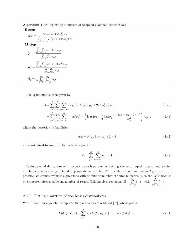
Algorithm 1 EM for fitting a mixture of wrapped Gaussian distributions

E step

ηijl =N(xi ; µj+2πl,σ2

j ) πjK∑j=1

∞∑l=−∞

N(xi ; µj+2πl,σ2j ) πj

M step

µj =

N∑i=1

∞∑l=−∞

(xi−2πl) ηijl

N∑i=1

∞∑l=−∞

ηijl

σ2j =

N∑i=1

∞∑l=−∞

(xi−µj−2πl)2 ηijl

N∑i=1

∞∑l=−∞

ηijl

πj = 1N

N∑i=1

∞∑l=−∞

ηijl

The Q function is then given by

Q =

N∑

i=1

K∑

j=1

∞∑

l=−∞

(log[πj N (xi ; µj + 2πl, σ2

j )])ηijl (2.40)

=

N∑

i=1

K∑

j=1

∞∑

l=−∞

(log(πj)−

1

2log(2π)− 1

2log(σ2

j )− (xi − µj − 2πl)2

2σ2j

)ηijl , (2.41)

where the posterior probabilities

ηijl = P (zjl | xi ; µj , σ2j , πj) (2.42)

are constrained to sum to 1 for each data point:

∀ iK∑

j=1

∞∑

l=−∞ηijl = 1 (2.43)

Taking partial derivatives with respect to each parameter, setting the result equal to zero, and solving

for the parameters, we get the M step update rules. The EM procedure is summarized in Algorithm 1. In

practice, we cannot evaluate expressions with an infinite number of terms numerically, so the WGs need to

be truncated after a sufficient number of terms. This involves replacing all∞∑

l=−∞(−) with

L∑l=−L

(−) .

2.3.3 Fitting a mixture of von Mises distributions

We will need an algorithm to update the parameters of a MovM [92], whose pdf is:

P (θ ; µ,κ,π) =

K∑

j=1

πj vM (θ ; µj , κj) , −π ≤ θ ≤ π . (2.44)

20

Algorithm 2 EM for fitting a mixture of von Mises distributions

E step

ηij =vM (θi ; µj ,κj) πjK∑j=1

vM (θi ; µj ,κj) πj

M step

µj = tan−1

N∑i=1

sin(θi) ηij

N∑i=1

cos(θi) ηij

A (κj) =I1(κj)I0(κj)

=

N∑i=1

cos(θi−µj) ηijN∑i=1

ηij

πj = 1N

N∑i=1

ηij

Because of the cos(−) term in the vM pdf, we will have to numerically update the concentration parameter

κ. The log likelihood is:

logL =

N∑

i=1

log

K∑

j=1

πj vM (θi ; µj , κj) , (2.45)

and the Q function is:

Q =

N∑

i=1

K∑

j=1

log [πj vM (θi ; µj , κj)] ηij (2.46)

=

N∑

i=1

K∑

j=1

[log(πj)− log(2π)− log(I0(κj)) + κj cos(θi − µj)] ηij , (2.47)

where the posterior probabilities

ηij = P (zj | θi ; µj , κj , πj) , (2.48)

are constrained to sum to 1 for each data point:

∀ iK∑

j=1

ηij = 1 . (2.49)

Taking partial derivatives with respect to each parameter and setting the results to zero gives the M step

update rules. The EM procedure is summarized in Algorithm 2. We can solve for κj with a zero-finder (e.g.

bisection search [88]) using the old estimate as a starting point.

21

2.3.4 Fitting a mixture of von Mises-Fisher distributions

Details about the EM algorithm for fitting a MovMF are discussed at length in [93]. There is also a k-means

algorithm for clustering on the sphere [94]. The pdf of a MovMF is given as:

P (x ; µ,κ,π) =

K∑

j=1

πj vMF (x ; µj , κj) , ‖x‖2 = 1 . (2.50)

The log likelihood is:

logL =

N∑

i=1

log

K∑

j=1

πj vMF (xi ; µj , κj) , (2.51)

and the Q function is:

Q =

N∑

i=1

K∑

j=1

log[πj vMF (xi ; µj , κj)

]ηij (2.52)

=

N∑

i=1

K∑

j=1

[log(πj) + log(κj)− log(2π)− log(eκj − e−κj ) + κjµ

Tj xi]ηij , (2.53)

where the posterior probabilities

ηij = P (zj | xi ; µ,κ,π) , (2.54)

are constrained to sum to 1 for each data point:

∀ iK∑

j=1

ηij = 1 . (2.55)

Taking partial derivatives, setting the results to zero and solving for the new parameters gives the M step

update rules. The EM procedure is summarized in Algorithm 3. The update of the concentration parameters

can be numerically unstable, but there are good approximations. For κ � 3, we can drop the e−κj terms

and use the following approximation [58]:

κj ≈1

1−A(κj). (2.56)

Even when the conditions for this approximation are not met, we find empirically that spherical data can

still be successfully clustered.

2.4 Interchannel phase difference features

We will use inter-channel phase differences (IPD) as a raw feature to perform multi-source separation and

tracking. The IPD representation is modified from that of [1] so as to incorporate spatial aliasing explicitly

in a statistical model. We show that these wrapped features compose a circular-linear dataset.

22

Algorithm 3 EM for fitting a mixture of von-Mises Fisher distributions

E Step

ηij =vMF (xi ; µj ,κj) πjK∑j=1

vMF (xi ; µj ,κj) πj

M step

µj =

N∑i=1

xi ηij

∥∥ N∑i=1

xi ηij

∥∥2

A (κj) = eκj+e−κj

eκj−e−κj −1κj

=

∥∥ N∑i=1

xi ηij

∥∥2

N∑i=1

ηij

πj = 1N

N∑i=1

ηij

2.4.1 Feature extraction

A microphone array with C channels captures C time-domain signals xi , i = 1, . . . , C. These signals are con-

verted to a time-frequency representation using the short-time Fourier transform (STFT) (see Section 2.1.1):

X(i) = STFT (xi) ∈ CD×T , (2.57)

where D denotes the coefficient index in the DFT corresponding to half the sampling rate. We ignore the

second half of the DFT because it contains the same information as the first half. Since the Fourier transform

is a linear operation, we have that the DFT coefficient at each time-frequency bin is approximately equal to

the sum of the contributions from the sources. In the absence of reverberation, this gives

X(i)f,t =

K∑

j=1

S(j)f,t · aij e−jωdij , ω =

πf

D, (2.58)

where S(j)f,t is the DFT coefficient of the jth source, aij and dij are the attenuation and delay for the direct

path between the ith microphone and the jth source, and ω is the digital frequency corresponding to the f th

frequency band.

We compute element-wise logratios to consolidate the STFT information across channels. For C = K = 2,

we have

Ff,t = log

(X

(1)f,t

X(2)f,t

)= log

(S

(1)f,t · a11e

−jωd11 + S(2)f,t · a12e

−jωd12

S(1)f,t · a21e−jωd21 + S

(2)f,t · a22e−jωd22

). (2.59)

If we assume that the signals are approximately disjoint in the STFT (see Equation (2.8)), then we can

simplify Equation (2.59) to the one-source case in each TF bin:

Ff,t ≈ log

(Sf,t · a1e

−jωd1

Sf,t · a2e−jωd2

)= log

(a1

a2

)− jω (d1 − d2) . (2.60)

The negative imaginary part of this logratio yields the IPD:

23

δf,t = − Im(Ff,t) = ω (d1 − d2) = ∠X(2)f,t − ∠X(1)

f,t , (2.61)

which is a (wrapped) linear function of frequency. For a fixed source position, we expect these features to

lie on a wrapped line in a plot of frequency vs. phase difference:

δf,t = ψ(α f) , α =π

D(d1 − d2) , (2.62)

where ψ(−) is the wrap mapping in Equation (2.15). To make the dependence on frequency explicit, we can

form the following IPD feature vector:

δf,t =[δf,t f

]. (2.63)

Now it is clear that a collection of these vectors composes a circular-linear dataset. The case of three or

more sources (K ≥ 3) is no different as long as the disjointness property (Equation (2.8)) holds for all source

pairs. For three or more microphones (C ≥ 3), the IPD feature vector contains C − 1 phase differences:

δf,t =[δf,t(1, 2) · · · δf,t(1, C) f

], (2.64)

where δf,t(1, i) is the phase difference calculated from the 1st and ith channels. This feature representation

is similar to that of MENUET [15].

2.4.2 Effect of reverberation on IPD features

The impact of reverberation on IPD features depends primarily on the physical arrangement of the array,

the sources, and other objects in the room. Consider a source signal s[n]. The recorded (reverby) signals are

x1[n] =

R∑

r=1

ar1 s[n− dr1] , x2[n] =

R∑

r=1

ar2 s[n− dr2] , (2.65)

where ari and dri are the attenuation and delay values for the rth reflection at the ith microphone. Now the

IPD features are given as

24

−3 −2 −1 0 1 2 3

50

100

150

200

250

300

350

400

450

500

IPD (simulated)

fre

qu

en

cy

Figure 2.8: Moderately distorted IPD plot for a synthetic, echoic recording of speech. Reflections off of thewalls in the (small) room cause sinusoid-like perturbations in the IPD line.

F = ∠STFT (x2)− ∠STFT (x1) (2.66)

= ∠

(R∑

r=1

S(ω)ar2e−jωdr2

)− ∠

(R∑

r=1

S(ω)ar1e−jωdr1

)(2.67)

= ∠

(R∑

r=1

S(ω)ar2 [cos(−ωdr2) + j sin(−ωdr2)]

)− ∠

(R∑

r=1

S(ω)ar1 [cos(−ωdr1) + j sin(−ωdr1)]

)(2.68)

= ∠

(R∑

r=1

S(ω)ar2 cos(ωdr2)− jR∑

r=1

S(ω)ar2 sin(ωdr2)

)− ∠

(R∑

r=1

S(ω)ar1 cos(ωdr1)− jR∑

r=1

S(ω)ar1 sin(ωdr1)

)

(2.69)

= tan−1

−

R∑r=1

S(ω)ar2 sin(ωdr2)

R∑r=1

S(ω)ar2 cos(ωdr2)

− tan−1

−

R∑r=1

S(ω)ar1 sin(ωdr1)

R∑r=1

S(ω)ar1 cos(ωdr1)

(2.70)

= tan−1

R∑r=1

ar1 sin(ωdr1)

R∑r=1

ar1 cos(ωdr1)

− tan−1

R∑r=1

ar2 sin(ωdr2)

R∑r=1

ar2 cos(ωdr2)

(2.71)

Thus, reverb results in a sinusoid-like wobble in the IPD data over frequency that depends very strongly

on the room characteristics and array/source positions. This is because the attenuations and delays are

heavily influenced by these factors. If the direct path has an attenuation coefficient that is much larger than

that of competing arrivals, that term dominates the argument of tan−1(−), which approximately reduces

25

Figure 2.9: IPD plot for synthetic mixture of three sources, colored according to likelihood probability. (Thisfigure appears in [20].)

to the case of no reverb, and the wobble is negligible. For extremely small rooms or otherwise in situations

with strong early reflections (e.g. off of an object holding the array), the non-linearity may be significant.

Figure 2.8 depicts a moderate case.

2.5 Circular-linear regression

A circular-linear dataset is one that contains vectors with two values: one linear and one circular [72]. That

is, one component describes a value that lies on the real line, R1, and the other describes a value that lies on

the unit circle, S1 (generalizations of this allow for more than two components). Circular-linear regression

is the problem of fitting a wrapped line2 to such a dataset. This is nothing but linear regression modulo 2π

in one of the variables.3 Each IPD feature vector corresponds to a TF bin, so we can form a binary mask

by partitioning the vectors by some clustering algorithm that fits multiple wrapped lines to the data. We

can view this as a multimodal circular-linear regression problem. We will see that source separation and

localization require only the slopes of the wrapped lines corresponding to the speakers.

26

2.5.1 IPDs as circular-linear data

An acoustic wavefront that arrives at a microphone array at an angle incurs a particular delay between

the microphones. By the delay property of the Fourier transform, this corresponds to a phase shift in the

frequency domain. More shift will exist at higher frequencies, resulting in data that lies along a wrapped

line. When multiple speakers are present and they are disjoint in the STFT, we observe data that traces

out multiple wrapped lines. An example of this for a synthetic, anechoic mixture of three sources captured

by a two-microphone array is shown in Figure 2.9. To perform IPD-based BSS, we will cluster the feature

vectors in Equation (2.63) and partition the mixture STFT accordingly. This is equivalent to the problem

of multimodal circular-linear regression, namely, recovering the underlying wrapped linear models.

2.5.2 Probabilistic model for circular-linear regression

Consider the case of fitting a single wrapped line of the form in Equation (2.62) to an IPD dataset ∆ = {δf,t}derived from a stereo recording. We can measure the goodness-of-fit of a wrapped line with slope α by a

likelihood criterion such as:

L(∆ ; α) =

D∏

f=1

T∏

t=1

P (δf,t ; ψ(αf), κ) , (2.72)

where the probability distribution is arbitrarily chosen to be vM for simplicity (we could also choose it to

be WG). Extending this to the case of multiple lines, we have:

L(∆ ; α) =

D∏

f=1

T∏

t=1

K∑

j=1

P (δf,t ; ψ(αjf), κ) . (2.73)

An example of multimodal circular-linear data generated from this model along with outliers sampled from

the uniform distribution is shown in Figure 2.10(a). The corresponding likelihood functions for three values

of the von Mises concentration parameter κ are shown in Figure 2.10(b). It is important to include the

uniform noise as IPD features tend to look this way in practice. Roughly half of the data in Figure 2.10(a)

can be considered outliers. Nevertheless, it is clear that peaks in the likelihood function correspond to the

slopes of the wrapped lines. For this dataset, a higher κ is necessary to differentiate the two lines with slopes

near 0.

2.6 Direction-of-arrival estimation

We will use 2-, 3-, and 4-microphone arrays to localize and track multiple speakers on the unit circle and

unit sphere. Thus, we will need a method to estimate the directions-of-arrival (DOA) of the sound sources.

2This has also been called a “barber pole regression curve” in the directional statistics literature [72] because it can bevisualized as a helix on the surface of a cylinder. A less intuitive but more general and correct interpretation would be thatIPD features in a single frequency band lie on a torus. The wrapped IPD lines are then visualized as spirals on a disk for thecase of 2 channels, where radius corresponds to frequency. Each concentric circle on the disk corresponds to a single frequencyband. For the case of three channels, IPD features lie on a torus (i.e. a donut) whose thickness changes with frequency.

3The case without spatial aliasing was discussed in [95].

27

−3 −2 −1 0 1 2 30

0.1

0.2

0.3

0.4

0.5

0.6

0.7

0.8

0.9

1

f

δ

(a)

9.459.5

9.559.6

k = 1

12.6

12.8

log

lik

elih

oo

d

k = 5

−1.5 −1 −0.5 0 0.5 1 1.5

106

106.5

k = 100

angle

(b)

Figure 2.10: (a) 10,000 data points showing several wrapped-line trends in the presence of outliers. (b) Loglikelihood as a function of DOA. The concentration parameter κ of the von Mises distribution determineshow strongly outliers are penalized.

Many methods exist for DOA estimation [9], [13], [22]. The most common technique is to search for peak(s)

in the inter-channel cross-correlation function over a grid in DOA space [26], [27]. When implemented with

a noise-shaping filter, this is called the generalized cross correlation (GCC) method [24], [25]. For localizing

multiple sources simultaneously, the steered response power (SRP) of a beamformer can be calculated over

DOA space. There are also well-known subspace methods like MUSIC [28] and ESPRIT [30] that use

eigendecompositions to identify signal and noise subspaces of the channel correlation matrix. In MUSIC,

a “pseudospectrum” is calculated that has peaks corresponding to the DOAs, and in ESPRIT, estimates

are calculated by solving a total least squares problem. Unfortunately, MUSIC requires at least as many

microphones as there are sources and ESPRIT requires at least twice as many.

In this thesis, we are concerned with estimating DOAs from inter-channel delays. The easiest approach is

to solve a least-squares problem to recover a direction vector [23]. Another method involves trigonometric

arguments. The only information we need for either is the relative positions of the microphones and an

estimate of the inter-channel delays. We review both of these in this section.

It will be important to relate the slope α of a wrapped line calculated from IPD data to the DOA of a

source. This can be done by first relating slopes to inter-channel delays. The slope α of a wrapped line is

related to the delay e12 (samples) from microphone 1 to microphone 2 by

α = − πDe12 . (2.74)

2.6.1 Least-squares DOA estimation

One method to solve for the DOA of a sound source reduces to solving a system of linear equations. We

can derive it by considering the physical arrangement of the microphones and the source. This is depicted

28

source

u(✓) m2

✓x

y

⌦

m3

v

s|e12|

v

s|e13|

Figure 2.11: Geometry of least-squares DOA estimation. The first microphone is located at the origin.

in Figure 2.11 for a 3-mic array in 2D space. The position of the ith microphone is

mi =[mi1 mi2

]T, (2.75)

and the vector connecting the ith and jth microphones is

qij = mi −mj . (2.76)

We denote a unit vector oriented in the direction θ as

u(θ) =[u1(θ) u2(θ)

]T, (2.77)

and note that an inner product relates this vector to the inter-channel delay eij for each mic pair:

qTiju(θ) =v

seij , (2.78)

where v is the speed of sound (meters sec−1) and s is the sampling rate (samples sec−1). This defines a

linear system of equations over all microphone pairs:

[q12 q13 q23

]Tu(θ) =

v

se , (2.79)

where the vector of delays is

e =[e12 e13 e23

]T. (2.80)

29

yt�1 yt+1yt

xt�1 xt xt+1

Figure 2.12: Graphical model of dynamic Bayesian network (DBN). The hidden state xt evolves over timeand emits an observed measurement yt. The goal of Bayesian filtering is to recursively infer the state fromonly the observation sequence y1:t and knowledge of the system dynamics.

Solving this system gives the least-squares solution for the source direction.

2.6.2 Trigonometric DOA estimation

We can also derive DOA estimators through trigonometric arguments. We start with the case of 1D localiza-

tion on a semicircle with 2 microphones. The angle of arrival θ can be related to the delay e12 and therefore

to the slope α as follows:

cos (θ) = −v∆t

d= − v

d se12 =

v D

π d sα , (2.81)

where v is the speed of sound (meters sec−1), D is the maximum frequency bin value, d is the distance

between the microphones (meters) and s is the sampling rate (samples sec−1). We can also derive DOA

estimators for localizing on the unit circle and hemisphere with 3 microphones and on the unit sphere with

4 microphones. These estimators are given in Appendix B.

2.7 Recursive Bayesian filtering

This section serves to summarize the Bayesian filtering framework for tracking the hidden state of a dynamical

system. We will use wrapped filters to track speakers on the unit circle and sphere. The DOA tracking

algorithms presented in this thesis require one or more observations (also called measurements) at each time

step. We can use raw IPD features from Section 2.4 as measurements or we can transform these features

into DOA estimates. This choice affects the system model. In this section, we review the basic approach to

Bayesian filtering for tracking one or more sources.

30

2.7.1 Bayesian filtering equations

The Bayesian filtering equations [38] describe the recursive inference procedure for dynamic Bayesian net-

works (DBN) [96], [97]. We will derive them here. The graphical model of the DBN is shown in Figure 2.12.

The (hidden) state xt evolves according to a transition distribution in Equation (2.82) and the observation

yt is emitted according to a measurement distribution in Equation (2.83):

xt ∼ P (xt |xt−1) , (2.82)

yt ∼ P (yt |xt) . (2.83)

The system dynamics are fully described by these two equations. Equivalently, we may use the notation:

xt = f (xt−1,vt) , (2.84)

yt = g (xt,wt) , (2.85)

where vt and wt are process and measurement noise variables with known statistics and the (possibly non-

linear) functions f(−) and g(−) dictate how the state and measurement are generated at time t. This

representation is often referred to as the state space model (SSM) of the system.

The filtered state distribution P (xt−1|y1:t−1) evolves according to two repeated steps, predict and correct,

that propagate it from time t−1 to time t. This density accumulates information about the entire observation

sequence y1:t−1 without explicitly storing its values. In the predict step, the filtered distribution is propagated

forward via (2.82):

P (xt|y1:t−1) =

∫P (xt,xt−1|y1:t−1) dxt−1 (2.86)

=

∫P (xt|xt−1,y1:t−1)P (xt−1|y1:t−1) dxt−1 (2.87)

=

∫P (xt|xt−1)P (xt−1|y1:t−1) dxt−1 . (2.88)

The prediction is then updated in the correct step via Equation (2.83):

P (xt|y1:t) = P (xt|yt,y1:t−1) (2.89)

=P (yt|xt,y1:t−1)P (xt|y1:t−1)

P (yt|y1:t−1)(2.90)

=P (yt|xt)P (xt|y1:t−1)

P (yt|y1:t−1)(2.91)

∝ P (yt|xt)P (xt|y1:t−1) . (2.92)

The resulting algorithm depends on the filtered, state transition, and observation densities. The Kalman

filter [33], [34] is optimal for a linear-Gaussian DBN. However, we will work with the WG, vM, vMF, and

mixtures of each one. Thus, the goal is to derive filters that approximate Equations (2.88) and (2.92) as

closely as possible.

31

Algorithm 4 Kalman filter

Predict

x−t = Axt−1

Σ−t = AΣt−1AT + Σv

Correct

Kt =Σ−t B

T

BΣ−t BT+Σw

xt = x−t +Kt

(yt −Bx−t

)

Σt = (I−KtB) Σ−t

2.7.2 Kalman filter

If the state space model (SSM) is linear-Gaussian:

xt = Axt−1 + vt , vt ∼ N (0,Σv) , (2.93)

yt = Bxt + wt , wt ∼ N (0,Σw) , (2.94)

where A and B are real-valued matrices, then the Bayesian filtering equations (2.88) and (2.92) can be solved

in closed form to yield the well-known Kalman filter [34]. The filtered state distribution P (xt|y1:t) remains

Gaussian from one time step to the next, so we need only estimate its mean xt and covariance Σt. The filter

equations can take various forms, one of which is given in Algorithm 4. The innovation term, yt − Bx−t , is

important because it captures how well the anticipated observation, Bx−t , matches the true observation, yt.

It also serves to inform the Kalman filter on how to adapt the state estimate to the new measurement.

Approximate Kalman filtering

Filtering schemes for a SSM that is not linear-Gaussian often involve a linear-Gaussian approximation of

the SSM. Although the Kalman filter is applicable to the new system, one must take care to account for the

inaccuracies introduced. The extended Kalman filter (EKF) [34] uses a first-order Taylor series expansion

to linearize non-linearities in the system dynamics. The unscented Kalman filter (UKF) [36], in contrast,

approximates the state distribution as a Gaussian and explicitly models the non-linearities via the unscented

transform [37]. A number of deterministically-chosen “sigma points” are calculated that capture the mean

and covariance of the filtered distribution. They are fed through the SSM to give transformed points that

are used to construct a Gaussian approximation of the filtered distribution in the next time step. It can

be shown that the UKF achieves a higher-order approximation and tends not to diverge in the presence of

strong non-linearities where the EKF does.

2.7.3 Particle filter

There are cases where the Bayesian filter equations cannot be approximated in some convenient closed

form. When all else fails, we can always attempt to represent the state distribution with a weighted set of

32

particles. These particles are propagated forward through time via the Bayesian filtering equations, which

involves sampling from the state transition distribution in Equation (2.82). If this distribution is difficult to

sample from, we can apply importance sampling techniques [87], [97].

Importance sampling

Suppose we would like to draw independent samples from a target distribution P (x), but we cannot do so

directly. We can side-step the issue by gathering samples, x(l), l = 1, . . . , L, from a suitably-chosen proposal

distribution Q(x) and assigning them weights:

w(l) ∝ P (x(l))

Q(x(l)). (2.95)

The importance weights compensate for any mismatch between P (x) and Q(x). We can assume that P (x)

(and even Q(x)) is known only up to a normalization constant. A well-matched proposal distribution will

ensure that the weights are spread near 1/L. If Q(x) is poorly-matched, many of the weights will be nearly

zero, giving bad results or an inefficient approximation scheme.

Sampling importance resampling

The samples x(l) ∼ Q(x) and their weights w(l) approximate the distribution P (x) as a weighted set of point

estimates. If we would like an unweighted sample set, we can resample by treating the weights vector w as

a categorical distribution. In other words, the new unweighted sample set consists of L i.i.d. draws from the

weighted approximation of P (x):

x ∼L∑

l=1

w(l) δ(x− x(l)

). (2.96)

One potential drawback is that heavily-weighted samples will be repeated, having been drawn with replace-

ment.

Sequential importance resampling (SIR)

The most straightforward technique for particle filtering is a repeated application of sampling importance

resampling to approximate the recursive scheme from Section 2.7.1. This is alternatively called sequential

importance resampling (SIR), bootstrap filtering, the condensation algorithm, and survival of the fittest.

Instead of keeping track of the entire state distribution in each time step, we approximate it with a set of

weighted Dirac deltas, referred to as particles. The filtered state distribution at time t− 1 is approximated

with a particle set

Xt−1 ={

x(l)t−1, w

(l)t−1

}, l = 1, . . . , L , (2.97)

by:

33

Algorithm 5 Particle filter - sequential importance resampling

Predict

x(l),−t ∼ P

(xt∣∣x(l)t−1

)

Correct

w(l),−t ∝ P

(yt∣∣x(l),−t

)w

(l)t−1

Resample

x(l)t ∼

L∑m=1

w(m),−t δ

(xt − x

(m),−t

)

w(l)t = 1

L

P (xt−1|y1:t−1) ≈L∑

l=1

w(l)t−1 δ

(xt−1 − x

(l)t−1

). (2.98)

When we propagate this particle set through the SSM in Equations (2.82) and (2.83) to the next time step,

we will have an updated particle set

Xt ={

x(l)t , w

(l)t

}, l = 1, . . . , L , (2.99)

that approximates the filtered distribution at time t:

P (xt|y1:t) ≈L∑

l=1

w(l)t δ

(xt − x

(l)t

). (2.100)

The set Xt is determined by combining Equation (2.98) and the Bayesian filtering Equations (2.88) and (2.92):

P (xt|y1:t) ∝ P (yt|xt)L∑

l=1

w(l)t−1 δ

(xt − x

(l),−t

)(2.101)

∝L∑

l=1

P(yt∣∣x(l),−t

)w

(l)t−1 δ

(xt − x

(l),−t

), (2.102)

where the predicted particles are sampled from the transition distribution:

x(l),−t ∼ P

(xt∣∣x(l)t−1

). (2.103)

Comparing Equations (2.100) and (2.102), we can say that the updated weights should be:

w(l),−t ∝ P

(yt∣∣x(l),−t

)w

(l)t−1 . (2.104)

The last step is to resample from the updated particle set to prevent degeneracy:

34

Xt�1 =nx

(l)t�1, w

(l)t�1

o

x(l),�t ⇠ P

⇣xt

�� x(l)t�1

⌘

P (yt | xt)

w(l),�t / P

⇣yt

�� x(l),�t

⌘w

(l)t�1

Xt =nx

(l)t , w

(l)t

o

Figure 2.13: Sequential importance resampling for particle filtering. Circles represent particles (size indicatesweight) and bars indicate the number of copies. (Top) Particle set at time t − 1 with four copies of each.(Top middle) Predict : propagate via transition distribution. (Middle) Meausurement likelihood. (Bottommiddle) Correct : re-weight via likelihood. (Bottom) Resample: sample i.i.d. from updated set.

x(l)t ∼

L∑

m=1

w(m),−t δ

(xt − x

(m),−t

)(2.105)

w(l)t =

1

L. (2.106)

The SIR procedure is depicted in Figure 2.13 and is summarized in Algorithm 5. To recap, we started at

time t−1 with a set of weighted particles and fed this through our SSM to get a sum-of-deltas approximation

of the posterior distribution at time t. Without resampling, the weights quickly degenerate (i.e. within a few

iterations) such that a single particle is left to represent the entire state distribution. In fact, it can be shown

that the variance of the weights increases exponentially with time [97]. Although many resampling techniques

exist including stratified sampling, systematic resampling, and Markov chain Monte Carlo methods, we will

35

use the multinomial resampling method described above.

SIR in context

SIR derives from a general formulation in which the new particles are sampled from a proposal distribution:

x(l)t ∼ Q(xt|xt−1,yt) , (2.107)

and the updated weights are given via importance sampling as:

w(l)t ∝ w(l)

t−1

P(x

(l)t

∣∣x(l)t−1

)P(yt∣∣x(l)t

)

Q(x

(l)t

∣∣x(l)t−1,yt

) . (2.108)

If we assume that the proposal is equal to the state transition distribution:

Q(x

(l)t

∣∣x(l)t−1,yt

)= P

(x

(l)t

∣∣x(l)t−1

), (2.109)

then the weight update reduces to that of the SIR algorithm. More clever proposals can improve the

accuracy of a particle filter when the state transition distribution and observation likelihood are very different.

However, we will only use the popular SIR algorithm in this thesis as it is conceptually simple, easy to

implement, and works quite well in practice.

Estimating statistics from a particle set

Statistics of the state distribution can be calculated from the particle set. This is best done before resam-

pling as it gives estimates with lower variance. For example, if the state distribution can be reasonably

approximated as a Gaussian, its mean and covariance can be estimated as:

xt =

L∑

l=1

w(l)t x

(l)t , (2.110)

Σt =

L∑

l=1

w(l)t

(x

(l)t − xt

)(x

(l)t − xt

)T. (2.111)

These may not always be appropriate statistics to evaluate. For example, if the SSM describes the evolution

of a system on the unit circle, we should calculate circular statistics instead.

2.7.4 Multi-source tracking with mixture models

In this thesis, we will derive algorithms for tracking K simultaneously active sources. We choose the state

space model to be a factorial DBN where multiple state chains xt,j , j = 1, . . . ,K evolve independently,

each of which produces an observation yt,j . However, we observe the unordered set of measurements yt =

{yt,m} , m = 1, . . . ,K:

36

∀ j xt,j ∼ P (xt,j |xt−1,j) (2.112)

∀ j yt,j ∼ P (yt,j |xt,j) (2.113)

yt = {yt,m} . (2.114)

A data association ambiguity exists because we do not know what observation was generated by what

source (i.e. the bipartite matching between j and m indices is hidden). Exact inference requires an

exponentially-growing model for the filtered state distribution. A well-known approximation is the switching

Kalman filter (SKF) [98], which collapses the filtered distribution in each time step such that its size remains

fixed.

We will model P (xt|y1:t) as a mixture and consider probabilistic assignments of observations/particles

to mixture components. These are incorporated as weights in the correct step of the filter, effectively

integrating out the unknown assignments. The reader is referred to the extensive literature on filtering with

mixtures [46], [47], [48] [66].

2.8 RANdom SAmple Consensus (RANSAC)

RANSAC is a hugely important method in the computer vision community for estimating a simple model

from a dataset with a large proportion of outliers [73]. If the model can be fully described by a small set

of points, then one simply needs to find such a set in the data to recover the parameters of the model. If

we wish to fit a line in R2, then only two points must be sampled. Each draw of a data pair is known as a

“RANSAC sample” and the line connecting them is known as a “candidate.” The number of inliers of each

candidate is calculated and the one with the most inliers is chosen as an estimate of the true model. Other

simple models such as circles and ellipses can also be found with RANSAC.

To ensure a good fit, a sufficiently high number M of candidates is collected. This is given by the expected

number of trials E[t] until an inlier is chosen. If the proportion of inliers in the dataset is p and we need to

sample n data points to fit a model, it can be shown that E[t] = p−n. In practice, M is overestimated to

ensure a good fit. A final detail is that we must specify an inlier criterion (typically a thresholded distance

function). The overall procedure is summarized in Algorithm 6.

RANSAC has a marked advantage for line-fitting in the presence of outliers compared to standard linear

regression by least-squares. Consider the dataset in Figure 2.14 in which half of the data are sampled

uniformly at random and half are sampled from a line with Gaussian-distributed error. Standard linear

regression is thrown off by the outliers, whereas RANSAC completely ignores them. This is because a

candidate line not aligned with the inlier set receives far fewer votes than one that is.

In this thesis, we are interested in fitting a wrapped line that passes through the origin in IPD space.

Thus, we only need one point to fully specify the model. Because of this, a RANSAC-based approach will

be very fast and robust to the effects of unknown interference and reverberation.

37

Algorithm 6 RANSAC

Inputs: X = {xi} : N data points

Outputs: α : parameter estimates

Y = M RANSAC samples drawn uniformly at random from X

I = 0N×M

for m = 1 : M do

Fit model with parameters αm to Ym

I(i,m) = 1 , ∀i s.t. xi is inlier of mth model

end for

m = argmaxm

∑i

I(i,m)

return αm

datatrueLSRANSAC

Figure 2.14: Line-fitting in uniform noise with least-squares regression (LS) and RANSAC. Half the dataconsists of outliers chosen uniformly at random in the square.

38

CHAPTER 3

BSS AND DOA ESTIMATION FOR MULTIPLE STATIONARY

SPEAKERS

This chapter discusses algorithms for blind source separation (BSS) and direction-of-arrival (DOA) estimation

of multiple, physically stationary speakers using wrapped IPD features. The basic idea is to cluster the

features (see Section 2.4) according to a probabilistic circular-linear model. This takes spatial aliasing into

account and does away with a permutation ambiguity across frequencies [4].1 Two clustering methods are

proposed: one uses EM and the other uses a sequential variant of RANSAC [73]. The latter is shown to be

more efficient and accurate. It is also shown that the results of the clustering provide an estimator of the

DOAs of the speakers. We will use this fact in Chapter 4 to track moving speakers over time.

3.1 EM for fitting a mixture of wrapped lines

The source separation problem can be reduced to one of multimodal circular-linear regression (see Sec-

tion 2.5). It is instructive to view this as a parameter estimation problem with latent variables. Then, we

can apply the Expectation-Maximization (EM) framework (see Section 2.3.1). The observed variables are

the IPD data, the hidden variables are the TF bin labels (i.e. which source is active), and the unknown

parameters are the IPD line slopes (or, equivalently, the source DOAs). The well-known graphical model for

this sort of clustering problem is shown in Figure 3.1. We first consider the approach in a single frequency

band and then extend this to combine information across frequencies.

3.1.1 Clustering in each frequency band individually

Consider the IPD clustering problem in a single frequency band. The observation model consists of a mixture

of wrapped distributions on the interval [−π, π], one for each source. The generative process involves choosing

one component from the mixture with some probability and sampling a data point from that distribution.

This is repeated until N i.i.d. samples are collected. Having observed this data, we would like to discover

the parameters of the underlying mixture.

We can model each source distribution as a wrapped Gaussian (WG) and run the EM algorithm to fit

a MoWG (see Section 2.3). The posterior probabilities from EM indicate how to construct a binary mask.

However, clustering in each frequency band individually fails to capture the wrapped linear structure of

the IPD lines. This results in a permutation ambiguity [100] where it is unclear how to group the clusters

1A related approach called Model-based Expectation-maximization Source Separation and Localization (MESSL) incorpo-rates IPDs and inter-channel level differences (ILD) [99]. However, in real-world scenarios with compact arrays, ILD featurestypically provide little to no information and may significantly reduce performance.

39

�

z

↵

�2

⇡

T

Figure 3.1: Graphical model for wrapped-line fitting. Observed IPD vectors y are generated by samplingfrom a mixture of wrapped lines with parameters {α,σ2,π}. Hidden variables z associate each TF bin witha line.

across frequencies such that each group contains the WGs corresponding to a single source (this is a famous

problem for ICA-based BSS [4]). In the next section, we modify this approach to perform the clustering

jointly across all frequencies.

3.1.2 Clustering across frequencies

To incorporate the linear trend of IPD data across frequency, we reparameterize the model from the previous

section in terms of the slopes αj :

µjf = αjf . (3.1)

This locks the means together for each line, resulting in what appears to be a multivariate WG. However,

the pdf this distribution does not factorize into a product of densities, but is modeled as a sum of univariate

WGs. This is because the frequency bands are completely separated in the generative model. We call this

separated, wrapped, and mean-locked distribution a multi-band wrapped Gaussian (MWG).

The EM algorithm to learn a mixture of MWGs (MoMWG) proceeds as follows. We have a dataset of T

vectors ∆ = {δt}, δt ∈ ST×1, sampled i.i.d. from a mixture of multi-band wrapped Gaussians. The pdf of

this distribution is

P (δ ; α,σ2,π) =

K∑

j=1

πj

D∑

f=1

1

D

∞∑

l=−∞N (δf ; αjf + 2πl , σ2

jf ) , (3.2)

the log likelihood function for parameter estimation is

log L ∝T∑

t=1

log

K∑

j=1

D∑

f=1

∞∑

l=−∞πj N

(δf,t ; αjf + 2πl , σ2

jf

), (3.3)

and the Q function is

40

Algorithm 7 EM for fitting a mixture of multi-band wrapped Gaussian distributions

E step

ηtjfl =N(δf,t ; αjf+2πl , σ2

jf) πjK∑j=1

D∑f=1

∞∑l=−∞

N(δf,t ; αjf+2πl , σ2jf) πj

M step

αj =

T∑t=1

D∑f=1

∞∑l=−∞

f (δf,t−2πl)σ2jf

ηtjfl

T∑t=1

D∑f=1

∞∑l=−∞

f2

σ2jf

ηtjfl

σ2jf =

T∑t=1

∞∑l=−∞

(δf,t−αjf−2πl)2 ηtjfl

T∑t=1

∞∑l=−∞

ηtjfl

πj = 1T

T∑t=1

D∑f=1

∞∑l=−∞

ηtjfl

Q =

T∑

t=1

K∑

j=1

D∑

f=1

∞∑

l=−∞

(log[πj N (δf,t ; αjf + 2πl , σ2

jf )])ηtjfl (3.4)

=

T∑

t=1

K∑

j=1

D∑

f=1

∞∑

l=−∞

(log(πj)−

1

2log(2π)− 1

2log(σ2

jf )− (δf,t − αjf − 2πl)2

2σ2jf

)ηtjfl . (3.5)

The posterior probabilities

ηtjfl = P (zj,l | δf,t ; αj , σ2jf , πj) , (3.6)

are constrained to sum to 1 for each (multivariate) data point:

∀ tK∑

j=1

D∑

f=1

∞∑

l=−∞ηtjfl = 1 . (3.7)

A standard derivation leads to the EM equations summarized in Algorithm 7. To avoid over-fitting, we

can further constrain the model to have one variance parameter for each band or for the entire mixture (i.e.

a scalar). This simply adds summations to the numerator and denominator of the variance update rule.

3.1.3 Drawbacks of EM

The issues with the EM algorithm for this problem are three-fold. First, this approach is slow. A 4-D array

of posterior probabilities must be calculated in each E step. Second, this method is complicated relative

to the inherent simplicity of the problem. The main complication arises from the wrapping of the linear

models. However, this intuitively should not cause a large increase in algorithm complexity. And third, the

wrapping and noisy nature of IPD data leads to the existence of many local maxima in the log likelihood.

41

Algorithm 8 Sequential RANSAC for fitting multiple wrapped lines

Inputs: ∆ = {δi} : N IPD data points

K : number of wrapped lines to fit

Outputs: α = {αj} : K slopes

Y = M samples from ∆ selected uniformly at random

I = 0N×M

for m = 1 : M do

Fit line with slope αm to Ym

I(i,m) = 1 , ∀i s.t. δi is inlier of line with slope αm

end for

α = {}A = {1, . . . , N}for j = 1 : K do

m = argmaxm

∑i∈A

I(i,m)

α = α ∪ αmA = A \ {i : I(i, m) = 1}

end for

return α

Since EM performs a local optimization, it may converge to a solution that does not correspond to the true

source DOAs.

However, this approach has the advantage of explicitly modeling the wrapped nature of the data. We can

expect a good model to be fit as long as the initial conditions are sufficiently close to the correct solution.

In the next section, we present a much faster heuristic method to perform the clustering.

3.2 Circular-linear regression by random sampling

We describe a fast method for clustering IPD data based on the RANdom SAmple Consensus (RANSAC)

algorithm. RANSAC [73] was introduced in Section 2.8. We summarize a sequential approach [20] to fit

multiple wrapped lines to a circular-linear dataset.

3.2.1 Sequential RANSAC

Multi-model variants of RANSAC have been proposed for stereo imaging applications [101], [102], [103].

As discussed in [20], we can apply a sequential approach to cluster IPD data efficiently and robustly. The

generative model involves sampling i.i.d. from a mixture of multi-band wrapped distributions. We arbi-

trarily choose the von Mises distribution in this context for its simplicity. The procedure is summarized in

Algorithm 8, where the data is indexed by i rather than the pair {f, t} for clarity. M is scaled proportionally

with the number of sources K.

Consider the following example. Figure 3.2(a) shows the IPD data for an anechoic mixture of two TSP

42

(a) (b) (c)

Figure 3.2: Example of sequential RANSAC for wrapped line-fitting. (a) IPD data with 5 RANSAC samplesoverlaid. (b) First iteration of sequential RANSAC showing candidate wrapped lines and their inlier counts.(c) Second iteration of sequential RANSAC after removal of the inliers of the first model.

Figure 3.3: IPD plot of highly reverberant (T60 = 1.5 seconds), 2-speaker stairwell recording with wrappedlines fit by sequential RANSAC overlaid. Sequential RANSAC succeeds despite the fact that 65% of thedata consists of outliers. (This figure appears in [20].)

speakers. Five RANSAC samples have been chosen uniformly at random. Figure 3.2(b) shows the corre-

sponding wrapped line candidates and their inlier counts. The orange line is chosen and removed along with

its inliers. This process is repeated to find the next best candidate, the yellow line, as shown in Figure 3.2(c).

3.2.2 Why sequential RANSAC works

We have found that sequential RANSAC as applied to the IPD line fitting problem works very well for

a wide range of conditions. In [20], the example was given of a stereo recording in a stairwell whose T60

reverberation time was 1.5 seconds. The IPD plot for this recording is shown in Figure 3.3. Roughly 65%

of the data consists of outliers, yet the line-fitting is still successful. We can understand this by considering

the original probabilistic model for circular-linear regression presented in Section 2.5.2.

When RANSAC samples are drawn from the dataset ∆, they are effectively sampled from the likelihood

43

function shown in Figure 2.10(b).2 We expect to draw more candidates from high-density regions in the

likelihood function, so it makes intuitive sense that relatively few samples are required to fit the IPD lines.

The speed and simplicity of sequential RANSAC make it the author’s method of choice for clustering noisy,

wrapped IPD data.

3.3 Blind source separation and DOA estimation

We will now see how the BSS and DOA estimation problems can be solved with sequential RANSAC.

3.3.1 Blind source separation

We review the BSS method proposed in [20] for the stereo unmixing case and elaborate on how this is

extended to handle 3 or more microphones. Phase differences are calculated according to Equation (2.63),

resulting in a dataset ∆ = {δf,t}. Sequential RANSAC is then applied to fit K wrapped lines to this data.

The (f, t)th data point is considered an inlier of the jth line if δf,t is within ±π8 of the mean µjf = ψ(αjf).

This is equivalent to the criterion:

cos(δf,t − µjf ) ≥ cos(π

8

). (3.8)

To recover the K source signals, we apply time-frequency (TF) masks to one of the mixture STFTs and

apply the inverse STFT (see Section 2.1.1). The mask weights are given by the posterior probabilities:

wftj =P (δf,t ; µjf , κ)K∑j=1

P (δf,t ; µjf , κ)

=eκ cos(δf,t−αjf)

K∑j=1

eκ cos(δf,t−αjf)

. (3.9)

This probability represents the soft assignment of the (f, t)th bin to the jth source. Increasing κ results

in a more aggressive separation. In the limit as κ → ∞, Equation (3.9) reduces to a maximum-likelihood

binary mask where each bin contributes to the reconstruction of only one source:

∀ f, t wbftj =

1 if wftj = maxl

wftl

0 else. (3.10)

We can extend the IPD feature vectors as in Equation (2.64) to take advantage of additional mics. The

higher-dimensional data has multiple circular variables, increasing the inter-cluster distances. This leads to a

better clustering and, therefore, separation. We calculate inliers by expanding the criterion in Equation (3.8):

C−1∑

i=1

cos(δf,t(1, i+ 1)− µjfi) ≥ (C − 1) cos(π

8

), (3.11)

2Actually, this is not correct because multiple wrapped lines can pass through any data point. We can compensate by onlysampling from low-frequency data. This is acceptable for speech separation since the most reliable TF bins are in this range.High-frequency bins are more noisy but still help to validate the fitting.

44

where µjfi = ψ (αijf) is the value of the jth wrapped line in the f th frequency band and ith circular axis.

αij denotes the jth slope in the ith circular axis. This criterion implicitly assumes that regression error is

measured with a multivariate von Mises (vM) distribution [104] whose dimensions are independent. The

mask weights are also generalized via the multivariate vM:

wftj =P (δf,t ; µjf , κ)K∑j=1

P (δf,t ; µjf , κ)

=

C−1∏i=1

eκ cos(δf,t(1,i+1)−αijf)

K∑j=1

C−1∏i=1

eκ cos(δf,t(1,i+1)−αijf)

. (3.12)

3.3.2 Direction-of-arrival estimation

We can use sequential RANSAC to estimate the directions-of-arrival (DOAs) of multiple sound sources in a

reverberant environment. Sequential RANSAC is run on an IPD dataset to estimate a set of wrapped lines.

The slopes of the IPD lines are converted to inter-channel delays according to Equation (2.74). Finally,

a DOA estimator from Section 2.6 can then be used to convert these delays into estimates of the source

directions.

Least squares vs trigonometry

The two DOA estimators presented in Section 2.6 give essentially identical answers with non-degenerate

arrays. However, in certain cases, such as localization on a hemisphere with 3 or more coplanar mics, the

least-squares method requires the inversion of a rank-deficient matrix. This is remedied by first solving a

rank-2 LS problem for the source direction within the plane of the array and then solving for the missing

component perpendicular to the plane.

3.4 Experiments

In this section, we describe several experiments with blind source separation and DOA estimation for the

case of stationary speakers.

3.4.1 Synthetic multimodal circular-linear data

We first investigate the performance of sequential RANSAC. Synthetic data was generated from a mixture

of wrapped lines with moderate noise and uniform mixing weights. The slopes α were sampled such that

the corresponding DOAs θ were uniform in the range [−π2 , π2 ] with the condition that the angles differ by at

least π32 . The linear variable ranges from 0 to 1 and the circular variable ranges from −π to π. At most 3

full wrap-arounds were allowed. To test the robustness of the method to outliers, a portion of the data was

sampled uniformly at random over the circular variable. Data points are counted as inliers if they are within

±π8 of the line.3 During the fitting, all lines with slopes in the range [−6π, 6π] that passed through a point

were considered. This is necessary in the general case because multiple lines can be fit to a single sample.

3This is equivalent to the vM likelihood criterion: P (δ ; µ , κ) > 12P (µ ; µ , κ), µ = ψ(αf), κ = 9.1.

45

Table 3.1: Accuracy scores for sequential RANSAC with synthetic mixtures of K wrapped lines. A scoreabove 75 indicates a nearly perfect fit (shaded in gray).

K \% outliers 0 20 40 60 801 96.18 96.58 96.98 96.47 95.722 93.90 92.81 92.63 93.18 85.393 90.70 90.11 88.09 84.00 61.984 86.96 84.84 82.48 72.61 33.705 83.03 79.62 72.51 53.41 20.14

Figure 3.4: Models fit by sequential RANSAC. The red lines are the ground truth and the blue lines areinferred. (Far left) K = 1, % outliers = 80. (Middle left) K = 3, % outliers = 40. (Middle right) K = 5, %outliers = 40. (Far right) K = 5, % outliers = 80.

To quantify performance, a mixture of Laplacian distributions with scale parameter b = 0.2 and location

parameters set to the true DOAs θ was constructed. The following ratio of likelihoods was evaluated to

generate an accuracy score between 0 and 100:

A(φ ; θ , b) = 100P (φ ; θ , b)

P (θ ; θ , b)= 100

K∏i=1

K∑j=1

e−|φi−θj |

b

K∏i=1

K∑j=1

e−|θi−θj |

b

, (3.13)

where φi is the ith DOA found by sequential RANSAC. This accuracy function captures the peaked nature of

the underlying likelihood surface shown in Figure 2.10(b) and so can be considered an appropriate measure

of success. Inspecting the results, one can say that an accuracy score above 75 indicates an excellent fit.

100 trials were run for each model order-% outliers pair and 1000 data points were generated in each trial

from a new mixture of wrapped lines. The average accuracy scores for these toy experiments are summarized

in Table 3.1. Figure 3.4 shows examples of estimates returned by sequential RANSAC. It does an excellent

job of inferring the wrapped lines in the presence of many outliers.

3.4.2 Blind source separation

To test sequential RANSAC’s viability for BSS, we simulated a reverberant room with an array of omnidi-

rectional microphones placed at its center. We mixed two-second sentences by five speakers from the TSP

corpus [81]. They were positioned at random, distinct angles on the unit semicircle, circle, and sphere for 2-,

3-, and 4-channel unmixing. The microphones were positioned 5 cm apart in a right-angle configuration. We

46

Figure 3.5: Signal-to-distortion, signal-to-interference, and signal-to-artifact ratios for 2- and 3-channelsource separation in a 2D room and 4-channel source separation in a 3D room. C is the number of channelsand K is the number of sources. (Figure appears in [20].)

ran 100 trials for K = {2, 3, 4, 5} speakers with sentences downsampled to 16 kHz. STFTs were calculated

with a window size of 1024 and an overlap factor of 34 .

We simulated reverberation with the image method [23], [105], with the T60 time4 of the room varying

from 0 to 308 milliseconds. We used a 2D room (5 × 5 m) for testing 2- and 3-channel separation and a

3D room (5× 5× 5 m) for testing 4-channel separation. We evaluated the separation performance with the

BSS Eval toolbox [21]. This requires that we provide reference signals for each speaker. Because we are

testing for source separation and not de-reverberation, the reference is chosen to be the convolution of the

individual speaker signals with the appropriate room impulse responses. De-reverberation can be viewed as

a post-processing step.

Figure 3.5 summarizes the performance with a binary mask. We can see that, in general, the separation

quality improves with more microphones. However, there is a decrease in performance from the 2D to

the 3D rooms. This is due to the increased amount of reverberation. Because speech signals are quite

sparse, the loudest 10-20% of the TF bins should be used for clustering. Figure 3.3 depicts the fitting for a

highly-reverberant, real-world case with two male speakers in a stairwell. Despite a T60 time of 1.5 seconds,

sequential RANSAC succeeds in fitting the correct wrapped lines. A subjective assessment of the output

confirmed that the speakers were mostly separated. This is remarkable given how harsh the conditions are

for separation (and localization).

3.4.3 Direction-of-arrival estimation

Direction-of-arrival estimation in the context of sequential RANSAC is no more difficult than the source

separation problem. This is due to the simple mapping from DOA to IPD line slopes (see Section 2.6). In

other words, both the BSS and DOA estimation problems are solved simultaneously by sequential RANSAC.

A likelihood surface over the DOA space can be calculated from Equation (2.72) via the mapping. This

surface very closely resembles the histogram of inliers calculated by RANSAC. An example of this for DOA

estimation on the unit sphere in an anechoic 3D room with a 4-microphone array is shown in Figure 3.6(a).

4The T60 time of a room is the time required for the reverberation energy to drop by 60 dB below the direct path energy.

47

(a) (b)

Figure 3.6: Likelihood surfaces for synthetic DOA estimation with 4 sources and a 4-microphone array. Thespeakers recite TSP sentences 2.5 seconds long. Every azimuth-zenith pair corresponds to a DOA on theunit sphere. Sequential RANSAC is successful in identifying the speaker directions (marked with red *’s).(a) Anechoic conditions. (b) Reverberant conditions with T60 = 0.3 seconds.

Reverberation reduces the sharpness of the surface, as shown in Figure 3.6(b), but even in these conditions,

the sources are still located accurately.

The likelihood for a more complicated example with 6 sources is depicted in Figure 3.7 at each iteration of

sequential RANSAC. We can see that each peak corresponds to a speaker direction and that the algorithm

is able to successfully remove them one by one without propagating significant errors from one iteration to

the next. It is interesting to note that the localization is accomplished just by random sampling from the

dataset. This is much faster than scanning over all of DOA space, as is done in steered response power (SRP)

methods [13]. We also observe that no TF bin selectivity was applied in calculating the likelihood surfaces.

We can expect the peaks to be much more salient if only the TF bins with significant speech energy are

fed to sequential RANSAC. This requires a pre-processing step that could, for example, find peaks in the

magnitude STFT corresponding to the harmonics of speech [23].

3.4.4 Comparison with Bartlett beamformer and MUSIC

In this section, we compare the steered response power (SRP) of the Bartlett beamformer [13], the MUSIC

pseudospectrum [28], and the IPD likelihood function. The Bartlett beamformer measures how much power

is present at each DOA, frequency, and time by computing the following SRP function:

Pf,t(θ) = |ςf (θ)H Xf,t|2 , (3.14)

where

48

Xf,t =[X

(1)f,t · · · X

(C)f,t

]T, (3.15)

is the vector of DFT coefficients from all the channels and

ςf (θ) =[1 e−j

2πfN e12 · · · e−j

2πfN e1C

]T, (3.16)

is known as the “steering vector.” It encodes the phase information that we expect to see for a signal arriving

at frequency f and DOA θ and depends on the inter-channel delays e1i , i = 1, . . . , C. Accumulating over

all time-frequency bins gives the SRP for the Bartlett beamformer:

P (θ) =

T∑

t=1

D∑

f=1

Pf,t(θ) . (3.17)

This is equivalent to scanning DOA space with a delay-and-sum beamformer. We apply the PHAse Trans-

form [24] (PHAT) to the inputs before calculating the SRP. This involves setting all the magnitudes of the

DFT coefficients to 1, improving the response function by retaining only phase information.

The MUSIC spectrum is given by

Rf,t(θ) =1

C∑j=2

|ςHf (θ)b(j)f,t|2

, (3.18)

where b(j)f,t is the jth eigenvector of the spatial correlation matrix:

Σf,t = E[Xf,t XH

f,t

]= Bf,t Λf,t BH

f,t , (3.19)

Bf,t =[b

(1)f,t · · · b

(C)f,t

], Λf,t = diag

([λ

(1)f,t · · · λ

(C)f,t

]), (3.20)

and the eigenvalues are sorted in non-ascending order. Under additive white-noise assumptions, peaks will

be present in the accumulated MUSIC spectrum:

R(θ) =

T∑

t=1

D∑

f=1

Rf,t(θ) . (3.21)

We can compare the functions P (θ) and R(θ) with the von Mises (vM) likelihood in Equation (2.72)

over DOA space. A hard-thresholded alternative is calculated by accepting features within some distance of

the IPD line. Figure 3.8 shows these functions for a 3-mic array arranged in an equilateral triangle with 3

centimeters of spacing. Three TSP speakers are located at θ = −π3 , 0, π3 . The vM concentration and inlier

threshold are set to {1000, π16} and {100,π8 } for the anechoic and echoic cases. The T60 time for the echoic

case is 30 milliseconds. The IPD likelihood surface retains its peaks in a reverberant environment while the

MUSIC spectrum does not. It also requires fewer computations since no eigendecompositions are needed.

The SRP-PHAT function, on the other hand, can only be used to estimate two of the speakers’ locations.

49

Figure 3.7: Likelihood surfaces for 4-microphone localization of 6 speakers in anechoic conditions. SequentialRANSAC is able to incrementally identify the DOAs of all 6 speakers by, in effect, sampling from thelikelihood surface and removing inliers. The figures are ordered downwards with the left column first.

50

−π −2 π / 3 −π / 3 0 π / 3 2 π / 3 π

2006

2008

log L

IPD−soft

−π −2 π / 3 −π / 3 0 π / 3 2 π / 3 π

5101520

inliers

IPD−hardx 10

3

−π −2 π / 3 −π / 3 0 π / 3 2 π / 3 π1.25

1.3

log P

(θ)

SRP−PHATx 10

1

−π −2 π / 3 −π / 3 0 π / 3 2 π / 3 π

1.65

1.7

log R

(θ)

MUSICx 10

1

DOA

−π −2 π / 3 −π / 3 0 π / 3 2 π / 3 π

207.5

208

208.5

log L

IPD−soft

−π −2 π / 3 −π / 3 0 π / 3 2 π / 3 π

1

1.5

2

inliers

IPD−hardx 10

4

−π −2 π / 3 −π / 3 0 π / 3 2 π / 3 π

1.28

1.3

log P

(θ)

SRP−PHATx 10

1

−π −2 π / 3 −π / 3 0 π / 3 2 π / 3 π

1.6651.67

1.675

log R

(θ)

MUSICx 10

1

DOA

Figure 3.8: SRP-PHAT response power, MUSIC spectrum, and IPD likelihood for a simulated, 3-microphone,3-speaker experiment. Dashed lines indicate the source positions. (Left) Anechoic conditions. (Right) Echoicconditions. The T60 reverberation time is 30 milliseconds and the room dimensions are 5 × 5 meters. Thepeaks corresponding to the speakers can be seen under both conditions only in the IPD-based function.

51

CHAPTER 4

DIRECTION-OF-ARRIVAL TRACKING WITH IPD FEATURES

In the previous chapter, we saw how IPD features can be clustered to perform source separation and local-

ization. However, it was assumed that the speakers were physically stationary. This is often not the case in

a real-world environment. If we allow the speakers to move, the IPD line slopes become dependent on time.

This can be more appropriately expressed as a tracking problem in direction-of-arrival (DOA) space. If we

are given the sources’ DOA paths over time, the separation problem reduces to that of the previous chapter.

Thus, we will focus solely on the problem of multiple DOA tracking.

We will apply Bayesian filtering techniques to estimate the unobserved DOA paths (see Section 2.7 for

an overview). The observation can be DOA votes calculated by applying sequential RANSAC to a few

STFT frames worth of IPD data or the raw IPD features themselves. In either case, we will use directional

distributions to track speakers directly on the unit circle and sphere (see Section 2.2 for a review of directional

statistics). The Kalman filter is modified to handle tracking on the unit circle, S1, by modeling the state

distribution of a wrapped dynamical system with a wrapped Gaussian (WG). This new algorithm is called

the wrapped Kalman filter (WKF). A mixture of WGs is then used to track multiple sources on S1 with the

factorial WKF (FWKF). We will see that the WKF and FWKF can be interpreted as good approximations

of switching Kalman filter [98] procedures.

The von Mises-Fisher (vMF) distribution is then used to model the state distribution of a spherical

dynamical system. The tracking is performed with a von Mises-Fisher particle filter (vMFPF) [61]. Finally,

this is expanded to the multiple-source case with a mixture of vMFs to yield the factorial von Mises-Fisher

particle filter (FvMFPF). When multiple speakers are present, there is a data association ambiguity because

we do not know what state generated what observation (see Section 2.7.4 for a summary of the problem). To

remedy this, we will incorporate posterior probabilities into the filter equations that capture the probabilistic

assignments of observations to source clusters.

4.1 Bayesian tracking on the unit circle

We now describe algorithms for tracking directly on the unit circle with the wrapped Gaussian (WG)

distribution. The WG contains an infinite sum of periodic Gaussians, so the filtered state distribution

can only be approximated as WG from one time to the next. However, for low to moderate noise levels, this

is acceptable.

52

4.1.1 State space models for wrapped filtering

In this section, we present two dynamical systems that model the evolution of a circular state variable: a

rotating vector model and the wrapped dynamical system.

Rotating vector model

The following rotating-vector state space model [54] is often used for filtering with circular data:

xt =

[1 dt

0 1

]xt−1 + vt , vt ∼ N

(0,

[σ2v,1 0

0 σ2v,2

])(4.1)

yt =

[cos(xt,1)

sin(xt,1)

]+ wt , wt ∼ N

(0, σ2

wI). (4.2)

The state vector xt ∈ R2 consists of position and velocity, yt ∈ R2 is the observation vector, dt is the time

increment, and vt ∈ R2 and wt ∈ R2 are the process and measurement noise, respectively. The measurement

in Equation (4.2) involves a non-linear transformation of the state. The extended Kalman filter (EKF) [54]

approximates this by a first-order linearization, whereas the unscented Kalman filter (UKF) [55] does so

with the unscented transform.

The drawback of this model is that it regards the observation as a 2D vector when the state is truly

1D (and can be inferred via ∠yt). This introduces additional noise to the system that limits the tracking

capabilities of the filters. Contours of the distribution of yt are shown in the top panel of Figure 2.5.

Wrapped dynamical system

The wrapped dynamical system (WDS) is described by the following state space model:

θt = ψ (θt−1 + vt) , vt ∼ N(0, σ2

v

)(4.3)

yt = ψ (θt + wt) , wt ∼ N (0, σ2w) (4.4)

where θt, yt ∈ S1 and vt, wt ∈ R1. The wrapping in the state space is not crucial to the operation of the

WKF, but we include it here (in the generative model) for completeness. Additional state information can

easily be included by extending the state vector as it is done in the traditional Kalman filter since these

quantities are not wrapped and do not appear in Equation (4.4). For simplicity, we will only consider position

in the derivation of the WKF. A typical sample path for the WDS is shown in Figure 4.1 along with an

observation sequence and the state path estimated by the WKF.

The advantage of the WDS over the rotating vector model is that the observations are treated as 1D

quantities. We can expect that filtering in this model will be more accurate since it is easier to infer the

hidden state sequence θ1:T from lower-dimensional measurements. This fact is used to reduce the variance of

particle filtering schemes and is mathematically formalized in the Rao-Blackwell theorem [39]. Conceptually,

the WDS is an application of this approach to the rotating vector model in which the radius of yt in

Equation (4.2) is marginalized out (see top panel of Figure 2.5).

53

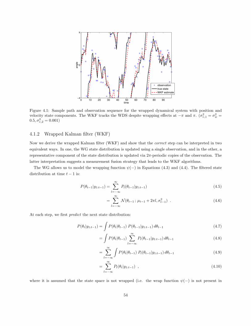
0 10 20 30 40 50 60 70 80 90time

an

gle

−π

0

π

observation

true state

WKF estimate

Figure 4.1: Sample path and observation sequence for the wrapped dynamical system with position andvelocity state components. The WKF tracks the WDS despite wrapping effects at −π and π. (σ2

v,1 = σ2w =

0.5, σ2v,2 = 0.001)

4.1.2 Wrapped Kalman filter (WKF)

Now we derive the wrapped Kalman filter (WKF) and show that the correct step can be interpreted in two

equivalent ways. In one, the WG state distribution is updated using a single observation, and in the other, a

representative component of the state distribution is updated via 2π-periodic copies of the observation. The

latter interpretation suggests a measurement fusion strategy that leads to the WKF algorithms.

The WG allows us to model the wrapping function ψ(−) in Equations (4.3) and (4.4). The filtered state

distribution at time t− 1 is:

P (θt−1|y1:t−1) =

∞∑

l=−∞Pl(θt−1|y1:t−1) (4.5)

=

∞∑

l=−∞N (θt−1 ; µt−1 + 2πl, σ2

t−1) . (4.6)

At each step, we first predict the next state distribution:

P (θt|y1:t−1) =

∫P (θt|θt−1) P (θt−1|y1:t−1) dθt−1 (4.7)

=

∫P (θt|θt−1)

∞∑

l=−∞Pl(θt−1|y1:t−1) dθt−1 (4.8)

=

∞∑

l=−∞

∫P (θt|θt−1) Pl(θt−1|y1:t−1) dθt−1 (4.9)

=

∞∑

l=−∞Pl(θt|y1:t−1) , (4.10)

where it is assumed that the state space is not wrapped (i.e. the wrap function ψ(−) is not present in

54

−4π −3π −2π −π 0 π 2π 3π 4π

0.05

0.1

0.15

0.2

−4π −3π −2π −π 0 π 2π 3π 4π

0.05

0.1

0.15

0.2

Figure 4.2: Two interpretations of the correct step in the wrapped Kalman filter. (Top) Single observationand periodic Gaussians (wrapped Gaussian in [−π, π] overlaid). (Bottom) Single Gaussian and periodicobservations. (µ = π

3 , σ2 = 3)

Equation (4.3)). This does not introduce any issues because the wrapping is modeled in Equation (4.4)

anyway. After propagating the state distribution forward, we correct the prediction:

P (θt|y1:t) ∝ P (yt|θt)P (θt|y1:t−1) (4.11)

∝[ ∞∑

m=−∞Pm(yt|θt)

][ ∞∑

l=−∞Pl(θt|y1:t−1)

](4.12)

∝∞∑

m=−∞

∞∑

l=−∞Pm(yt|θt) Pl(θt|y1:t−1) . (4.13)

The true posterior is an exponentially-growing sum of increasingly differing Gaussian components. We can

approximate it at time t with a WG by considering a single term of the predicted density and interpreting

the observation as being replicated (see Figure 4.2):

P (θt|y1:t) =

∞∑

l=−∞Pl(θt|y1:t) (4.14)

≈∞∑

l=−∞P0(θt, zt = l|y1:t) (4.15)

=

∞∑

l=−∞P0(θt|zt = l, y1:t) ηt,l (4.16)

∝∞∑

l=−∞P (yt|θt, zt = l, y1:t−1) P0(θt|zt = l, y1:t−1) ηt,l (4.17)

=

∞∑

l=−∞P (yt + 2πl|θt) P0(θt|y1:t−1) ηt,l , (4.18)

55

Algorithm 9 Wrapped Kalman filter

Predict

µ−t = µt−1

σ2,−t = σ2

t−1 + σ2v

Correct

Kt =σ2,−t

σ2,−t +σ2

w

yt = 2π round(µ−t2π

)+ yt

ηt,l =N(yt+2πl ; µ−t ,σ

2w)

∞∑l=−∞

N(yt+2πl ; µ−t ,σ2w)

gt =∞∑

l=−∞

((yt + 2πl)− µ−t

)ηt,l

µt = µ−t +Kt gt

σ2t = (1−Kt) σ

2,−t

where

ηt,l = P(zt = l | yt ; µt, σ

2w

), (4.19)

represents the probability of a replicate. The posterior at time t is approximated by finding the closest

Gaussian distribution to Equation (4.18) via moment-matching and then repeating it every 2π to form a

WG. Thus, the correct step is equivalent to a measurement fusion step [106]. In the WKF, we form a

weighted average of the innovations due to the copies of yt. The resulting composite innovation gt is used

to correct the state estimate.

The filtering procedure is summarized in Algorithm 9. A hat over a variable indicates an estimate and a

minus sign superscript indicates a prediction. µt is the estimated state, σ2t is the corresponding variance, and

Kt is the Kalman gain. The WKF works with the shifted observation yt to account for the drift of µt out

of [−π, π]. This allows us to truncate the WG to 3 terms (l = −1, 0, 1) in practice since we only care about

wrapping effects in [µt − 2π, µt + 2π] at time t. Thus, we only need to consider 3 replicates of yt. For very

high noise levels (e.g. σ2w > 2), this degree of truncation may be inadequate. However, we cannot expect

to track the state with any confidence in such harsh conditions, so we will ultimately only be interested in

cases where 3 terms suffice.

4.1.3 WKF as an approximation of a switching Kalman filter

Modeling the state distribution as a set of periodic Gaussians implies a generative model where we sample

the observation from a single WG component. We can incorporate a hidden indicator variable zt that selects

what component is active at time t. The result is that we have a switching measurement equation. The

state is a vector θt of the WG component means and the observation yt is a selected mean plus noise. The

corresponding (switching) state space model is given as:

56

yt�1 yt+1yt

xt�1 xt xt+1

zt�1 zt+1zt

Figure 4.3: Graphical model of a switching dynamic Bayesian network. The switch variable zt selects themeasurement model that is active at time t.

θt = θt−1 + vt , vt ∼ N (0, σ2vJ) , (4.20)

yt = Bzt θt + wt , wt ∼ N (0, σ2w) , (4.21)

where J is the matrix of ones and zt selects a measurement matrix with a single 1 in the position of the

active WG component:

Bzt =[· · · 0 0 1 0 0 · · ·

]. (4.22)

Implicitly, there is also a Markovian dynamics model, P (zt|zt−1), for the switch variable that describes how

its statistics change over time. Figure 4.3 depicts the graphical model for a generic switching dynamical

system.

The state distribution has a rank-1 covariance matrix Σt = σ2t J because the WG means (components

of θt) are locked together. The typical approach to inference in this model is the switching Kalman filter

(SKF) [98]. The WKF is equivalent to the SKF when the transition distribution P (zt|zt−1) is modeled as

uniform. We find that this is not a significant drawback as the weights ηt,l are sufficient to capture transitions

between neighboring WG components. Forming the composite innovation gt is analogous to the “collapse”

operation of the SKF.

4.1.4 Discussion of the WKF

In practice, one only needs to evaluate 3 terms (l = −1, 0, 1) in the infinite summation in line 6 of Algorithm 9

because the WKF operates with the shifted observation yt. If we could implement the infinite summation,

a shift would be unnecessary. If all we care about is tracking the WDS in S1, the state estimate µt can be

57

✓t�1,1

✓t�1,2

✓t,1

✓t,2

✓t+1,1

✓t+1,2

yt�1 yt+1yt

Figure 4.4: Graphical model of the factorial wrapped dynamical system for multi-source tracking on the unitcircle where the number of sources K = 2.

wrapped to [−π, π] after the correct step to avoid computing line 4. However, for an application such as 1D

phase unwrapping, µt should be allowed to drift out of S1. As they are presented, the WKF equations can

be applied directly for either task.

4.1.5 Factorial wrapped Kalman filter (FWKF)

When multiple sources are active, we have a factorial WDS (FWDS) with identical dynamics in all the

systems. The graphical model corresponding to the FWDS is shown in Figure 4.4. The state-space model

can be written as:

θt = ψ (θt−1 + vt) , vt ∼ N(0, σ2

vI)

, (4.23)

yt = ψ (θt + wt) , wt ∼ N(0, σ2

wI), (4.24)

where the state and measurement are both vectors of length K.

A complication arises because we do not observe the measurements in any particular order. We cannot

tell what system generated what measurement. The data association ambiguity is resolved by modeling the

state distribution with a mixture of wrapped Gaussians (MoWG) [60] (see Section 2.3). Thus, we can derive

a factorial variant of the WKF, summarized in Algorithm 10. The posterior probabilities

ηt,jlm = P(zt,m = {j, l} | yt,jm ; µ−t,j , σ

2w, π

−t,j

), (4.25)

represent how likely it is that the lth component of the jth WG generated the mth observation and are

constrained as follows:

∀ t,mK∑

j=1

∞∑

l=−∞ηt,jlm = 1 . (4.26)

58

Algorithm 10 Factorial wrapped Kalman filter

Predict

µ−t,j = µt−1,j

σ2,−t,j = σ2

t−1,j + σ2v

π−t,j = πt−1,j

Correct

Kt,j =σ2,−t,j

σ2,−t,j +σ2

w

yt,jm = 2π round

(µ−t,j2π

)+ yt,m

ηt,jlm =N(yt,jm+2πl ; µ−t,j , σ

2w) π−t,j

K∑j=1

∞∑l=−∞

N(yt,jm+2πl ; µ−t,j , σ2w) π−t,j

gt,j =

K∑m=1

∞∑l=−∞

((yt,jm+2πl)−µ−t,j) ηt,jlmK∑m=1

∞∑l=−∞

ηt,jlm

µt,j = µ−t,j +Kt,j gt,j

σ2t,j = (1−Kt,j) σ

2,−t,j

πt,j = 1K

K∑m=1

∞∑l=−∞

ηt,jlm

The FWKF reduces to the WKF when K = 1. As with the WKF, we can incorporate other state

components like velocity since they are not wrapped and do not enter into the measurement equation.

4.1.6 Derivation of FWKF

The FWKF is derived by applying the Bayesian filtering Equations (2.88) and (2.92). The filtered state

distribution at time t− 1 is modeled as a MoWG:

P (θt−1|y1:t−1) =

K∑

j=1

πt−1,j

∞∑

l=−∞Pl (θt−1,j |y1:t−1) , (4.27)

=

K∑

j=1

πt−1,j

∞∑

l=−∞N(θt−1,j |µt−1,j + 2πl, σ2

t−1,j

). (4.28)

The predict step is like that of the WKF:

59

P (θt|y1:t−1) =

∫P (θt|θt−1) P (θt−1|yt−1) dθt−1 (4.29)

=

∫P (θt|θt−1)

K∑

j=1

πt−1,j

∞∑

l=−∞Pl (θt−1,j |y1:t−1) dθt−1 (4.30)

=

K∑

j=1

πt−1,j

∞∑

l=−∞

∫P (θt|θt−1) Pl (θt−1,j |y1:t−1) dθt−1 (4.31)

=

K∑

j=1

πt−1,j

∞∑

l=−∞Pl (θt,j |y1:t−1) . (4.32)

The correct step is nontrivial in that the filtered state distribution does not remain a MoWG over time. But

we can approximate it as such with one component from each WG:

P (θt|y1:t) =

K∑

j=1

πt,j

∞∑

l=−∞Pl (θt,j |y1:t) (4.33)

≈K∑

j=1

πt,j

∞∑

l=−∞

K∑

m=1

P0 (θt,j , zt,m = {j, l}|y1:t) (4.34)

=

K∑

j=1

πt,j

∞∑

l=−∞

K∑

m=1

P0 (θt,j |zt,m = {j, l},y1:t) ηt,jlm (4.35)

∝K∑

j=1

πt,j

∞∑

l=−∞

K∑

m=1

P (yt|θt,j , zt,m = {j, l},y1:t−1) P0 (θt,j |zt,m = {j, l},y1:t−1) ηt,jlm (4.36)

=

K∑

j=1

πt,j

∞∑

l=−∞

K∑

m=1

P (yt,m + 2πl|θt,j) P0 (θt,j |y1:t−1) ηt,jlm (4.37)

The posterior means of each WG are found by moment-matching as in the WKF. The summations over

m and l consolidate information due to the observations yt. This makes it possible to construct composite

innovations gt,j that are used to update the cluster means µt,j . The variances σ2t,j are updated as in the

usual Kalman filter. Finally, the mixture weights πt,j are updated as in the EM algorithm for learning a

MoWG [60].

4.1.7 FWKF as an approximation of a switching Kalman filter

The FWKF raises the same conceptual concern as the WKF. Modeling the state distribution as a wrapped

mixture implies a generative model where, in each time step, we sample from a MoWG K times to get a set

of observations. This is technically incorrect because we actually want to draw only once from each mixture

component. Thus, the observations are sampled in a highly non-i.i.d. fashion since, once we sample from

one WG component, we will not sample from it again until the next time step.

If we ignore the wrapping complication for a moment, we can represent the non-i.i.d. sampling with a

hidden indicator variable zt that represents the permutation of the samples at time t. Thus, the FWDS

60

Figure 4.5: Sample paths and observation sequences for factorial wrapped dynamical system with positionand velocity in the state. Mean paths estimated with the FWKF are shown with their 1-σ contours.

requires a switching measurement equation. The state is comprised of a K-component vector and the

observations are a permutation of the state vector plus noise:

θt = θt−1 + vt , vt ∼ N (0, σ2vI) , (4.38)

yt = Bzt θt + wt , wt ∼ N (0, σ2wI) , (4.39)

where zt selects one of K! permutation matrices B. This implies that we could apply a standard switching

Kalman filter (SKF) [98] to perform inference in this model. Unfortunately, once the wrapping nature of the

FWDS is taken into account, the number of switch states becomes prohibitively large. The FWKF considers

only O(K2) terms and is conceptually equivalent to a SKF with uniform transition probabilities P (zt|zt−1).

As in the WKF, forming the composite innovations is a measurement fusion step [106] analogous to the

“collapse” operation in the SKF.

4.1.8 Discussion of FWKF

Figure 4.5 shows typical sample paths and observation sequences from the FWDS with K=2 sources. The

FWKF successfully tracks the sources despite data association ambiguities, cross-over of the state paths,

and wrapping. We make several remarks concerning this approach.

Estimation with more than K observations

We may consider the case where at least one observation is generated from each source, i.e. the index

m ranges in [1,M ] for M > K. Since the observations are assigned probabilistically, more data can be

incorporated without additional design effort to improve the tracking. For large M , the FWKF has a

substantial computational advantage over the SKF.

61

Over-estimating K

The MoWG weights π should remain uniform to conform to the switching formulation. Nevertheless, they

are useful when we are not sure how many states are active. Overestimating K cannot hurt since a redundant

WG component will tend to have low weight in the mixture.

Collisions

Clusters interact gracefully because of the soft assignments. Including velocity in the state helps to disam-

biguate cross-overs by tracking the movement of either of the colliding clusters. It is not clear that this is

always the ideal behavior. For example, it may be that the two states actually “bounce” rather than pass by

each other. However, this departs from the assumption in the FWDS that the state chains do not interact.

Additional dynamics information is needed to handle the “bounce” behavior. This may be resolved with

a method for matching the clusters before and after the collision. In the case of tracking speakers, we can

classify their identities with simple speaker-dependent models that match them to clusters.

Coalescence

A drawback of soft assignments is that clusters tend to “coalesce” when they adapt to the same observa-

tions [63] (e.g. during a cross-over). This can be observed, for example, at time step 230 in Figure 4.5. A

proper statistical solution would be to regularize the FWKF updates with a peaky Gaussian penalty term to

push the clusters apart when their means are similar. A simple heuristic is to add a small amount of noise,

e.g. N (0, 1/50), to the cluster means when cos (µj − µj′) > cos (π/10).

Convergence of filter parameters

As in the Kalman filter, the variance parameters are independent of the observed data. All variances

converge to a single steady state value, as do the Kalman gains Kt,j . As discussed in [46], a Gaussian sum

filter (GSF) may converge to a steady state (i.e. fixed π). We find this to be true of the FWKF as well

when K is over-estimated and the state paths are well-separated.

4.2 Bayesian tracking on the unit sphere

We can adapt the WKF/FWKF design procedure to derive Bayesian filters for tracking on S2. This is

important when the azimuth angle alone is insufficient and we would like to track in a half-sphere or sphere.

The WKF/FWKF were straightforward to derive because the distributions involved were composed of 2π-

periodic Gaussians. Unfortunately, wrapping a 2D distribution on the unit sphere is nontrivial due to the

unique topology. So we turn to sequential Monte Carlo methods, also called particle filters. A review of

particle filtering can be found in Section 2.7.3 or [38]. In this section, we will describe two algorithms: the

von Mises-Fisher particle filter (vMFPF) and a generalization to the multi-source case called the factorial

vMFPF (FvMFPF).

62

Algorithm 11 Von Mises-Fisher particle filter

Predict

x(l),−t ∼ vMF

(x

(l)t−1, κv

)

Correct

γ(l)t = vMF

(yt ; x

(l),−t , κw

)

w(l),−t ∝ w(l)

t−1 γ(l)t

Resample

x(l)t ∼

L∑m=1

w(m),−t δ

(x− x

(m),−t

)

w(l)t = 1 /L

4.2.1 Von Mises-Fisher particle filter (vMFPF)

We can define a state space model for single-source tracking on the unit sphere referred to as a spherical

dynamical system (SDS). The state transition and measurement equations are given as:

xt ∼ vMF (xt−1, κv) , (4.40)

yt ∼ vMF (xt, κw) . (4.41)

The filtered distribution does not maintain a closed form representation, so we will use a set of weighted

particles:

Xt ={

x(l)t , w

(l)t

}, l = 1, . . . , L , (4.42)

to approximate the underlying state distribution as:

P (xt|y1:t) ≈L∑

l=1

w(l)t δ

(x− x

(l)t

). (4.43)

The particles x(l)t serve as point estimates of the state distribution and the importance weights w

(l)t reflect

the value of the state distribution at the lth particle’s location. An estimate of the state at time t is given

by:

E [xt] ≈

L∑l=1

w(l)t x

(l)t

∥∥∥L∑l=1

w(l)t x

(l)t

∥∥∥2

. (4.44)

This is the weighted maximum-likelihood estimator for the mean of a vMF distribution and appears in the

EM algorithm for fitting a mixture of vMFs (see Section 2.3.4). Equation 4.44 is best calculated before

resampling as this gives a lower variance.1

1Resampling can only increase uncertainty in the particle set.

63

The vMFPF [61] is summarized in Algorithm 11 and proceeds as follows. At time t−1, we have a weighted

set of L particles Xt−1. The particles are propagated to time t by exact sampling from the state transition

distribution in Equation (4.40). Following this, we evaluate the likelihood according to Equation (4.41) that

each new particle explains the observed data and update the particle weights. Finally, a new batch of L

particles Xt is sampled i.i.d. from the propagated, re-weighted set to avoid degeneration. This replicates

particles that represent high-density regions of the filtered state distribution.

4.2.2 Factorial von Mises-Fisher particle filter (FvMFPF)

We now extend the vMFPF to track multiple sources assuming, as in the FWKF, that the dynamics are

identical across all the systems. The major difference is that we are keeping track of a particle-based

representation of the state distribution rather than means and covariances. In each time step, we monitor a

MovMF and update its parameters as the particle set evolves. Because of this, there is are two assignment

ambiguities to deal with. The first comes from the fact that we observe the measurements as an unordered

set. And the second arises because it is unclear how the particles are associated to clusters in the MovMF.

Both ambiguities are death with in a probabilistic fashion by introducing posterior assignment probabilities

into the filter equations. Rather than derive the filter equations at length, we simply present and describe

them here and refer the reader to the literature on filtering with mixtures [46], [47], [48], [66].

The FvMFPF is summarized in Algorithm 12 and proceeds as follows. We first propagate the particles

and clusters forward via Equation (4.40). It is infeasible to propagate the state distributions exactly, but

we can approximate this step by updating the mixture parameters with one iteration of EM. Parameter

estimates from the previous time step are used to initialize EM and the propagated particles are treated as

data. This is enough to update the MovMF. The E step provides posterior probabilities

η(l)j = P

(z(l) = j |x(l) ; µ−j , κ

−j , π

−j

), (4.45)

that indicate the degree to which the particles are responsible for representing the clusters. A second set of

posterior probabilities captures how each observation is associated to each cluster:

λjm = P(zm = j |ym ; µ−j , κw, π

−j

). (4.46)

The following steps use the two sets of posteriors to derive a composite likelihood β(l) that each particle

can explain the entire set of observations. We first evaluate the likelihood γ(l)m that each particle explains

each observation. Then, a weighted geometric mean ξ(l)j of the likelihoods is formed with weights λjm for

each particle-cluster pair. This ensures that only the observations most associated with a cluster are used to

update the weights of similarly associated particles. Equivalently, we are calculating a weighted arithmetic

mean of the log likelihoods, ln (γ(l)m ).

The weighted geometric means are then normalized to derive the probabilities ξ(l)j . This ensures that

each cluster has a chance to “vote” for the particles that represent it. Without this step, the particle set

immediately degenerates towards explaining only one cluster. Finally, we form a weighted arithmetic mean of

the ξ(l)j ’s, where the weights are the posteriors η

(l)j , to yield the composite likelihood β(l). These probabilities

are used to update the particle weights as in the vMFPF.

64

Algorithm 12 Factorial von Mises-Fisher particle filter

Predict

x(l),−t ∼ vMF

(x

(l)t−1 , κv

)

EM update[µ−t ,κ

−t ,π

−t ,ηt

]= EM vMF

(x

(:),−t ,µt−1,κt−1,πt−1

)

Correct

λt,jm =vMF(yt,m ;µ−t,j ,κw)π−t,jK∑j=1

vMF(yt,m ;µ−t,j ,κw)π−t,j

γ(l)t,m = vMF

(yt,m ; x

(l),−t , κw

)

ξ(l)t,j =

[K∏m=1

(γ

(l)t,m

)λt,jm]1

K∑m=1

λt,jm

ξ(l)t,j = ξ

(l)t,j

/ L∑l=1

ξ(l)t,j

β(l)t =

K∑j=1

η(l)t,j ξ

(l)t,j

/ K∑j=1

η(l)t,j

w(l),−t ∝ w(l)

t−1 β(l)t

Resample

x(l)t ∼

L∑m=1

w(m),−t δ

(x− x

(m),−t

)

w(l)t = 1 /L

EM update

[µt,κt,πt] = EM vMF(x

(:)t ,µ

−t ,κ

−t ,π

−t

)

From the propagated and re-weighted particle set, we resample a fresh batch Xt of L particles. And finally,

one more iteration of EM adapts the mixture parameters.2

4.2.3 Discussion of FvMFPF

In this section, we make several observations about the behavior of the FvMFPF. A convenient theoretical

result is that it reduces to the vMFPF when K = 1 and we track with a single vMF. We can verify this by

examining the filter equations in Algorithm 12.

Coalesence

As in the FWKF, we can prevent the clusters from sticking together by incorporating a small amount of

noise, e.g. µj ∼ vMF(µj , 1000

), when µTj µj′ > 0.95. This threshold corresponds to a rotation of π/10 in

any direction. On the other hand, if the state transition noise is sufficiently large, the inherent randomness

built into the particle filter may be enough to prevent coalescence.

2This step may be unnecessary in practice since we also run an iteration of EM at the beginning of each iteration.

65

Hard vs soft assignments

It is instructive to consider the special cases of the FvMFPF when the posterior probabilities η(l)j and λjm

are thresholded with a winner-take-all strategy. In that case, we have assignments of particles to clusters

and of observations to clusters, respectively. For a certain application, it may be beneficial to tune the

assignment “hardness” by exponentiating the posteriors with a number in [1,∞] and re-normalizing. This

reduces the computational complexity of the filter, but may sacrifice stability. Instability may arise when

the clusters collide because the hard assignments tend to be too aggressive. This same effect is observed

when the posteriors in EM for fitting a mixture model are thresholded.

Extension to other manifolds

A very convenient aspect of the approach taken in the FvMFPF is that Algorithm 12 can easily be adapted

for tracking on a manifold other than S2. This is done simply by choosing an appropriate mixture model

since a particle set can represent any distribution. For example, rotation information can be tracked with a

mixture of Gaussians (described next).

Velocity as a rotation

We can include velocity information by tracking the axis about which the state is rotating (see Section 2.2.3

for a review of rotations on the unit sphere). This adds 3 components to the state vector that we can think

of as a unit vector scaled by the rotation angle: rt ∈ R3. If we assume that the position and rotation in the

state are independent, we can track the rotation vectors separately with an adaptation of Algorithm 12 that

models the state distribution as a mixture of Gaussians (MoG):

P (rt |y1:t−1) =

M∑

j=1

πt,j N(r ; µrt,j ,Σ

rt,j

). (4.47)

The particles r(l)t and the estimated rotation states µrt,j dictate how to rotate the particle and cluster mean

positions in the predict step, respectively. This may lead to better tracking performance in cases where a

speaker is moving at an appreciable speed across DOA space, a segment of data is missing, etc. However,

this comes at the cost of an increase in state space dimensionality. An alternative approach involves tracking

quaternions with a Bingham distribution [107].

4.3 Bayesian tracking with raw IPD features

One issue with the WKF is that it relies heavily on sequential RANSAC to provide high-quality observations.

It would be more direct to use the raw IPD data as the observation and deal explicitly with the non-linear

transformation between the DOA and IPD line slope spaces via particle filtering. In this section, we will

consider the case of tracking on the unit circle, although this approach is easily extended to the unit sphere.

We will represent the DOA state with a convenient wrapped distribution such as the von Mises (vM) or

wrapped Gaussian (WG). The vM has a simple pdf, but may be more difficult to sample from. On the other

66

hand, the WG has a more complicated pdf, but is easy to sample from. We (somewhat arbitrarily) choose

the vM to derive a von Mises particle filter (vMFPF).

4.3.1 State space model

We can use the IPD data directly as our observation by considering a non-linearity in the measurement

equation. The state space model in this case is given as:

θt ∼ vM (θt−1, κv) , (4.48)

δt,fi ∼ vM (ψ(αi(θt)f), κw) , (4.49)

where the observation ∆t = [δt,fi] is a collection of C-dimensional IPD vectors, one for each frequency band,

and αi(θt) is the IPD slope corresponding to the ith microphone pair for a signal at DOA θt. With a 2-mic

array, ∆t is just a D × 1 vector.

4.3.2 Tracking on the unit circle with a von Mises particle filter (vMPF)

To track a single source, we represent the state (DOA) distribution with a collection of particles. It is

worthwhile to note that each DOA particle corresponds to an IPD line in the observation space. So, to

some degree, they serve the same purpose as the RANSAC samples (i.e. candidate lines) in the sequential

RANSAC approach.

Importance sampling for the von Mises distribution

To perform particle filtering with von Mises-distributed noise, we will need an importance distribution that

is sufficiently close to a von Mises. The case of a wrapped Gaussian proposal was discussed in Section 2.2.2.

For many practical DOA tracking problems, the sources will not change position too quickly from one frame

to the next. This will imply that the values of κ that we care about are large enough that we can sample

from the proposal and assume the importance weights are uniform. This already becomes reasonable at

κ = 10 and higher, while the values of κ that we are generally interested in are much higher than this (e.g.

50 and above). We conclude that sampling from a von Mises in this high-κ region for the purposes of particle

filtering is as straightforward as sampling from a Gaussian distribution.

von Mises particle filter (vMPF)

The vMPF is summarized in Algorithm 13 and proceeds as follows. At time t − 1, we have a weighted set

of L particles:

Xt−1 ={x

(l)t−1, w

(l)t−1

}, l = 1, . . . , L . (4.50)

The particles are propagated to the next time step by sampling from the state transition distribution in

Equation (4.48). This is accomplished indirectly by importance sampling, from which we also get importance

67

Algorithm 13 Von Mises particle filter with raw IPD features

Predict[x

(l),−t , ζ

(l)t

]∼ vM

(x

(l)t−1, κv

)

Correct

γ(l)t =

D∑f=1

C−1∏i=1

P(δt,fi ; ψ

(αi

(x

(l),−t

)f), κw

)

w(l),−t ∝ w(l)

t−1 γ(l)t ζ

(l)t

Resample

x(l)t ∼

L∑m=1

w(m),−t δ

(x− x(m),−

t

)

w(l)t = 1

L

weights:

ζ(l)t =

P(x

(l),−t ; x

(l)t−1, κv

)

Q(x

(l),−t

∣∣x(l)t−1

) , (4.51)

where P (−) denotes the true (von Mises) distribution and Q(−) denotes the proposal distribution. Following

this, we use Equation (4.49) to evaluate the likelihood:

γ(l)t = P

(∆t

∣∣∣x(l),−t

), (4.52)

that each particle x(l),−t explains the observed data ∆t. The particle weights are updated using the impor-

tance weights and the observation likelihoods. Finally, we sample a new batch Xt of L particles i.i.d. from

the propagated, re-weighted set.

Tracking multiple sources with a factorial von Mises particle filter (FvMPF)

To track multiple sources, we can extend the vMPF in the same way that we extended the vMFPF to the

FvMFPF. In each time step, we monitor a mixture of von Mises distributions and update its parameters as

the particle set evolves. This simply involves replacing the distributions and EM updates in Algorithm 12

with the corresponding vM forms.

4.4 Experiments

In this section, we assess the performance of the proposed filtering algorithms. In the case of multiple

speakers, we will assume that the sources are moving relatively slowly and that the measurement noise is

low enough that the source paths can be differentiated.

68

0.1 0.2 0.3 0.4 0.5 0.6 0.7 0.8 0.9 1

0.2

0.4

0.6

0.8

1

1.2

1.4

1.6

σw

2

MS

E

EKF

UKF

WKF

σv

2 = 0.3

σv

2 = 0.7

σv

2 = 1

Figure 4.6: MSE for EKF, UKF, and WKF over 5× 103 length-100 sequences for tracking on the unit circle.The variance of the velocity component was fixed at σ2

v,2 = 0.001.

4.4.1 Single source tracking on the unit circle

We compared the tracking capabilities of the EKF, UKF, and WKF on the unit circle, estimating position

and velocity for all three methods starting from zero initial conditions. Length T = 100 state sequences

x1:T were generated according to Equation (4.1) and observation sequences y1:T for the EKF and UKF were

generated according to Equation (4.2).

To ensure a fair comparison, the observation sequences y1:T for the WDS were generated according to

Equation (4.4) with σ2w chosen so that the noise levels in Equation (4.2) and Equation (4.4) would be as

similar as possible on the unit circle. We did this by fitting a wrapped Gaussian to data that was sampled

from a 2D Gaussian with variance σ2v,1 and projected to the unit circle. The resulting WG variance was used

to generate observations for the WDS.

The mean squared error (MSE) was calculated so as to account for wrapping in the state:

MSE =1

T

T∑

t=1

minl∈[−∞,∞]

(µt − θt + 2πl)2. (4.53)

The MSEs for several values of the noise parameters are shown in Figure 4.6. If we compare the curves

corresponding to σ2v = 0.3 and σ2

v = 0.7, the WKF’s robustness to increasing uncertainty in the state is

clear. The WKF suffers a much smaller increase in MSE than the EKF and UKF, especially for low state

noise levels.

69

0.1 0.15 0.2 0.25 0.3 0.35 0.4 0.45 0.5

−0.65

−0.6

−0.55

−0.5

−0.45

−0.4

σw

2

log

lik

elih

oo

d

FEKF

FWKFσ

v

2 = 0.2

σv

2 = 0.4

σv

2 = 0.5

Figure 4.7: Normalized log likelihoods of a factorial EKF method and the FWKF for 2-source tracking onthe unit circle. 103 length-100 trials were averaged for each noise level pair. The FWKF is more accuratebecause it infers the state paths via 1D rather than 2D observations. The variance of the velocity componentwas fixed at σ2

v,2 = 0.001.

4.4.2 Multi-source tracking on the unit circle

Synthetic experiments

This analysis of the previous section is repeated for the FWKF and a multi-source extension of the EKF.

The extension is performed using exactly the same measurement association strategy as in the FWKF. A

minimum cluster weight of 110K should be enforced for stability. As with the WKF, we ensure that the noise

characteristics are as similar as possible on the unit circle by projecting the measurement distribution in

Equation (4.2) to the unit circle and fitting a WG to the result. We can evaluate the tracking performance

with a MoWG likelihood for simplicity and to account for wrapping in the state estimates:

L =

T∏

t=1

K∏

m=1

K∑

j=1

1

KwN (µt,j | θt,m , 1)

1TK

. (4.54)

Results are summarized in Figure 4.7 and show, once again, that the 1D approach with wrapped Gaussians

gives higher accuracy than the 2D Gaussian method.

Azimuthal speaker tracking

Consider the task of tracking multiple speakers on the unit circle with a 3-microphone array. We will use

sequential RANSAC to extract the observations in S1 needed to run the FWKF. These DOA votes are shown

in Figure 4.8 for a synthetic mixture of two speakers from the TSP speaker database [81] along with the

output of the FWKF. The speakers are moving in opposite directions around the array at a radius of 3.35

meters and with constant speed. The microphones are placed in an equilateral triangle with sides of length 3

70

Figure 4.8: DOA tracking with the factorial wrapped Kalman filter (FWKF) for 2 speakers. Adding asmall amount of noise during cross-overs prevents coalescence. The FWKF is able to accurately track bothspeakers.

centimeters. We find empirically that the following parameter settings work well in this case: σ2v,1 = 5×10−2,

σ2v,2 = 10−5, σ2

w = 3× 10−1.

We can observe that mistakes are made when a speaker pauses or a DOA estimate is inaccurate (or

missing). A gating procedure can be applied to alleviate this [108]. The correct step for the jth cluster is

only carried out with data that falls within π5 of the cluster mean. If no such data exists, the estimate is

only predicted during that time step and not corrected. We refer the reader to the relevant literature for

more advanced methods [50], [62], [70], [78].

4.4.3 Multiple speaker tracking on the unit sphere

We can track the DOAs of two speakers on a hemisphere with the FvMFPF and a 3-microphone array

placed in the middle of a simulated room. The same array configuration and DOA estimator were used as in

Section 4.4.2. As before, gating is applied to reject outliers. Observations not within a rotation of π8 in any

direction of any cluster mean were considered outliers. The speakers maintained a distance of 3.35 meters

from the array. For this case, we find that the following parameter settings work well: κv = 1000, κw = 200,

L = 100, Σr = 10−5 I.

Figure 4.9 depicts a typical output of the FvMFPF. As expected, the tracking results are similar to

those observed with the FWKF. Soft assignments of observations and particles to clusters help to spread

uncertainty over the clusters during cross-over periods. In addition, the built-in randomness of the SIR

procedure prevents coalescence.

71

Figure 4.9: DOA tracking with factorial von Mises-Fisher particle filter (FvMFPF) for 2 speakers. Probabilis-tic assignments of observations/particles to clusters encourages stability in the cross-over region. Coalescenceis avoided through the inherent randomness injected by the particle filter.

72

CHAPTER 5

CONCLUDING THOUGHTS

In this thesis, we developed strategies for tracking and separating multiple speakers with a compact micro-

phone array. The microphones were assumed to be spaced between 1 and 10 centimeters apart. We used the

short-time Fourier transform (STFT) to extract inter-channel phase differences (IPD) features from the mi-

crophone recordings. These features formed a circular-linear dataset with data scattered around a wrapped

line or helix for each speaker. Thus, the blind source separation (BSS) and direction-of-arrival (DOA) es-

timation problems were reduced to one of multimodal circular-linear regression. A formal approach based

on the Expectation-Maximization (EM) algorithm was developed for clustering the IPD features. A faster,

more accurate, and more robust solution based on the RANdom SAmple Consensus (RANSAC) algorithm

was then introduced.

Wrapped Bayesian filters were developed for tracking the DOAs of the speakers on the unit circle and the

unit sphere. The sequential RANSAC algorithm was used to extract short-time DOA votes that served as

measurements in the filters. The wrapped Gaussian (WG) distribution was used for tracking a single source

on the unit circle with the wrapped Kalman filter (WKF) and the von Mises-Fisher (vMF) distribution was

used for tracking on the unit sphere with the von Mises-Fisher particle filter (vMFPF). These were then

extended to the multi-source case by modeling the filtered state distribution in DOA space as a mixture.

This led to the factorial WKF (FWKF) and factorial vMFPF (FvMFPF). A particle filtering scheme that

used raw IPD features as its measurement was also introduced.

There are a number of observations we can make about these techniques. First, the IPD features are a

variation on those proposed for the DUET and MENUET algorithms in that they do not break down in the

presence of spatial aliasing. This occurs when the sampling rate is too high or the inter-mic spacing is

too great or both. A stereo set-up with a spacing of 2 centimeters and a sampling rate of 16 kHz will just

avoid spatial aliasing. However, for mobile phones, for example, the spacing is typically around 8-10 cm.

Thus, it is very important to have a method that can gracefully handle wrapping in the IPD data. That was

accomplished in this thesis by using a wrapped linear model of the phase differences across all the frequency

bands.

The Bayesian filters proposed here are not complete DOA tracking systems. They are statistically-

grounded theoretical methods for tracking directly on wrapped state spaces: the unit circle and sphere.

Further steps are required if they are to be integrated into a real-world system. For example, in the exper-

iments with the FWKF and FvMFPF, a gating procedure was applied to avoid adapting to nonsensical

measurements. In very noisy, real-world conditions, completely erroneous measurements can be fed to the

filters that, ideally, should just be ignored. A common way of enforcing this is to attach a confidence level

to each measurement. If these are expressed in terms of probabilities, it is straightforward to integrate them

73

directly into the filter equations. Thus, measurements with high confidence would have the greatest impact

on the estimate of the state distribution. A related, conceptually equivalent technique called “soft gating”

is the probabilistic extension of the regular gating procedure.

Another issue that is not directly addressed in this thesis is the complicated structure of human conversa-

tions. In the real world, speakers typically pause and take turns. This poses an interesting design problem.

What sort of generative model could capture this turn-taking behavior? We are already taking advantage

of a kind of “turn-taking” by assuming that speech does not overlap in a time-frequency representation. But

a more sophisticated model could improve the separation and tracking performance by following when the

speakers are active or inactive. The classical approach to this, called Multiple Hypothesis Tracking (MHT),

maintains several hypotheses about how measurements are associated to target tracks. In this thesis, we

borrowed from the Probabilistic Data Association (PDA) literature, which combines observations in a prob-

abilistic way to track multiple states. We could also incorporate birth-death detection techniques so that

we can start a new track when a speaker begins talking and delete the track when they finish. The single-

sentence speech examples used in the experiments of Chapter 4 mostly avoided all of these real-world issues.

However, the probabilistic data associations used in the proposed Bayesian filters allow for a great deal of

flexibility in handling noisy data. So, we can imagine that it would not be a great burden to incorporate

turn-taking and birth-death models.

Reverberation is yet another complication that was only indirectly addressed in this thesis. It is known

that de-reverberation is an extremely challenging problem in real-world scenarios. Furthermore, it has quite

a destructive effect on IPD features. This is because phase information is very sensitive to changes in the

time-domain signal. RANSAC was able to handle reverb with ease because of its natural tendency to reject

a large amount of outliers. This makes DOA estimation with IPD features robust to reverberation. However,

to form time-frequency masks, we still need to decide what wrapped line (i.e. source) each TF bin belongs

to based on its IPD value. Thus, even if we can easily localize the speakers, we might not be able to separate

them to an acceptable degree. Some pre- and/or post-processing is necessary in a real-world application.

The methods described in this thesis constitute a step towards a computational auditory scene analysis

(CASA) engine. So, their areas of application stretch far beyond the speech-centered use case explored

here. Source separation and tracking techniques are often used in robots so that they can understand and

interact with their environment. Marine biologists and naval engineers also make use of these techniques,

but underwater. We should observe that speech is not the only class of signals that satisfies the disjointness

property. For example, animal vocalizations and many mechanical sounds also tend to be separable with

time-frequency masking. DOA tracking of multiple targets is a common problem in surveillance, navigation,

communications, and many other fields. It would be interesting to see how the methods proposed in this

thesis can be applied in all of these areas.

74

APPENDIX A

VON MISES/VON MISES-FISHER AS A CONDITIONED

GAUSSIAN

Von Mises

We can derive the univariate von Mises distribution from a 2-dimensional spherical Gaussian distribution

centered on the unit circle (see Figure A.1). To do this, we condition on the unit circle. This requires a

change of variables from Cartesian coordinates to polar coordinates. The Gaussian pdf is

PN (x ; µ, σ2) ∝ exp

(− 1

2σ2

[(x1 − µ1)2 + (x2 − µ2)2

]),

and the change of variables is

x1 = cos(θ) , µ1 = cos(ν) , x2 = sin(θ) , µ2 = sin(ν)

where we have defined θ as the new random variable and ν as its mean direction. Thus,

PN (x∣∣ x2

1 + x22 = 1) ∝ exp

(− 1

2σ2

[(cos(θ)− cos(ν))

2+ (sin(θ)− sin(ν))

2])

∝ exp

(− 1

2σ2

[cos(θ)2 − 2 cos(θ) cos(ν) + cos(ν)2 + sin(θ)2 − 2 sin(θ) sin(ν) + sin(ν)2

])

∝ exp

(− 1

2σ2[2− 2 cos(θ) cos(ν)− 2 sin(θ) sin(ν)]

)

∝ exp

(1

σ2cos(θ − ν)

)

=1

Cexp (κ cos(θ − ν)) .

This is in the form of the von Mises distribution. The concentration parameter κ replaces the Gaussian’s

inverse variance. Solving for the normalization constant, the von Mises pdf is given as

PvM (θ; ν, κ) =1

2πI0(κ)eκ cos(θ−ν) ,

where I0(−) is the 0th-order modified Bessel function of the first kind.

75

Figure A.1: 2D Gaussian on the unit circle. Conditioning on the unit circle results in the von Misesdistribution.

Von Mises-Fisher

We can also derive the von Mises-Fisher distribution, which is the analogue of the vM on the sphere. The

Gaussian pdf is

PN (x ; µ, σ2) ∝ exp

(− 1

2σ2

[(x1 − µ1)2 + (x2 − µ2)2 + (x3 − µ3)2

]).

We derive the von Mises-Fisher by conditioning on the sphere:

PN (x∣∣ x2

1 + x22 + x2

3 = 1) ∝ exp

(− 1

2σ2

[x2

1 − 2x1µ1 + µ21 + x2

2 − 2x2µ2 + µ22 + x2

3 − 2x3µ3 + µ23

])

∝ exp

(− 1

2σ2

[(x2

1 + x22 + x2

3

)− 2xTµ+

(µ2

1 + µ22 + µ2

3

)])

∝ exp

(1

σ2xTµ

)

=1

Cexp

(κxTµ

).

Solving for the normalization constant, we have that the von Mises-Fisher pdf is

PvMF (x ; µ, κ) =κ

2π (eκ − e−κ)exp

(κxTµ

).

76

APPENDIX B

DERIVATION OF TRIGONOMETRIC DOA ESTIMATORS

In this section, direction-of-arrival estimators are derived using the far-field model of wave propagation. The

wavefronts are approximated as planar at the microphone array to simplify the math (this is a common

assumption for compact arrays). Microphone 1 is taken as a reference point and is located at the origin.

The position of the ith microphone is given as:

pi = [xi, yi, zi] , (B.1)

the distance between mic 1 and mic i is:

di = ‖pi‖2 =√x2i + y2

i + z2i , (B.2)

and the inter-channel time delay (ITD) between mic 1 and mic i is:

∆t1i = ti − t1 , (B.3)

where ti is the time-of-arrival (TOA) from the source to the ith mic. We can convert from a delay in seconds

to a delay in samples e1i as follows:

∆t1i =e1i

s, (B.4)

where s is the sampling rate in Hertz.

Localizing on a semicircle with 2 microphones

A source can be localized within π radians on the unit circle. An ambiguity will exist about the axis of the

array. From the geometry in Figure B.1(a), we know that:

sin(θ − π

2

)= − cos (θ) =

v∆t12

d2=ve12

d2s, (B.5)

so the DOA is given as:

θ = cos−1

(−ve12

d2s

). (B.6)

77

(a) (b)

Figure B.1: Geometry of localization on a (a) semicircle and (b) circle.

Localizing on a circle with 3 microphones

We can localize without ambiguities on the unit circle in 2D space with three non-colinear microphones.

From the geometry in Figure B.1(b), we know that:

sin(θ − π

2− γ2

)= − cos(θ − γ2) =

ve12

d2s, (B.7)

sin(θ − π

2− γ3

)= − cos(θ − γ3) =

ve13

d3s. (B.8)

where

tan(γi) =yixi

. (B.9)

Dividing Equation (B.7) by Equation (B.8) and using the identity

cos(θ − γ) = cos(θ) cos(γ) + sin(θ) sin(γ) , (B.10)

we can solve for θ up to a ±π ambiguity:

tan(θ) =d2e13 cos(γ2)− d3e12 cos(γ3)

d3e12 sin(γ3)− d2e13 sin(γ2). (B.11)

To resolve the ambiguity, we add π to θ if the left and right sides of Equation (B.7) disagree in sign.

Localizing on a hemisphere with 3 microphones

We can use an array of 3 microphones to localize in a half-sphere. Consider the configuration in Figure B.2(a).

The mics are necessarily coplanar and we choose them arbitrarily to be in the x-z plane. Figure B.2(b) depicts

78

(a) (b)

(c)

Figure B.2: Geometry of localization on a hemisphere. (a) 3-microphone array in x-z plane and source DOAangles. (b) Geometry of planar wavefront and a pair of microphones. (c) Detail of trigonometry in planeperpendicular to wavefront.

the geometry of the wavefront and one microphone pair while Figure B.2(c) shows relevant detail in the plane

perpendicular to the wavefront. From the latter 2 figures, we know that:

sin(θ − π

2

)= − cos (θ) =

l

x2, (B.12)

cos (φ) =L− z2

v∆t12, (B.13)

sin (φ) =m

v∆t12, (B.14)

tan (φ) =L

l −m . (B.15)

Combining these four equations into one to eliminate l, L, and m, and repeating the process for mic 3, we

have that:

ve12 + sz2 cos(φ) = −sx2 cos(θ) sin(φ) , (B.16)

ve13 + sz3 cos(φ) = −sx3 cos(θ) sin(φ) . (B.17)

79

(a) (b)

Figure B.3: Geometry of localization on the unit sphere. (a) Geometry of planar wavefront and a pair ofmicrophones. (b) Detail of trigonometry in x-y plane.

Dividing Equation (B.16) by Equation (B.17) and solving for φ, we have:

cos(φ) =v

s

x3e12 − x2e13

x2z3 − x3z2. (B.18)

Substituting Equation (B.18) into Equation (B.17) and solving for θ, we have that:

cos(θ) = −vs

z3e12 − z2e13

x2z3 − x3z2

1

sin(φ). (B.19)

Thus, we can solve for both angles by first calculating φ and then θ.

Localizing on a sphere with 4 microphones

The most complicated case involves localizing on the unit sphere with 4 non-coplanar microphones. Fig-

ure B.3(a) depicts the geometry of the wavefront and a microphone pair. Figures B.2(c) and B.3(b) give a

detailed view of the trigonometry in the plane perpendicular to the wavefront and in the x-y plane. From

these figures, we know that:

tan(φ) =L

l −m , (B.20)

sin(φ) =m

v∆t12, (B.21)

cos(φ) =L− z2

v∆t12, (B.22)

sin(θ − π

2− γ2

)= − cos(θ − γ2) =

l

d2. (B.23)

where

tan(γi) =yixi

. (B.24)

80

Combining these four equations into one to eliminate l, L, and m, and repeating the process for mics 3 and

4, we have that:

−ve12 = d2s cos(θ − γ2) sin(φ) + z2s cos(φ) , (B.25)

−ve13 = d3s cos(θ − γ3) sin(φ) + z3s cos(φ) , (B.26)

−ve14 = d4s cos(θ − γ4) sin(φ) + z4s cos(φ) . (B.27)

Dividing Equation (B.25) by Equation (B.26), dividing Equation (B.25) by Equation (B.27), using the

property:

cos(θ − γ) = cos(θ) cos(γ) + sin(θ) sin(γ) , (B.28)

and re-arranging, we get:

tan(φ) =k1

k2 cos(θ) + k3 sin(θ), (B.29)

tan(φ) =k4

k5 cos(θ) + k6 sin(θ), (B.30)

where

k1 = z2e13 − z3e12 , (B.31)

k2 = d3e12 cos(γ3)− d2e13 cos(γ2) , (B.32)

k3 = d3e12 sin(γ3)− d2e13 sin(γ2) , (B.33)

k4 = z2e14 − z4e12 , (B.34)

k5 = d4e12 cos(γ4)− d2e14 cos(γ2) , (B.35)

k6 = d4e12 sin(γ4)− d2e14 sin(γ2) . (B.36)

Equating Equations (B.29) and (B.30) and solving for θ, we get:

tan(θ) =k2k4 − k1k5

k1k6 − k3k4. (B.37)

The resulting value of θ can be substituted into Equation (B.29) to solve for φ.

81

REFERENCES

[1] O. Yilmaz and S. Rickard, “Blind separation of speech mixtures via time-frequency masking,” IEEETransactions on Signal Processing, vol. 52, pp. 1830–1847, 2004.

[2] A. S. Bregman, Auditory Scene Analysis. MIT Press, 1990.

[3] N. Mesgarani and E. F. Chang, “Selective cortical representation of attended speaker in multi-talkerspeech perception,” Nature, vol. 485, pp. 233–236, 2012.

[4] P. Common and C. Jutten, Handbook of Blind Source Separation: Independent Component Analysisand Applications, 1st ed. Academic Press, 2010.

[5] G. R. Naik, Ed., Independent Component Analysis for Audio and Biosignal Applications. InTech,2012.

[6] P. Smaragdis, “Blind separation of convolved mixtures in the frequency domain,” International Work-shop on Independence and Artificial Neural Networks, 1998.

[7] D. L. Daniel and H. S. Seung, “Algorithms for non-negative matrix factorization,” Conference onAdvances in Neural Information Processing Systems, pp. 556–562, 2001.

[8] P. Smaragdis and J. C. Brown, “Non-negative matrix factorization for polyphonic music transcription,”in IEEE Workshop on Applications of Signal Processing to Audio and Acoustics, 2003, pp. 177–180.

[9] J. Benesty, J. Chen, and Y. Huang, Topics in Signal Processing: Microphone Array Signal Processing.Springer, 2008, vol. 1.

[10] H. K. van Trees, Detection, Estimation, and Modulation Theory: Optimum Array Processing (PartIV). Wiley, 2002.

[11] S. Haykin, Adaptive Filter Theory, 3rd ed. Prentice Hall, 1995.

[12] W. Herbordt, Sound Capture for Human-Machine Interfaces. Springer, 2005.

[13] I. J. Tashev, Sound Capture and Processing: Practical Approaches. Wiley, 2009.

[14] L. J. Griffiths and C. W. Jim, “An alternative approach to linearly constrained adaptive beamforming,”IEEE Transactions on Antennas and Propagation, vol. 30, no. 1, pp. 27–34, 1982.

[15] S. Araki, H. Sawada, R. Mukai, and S. Makino, “Underdetermined blind sparse source separation forarbitrarily arranged multiple sensors,” Signal Processing, vol. 87, no. 8, pp. 1833 – 1847, 2007.

[16] S. Rickard and O. Yilmaz, “On the approximate W-disjoint orthogonality of speech,” IEEE Conferenceon Acoustics, Speech, and Signal Processing (CASSP), vol. 1, pp. 529–532, 2002.

[17] Y. Wang, O. Yilmaz, and Z. Zhou, “Phase aliasing correction for robust blind source separation usingDUET,” IEEE Transactions on Signal Processing, vol. 35, no. 32, pp. 341–349, 2011.

82

[18] N. Mitianoudis, “A generalized directional Laplacian distribution: Estimation, mixture models andaudio source separation,” IEEE Transactions on Audio, Speech, and Language Processing, vol. 20,no. 9, pp. 2397–2408, 2012.

[19] C. Kim, C. Khawand, and R. M. Stern, “Two-microphone source separation algorithm based on sta-tistical modeling of angular distributions,” IEEE International Conference on Acoustics, Speech andSignal Processing (ICASSP), pp. 4629–4632, 2012.

[20] J. Traa and P. Smaragdis, “Blind multi-channel source separation by circular-linear statistical modelingof phase differences,” Proceedings of the IEEE International Conference on Acoustics, Speech and SignalProcessing, 2013.

[21] E. Vincent, R. Gribonval, and C. Fevotte, “Performance measurement in blind audio source separa-tion,” IEEE Transactions on Audio, Speech, and Language Processing, vol. 14, no. 4, pp. 1462 –1469,2006.

[22] Z. Chen, G. K. Gokeda, and Y. Yu, Introduction to Direction-of-Arrival Estimation. Google eBook,2010.

[23] K. M. Varma, “Time delay estimate based direction of arrival estimation for speech in reverberantenvironments,” Ph.D. dissertation, Virginia Polytechnic Institute and State University, 2007.

[24] C. H. Knapp and G. C. Carter, “The generalized correlation method for estimation of time delay,”IEEE Transactions on Acoustics, Speech, and Signal Processing, vol. 24, no. 4, pp. 320–327, 1976.

[25] J. Chen, J. Benesty, and Y. Huang, “Robust time delay estimation exploiting redundancy amongmultiple microphones,” IEEE Transactions on Speech and Audio Processing, vol. 11, no. 6, pp. 549–557, 2003.

[26] S. T. Birchfield and D. K. Gillmor, “Fast Bayesian acoustic localization,” IEEE International Confer-ence on Acoustics, Speech, and Signal Processing (ICASSP), vol. 2, pp. 1793–1796, 2002.

[27] S. T. Birchfield and D. K. Gillmor, “Acoustic source direction by hemisphere sampling,” IEEE Con-ference on Acoustics, Speech, and Signal Processing, vol. 5, pp. 3053–3056, 2001.

[28] R. O. Schmidt, “Multiple emitter location and signal parameter estimation,” IEEE Transactions onAntennas and Propagation, vol. 34, no. 3, pp. 276–280, 1986.

[29] R. Kumaresan and D. W. Tufts, “Estimating the angles of arrival of multiple plane waves,” IEEETransactions on Aerospace and Electronic Systems, vol. 19, no. 1, pp. 134–139, 1983.

[30] R. Roy and T. Kailath, “ESPRIT - estimation of signal parameters via rotational invariance tech-niques,” IEEE Transactions on Acoustics, Speech and Signal Processing, vol. 37, no. 7, pp. 984–995,1989.

[31] S. Rickard, T. Melia, and C. Fearon, “DESPRIT - histogram based blind source separation of moresources than sensors using subspace methods,” IEEE Workshop on Applications of Signal Processingto Audio and Acoustics, pp. 5–8, 2005.

[32] D. Tsuji and K. Suyama, “A moving sound source tracking based on two successive algorithms,” IEEESymposium on Circuits and Systems (ISCAS), pp. 2577–2580, 2009.

[33] R. E. Kalman, “A new approach to linear filtering and prediction problems,” Journal of Basic Engi-neering, vol. 82, no. 1, pp. 35–45, 1960.

[34] G. Welch and G. Bishop, “An introduction to the Kalman filter,” University of North Carolina atChapel Hill, Tech. Rep., 2006.

83

[35] S. Gannot and T. G. Dvorkind, “Microphone array speaker localizers using spatio-temporal informa-tion,” EURASIP Journal on Advances in Signal Processing, vol. 2006, pp. 1–17, 2006.

[36] S. Julier and J. Uhlmann, “Unscented filtering and nonlinear estimation,” Proceedings of the IEEE,vol. 92, no. 3, pp. 401–422, 2004.

[37] S. Julier, J. Uhlmann, and H. F. Durrant-Whyte, “A new method for the nonlinear transformation ofmeans and covariances in filters and estimators,” IEEE Transactions on Automatic Control, vol. 45,no. 3, pp. 477–482, 2000.

[38] S. Arulampalam, S. Maskell, N. Gordon, and T. Clapp, “A tutorial on particle filters for onlinenonlinear/non-Gaussian Bayesian tracking,” IEEE Transactions on Signal Processing, vol. 50, no. 2,pp. 174–188, 2002.

[39] A. Doucet, N. de Freitas, K. Murphy, and S. Russell, “Rao-Blackwellised particle filtering for dynamicbayesian networks,” Uncertainty in AI, 2000.

[40] X. Zhon, A. B. Premkumar, and A. S. Madhukumar, “Particle filtering for 2-D direction of arrivaltracking using an acoustic vector sensor,” 19th European Signal Processing Conference (EUSIPCO),2011.

[41] Y. Zhai and M. Yeary, “A new particle filter tracking algorithm for DOA sensor systems,” Proceedingsof IEEE Instrumentation and Measurement Technology Conference (IMTC), vol. 1, no. 4, pp. 1–3,2007.

[42] R. van der Merwe and E. Wan, “Sigma-point Kalman filters for probabilistic inference in dynamicstate-space models,” in Proceedings of the Workshop on Advances in Machine Learning, 2003.

[43] X. Zhong and J. R. Hopgood, “Nonconcurrent multiple speakers tracking based on extended Kalmanparticle filter,” Proceedings of the IEEE International Conference on Acoustics, Speech and SignalProcessing, pp. 293–296, 2008.

[44] D. B. Ward, E. A. Lehmann, and R. C. Williamson, “Particle filtering algorithms for tracking anacoustic source in a reverberant environment,” IEEE Transactions on Speech and Audio Processing,vol. 11, no. 6, pp. 826–836, 2003.

[45] B. D. O. Anderson and J. B. Moore, Optimal Filtering. Dover Books on Engineering, 2005.

[46] D. L. Alspach and H. W. Sorenson, “Nonlinear Bayesian estimation using Gaussian sum approxima-tions,” IEEE Transactions on Automatic Control, vol. 17, no. 4, pp. 439–448, 1972.

[47] R. van der Merwe and E. Wan, “Gaussian mixture sigma-point particle filters for sequential proba-bilistic inference in dynamic state-space models,” Proceedings of the IEEE International Conferenceon Acoustics, Speech, and Signal Processing, vol. 6, pp. 701–704, 2003.

[48] J. Kotecha and P. M. Djuric, “Gaussian sum particle filtering,” IEEE Transactions on Signal Process-ing, vol. 51, no. 10, pp. 2602–2612, 2003.

[49] S. Sarkka, A. Vehtari, and H. Lampinen, “Rao-Blackwellized particle filter for multiple target tracking,”Information Fusion, vol. 8, no. 1, pp. 2–15, 2007.

[50] W.-K. Ma, B.-N. Vo, S. S. Singh, and A. Baddeley, “Tracking an unknown time-varying number ofspeakers using TDOA measurements: A random finite set approach,” IEEE Transactions on SignalProcessing, vol. 54, no. 9, pp. 3291–3304, 2006.

[51] V. Cevher, F. Shah, R. Velmurugan, and J. H. McClellan, “A multi target bearing tracking systemusing random sampling consensus,” IEEE Aerospace Conference, vol. 1, no. 15, pp. 3–10, 2007.

84

[52] G.-C. Hsieh and J. Hung, “Phase-locked loop techniques: A survey,” IEEE Transactions on IndustrialElectronics, vol. 43, no. 6, pp. 609–615, 1996.

[53] J. Estrada, M. Servin, and J. Quiroga, “Noise robust linear dynamic system for phase unwrapping andsmoothing,” Optics Express, vol. 19, no. 6, 2011.

[54] H. Nies, O. Loffeld, and R. Wang, “Phase unwrapping using 2D-Kalman filter - potential and limi-tations,” IEEE International Geoscience and Remote Sensing Symposium, IGARSS 2008, vol. 4, pp.1213–1216, 2008.

[55] X. Xie and Y. Pi, “Phase noise filtering and phase unwrapping method based on unscented Kalmanfilter,” Journal of Systems Engineering and Electronics, vol. 22, no. 3, pp. 365–372, 2011.

[56] M. Zamani, M.-D. Hua, J. Trumpf, and R. Mahony, “Minimum-energy filtering on the unit circle usingvelocity measurements with bias and vectorial state measurements,” Australian Control Conference,2012.

[57] P. Coote, J. Trumpf, R. Mahony, and J. Willems, “Near-optimal deterministic filtering on the unitcircle,” IEEE Conference on Design and Control, 2009.

[58] K. Mardia and P. Jupp, Directional Statistics. Wiley, 1999.

[59] P. Smaragdis and P. Boufounos, “Learning source trajectories using wrapped-phase hidden Markovmodels,” IEEE Workshop on Applications of Signal Processing to Audio and Acoustics, pp. 114–117,2005.

[60] Y. Agiomyrgiannakis and Y. Stylianou, “Wrapped Gaussian mixture models for modeling and high-ratequantization of phase data of speech,” IEEE Transactions on Audio, Speech, and Language Processing,vol. 17, no. 4, pp. 775–786, 2009.

[61] F. Zhang, E. R. Hancock, C. Goodlett, and G. Gerig, “Probabilistic white matter fiber tracking usingparticle filtering and von Mises-Fisher sampling,” Medical Image Analysis, vol. 13, no. 1, pp. 5–18,2009.

[62] T. Kirubarajan and Y. Bar-Shalom, “Probabilistic data association techniques for target tracking inclutter,” Proceedings of the IEEE, vol. 92, no. 3, pp. 536–557, 2004.

[63] S. S. Blackman, “Multiple hypothesis tracking for multiple target tracking,” IEEE Aerospace andElectronic Systems Magazine, vol. 19, no. 1, pp. 5–18, 2004.

[64] D. E. Sturim, M. S. Brandstein, and H. F. Silverman, “Tracking multiple talkers using microphone-array measurements,” IEEE International Conference on Acoustics, Speech, and Signal Processing(ICASSP), vol. 1, pp. 371–374, 1997.

[65] N. Roman and D. Wang, “Binaural tracking of multiple moving sources,” IEEE Transactions on Audio,Speech, and Language Processing, vol. 16, no. 4, pp. 728–739, 2008.

[66] Y. Oualil, F. Faubel, M. M. Doss, and D. Klakow, “A TDOA Gaussian mixture model for improvingacoustic source tracking,” 20th European Signal Processing Conference (EUSIPCO), pp. 1339–1343,2012.

[67] K. J. Molnar and J. W. Modestino, “Application of the em algorithm for the multitarget/multisensortracking problem,” IEEE Transactions on Signal Processing, vol. 46, no. 1, pp. 115–129, 1998.

[68] H. Gauvrit, J.-P. L. Cadre, and C. Jauffret, “A formulation of multitarget tracking as an incompletedata problem,” IEEE Transactions on Aerospace and Electronic Systems, vol. 33, no. 4, pp. 1242–1257,1997.

85

[69] X. Zhong and J. R. Hopgood, “Time-frequency masking based multiple acoustic source tracking ap-plying Rao-Blackwellized Monte Carlo data association,” IEEE 15th Workshop on Statistical SignalProcessing, pp. 253–256, 2009.

[70] J.-R. Larocque, J. P. Reilly, and W. Ng, “Particle filters for tracking an unknown number of sources,”IEEE Transactions on Signal Processing, vol. 50, no. 12, pp. 2926–2937, 2002.

[71] W. Ng, J.-R. Larocque, and J. P. Reilly, “On the implementation of particle filters for DOA track-ing,” Proceedings of the IEEE International Conference on Acoustics, Speech, and Signal Processing(ICASSSP), vol. 5, pp. 2821–2824, 2001.

[72] T. D. Downs and K. V. Mardia, “Circular regression,” Biometrika, vol. 89, no. 3, 2002.

[73] M. A. Fischler and R. C. Bolles, “Random Sample Consensus: A paradigm for model fitting withapplications to image analysis and automated cartography,” Communications of the ACM, vol. 24,no. 6, pp. 381–395, 1981.

[74] L. Litwic and P. J. Jackson, “Source localization and separation using Random Sample Consensus withphase cues,” IEEE Workshop on Applications of Signal Processing to Audio and Acoustics (WASPAA),pp. 337–340, 2011.

[75] P. Li and X. Ma, “Robust acoustic source localization with TDOA based RANSAC algorithm,” Emerg-ing Intelligent Computing Technology and Applications: Lecture Notes in Computer Science, vol. 5754,pp. 222–227, 2009.

[76] C. R. Rao, C. R. Sastry, and B. Zhou, “Tracking the direction of arrival of multiple moving targets,”IEEE Transactions on Signal Processing, vol. 45, no. 5, pp. 1133–1144, 1994.

[77] A. Srivastava, M. I. Miller, and U. Grenander, “Multiple target direction of arrival tracking,” IEEETransactions on Signal Processing, vol. 43, no. 5, pp. 1282–1285, 1995.

[78] M. R. Azimi-Sadjadi, A. Pezeshki, and L. L. Scharf, “Wideband DOA estimation algorithms for mul-tiple target detection and tracking using unattended acoustic sensors,” in Proceedings of the Society ofPhotographic Instrumentation Engineers, vol. 5417, 2004, pp. 1–11.

[79] A. V. Oppenheim and R. W. Schafer, Discrete-Time Signal Processing, 1st ed. Prentice Hall SignalProcessing Series, 1989.

[80] D. W. Griffin and J. S. Lim, “Signal estimation from modified short-time Fourier transform,” IEEETransactions on Acoustics, Speech, and Signal Processing (ICASSP), vol. 32, no. 2, pp. 236–243, 1984.

[81] P. Kabal, “TSP speech database,” 2002, telecommunications and Signal Processing Lab, McGill Uni-versity.

[82] Y. Li and D. Wang, “On the optimality of ideal binary time-frequency masks,” Elsevier - SpeechCommunication, vol. 51, pp. 230–239, 2009.

[83] N. I. Fisher, Statistical Analysis of Circular Data. Cambridge University Press, 1993.

[84] N. I. Fisher, T. Lewis, and B. J. J. Embleton, Statistical Analysis of Spherical Data. CambridgeUniversity Press, 1993.

[85] W. Jakob, “Numerically stable sampling of the von Mises-Fisher distribution on S2 (and other tricks),”Cornel University, Tech. Rep., 2012.

[86] D. J. Best and N. I. Fisher, “Efficient simulation of the von Mises distribution,” Journal of the RoyalStatistical Society, Series C, vol. 28, no. 2, pp. 152–157, 1979.

86

[87] C. M. Bishop, Pattern Recognition and Machine Learning. Springer, 2006.

[88] M. T. Heath, Scientific Computing: An Introductory Survey, 2nd ed. McGraw Hill, 2002.

[89] G. Ulrich, “Computer generation of distributions on the m-sphere,” Journal of the Royal StatisticalSociety, Series C, vol. 33, no. 2, pp. 158–163, 1984.

[90] A. P. Dempster, N. M. Laird, and D. B. Rubin, “Maximum likelihood from incomplete data via theem algorithm,” Journal of the Royal Statistical Society, Series B, vol. 39, no. 1, pp. 1–38, 1977.

[91] D. A. Forsyth and J. Ponce, Computer Vision: A Modern Approach. Prentice Hall, 2003.

[92] S. Claderara, A. Prati, and R. Cucchiara, “Mixtures of von Mises distribution for people trajectoryshape analysis,” IEEE Transactions on Circuits and Systems for Video Technology, vol. 21, no. 4, pp.457–471, 2011.

[93] A. Banerjee, I. S. Dhillon, J. Ghosh, and S. Sra, “Clustering on the unit hypersphere using von Mises-Fisher distributions,” Journal of Machine Learning Research, vol. 6, pp. 1345–1382, 2005.

[94] K. Hornik, I. Feinerer, M. Kober, and C. Buchta, “Spherical k-means clustering,” Journal of StatisticalSoftware, vol. 50, no. 10, 2012.

[95] M. S. Brandstein and H. F. Silverman, “A robust method for speech signal time-delay estimation inreverberant rooms,” IEEE Conference on Acoustics, Speech, and Signal Processing (ICASSP), vol. 1,pp. 375–378, 1997.

[96] K. P. Murphy, “Dynamic bayesian networks: Representation, inference and learning,” Ph.D. disserta-tion, UC Berkeley, Computer Science Division, 2002.

[97] K. P. Murphy, Machine Learning: A Probabilistic Perspective. MIT Press, 2012.

[98] K. P. Murphy, “Switching Kalman filters,” University of British Columbia, Tech. Rep., 1998.

[99] M. I. Mandel, R. J. Weiss, and D. P. W. Ellis, “Model-based expectation-maximization source separa-tion and localization,” IEEE Transactions on Audio, Speech, and Language Processing, vol. 18, no. 2,pp. 382–394, 2010.

[100] M. Z. Ikram and D. R. Morgan, “A beamforming approach to permutation alignment for multichannelfrequency-domain blind speech separation,” IEEE International Conference on Acoustics, Speech, andSignal Processing (ICASSP), vol. 1, pp. 881–884, 2002.

[101] E. Vincent and R. Laganiere, “Detecting planar homographies in an image pair,” 2nd InternationalSymposium on Image and Signal Processing and Analysis, pp. 182–187, 2001.

[102] Y. Kanazawa and H. Kawakami, “Detection of planar homographies with uncalibrated stereo usingdistribution of feature points,” British Machine Vision Conference, vol. 1, pp. 247–256, 2004.

[103] M. Zuliani, C. S. Kenney, and B. S. Manjunath, “The multiRANSAC algorithm and its applicationto detect planar homographies,” IEEE Conference on Image Processing (ICIP), vol. 3, pp. 153–156,2005.

[104] K. V. Mardia, G. Hughes, C. C. Taylor, and H. Singh, “A multivariate von Mises distribution withapplications to bioinformatics,” University of Leeds, Tech. Rep., 2007.

[105] J. Allen and D. Berkley, “Image method for efficiently simulating small-room acoustics,” J. Acoust.Soc. Am., vol. 65, no. 4, pp. 943–950, 1979.

87

[106] Q. Gan and C. Harris, “Comparison of two measurement fusion methods for Kalman-filter-basedmultisensor data fusion,” IEEE Transactions on Aerospace and Electronic Systems, vol. 37, no. 1, pp.273–279, 2001.

[107] J. Glover and L. P. Kaelbling, “Tracking 3-D rotations with the quaternion Bingham filter,” MIT -Computer Science and Artificial Intelligence Laboratory (CSAIL), Tech. Rep., 2013.

[108] V. Cevher, R. Velmurugan, and J. H. McClellan, “Acoustic multitarget tracking using direction-of-arrival batches,” IEEE Transactions on Signal Processing, vol. 55, no. 6, pp. 2810–2825, 2007.

88