c© 2015 Vinay Maddali

SPEECH DENOISING USING NONNEGATIVE MATRIXFACTORIZATION AND NEURAL NETWORKS

BY

VINAY MADDALI

THESIS

Submitted in partial fulfillment of the requirementsfor the degree of Master of Science in Electrical and Computer Engineering

in the Graduate College of theUniversity of Illinois at Urbana-Champaign, 2015

Urbana, Illinois

Adviser:

Assistant Professor Paris Smaragdis

ABSTRACT

The main goal of this research is to do source separation of single-channel

mixed signals such that we get a clean representation of each source. In

our case, we are concerned specifically with separating speech of a speaker

from background noise as another source. So we deal with single-channel

mixtures of speech with stationary, semi-stationary and non-stationary noise

types. This is what we define as speech denoising. Our goal is to build a

system to which we input a noisy speech signal and get the clean speech out

with as little distortion or artifacts as possible. The model requires no prior

information about the speaker or the background noise. The separation is

done in real-time as we can feed the input signal on a frame-by-frame basis.

This model can be used in speech recognition systems to improve recognition

accuracy in noisy environments.

Two methods were mainly adopted for this purpose, nonnegative matrix

factorization (NMF) and neural networks. Experiments were conducted to

compare the performance of these two methods for speech denoising. For

each of these methods, we compared the performance of the case where we

had prior information of both the speaker and noise to having just a general

speech dictionary. Also, some experiments were conducted to compare the

different architectures and parameters in each of these approaches.

ii

To my parents, for their love and support.

iii

ACKNOWLEDGMENTS

I would like to thank my adviser, Prof. Paris Smaragdis, for the encourage-

ment and support that he has provided. His work was one of the main reasons

I was interested in this field of machine learning in signal processing. I want

to thank him for giving me the unique opportunity to work on this project

and also for allowing me to work on a thesis under him during the senior year

of my undergraduate studies here at the University of Illinois. I would also

like to thank Minje Kim for being a mentor to me over the years. All the

long discussions and brainstorming really helped me with my research work

and also helped come up with ideas to solve problems. Also a special thanks

to the rest of the computational audio lab members Johannes Traa, Yusuf

Cem Subakan, Adam Miller and Ramin Anushiravani with whose help and

advice my graduate school life here was much easier and more manageable.

Pursuing a master’s degree here at ECE Illinois was the one of the best

decisions I have ever made. The two years of experience have changed me as

a person and the way that I tackle problems. My focus on machine learning

applied on audio and speech has really taught me a lot in this field, and I hope

I will be able to apply my advanced skills well when I go out into industry. It

was a great experience working with my classmates Benjamin Delay, Michael

Nute and Nathaniel Wetter Taylor on multiple assignments and projects. I

would like to thank other people in ECE Illinois: Torin Kilpatrick, Sartaj

Grewal and Bilal Gabula for all the help and guidance that I received from

them during my six years here at the University of Illinois.

iv

TABLE OF CONTENTS

CHAPTER 1 INTRODUCTION . . . . . . . . . . . . . . . . . . . . 11.1 PROBLEM DESCRIPTION . . . . . . . . . . . . . . . . . . . 11.2 SPEECH SIGNAL PROCESSING . . . . . . . . . . . . . . . 21.3 TRAINING CASES . . . . . . . . . . . . . . . . . . . . . . . . 51.4 TEST CASES . . . . . . . . . . . . . . . . . . . . . . . . . . . 61.5 DATASETS . . . . . . . . . . . . . . . . . . . . . . . . . . . . 71.6 IDEAL SOURCE SEPARATION . . . . . . . . . . . . . . . . 81.7 EVALUATION METRICS . . . . . . . . . . . . . . . . . . . . 81.8 TOOLS . . . . . . . . . . . . . . . . . . . . . . . . . . . . . . 91.9 CONTRIBUTIONS . . . . . . . . . . . . . . . . . . . . . . . . 10

CHAPTER 2 NONNEGATIVE MATRIX FACTORIZATION . . . . 112.1 NMF INTRODUCTION . . . . . . . . . . . . . . . . . . . . . 112.2 MODIFIED NMF ALGORITHM . . . . . . . . . . . . . . . . 172.3 EXPERIMENTS AND RESULTS . . . . . . . . . . . . . . . . 262.4 CONCLUSION . . . . . . . . . . . . . . . . . . . . . . . . . . 29

CHAPTER 3 NEURAL NETWORKS . . . . . . . . . . . . . . . . . 333.1 NEURAL NETWORK INTRODUCTION . . . . . . . . . . . 333.2 THEORY . . . . . . . . . . . . . . . . . . . . . . . . . . . . . 333.3 NETWORK ARCHITECTURE . . . . . . . . . . . . . . . . . 383.4 RESULTS . . . . . . . . . . . . . . . . . . . . . . . . . . . . . 423.5 CONCLUSION . . . . . . . . . . . . . . . . . . . . . . . . . . 47

CHAPTER 4 CONVOLUTIONAL NEURAL NETWORKS . . . . . 494.1 INTRODUCTION . . . . . . . . . . . . . . . . . . . . . . . . 494.2 THEORY . . . . . . . . . . . . . . . . . . . . . . . . . . . . . 494.3 ARCHITECTURE . . . . . . . . . . . . . . . . . . . . . . . . 514.4 RESULTS . . . . . . . . . . . . . . . . . . . . . . . . . . . . . 524.5 CONCLUSION . . . . . . . . . . . . . . . . . . . . . . . . . . 54

CHAPTER 5 CONCLUSION . . . . . . . . . . . . . . . . . . . . . . 55

REFERENCES . . . . . . . . . . . . . . . . . . . . . . . . . . . . . . . 57

v

CHAPTER 1

INTRODUCTION

1.1 PROBLEM DESCRIPTION

The advance of computers and computational technology has opened up

many fields of research and has led to development of applications that were

not possible before. The use of multi-core processor CPUs and high perfor-

mance GPUs have enabled us to use methods that were not feasible because

of time and computation. One field which has greatly benefited from this

is machine learning. The use of large datasets to build models for different

applications has become widespread in the past decade or two. There are

multiple research groups in universities across the world, research labs and

even companies working on applications to solve various problems like speech

recognition [1], object detection and classification in images [2], content ex-

traction from audio and music [3], binary classification to get a simple yes or

no on various topics, text language translation [4], and many more.

One such application of machine learning is to separate the various sources

in a mixed signal. This research work is focused on the extraction of the

speech signal from a noisy single-channel mixture. Speech recognition sys-

tems used mainly in phones, computers and gaming consoles might be very

robust when it comes to word-to-word recognition, but a lot of them fail when

there is noise in the background. It might be very difficult for the system

to transcribe when speech and noise are mixed in the signal. This model

can be used as an initial step so that the speech recognition step gets only

clean speech as its input. This decreases the confusion that it might face

when differentiating between speech and noise. We ideally want to build a

robust model where we are free to denoise the speech of any random speaker

with random noise in the background without having to change the training

process and the model that we have already built.

1

Figure 1.1: Time series representation of a signal containing a femalespeaker saying a few words taken from the TIMIT database [5]. The lengthof the signal is about 2 s.

1.2 SPEECH SIGNAL PROCESSING

In this research, the signal mixtures are taken in the frequency domain. Once

the time domain signal of noisy speech, clean speech or noise is obtained, a

short time fourier transform (STFT) is taken which gives the spectrogram

representation of the signal. It is in the format shown in figures 1.1 and 1.2.

1.2.1 SAMPLING

We record the noisy mixture from a microphone which gives us an analog

or continuous signal. This is then converted into the digital domain for

processing by sampling this continuous signal. The sampling rate or the

number of samples per second taken should be such that we prevent aliasing.

It depends of the bandlimit of the signal which in the case of speech is

generally 4 kHz. So the sampling rate used is 8 kHz as it makes the 4 kHz

point the last one in the DFT. This way we do not have overlapping from

the other replications in the DFT and hence there is no aliasing. So we have

a signal x[n] that looks like:

x[n] = [x[0],x[1], .............,x[N-1]] for Nsamples taken (1.1)

2

Figure 1.2: The corresponding spectrogram of the signal in figure 1.1 aftertaking the STFT. A 1024 point FFT was taken as we have 513 frequencybins represented on the y-axis. The x-axis shows 146 time frames based onthe window size and overlap. The darker the color of the spectrogram, thegreater the magnitude of speech at that point.

1.2.2 SHORT-TIME FOURIER TRANSFORM

STFT is a method in which we take the fast fourier transform (FFT) of the

signal using windows taken on overlapping parts of the time series signal [6].

FFT is just a faster version of the discrete fourier transform (DFT):

X[f ] =N−1∑n=0

x[n]e−j

2Πf

Nnwhere n = 0, 1, ....., N − 1 (1.2)

The output we get from a DFT is such that the firstN

2samples are a complex

conjugate of the lastN

2samples. Hence we can discard the second half of

the DFT output and just consider the firstN

2samples. This is the reason

why in figure 1.2, we have 513 orN

2+ 1 samples when we took a 1024 point

FFT. The additional point is because we have samples from 0 to 1024 and

hence they are symmetrical around the middle pointN

2+ 1.

3

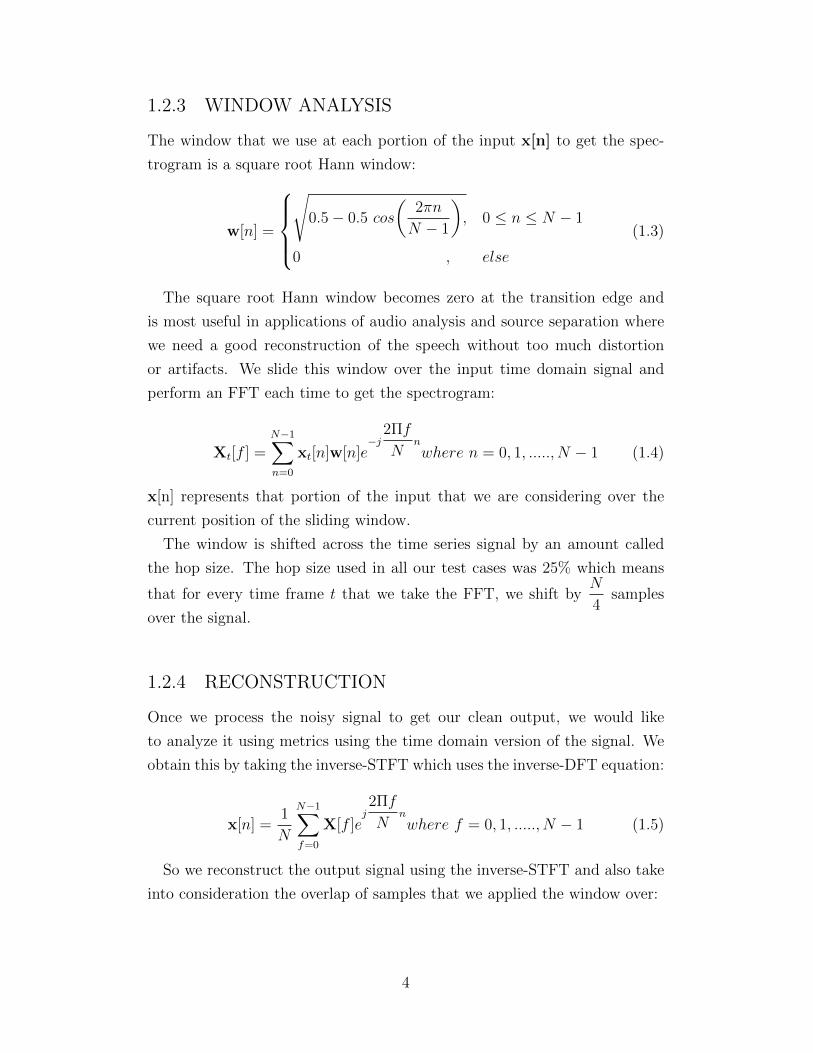
1.2.3 WINDOW ANALYSIS

The window that we use at each portion of the input x[n] to get the spec-

trogram is a square root Hann window:

w[n] =

√

0.5− 0.5 cos

(2πn

N − 1

), 0 ≤ n ≤ N − 1

0 , else

(1.3)

The square root Hann window becomes zero at the transition edge and

is most useful in applications of audio analysis and source separation where

we need a good reconstruction of the speech without too much distortion

or artifacts. We slide this window over the input time domain signal and

perform an FFT each time to get the spectrogram:

Xt[f ] =N−1∑n=0

xt[n]w[n]e−j

2Πf

Nnwhere n = 0, 1, ....., N − 1 (1.4)

x[n] represents that portion of the input that we are considering over the

current position of the sliding window.

The window is shifted across the time series signal by an amount called

the hop size. The hop size used in all our test cases was 25% which means

that for every time frame t that we take the FFT, we shift byN

4samples

over the signal.

1.2.4 RECONSTRUCTION

Once we process the noisy signal to get our clean output, we would like

to analyze it using metrics using the time domain version of the signal. We

obtain this by taking the inverse-STFT which uses the inverse-DFT equation:

x[n] =1

N

N−1∑f=0

X[f ]ej2Πf

Nnwhere f = 0, 1, ....., N − 1 (1.5)

So we reconstruct the output signal using the inverse-STFT and also take

into consideration the overlap of samples that we applied the window over:

4

x[n] =T−1∑t=0

(F−1(Xt[f ])w[n]

)∗ δ(n− tN

4) (1.6)

where implies elementwise multiplication and ∗ is convolution. δ(n−tN4

) is

the Kronecker delta shifted by tN

4samples which accounts for the overlap of

samples taken while performing the FFT operation with the sliding window.

When we take the STFT of the signal, we get a complex valued spectrogram

as the result. But we do not take phase into account in any of the algorithms

we used as we deal mainly with extracting the spectral and temporal features

of the audio signal and build models based on that. So we save the phase of

the spectrogram:

P (X[f ]) =X[f ]

|X[f ]|(1.7)

where abs(X[f ]) is the absolute valued spectrogram where we just take into

account the magnitude of the complex values. Before we perform the inverse-

STFT in equation 1.6 we apply this saved phase to the processed clean signal:

X[f ] = X[f ] P (X[f ]) (1.8)

where X[f ] is the real-valued spectrogram of the clean speech output from

the algorithm.

1.3 TRAINING CASES

All results shown in this thesis were based mainly on three cases. These

cases are different from each other in terms of the training information and

its similarity to the test cases.

1.3.1 FULLY-SUPERVISED

First we consider the fully-supervised case, where we use random utterances

of a speaker in training and test on a sentence of the same speaker. Similarly,

we train on the same noise type as we use in the test signal. This way the

training process builds accurate speech and noise models that form a good

5

representation of the sources in the noisy test signal.

1.3.2 SEMI-SUPERVISED

Second is the semi-supervised case where we train on the speech of the same

speaker as in the test, but the noise training will be something random. So

the trained model contains a good representation of the speech but may not

have an accurate idea of what the noise might be.

1.3.3 UNSUPERVISED

Third is the unsupervised case where we build a model based on no prior

information of the test speaker’s speech or the noise in the background. This

makes it hard for the system to differentiate between speech and noise in

general. For that reason we use speech of some random speakers in training

so that we can teach the model what speech in general sounds like, not the

specific speaker. This way we can test on any speaker keeping the training

process fixed. The noise as in the previous case can be anything random for

training. The last unsupervised case is what we would like to build ideally

as it is a very good real-world case.

1.4 TEST CASES

We modeled two scenarios for all test cases. In one scenario, we do denoising

offline, which means that we get the signal as a whole and process all the

time frames together. In the other, a more real-world scenario, we do de-

noising of the speech online or in real-time. This case is applicable to speech

recognition systems where the speaker is constantly talking and system is

trying to transcribe in real-time. This is a more difficult case of denoising

especially in semi-supervised and unsupervised cases since we do not have all

the information about one or both sources in the test signal. So we cannot

build an accurate enough model for the unknown sources in real-time. We

elaborate measures taken to prevent this overfitting while training online for

each algorithm in the later sections. So the maximum number of frames that

can be processed at a time to maintain this real-time scenario depends on

6

the sampling rate and window hop-size as well. Ideally, a real-time speech

based system should be able to process signals at least every second.

1.5 DATASETS

The speech examples used for training speech models and generating test

signals were obtained from the TIMIT Database [5]. This database contains

speech of different speakers, specifically 10 sentences of each speaker. For

training purposes, we used a randomly chosen 9 of these sentences so that we

can test on the left out 10th utterance. This forms a case of cross-validation

testing where we split the dataset into training and test and assign the data

samples randomly each time. For unsupervised cases, we had a big training

set where we used all 10 utterances of say 10 or 20 speakers. This was still

reasonable because we tested on the sentences of speakers different from the

ones in training. There is very little overlap between the content of speech

in the different speakers’ dataset, so there is no bias involved in training the

unsupervised case.

Different noise types have been used to account for all the real-world noises

and results were shown as an average performance across all these noise types.

To simulate noisy environments in the background of speech, we used noise

datasets from [7]. These contain a mixture of stationary, semi-stationary

and non-stationary noise signals. Stationary noise is the easiest to source-

separate as there is a specific pattern in its structure that can be easily learned

as features looking at the spectrogram. Semi-stationary and non-stationary

noise types are more difficult to separate as it is hard to learn features based

on their training signal. These noise types are more random and can have

different spectral and temporal structure in their spectrogram. Having just

a fraction of this type of noise in training might not accurately represent

what is present in the test signal. The test signal could be having the same

noise type as the trained features, but the extract and content specifically

might be slightly different as there are different variations to this noise type.

But in case of stationary noise, the features learned in training are adequate

to represent the noise in the test signal due to uniformity in spectral and

temporal patterns.

7

1.6 IDEAL SOURCE SEPARATION

Figure 1.3 shows an input noisy mixture, which is the spectrogram on the left,

to the model trained by a source separation algorithm. Ideally we should get

the clean spectrogram out as shown in the center figure which corresponds

to the exact same speech as in the noisy mixture without any distortions or

alterations. In the real-world case, this is probably not possible as there will

be some interference from the other sources and some artifacts introduced in

the speech. This is because we cannot achieve near perfect training models in

the real-world. In this thesis, we indicate the performances of each algorithm

and show how one is better than the other.

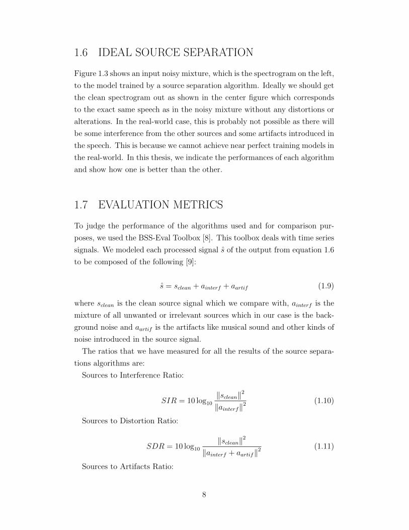
1.7 EVALUATION METRICS

To judge the performance of the algorithms used and for comparison pur-

poses, we used the BSS-Eval Toolbox [8]. This toolbox deals with time series

signals. We modeled each processed signal s of the output from equation 1.6

to be composed of the following [9]:

s = sclean + ainterf + aartif (1.9)

where sclean is the clean source signal which we compare with, ainterf is the

mixture of all unwanted or irrelevant sources which in our case is the back-

ground noise and aartif is the artifacts like musical sound and other kinds of

noise introduced in the source signal.

The ratios that we have measured for all the results of the source separa-

tions algorithms are:

Sources to Interference Ratio:

SIR = 10 log10

‖sclean‖2

‖ainterf‖2(1.10)

Sources to Distortion Ratio:

SDR = 10 log10

‖sclean‖2

‖ainterf + aartif‖2(1.11)

Sources to Artifacts Ratio:

8

Figure 1.3: The spectrogram on the left is one of a noisy signal which is amixture of a 2 s speech signal and some casino background noise [7]. Thespectrogram in the middle is the ideal clean speech source in the mixtureand the one on the right is the noise that was mixed with this speech signal.

SAR = 10 log10

‖sclean + ainterf‖2

‖aartif‖2(1.12)

The SIR is a good measure to evaluate the source separation quality. It

gives us an idea of how much the source we are talking about has been

separated from all the other sources. The SDR and SAR give us an idea

of how much the algorithm has distorted the speech signal and varied it

by introducing artifacts. There is always a tradeoff between the SIR and

SDR/SAR figures, as when source separation quality is high, we have a more

distorted or altered speech signal. When we have a better quality output

speech signal, we can probably still hear some parts of the other sources

mixed in with the source in context.

1.8 TOOLS

The algorithm for the NMF based approach was implemented mainly in

MATLAB and used a CPU with a 2.2 GHz Intel quad-core i-7 processor.

Initially the fully-connected neural networks were implemented in MATLAB,

but we later moved to using third-party tools for accuracy and handling

bigger datasets better. We mainly used two tools for making neural network

models: Caffe [10] and Keras [11].

Caffe is a vision-based deep learning software made at the Berkeley Vision

and Learning Center (BVLC) and is focused mainly on solving computer

9

vision problems. We used this software to make models for audio and solve

regression problems, which in our case were speech denoising. We generated

datasets and did the initial setup in MATLAB, then fed the data and param-

eters to be run on the Caffe framework. We used a Tesla K20 GPU during

the training process as neural network training requires much computation.

Keras is a Theano-based deep learning library. It can be used only on

Python and requires the use of Theano software [12], [13] as well. Theano

is a Python library that is useful for multi-dimensional array processing and

has been widely used for deep learning research. Keras is a tool that is built

on a layer above Theano and has its own functions that implement any neural

network architecture necessary without having to build upon the algorithm

from the ground up as in Theano. We used a Tesla K40 GPU to train the

neural networks designed on this software.

1.9 CONTRIBUTIONS

In previous work on source separation problems, we either assume training

information of the speaker or the noise type in the background. Most of these

models are offline based and need the whole signal in order to perform the

denoising.

In this thesis we have used two methods for denoising: nonnegative matrix

factorization and neural networks. We have shown the performance of the

unsupervised case where we do not have any prior training information of the

speaker or noise type in the signal for both these methods. The degradation

in performance for this case is not very drastic compared to that of the fully-

supervised case. We have also proposed how to perform these methods in

real-time where the denoising can be done frame by frame or for a group

of frames together. Even this case had performance that was not too much

worse than the offline method. Hence we have developed two robust models

that can denoise any noisy signal, regardless of the speaker and the noise type,

and in real-time. Also we have used various noise examples that are different

from each other and both genders of speakers to generate the results. This

shows that our algorithms can be used in a real-time voice recognition device

in order to perform the prior denoising to improve the speech recognition

accuracy.

10

CHAPTER 2

NONNEGATIVE MATRIXFACTORIZATION

2.1 NMF INTRODUCTION

The first method we used to solve this problem of speech denoising is one

using nonnegative matrix factorization (NMF). It assumes the input data

to be nonnegative and imposes nonnegativity on the features it produces as

well. NMF has been used to solve source separation problems in applications

of music [14] and multi-speaker separation [15].

In this section, we introduce the theory behind the NMF algorithm in

general and then propose a modification of this in order to develop a real-

world system that is robust enough to denoise any signal without any prior

information of the test speaker or the noise in the test signal. Additionally

we show that the denoising performance of this method is close enough to

methods that have these additional requirements, thereby making it a viable

alternative. In addition to demonstrating the performance of this approach,

we also illustrate some of the tradeoffs that one might find in the parameters

involved and how they influence performance.

2.1.1 DEFINITION

It is a method in which we can decompose an input matrix into two con-

stituent matrices. Hence given an input matrix V, we can decompose it

into:

V ≈W ·H (2.1)

This method imposes a constraint of nonnegativity on all the matrices.

Given a matrix V with all nonnegative values, this decomposes it into two

nonnegative matrices W and H. NMF is a method of analyzing or decom-

11

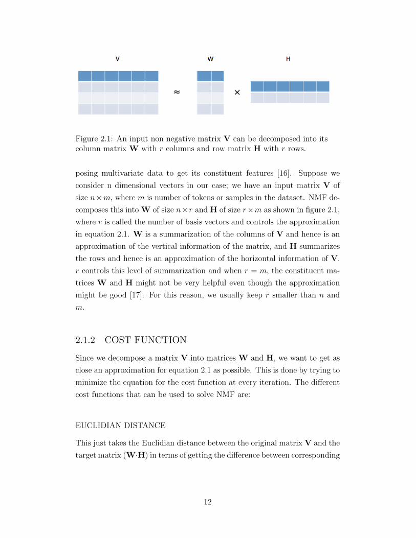
Figure 2.1: An input non negative matrix V can be decomposed into itscolumn matrix W with r columns and row matrix H with r rows.

posing multivariate data to get its constituent features [16]. Suppose we

consider n dimensional vectors in our case; we have an input matrix V of

size n×m, where m is number of tokens or samples in the dataset. NMF de-

composes this into W of size n×r and H of size r×m as shown in figure 2.1,

where r is called the number of basis vectors and controls the approximation

in equation 2.1. W is a summarization of the columns of V and hence is an

approximation of the vertical information of the matrix, and H summarizes

the rows and hence is an approximation of the horizontal information of V.

r controls this level of summarization and when r = m, the constituent ma-

trices W and H might not be very helpful even though the approximation

might be good [17]. For this reason, we usually keep r smaller than n and

m.

2.1.2 COST FUNCTION

Since we decompose a matrix V into matrices W and H, we want to get as

close an approximation for equation 2.1 as possible. This is done by trying to

minimize the equation for the cost function at every iteration. The different

cost functions that can be used to solve NMF are:

EUCLIDIAN DISTANCE

This just takes the Euclidian distance between the original matrix V and the

target matrix (W·H) in terms of getting the difference between corresponding

12

elements in each matrix.

C = ‖V−WH‖2 =∑ij

(Vij − (WH)ij)2 (2.2)

where i, j are the row and column indices respectively of each matrix where

i ∈ [1, n] and j ∈ [1,m].

KULLBACK-LIEBLER DIVERGENCE

This is more a non-symmetric measure of how much two matrices differ from

each other. It measures the relative entropy between the two matrices. In

the case of NMF, the cost function becomes the divergence equation:

C = D(V‖WH) =∑ij

(Vij log

Vij

(WH)ij−Vij + (WH)ij

)(2.3)

where i, j are the row and column indices respectively of each matrix where

i ∈ [1, n] and j ∈ [1,m].

IKATURA-SAITO DIVERGENCE

Another function which has commonly been used for speech and audio is the

Ikatura-Saito (IS) divergence function [18]:

C = DIS(V‖WH) =∑ij

( Vij

(WH)ij− log

Vij

(WH)ij− 1)

(2.4)

2.1.3 SIMILARITY TO PCA

Principal component analysis (PCA) is a method in which we get features

from a data matrix similar to the matrix V that we have been talking about

in NMF. PCA gives us eigenvectors of this matrix and can be used to project

into a different feature space where the dimensionality of the vectors, which

was previously n, changes.

H = A ·V (2.5)

13

where A is the feature matrix containing the eigenvectors of the input matrix

V and H is the new feature space with m vectors of different dimensions.

As can be seen, this is similar to the NMF equation if we take the Moore-

Penrose inverse of the W matrix which is denoted in equation 2.6 by W+.

H = W+ V (2.6)

Since PCA models the feature matrix by stacking the eigenvectors of the

input together, it imposes the orthogonality constraint. PCA hence tries to

solve the same cost function with the orthogonality constraint [17].

2.1.4 KL-NMF ALGORITHM

This uses the Kullback-Liebler (KL) Divergence equation for the cost function

and hence we take the derivative of equation 2.3 with respect to W and H

to find the local minima of this function. We use gradient descent in order

to update the W and H at every iteration to get as close an approximation

as possible.

GRADIENT DESCENT

The gradient descent equation is such that we move on the steep part of the

convex curve and reach the point of local minimum:

xl+1 ← xl − η∇f(xl) (2.7)

where xl+1 is the variable at the next iteration and the current value of the

variable xl is being used to update the value at every iteration. Matrices W

and H are updated this way. η is the step-size with which we move on the

curve and ∇ implies gradient with respect to x.

UPDATE EQUATIONS

(W,H) = W,H≥0D(V‖W H) (2.8)

W←W

(V

W·H ·H>

1 ·H>

)(2.9)

14

H← H

(W> · V

W·H

W> · 1

)(2.10)

where implies element-wise multiplication and the fraction implies element-

wise division. These updates are repeated until we reach convergence which

will be a local minimum of the divergence function. This point is not guar-

anteed to be a global minimum since we have a non-convex function, but in

practice it often finds a usable solution.

2.1.5 APPLICATION IN MUSIC AND AUDIO

NMF has been used widely in audio applications to solve problems of single

and multi-channel source separation problems [19]. The separation could

be sources of different musical instruments, singing voices, speech of various

speakers or speech denoising as in our case.

Since NMF decomposes the input nonnegative matrix V into its column

summarization W and row summarization H, we can use an absolute valued

spectrogram of the mixture or source as the input to the NMF algorithm.

W will give us an approximation of the spectral information and H will give

us an approximation of the temporal information or time activations. Figure

2.3 shows a spectrogram of four piano notes played together decomposed into

its constituent spectral and time activation matrices. We took r = 4 as we

have four notes in the excerpt. As explained before, W shows the frequency

or spectral information of each of the notes individually as each column or

basis vector. Similarly H shows the respective time activation of each note

in the respective row [17]. If we want to separate the sound of a single note,

we can do:

Vn = Wn ·Hn (2.11)

where n corresponds to the basis vector of the specific note.

The basis vector representation is a little more complex for speech and

noise. The speech source will correspond to a collection of these basis vectors

and a single basis vector might not be able to explain much about either

source. So we allocate a certain number of basis vectors for speech and noise

separately and source-separate using only those basis vectors. So n from

15

Figure 2.2: This is a simple spectrogram from that shows activity of mainlytwo frequencies [17].

Figure 2.3: This is the NMF decomposition of the spectrogram in figure 2.2with r = 2 where the columns of the W matrix show the two frequenciesand the rows of the H matrix show the respective time activations [17].

16

equation 2.11 will correspond to a group of basis vectors allocated for the

desired source.

2.2 MODIFIED NMF ALGORITHM

Nonnegative matrix factorization (NMF) and probabilistic latent component

analysis (PLCA) have been used for source separation tasks in a variety

of situations [19], [20], [15], with a very common use being that of speech

denoising [21]. Although these methods can perform well, they often neces-

sitate that the speaker in the provided mixtures is known a priori or even

the noise type and that an appropriate model for that source has already

been constructed. Furthermore, many of these approaches are offline which

when combined with the previous requirement makes for a system that is

not amenable to real-world use. Recently we have seen the introduction of

systems that do not require a priori knowledge of the speaker in the mixture

[22] and models that can operate in an online manner [7, 23, 18]. In this

research we propose an algorithm that combines these features to create a

system that is well suited for real-world deployment since it does not require

advance knowledge of the speaker or the noise in a mixture; it can operate

in an online manner which facilitates a real-time implementation, and it is

efficient enough to run in real-time without excessive hardware requirements.

2.2.1 FULLY-SUPERVISED

This is the case where we have prior information of the test speaker’s speech

and of the noise type in the background of the test signal as well. In the case

of NMF, this is obtained by performing the KL-NMF algorithm using some

training signals. This equation for NMF is roughly equivalent to PLCA

[24] which has been used for denoising in more real-world cases [7], [23].

When we talk about having prior information of the speaker, we refer to

the model having some knowledge of what the source might sound like. The

spectral features of the source which are given by W can be used in our

case. We call this is a speech or noise dictionary based on the source. We

use KL-NMF for training and testing alike as we want to reach the same

local minimum. Hence in the training process, we learn WS, which is the

17

speech dictionary, and WN , which is the noise dictionary, and discard the

respective time activations HS and HN , which are irrelevant in our case due

to the speaker having to say different things in training and test. The test

process tried to solve the equation:

H = W,H≥0D (V||[WS,WN ] ·H) (2.12)

where W = [WS,WN ] is the fixed dictionary from training and hence we

do not update this during the test process. The activations H can be then

represented as

[HS

HN

], that is in parts that contain the activations HS of

the speech bases WS and the activations HN of the noise bases WN . The

clean speech magnitude spectrogram can then be recovered as VS = WS ·HS.

Using the phase of the original sound we can transform VS back to the time

domain and obtain a speech waveform. Instead of the reconstruction shown

above, we can also use alternative approximations:

VS = VWS ·HS

W ·H(2.13)

2.2.2 SEMI-SUPERVISED

In this research we also use KL-NMF in the context of the semi-supervised

denoising method [7]. We do so because we want to deploy this model in

situations where the noise in the recordings is not known and needs to be

automatically estimated. In this case, we can use KL-NMF to build a speaker

dictionary WS using as input the magnitude spectrogram VS of a speech

training example. Once this speaker dictionary is obtained we can fix it and

decompose a mixture containing the voice of that speaker plus noise. Thus,

for a mixture magnitude spectrogram V, we estimate the activations H and

a noise dictionary WN by solving the problem:

(WN ,H) = W,H≥0D (V||[WS,WN ] ·H) (2.14)

Estimating WS and H can be easily done by a simple modification of the

update equations 2.9 and 2.10.

18

2.2.3 UNIVERSAL SPEECH MODEL

We now consider the unsupervised case where we have no training informa-

tion of the particular speaker or noise type in test. Since we are using a

model of speech with no prior information of the speaker, we can apply what

is a called a universal speech model (USM) obtained by training on multi-

ple male and female speakers. By allocating multiple basis vectors for each

speaker and training on M speakers using KL-NMF, we obtain a USM by

concatenating each speaker’s dictionary Wi to a larger USM dictionary:

WUSM = [W1,W2, · · · ,WM ] (2.15)

Our speech dictionary now contains information from M different speakers

with their basis vectors grouped together in blocks.

2.2.4 BLOCK SPARSITY

As shown in [22], using all this information to model the time activations of

one speaker might cause overfitting leading to a degraded speech output. To

alleviate this we can impose a sparsity constraint on the activation matrix in

order to use information of the speaker closest to the one in the signal. More

specifically, we use block sparsity where the sparsity constraint is imposed

on each block, i.e., on the set of basis vectors representing each speaker.

This forces the fitting process to predominantly choose the basis vectors of

a speaker who is most similar sounding to the one in the input signal. This

is enforced through the following modified cost function:

(W,H) =W,H≥0 D(V||W ·H) + λΩ(HS) (2.16)

where the Ω is the penalty imposed to induce sparsity in the speech activation

matrix HS [22]. The parameter λ can be adjusted to control how much energy

we draw from one speaker. A large λ uses only one speaker’s basis vectors.

The separation from noise tends to be good but it introduces a lot of artifacts

into the speech. A smaller λ allows the fitting to use all the speakers’ basis

vectors. This induces fewer artifacts but the noise is not removed as well

since it can be modelled through various bases from other speakers. Tuning

the parameter λ allows us to optimize this trade-off and can be appropriately

19

adjusted. This is shown in figure 2.4. The three figures depict how the tuning

of λ affects the source separation quality. In [22] and [18] we see the use of

a log /l1 penalty for block sparsity as convergence can be achieved using

multiplicative updates which fits well with our model. The sparsity penalty

is defined as:

log /l1 =M∑i=1

log(ε+ ||Hi||1) (2.17)

where Hi is the subset of H that corresponds to speaker i.

ADDITIONAL WEIGHT

We make one more addition to the USM model in order to achieve better

speech separation from the noise. At each iteration of training we add a

constant nonnegative value w to all the elements of H that correspond to the

noise bases. This allows us to specify how much energy from the mixture we

want to allocate to the noise model or the speech model. Like the sparsity

constraint, this also introduces artifacts in the speech since it might allocate

some of the speech energy to the noise, but it dramatically improves the

separation when properly tuned.

2.2.5 BKL-NMF ALGORITHM

Since we model the NMF such that the basis vectors are divided into blocks

based on many speakers or a single speaker used in the training process,

we refer to this modified approach as Block Kullback-Liebler nonnegative

matrix factorization (BKL-NMF). We use the BKL-NMF algorithm for both

training and test purposes. The training algorithm is shown in algorithm 1

as pseudocode. This algorithm is performed for the M speakers we use in

training. In supervised and semi-supervised cases, we have M = 1 as we

train on the same speaker’s speech. In the unsupervised case, M is greater

than 1, generally in the order of 10 to 20. Our input is the spectrogram of

the training excerpt of the speaker in context. We randomly initialize speech

dictionary W and speech activations H since we do not have any knowledge

of them in the beginning. We then perform equations 2.9 and 2.10 until we

reach an optimum or a point of local minima. In the end, we concatenate

20

λ = 0 λ = 50 λ = 200

Figure 2.4: This figure shows the sparsity imposed in the HS matrix. Thisis the time activations matrix when we use a universal speech model fortraining with multiple speakers. The color scale is such that the darker theregion in the matrix, the more sparse the matrix. There are three cases: 1.On the extreme left, λ = 0. There is no sparsity imposed and hence everyspeaker’s basis vectors have the same energy. 2. The middle figure withλ = 50, where the energy is drawn from the basis vectors of a group ofspeakers. This case balances the source separation and artifacts tradeoff. 3.The rightmost figure with lambda = 200 picks up the basis vectors of onlyone speaker. In this test case, we used a female speaker and the USMcontains 10 male speakers followed by 10 female speakers in training. Hencethe algorithm picked up a female speaker’s dictionary. This is the case ofhigh λ which leads to high source separation but more artifacts in thespeech.

21

Algorithm 1 BKL-NMF Training

for i = 1 : M doinputs Xi

initialize random Wi, Hi

repeatRi = Xi

Wi·Hi

Wi = Wi (Ri ·H>i

)renormalize the columns of Wi to 1

Hi = Hi (W>

i ·Ri

)renormalize the rows of Hi to 1

until convergence

end for

WUSM = [W1,W2, · · · ,WM ]

these training matrices in unsupervised cases to obtain the universal speech

model WUSM .

The test algorithm is slightly different as we keep the speech dictionary

fixed and learn the activations and also the noise dictionary in case of the

semi-supervised and unsupervised. This is shown in algorithm 2. We have

inputs X, which is the input noisy test spectrogram to be denoised and

WUSM , which is the universal speech dictionary or simple single speaker

training dictionary obtained from algorithm 1. We initialize random positive

speech and time activation matrices H and the noise dictionary WN in case

of semi-supervised and unsupervised cases. So we perform the update for H

similar to training, but in the case of the dictionary, only the noise dictionary

is updated for the related cases. In the case of unsupervised alone, we impose

the log/l1 sparsity constraint with a chosen value of λ on the H matrix. We

do this individually M times on each block of H with the basis vectors

allocated for each speaker included in the USM. We then add the weight

to the noise block of H to improve the source separation performance. The

noise dictionary WN is then updated based on the new values of H.

22

Algorithm 2 BKL-NMF Test

inputs X, WUSM

if supervised theninput WN from training

elseinitialize random WN

end if

initialize random H =

[HS

HN

]repeat

W = [WUSM ,WN ]R = X

W·HH = H (W> ·R)if unsupervised then

for i = 1 : M doHSi ← HSi

11+ λ

ε+||HSi ||1

end forend ifHN = HN + wif semi-supervised or unsupervised then

A = W (R ·H>)WN = AN

renormalize columns of WN to sum to 1end if

until convergence

23

Finally we reconstruct the clean speech spectrogram VS using:

VS = WUSM ·HS (2.18)

In the unsupervised case, the sparsity imposed on HS ensures that only a

few basis vectors corresponding to a specific speaker or selection of speakers

are activated when performing this reconstruction.

2.2.6 ONLINE METHOD

In order to perform online or real-time denoising we need to process input

magnitude spectrum frames as they appear. Therefore, once we train a USM

or a single speaker’s speech dictionary we can apply it on every input frame or

a group of frames of the mixture spectrogram individually. In semi-supervised

and unsupervised cases, we need to appropriately update a noise model WN ,

thus estimating the noise dictionary and its respective activations.

Updating the noise dictionary in the two cases might not be as straight-

forward as in the offline method. This is because we are trying to fit some

information about noise using just a single spectrogram frame. We need to

allocate some number of basis vectors to model the noise dictionary accu-

rately, but modeling this based on a single frame will lead to overfitting. So

we can model the noise dictionary WN based on not only the current frame

but some previous frames in the past. This way we are fitting the dictionary

based noise information from many samples which will give us a much more

accurate representation of the noise source. Also, instead of creating a new

noise dictionary while denoising each frame, we can update the WN of the

previous frame using some weights:

A = (1− µ)(W (RG ·H>G)) + µ(W (RB ·H>B)) (2.19)

We denote the time indices of the input frames currently being denoised

by G. In addition to the current input frames VG, we maintain a running

buffer B containing the b frames directly preceding VG. The variable HG

contains the basis activations for the current frames and HB contains the

activations for the frames maintained in the buffer. Operating on this set

prevents potential overfitting as we are estimating the basis vectors of the

24

noise dictionary using multiple time frames and not just one or a small num-

ber of frames from the input [23]. µ here is the weight we decide to impose

on the information from our buffer B and is between the values of 0 and 1.

Hence we apply a weight of 1−µ on the current frame and its activation HG.

Algorithm 3 describes the BKL-NMF algorithm taking the buffer B into

consideration. HG is split into the activations that relate to the speakers

HGS and the noise HGN . The speaker activations are furthermore split into

sets that correspond to each speaker HGSi in the unsupervised case. The

activations for the previous b frames are saved in matrix HB after being cal-

culated in preceding steps. This is the same process described in Algorithm

2, but at every step instead of using all frames of the input noisy signal to-

gether, we only denoise the current g frames and use an additional b frames

from the running buffer. We impose the weights µ and 1 − µ as described

above to model the noise dictionary based on current frames and the previous

frames in the buffer. At the end of this process we will have estimated an

updated noise model and an estimate of the speaker’s magnitude spectrum

as: VSG = WUSM ·HSG.

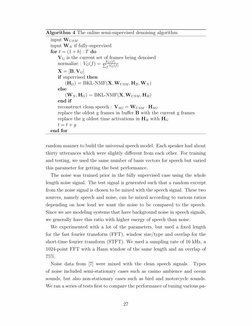
The main online BKL-NMF algorithm is represented in Algorithm 4. This

does the denoising of any noisy speech signal in real-time and can be used for

any of the training cases described earlier. Once we get the dictionary from

training, we can denoise frame by frame or a bunch of frames together based

on how fast we want our model to work. We skip denoising the first b frames

of the signal since we need to maintain a buffer of that size to model the

activations and the noise dictionary as well in some cases. We normalize the

current spectrogram VG containing the frames being denoised to maintain a

probability based model like in [7]. We then input the pretrained dictionaries,

frames containing VG and those in the buffer B and the time activations HB

of the frames in B to the BKL-NMF algorithm described in Algorithm 3. This

is used as a subroutine for every set of frames to obtain the time activations

HG and noise dictionary WN in the semi-supervised and unsupervised cases.

This is the same as Algorithm 2 but with the buffer of previous frames and

their activations taken into account as well. After this, we reconstruct the

clean signal of those frames VSG using reconstruction WUSM ·HSG. At every

iteration of the set of frames we denoise, we update the buffer B by replacing

the oldest g frames with the current frames that we denoised. This is so that

for the next g frames we denoise, we are modeling parameters based on a

25

Algorithm 3 BKL-NMF

inputs X, WUSM , HB

if supervised theninput WN from training

elseinitialize random WN

end if

initialize random HG =

[HGS

HGN

]repeat

W = [WUSM ,WN ]R = X

W·H = [RB,RG]

HG = HG (W> ·RG)if unsupervised then

for i = 1 : M doHGSi ← HGSi

11+ λ

ε+||HGSi ||1

end forend ifHN = HN + wif unsupervised or semi-supervised then

A = (1− µ)(W (RG ·H>G)) + µ(W (RB ·H>B))WN = AN

renormalize columns of WN to sum to 1end if

until convergence

buffer with the last b frames. Similarly we update HG as well to prevent the

model from overfitting.

2.3 EXPERIMENTS AND RESULTS

The model was tested as a real-time speech denoising tool. The TIMIT

database was used for training the speech dictionary. This database has 10

spoken sentences for each speaker and has a large collection of male and

female speakers and accents based on regions in the United States.

For the fully supervised and semi-supervised cases, we used a random one

of these sentences in the test signal and trained on the remaining 9 sentences.

In the unsupervised case, we picked ten male and ten female speakers in a

26

Algorithm 4 The online semi-supervised denoising algorithm

input WUSM

input WN if fully-supervisedfor t = (1 + b) : T do

VG is the current set of frames being denoisednormalize : VG(f) = VG(f)∑

f VG(f)

X = [B,VG]if supervised then

(HG) = BKL-NMF(X,WUSM ,HB,WN)else

(WN ,HG) = BKL-NMF(X,WUSM ,HB)end ifreconstruct clean speech : VSG = WUSM ·HSG

replace the oldest g frames in buffer B with the current g framesreplace the g oldest time activations in HB with HG

t = t+ gend for

random manner to build the universal speech model. Each speaker had about

thirty utterances which were slightly different from each other. For training

and testing, we used the same number of basis vectors for speech but varied

this parameter for getting the best performance.

The noise was trained prior in the fully supervised case using the whole

length noise signal. The test signal is generated such that a random excerpt

from the noise signal is chosen to be mixed with the speech signal. These two

sources, namely speech and noise, can be mixed according to various ratios

depending on how loud we want the noise to be compared to the speech.

Since we are modeling systems that have background noise in speech signals,

we generally have this ratio with higher energy of speech than noise.

We experimented with a lot of the parameters, but used a fixed length

for the fast fourier transform (FFT), window size/type and overlap for the

short-time fourier transform (STFT). We used a sampling rate of 16 kHz, a

1024-point FFT with a Hann window of the same length and an overlap of

75%.

Noise data from [7] were mixed with the clean speech signals. Types

of noise included semi-stationary cases such as casino ambience and ocean

sounds, but also non-stationary cases such as bird and motorcycle sounds.

We ran a series of tests first to compare the performance of tuning various pa-

27

rameters in the algorithm. We then tested the algorithm on the three cases

of having different training information. It is important to determine the

degradation in performance as you have less training. Also the online case

models parameters based only on a few frames, so we ran tests to compare

how well this performs compared to the offline method.

The parameters that were varied to test the performance of the algorithm

under different noise conditions, genders and noise levels are: λ, w, µ, number

of speech and noise basis vectors. The results for these are shown in figures

2.5, 2.6 and 2.7. As can be seen, varying these parameters affects the values

of the SIR, SAR and SDR ratios. The source separation quality measured

by SIR and artifacts ratios measured by SAR are inversely related and this

proves the existence of the trade-off between these two. After various tests,

we tried to balance the trade-off between the SIR and SAR [23]. We decided

to use λ = 10, w = 1, µ = 1/3, G = 40 frames at a time, size of buffer

B = 60, 40 speech basis vectors for each speaker for training and testing and

20 noise basis vectors in the offline case, and 5 noise basis vectors for every

iteration in the real-time case. The SIR and SAR values of the clean output

speech signals for all the cases were obtained using the BSS-eval toolbox [8].

The results of these experiments, averaged over all the speakers and noises

are shown in figures 2.8 and 2.9. Figure 2.8 compares the performances

of the algorithm in the fully-supervised, semi-supervised and unsupervised

training cases. The fully-supervised case performs the best because of having

a dictionary of the test speaker in advance and also having an idea of the noise

type in the background. The semi-supervised case does not have training

information of the noise in advance and hence uses a randomly declared

positive matrix as the noise dictionary. The unsupervised case used some

random speech from 10 male speakers and 10 female speakers as the universal

speech model and a random noise dictionary. These two cases, even though

having little or no prior information of the test signal, perform well and are

not significantly inferior to the fully-supervised case. There is only a 1-2 dB

dip from one case to another in the different ratios.

Figure 2.9 compares the performance of the online and offline algorithms

in the case of unsupervised training. The online algorithm processes the

signal frame by frame or with a bunch of frames put together. This leads to

problems of overfitting the noise dictionary. The online algorithm is almost

as good as the offline one. There is only a 2-3 dB dip in SIR and 1-2 dB

28

λ0 10 20 30 40 50 60 70 80

dB

-5

0

5

10

15

20

SIR

SAR

w0 0.5 1 1.5 2 2.5 3

dB

6

8

10

12

14

16

18

SIR

SAR

Figure 2.5: The figure on the left shows the performance of denoising of5dB mixture for different λ values. Increasing λ makes use of dictionaryelements from fewer speakers from the USM model and improves theoutput SIR at the expense of a reduced SAR. The figure on the right showsthe performance of the algorithm for different w values. By boosting w, weallow the noise dictionary to explain more of the input mixture, thusremoving more noise and improving the final SIR, but degrading the speechsignal and reducing the SAR.

decrease in SDR/SAR.

2.4 CONCLUSION

NMF has been used in many previous cases for source separation. It has

proved to be a good tool for speech denoising as well. In our case, we have

developed a model where we do not need any prior information of the speaker

or noise. It is a real-time speech denoising tool that does the denoising when

given just a general idea of speech.

The disadvantage with the unsupervised case is that it picks up any speech

from the background as well. This is because of the universal speech model

with sparsity that tries to activate any speech in the signal. The supervised

and semi-supervised cases do a better job in this scenario due to their speech

dictionaries containing spectral information of the particular speaker. This

approach of unsupervised real-time speech denoising does come at a cost of

lower source separation performance and degraded speech quality. But as

shown by figure 2.8, the degradation is not too much and the performance

of the unsupervised is quite comparable to the fully supervised case. In

the real-world when trying to use a speech denoising tool, we cannot expect

to have training of the noise type because of the randomness of what is

29

µ

0 0.1 0.2 0.3 0.4 0.5 0.6 0.7 0.8 0.9 1

dB

8

8.5

9

9.5

10

10.5

11

11.5

12

12.5

SIR

SAR

frame groups (G)0 10 20 30 40 50 60

dB

0

2

4

6

8

10

12

14

16

SIRSAR

Figure 2.6: The figure on the left shows the performance of the algorithmfor different µ values. A small µ allows us to adapt to the noise sourcefaster, producing a higher SIR, but results in degrading the speech signal inthe process and reducing the SAR. The figure on the right shows theperformance of the algorithm for different g values. By fitting the data tomore frames we get more averaging, which decreases the SIR but improvesthe SAR.

called noise. It could be from a wide range of sources like vehicles, musical

instruments, channel distortion, commotion of people like footsteps, etc. A

robust model would work for any speaker speaking to the system. In case of

a voice recognition system, we want the denoising to be done in real-time and

independent of the speaker. The model that we have developed does a good

job of achieving this goal in terms of information required and performance.

The main contributions from this chapter are that we have developed an

NMF model that uses a general speech dictionary USM and a random positive

noise dictionary to perform the denoising of a signal. Through algorithm 4

we have shown that this is an online model and performs well with some

artifacts. We have used both male and female speakers and different noise

types in the test cases to generate the shown results. This proves that our

unsupervised NMF algorithm is very robust and performs independently of

the type of speaker, speech and noise in the background.

30

Figure 2.7: The change in SIR and SAR measures plotted against thechange in basis vectors allocated for speech. The trend is similar in thatthere is an inverse relation between the two. Using lesser basis vectors forspeech does good noise separation but cannot model the speech well due tounder-fitting. Similarly, using a lot of basis vectors models the speech wellby learning more information, but this comes at the cost of sourceseparation.

31

SDR SIR SAR

dB

0

5

10

15

20

25Comparison of training cases

fully-supervisedsemi-supervisedunsupervised

Figure 2.8: The figure compares the performance of the three differenttraining cases: fully-supervised, semi-supervised, unsupervised. Thedenoising was done offline. As expected, the fully-supervised case performsthe best, followed by semi-supervised and then unsupervised. But they arequite comparable as the degradation is not too great.

SDR SIR SAR

dB

0

5

10

15Offline vs Real-Time Denoising

offline

online

Figure 2.9: This figure compares the performance of the algorithm offlineand in real-time with unsupervised training. The real-time case eventhough modeling the noise dictionary frame-by frame, has a comparableperformance to the offline version.

32

CHAPTER 3

NEURAL NETWORKS

3.1 NEURAL NETWORK INTRODUCTION

This chapter shows the use of fully-connected neural networks (FNN) for

speech denoising. Neural networks are being used recently in a wide range

of applications mainly for classification tasks or source separation problems

[25], [26]. We first introduce the theory behind neural network algorithms

and why they are a viable method to try to solve various problems. We then

explain the architecture used for our specific neural network and show results

to prove that the chosen parameters and options were most optimal.

The experiments in this section go over the three cases of training: fully-

supervised, semi-supervised and unsupervised. We try to model a system

where we do not need any training information of the speaker in test or of the

noise in the background. We show how this model, because of the additional

complexity and approach, performs better than the NMF algorithm explained

in the previous chapter. We also talk about how this algorithm can be

modeled in real-time.

3.2 THEORY

This section goes over the theory behind the formation of a neural network.

We start with classification for linear cases, how more complex non-linear

data is handled, and then to neural networks and how they are used for

regression.

33

3.2.1 LINEAR CLASSIFIER

The linear classifier creates a hyperplane across data points in order to clas-

sify them into labels. This is good for classifying multi-dimensional data as

it becomes more difficult to train Gaussians due to the requirement of a lot

of samples. The naive Bayes classifier assumes independence across dimen-

sions which might not be ideal in all cases [27]. A linear classifier creates a

boundary which is hyperdimensional and is relatively easy to train.

yn = w> · xn, n = 0...N − 1 samples (3.1)

where w is the weight matrix or the features learned to perform this clas-

sification and x is the data being classified. x is multi-dimensional with D

dimensions and N samples:

xn = [x1n,x

2n, · · · ,xDn ]T , n = 0...N − 1 (3.2)

w = [w1, w2, · · · , wD]T (3.3)

w is a feature matrix that transforms the input x into a new space. In this

case, w is only a vector since we just get a binary label. This is a case of

binary classification where we are trying to classify between two classes ω1

or ω2.

y = w> · xn > 0, choose ω1

y = w> · xn < 0, choose ω2

(3.4)

Figure 3.1a is a good representation of a binary linear classifier.

Multiclass classification is also possible where a w is learned between ev-

ery two classes. Hence we have different permutations of feature matrix w

between each pair of classes.

3.2.2 TRAINING USING GRADIENT DESCENT

In the training step, we need to fit a classifier such that there is zero error

in the labels we assign each sample. We need to choose an error function

such that we get a good estimate of the number of wrong labels. We use the

Euclidian distance equation to find error:

34

(a) Binary classified data separated bylinear classifier [28]

(b) The XOR case exemplifyingnon-linear data. This needs a differentclassifier, one with two decision lines [28]

Figure 3.1: The two figures above show examples of classification of linearand non-linear data.

e =N−1∑n=0

(yn − tn)2 (3.5)

We start with some random value of the weight matrix w and use gradient

descent to update it at every iteration so that we reach some point of local

minimum. This is done by:

wi+1 = wi − η ∂e∂w

(3.6)

where i is the current iteration of the gradient descent. Figure 3.2 shows how

gradient descent finds an optimum by descending slopes of the error function.

This minimum achieved could be a point of local or global minimum. The

global minimum is the most optimal point and reduces the error function

most. But it really depends on the starting point, which in our case is

random. The initialization of w in our case determines whether we reach a

local or global optimum.

3.2.3 NONLINEAR CLASSIFIER

The data in figure 3.1a is linear and hence we can model a linear classifier

to separate the two classes. If we take the case where we have data like in

the XOR case, the data is non-linear and hence the classifier above will not

35

Figure 3.2: This shows the various points of local minimum and the globalminimum. It portrays how the gradient descent in equation 3.6 goes abouttrying to minimize the error and reach an optimum [28].

work. We need a classifier like the one shown in figure 3.1b where we have

two decision lines [28].

This can be achieved by projecting the data into a different space so that it

becomes easily separable. So we use two layers to do this. As shown in figure

3.3, the first layer projects the data into a space that makes it much easier

to classify the data. The problem then becomes one of linear classification

and the second layer can do that easily. So this forms a two-layer neural net

as shown in figure 3.4 [28]. Similarly if this problem is still non-separable

after the first layer’s projection, we add one more layer such that the three-

layer network has two layers for making the case linear and the third can be

used for the final classification. The nodes shown in figure 3.4 are called the

hidden nodes of each layer. They represent the dimensionality of the feature

space into which the particular layer is projecting the input data. In this

case, the weight matrix w1 of the first layer is of size D1 x D2 where D1 is

the number of input dimensions and D2 is the number of nodes in the first

hidden layer. This way a multilayered network would have as many weight

matrices as the number of layers. Each will have a size according to the

dimensionality of the next layer and current layer’s feature space.

We can train the different w matrices separately using equation 3.6 for each

of them. We use the chain rule for differentiation. This will be illustrated in

more detail in later sections.

36

Figure 3.3: Taking data from figure 3.1b, we project it into a space suchthat it can be linearly classified [28].

Figure 3.4: A two-layer feedforward neural net which can be used to solvethe XOR case like in figure 3.3 obtained from [28].

37

3.2.4 DISCRIMINANT FUNCTION

In classification and regression tasks, each layer will require some function

to scale or suppress the output based on what we want to feed to the next

layer. We hence use a discriminant or activation function:

an = w> · xnyn = g(an)

(3.7)

where g(·) is an activation function. Assuming yn is the label we want for the

nth sample, this activation function is going to help scale the label to two

values, say 0 and 1 or 1 and −1 like a unit step function. The issue is that

this function is not differentiable and hence we cannot do the differentiation

in the gradient descent step. We need to use functions that are differentiable

and can approximate the unit step function. One commonly used function

is [29]:

HYPERBOLIC TANGENT

g(an) =ean − e−anean + e−an

(3.8)

The hyperbolic tangent is a popularly used activation function and can be

used due to the differentiability required for gradient descent. This is shown

in figure 3.5.

3.3 NETWORK ARCHITECTURE

This section explains the neural network architecture we used for speech

denoising. We also illustrate the algorithm and various steps needed to train

this network. We show the test phase which is just a single pass through the

network in order to separate the speech from the noise.

3.3.1 REGRESSION

We explained linear and non-linear classifiers for binary classification in the

previous section and how they are useful for classifying data with high di-

mensionality. We move from classification to regression, which is a method

38

a-50 -40 -30 -20 -10 0 10 20 30 40 50

g

-1

-0.8

-0.6

-0.4

-0.2

0

0.2

0.4

0.6

0.8

1hyperbolic tangent function

Figure 3.5: The hyperbolic tangent approximates a unit step function andis differentiable.

that outputs continuous values rather than discrete labels. This is because

we want to output a signal that is clean speech which has the same dimen-

sionality and samples as the input noisy mixture. So we want to train a

network that can create this regression between clean speech and noise and

output a spectrogram that contains just one of the sources, which in our case

is the speech. The training labels in our case would be the equivalent clean

speech. So we can train a model where we input a noisy speech signal and

have the equivalent clean speech of the input as the training labels. We can

use equation 3.5 in the same way to compare the output from the final layer

to this clean speech label at every iteration. We can then use equation 3.6 to

update the weights of the various layers in order to perform the regression.

3.3.2 ALGORITHM

We use a neural network somewhat similar to a denoising autoencoder. This

is needed because we want the output to have the same dimensionality as

the input.

39

FEEDFORWARD MODEL

This network is a feedforward model as illustrated in figure 3.4 and generally

has one or two hidden layers. The training step uses the equations 3.5 and

3.6. Since we have multiple layers here, we need to use the chain rule of

differentiation when updating each weight matrix. These are the feedforward

steps required for a fully connected network with one hidden layer [30]:

a1n = w1 · x0n, where x0n is the inputx1n = g(a1n)

a2n = w2 · x1n, this is the hidden layerx2n = g(a2n), x2n is the required output (clean speech)

(3.9)

Here xln is the nth sample’s output from the lth layer and input to the

(l + 1)th layer. Once the network weights are trained, the test step is just a

single pass through this model.

MODIFIED ACTIVATION FUNCTION

At each layer, we want the values of the output to be in the range of [0,∞)

since we are dealing with spectrograms here. Hence using the hyperbolic

tangent in equation 3.8 might not be ideal. We can use the linear function:

f(x) =

x, if x ≥ 0

0, if x < 0(3.10)

But all the negative values are driven to one single value, zero. We use a

modified rectified linear activation function instead [31]:

f(x) =

x, if x ≥ 0

−εx−1 , if x < 0

(3.11)

ERROR BACK PROPAGATION

In order to get the weight matrices wl to compute the necessary regression,

we need to do some error-back propagation starting from the final layer:

40

δln =∂g(aln)

∂al· ∂en∂al

(3.12)

Depending on what layer’s parameters we are trying to model or optimize

for the task, the general equation would be following the chain rule:

δln =∂g(aln)

∂al· (w>l+1 · δl+1

n ) (3.13)

GRADIENT

We calculate the gradient of the error function with respect to each layer’s

weight:∂e

∂wl= δln · xl−1n (3.14)

This is the update step at each iteration:

wl = wl − η ∂e∂wl

(3.15)

INITIALIZATION

The initialization step is important as this determines where we start on the

error function curve. We generally initialize the weights to somewhat small

values [30]. If the values are too small, the signal as it goes from layer to layer

becomes tiny and insignificant. If the initial values are too big, the output

from each layer explodes. Hence we have used the xavier initialization in

Caffe and glorot uniform in Keras for this.

SCALING

We scale the input clean spectrogram x and label clean speech t down by

some factor to help convergence. This is to avoid the values of the parameters

and error from becoming too big.

x = x/factor (3.16)

41

Algorithm 5 FNN TRAINING

inputs noisy spectrogram x, label clean speech tinitialize wl for all layers

repeatfor l = 1:L− 1 do

calculate δl from equation 3.13 for all n samplescalculate gradient for the layer weight wl from equation 4.2Update wl using equation 4.3

end forfor l = L do

calculate δL from equation 3.12 for all n samplescalculate gradient for the layer weight wL from equation 4.2Update wL using equation 4.3

end foruntil convergence

3.4 RESULTS

This section shows the performance of the proposed neural network structure

under various parameters. We ran tests to show how this algorithm can

perform better than the NMF algorithm proposed in the previous chapter

due to the non-linearity and complexity of the model. We compare the

performances of the fully-supervised and unsupervised cases for this network.

All the training datasets and the way the test signals were generated are very

similar to the ones for NMF in the previous chapter.

We ran experiments to compare the performance of different architectures

of the neural network. The regression model can have multiple hidden layers

and also the number of hidden nodes in them can be experimented with. This

is shown in figure 3.6 with the numbers in the legend representing the number

of hidden nodes in each layer. The number of hidden layers is represented

by how many hidden node numbers are separated by a slash. Since our

training database is not too big, a few layers would be enough to perform

the regression we need. In the figure, we have compared different cases of

using one and two hidden layers. These are all fully-supervised cases where

we have prior training information of the same speaker and noise type as in

test. As can be seen, using one hidden layer gives a good enough performance.

The two hidden layer cases increase the source separation ratio (SIR) by a

42

little but cause a decrease in the speech quality (SAR/SDR) which is lower

than that of the one hidden layer case. Also training the two hidden layer

case requires much more computational power than the others and hence it

makes more sense not to have more than one hidden layer. In the one hidden

layer case, using very few nodes decreases the ratios significantly due to fewer

feature vectors being modeled. So the cases with 10 and 100 hidden nodes

have very poor ratios.

The plot in figure 3.7 compares the performance of using various FFT sizes.

These are all fully-supervised cases with one hidden layer. The 1024 point

FFT case shows a significant edge over the others in the SIR ratio and has

SAR and SDR measures comparable to the others. We have also compared

the performances of using various activation functions in the one hidden layer

case. These are shown in figure 3.8. The train and test phases are separated

by a slash. tanh/relu implies using tanh activation function for training and

relu in test. The relu/relu case gives the best performance in terms of both

source separation and output speech quality.

This fully-connected neural network (FNN) algorithm is shown to perform

much better than the KL-NMF algorithm in the previous chapter by figure

3.9. The SIR, SAR and SDR measures are higher by more than 5 dB each,

which is a significant increase in performance. This is because neural nets

assume a non-linear model and can handle data better with their multiple

layers. Also the more complex structure can model the parameters for re-

gression better. This is the reason that neural networks have become very

popular in various fields of research and have been shown to perform better

than other existing methods.

The FNN can be assumed to be an online model since we impose the weight

matrix on each sample individually. At each layer l in the test phase, we have

a weight matrix wl that has dimensionality according to the previous and

current layers’ feature space. This matrix is used to transform each sample

of the input and the inputs from the previous layers. Similarly for the semi-

supervised and unsupervised cases, there is no extra parameter computation

like in the NMF approach. Hence the FNN algorithm is an online approach.

We had experiments to compare the performance of the unsupervised case

with the fully-supervised case. The plot for this is shown in figure 3.10. The

unsupervised case has a 4 dB decrease in each of the measures, which is the

same as in the KL-NMF algorithm. The unsupervised case for FNN does the

43

SDR SIR SAR

dB

0

5

10

15

20

25Different number of hidden layers and nodes

10

100

1000

2000

3000

1000/1000

1000/100

100/1000

Figure 3.6: This figure compares the different architectures used for theneural network. The numbers are the hidden nodes used in each hiddenlayer. The slash implies multiple hidden layers. The ones with the singlenumber have just one hidden layer.

denoising well taking into consideration that the network is not trained on

the speaker or the noise type. It is quite comparable to the fully-supervised

case.

We could achieve convergence in training in Keras after very few iterations

as shown in figure 3.11. This is because the model used in Keras for training

adjusts the learning rate according to the error measure. If the error increases

after a certain update, it implies that we are overshooting on the curve and

hence need to take smaller step sizes. Hence the learning rate or step size is

decreased in this case. Similar is the case when the error does not change.

This happens when we take a step that might have missed the minima and

the function keeps bouncing around the trough. If the error is decreasing, we

keep the constant learning rate but there is room for experimentation as to

whether a bigger step size will decrease the error faster. The general trend

in the BSS eval [8] measures should look like in figure 3.11. The convergence

might not be as quick for the error function itself, but this figure is a plot

of the SDR/SIR/SAR measures of a random test signal denoised every 50

iterations. This proves that the training process always does some overfitting

with respect to the training signal. After a certain point in training, the

decrease in error does not correspond to better denoising.

44

SDR SIR SAR

dB

0

2

4

6

8

10

12

14

16

18

20Performance of different FFT sizes

256

512

1024

2048

4096

Figure 3.7: This plot compares the performance of using various FFT sizeswhile taking the STFT of the input audio time series signals.

SDR SIR SAR

dB

0

5

10

15

20

25Comparison of different activation functions

relu/relu

tanh/relu

relu/linear

linear/relu

tanh/linear

Figure 3.8: This figure compares the performance of using various activationfunctions at the training and test step. The activation function before the /is the one used for training and the one after the / is for test. tanh is thehyperbolic tangent function from equation 3.8. relu is the rectified linearactivation function from 3.11 and linear is the function from equation 3.10.

45

SDR SIR SAR

dB

0

5

10

15

20

25DNNKL-NMF

Figure 3.9: This plot compares the performance of fully supervised neuralnetworks represented as Deep Neural Network (DNN) and the KL-NMFalgorithm from the previous chapter. The proposed neural networkalgorithm is significantly better than in the order of >5dB in all the SAR,SIR and SDR measures.

SDR SIR SAR

dB

0

5

10

15

20

25fully-supervisedunsupervised

Figure 3.10: This plot compares the performance of this algorithm in theunsupervised case to the fully-supervised one. Both the algorithms weretested on the same test dataset. There is only a 4-5 dB decrease in each ofthe measures, which is reasonable.

46

0 200 400 600 800 1000 1200 1400 1600

iterations

5

10

15

20

25

dB

SDR

SIR

SAR

Figure 3.11: This is a plot of the SDR/SIR/SAR measures of a test signalwhile training a network. The trained model was used to denoise this testsignal after every 50 iterations and the BSS eval measures were plottedevery time. As can be seen, the measures converge and become constantafter very few iterations. This is a validation test performed in Keras.

3.5 CONCLUSION

Neural networks have become very popular due to their model of having

multiple layers and understanding features like the human brain. They have

been extremely successful in classification tasks as well due to this reason.

They can transform the data into different feature spaces to make it easier for

the final layer to complete the required task. Using fully-connected neural

networks for the purpose of speech denoising has helped us get very good

results.

This model can do online speech denoising like NMF but gives much better

performance. This is because NMF is more like PCA approaches where we

model a single feature matrix. The FNN algorithm with semi-supervised

and unsupervised training cases gives comparable measures to the fully-

supervised case. As shown in figure 3.10 the degradation with lesser training

information is not too drastic. Also, the learning rate or η could be adjusted

according to whether the error was decreasing or overshooting. This really

helped train better models for regression between speech and noise as we can

minimize the error at every step by following the right direction and step-size

in the gradient descent.

The FNN algorithm is very computationally heavy in the training process

47

but its test phase involves just a single pass of the input noisy mixture

through the network. Since all the training is done offline, real-time denoising

is much more efficient with this algorithm than NMF. In the BKL-NMF

algorithm, we have to denoise individual frames, which involves about 20

iterations. So using an FNN with one or two hidden layers for real-time

denoising requires much less computation when doing the actual denoising.

This is very useful in speech recognition systems as we can reduce the CPU

usage of this algorithm and allocate most of the resources to the actual speech

recognition.

To summarize, the main contributions from this chapter are that we have

proposed a model similar to the one in chapter 2 but using fully-connected

neural networks. This algorithm performs significantly better than the NMF

as the speech is better separated from the noise and the output speech is

much more clear as it has less distortion and artifacts. Also when used in

a real-time speech recognition system, this FNN method requires much less

computation than NMF due the single-pass test phase. Given that we can

afford the time required for training this model, it is much better than using

the previous NMF model on a speech recognition system due to the better

and faster performance.

48

CHAPTER 4

CONVOLUTIONAL NEURAL NETWORKS

4.1 INTRODUCTION

The last section explained the architecture and working of a fully-connected

neural network for speech denoising. It clearly beat the KL-NMF algorithm

explained in chapter 2 in terms of the source separation performance and the

output speech quality. Also it was shown to have less of a computational

demand in the real-time denoising phase. We now introduce the use of con-

volutional neural networks (CNN) for the same purpose of speech denoising.

CNNs have been used widely in the field of vision and image processing.

A lot of image classification [2] and feature generation tasks [32] have been

solved by using a CNN due to its capability of generating two-dimensional

features. The need for learning image features and templates in vision has

made it helpful to use CNNs for these various tasks. This might be useful

in cases of non-stationary or semi-stationary noise types in the background.

They can be modeled better if we can get a two-dimensional template like

that for an object image. Some work has been done previously on this topic

of using CNNs for audio source separation [33], but the convolution part was

based on how the window was used during STFT. The actual network used

was still an artificial neural network or, as we called it in this research, a

fully-connected neural network (FNN).

4.2 THEORY

A convolutional neural network is so called because it involves one or multiple

convolutional layers. A CNN generally has these convolutional layers followed

by some fully connected layers as well [34]. As mentioned in the previous

49

chapter, the l-th layer of a network’s general form of processing for an input

x(l) is :

x(l+1) = f (l)[g(w(l),x(l))

](4.1)

where for a fully connected network g(w,x) = w · x and for a convolutive

network g(w,x) = maxpool(w ∗ x), where the ∗ operator denotes convolu-

tion and the maxpool(·) function is described below. The parameter w(l) is

referred to as the layer weights and in the case of a fully connected layer it

is a matrix, and in the case of the convolutive network it contains a set of

filters which are also often referred to as the kernels. Finally the function

f (l)(·) is the activation function which can take various forms.

In fully-connected layers, we have the weight matrix wl that has as many

feature vectors as the space we are projecting the data into. The convolu-

tional layers have a different architecture from this. Instead of multiplying,

we convolve their input with the kernels represented by wl of a given size

and produce fm number of feature maps. The number of feature maps de-

termines the number of inputs we pass on to the next layer. Similar to fully

connected layers, we learn multi-dimensional weights that connect feature

maps from the current convolutional layer to the next convolutional or fully

connected layer. This corresponds to choosing the number of hidden nodes

in a fully connected layer. We also have the choice to set the size of the

kernels according to our needs. We will discuss the implications of that later

in the experiments section.

At the end of every convolutional layer, we perform sub-sampling in order

to reduce dimensionality of the output passed on to the next layer. This

is a process of taking a non-overlapping rectangular region over the output

from convolution and either taking the mean of the values or just passing

on the max value of that region. This helps reduce computation as it leads

to dimensionality reduction at every layer [35]. This sub-sampling leads to

position invariance in the taken rectangular regions and also downsamples it.

4.2.1 TRAINING

During the training phase we estimate the appropriate weights and biases

to enable the desired prediction. In case of convolutional network, these

weights are higher dimensional as they have to connect every feature map

50

in the previous layer to every feature map in the next layer [35]. Obviously,

using convolutional layers increases the complexity of the network and the

amount of computation required for training.

The training process is very similar to the one for FNN algorithm in the

previous chapter. The training process of learning these parameters can be

done using various methods of gradient descent. This is done over a large

number of iterations with a variable learning rate. The basic equations for

gradient descent and parameter update are:

∂e

∂wl= δln · xl−1n (4.2)

wl = wl − η ∂e∂wl

(4.3)

The overall algorithm follows the same steps as in chapter 3. The only

difference is that we have convolution of the kernels with the input, and the

weight matrix wl for the convolution layers is more than two-dimensional.

After every convolutional layer, we need a function to downsample the

output to reduce redundancy and also computation. Hence we can use either

max pooling or take the mean of the window of a variable size. This size

can also be tested for getting the best performance. Other parameters that

can be varied for source separation quality and good speech perceptibility

are the kernel size, number of feature maps in the convolutional layer and

the number of hidden nodes in each of the fully connected layers. Also the

number of layers L and how they are divided between being convolutional

and fully connected can also be experimented with. Finally using error back-

propagation, some of the commonly used loss functions are softmax loss and

Euclidean loss. The latter gave better performance than some of the other

loss functions for our case of speech based source separation.

4.3 ARCHITECTURE

For our purpose, we use an absolute valued spectrogram as a single image.

This spectrogram generally contains multiple utterances of the speaker. The-

oretically we have one big spectrogram as the input, but in Keras we divide

this spectrogram so that we have multiple inputs to the network. Since the

51

output in the test phase should have the same dimensions as the input, we

do not have any fully-connected layers in between. The regression case needs

a two-dimensional image-like output of the clean speech spectrogram. Such

a network was used in [36] for human hand tracking in images. Our network

architecture is similar to this and outputs a clean speech spectrogram which

is two-dimensional.

As shown in figure 4.1, we slide kernels or windows of size a x b across the

given input and model fm feature maps in the hidden layer. The final layer

then uses a similar or different window to project these 20 feature maps back

into the single spectrogram space. These kernels learned during training form

the w matrices for each layer. The convolution and window stride has to be

adjusted such that we do not change the size of the output spectrogram. It

has to have the same dimensions as the input spectrogram. In the training

process, we use the Eucledian distance measure to compute the error at each

iteration.

The input to this network is a noisy speech mixture containing speech and

noise types depending on the three training cases. The label comparison is

the corresponding clean speech which we use to measure the error at every

iteration of training.

4.4 RESULTS

The training data used for this is similar to that for KL-NMF and FNN

based denoising. In the training process, we achieved convergence after some

iterations as shown in figure 4.1. But the performance of denoising was not as

good as in the previous two chapters. We experimented with various window

sizes, number of feature maps and layers, but we got the best SIR of about

10 dB and SDR/SAR of about 8 dB as shown in figure 4.2. Similar to the

validation tests for FNN in chapter 3, the performance of the CNN algorithm

on the test signal is the same after a few iterations. The largest kernel or

window size that we used was 64 x 20. We could not experiment further

with bigger windows due to limitations of Keras and the GPU used. There

is a good chance that the performance will improve for bigger window sizes,

especially those with a bigger dimension in the time domain. These might

be able to model the non-stationary and semi-stationary noise types better

52

Figure 4.1: This is a representation of the architecture used for the CNN.The input is two-dimensional given as one input and we convolve usingsome windows of size a x b and form fm number of two-dimensional featuremaps. We then project the data back into the original two dimensions togive a spectrogram back.

53

0 200 400 600 800 1000 1200 1400

iterations

−15

−10

−5

0

5

10

15

dB

SDR

SIR

SAR

Figure 4.2: This is a validation test performed on a test signal in thefully-supervised case. The algorithm does not improve the denoisingperformance after about 1000 iterations.

due to their ability to capture the pattern better.

4.5 CONCLUSION

This method was promising in theory but we could not complete the exper-

iments on time. It has potential due to its ability to model two-dimensional

feature maps that can model the noise and even the speech better than one-

dimensional feature vectors like in KL-NMF and FNN.

54

CHAPTER 5

CONCLUSION

This thesis has addressed various methods we used for solving the problem

of speech denoising. Chapter 1 discusses the signal processing aspect as

we do all the denoising in the frequency domain. We introduce the theory

behind taking the STFT of the signal and explain the various parameters

used like sampling rate and window size. We also explain the three cases

of having different training information: fully-supervised, semi-supervised

and unsupervised cases. We have generated results for the NMF and neural

network methods for all these cases. We also explain the various measures

and tools used for comparing the quality of source separation and its trade-

off factor of degrading speech quality. Chapters 2-4 talk about the various

algorithms used for denoising in detail.

Chapter 2 investigates the BKL-NMF algorithm in detail. We have first

explained the theory behind the working of NMF and how it can be applied

for audio spectrograms. We then talk about how we modified this so that we

can have models that do the denoising when they have training information

of only the speaker or just speech in general. We proposed a model that does

the speech denoising in real-time and independently of the speaker and noise-

type. We compared the cases of having different training information and

showed that the unsupervised case has comparable performance to the other

two cases. Also, the performance of this algorithm in real-time degraded very

little. This shows that we have developed this robust tool for denoising that

can be used in real-world speech recognition systems.

Chapter 3 discusses the use of neural networks for performing the denois-

ing process. We use a fully-connected neural network to do this regression

task and explain the theory behind it. We have shown results to prove why

the parameters used were optimal and also to explain the trade-off between

the source separation and speech quality. Similar to the NMF case, we have

shown how this algorithm with unsupervised training has denoising perfor-

55

mance comparable to that of the fully-supervised case. Also this method is

basically an online model since we deal with each sample of the input individ-

ually. We have shown that the FNN beats the NMF algorithm in denoising

by a considerable amount because of its ability to model multiple layers.

In chapter 4 we have proposed an algorithm that uses convolution in the

various layers of the neural network. We experimented with this approach as

we thought that the non-stationary and semi-stationary noise types can be

modeled better by learning some two-dimensional features. This algorithm

does perform some denoising, but not as well as the ones in chapter 2 and

3.

56

REFERENCES

[1] “CMU Sphinx: Open source speech recognition toolkit.” [Online].Available: http://cmusphinx.sourceforge.net/

[2] A. Krizhevsky, I. Sutskever, and G. Hinton, “Imagenet classificationwith deep convolutional neural networks,” in Neural Information Pro-cessing Systems (NIPS), 2012.

[3] M. Bay, A. Ehmann, J. Beauchamp, P. Smaragdis, and J. Downie, “Sec-ond fiddle is important too: Pitch tracking individual voices,” in Poly-phonic Music Proceedings of the 13th International Society for MusicInformation Retrieval Conference, Porto, Portugal, Oct. 2012.

[4] I. Sutskever, O. Vinyals, and V. Le, “Sequence to sequence learning withneural networks,” in Neural Information Processing Systems (NIPS),2014.

[5] J. Garofolo, “Timit acoustic-phonetic continuous speech corpus ldc93s1.web download,” in Philadelphia: Linguistic Data Consortium, 1993.

[6] A. Oppenheim and R. Schafer, Discrete-Time Signal Processing, 1st ed.Prentice Hall Signal Processing Series, 1989.

[7] Z. Duan, G. Mysore, and P. Smaragdis, “Online PLCA for real-timesemi-supervised source separation,” in International Conference on La-tent Variable Analysis and Signal Separation (LVA/ICA), LNCS 7191,2012, pp. 34–41.

[8] E. Vincent, C. Fevotte, and R. Gribonval, “Performance measurementin blind audio source separation,” IEEE Trans. on Audio Speech Lang.Process., vol. 14(4), pp. 1462–1469, 2006.

[9] C. Fevotte, R. Gribonval, and E. Vincent, “BSS EVAL toolbox userguide,” 2005.

[10] Y. Jia, E. Shelhamer, J. Donahue, S. Karayev, J. Long, R. Girshick,S. Guadarrama, and T. Darrell, “Caffe: Convolutional architecture forfast feature embedding,” arXiv preprint arXiv:1408.5093, 2014.

57

[11] “Keras: Theano-based deep learning library.” [Online]. Available:http://keras.io/

[12] F. Bastien, P. Lamblin, R. Pascanu, J. Bergstra, I. J. Goodfellow,A. Bergeron, N. Bouchard, and Y. Bengio, “Theano: new features andspeed improvements,” Deep Learning and Unsupervised Feature Learn-ing NIPS 2012 Workshop, 2012.

[13] J. Bergstra, O. Breuleux, F. Bastien, P. Lamblin, R. Pascanu, G. Des-jardins, J. Turian, D. Warde-Farley, and Y. Bengio, “Theano: a CPUand GPU math expression compiler,” in Proceedings of the Python forScientific Computing Conference (SciPy), June 2010, oral presentation.

[14] M. Kim, J. Yoo, K. Kang, and S. Choi, “Nonnegative matrix partial co-factorization for spectral and temporal drum source separation,” IEEEJournal of Selected Topics in Signal Processing, vol. 5, No.6, pp. 1192–1204, 2011.

[15] N. Mohammadiha, P. Smaragdis, and A. Leijon, “Low-artifact sourceseparation using probabilistic latent component analysis,” in Workshopfor Applications of Signal Processing in Audio and Acoustics, New Paltz,NY. IEEE, Oct 2013.

[16] D. Lee and H. Sueng, “Algorithms for non-negative matrix factoriza-tion,” Nature, vol. 401, pp. 788–791, 1999.

[17] P. Smaragdis and J. Brown, “Non-negative matrix factorization for poly-phonic music transcription,” in 2003 IEEE Workshop on Applicationsof Signal Processing to Audio and Acoustics. IEEE, 2003.

[18] A. Lefevre, F. Bach, and C. Fevotte, “Itakura-saito nonnegative ma-trix factorization with group sparsity,” in International Conference onAcoustics, Speech, and Signal Processing. IEEE, 2011.

[19] P. Smaragdis, B. Raj, and M. Shashanka, “Supervised and semi-supervised separation of sounds from single-channel mixtures,” Proc.ICA 2007, LNCS, 4666, pp. 414–421, 2007.

[20] M. Kim and P. Smaragdis, “Collaborative audio enhancement usingprobabilistic latent component sharing,” in International Conference onAcoustics, Speech, and Signal Processing. IEEE, May 2013.

[21] T. Virtanen, J. Gemmeke, B. Raj, and P. Smaragdis, “Compositionalmodels for audio processing, accepted for publication,” IEEE SignalProcessing Magazine, March 2015.

[22] D. Sun and G. Mysore, “Universal speech models for speaker indepen-dent single channel source separation,” in IEEE International Confer-ence on Acoustics, Speech, and Signal Processing, Vancouver, Canada.

58

[23] Z. Duan, G. Mysore, and P. Smaragdis, “Speech enhancement by onlinenon-negative spectrogram decomposition in non-stationary noise envi-ronments,” in Interspeech, Portland, OR, USA, September 2012.

[24] C. Ding, T. Li, and W. Peng, “On the equivalence between non-negativematrix factorization and probabilistic latent semantic indexing,” Com-putational Statistics and Data Analysis, vol. 52, pp. 3913–3927, 2008.

[25] P.-S. Huang, M. Kim, M. Hasegawa-Johnson, and P. Smaragdis,“Singing-voice separation from monaural recordings using deep recur-rent neural networks,” in International Symposium of Music Informa-tion Retrieval, Taipei, Taiwan.

[26] P.-S. Huang, M. Kim, M. Hasegawa-Johnson, and P. Smaragdis, “Deeplearning for monaural speech separation,” in IEEE International Confer-ence on Acoustics, Speech and Signal Processing, Florence, Italy, 2014.

[27] P. Smaragdis, “CS598PS lecture 9 - Decision theory and simple classi-fiers,” class notes for CS 598, University of Illinois, fall 2014.

[28] P. Smaragdis, “CS598PS lecture 10 - Nonlinear classifiers,” class notesfor CS 598, University of Illinois, fall 2014.

[29] M. Hasegawa-Johnson, “ECE544NA lecture - From linear classifiers toneural network,” class notes for ECE 544, University of Illinois, fall 2014.

[30] M. Hasegawa-Johnson, “ECE544NA lecture - Training a neural net-work,” class notes for ECE 544, University of Illinois, fall 2014.

[31] D. Liu, P. Smaragdis, and M. Kim, “Experiments on deep learning forspeech denoising,” in Proceedings of the Annual Conference of the In-ternational Speech Communication Association (INTERSPEECH), Sin-gapore, 2014.

[32] S. Lawrence, C. Giles, A. Tsoi, and A. Back, “Face recognition: Aconvolutional neural-network approach,” IEEE Transactions on NeuralNetworks, vol. 8, no.1, Jan. 1997.

[33] A. Simpson, G. Roma, and M. Plumbley, “Deep karaoke: Extracting vo-cals from musical mixtures using a convolutional deep neural network,”in Proceedings of the International Conference on Latent Variable Anal-ysis and Signal Separation (LVA/ICA), Liberec, Czech Republic, 2015,pp. 429–436.

[34] “Deep learning tutorial on convolutional neural net-works, Stanford University.” [Online]. Available:http://ufldl.stanford.edu/tutorial/supervised/ConvolutionalNeuralNetwork/

59

[35] “Deep learning: Convolutional neural networks.” [Online]. Available:http://deeplearning.net/tutorial/lenet.html

[36] S. Nowlan and J. Platt, “A convolutional neural network hand tracker,”in Neural Information Processing Systems Foundation, January 1995.

60