c© 2016 Muntasir Raihan Rahman

EXPLOITING COST-PERFORMANCE TRADEOFFS FOR MODERNCLOUD SYSTEMS

BY

MUNTASIR RAIHAN RAHMAN

DISSERTATION

Submitted in partial fulfillment of the requirementsfor the degree of Doctor of Philosophy in Computer Science

in the Graduate College of theUniversity of Illinois at Urbana-Champaign, 2016

Urbana, Illinois

Doctoral Committee:

Associate Professor Indranil Gupta, ChairProfessor Nitin H. VaidyaAssistant Professor Aditya ParameswaranDr. Rean Griffith, Illumio

ABSTRACT

The trade-off between cost and performance is a fundamental challenge for

modern cloud systems. This thesis explores cost-performance tradeoffs for

three types of systems that permeate today’s clouds, namely (1) storage, (2)

virtualization, and (3) computation. A distributed key-value storage system

must choose between the cost of keeping replicas synchronized (consistency)

and performance (latency) or read/write operations. A cloud-based disaster

recovery system can reduce the cost of managing a group of VMs as a single

unit for recovery by implementing this abstraction in software (instead of

hardware) at the risk of impacting application availability performance. As

another example, run-time performance of graph analytics jobs sharing a

multi-tenant cluster can be made better by trading of the cost of replication

of the input graph dataset stored in the associated distributed file system.

Today cloud system providers have to manually tune the system to meet

desired trade-offs. This can be challenging since the optimal trade-off be-

tween cost and performance may vary depending on network and workload

conditions. Thus our hypothesis is that it is feasible to imbue a wide variety

of cloud systems with adaptive and opportunistic mechanisms to efficiently

navigate the cost-performance tradeoff space to meet desired tradeoffs. The

types of cloud systems considered in this thesis include key-value stores,

cloud-based disaster recovery systems, and multi-tenant graph computation

engines.

Our first contribution, PCAP is an adaptive distributed storage system.

The foundation of the PCAP system is a probabilistic variation of the classi-

cal CAP theorem, which quantifies the (un-)achievable envelope of probabilis-

tic consistency and latency under different network conditions characterized

by a probabilistic partition model. Our PCAP system proposes adaptive

mechanisms for tuning control knobs to meet desired consistency-latency

tradeoffs expressed in terms in service-level agreements.

ii

Our second system, GeoPCAP is a geo-distributed extension of PCAP. In

GeoPCAP, we propose generalized probabilistic composition rules for com-

posing consistency-latency tradeoffs across geodistributed instances of dis-

tributed key-value stores, each running on separate datacenters. GeoPCAP

also includes a geo-distributed adaptive control system that adapts new con-

trols knobs to meet SLAs across geo-distributed data-centers.

Our third system, GCVM proposes a light-weight hypervisor-managed

mechanism for taking crash consistent snapshots across VMs distributed over

servers. This mechanism enables us to move the consistency group abstrac-

tion from hardware to software, and thus lowers reconfiguration cost while

incurring modest VM pause times which impact application availability.

Finally, our fourth contribution is a new opportunistic graph processing

system called OPTiC for efficiently scheduling multiple graph analytics jobs

sharing a multi-tenant cluster. By opportunistically creating at most 1 ad-

ditional replica in the distributed file system (thus incurring cost), we show

up to 50% reduction in median job completion time for graph processing

jobs under realistic network and workload conditions. Thus with a modest

increase in storage and bandwidth cost in disk, we can reduce job completion

time (improve performance).

For the first two systems (PCAP, and GeoPCAP), we exploit the cost-

performance tradeoff space through efficient navigation of the tradeoff space

to meet SLAs and perform close to the optimal tradeoff. For the third

(GCVM) and fourth (OPTiC) systems, we move from one solution point

to another solution point in the tradeoff space. For the last two systems,

explicitly mapping out the tradeoff space allows us to consider new design

tradeoffs for these systems.

iii

I dedicate this thesis to my family.

iv

ACKNOWLEDGMENTS

First and foremost, I would like to express my deep gratitude to my advisor,

Indranil Gupta (Indy), for giving me the opportunity to work under his

guidance, for pushing me forward and inspiring me when things got tough in

the middle of my PhD program, for all the valuable discussions, un-solicited

advice, and encouragement, and above all for being a great mentor, and a

true friend. I could not have completed this difficult journey without Indy

believing in me. Thank you Indy!

I would like to sincerely thank the rest of my thesis committee members,

Nitin Vaidya, Aditya Parameswaran, and Rean Griffith for their valuable

feedback, insightful comments, and hard questions that helped shape this

thesis in its current form. Nitin introduced me to the beautiful and elegant

world of distributed algorithms in his course. Learning about distributed

algorithms from him has immensely helped me to think about distributed

systems research problems in a principled manner. Rean Griffith was also

my mentor at VMware, and since then he has been a constant source of

valuable advice about systems research, industry, and just about anything

else.

I would like to thank my current and former colleagues in the Distributed

Protocols Research Group, with whom I spent several wonderful graduate

years. In particular, I am grateful to Imranul Hoque, Brian Cho, Mainak

Ghosh, Wenting Wang, Le Xu, Luke Leslie, Shegufta Ahsan, Tej Chajed,

Yosub Shin, Hilfi Alkaff, Ala’ Alkhadi, Simon Krueger, Mayank Pundir, Son

Nguyen, Rajath Subramanyam. Imranul has been like a big brother to me,

and whenever I had a question, or I just wanted to chat or complain, he was

always there for me. He has always been a great mentor and idol to me. I

am thankful to Mainak for countless intellectual discussions and fun chats

we had throughout the years. Le always managed to cheer me up with a fun

conversation. I am indebted to Son Nguyen, Akash Kapoor, and Haozhen

v

Ding for assisting me with software implementation during my PhD.

I started my PhD journey along with many other fellow graduate students.

Among them, I am particularly grateful to Anupam Das, Shen Li, and Lewis

Tseng. Anupam and I come from the same country, and we formed our own

two person support group. Shen Li helped me alot with advice and giving

me valuable feedback during my qualifying exam and job talk preparations.

Lewis collaborated with me on one of my research projects, and was my go to

guy for any theory question that was beyond me. I thank them all sincerely.

I had the great privilege of doing four wonderful research internships at

Xerox, HP Labs, Microsoft Research, and VMware during my PhD program.

I am grateful to Nathan Gnanasambandam, Wojciech Golab, Sergey Bykov,

and Ilya Languev for hosting me during these internships.

The current and former members of Bangaldeshi community here at UIUC

have been a source of great joy, encouragement, and mental support for

me. I am especially grateful to Ahmed Khurshid, Mehedi Bakht, Shakil

Bin Kashem, Gourab Kundu, Anupam Das, Roman Khan, Mazhar Islam,

Md. Abul Hassan Samee, Piyas Bal, Hasib Uddin, Mohammad Sharif Ullah,

Reaz Mohiuddin, Tanvir Amin, Shama Farabi, Shameem Ahmed, Moushumi

Sharmin, Sharnali Islam, Fariba Khan, Sonia Jahid, Wasim Akram, Ah-

san Arefin, Maifi Khan, Farhana Ashraf, Munawar Hafiz, Rezwana Silvi,

Md Yusuf Sarwar Uddin, Md Ashiqur Rahman, Abdullah Al Nayeem, and

Tawhid Ezaz. Ahmed Khurshid, Mehedi Bakht, and Mohammad Sharif Ul-

lah were truly like my elder brothers in Urbana-Champaign. I am indebted

to them for self-less support, and guidance.

I want to thank Kathy Runck, Mary Beth Kelley, and Donna Coleman

for shielding me from various administrative stuff involved in the PhD pro-

gram. VMware supported one year of my PhD program through a generous

PhD fellowship. I am grateful to VMware for this support during my PhD

program.

Finally I could not completed this difficult journey without the uncondi-

tional love and support of my family. My father Md. Mujibur Rahman, and

my mother Mariam Rahman had to endure the pain of being separated from

me for several years. I wanted to make them proud, and I believe that is

what helped me go through this program. My sister Samia Nawar Rahman is

the most wonderful sister one can ask for. Sometimes I feel like even though

she is younger than me, she is actually my elder sister looking after me. I

vi

would like to express my gratitude to my beautiful and caring wife Farhana

Afzal. She had to endure several years of my graduate years that was mixed

with joy, despair, and finally hope. She kept me motivated when things were

not going well, she took care of me when I fell sick or got upset, and she

cherished and celebrated all my successes during my PhD program, however

small they were. Last, but in no way least, I am grateful to my daughter

Inaaya Rayya Rahman. She was born near the end of my PhD program.

Her birth was the best thing that ever happened to me. Every morning her

smiling face gave me the extra boost to get through my PhD. I dedicate this

thesis to them.

vii

TABLE OF CONTENTS

Chapter 1 Introduction . . . . . . . . . . . . . . . . . . . . . . . . . . 11.1 Motivation . . . . . . . . . . . . . . . . . . . . . . . . . . . . . 11.2 Contributions . . . . . . . . . . . . . . . . . . . . . . . . . . . 21.3 Cost-Performance Tradeoffs as First Class Citizens for Cloud

Systems . . . . . . . . . . . . . . . . . . . . . . . . . . . . . . 41.4 Thesis Organization . . . . . . . . . . . . . . . . . . . . . . . . 5

Chapter 2 PCAP: Characterizing and Adapting the Consistency-Latency Tradeoff for Distributed Key-Value Stores . . . . . . . . . . 62.1 Introduction . . . . . . . . . . . . . . . . . . . . . . . . . . . . 62.2 Consistency-Latency Tradeoff . . . . . . . . . . . . . . . . . . 102.3 PCAP Key-value Stores . . . . . . . . . . . . . . . . . . . . . 182.4 Implementation Details . . . . . . . . . . . . . . . . . . . . . . 282.5 Experiments . . . . . . . . . . . . . . . . . . . . . . . . . . . . 292.6 Related Work . . . . . . . . . . . . . . . . . . . . . . . . . . . 512.7 Summary . . . . . . . . . . . . . . . . . . . . . . . . . . . . . 54

Chapter 3 GeoPCAP: Probabilistic Composition and AdaptiveControl for Geo-distributed Key-Value Stores . . . . . . . . . . . . 553.1 Introduction . . . . . . . . . . . . . . . . . . . . . . . . . . . . 553.2 System Model . . . . . . . . . . . . . . . . . . . . . . . . . . . 583.3 Probabilistic Composition Rules . . . . . . . . . . . . . . . . . 583.4 GeoPCAP Control Knob . . . . . . . . . . . . . . . . . . . . . 663.5 GeoPCAP Control Loop . . . . . . . . . . . . . . . . . . . . . 673.6 GeoPCAP Evaluation . . . . . . . . . . . . . . . . . . . . . . 693.7 Related Work . . . . . . . . . . . . . . . . . . . . . . . . . . . 743.8 Summary . . . . . . . . . . . . . . . . . . . . . . . . . . . . . 75

Chapter 4 GCVM: Software-defined Consistency Group Abstrac-tions for Virtual Machines . . . . . . . . . . . . . . . . . . . . . . . 764.1 Introduction . . . . . . . . . . . . . . . . . . . . . . . . . . . . 764.2 Background . . . . . . . . . . . . . . . . . . . . . . . . . . . . 794.3 Problem Formulation . . . . . . . . . . . . . . . . . . . . . . . 804.4 Design . . . . . . . . . . . . . . . . . . . . . . . . . . . . . . . 824.5 Evaluation . . . . . . . . . . . . . . . . . . . . . . . . . . . . . 85

viii

4.6 Related Work . . . . . . . . . . . . . . . . . . . . . . . . . . . 984.7 Summary . . . . . . . . . . . . . . . . . . . . . . . . . . . . . 101

Chapter 5 OPTiC: Opportunistic graph Processing in multi-TenantClusters . . . . . . . . . . . . . . . . . . . . . . . . . . . . . . . . . 1025.1 Introduction . . . . . . . . . . . . . . . . . . . . . . . . . . . . 1035.2 Graph Processing Background . . . . . . . . . . . . . . . . . . 1065.3 Problem Statement . . . . . . . . . . . . . . . . . . . . . . . . 1085.4 Key Idea of OPTiC: Opportunistic Overlapping of Graph

Preprocessing and Computation . . . . . . . . . . . . . . . . . 1085.5 PADP: Progress Aware Disk Prefetching . . . . . . . . . . . . 1105.6 System Architecture . . . . . . . . . . . . . . . . . . . . . . . 1125.7 Progress-aware Scheduling . . . . . . . . . . . . . . . . . . . . 1145.8 Graph Computation Progress Metric Estimation . . . . . . . . 1165.9 Implementation . . . . . . . . . . . . . . . . . . . . . . . . . . 1285.10 Evaluation . . . . . . . . . . . . . . . . . . . . . . . . . . . . . 1315.11 Discussion . . . . . . . . . . . . . . . . . . . . . . . . . . . . . 1465.12 Related Work . . . . . . . . . . . . . . . . . . . . . . . . . . . 1485.13 Summary . . . . . . . . . . . . . . . . . . . . . . . . . . . . . 150

Chapter 6 Conclusion and Future Work . . . . . . . . . . . . . . . . . 1526.1 Summary . . . . . . . . . . . . . . . . . . . . . . . . . . . . . 1526.2 Lessons Learned from Cost-Performance Tradeoffs for Cloud

Systems . . . . . . . . . . . . . . . . . . . . . . . . . . . . . . 1536.3 Future Work . . . . . . . . . . . . . . . . . . . . . . . . . . . . 155

References . . . . . . . . . . . . . . . . . . . . . . . . . . . . . . . . . . 159

ix

Chapter 1

Introduction

1.1 Motivation

The trade-off between cost and performance is a fundamental challenge for

modern cloud systems. This thesis explores cost-performance tradeoffs for

three types of systems that permeate today’s clouds, namely: (1) storage, (2)

virtualization, and (3) computation. A distributed key-value storage system

must choose between the cost of keeping replicas synchronized (consistency)

and performance (latency) or read/write operations. A cloud based disas-

ter recovery system faces tradeoffs between managing consistency groups (a

group of VMs snapshotted and replicated as a unit) in software vs hardware.

Hardware consistency groups require manual reconfiguration which increases

the cost of reconfiguration, but can minimize application unavailability. On

the other hand, software consistency groups lower the cost of reconfiguring

groups at the hypervisor level, but impacts application availability perfor-

mance by incurring VM pause overheads. As another example, the run-time

performance of multiple graph analytics jobs sharing a multi-tenant cluster

can be improved by trading the storage and bandwidth cost of at-most one

additional replica of the graph input stored in the associated distributed file

system.

Today cloud system providers have to manually tune the system to meet

desired trade-offs. This can be challenging since the optimal trade-off be-

1

tween cost and performance may vary depending on network and workload

conditions. This leads us to the central hypothesis of our thesis:

We claim that it is feasible to imbue a wide variety of cloud systems

with adaptive and opportunistic mechanisms to efficiently navigate the cost-

performance tradeoff space to meet desired tradeoffs.

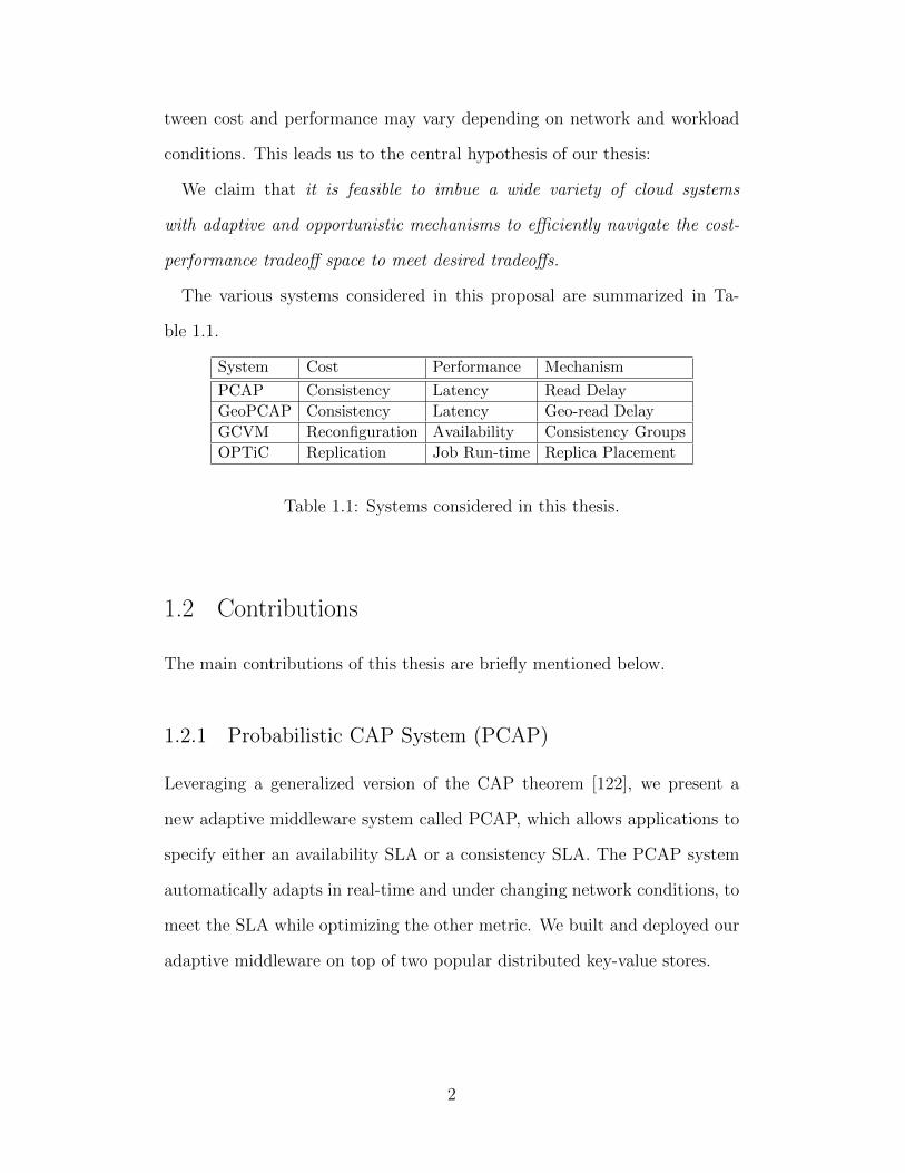
The various systems considered in this proposal are summarized in Ta-

ble 1.1.

System Cost Performance Mechanism

PCAP Consistency Latency Read Delay

GeoPCAP Consistency Latency Geo-read Delay

GCVM Reconfiguration Availability Consistency Groups

OPTiC Replication Job Run-time Replica Placement

Table 1.1: Systems considered in this thesis.

1.2 Contributions

The main contributions of this thesis are briefly mentioned below.

1.2.1 Probabilistic CAP System (PCAP)

Leveraging a generalized version of the CAP theorem [122], we present a

new adaptive middleware system called PCAP, which allows applications to

specify either an availability SLA or a consistency SLA. The PCAP system

automatically adapts in real-time and under changing network conditions, to

meet the SLA while optimizing the other metric. We built and deployed our

adaptive middleware on top of two popular distributed key-value stores.

2

1.2.2 Geo-distributed PCAP (GeoPCAP)

We develop a theoretical framework for probabilistically composing consis-

tency and latency models of multiple distributed storage systems running

across geo-distributed datacenters. Using this framework, we also design

and implement a geo-distributed adaptive system to meet consistency-latency

(PCAP) SLAs.

1.2.3 Software-defined Group Consistent Snapshots for VMs(GCVM)

For a hardware storage array, a consistency group is defined as a group of

devices that can be checkpointed and replicated as a group [12]. We propose

to move consistency group abstractions from hardware to software. This

allows increased flexibility for defining consistency groups for checkpointing

and replication. It also reduces the cost of reconfiguring consistency groups,

which can now be done at the hypervisor level. However this approach incurs

the cost of pausing the VM pause leading to increased application unavail-

ability. Our implemented mechanism correctly takes crash-consistent snap-

shots of a group of VMs, while keeping the VM pause overhead bounded by

50 msec. With some constraints on application write ordering, we demon-

strate that this approach can be used to recover real applications without

complicated distributed snapshot algorithms or coordination.

1.2.4 Opportunistic Graph Processing in Multi-tenantClusters (OPTiC)

We investigate for the first time how multiple graph analytics jobs sharing a

cluster can improve overall job performance by trading the additional storage

3

and bandwidth cost of one more replica of the input graph data. The place-

ment of the additional replica is opportunistically selected based on novel

progress metrics for current running graph analytics jobs. We incorporated

our system on top of Apache Giraph running on Apache YARN in conjunc-

tion with HDFS. Our deployment experiments under realistic network and

workload conditions show around 40% performance improvement in average

job completion time, at the cost of increased data replication.

1.3 Cost-Performance Tradeoffs as First Class Citizens

for Cloud Systems

A central tenet of this thesis is that we should consider cost-performance

tradeoffs as first class citizens when designing cloud systems. Today many

cloud systems are designed with only an explicit goal of either optimizing

performance or minimizing cost, but not both. Explicitly mapping out the

cost performance tradeoff space for cloud systems allows us to better design

and reason about cloud systems in the following ways:

1. It allows us to characterize the optimal tradeoff (PCAP, Chapter 2), or

conjecture what the optimal tradeoff can look like (OPTiC, Chapter 5).

2. It allows us to think of future designs of the same system with new

tradeoffs in the tradeoff space, and predict cost and performance for

such designs (GCVM, Chapter 4).

These points are discussed in further detail at the end of this thesis in

Chapter 6.

4

1.4 Thesis Organization

The rest of the thesis is organized as follows. Chapter 2 presents the de-

sign, implementation, and evaluation of PCAP, an adaptive distributed stor-

age system for meeting novel probabilistic consistency/latency SLAs for ap-

plications running inside a data-center under realistic network conditions.

Chapter 3 presents GeoPCAP, which is a geo-distributed extension of PCAP

(Chapter 2). Chapter 4 presents the design and evaluation of GCVM, which

is a hypervisor-managed system for implementing consistency group abstrac-

tions for a group of virtual machines. Chapter 5 discusses the design, imple-

mentation and evaluation of OPTiC, a system to opportunistically schedule

graph processing jobs in a shared multi-tenant cluster. Finally we summarize

and discuss future directions in Chapter 6.

5

Chapter 2

PCAP: Characterizing and Adapting theConsistency-Latency Tradeoff for Distributed

Key-Value Stores

In this chapter we present our system PCAP. PCAP is based on a new proba-

bilistic characterization of the consistency-latency tradeoffs for a distributed

key-value store [123]. PCAP leverages adaptive techniques to meet novel

consistency-latency SLAs under varying network conditions in a data-center

network. We have incorporated our PCAP system design on top of two

popular open-source key-value stores: Apache Cassandra and Basho Riak.

Deployment experiments confirm that PCAP can meet probabilistic consis-

tency and latency SLAs under network variations within a single data-center

environment.

2.1 Introduction

Storage systems form the foundational platform for modern Internet ser-

vices such as Web search, analytics, and social networking. Ever increasing

user bases and massive data sets have forced users and applications to forgo

conventional relational databases, and move towards a new class of scalable

storage systems known as NoSQL key-value stores. Many of these distributed

key-value stores (e.g., Cassandra [8], Riak [7], Dynamo [71], Voldemort [24])

support a simple GET/PUT interface for accessing and updating data items.

The data items are replicated at multiple servers for fault tolerance. In addi-

tion, they offer a very weak notion of consistency known as eventual consis-

6

tency [139, 48], which roughly speaking, says that if no further updates are

sent to a given data item, all replicas will eventually hold the same value.

These key-value stores are preferred by applications for whom eventual

consistency suffices, but where high availability and low latency (i.e., fast

reads and writes [40]) are paramount. Latency is a critical metric for such

cloud services because latency is correlated to user satisfaction – for instance,

a 500 ms increase in latency for operations at Google.com can cause a 20%

drop in revenue [1]. At Amazon, this translates to a $6M yearly loss per

added millisecond of latency [2]. This correlation between delay and lost

retention is fundamentally human. Humans suffer from a phenomenon called

user cognitive drift, wherein if more than a second (or so) elapses between

clicking on something and receiving a response, the user’s mind is already

elsewhere.

At the same time, clients in such applications expect freshness, i.e., data

returned by a read to a key should come from the latest writes done to that

key by any client. For instance, Netflix uses Cassandra to track positions in

each video [66], and freshness of data translates to accurate tracking and user

satisfaction. This implies that clients care about a time-based notion of data

freshness. Thus, this chapter focuses on consistency based on the notion of

data freshness (as defined later).

The CAP theorem was proposed by Brewer et al. [57, 56], and later for-

mally proved by [78, 108]. It essentially states that a system can choose

at most two of three desirable properties: Consistency (C), Availability (A),

and Partition tolerance (P). Recently, [40] proposed to study the consistency-

latency tradeoff, and unified the tradeoff with the CAP theorem. The unified

result is called PACELC. It states that when a network partition occurs, one

needs to choose between Availability and Consistency, otherwise the choice

7

is between Latency and Consistency. We focus on the latter tradeoff as it is

the common case. These prior results provided qualitative characterization

of the tradeoff between consistency and availability/latency, while we provide

a quantitative characterization of the tradeoff.

Concretely, traditional CAP literature tends to focus on situations where

“hard” network partitions occur and the designer has to choose between C

or A, e.g., in geo-distributed data-centers. However, individual data-centers

themselves suffer far more frequently from “soft” partitions [70], arising from

periods of elevated message delays or loss rates (i.e., the “otherwise” part of

PACELC) within a data-center. Neither the original CAP theorem nor the

existing work on consistency in key-value stores [50, 71, 80, 88, 102, 105, 106,

130, 135, 139] address such soft partitions for a single data-center.

In this chapter we state and prove two CAP-like impossibility theorems.

To state these theorems, we present probabilistic1 models to characterize the

three important elements: soft partition, latency requirements, and consis-

tency requirements. All our models take timeliness into account. Our latency

model specifies soft bounds on operation latencies, as might be provided by

the application in an SLA (Service Level Agreement). Our consistency model

captures the notion of data freshness returned by read operations. Our par-

tition model describes propagation delays in the underlying network. The

resulting theorems show the un-achievable envelope, i.e., which combinations

of the parameters in these three models (partition, latency, consistency) make

them impossible to achieve together. Note that the focus of the chapter is

neither defining a new consistency model nor comparing different types of

consistency models. Instead, we are interested in the un-achievable enve-

lope of the three important elements and measuring how close a system can

1By probabilistic, we mean the behavior is statistical over a long time period.

8

perform to this envelop.

Next, we describe the design of a class of systems called PCAP (short for

Probabilistic CAP) that perform close to the envelope described by our the-

orems. In addition, these systems allow applications running inside a single

data-center to specify either a probabilistic latency SLA or a probabilistic

consistency SLA. Given a probabilistic latency SLA, PCAP’s adaptive tech-

niques meet the specified operational latency requirement, while optimizing

the consistency achieved. Similarly, given a probabilistic consistency SLA,

PCAP meets the consistency requirement while optimizing operational la-

tency. PCAP does so under real and continuously changing network condi-

tions. There are known use cases that would benefit from an latency SLA

– these include the Netflix video tracking application [66], online advertis-

ing [26], and shopping cart applications [135] – each of these needs fast re-

sponse times but is willing to tolerate some staleness. A known use case

for consistency SLA is a Web search application [135], which desires search

results with bounded staleness but would like to minimize the response time.

While the PCAP system can be used with a variety of consistency and latency

models (like PBS [50]), we use our PCAP models for concreteness.

We have integrated our PCAP system into two key-value stores – Apache

Cassandra [8] and Riak [7]. Our experiments with these two deployments,

using YCSB [67] benchmarks, reveal that PCAP systems satisfactorily meets

a latency SLA (or consistency SLA), optimize the consistency metric (respec-

tively latency metric), perform reasonably close to the envelope described by

our theorems, and scale well.

9

2.2 Consistency-Latency Tradeoff

We consider a key-value store system which provides a read/write API over

an asynchronous distributed message-passing network. The system consists

of clients and servers, in which, servers are responsible for replicating the data

(or read/write object) and ensuring the specified consistency requirements,

and clients can invoke a write (or read) operation that stores (or retrieves)

some value of the specified key by contacting server(s). We assume each

client has a corresponding client proxy at the set of servers, which submits

read and write operations on behalf of clients [105, 129]. Specifically, in the

system, data can be propagated from a writer client to multiple servers by a

replication mechanism or background mechanism such as read repair [71], and

the data stored at servers can later be read by clients. There may be multiple

versions of the data corresponding to the same key, and the exact value to

be read by reader clients depends on how the system ensures the consistency

requirements. Note that as addressed earlier, we define consistency based on

freshness of the value returned by read operations (defined below). We first

present our probabilistic models for soft partition, latency and consistency.

Then we present our impossibility results. These results only hold for a single

data-center. Later in Section 3 we deal with the multiple data-center case.

2.2.1 Models

To capture consistency, we defined a new notion called t-freshness, which is

a form of eventual consistency. Consider a single key (or read/write object)

being read and written concurrently by multiple clients. An operation O

(read or write) has a start time τstart(O) when the client issues O, and a

finish time τfinish(O) when the client receives an answer (for a read) or an

10

acknowledgment (for a write). The write operation ends when the client

receives an acknowledgment from the server. The value of a write operation

can be reflected on the server side (i.e., visible to other clients) any time

after the write starts. For clarity of our presentation, we assume that all

write operations end, which is reasonable given client retries. Note that the

written value can still propagate to other servers after the write ends by the

background mechanism.We assume that at time 0 (initial time), the key has

a default value.

Definition 1 t-freshness and t-staleness: A read operation R is said to

be t-fresh if and only if R returns a value written by any write operation that

starts at or after time τfresh(R, t), which is defined below:

1. If there is at least one write starting in the interval [τstart(R)−t, τstart(R)]:

then τfresh(R, t) = τstart(R)− t.

2. If there is no write starting in the interval [τstart(R)− t, τstart(R)], then

there are two cases:

(a) No write starts before R starts: then τfresh(R, t) = 0.

(b) Some write starts before R starts: then τfresh(R, t) is the start

time of the last write operation that starts before τstart(R)− t.

A read that is not t-fresh is said to be t-stale.

Note that the above characterization of tfresh(R, t) only depends on start

times of operations.

Fig. 2.1 shows three examples for t-freshness. The figure shows the times at

which several read and write operations are issued (the time when operations

complete are not shown in the figure). W (x) in the figure denotes a write

11

Figure 2.1: Examples illustrating Definition 1. Only start times of eachoperation are shown.

operation with a value x. Note that our definition of t-freshness allows a read

to return a value that is written by a write issued after the read is issued.

In Fig. 2.1(i), τfresh(R, t) = τstart(R)− t = t′ − t; therefore, R is t-fresh if it

returns 2, 3 or 4. In Fig. 2.1(ii), τfresh(R, t) = τstart(W (1)); therefore, R is

t-fresh if it returns 1, 4 or 5. In Fig. 2.1(iii), τfresh(R, t) = 0; therefore, R is

t-fresh if it returns 4, 5 or the default.

Definition 2 Probabilistic Consistency: A key-value store satisfies (tc, pic)-

consistency2 if in any execution of the system, the fraction of read operations

satisfying tc-freshness is at least (1− pic).

Intuitively, pic is the likelihood of returning stale data,

given the time-based freshness requirement tc.

Two similar definitions have been proposed previously: (1) t-visibility from

the Probabilistically Bounded Staleness (PBS) work [50], and (2) ∆-atomicity

[81]. These two metrics do not require a read to return the latest write, but

provide a time bound on the staleness of the data returned by the read.

The main difference between t-freshness and these is that we consider the

2The subscripts c and ic stand for consistency and inconsistency, respectively.

12

start time of write operations rather than the end time. This allows us to

characterize consistency-latency tradeoff more precisely. While we prefer t-

freshness, our PCAP system (Section 2.3) is modular and could use instead

t-visibility or ∆-atomicity for estimating data freshness.

As noted earlier, our focus is not comparing different consistency models,

nor achieving linearizability. We are interested in the un-achievable enve-

lope of soft partition, latency requirements, and consistency requirements.

Traditional consistency models like linearizability can be achieved by delay-

ing the effect of a write. On the contrary, the achievability of t-freshness

closely ties to the latency of read operations and underlying network behav-

ior as discussed later. In other words, t-freshness by itself is not a complete

definition.

2.2.2 Use Case for t − freshness

Consider a bidding application (e.g., eBay), where everyone can post a bid,

and we want every other participant to see posted bids as fast as possible.

Assume that User 1 submits a bid, which is implemented as a write request

(Figure 2.2). User 2 requests to read the bid before the bid write process fin-

ishes. The same User 2 then waits a finite amount of time after the bid write

completes and submits another read request. Both of these read operations

must reflect User 1’s bid, whereas t-visibility only reflects the write in User

2’s second read (with suitable choice of t). The bid write request duration

can include time to send back an acknowledgment to the client, even after

the bid has committed (on the servers). A client may not want to wait that

long to see a submitted bid. This is especially true when the auction is near

the end.

13

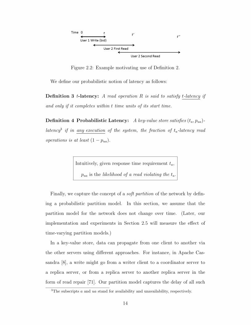
Figure 2.2: Example motivating use of Definition 2.

We define our probabilistic notion of latency as follows:

Definition 3 t-latency: A read operation R is said to satisfy t-latency if

and only if it completes within t time units of its start time.

Definition 4 Probabilistic Latency: A key-value store satisfies (ta, pua)-

latency3 if in any execution of the system, the fraction of ta-latency read

operations is at least (1− pua).

Intuitively, given response time requirement ta,

pua is the likelihood of a read violating the ta.

Finally, we capture the concept of a soft partition of the network by defin-

ing a probabilistic partition model. In this section, we assume that the

partition model for the network does not change over time. (Later, our

implementation and experiments in Section 2.5 will measure the effect of

time-varying partition models.)

In a key-value store, data can propagate from one client to another via

the other servers using different approaches. For instance, in Apache Cas-

sandra [8], a write might go from a writer client to a coordinator server to

a replica server, or from a replica server to another replica server in the

form of read repair [71]. Our partition model captures the delay of all such

3The subscripts a and ua stand for availability and unavailability, respectively.

14

propagation approaches. Please note that the partition model applies not to

the network directly, but to the paths taken by the read or write operation

queries themselves. This means that the network as a whole may be good

(or bad), but if the paths taken by the queries are bad (or good), only the

latter matters.

Definition 5 Probabilistic Partition:

An execution is said to suffer (tp, α)-partition if the fraction f of paths

from one client to another client, via a server, which have latency higher

than tp, is such that f ≥ α.

Our delay model loosely describes the message delay caused by any un-

derlying network behavior without relying on the assumptions on the im-

plementation of the key-value store. We do not assume eventual delivery of

messages. We neither define propagation delay for each message nor specify

the propagation paths (or alternatively, the replication mechanisms). This

is because we want to have general lower bounds that apply to all systems

that satisfy our models.

2.2.3 Impossibility Results

We now present two theorems that characterize the consistency-latency trade-

off in terms of our probabilistic models.4

First, we consider the case when the client has tight expectations, i.e., the

client expects all data to be fresh within a time bound, and all reads need to

be answered within a time bound.

4These impossibility results are not a contribution of this thesis. They were discoveredindependently by Lewis Tseng and Indranil Gupta. Since they form the foundation of ourPCAP system (which is a contribution of this thesis), we include the results here only asbackground material.)

15

Theorem 1 If tc + ta < tp, then it is impossible to implement a read/write

data object under a (tp, 0)-partition while achieving (tc, 0)-consistency, and

(ta, 0)-latency, i.e., there exists an execution such that these three properties

cannot be satisfied simultaneously.

Proof: The proof is by contradiction. In a system that satisfies all three

properties in all executions, consider an execution with only two clients, a

writer client and a reader client. There are two operations: (i) the writer

client issues a write W , and (ii) the reader client issues a read R at time

τstart(R) = τstart(W ) + tc. Due to (tc, 0)-consistency, the read R must return

the value from W .

Let the delay of the write request W be exactly tp units of time (this obeys

(tp, 0)-partition). Thus, the earliest time that W ’s value can arrive at the

reader client is (τstart(W )+ tp). However, to satisfy (ta, 0)-latency, the reader

client must receive an answer by time τstart(R) + ta = τstart(W ) + tc + ta.

However, this time is earlier than (τstart(W ) + tp) because tc + ta < tp.

Hence, the value returned by W cannot satisfy (tc, 0)-consistency. This is a

contradiction. 2

Essentially, the above theorem relates the clients’ expectations of freshness

(tc) and latency (ta) to the propagation delays (tp). If client expectations are

too stringent when the maximum propagation delay is large, then it may not

be possible to guarantee both consistency and latency expectations.

However, if we allow a fraction of the reads to return late (i.e., after ta), or

return tc-stale values (i.e., when either pic or pua is non-zero), then it may be

possible to satisfy the three properties together even if tc + ta < tp. Hence,

we consider non-zero pic, pua and α in our second theorem.

16

Theorem 2 If tc + ta < tp, and pua + pic < α, then it is impossi-

ble to implement a read/write data object under a (tp, α)-partition while

achieving (tc, pic)-consistency, and (ta, pua)-latency, i.e., there exists an ex-

ecution such that these three properties cannot be satisfied simultaneously.

Proof: The proof is by contradiction. In a system that satisfies all three

properties in all executions, consider an execution with only two clients, a

writer client and a reader client. The execution contains alternating pairs of

write and read operations W1, R1,W2, R2, . . . ,Wn, Rn, such that:

• Write Wi starts at time (tc + ta) · (i− 1),

• Read Ri starts at time (tc + ta) · (i− 1) + tc, and

• Each write Wi writes a distinct value vi.

By our definition of (tp, α)-partition, there are at least n ·α written values

vj’s that have propagation delay > tp. By a similar argument as in the proof

of Theorem 1, each of their corresponding reads Rj are such that Rj cannot

both satisfy tc-freshness and also return within ta. That is, Rj is either tc-

stale or returns later than ta after its start time. There are n · α such reads

Rj; let us call these “bad” reads.

By definition, the set of reads S that are tc-stale, and the set of reads A

that return after ta are such that |S| ≤ n ·pic and |A| ≤ n ·pua. Put together,

these imply:

n · α ≤ |S ∪ A| ≤ |S|+ |A| ≤ n · pic + n · pua.

The first inequality arises because all the “bad” reads are in S ∪ A. But

this inequality implies that α ≤ pua + pic, which violates our assumptions. 2

The intuition behind the theorem is as follows. As network conditions

worsen, the values for (α, tp) go up. On the other hand a client can get better

freshness (latency) for reads by lowering the values of (pic,tc) ((pua, ta)). Thus

17

high values for (α, tp) prevent the values for (pic,tc), and (pua, ta) to be arbi-

trarily small. The inequalities thus represent the best freshness (pic,tc) and

latency (pua, ta) combinations for a given network characterized by (α, tp).

2.3 PCAP Key-value Stores

Having formally specified the (un)achievable envelope of consistency-latency

(Theorem 2), we now move our attention to designing systems that achieve

performance close to this theoretical envelope. We also convert our prob-

abilistic models for consistency and latency from Section 2.2 into SLAs,

and show how to design adaptive key-value stores that satisfy such prob-

abilistic SLAs inside a single data-center. We call such systems PCAP sys-

tems. So PCAP systems (1) can achieve performance close to the theoretical

consistency-latency tradeoff envelope, and (2) can adapt to meet probabilistic

consistency and latency SLAs inside a single data-center. Our PCAP systems

can also alternatively be used with SLAs from PBS [50] or Pileus [45, 135].

Assumptions about underlying Key-value Store PCAP systems can

be built on top of existing key-value stores. We make a few assumptions

about such key-value stores. First, we assume that each key is replicated on

multiple servers. Second, we assume the existence of a “coordinator” server

that acts as a client proxy in the system, finds the replica locations for a

key (e.g., using consistent hashing [134]), forwards client queries to replicas,

and finally relays replica responses to clients. Most key-value stores feature

such a coordinator [7, 8]. Third, we assume the existence of a background

mechanism such as read repair [71] for reconciling divergent replicas. Finally,

we assume that the clocks on each server in the system are synchronized using

18

a protocol like NTP so that we can use global timestamps to detect stale

data (most key-value stores running within a datacenter already require this

assumption, e.g., to decide which updates are fresher). It should be noted

that our impossibility results in Section 2.2 do not depend on the accuracy of

the clock synchronization protocol. However the sensitivity of the protocol

affects the ability of PCAP systems to adapt to network delays. For example,

if the servers are synchronized to within 1 ms using NTP, then the PCAP

system cannot react to network delays lower than 1 ms.

SLAs We consider two scenarios, where the SLA specifies either: i) a prob-

abilistic latency requirement, or ii) a probabilistic consistency requirement.

In the former case, our adaptive system optimizes the probabilistic consis-

tency while meeting the SLA requirement, whereas in the latter it optimizes

probabilistic latency while meeting the SLA. These SLAs are probabilistic,

in the sense that they give statistical guarantees to operations over a long

duration.

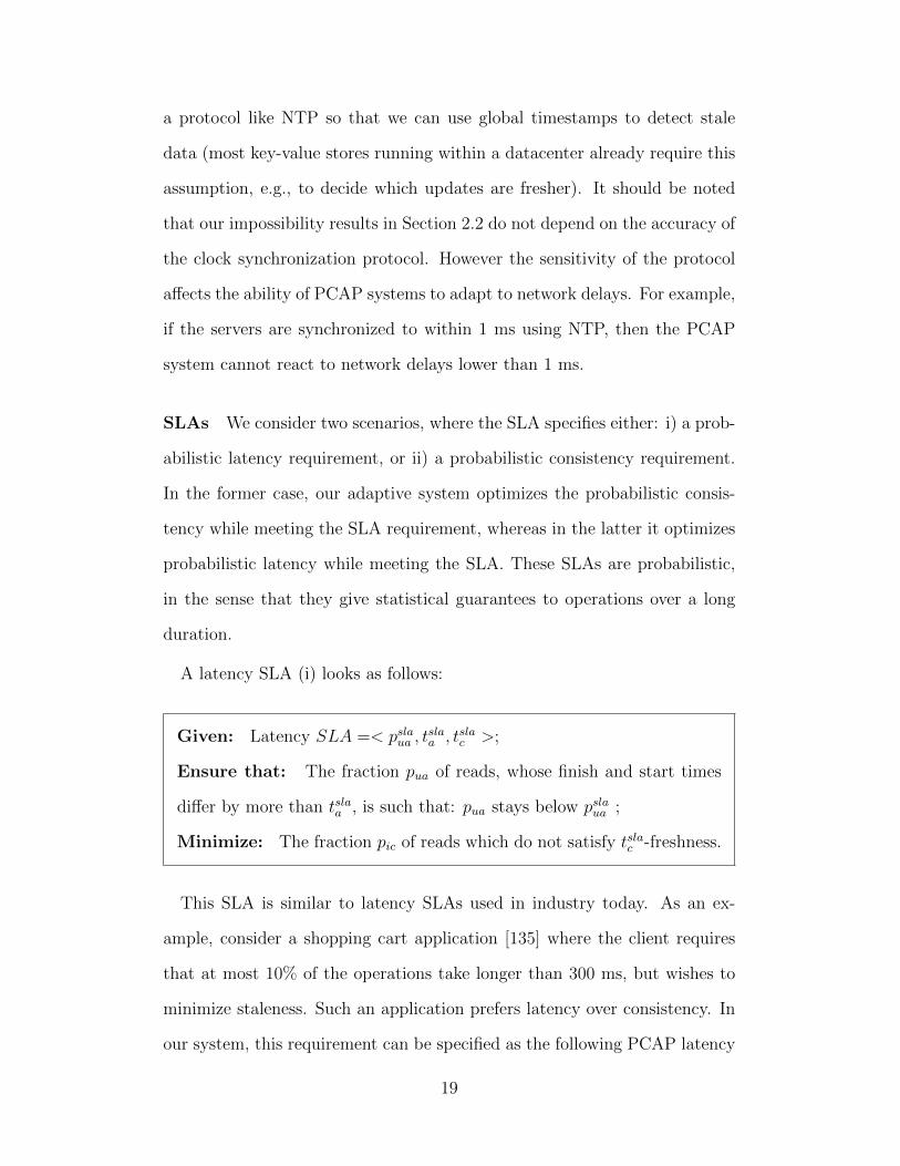
A latency SLA (i) looks as follows:

Given: Latency SLA =< pslaua , tslaa , tslac >;

Ensure that: The fraction pua of reads, whose finish and start times

differ by more than tslaa , is such that: pua stays below pslaua ;

Minimize: The fraction pic of reads which do not satisfy tslac -freshness.

This SLA is similar to latency SLAs used in industry today. As an ex-

ample, consider a shopping cart application [135] where the client requires

that at most 10% of the operations take longer than 300 ms, but wishes to

minimize staleness. Such an application prefers latency over consistency. In

our system, this requirement can be specified as the following PCAP latency

19

SLA:

< pslaua , tslaa , tslac >=< 0.1, 300 ms, 0 ms >.

A consistency SLA looks as follows:

Given: Consistency SLA =< pslaic , tslaa , tslac >;

Ensure that: The fraction pic of reads that do not satisfy tslac -freshness

is such that: pic stays below pslaic ;

Minimize: The fraction pua of reads whose finish and start times differ

by more than tslaa .

Note that as mentioned earlier, consistency is defined based on freshness

of the value returned by read operations. As an example, consider a web

search application that wants to ensure no more than 10% of search results

return data that is over 500 ms old, but wishes to minimize the fraction

of operations taking longer than 100 ms [135]. Such an application prefers

consistency over latency. This requirement can be specified as the following

PCAP consistency SLA:

< pslaic , tslaa , tslac >=< 0.10, 100 ms, 500 ms >.

Our PCAP system can leverage three control knobs to meet these SLAs:

1) read delay, 2) read repair rate, and 3) consistency level. The last two of

these are present in most key-value stores. The first (read delay) has been

discussed in previous literature [10, 50, 75, 83, 145].

2.3.1 Control Knobs

Table 2.1 shows the effect of our three control knobs on latency and consis-

tency. We discuss each of these knobs and explain the entries in the table.

The knobs of Table 2.1 are all directly or indirectly applicable to the read

20

Increased Knob Latency Consistency

Read Delay Degrades ImprovesRead Repair Rate Unaffected ImprovesConsistency Level Degrades Improves

Table 2.1: Effect of Various Control Knobs.

path in the key-value store. As an example, the knobs pertaining to the

Cassandra query path are shown in Fig. 2.3, which shows the four major

steps involved in answering a read query from a front-end to the key-value

store cluster: (1) Client sends a read query for a key to a coordinator server

in the key-value store cluster; (2) Coordinator forwards the query to one

or more replicas holding the key; (3) Response is sent from replica(s) to

coordinator; (4) Coordinator forwards response with highest timestamp to

client; (5) Coordinator does read repair by updating replicas, which had

returned older values, by sending them the freshest timestamp value for the

key. Step (5) is usually performed in the background.

Figure 2.3: Cassandra Read Path and PCAP Control Knobs.

A read delay involves the coordinator artificially delaying the read query for

a specified duration of time before forwarding it to the replicas. i.e., between

step (1) and step (2). This gives the system some time to converge after pre-

21

vious writes. Increasing the value of read delay improves consistency (lowers

pic) and degrades latency (increases pua). Decreasing read delay achieves the

reverse. Read delay is an attractive knob because: 1) it does not interfere

with client specified parameters (e.g., consistency level in Cassandra), and 2)

it can take any non-negative continuous value instead of only discrete values

allowed by consistency levels. Our PCAP system inserts read delays only

when it is needed to satisfy the specified SLA.

However, read delay cannot be negative, as one cannot speed up a query

and send it back in time. This brings us to our second knob: read repair

rate. Read repair was depicted as distinct step (5) in our outline of Fig. 2.3,

and is typically performed in the background. The coordinator maintains a

buffer of recent reads where some of the replicas returned older values along

with the associated freshest value. It periodically picks an element from this

buffer and updates the appropriate replicas. In key-value stores like Apache

Cassandra and Riak, read repair rate is an accessible configuration parameter

per column family.

Our read repair rate knob is the probability with which a given read that

returned stale replica values will be added to the read repair buffer. Thus,

a read repair rate of 0 implies no read repair, and replicas will be updated

only by subsequent writes. Read repair rate = 0.1 means the coordinator

performs read repair for 10% of the read requests.

Increasing (respectively, decreasing) the read repair rate can improve (re-

spectively degrade) consistency. Since the read repair rate does not directly

affect the read path (Step (5) described earlier, is performed in the back-

ground), it does not affect latency. Table 2.1 summarizes this behavior.5

5Although read repair rate does not affect latency directly, it introduces some back-ground traffic and can impact propagation delay. While our model ignores such smallimpacts, our experiments reflect the net effect of the background traffic.

22

The third potential control knob is consistency level. Some key-value stores

allow the client to specify, along with each read or write operation, how many

replicas the coordinator should wait for (in step (3) of Fig. 2.3) before it sends

the reply back in step (4). For instance, Cassandra offers consistency levels:

ONE, TWO, QUORUM, ALL. As one increases consistency level from ONE to ALL,

reads are delayed longer (latency decreases) while the possibility of returning

the latest write rises (consistency increases).

Our PCAP system relies primarily on read delay and repair rate as the

control knobs. Consistency level can be used as a control knob only for ap-

plications in which user expectations will not be violated, e.g., when reads

do not specify a specific discrete consistency level. That is, if a read specifies

a higher consistency level, it would be prohibitive for the PCAP system to

degrade the consistency level as this may violate client expectations. Tech-

niques like continuous partial quorums (CPQ) [113], and adaptive hybrid

quorums [69] fall in this category, and thus interfere with application/client

expectations. Further, read delay and repair rate are non-blocking control

knobs under replica failure, whereas consistency level is blocking. For exam-

ple, if a Cassandra client sets consistency level to QUORUM with replication

factor 3, then the coordinator will be blocked if two of the key’s replicas are

on failed nodes. On the other hand, under replica failures read repair rate

does not affect operation latency, while read delay only delays reads by a

maximum amount.

2.3.2 Selecting A Control Knob

As the primary control knob, the PCAP system prefers read delay over read

repair rate. This is because the former allows tuning both consistency and

23

latency, while the latter affects only consistency. The only exception occurs

when during the PCAP system adaptation process, a state is reached where

consistency needs to be degraded (e.g., increase pic to be closer to the SLA)

but the read delay value is already zero. Since read delay cannot be lowered

further, in this instance the PCAP system switches to using the secondary

knob of read repair rate, and starts decreasing this instead.

Another reason why read repair rate is not a good choice for the primary

knob is that it takes longer to estimate pic than for read delay. Because read

repair rate is a probability, the system needs a larger number of samples

(from the operation log) to accurately estimate the actual pic resulting from

a given read repair rate. For example, in our experiments, we observe that

the system needs to inject k ≥ 3000 operations to obtain an accurate estimate

of pic, whereas only k = 100 suffices for the read delay knob.

2.3.3 PCAP Control Loop

The PCAP control loop adaptively tunes control knobs to always meet the

SLA under continuously changing network conditions. The control loop for

consistency SLA is depicted in Fig. 2.4. The control loop for a latency SLA

is analogous and is not shown.

This control loop runs at a standalone server called the PCAP Coordina-

tor.6 This server runs an infinite loop. In each iteration, the coordinator:

i) injects k operations into the store (line 6), ii) collects the log L for the k

recent operations in the system (line 8), iii) calculates pua, pic (Section 2.3.4)

from L (line 10), and iv) uses these to change the knob (lines 12-22).

The behavior of the control loop in Fig. 2.4 is such that the system will

6The PCAP Coordinator is a special server, and is different from Cassandra’s use of acoordinator for clients to send reads and writes.

24

1: procedure control(SLA =< pslaic , tslac , tslaa >, ε)

2: psla′

ic := pslaic − ε;3: Select control knob; // (Sections 2.3.1, 2.3.2)4: inc := 1;5: dir = +1;6: while (true) do7: Inject k new operations (reads and writes)8: into store;9: Collect log L of recent completed reads

10: and writes (values, start and finish times);11: Use L to calculate12: pic and pua; // (Section 2.3.4)13: new dir := (pic > psla

′ic )? + 1 : −1;

14: if new dir = dir then15: inc := inc ∗ 2; // Multiplicative increase16: if inc > MAX INC then17: inc := MAX INC:18: end if19: else20: inc := 1; // Reset to unit step21: dir := new dir; // Change direction22: end if23: control knob := control knob+ inc ∗ dir;24: end while25: end procedure

Figure 2.4: Adaptive Control Loop for Consistency SLA.

converge to “around” the specified SLA. Because our original latency (con-

sistency) SLAs require pua (pic) to stay below the SLA, we introduce a lax-

ity parameter ε, subtract ε from the target SLA, and treat this as the tar-

get SLA in the control loop. Concretely, given a target consistency SLA

< pslaic , tslaa , tslac >, where the goal is to control the fraction of stale reads to

be under pslaic , we control the system such that pic quickly converges around

psla′

ic = pslaic −ε, and thus stay below pslaic . Small values of ε suffice to guarantee

convergence (for instance, our experiments use ε ≤ 0.05).

We found that the naive approach of changing the control knob by the

smallest unit increment (e.g., always 1 ms changes in read delay) resulted

25

in a long convergence time. Thus, we opted for a multiplicative approach

(Fig. 2.4, lines 12-22) to ensure quick convergence.

We explain the control loop via an example. For concreteness, suppose

only the read delay knob (Section 2.3.1) is active in the system, and that

the system has a consistency SLA. Suppose pic is higher than psla′

ic . The

multiplicative-change strategy starts incrementing the read delay, initially

starting with a unit step size (line 3). This step size is exponentially in-

creased from one iteration to the next, thus multiplicatively increasing read

delay (line 14). This continues until the measured pic goes just under psla′

ic .

At this point, the new dir variable changes sign (line 12), so the strategy re-

verses direction, and the step is reset to unit size (lines 19-20). In subsequent

iterations, the read delay starts decreasing by the step size. Again, the step

size is increased exponentially until pic just goes above psla′

ic . Then its direc-

tion is reversed again, and this process continues similarly thereafter. Notice

that (lines 12-14) from one iteration to the next, as long as pic continues to

remain above (or below) psla′

ic , we have that: i) the direction of movement

does not change, and ii) exponential increase continues. At steady state, the

control loop keeps changing direction with a unit step size (bounded oscil-

lation), and the metric stays converged under the SLA. Although advanced

techniques such as time dampening can further reduce oscillations, we de-

cided to avoid them to minimize control loop tuning overheads. Later in

Chapter 3, we utilized control theoretic techniques for the control loop in

geo-distributed settings to reduce excessive oscillations.

In order to prevent large step sizes, we cap the maximum step size (line

15-17). For our experiments, we do not allow read delay to exceed 10 ms,

and the unit step size is set to 1 ms.

We preferred active measurement (whereby the PCAP Coordinator injects

26

queries rather than passive due to two reasons: i) the active approach gives

the PCAP Coordinator better control on convergence, thus convergence rate

is more uniform over time, and ii) in the passive approach if the client op-

eration rate were to become low, then either the PCAP Coordinator would

need to inject more queries, or convergence would slow down. Neverthe-

less, in Section 2.5.3, we show results using a passive measurement approach.

Exploration of hybrid active-passive approaches based on an operation rate

threshold could be an interesting direction.

Overall our PCAP controller satisfies SASO (Stability, Accuracy, low Set-

tling time, small Overshoot) control objectives [87].

2.3.4 Complexity of Computing pua and pic

We show that the computation of pua and pic (line 10, Fig. 2.4) is efficient.

Suppose there are r reads and w writes in the log, thus log size k = r + w.

Calculating pua makes a linear pass over the read operations, and compares

the difference of their finish and start times with ta. This takes O(r) = O(k).

pic is calculated as follows. We first extract and sort all the writes according

to start timestamp, inserting each write into a hash table under key <object

value, write key, write timestamp>. In a second pass over the read opera-

tions, we extract its matching write by using the hash table key (the third

entry of the hash key is the same as the read’s returned value timestamp).

We also extract neighboring writes of this matching write in constant time

(due to the sorting), and thus calculate tc-freshness for each read. The first

pass takes time O(r+w+w logw), while the second pass takes O(r+w). The

total time complexity to calculate pic is thus O(r+w+w logw) = O(k log k).

27

2.4 Implementation Details

In this section, we discuss how support for our consistency and latency SLAs

can be easily incorporated into the Cassandra and Riak key-value stores (in

a single data-center) via minimal changes.

2.4.1 PCAP Coordinator

From Section 2.3.3, recall that the PCAP Coordinator runs an infinite loop

that continuously injects operations, collects logs (k = 100 operations by

default), calculates metrics, and changes the control knob. We implemented

a modular PCAP Coordinator using Python (around 100 LOC), which can

be connected to any key-value store.

We integrated PCAP into two popular NoSQL stores: Apache Cassan-

dra [8] and Riak [7] – each of these required changes to about 50 lines of

original store code.7

2.4.2 Apache Cassandra

First, we modified the Cassandra v1.2.4 to add read delay and read repair

rate as control knobs. We changed the Cassandra Thrift interface so that it

accepts read delay as an additional parameter. Incorporating the read delay

into the read path required around 50 lines of Java code.

Read repair rate is specified as a column family configuration parameter,

and thus did not require any code changes. We used YCSB’s Cassandra

connector as the client, modified appropriately to talk with the clients and

7The implementation of PCAP on top of Riak is not a contribution of this thesis.This implementation was done by Son Nguyen under the guidance of the author of thisthesis. The design of PCAP Riak closely follows the design of PCAP Cassandra which isa contribution of this thesis.

28

the PCAP Coordinator.

2.4.3 Riak

We modified Riak v1.4.2 to add read delay and read repair as control knobs.

Due to the unavailability of a YCSB Riak connector, we wrote a separate

YCSB client for Riak from scratch (250 lines of Java code). We decided to use

YCSB instead of existing Riak clients, since YCSB offers flexible workload

choices that model real world key-value store workloads.

We introduced a new system-wide parameter for read delay, which was

passed via the Riak http interface to the Riak coordinator which in turn

applied it to all queries that it receives from clients. This required about 50

lines of Erlang code in Riak. Like Cassandra, Riak also has built-in support

for controlling read repair rate.

2.5 Experiments

Our experiments are in two stages: microbenchmarks for a single data-center

(Section 2.5.2) and deployment experiments for a single data-center (Sec-

tion 2.5.3).

2.5.1 Experiment Setup

Our single data-center PCAP Cassandra system and our PCAP Riak system

were each run with their default settings. We used YCSB v 0.1.4 [36] to

send operations to the store. YCSB generates synthetic workloads for key-

value stores and models real-world workload scenarios (e.g., Facebook photo

storage workload). It has been used to benchmark many open-source and

29

commercial key-value stores, and is the de facto benchmark for key-value

stores [67].

Each YCSB experiment consisted of a load phase, followed by a work

phase. Unless otherwise specified, we used the following YCSB parameters:

16 threads per YCSB instance, 2048 B values, and a read-heavy distribution

(80% reads). We had as many YCSB instances as the cluster size, one co-

located at each server. The default key size was 10 B for Cassandra, and

Riak. Both YCSB-Cassandra and YCSB-Riak connectors were used with

the weakest quorum settings and 3 replicas per key. The default throughput

was 1000 ops/s. All operations use a consistency level of ONE.

Both PCAP systems were run in a cluster of 9 d710 Emulab servers [140],

each with 4 core Xeon processors, 12 GB RAM, and 500 GB disks. The

default network topology was a LAN (star topology), with 100 Mbps band-

width and inter-server round-trip delay of 20 ms, dynamically controlled

using traffic shaping.

We used NTP to synchronize clocks within 1 ms. This is reasonable since

we are limited to a single data-center. This clock skew can be made tighter

by using atomic or GPS clocks [68]. This synchronization is needed by the

PCAP coordinator to compute the SLA metrics.

2.5.2 Microbenchmark Experiments (Single Data-center)

Impact of Control Knobs on Consistency

We study the impact of two control knobs on consistency: read delay and

read repair rate.

Fig. 2.5 shows the inconsistency metric pic against tc for different read

delays. This shows that when applications desire fresher data (left half of

30

0

0.1

0.2

0.3

0.4

0.5

0.6

0.7

0.8

0 10 20 30 40 50

Pic

tc (ms)

Pic(read delay = 0ms)Pic(read delay = 5ms)

Pic(read delay = 10ms)Pic(read delay = 15ms)

Figure 2.5: Effectiveness of Read Delay knob in PCAP Cassandra. Readrepair rate fixed at 0.1.

the plot), read delay is flexible knob to control inconsistency pic. When the

freshness requirements are lax (right half of plot), the knob is less useful.

However, pic is already low in this region.

On the other hand, read repair rate has a relatively smaller effect. We

found that a change in read repair rate from 0.1 to 1 altered pic by only 15%,

whereas Fig. 2.5 showed that a 15 ms increase in read delay (at tc = 0 ms)

lowered inconsistency by over 50%. As mentioned earlier, using read repair

rate requires calculating pic over logs of at least k = 3000 operations, whereas

read delay worked well with k = 100. Henceforth, by default we use read

delay as our sole control knob.

PCAP vs. PBS

To show that our system can work with PBS [50], we integrated t-visibility

into PCAP. Fig. 2.6 compares, for a 50%-write workload, the probability

of inconsistency against t for both existing work PBS (t-visibility) [50] and

31

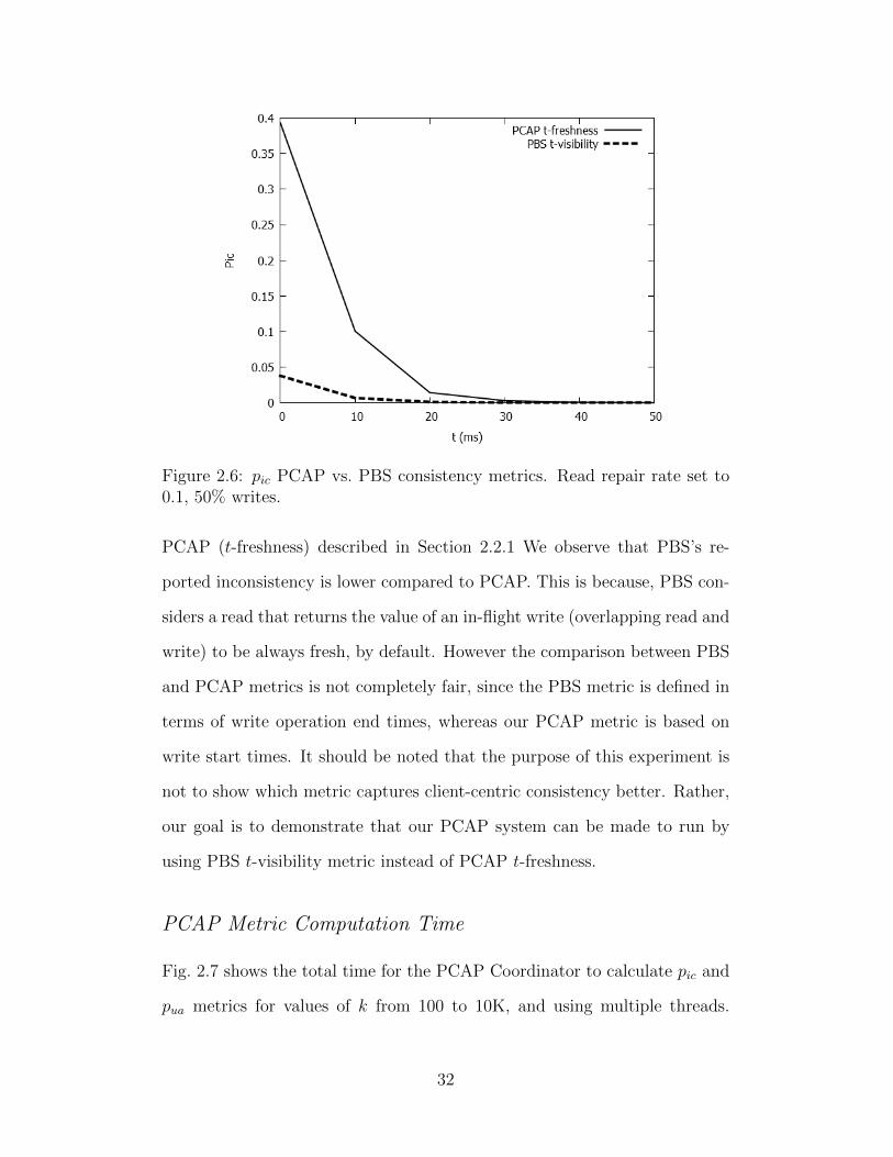
Figure 2.6: pic PCAP vs. PBS consistency metrics. Read repair rate set to0.1, 50% writes.

PCAP (t-freshness) described in Section 2.2.1 We observe that PBS’s re-

ported inconsistency is lower compared to PCAP. This is because, PBS con-

siders a read that returns the value of an in-flight write (overlapping read and

write) to be always fresh, by default. However the comparison between PBS

and PCAP metrics is not completely fair, since the PBS metric is defined in

terms of write operation end times, whereas our PCAP metric is based on

write start times. It should be noted that the purpose of this experiment is

not to show which metric captures client-centric consistency better. Rather,

our goal is to demonstrate that our PCAP system can be made to run by

using PBS t-visibility metric instead of PCAP t-freshness.

PCAP Metric Computation Time

Fig. 2.7 shows the total time for the PCAP Coordinator to calculate pic and

pua metrics for values of k from 100 to 10K, and using multiple threads.

32

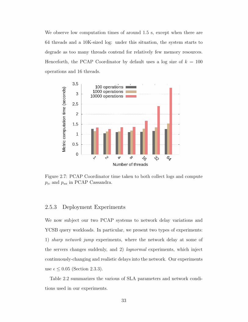
We observe low computation times of around 1.5 s, except when there are

64 threads and a 10K-sized log: under this situation, the system starts to

degrade as too many threads contend for relatively few memory resources.

Henceforth, the PCAP Coordinator by default uses a log size of k = 100

operations and 16 threads.

Figure 2.7: PCAP Coordinator time taken to both collect logs and computepic and pua in PCAP Cassandra.

2.5.3 Deployment Experiments

We now subject our two PCAP systems to network delay variations and

YCSB query workloads. In particular, we present two types of experiments:

1) sharp network jump experiments, where the network delay at some of

the servers changes suddenly, and 2) lognormal experiments, which inject

continuously-changing and realistic delays into the network. Our experiments

use ε ≤ 0.05 (Section 2.3.3).

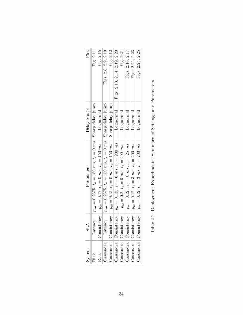
Table 2.2 summarizes the various of SLA parameters and network condi-

tions used in our experiments.

33

Syst

emS

LA

Par

amet

ers

Del

ayM

od

elP

lot

Ria

kL

aten

cypua

=0.

2375

,t a

=15

0ms,t c

=0ms

Sh

arp

del

ayju

mp

Fig

.2.

11

Ria

kC

on

sist

ency

pic

=0.

17,t c

=0ms,t a

=15

0ms

Log

nor

mal

Fig

.2.

15

Cass

and

raL

aten

cypua

=0.

2375

,t a

=15

0ms,t c

=0ms

Sh

arp

del

ayju

mp

Fig

s.2.

8,2.

9,2.

10

Cass

and

raC

on

sist

ency

pic

=0.

15,t c

=0ms,t a

=15

0ms

Sh

arp

del

ayju

mp

Fig

.2.

12

Cass

and

raC

on

sist

ency

pic

=0.

135,t c

=0ms,t a

=20

0ms

Log

nor

mal

Fig

s.2.

13,

2.14

,2.

19,

2.20

Cass

and

raC

on

sist

ency

pic

=0.

2,t c

=0ms,t a

=20

0ms

Log

nor

mal

Fig

.2.

21

Cass

and

raC

on

sist

ency

pic

=0.

125,t c

=0ms,t a

=25

ms

Log

nor

mal

Fig

s.2.

16,

2.17

Cass

and

raC

on

sist

ency

pic

=0.

12,t c

=3ms,t a

=20

0ms

Log

nor

mal

Fig

s.2.

22,

2.23

Cass

and

raC

on

sist

ency

pic

=0.

12,t c

=3ms,t a

=20

0ms

Log

nor

mal

Fig

s.2.

24,

2.25

Tab

le2.

2:D

eplo

ym

ent

Exp

erim

ents

:Sum

mar

yof

Set

tings

and

Par

amet

ers.

34

Latency SLA under Sharp Network Jump

Fig. 2.8 shows the timeline of a scenario for PCAP Cassandra using the

following latency SLA: pslaua = 0.2375, tc = 0 ms, ta = 150 ms.

In the initial segment of this run (t = 0 s to t = 800 s) the network delays

are small; the one-way server-to-LAN switch delay is 10 ms (this is half the

machine to machine delay, where a machine can be either a client or a server).

After the warm up phase, by t = 400 s, Fig. 2.8 shows that pua has converged

to the target SLA. Inconsistency pic stays close to zero.

We wish to measure how close the PCAP system is to the optimal-achievable

envelope (Section 2.2). The envelope captures the lowest possible values for

consistency (pic, tc), and latency (pua, ta), allowed by the network partition

model (α, tp) (Theorem 2). We do this by first calculating α for our specific

network, then calculating the optimal achievable non-SLA metric, and finally

seeing how close our non-SLA metric is to this optimal.

First, from Theorem 1 we know that the achievability region requires tc +

ta ≥ tp; hence, we set tp = tc + ta. Based on this, and the probability

distribution of delays in the network, we calculate analytically the exact

value of α as the fraction of client pairs whose propagation delay exceeds tp

(see Definition 5).

Given this value of α at time t, we can calculate the optimal value of pic

as pic(opt) = max(0, α − pua). Fig. 2.8 shows that in the initial part of the

plot (until t = 800 s), the value of α is close to 0, and the pic achieved by

PCAP Cassandra is close to optimal.

At time t = 800 s in Fig. 2.8, we sharply increase the one-way server-to-

LAN delay for 5 out of 9 servers from 10 ms to 26 ms. This sharp network

jump results in a lossier network, as shown by the value of α going up from

35

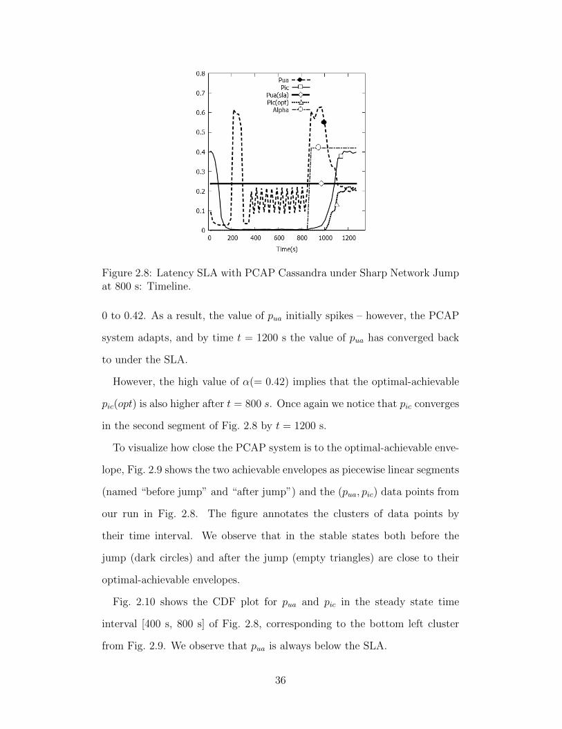
Figure 2.8: Latency SLA with PCAP Cassandra under Sharp Network Jumpat 800 s: Timeline.

0 to 0.42. As a result, the value of pua initially spikes – however, the PCAP

system adapts, and by time t = 1200 s the value of pua has converged back

to under the SLA.

However, the high value of α(= 0.42) implies that the optimal-achievable

pic(opt) is also higher after t = 800 s. Once again we notice that pic converges

in the second segment of Fig. 2.8 by t = 1200 s.

To visualize how close the PCAP system is to the optimal-achievable enve-

lope, Fig. 2.9 shows the two achievable envelopes as piecewise linear segments

(named “before jump” and “after jump”) and the (pua, pic) data points from

our run in Fig. 2.8. The figure annotates the clusters of data points by

their time interval. We observe that in the stable states both before the

jump (dark circles) and after the jump (empty triangles) are close to their

optimal-achievable envelopes.

Fig. 2.10 shows the CDF plot for pua and pic in the steady state time

interval [400 s, 800 s] of Fig. 2.8, corresponding to the bottom left cluster

from Fig. 2.9. We observe that pua is always below the SLA.

36

Figure 2.9: Latency SLA with PCAP Cassandra under Sharp Network Jump:Consistency-Latency Scatter plot.

Figure 2.10: Latency SLA with PCAP Cassandra under Sharp NetworkJump: Steady State CDF [400 s, 800 s].

37

Fig. 2.11 shows a scatter plot for our PCAP Riak system under a latency

SLA (pslaua = 0.2375, ta = 150 ms, tc = 0 ms). The sharp network jump

occurs at time t = 4300 s when we increase the one-way server-to-LAN delay

for 4 out of the 9 Riak nodes from 10 ms to 26 ms. It takes about 1200 s for

pua to converge to the SLA (at around t = 1400 s in the warm up segment

and t = 5500 s in the second segment).

Figure 2.11: Latency SLA with PCAP Riak under Sharp Network Jump:Consistency-Latency Scatter plot.

Consistency SLA under Sharp Network Jump

We present consistency SLA results for PCAP Cassandra (PCAP Riak results

are similar and are omitted). We use pslaic = 0.15, tc = 0 ms, ta = 150 ms.

The initial one-way server-to-LAN delay is 10 ms. At time 750 s, we increase

the one-way server-to-LAN delay for 5 out of 9 nodes to 14 ms. This changes

α from 0 to 0.42.

Fig. 2.12 shows the scatter plot. First, observe that the PCAP system

meets the consistency SLA requirements, both before and after the jump.

38

Figure 2.12: Consistency SLA with PCAP Cassandra under Sharp NetworkJump: Consistency-Latency Scatter plot.

Second, as network conditions worsen, the optimal-achievable envelope moves

significantly. Yet the PCAP system remains close to the optimal-achievable

envelope. The convergence time is about 100 s, both before and after the

jump.

Experiments with Realistic Delay Distributions

This section evaluates the behavior of PCAP Cassandra and PCAP Riak

under continuously-changing network conditions and a consistency SLA (la-

tency SLA experiments yielded similar results and are omitted).

Based on studies for enterprise data-centers [52] we use a lognormal distri-

bution for injecting packet delays into the network. We modified the Linux

traffic shaper to add lognormally distributed delays to each packet. Fig. 2.13

shows a timeline where initially (t = 0 to 800 s) the delays are lognor-

mally distributed, with the underlying normal distributions of µ = 3 ms

and σ = 0.3 ms. At t = 800 s we increase µ and σ to 4 ms and 0.4 ms

39

Figure 2.13: Consistency SLA with PCAP Cassandra under Lognormal delaydistribution: Timeline.

Figure 2.14: Consistency SLA with PCAP Cassandra under Lognormal delaydistribution: Consistency-Latency Scatter plot.

40

Figure 2.15: Consistency SLA with PCAP Riak under Lognormal delay dis-tribution: Timeline.

respectively. Finally at around 2100 s, µ and σ become 5 ms and 0.5 ms

respectively. Fig. 2.14 shows the corresponding scatter plot. We observe

that in all three time segments, the inconsistency metric pic: i) stays below

the SLA, and ii) upon a sudden network change converges back to the SLA.

Additionally, we observe that pua converges close to its optimal achievable

value.

Fig. 2.15 shows the effect of worsening network conditions on PCAP Riak.

At around t = 1300 s we increase µ from 1 ms to 4 ms, and σ from 0.1 ms

to 0.5 ms. The plot shows that it takes PCAP Riak an additional 1300 s to

have inconsistency pic converge to the SLA. Further the non-SLA metric pua

converges close to the optimal.

So far all of our experiments were conducted using lax timeliness require-

ments (ta = 150 ms, 200 ms), and were run on top of relatively high de-

lay networks. Next we perform a stringent consistency SLA experiment

(tc = 0 ms, pic = .125) with a very tight latency timeliness requirement

(ta = 25 ms). Packet delays are still lognormally distributed, but with lower

values. Fig. 2.16 shows a timeline where initially the delays are lognormally

41

distributed with µ = 1 ms, σ = 0.1 ms. At time t = 160 s we increase µ and

σ to 1.5 ms and 0.15 ms respectively. Then at time t = 320 s, we decrease

µ and σ to return to the initial network conditions. We observe that in all

three time segments, pic stays below the SLA, and quickly converges back

to the SLA after a network change. Since the network delays are very low

throughout the experiment, α is always 0. Thus the optimal pua is also 0.

We observe that pua converges very close to optimal before the first jump

and after the second jump (µ = 1 ms, σ = 0.1 ms). In the middle time

segment (t = 160 to 320 s), pua degrades in order to meet the consistency

SLA under slightly higher packet delays. Fig. 2.17 shows the corresponding

scatter plot. We observe that the system is close to the optimal envelope

in the first and last time segments, and the SLA is always met. We note

that we are far from optimal in the middle time segment, when the network

delays are slightly higher. This shows that when the network conditions are

relatively good, the PCAP system is close to the optimal envelope, but when

situations worsen we move away. The gap between the system performance

and the envelope indicates that the bound (Theorem 2) could be improved

further. We leave this as an open question.

Effect of Read Repair Rate Knob

All of our deployment experiments use read delay as the only control knob.

Fig. 2.18 shows a portion of a run when only read repair rate was used by our

PCAP Cassandra system. This was because read delay was already zero, and

we needed to push pic up to pslaic . First we notice that pua does not change

with read repair rate, as expected (Table 2.1). Second, we notice that the

convergence of pic is very slow – it changes from 0.25 to 0.3 over a long period

42

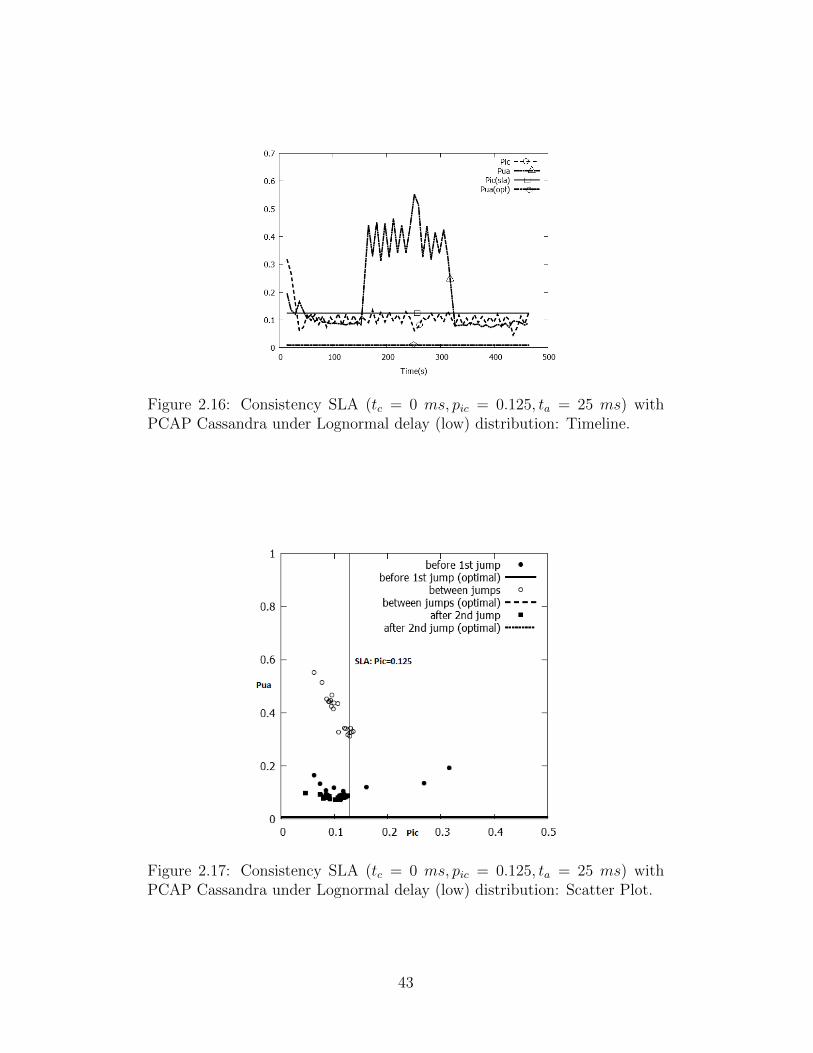
Figure 2.16: Consistency SLA (tc = 0 ms, pic = 0.125, ta = 25 ms) withPCAP Cassandra under Lognormal delay (low) distribution: Timeline.

Figure 2.17: Consistency SLA (tc = 0 ms, pic = 0.125, ta = 25 ms) withPCAP Cassandra under Lognormal delay (low) distribution: Scatter Plot.

43

Figure 2.18: Effect of Read Repair Rate on PCAP Cassandra. pic = 0.31,tc = 0 ms, ta = 100 ms.

of 1000 s.

Due to this slow convergence, we conclude that read repair rate is use-

ful only when network delays remain relatively stable. Under continuously

changing network conditions (e.g., a lognormal distribution) convergence may

be slower and thus read delay should be used as the only control knob.

Scalability

We measure scalability via an increased workload on PCAP Cassandra. Com-

pared to Fig. 2.14, in this new run we increased the number of servers from 9

to 32, and throughput to 16000 ops/s, and ensured that each server stores at

least some keys. All other settings are unchanged compared to Fig. 2.14. The

result is shown Fig. 2.19. Compared with Fig. 2.14, we observe an improve-

ment with scale – in particular, increasing the number of servers brings the

system closer to optimal. As the number of servers in the system increase, the

chance of finding a replica server close to a client proxy also increases. This

in turn lowers read latency, thus bringing the system closer to the optimal

envelope.

44

Figure 2.19: Scatter plot for same settings as Fig. 2.14, but with 32 serversand 16K ops/s.

Effect of Timeliness Requirement

The timeliness requirements in an SLA directly affect how close the PCAP

system is to the optimal-achievable envelope. Fig. 2.20 shows the effect

of varying the timeliness parameter ta in a consistency SLA (tc = 0 ms,

pic = 0.135) experiment for PCAP Cassandra with 10 ms node to LAN delays.

For each ta, we consider the cluster of the (pua, pic) points achieved by the

PCAP system in its stable state, calculate its centroid, and measure (and plot

on vertical axis) the distance d from this centroid to the optimal-achievable

consistency-latency envelope. Note that the optimal envelope calculation

also involves ta, since α depends on it (Section 2.5.3).

Fig. 2.20 shows that when ta is too stringent (< 100 ms), the PCAP system

may be far from the optimal envelope even when it satisfies the SLA. In the

case of Fig. 2.20, this is because in our network, the average time to cross four

hops (client to coordinator to replica, and the reverse) is 20×4 = 80 ms.8 As

8Round-trip time for each hop is 2× 10 = 20 ms.

45

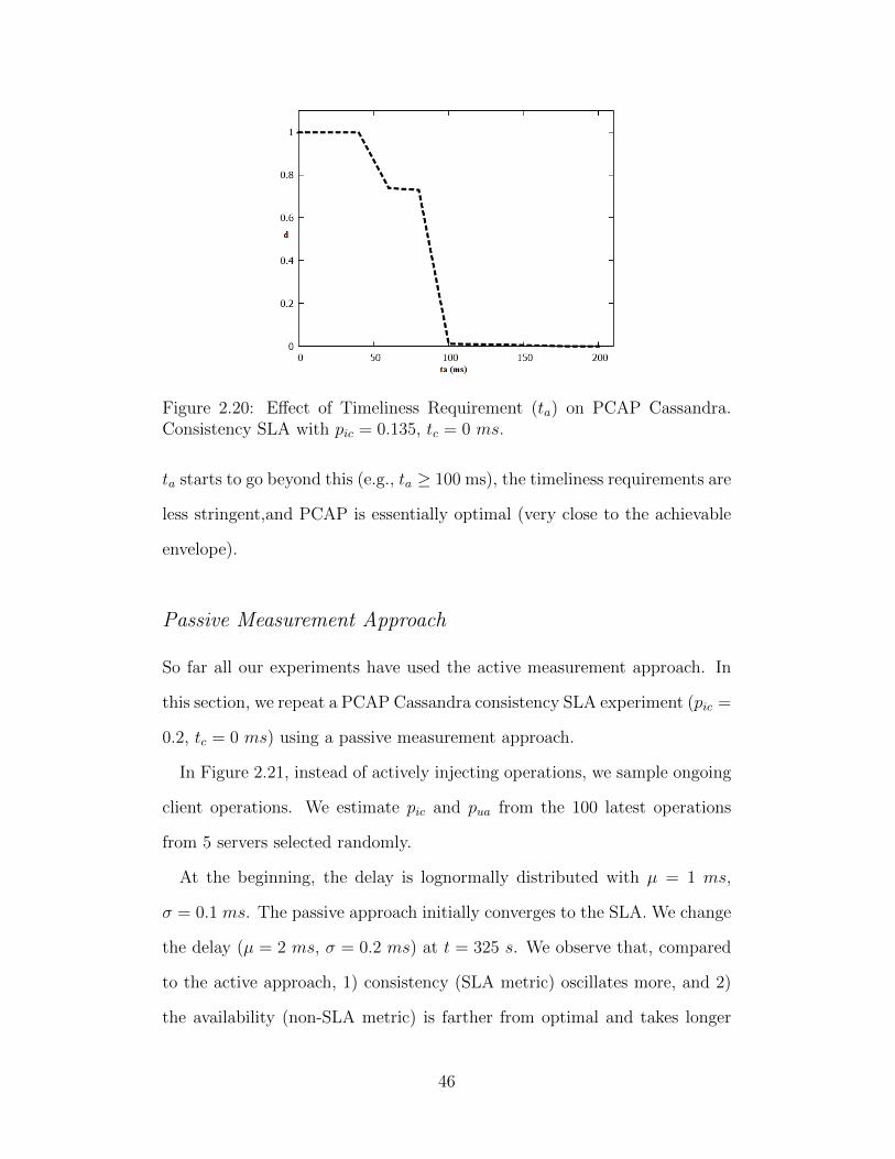
Figure 2.20: Effect of Timeliness Requirement (ta) on PCAP Cassandra.Consistency SLA with pic = 0.135, tc = 0 ms.

ta starts to go beyond this (e.g., ta ≥ 100 ms), the timeliness requirements are

less stringent,and PCAP is essentially optimal (very close to the achievable

envelope).

Passive Measurement Approach

So far all our experiments have used the active measurement approach. In

this section, we repeat a PCAP Cassandra consistency SLA experiment (pic =

0.2, tc = 0 ms) using a passive measurement approach.

In Figure 2.21, instead of actively injecting operations, we sample ongoing

client operations. We estimate pic and pua from the 100 latest operations

from 5 servers selected randomly.

At the beginning, the delay is lognormally distributed with µ = 1 ms,

σ = 0.1 ms. The passive approach initially converges to the SLA. We change

the delay (µ = 2 ms, σ = 0.2 ms) at t = 325 s. We observe that, compared

to the active approach, 1) consistency (SLA metric) oscillates more, and 2)

the availability (non-SLA metric) is farther from optimal and takes longer

46

Figure 2.21: Consistency SLA with PCAP Cassandra under Lognormal delaydistribution: Timeline (Passive).

to converge. For the passive approach, SLA convergence and non-SLA opti-

mization depends heavily on the sampling of operations used to estimate the

metrics. Thus we conclude that it is harder to satisfy SLA and optimize the

non-SLA metric with the passive approach.

YCSB Benchmark Experiments

So far we have used YCSB client workloads for all our experiments. Specifi-

cally, we used a read-heavy (80% reads) workload. However a 80% read-heavy

workload is not one of the standard YCSB benchmark workloads [37]. Thus

to facilitate benchmark comparisons of PCAP with other systems with sim-

ilar capabilities in the future, we show experimental results for PCAP using

two standard YCSB benchmark workloads: (1) Workload A (Update heavy)

which has 50/50 reads and writes, and (2) Workload D (Read latest with

95% reads) where most recently inserted records are the most popular.

Read Latest Workload In this section, we show the results of a PCAP

Cassandra consistency SLA experiment (pic = 0.12, tc = 3 ms, ta = 200 ms)

47

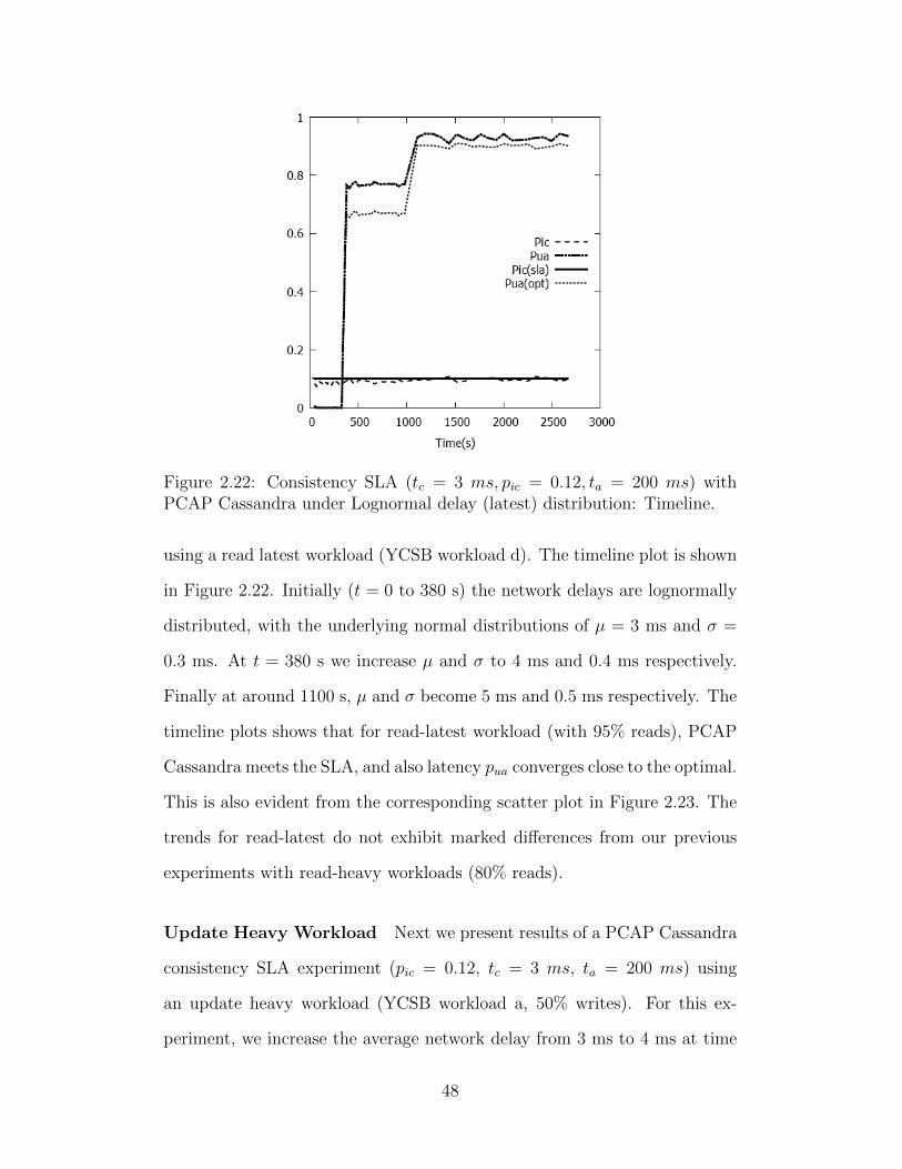
Figure 2.22: Consistency SLA (tc = 3 ms, pic = 0.12, ta = 200 ms) withPCAP Cassandra under Lognormal delay (latest) distribution: Timeline.

using a read latest workload (YCSB workload d). The timeline plot is shown

in Figure 2.22. Initially (t = 0 to 380 s) the network delays are lognormally

distributed, with the underlying normal distributions of µ = 3 ms and σ =

0.3 ms. At t = 380 s we increase µ and σ to 4 ms and 0.4 ms respectively.

Finally at around 1100 s, µ and σ become 5 ms and 0.5 ms respectively. The

timeline plots shows that for read-latest workload (with 95% reads), PCAP

Cassandra meets the SLA, and also latency pua converges close to the optimal.

This is also evident from the corresponding scatter plot in Figure 2.23. The

trends for read-latest do not exhibit marked differences from our previous

experiments with read-heavy workloads (80% reads).

Update Heavy Workload Next we present results of a PCAP Cassandra

consistency SLA experiment (pic = 0.12, tc = 3 ms, ta = 200 ms) using

an update heavy workload (YCSB workload a, 50% writes). For this ex-

periment, we increase the average network delay from 3 ms to 4 ms at time

48

Figure 2.23: Consistency SLA (tc = 3 ms, pic = 0.12, ta = 200 ms) withPCAP Cassandra under Lognormal delay (latest) distribution: Scatter Plot.

540 s, and from 4 ms to 5 ms at time 1630 s. The timeline plot in Figure 2.24

indicates poor convergence behavior compared to read-heavy and read-latest

distributions. Especially after the second jump, it takes about 1000 s to con-

verge back to SLA. This is because our target key-value stores (Cassandra,

Riak) rely heavily on read-repair mechanisms to sycnhronize replicas in the

background. With an update-heavy workload, read-repair synchronization

mechanisms lose their effectiveness, which makes it harder to guarantee con-

sistency SLA convergence. The scatter plot in Figure 2.25 however shows

that PCAP Cassandra performs close to the optimal envelope, except for

some outliers which are transient states before convergence. It should be

noted that an update-heavy workload is not a realistic workload for many

key-value stores, and we have only presented results with such workloads

for future comparison with other systems using standard benchmarks like

YCSB.

49

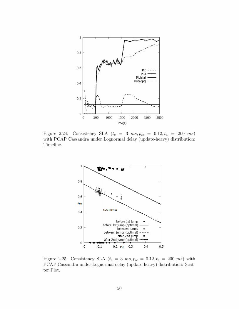
Figure 2.24: Consistency SLA (tc = 3 ms, pic = 0.12, ta = 200 ms)with PCAP Cassandra under Lognormal delay (update-heavy) distribution:Timeline.

Figure 2.25: Consistency SLA (tc = 3 ms, pic = 0.12, ta = 200 ms) withPCAP Cassandra under Lognormal delay (update-heavy) distribution: Scat-ter Plot.

50

2.6 Related Work

In this section we discuss related work for our PCAP system.

2.6.1 Consistency-Latency Tradeoffs

In addition to the Weak CAP Principle [76] and PACELC [40] discussed in

Section 2.1, there has been work on theoretically characterizing the trade-

off between latency and strong consistency models. Attiya and Welch [47]

studied the tradeoff between latency and linearizability and sequential con-

sistency. Subsequent work has explored linearizablity under different delay

models [72, 112]. All these papers are concerned with strong consistency

models whereas we consider t-freshness, which models data freshness in even-

tually consistent systems. Moreover, their delay models are different from

our partition model. There has been theoretical work on probabilistic quo-

rum systems [41, 101, 111]. Their consistency models are different from ours;

moreover, they did not consider the tradeoff between consistency and avail-

ability.

There are two classes of systems that are closest to our work. The first

class of systems are concerned with metrics for measuring data freshness

or staleness. We do not compare our work against this class of systems

in this chapter, as it is not our goal to propose yet another consistency

model or metric. [49, 50] propose a probabilistic consistency model (PBS) for

quorum-based stores, but did not consider latency, soft partitions or the CAP

theorem. [81] propose a time-based staleness metric called ∆-atomicity. ∆-

atomicity is considered the gold standard for measuring atomicity violations

(staleness) across multiple read and write operations. The Γ metric [82]

is inspired by the ∆ metric and improves upon it on multiple fronts. For

51

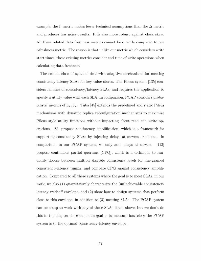
example, the Γ metric makes fewer technical assumptions than the ∆ metric

and produces less noisy results. It is also more robust against clock skew.

All these related data freshness metrics cannot be directly compared to our

t-freshness metric. The reason is that unlike our metric which considers write

start times, these existing metrics consider end time of write operations when

calculating data freshness.

The second class of systems deal with adaptive mechanisms for meeting

consistency-latency SLAs for key-value stores. The Pileus system [135] con-

siders families of consistency/latency SLAs, and requires the application to

specify a utility value with each SLA. In comparison, PCAP considers proba-

bilistic metrics of pic, pua. Tuba [45] extends the predefined and static Pileus

mechanisms with dynamic replica reconfiguration mechanisms to maximize

Pileus style utility functions without impacting client read and write op-

erations. [83] propose consistency amplification, which is a framework for

supporting consistency SLAs by injecting delays at servers or clients. In

comparison, in our PCAP system, we only add delays at servers. [113]

propose continuous partial quorums (CPQ), which is a technique to ran-

domly choose between multiple discrete consistency levels for fine-grained

consistency-latency tuning, and compare CPQ against consistency amplifi-

cation. Compared to all these systems where the goal is to meet SLAs, in our

work, we also (1) quantitatively characterize the (un)achievable consistency-

latency tradeoff envelope, and (2) show how to design systems that perform

close to this envelope, in addition to (3) meeting SLAs. The PCAP system

can be setup to work with any of these SLAs listed above; but we don’t do

this in the chapter since our main goal is to measure how close the PCAP

system is to the optimal consistency-latency envelope.

52

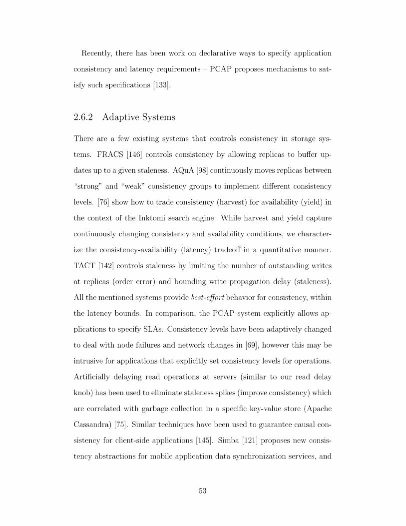
Recently, there has been work on declarative ways to specify application

consistency and latency requirements – PCAP proposes mechanisms to sat-

isfy such specifications [133].

2.6.2 Adaptive Systems

There are a few existing systems that controls consistency in storage sys-

tems. FRACS [146] controls consistency by allowing replicas to buffer up-

dates up to a given staleness. AQuA [98] continuously moves replicas between

“strong” and “weak” consistency groups to implement different consistency

levels. [76] show how to trade consistency (harvest) for availability (yield) in

the context of the Inktomi search engine. While harvest and yield capture

continuously changing consistency and availability conditions, we character-

ize the consistency-availability (latency) tradeoff in a quantitative manner.

TACT [142] controls staleness by limiting the number of outstanding writes

at replicas (order error) and bounding write propagation delay (staleness).

All the mentioned systems provide best-effort behavior for consistency, within

the latency bounds. In comparison, the PCAP system explicitly allows ap-

plications to specify SLAs. Consistency levels have been adaptively changed

to deal with node failures and network changes in [69], however this may be

intrusive for applications that explicitly set consistency levels for operations.

Artificially delaying read operations at servers (similar to our read delay

knob) has been used to eliminate staleness spikes (improve consistency) which

are correlated with garbage collection in a specific key-value store (Apache

Cassandra) [75]. Similar techniques have been used to guarantee causal con-

sistency for client-side applications [145]. Simba [121] proposes new consis-

tency abstractions for mobile application data synchronization services, and

53

allows applications to choose among various consistency models.

For stream processing, [77] propose a control algorithm to compute the

optimal resource requirements to meet throughput requirements. There has

been work on adaptive elasticity control for storage [104], and adaptively

tuning Hadoop clusters to meet SLAs [89]. Compared to the controllers

present in these systems, our PCAP controller achieves control objectives [87]

using a different set of techniques to meet SLAs for key-value stores.

2.7 Summary

In this chapter, we have first formulated and proved a probabilistic variation

of the CAP theorem which took into account probabilistic models for consis-

tency, latency, and soft partitions within a data-center. Our theorems show

the un-achievable envelope, i.e., which combinations of these three models

make them impossible to achieve together. We then show how to design

systems (called PCAP) that (1) perform close to this optimal envelope, and

(2) can meet consistency and latency SLAs derived from the corresponding

models. We then incorporated these SLAs into Apache Cassandra and Riak

running in a single data-center. Our experiments with YCSB workloads and

realistic traffic demonstrated that our PCAP system meets the SLAs, that

its performance is close to the optimal-achievable consistency-availability en-

velope, and that it scales well.

54

Chapter 3

GeoPCAP: Probabilistic Composition andAdaptive Control for Geo-distributed

Key-Value Stores

In this chapter, we extend our PCAP system presented in Chapter 2 from a

single data-center to multiple geo-distributed data-centers. We call this sys-

tem GeoPCAP. The key contribution of GeoPCAP is a set of rules for com-

posing probabilistic consistency/latency models from across multiple data-

centers in order to derive the global consistency-latency tradeoff behavior.

Realistic simulations demonstrate that GeoPCAP can satisfactorily meet

consistency/latency SLAs for applications interacting with multiple data-

centers, while optimizing the other metric.

3.1 Introduction

Distributed key-value stores (e.g., Cassandra [8], Riak [7], Dynamo [71],

Voldemort [24]) are preferred by applications for whom eventual consis-

tency suffices, but where high availability (i.e., fast reads and writes [40])

is paramount. Availability is a critical metric for such cloud services because

latency is correlated to user satisfaction – for instance, a 500 ms increase in

latency for operations at Google.com can cause a 20% drop in revenue [1]. At

Amazon, this translates to a $6M yearly loss per added millisecond of latency

[2]. At the same time, clients in such applications expect freshness, i.e., data

returned by a read to a key should come from the latest writes done to that

key by any client. For instance, Netflix uses Cassandra to track positions in

55

each video [66], and freshness of data translates to accurate tracking and

user satisfaction. This implies a time-based notion of consistency.

Internet Web applications built out of key value stores are facing an ever

worsening scalability challenge due to multiple reasons. First, the number of

users is growing across an increasing number of geographic regions (Facebook

had over 1.39 billion active users as of Dec 2014 [14]). Second, the storage

needs per user is also growing as more information is stored online. As users

accumulate more data, the systems also store more information per user

for generating targeted ads and user recommendations. Finally, replication

of data for fault-tolerance also rapidly increases storage space. As a result

many of these applications need to be geo-distributed, hence the need for

geo-distributed deployment for key-value stores.

Geo-distributed key-value stores use geo-replication, meaning the same

key is replicated at different data-centers. So these systems offer high avail-

ability by replicating data across datacenters, and low latency by placing

data close to clients. From a client perspective, there should be no difference

between interacting with a single datacenter vs interacting with multiple geo-

distributed datacenters transparently. Hence if we compose a geo-distributed

key-value service by composing multiple instances of a key-value service (one

in each data-center), then the customer should be transparent to this geo-

distribution.

For example, assume an Internet service has three storage systems at

three regional data-centers; one in America, one in Europe, and one in

Asia. Depending on user requirements, the data for a particular user can

be stored/replicated from one to all three locations. Also the storage sys-

tems within each region can replicate the data multiple times. Based on

storage configurations, each data-center storage system instance offers differ-

56

ent tradeoffs between data consistency and latency/availability. Thus when

the service provider offers a read API to a client, it should transparently

compose the service offered from one or more per data-center instances in

order to satisfy the client read request with a given consistency or latency

requirement. This requires a principled way to compose consistency-latency

guarantees from different geo-distributed storage services.

In this chapter we develop a formal probabilistic framework for composing

consistency-latency models of different storage services geo-distributed across

multiple data-centers. A service provider can thus use these rules to com-

pose services of different storage instances to meet desired consistency-latency

tradeoffs. We offer two types of composition rules. First the QUICKEST com-

position rule ensures that at-least one data-center instance provides the de-

sired service level. The other rule is ALL composition, which guarantees all

data-centers meet the desired per data-center consistency-latency require-

ment. Our rules are generic and hold for an arbitrary number of data-center

instances.

Next we present the design and implementation of a system called GeoP-

CAP, which is a geo-distributed extension of the PCAP system presented in

Chapter 2. GeoPCAP uses the probabilistic composition rules and an adap-

tive control loop based on PID control theory to continuously meet SLAs for

a geo-distributed key-value storage system under WAN network delay varia-

tions. Realistic simulation results indicate that GeoPCAP can satisfactorily

meet SLAs in the presence of WAN delay variations.

57

3.2 System Model

Assume there are n data-centers. Each data-center stores multiple replicas

for each data-item. When a client application submits a query, the query

is first forwarded to the data-center closest to the client. We call this data-

center the local data-center for the client. If the local data-center stores a

replica of the queried data item, that replica might not have the latest value,

since write operations at other data-centers could have updated the data

item. Thus in our system model, the local data-center contacts one or more

of other remote data-centers, to retrieve (possibly) fresher values for the data

item.

3.3 Probabilistic Composition Rules

Each data-center is running our PCAP-enabled key-value store. Each such

PCAP instance defines per data-center probabilistic latency and consistency

models (Section 2.2). To obtain the global behavior, we need to compose

these probabilistic consistency and latency/availability models across differ-

ent data-centers. This is done by our composition rules.

The composition rules for merging independent latency/consistency mod-

els from data-centers check whether the SLAs are met by the composed sys-

tem. Since single data-center PCAP systems define probabilistic latency and

consistency models, our composition rules are also probabilistic in nature.

However in reality, our composition rules do not require all data-centers to

run PCAP-enabled key-value stores systems. As long as we can measure con-

sistency and latency at each data-center, we can estimate the probabilistic

models of consistency/latency at each data-center and use our composition

rules to merge them.

58

We consider two types of composition rules: (1) QUICKEST (Q), where at-

least one data-center (e.g., the local or closest remote data-center) satisfies

client specified latency or freshness (consistency) guarantees; and (2) ALL (A),

where all the data-centers must satisfy latency or freshness guarantees. These

two are, respectively, generalizations of Apache Cassandra multi-data-center

deployment [38] consistency levels (CL): LOCAL QUORUM and EACH QUORUM.

Compared to Section 2.2, which analyzed the fraction of executions that

satisfy a predicate (the proportional approach), in this section we use a sim-

pler probabilistic approach. This is because although the proportional ap-

proach is more accurate, it is more intractable than the probabilistic model

in the geo-distributed case.

Our probabilistic composition rules fall into three categories: (1) compos-

ing consistency models; (2) composing latency models; and (3) composing a

wide-area-network (WAN) partition model with a data-center (consistency

or latency) model. The rules are summarized in Table 3.1, and we discuss

them next.

3.3.1 Composing Latency Models

Assume there are n data-centers storing the replica of a key with latency

models (t1a, p1ua), (t

2a, p

2ua), . . . , (t

na , p

nua). Let CA denote the composed system.

Let (pcua, tca) denote the latency model of the composed system CA. This

indicates that the fraction of reads in CA that complete within tca time units

is at least (1− pcua). This is the latency SLA expected by clients. Let pcua(t)

denote the probability of missing deadline by t time units in the composed

model. Let Xj denote the random variable measuring read latency in data

center j. Let Ej(t) denote the event that Xj > t. By definition we have that,

59

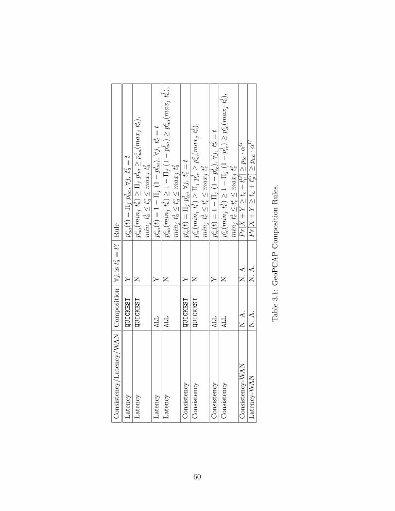
Con

sist

ency

/L

aten

cy/W

AN

Com

pos

itio

n∀j,i

stj a

=t?

Ru

le

Late

ncy

QUICKEST

Ypc ua(t

)=

Πjpj ua,∀j,tj a

=t

Late

ncy

QUICKEST

Npc ua(min

jtj a

)≥

Πjpj ua≥pc ua(maxjtj a

),

min

jtj a≤tc a≤maxjtj a

Late

ncy

ALL

Ypc ua(t

)=

1−

Πj

(1−pj ua),∀j,tj a

=t

Late

ncy

ALL

Npc ua(min

jtj a

)≥

1−

Πj

(1−pj ua)≥pc ua(maxjtj a

),

min

jtj a≤tc a≤maxjtj a

Con

sist

ency

QUICKEST

Ypc ic

(t)

=Π

jpj ic

,∀j,tj c

=t

Con

sist

ency

QUICKEST

Npc ic

(min

jtj c

)≥

Πjpj ic≥pc ic

(maxjtj c

),

min

jtj c≤tc c≤maxjtj c

Con

sist

ency

ALL

Ypc ic

(t)

=1−

Πj

(1−pj ic

),∀j,tj c

=t

Con

sist

ency

ALL

Npc ic

(min

jtj c

)≥

1−

Πj

(1−pj ic

)≥pc ic

(maxjtj c

),

min

jtj c≤tc c≤maxjtj c

Con

sist

ency

-WA

NN

.A

.N

.A

.Pr[X

+Y≥t c

+tG p

]≥pic·α

G

Late

ncy

-WA

NN

.A

.N

.A

.Pr[X

+Y≥t a

+tG p

]≥pua·α

G

Tab

le3.

1:G

eoP

CA

PC

omp

osit

ion

Rule

s.

60

Pr[Ej(tja)] = pjua, and Pr[Ej(t

ja)] = 1− pjua. Let fj(t) denote the cumulative

distribution function (CDF) for Xj. So by definition, fj(tja) = Pr[Xj ≤ tja] =

1− Pr[Xj > tja]. The following theorem articulates the probabilistic latency

composition rules:

Theorem 3 Let n data-centers store the replica for a key with latency mod-

els (t1a, p1ua), (t

2a, p

2ua), . . . , (t

na , p

nua). Let CA denote the composed system with

latency model (pcua, tca). Then for composition rule QUICKEST we have:

pcua(minj tja) ≥ Πj p

jua ≥ pcua(maxj t

ja), (3.1)

and minj tja ≤ tca ≤ maxj t

ja,

wherej ∈ {1, · · · , n}.

For composition rule ALL,

pcua(minj tja) ≥ 1− Πj (1− pjua) ≥ pcua(maxj t

ja), (3.2)

and minj tja ≤ tca ≤ maxj t

ja,

wherej ∈ {1, · · · , n}.

Proof: We outline the proof for composition rule QUICKEST. In QUICKEST,

a latency deadline t is violated in the composed model when all data-centers

miss the t deadline. This happens with probability pcua(t) (by definition). We

first prove a simpler Case 1, then the general version in Case 2.

Case 1: Consider the simple case where all tja values are identical, i.e.,

∀j, tja = ta: pcua(ta) = Pr[∩iEi(ta)] = ∩iPr[Ei(ta)] = Πip

iua (assuming inde-

pendence across data-centers).

61

Case 2:

Let,

tia = minj tja (3.3)

Then,

∀j, tja ≥ tia (3.4)

Then, by definition of CDF function,

∀j, fj(tia) ≤ fj(tja) (3.5)

By definition,

∀j, (Pr[Xj ≤ tia] ≤ Pr[Xj ≤ tja]) (3.6)

∀j, (Pr[Xj > tia] ≥ Pr[Xj > tja]) (3.7)

Multiplying all,

Πj Pr[Xj > tia] ≥ Πj Pr[Xj > tja] (3.8)

But this means,

pcua(tia) ≥ Πj p

jua (3.9)

pcua(minj tja) ≥ Πj p

jua (3.10)

62

Similarly, let

tka = maxj tja (3.11)

Then,

∀j, tka ≥ tja (3.12)

∀j, (Pr[Xj > tja] ≥ Pr[Xj > tka]) (3.13)

Πj Pr[Xj > tja] ≥ Πj Pr[Xj > tka] (3.14)

Πj pjua ≥ pcua(t

ka) (3.15)

Πj pjua ≥ pcua(maxj t

ja) (3.16)

Finally combining Equations 3.10, and 3.16, we get Equation 3.1.

The proof for composition rule ALL follows similarly. In this case, a latency

deadline t is satisfied when all data-centers satisfy the deadline. So a dead-

line miss in the composed model means at-least one data-center misses the

deadline. The derivation of the composition rules are similar and we invite

the reader to work them out to arrive at the equations depicted in Table 3.1.

2

63

Figure 3.1: Symmetry of freshness and latency requirements.

3.3.2 Composing Consistency Models

t-latency (Definition 3) and t-freshness (Definitions 1) guarantees are time-

symmetric (Figure 3.1). While t-lateness can be considered a deadline in the

future, t-freshness can be considered a deadline in the past. This means that

for a given read, t-freshness constrains how old a read value can be. So the

composition rules remain the same for consistency and availability.

Thus the consistency composition rules can be obtained by substituting

pua with pic and ta with tc in the latency composition rules (last 4 rows in

Table 3.1).

This leads to the following theorem for consistency composition:

Theorem 4 Let n data-centers store the replica for a key with consistency

models (t1c , p1ic), (t

2c , p

2ic), . . . , (t

nc , p

nic). Let CA denote the composed system with

consistency model (pcic, tcc). Then for composition rule QUICKEST we have:

pcic(minj tjc) ≥ Πj p

jic ≥ pcic(maxj t

jc), (3.17)

and minj tjc ≤ tcc ≤ maxj t

jc,

wherej ∈ {1, · · · , n}.

For composition rule ALL,

64

pcic(minj tjc) ≥ 1− Πj (1− pjic) ≥ pcic(maxj t

jc), (3.18)

and minj tjc ≤ tcc ≤ maxj t

jc,

wherej ∈ {1, · · · , n}.

3.3.3 Composing Consistency/Latency Model with a WANPartition Model

All data-centers are connected to each other through a wide-area-network

(WAN). We assume the WAN follows a partition model (tGp , αG). This indi-

cates that αG fraction of messages passing through the WAN suffers a delay

> tGp . Note that the WAN partition model is distinct from the per data-

center partition model (Definition 5). Let X denote the latency in a remote

data-center, and Y denote the WAN latency of a link connecting the local

data-center to this remote data-center (with latency X). Then the total

latency of the path to the remote data-center is X + Y .1

Pr[X + Y ≥ ta + tGp ] ≥ (Pr[X ≥ ta] · Pr[Y ≥ tGp ]) = pua · αG. (3.19)

Here we assume the WAN latency, and data-center latency distributions are

independent. Note that Equation 3.19 gives a lower bound of the probability.

In practice we can estimate the probability by sampling both X and Y , and

estimating the number of times (X + Y ) exceeds (ta + tGp ).

1We ignore the latency of the local data-center in this rule, since the local data-centerlatency is used in the latency composition rule (Section 3.3.1).

65

Figure 3.2: Example of composition rules in action.

3.3.4 Example

The example in Figure 3.2 shows the composition rules in action. In this

example, there is one local data-center and 2 replica data-centers. Each

data-center can hold multiple replicas of a data-item. First we compose each

replica data-center latency model with the WAN partition model. Second we

take the WAN-latency composed models for each data-center and compose

them using the QUICKEST rule (Table 3.1, bottom part).

3.4 GeoPCAP Control Knob

We use a similar delay knob to meet the SLAs in a geo-distributed setting.

We call this the geo-delay knob and denote it as ∆. The time delay ∆ is the

delay added at the local data-center to a read request received from a client

before it is forwarded to the replica data-centers. ∆ affects the consistency-

66

latency trade-off in a manner similar to the read delay knob in a data-center

(Section 2.3.1). Increasing the knob tightens the deadline at each replica

data-center, thus increasing per data-center latency (pua). Similar to read

delay (Figure 2.1), increasing the geo delay knob improves consistency, since

it gives each data-center time to commit latest writes.

3.5 GeoPCAP Control Loop

Our GeoPCAP system uses a control loop depicted in Figure 3.3 for the

Consistency SLA case using the QUICKEST composition rule. The control

loops for the other three combinations (Consistency-QUICKEST, Latency-ALL,

Latency-QUICKEST) are similar.

Initially, we opted to use the single data-center multiplicative control loop

(Section 2.3.3) for GeoPCAP. However, the multiplicative approach led to

increased oscillations for the composed consistency (pic) and latency (pua)

metrics in a geo-distributed setting. The multiplicative approach sufficed for

the single data-center PCAP system, since the oscillations were bounded in

steady-state. However, the increased oscillations in a geo-distributed setting

prompted us to use a control theoretic approach for GeoCAP.

As a result, we use a PID control theory approach [46] for the GeoPCAP

controller. The controller runs an infinite loop, so that it can react to network

delay changes and meet SLAs. There is a tunable sleep time at the end of

each iteration (1 sec in Section 3.6 simulations). Initially the geo-delay ∆ is

set to zero. At each iteration of the loop, we use the composition rules to

estimate pcic(t), where t = tslac + tGp − ∆. We also keep track of composed

pcua() values. We then compute the error, as the difference between current

composed pic and the SLA. Finally the geo-delay change is computed using

67

1: procedure control(SLA =< pslaic , tslac , tslaa >)

2: Geo-delay ∆ := 03: E := 0, Errorold := 04: set kp, kd, ki for PID control (tuning)5: Let (tGp , α

G) be the WAN partition model6: while (true) do7: for each data-center i do8: Let Fi denote the random freshness interval at i9: Let Li denote the random operation latency at i

10: Let Wi denote the WAN latency of the link to i11: Estimate piic := Pr[Fi + Wi > tslac + tGp + ∆] // WAN compo-

sition (Section 3.3.3)12: Estimate piua := Pr[Li +Wi > ta + tGp −∆ = tslaa ]13: end for14: pcic := Πip

iic, p

cua := Πip

iua // Consistency/Latency composition

(Sections 3.3.1 3.3.2)15: Error := pcic − pslaic

16: dE := Error − Errorold17: E := E + Error18: u := kp · Error + kd · dE + ki · E19: ∆ := ∆ + u;20: end while21: end procedure

Figure 3.3: Adaptive Control Loop for GeoPCAP Consistency SLA(QUICKEST Composition).

68

the PID control law [46] as follows:

u = kp · Error(t) + kd ·dError(t)

dt+ ki ·

∫Error(t)dt (3.20)

Here, kp, kd, ki represent the proportional, differential, and integral gain

factors for the PID controller respectively. There is a vast amount of litera-

ture on tuning these gain factors for different control systems [46]. Later in

our experiments, we discuss how we set these factors to get SLA convergence.

Finally at the end of the iteration, we increase ∆ by u. Note that u could

be negative, if the metric is less than the SLA.

Note that for the single data-center PCAP system, we used a multiplicative

control loop (Section 2.3.3), which outperformed the unit step size policy.

For GeoPCAP, we employ a PID control approach. PID is preferable to the

multiplicative approach, since it guarantees fast convergence, and can reduce

oscillation to arbitrarily small amounts. However PID’s stability depends

on proper tuning of the gain factors, which can result in high management

overhead. On the other hand the multiplicative control loop has a single

tuning factor (the multiplicative factor), so it is easier to manage. Later in

Section 3.6 we experimentally compare the PID and multiplicative control

approaches.

3.6 GeoPCAP Evaluation

We evaluate GeoPCAP with a Monte-Carlo simulation. In our setup, we have

four data-centers, among which three are remote data-centers holding repli-

cas of a key, and the fourth one is the local data-center. At each iteration,

we estimate t-freshness per data-center using a variation of the well-known

WARS model [50]. The WARS model is based on Dynamo style quorum

69

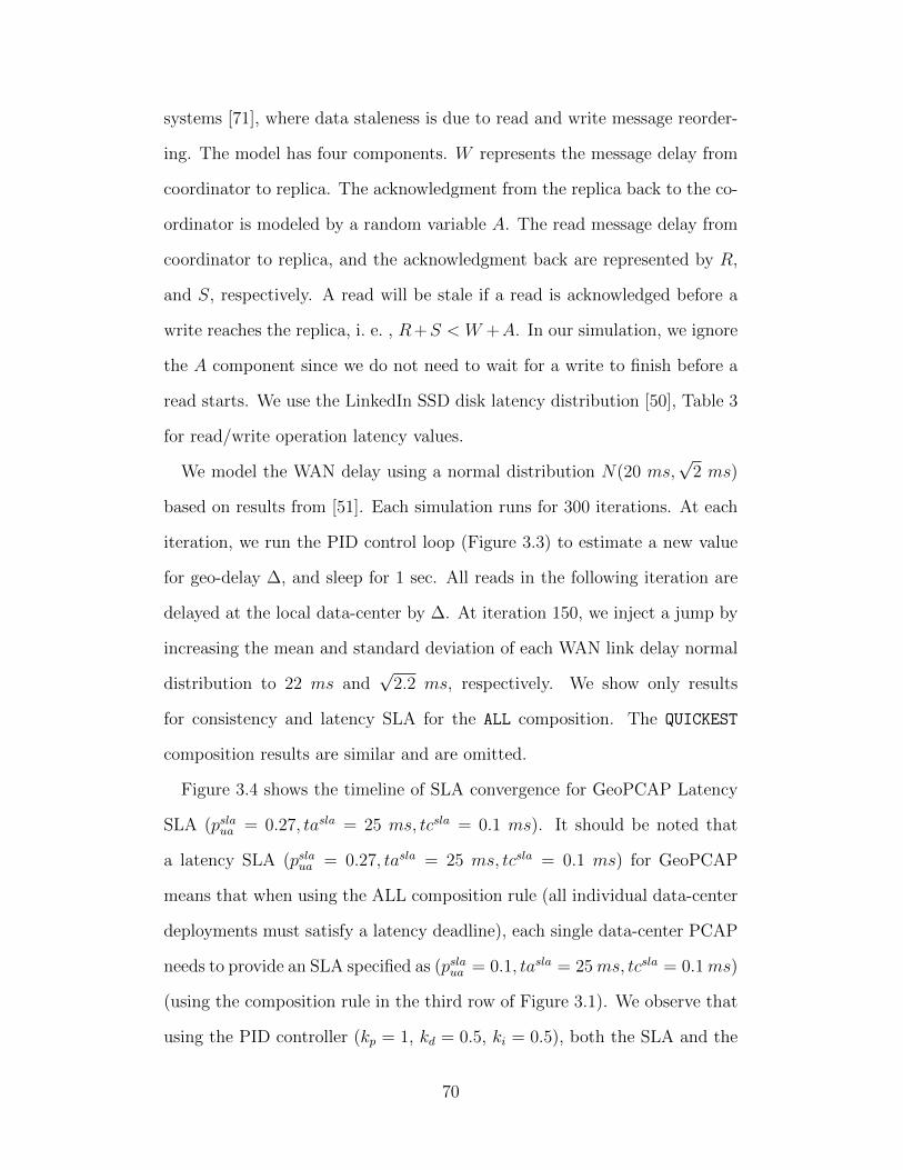
systems [71], where data staleness is due to read and write message reorder-

ing. The model has four components. W represents the message delay from

coordinator to replica. The acknowledgment from the replica back to the co-

ordinator is modeled by a random variable A. The read message delay from

coordinator to replica, and the acknowledgment back are represented by R,

and S, respectively. A read will be stale if a read is acknowledged before a

write reaches the replica, i. e. , R+S < W +A. In our simulation, we ignore

the A component since we do not need to wait for a write to finish before a

read starts. We use the LinkedIn SSD disk latency distribution [50], Table 3

for read/write operation latency values.

We model the WAN delay using a normal distribution N(20 ms,√

2 ms)

based on results from [51]. Each simulation runs for 300 iterations. At each

iteration, we run the PID control loop (Figure 3.3) to estimate a new value

for geo-delay ∆, and sleep for 1 sec. All reads in the following iteration are

delayed at the local data-center by ∆. At iteration 150, we inject a jump by

increasing the mean and standard deviation of each WAN link delay normal

distribution to 22 ms and√

2.2 ms, respectively. We show only results

for consistency and latency SLA for the ALL composition. The QUICKEST

composition results are similar and are omitted.

Figure 3.4 shows the timeline of SLA convergence for GeoPCAP Latency

SLA (pslaua = 0.27, tasla = 25 ms, tcsla = 0.1 ms). It should be noted that

a latency SLA (pslaua = 0.27, tasla = 25 ms, tcsla = 0.1 ms) for GeoPCAP

means that when using the ALL composition rule (all individual data-center

deployments must satisfy a latency deadline), each single data-center PCAP

needs to provide an SLA specified as (pslaua = 0.1, tasla = 25ms, tcsla = 0.1ms)

(using the composition rule in the third row of Figure 3.1). We observe that

using the PID controller (kp = 1, kd = 0.5, ki = 0.5), both the SLA and the

70

Figure 3.4: GeoPCAP SLA Timeline for L SLA (ALL).

Figure 3.5: GeoPCAP SLA Timeline for C SLA (ALL).

71

Figure 3.6: Geo-delay Timeline for L SLA (ALL) (Figure 3.4).

other metric converge within 5 iterations initially and also after the jump.

Figure 3.6 shows the corresponding evolution of the geo-delay control knob.

Before the jump, the read delay converges to around 5 ms. After the jump,

the WAN delay increase forces the geo-delay to converge to a lower value

(around 3 ms) in order to meet the latency SLA.

Figure 3.5 shows the consistency SLA (pslaic = 0.38, tcsla = 1 ms, tasla =

25 ms) time line. Here convergence takes 25 iterations, thanks to the PID

controller ((kp = 1, kd = 0.8, ki = 0.5)). We needed a slightly higher value for

the differential gain kd to deal with increased oscillation for the consistency

SLA experiment. Note that the pslaic value of 0.38 forces a smaller per data-

center pic convergence. The corresponding geo-delay evolution (Figure 3.7)

initially converges to around 3 ms before the jump, and converges to around

5 ms after the jump, to enforce the consistency SLA after the delay increase.

We also repeated the Latency SLA experiment with the ALL composition

(Figures 3.4, 3.6) using the multiplicative control approach (Section 2.3.3)

instead of the PID control approach. Figure 3.8 shows the corresponding

72

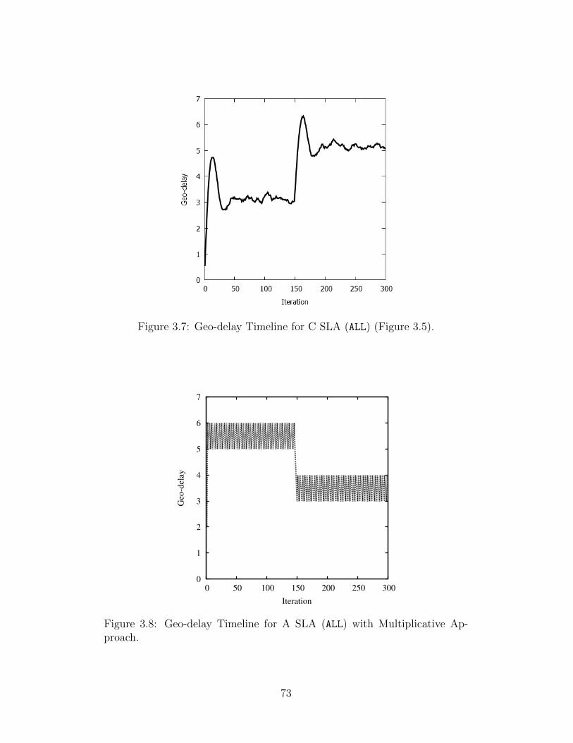
Figure 3.7: Geo-delay Timeline for C SLA (ALL) (Figure 3.5).

0

1

2

3

4

5

6

7

0 50 100 150 200 250 300

Geo

-del

ay

Iteration

Figure 3.8: Geo-delay Timeline for A SLA (ALL) with Multiplicative Ap-proach.

73

geo-delay trend compared to Figure 3.6. Comparing the two figures, we

observe that although the multiplicative strategy converges as fast the PID

approach both before and after the delay jump, the read delay value keeps

oscillating around the optimal value. Such oscillations cannot be avoided

in the multiplicative approach, since at steady state the control loop keeps

changing direction with a unit step size. Compared to the multiplicative

approach, the PID control approach is smoother and has less oscillations.

3.7 Related Work

In this section we discuss related work for our GeoPCAP system.

3.7.1 Composition

Composing local policies to form global policies is well studied in other do-

mains, for example quality of service (QoS) composition in multimedia net-

works [103], software defined network (sdn) composition [115], and so on.

Our composition techniques are aimed at consistency guarantees for geo-

distributed systems.

3.7.2 Geo-distributed Systems

Recent geo-distributed systems include Google Spanner [68] which provides

externally consistent strong transactions using gps clocks. Open source key

value stores Cassandra and Riak can also be deployed in a geo-distributed

manner. COPS/Eiger [105, 106] offer causal consistency across geo-distributed

datacenters, whereas Gemini [102] provides a mixture of strong and eventual

consistency by classifying operations as either RED (need strong consistency)

74

and BLUE (eventual consistency suffices).

3.8 Summary

In this chapter we have presented our system GeoPCAP, which is a geo-

distributed extension of PCAP from chapter 2. GeoPCAP has an adaptive

control loop that tunes control knobs to meet SLAs under WAN delay varia-

tions. GeoPCAP also leverages a formal probabilistic framework for compos-

ing consistency-latency tradeoffs of individual data-center storage instances

to characterize the global tradeoff. Realistic simulations show satisfactory

SLA conformance for GeoPCAP under WAN delay variations.

75

Chapter 4

GCVM: Software-defined Consistency GroupAbstractions for Virtual Machines

In this chapter we propose a practical scalable software-level mechanism for

taking crash-consistent snapshots of a group of virtual machines. The group

is dynamically defined at the software virtualization layer allowing us to

move the consistency group abstraction from the hardware array layer into

the hypervisor with very low overhead (∼ 50 msecs VM freeze time). This

low overhead allows us to take crash-consistent snapshots of large software-

defined consistency groups at a reasonable frequency, guaranteeing low data

loss for disaster recovery. By moving the consistency group abstraction from

hardware to software, we incur a minor performance overhead, but we gain

flexibility in managing the consistency group from the hypervisor software

level. To demonstrate practicality, we use our mechanism to take crash-

consistent snapshots of multi-disk virtual machines running two database

applications: PostgreSQL, and Apache Cassandra. Deployment experiments

confirm that our mechanism scales well with number of VMs, and snapshot

times remain invariant of virtual disk size and usage.

4.1 Introduction

Virtualization service providers are gradually transitioning towards software

defined storage architectures in their datacenters [27]. With prominent exam-

ples like VMware’s virtual volumes (vVol) abstraction [30], and Openstack

76

Swift [20] the software control plane for storage operations can be clearly

separated from the underlying hardware (e.g., storage arrays).

In traditional array based storage, a logical unit number (LUN), a unique

identifier that maps to one or more hard disks, is used as the unit of stor-

age resource management. Object storage allows virtual machine disks to

become the unit of management instead. This results in flexible software

level policy management of storage, while delegating snapshot and replica-

tion mechanisms transparently to hardware storage arrays.

For applications running across multiple VMs, storage arrays provide a

consistency group abstraction for crash-consistent snapshots of all virtual

disks attached to the VMs. The number of hardware consistency groups avail-

able for a storage array is typically limited (order of tens of groups) and ad-

ministrators must manually map virtual disks to appropriate LUNs to ensure

that they are snapshot or replicated as a group (see Figure 4.1). The number

of VMs (and virtual disks) that can benefit from array-defined consistency

groups are constrained by (1) the small fixed number of hardware/LUN-

based consistency groups, and (2) the manual mapping of virtual disks to

LUNs that administrators must (re-)do as VMs are provisioned and decom-

missioned.

We posit that the consistency group abstraction can be defined and man-

aged in the hypervisor while leveraging the snapshot capabilities of an un-

derlying storage array. We present a practical, scalable, mechanism to take

crash-consistent snapshots of a group of virtual machines, each with multiple

disks (devices) attached.

By carefully managing short (∼ 50msec), targeted, pauses of write I/O

in hypervisors managing the virtual disks in a consistency group we provide

a low-overhead, scalable and robust way to realize the consistency group

77

Figure 4.1: To manually configure a consistency group containing VM1 and VM3,the administrator has to ensure that their VMDKs are placed on storage backedby LUN1 in this example.

abstraction. Using our mechanism, we demonstrate the successful recovery of

two non-trivial applications – PostgreSQL and Apache Cassandra. Detailed

microbenchmarks and experiments on a hardware array confirm that our

mechanism scales well with number of VMs, and the total snapshot time for

a group remains invariant of virtual disk size and usage.

Thus our main contribution in this chapter is to move the consistency

group (CG) abstraction from hardware to software. In hardware, reconfig-

uring (or managing) consistency group incurs high cost. But the impact of

applications due to VM pause (availability performance) is less. For soft-

ware defined consistency groups (our proposal), we lower the reconfiguration

cost by managing groups at the hypervisor level. But we incur performance

penalty due to VM pause overhead. So the tradeoff is between reconfigura-

tion cost and application availability, and the two points in the tradeoff space

are hardware consistency groups (existing solution) and software consistency

groups (our solution).

78

4.2 Background

In this section we briefly discuss some background on disaster recovery mech-

anisms for virtual machines.

For disaster recovery purposes, replicating Virtual Machine data to a re-

mote site is a common way to make VM state available. Many storage ven-

dors, e.g., EMC, NetApp etc. usually provide replication as an additional

data service.

Strategies for replication include synchronous replication – where each

write operation must be completed at the remote target site before it is

considered complete – and asynchronous replication (also known as periodic

replication) – where a point-in-time snapshot is taken and then copied over

to the remote target site periodically. The interval between two point-in-time

snapshots is the Recovery Point Objective (RPO). Thus RPO refers to the

acceptable amount of data that may be lost due to a disaster. EMC-Mirror

View [11], NetApp SnapMirror [18] and Dell EqualLogic Replication [29] are

all existing commercial systems that provide periodic replication schemes.

This work focuses on asynchronous replication since synchronous replica-

tion can have high overheads depending on the distance between the source

and target remote site. Some storage arrays provide periodic replication

functionality via a replication consistency group. A point-in-time snapshot

of a consistency group is the union of the crash-consistent snapshots of all

member volumes. The number of consistency groups available for a storage

array is usually limited (order of tens of groups). As a result these are scarce

resources.

79

4.3 Problem Formulation

Consider an application A running across n virtual machines (VM) v1, . . . , vn.

VM vi has attached to it ni virtual machine disks (VMDK) di1, . . . , dini

. The

consistency group across all the VMs consist of∑n

i=1 ni devices (objects).

The application interacts with the VMs by issuing write operations to any

VMDK in the consistency group. Our objective is to take a snapshot of the

consistency group so that we can later recover the application state from VM

crash failures by attaching the snapshotted VMDKs to a set of remote VMs.

Crash Consistency Defined: Let w1, w2, . . . , wk be the ordered sequence

of consecutive writes issued to a consistency group CG. Let w ∈ WCG denote

that write w is persisted to a VMDK within CG, where WCG denotes the

set of all writes to CG. A snapshot SCG of CG is said to be crash-consistent,

if it captures a prefix w1, w2, . . . , wp of the set of all writes w1, w2, . . . , wk,

where p ≤ k. Formally, SCG is crash-consistent if W SCG is a prefix of WCG.

For correctness, we assume that the application follows the dependent write

principle [13] where new writes are only issued after previous writes have

been acknowledged as completed. This model of operation is common in

systems with Write-Ahead-Logs (WAL) such as databases (e.g., PostgreSQL

and Apache Cassandra) and journaling file systems (e.g., ext4).

Here, we make an important assumption about the application which is

critical for the correctness of our system (Section 4.4.4). We assume that an

application only issues new writes only after the previous write has been ac-

knowledged back to the application. If a write is lost (no acknowledgment),

then the application can retry by sending the same write again. An ap-

plication that submits concurrent writes must go through a write sequencer

before using our system for recovery. Many real world application follow such

80

a dependent write principle principle [13], e.g., databases with write-ahead

log (PostgreSQL, Apache Cassandra, SQLite), and journaling file systems

(ext4).

4.3.1 Example

We use an example of a database application with write-ahead log to ex-

plain the crash-consistency criteria. Consider a write operation issued to the

database. Internally the database issues a write (wlog−intent) to its write-

ahead-log (WAL) to indicate the pending database update. After the write

to the log completes then the actual write to the database (wdata) takes place

followed by a write to the WAL (wlog−complete) to record that the update op-

eration has completed. The application must wait for each write to complete,

i.e., the writes are sequential: Wlog−intent → Wdata → Wlog−complete. These are

dependent writes: Wlog−complete depends on the completion and acknowledg-

ment of Wdata, which in turn depends on the completion and acknowledgment

of Wlog−intent.

For correctness, a crash-consistent snapshot of a device must preserve the

write order of dependent writes. Further if Wlog−∗ and Wdata go to separate

disks (i.e., a virtual machine running the database uses one disk for storing

the database log and another disk for storing the actual tables/data) then

a crash-consistent snapshot of the disks of the database VM must contain a

prefix of the write-sequence: Wlog−intent → Wdata → Wlog−complete.

Next we discuss the design of our mechanism for crash-consistent snapshots

of a consistency group defined at the virtualization platform layer. Note that

we only rely on the information available at the hypervisor (the coordinator)

level to ensure crash-consistency. Enforcing stronger consistency guarantees

81

(e.g., application level consistency [6]) would require visibility of application

write or message dependencies and is outside the scope of this work.

Figure 4.2: Using the example of an application writing integers 1,2,3,4. Writes 1and 2 have been written to disk and acknowledged. Writes 3 and 4 are in-flight atvarious levels of the stack – the vscsi layer and the guest buffer cache respectively.A crash-consistent snapshot is only required to contain writes 1 and 2. Pause stopsthe virtual CPUs (vCPUs), which prevents additional I/Os from being issued. Stunflushes any I/O that has made it to the vSCSI layer and waits for its completion.VM Quiesce (Volume Snapshot Service) informs the File System in the GuestOperating System, via VMware tools, about the pending VM freeze, allowing thefile system to do any clean up, e.g., flushing buffered I/O that applications mighthave issued. As we go from Pause to Stun to Quiesce the amount of time it takesfor the VM’s activity to halt increases.

4.4 Design

Our VM hypervisor managed (software level) mechanism for consistency

groups builds upon three primitives.

1. First, we require a mechanism for stopping (and later resuming) the

I/O activity of a VM to its virtual disks (VMDKs).

2. Second, we need a mechanism for taking a snapshot of the current state

of a VMDK.

3. Finally we need a mechanism for replicating that snapshot (or a delta

from a previous anchor point) to a remote site.

82

4.4.1 IO Suspend/Resume Mechanism

The first primitive, the ability to stop (and later resume) the I/O activity

of a VM, is the most critical. Many hypervisors (e.g., VMware ESXi, Xen,

QEMU and Hyper-V) support this.

Figure 4.2 shows the mechanisms available on VMware’s ESXi hypervisor

– pause, stun and quiesce. The Xen, Hyper-V and QEMU hypervisors appear

to support mechanisms similar to ESXi’s stun and quiesce [16, 25, 35].

Standard virtualization platforms (e.g., vSphere, Xen, Hyper-V, QEMU)

typically have three mechanisms for stopping a VM’s I/O activity – Pause,

Stun and VM quiesce [16, 25, 35]. Pause stops the virtual CPUs (vCPUs)

of the VM preventing any further I/Os from being issued. Pause returns

immediately. Stun flushes any I/O that has made it to the Virtual SCSI

(vSCSI) layer. Stun waits for the I/O flushes to complete before returning.

VM Quiesce causes VMware Tools to quiesce the file system in the virtual

machine. Quiesce waits for I/Os buffered at the guest file system (and the

layers below) to be flushed before returning. Thus in terms of time to com-

plete, we have: Quiesce > Stun > Pause. Thus we use the relatively low-cost

Pause mechanism in our work.

4.4.2 Snapshot Mechanism

Second, we need a mechanism for taking a snapshot of the current state of a

VMDK. This mechanism is delegated to the storage backend. The efficacy of

our approach – specifically the amount of time VMs need to remain stopped

– strongly depends on the performance of the snapshot provider1. Snapshot

1Having VMs paused for too long may result in VM unavailability reports by monitoringsystems. This concern also imposes an upper bound on the time spent coordinating acrash-consistent snapshot across groups of VMs that span ESXi hosts.

83

providers that employ technology that allows for efficient snapshots, e.g.,

constant-time snapshots [55, 116], light-weight diffs/deltas etc. allow us to

significantly reduce the absolute time that a VM must remain paused.

Our work uses vVols, which means that the snapshot operation will be

delegated to the backing array.

4.4.3 Replication Mechanism

The final mechanism we need is one for replicating crash-consistent snapshots

to remote sites. For performance reasons snapshot replication needs to be

asynchronous [34]. We rely on storage arrays to replicate to a remote site. In

our experiments (in Section 4.5), we mount the snapshot of the consistency

group to a different VM to test for correctness. In a production setting, the

consistency group snapshot would be asynchronously replicated to a remote

site (e.g., vCloud Air [33] cloud), instead of just a separate VM, for disaster

recovery.

4.4.4 Model of Operation

Figure 4.3 shows how our system works. A centralized coordinator issues

Pause directives to all the ESXi hosts where the VMs that are part of a

consistency group are running. Note that pausing I/O for a specific VM is a

precise operation, whereas the vCPUs of the target VM will stop, other VMs

running on that ESXi host are unaffected. Once I/O has been paused for the

target VMs, the coordinator issues snapshot directives to all the ESXi hosts

in parallel. Once the snapshot completes, the coordinator issues UnPause

directives to all the ESXi hosts. A two-phase commit (2PC) [124] protocol

is used to robustly realize this interaction sequence.

84

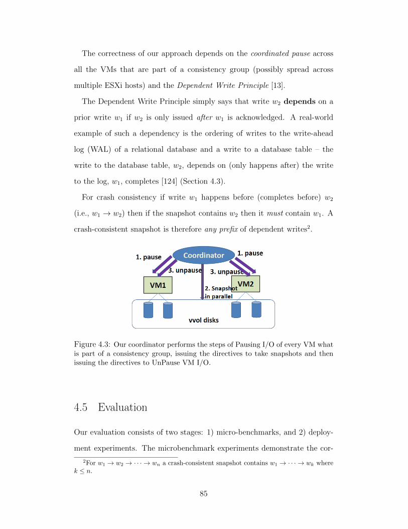
The correctness of our approach depends on the coordinated pause across

all the VMs that are part of a consistency group (possibly spread across

multiple ESXi hosts) and the Dependent Write Principle [13].

The Dependent Write Principle simply says that write w2 depends on a

prior write w1 if w2 is only issued after w1 is acknowledged. A real-world

example of such a dependency is the ordering of writes to the write-ahead

log (WAL) of a relational database and a write to a database table – the

write to the database table, w2, depends on (only happens after) the write

to the log, w1, completes [124] (Section 4.3).

For crash consistency if write w1 happens before (completes before) w2

(i.e., w1 → w2) then if the snapshot contains w2 then it must contain w1. A

crash-consistent snapshot is therefore any prefix of dependent writes2.

Figure 4.3: Our coordinator performs the steps of Pausing I/O of every VM whatis part of a consistency group, issuing the directives to take snapshots and thenissuing the directives to UnPause VM I/O.

4.5 Evaluation

Our evaluation consists of two stages: 1) micro-benchmarks, and 2) deploy-

ment experiments. The microbenchmark experiments demonstrate the cor-

2For w1 → w2 → · · · → wn a crash-consistent snapshot contains w1 → · · · → wk wherek ≤ n.

85

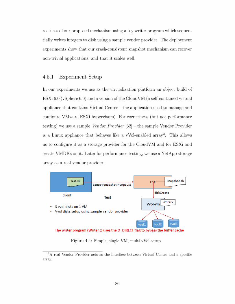
rectness of our proposed mechanism using a toy writer program which sequen-

tially writes integers to disk using a sample vendor provider. The deployment

experiments show that our crash-consistent snapshot mechanism can recover

non-trivial applications, and that it scales well.

4.5.1 Experiment Setup

In our experiments we use as the virtualization platform an object build of

ESXi 6.0 (vSphere 6.0) and a version of the CloudVM (a self-contained virtual

appliance that contains Virtual Center – the application used to manage and

configure VMware ESXi hypervisors). For correctness (but not performance

testing) we use a sample Vendor Provider [32] – the sample Vendor Provider

is a Linux appliance that behaves like a vVol-enabled array3. This allows

us to configure it as a storage provider for the CloudVM and for ESXi and

create VMDKs on it. Later for performance testing, we use a NetApp storage

array as a real vendor provider.

Figure 4.4: Simple, single-VM, multi-vVol setup.

3A real Vendor Provider acts as the interface between Virtual Center and a specificarray.

86

4.5.2 Microbenchmarks

Single VM Multiple Disk Consistency Groups

The first question we wish to answer is whether we can take a crash-consistent

snapshot of a single VM with multiple (3) VMDKs stored on vVols. Fig-

ure 4.4 shows the setup. A small script initiates the calls to pause, snapshot

and unpause. A short C-program (Writer.c) uses Direct I/O (the O DIRECT

flag) to write fixed-length records (512 bytes) containing integer data (see

Listing 4.1) while bypassing the Operating System buffer cache to files stored

on each VMDK/vVol. Figure 4.5 shows that our test program correctly

stripes writes across the 3 vVols. To verify the contents of the snapshot we

mount the snapshots of each vVol on a separate virtual machine and read

back the records written to each data file. An epoch represents a round of

writes across all (three) attached vVols.

Listing 4.1: 512 byte Record data structure of 4 byte integers

s t r u c t Record {

i n t epoch ;

i n t data ;

i n t pad [ 1 2 6 ] ; // 512 − 8 bytes

} ;

Multiple VM Multiple Disk Consistency Groups

The second question we wish to answer is whether we can take a crash-

consistent snapshot across multiple VMs on multiple ESXi hosts, each with

multiple vVols. This is shown in Figure 4.6. An extended writer program

alternates writes across the vVols of VM1 (local) and VM2 (remote) – a write

87

Figure 4.5: Simple, single-VM, multi-vVol results. Our snapshot contains writesof integers striped across the 3 vVols.

Figure 4.6: Multi-VM, multi-vVol, and multi-ESXi setup. In this setup our writerprogram alternates writing across “local” vVols and “remote” vVols.

to a vVol of VM1 is followed by a write to a vVol of VM2 before writing again

to a vVol of VM1 etc. Each epoch represents a write across all the vVols for

all the VMs. Figure 4.7 shows that a crash-consistent snapshot taken across

the vVols of VM1 and VM2 contains a prefix of the writes.

Necessity of Coordinated Pause

The third question we wish to answer is whether the coordinated Pause

is necessary. Using the multi-VM setup (Figure 4.6) we allow the writer

program to run and first take a snapshot of one disk first, and then take

snapshots (in parallel) of all the remaining disks. Figure 4.8 shows the “gaps”

(missing writes) in the union of the snapshots of each vVol, i.e., the result does

not capture a prefix of dependent writes and thus is not a crash-consistent

88

Figure 4.7: Multi-VM, multi-vVol, and multi-ESXi results. Odd integers go tothe vVols of VM1 (local) and even integers to the vVols of VM2 (remote). Thehighlighted portions represent the individual vVol snapshots that comprise thecrash-consistent snapshot of the consistency group containing VM1 and VM2.

snapshot using our correctness criteria (Section 4.3). Thus all the disks in the

consistency group must be simultaneously paused to ensure crash consistency.

Figure 4.8: Multi-VM, multi-vVol, and multi-ESXi results. Without pause, theunion of snapshot contents contains gaps (missing preceding writes) and as a resultthe result is not a crash-consistent snapshot.

89

VMDK Size (GB) Snapshot timetype time (msecs)OS 20 49

Data1 1 56Data2 10 40Data3 100 41

Table 4.1: Time to create a snapshot on VMFS for different VMDK sizes.

Overhead of VM Pause

The fourth question we wish to answer is how long a VM needs to remain

paused while we take a crash-consistent snapshot. We configure a VM with

multiple VMDKs of different sizes – ranging from 1GB, 10GB, 100GB and

measure the time taken to create the snapshot. For this experiment we

use VMware Virtual Machine File System (VMFS) [136]. Table 4.1 shows

that the time to take a snapshot is small (a few tens of milliseconds) and is

independent of the size of the VMDK. In the case of VMFS, the time to create

snapshots using redo logs depends on the number of changed sectors [31].

Later in Section 4.5.3, we also benchmark snapshot creation times for a

NetApp storage array based vVol disk.

The ability to take snapshots in parallel within and across ESXi hosts

and the relatively small snapshot creation time (depending on the snapshot

provider’s underlying technology) means that, with the appropriate snapshot

creation technology, the total amount of time VMs need to be paused can be

bounded and short.

4.5.3 Deployment Experiments

In this section we move towards reality in two aspects: (1) we replace the

toy writer application with non-trivial applications, and (2) we replace the

sample vendor provider with a real storage array (NetApp) and demonstrate

90

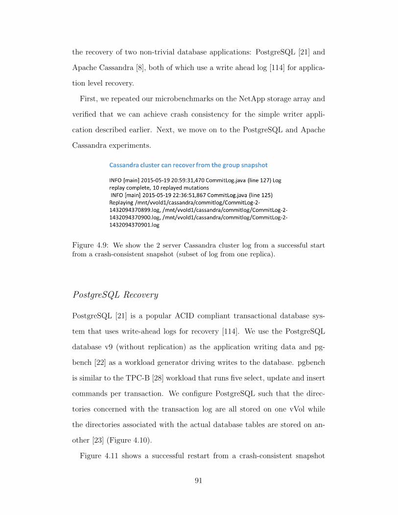
the recovery of two non-trivial database applications: PostgreSQL [21] and

Apache Cassandra [8], both of which use a write ahead log [114] for applica-

tion level recovery.

First, we repeated our microbenchmarks on the NetApp storage array and

verified that we can achieve crash consistency for the simple writer appli-

cation described earlier. Next, we move on to the PostgreSQL and Apache

Cassandra experiments.

Figure 4.9: We show the 2 server Cassandra cluster log from a successful startfrom a crash-consistent snapshot (subset of log from one replica).

PostgreSQL Recovery

PostgreSQL [21] is a popular ACID compliant transactional database sys-

tem that uses write-ahead logs for recovery [114]. We use the PostgreSQL

database v9 (without replication) as the application writing data and pg-

bench [22] as a workload generator driving writes to the database. pgbench

is similar to the TPC-B [28] workload that runs five select, update and insert

commands per transaction. We configure PostgreSQL such that the direc-

tories concerned with the transaction log are all stored on one vVol while

the directories associated with the actual database tables are stored on an-

other [23] (Figure 4.10).

Figure 4.11 shows a successful restart from a crash-consistent snapshot

91

Figure 4.10: We configure PostgreSQL 9 such that the directories associated withits transaction log are stored on one vVol and the directories associated with actualdatabase tables are stored on another vVol.

across the PostgreSQL vVols. PostgreSQL performs various integrity checks

before starting the database, and the log indicates that the integrity checks

of the snapshots were successful.

Figure 4.11: We show the PostgreSQL log from a successful start from a crash-consistent snapshot.

Apache Cassandra Recovery

Next we show we can use our mechanism to recover the state of a NoSQL

database Apache Cassandra[8], running both in centralized and distributed

modes.

We use YCSB v 0.1.4 [67, 36] to send operations to Apache Cassandra.

92

Each YCSB experiment consisted of a load phase, followed by a work phase.

Unless otherwise specified, we use the following YCSB parameters: 1 YCSB

client, 1GB data-set (1024 keys, 1 MB size values), and a write-heavy dis-

tribution (50% writes). The default key size was 10 B for Cassandra. The

default throughput was 1000 ops/s. All operations use a consistency level of

ALL.

We ran experiments in two modes: first we deploy Cassandra on a single

VM, this setup is similar to the PostgreSQL setup shown in Figure 4.10.

Second we deploy Cassandra over a cluster of 2 VMs, each VM located on

a separate ESXi host. The experiment setup is shown in Figure 4.12. For

cluster experiments, we setup 2 replicas for each key. We use YCSB to

load Cassandra with 1024 keys during the load phase, and inject read/write

operations during the work phase. Each YCSB run lasts for 60 seconds.

We configure Apache Cassandra such that the commit log directories (write-

ahead logs) and data directories were located on separate vVols. Our Cas-

sandra experiments involve vVols carved out of a 300GB NetApp storage

array.

To verify that the snapshot of write operations actually is a prefix of all

write operations, we instrument YCSB to log all operations. The operation

log file is stored in the same disk as the commit log. Each entry in the

operation log stores the key and the corresponding value for each write (put)

operation. Thus when we take a group snapshot of all VMs, we also save

as part of the snapshot, the operation log. For correctness, the snapshot

operation log file should be a proper prefix of the full operation log file

obtained at the end of the YCSB experiment.

During recovery, Apache Cassandra servers use the commit log to recover

any missing data [9]. Similar to PostgreSQL, Cassandra writes follow the

93

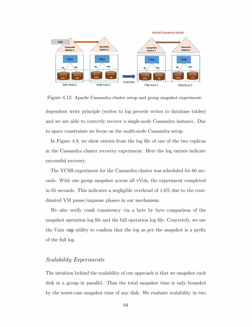
Figure 4.12: Apache Cassandra cluster setup and group snapshot experiment.

dependent write principle (writes to log precede writes to database tables)

and we are able to correctly recover a single-node Cassandra instance. Due

to space constraints we focus on the multi-node Cassandra setup.

In Figure 4.9, we show entries from the log file of one of the two replicas

in the Cassandra cluster recovery experiment. Here the log entries indicate

successful recovery.

The YCSB experiment for the Cassandra cluster was scheduled for 60 sec-

onds. With one group snapshot across all vVols, the experiment completed

in 61 seconds. This indicates a negligible overhead of 1.6% due to the coor-

dinated VM pause/unpause phases in our mechanism.

We also verify crash consistency via a byte by byte comparison of the

snapshot operation log file and the full operation log file. Concretely, we use

the Unix cmp utility to confirm that the log as per the snapshot is a prefix

of the full log.

Scalability Experiments

The intuition behind the scalability of our approach is that we snapshot each

disk in a group in parallel. Thus the total snapshot time is only bounded

by the worst-case snapshot time of any disk. We evaluate scalability in two

94

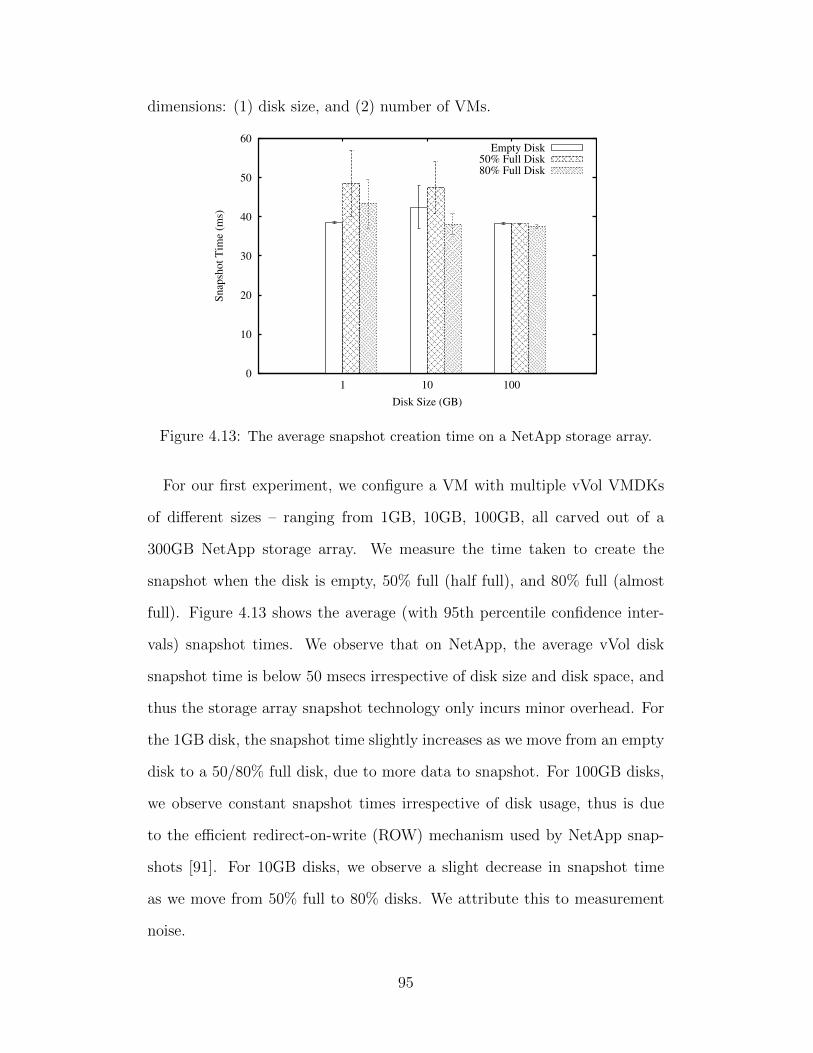
dimensions: (1) disk size, and (2) number of VMs.

0

10

20

30

40

50

60

1 10 100

Sn

apsh

ot

Tim

e (m

s)

Disk Size (GB)

Empty Disk50% Full Disk80% Full Disk

Figure 4.13: The average snapshot creation time on a NetApp storage array.

For our first experiment, we configure a VM with multiple vVol VMDKs

of different sizes – ranging from 1GB, 10GB, 100GB, all carved out of a

300GB NetApp storage array. We measure the time taken to create the

snapshot when the disk is empty, 50% full (half full), and 80% full (almost

full). Figure 4.13 shows the average (with 95th percentile confidence inter-

vals) snapshot times. We observe that on NetApp, the average vVol disk

snapshot time is below 50 msecs irrespective of disk size and disk space, and

thus the storage array snapshot technology only incurs minor overhead. For

the 1GB disk, the snapshot time slightly increases as we move from an empty

disk to a 50/80% full disk, due to more data to snapshot. For 100GB disks,

we observe constant snapshot times irrespective of disk usage, thus is due

to the efficient redirect-on-write (ROW) mechanism used by NetApp snap-

shots [91]. For 10GB disks, we observe a slight decrease in snapshot time

as we move from 50% full to 80% disks. We attribute this to measurement

noise.

95

Overall we have observed that snapshot creation times are small (about

50 msecs) and invariant with respect to the amount of data in a virtual disk

(empty, half full, 80% full). This indicates we should be able to define the

scalability constraint of a software-defined consistency group purely in terms

of the number of VMs and not in units of the amount of data in the attached

virtual disks.

0

5

10

15

20

25

30

35

40

2 4 6 8 10

Sn

apsh

ot

Tim

e (m

s)

Number of VMs

Figure 4.14: Snapshot time vs. number of VMs.

In the next experiment (Figure 4.14), we vary the number of VMs from

2 to 10, with increments of 2. Each VM had 3 disks attached to it, thus

we run experiments with a maximum consistency group size of 30. With a

distributed writer program alternatively writing consecutive integers to each

disk in the consistency group, we take group snapshots using our mechanism.

For each VM count, we measure the mean and 95th percentile confidence

interval of snapshot time for each VM in the group. Since snapshots are

done in parallel, and VM pause/unpause is instantaneous, these numbers

quantify the overhead of taking group snapshots.

We observe that the worst case snapshot time for VMs in a consistency

96

group stays below 40 ms as the number of VMs in a consistency group in-

creases. This is mainly due to efficient redirect-on-write (ROW) snapshot

mechanisms employed by the NetApp storage back-end. NetApp snapshots

are based on the WAFL (Write Anywhere File Layout) [91]. The key idea in

WAFL is to keep a set of pointers to blocks of data which enables the filesys-

tem to make copies by just copying the pointers. Thus ROW snapshots

redirect changes to new blocks, and creating a new snapshot only requires

copying volume metadata (pointers) [19]. This indicates that our proposed

crash-consistency mechanism scales well with increasing number of VMs in

a consistency group. Overall, the two scalability experiments demonstrate

that for our proposed mechanism, (1) disk size and disk space do not con-

strain scalability; (2) scalability can be defined purely in terms of number of

VMs in a consistency group; and (3) worst case snapshot overhead remains

bounded with increasing number of VMs in a consistency group. Thus we

conclude that our proposed mechanism scales well.

Consecutive Snapshots and IO Bandwidth

Any realistic application will want to take consecutive snapshots at fixed

intervals and push them to some reliable backup storage. The objective of

this experiment is to measure the impact of multiple consecutive snapshots

on application IO bandwidth. For this experiment we ran the IOzone [17]

filesystem benchmark to measure IO bandwidth with and without snapshots

issued from the hypervisor. We ran IOzone on a 10 GB disk to transfer a

256 MB file. First we ran the benchmark without any snapshots. Then we

ran the benchmark again, but in conjunction with 5 disk snapshots with 1

minute sleep time in between snapshots. This resulted in about 30% drop in

97

IO bandwidth and a modest increase in the total time for the experiment.

The relatively high bandwidth reduction with consecutive snapshots in-

dicate the possibility of optimizing consecutive snapshots. One approach

could be to only take a full snapshot for the first time, and for each consec-

utive iteration, only take a delta snapshot (i.e., the follow-up snapshots only

record the differences from the previous snapshot). Optimizing consecutive

snapshots to minimize bandwidth overhead is left as future work.

4.6 Related Work

In this section we discuss related work for our GCVM system.

4.6.1 VM Replication

There has been much work on enabling consistent replication across multiple

VMs. In host-based Replication (HBR) [34, 96], the host itself is responsible

for replication, whereas our mechanism lets hardware storage arrays take

care of replication. We extend on the HBR approach by adding coordination

across multiple ESX hosts and provide implementation and experimental

results to highlight the feasibility of our approach via an evaluation of the

scalability constraints of ensuring crash consistency for multiple VMDKs that

are spread across multiple ESX hosts.

HBR works via a HostAgent plugin that provides a way to manage and

configure VM replication and a virtual SCSI (vSCSI) filter driver that (among

other things) intercepts all VM I/O to disks and transfers replicated data to

the remote site. Rather than coordinate group consistency at this lower level

we do it in a higher layer.

It should be noted that crash-consistency is different from

98

application-level consistency [6]. Given that a crash-consistent snapshot is

the union of dependent writes it is possible that this collection of writes does

not correspond directly to a previously observed application-level state.

4.6.2 Group Abstractions

Compared to the vast literature on checkpointing of distributed programs [73],

here we look at checkpointing the state of a single application, which interacts

with multiple virtual machines. Also these techniques checkpoint in-flight

messages, whereas our mechanism ignores in-flight unacknowledged mes-

sages. Compared to hardware consistency group abstractions proposed by

NetApp and EMC [12], we move the consistency group abstraction from hard-

ware to software. Distributed process group abstractions were initially pro-

posed in [62], and later incorporated in the ISIS virtual synchrony model [53].

In both cases, the objective is to support group multicast, whereas our goal

is to checkpoint and recover a group of VMs for disaster recovery.

4.6.3 Checkpointing Distributed Applications

Many techniques have been proposed for checkpointing distributed applica-

tions. These techniques can be roughly categorized into application level

(e. g. , ARIES write ahead log mechanism [114]), library level [61, 126], and

OS level [120]. Our VM level group snapshot mechanism is closer to OS-

level checkpointing mechanisms, but our focus is on taking snapshots, and

not on migration which is complementary to our work. Application level

checkpointing requires access and modification of application source code;

our approach is application agnostic.

Note that our mechanism can take a crash consistent snapshot of a running

99

distributed system, without resorting to complicated distributed snapshot al-

gorithms (e. g. Chandy-Lamport algorithm [58]). We only use disk snapshots,

and don’t need to keep track of in-flight messages. In-flight messages are not

acknowledged by an application adhering to the dependent writes principle,

thus the application does not expect them to be part of the snapshot.

4.6.4 VM Snapshot Mechanisms

Virtualization provides a flexible solution to decouple application execu-

tion, and checkpoint/restart from the underlying physical infrastructure.

ZapC [100] is a light-weight virtualization that provides checkpointing for a

group of processes which form a process domain (pod). Compared to ZapC,

we are check-pointing VM groups. Xen on InfiniBand [127] and VNsnap [95]

both offer mechanisms to snapshot an entire virtual network environment.

We are only concerned with checkpointing VM disks.

4.6.5 Consistency Models

Crash-consistency models were first proposed in modern file systems like

EXT2, EXT3, and ZFS [55] for recovery purposes. The authors in [63] pro-

pose optimistic crash-consistency for better performance at the cost of only

probabilistic guarantees for crash-consistency. However these systems are

concerned with proper write ordering to a single disk, rather than across

multiple disks spread across VMs, as we are.

100

4.7 Summary

In this chapter we proposed a practical scalable mechanism for taking crash-

consistent snapshots of a group of virtual machines. This enabled us to

move the consistency group abstraction from hardware to software with very

low overhead (∼ 50 msecs VM freeze time). This low overhead facilitated

taking crash-consistent snapshots of large consistency groups at a reasonable

frequency. Thus our mechanism can provide low RPO for disaster recovery.

Experiments confirmed that in our mechanism, snapshot times are invariant

of disk size and disk space, and that it scales well with increasing number of

VMs.

There are a number of future research directions to pursue. First, in this

chapter we have not focused on optimizing consecutive group snapshots.

Since there is significant redundancy between consecutive snapshots, an im-

portant optimization problem is to find an optimal schedule for a sequence

of group snapshots that meets certain data loss guarantees (RPO). Second,

we rely on the dependent writes principle to ensure crash consistency. How-

ever not all applications might follow the dependent writes principle (e.g., a

multi-threaded application with multiple writer threads). We can investigate

relaxations of the dependent writes principle which could guarantee weaker

consistency models (e.g., optimistic crash consistency [63]). Weaker models

improve performance at the risk of data loss, but also require access to guest

operating system resources (e.g, guest buffers).

101

Chapter 5

OPTiC: Opportunistic graph Processing inmulti-Tenant Clusters

In this chapter, we present a system called OPTiC, or Opportunistic graph

Processing in multi-Tenant Clusters. While existing clusters can process mul-

tiple graph computations, they do not take full advantage of the multi-tenant

nature. We propose an opportunistic mechanism called PADP (Progress

Aware Disk Prefetching) for creating additional replicas of the input graph

of a job. The key idea is that the replica is placed at the servers that are

currently running the maximum progress job. This is because the maximum

progress job is most likely to complete before any other job, and free cluster

resources for the next job. Thus prefetching the input of the next waiting

job in the server(s) running the maximum progress job allows us to overlap

the graph loading time of the next waiting job, with the computation of the

current running jobs.

We utilize novel graph level metrics to identify which current running job

has made maximum progress. Thus by trading the cost of an additional

replica, we can opportunistically improve the run-time performance of jobs

by reducing the time to fetch input data from a local disk (instead of re-

mote disk) to memory. We have incorporated our technique into Apache

Giraph [3], a popular graph processing system that can run on top of Apache

YARN [4] cluster scheduler. Realistic experiments with Yahoo! and Face-

book job traces indicate our technique improves median job turnaround time

to up to 50%. To the best of our knowledge, we are the first to systematically

102

explore and optimize multi-tenant graph processing systems.

5.1 Introduction

Distributed graph processing is a popular computational framework for pro-

cessing large scale graphs with billions of vertices and trillions of edges. For

example, Pregel [109], PowerGraph [84], GraphLab [107], and LFGraph [92]

are prominent graph processing frameworks that achieve efficiency and scal-

ability. The goal of these systems is to compute important metrics (e. g.,

pagerank, shortest path, centrality) on large-scale graphs (e. g., Facebook

graph, the Web graph). These large-scale graphs typically have billions of

vertices and trillions of edges [64]. Thus distributed graph processing systems

are often deployed on large commodity clusters [110]. These frameworks usu-

ally organize a graph processing job into two phases: the graph preprocessing

phase and the computational phase. The graph preprocessing phase loads

the graph from disk, and partitions graph data into chunks, each of which is

handled by a subset (usually one) of the computation unit. The computa-

tional phase runs the actual distributed graph algorithm, and is iterative in

nature. Recent studies have shown that the graph pre-processing phase can

take significant time [92].

Despite the widespread deployment of graph processing engines on com-

modity clusters, there exists a semantic gap between the graph processing

layer and the cluster scheduling layer (Figure 5.1). For example, Apache Gi-

raph is a popular graph processing engine that runs on top of Apache Hadoop.

The Hadoop cluster scheduler (YARN) is only aware that it is processing a

map-reduce job and is unaware that it is actually a graph processing job.

Similarly the graph processing layer typically uses the entire cluster to run a

103

Figure 5.1: Semantic gap between graph processing and cluster schedulerlayers. The graph processing layer does not take full advantage of multi-tenancy of underlying cluster scheduler. The cluster scheduler is not awareof the graph nature of jobs.

single job, and once a job finishes it starts another job that will again occupy

the entire cluster. Thus both layers are unaware of any special structure or

opportunities available in the other layer. As concrete examples of available

opportunities, if the cluster layer knows that two consecutive graph process-

ing jobs (e.g., PageRank followed by Shortest Path job on the Facebook Web

Graph) share the same graph, then instead of freeing the task memory allo-

cated for the graph partitions of the first job, the cluster manager can keep

the graph partitions in memory for the next job. Thus the second job can

avoid a costly graph loading and partitioning phase, and this can result in

faster completion time for the second job.

In this chapter, we investigate for the first time the benefits of scheduling

multi-tenant graph processing jobs on a shared and over-subscribed non-

preemptive cluster. A multi-tenant cluster differs from a single-tenant cluster

in that there can be multiple jobs running simultaneously on the cluster,

thus fully utilizing the resources. The cluster scheduler serves to maximize

the overall performance and resource utilization of the jobs. In our case,

we assume that a given multi-tenant cluster is already fully occupied by

104

currently running (graph processing) jobs. We also assume the scheduler

uses a non-preemptive scheduling policy, and any upcoming jobs are placed

into a FIFO waiting-queue.

We present a system called OPTiC for Opportunistically graph Processing

on multi-Tenant Clusters. The key idea in our system is to opportunistically

overlap the graph pre-processing phase of queued jobs with the graph com-

putation phase of the current running job with maximum progress. Since

the maximum progress job is most likely to complete first, our system op-

timizes run-time performance by prefetching the graph input of the next

queued job onto the server(s) resources running the maximum progress job.

As a concrete instantiation of this technique, we propose Progress Aware Disk

Prefetching (PADP), where we prefetch the graph input of a waiting job (cre-

ate one additional replica) into the disks of server(s) running the maximum

progress job. This allows the new job to only incur a local fetch from disk to

memory, instead of a remote network fetch. Such a remote fetch would be

costly when disk bandwidth is much higher than network bandwidth, which

is a realistic scenario for today’s commodity clusters [39].

In order to decide which current running job is making maximum progress

(and is most likely to complete before others), we propose a novel progress

estimator for graph computation based on the percentage of active vertices

in a graph processing system. This allows us to estimate progress in a profile-

free and cluster agnostic manner. However our OPTiC system architecture

is general enough to work with any suitable progress estimator.

Our deployment experiments with Apache Giraph [3] running on top of

the Apache YARN [4] cluster scheduler show that we can reduce median job

turn-around time for graph processing jobs up to 50% under realistic network

and workload conditions, at the cost of one additional replica of the input

105

graph stored in the distributed file system (DFS) associated with the cluster

scheduler.

5.2 Graph Processing Background

In this section, we first give an overview of graph processing systems, and

define some key terms that we use later.

A graph processing system performs computation on a graph loaded into

the memory of a server or partitioned among a set of servers. In this chapter

we mainly deal with graphs that can be loaded entirely within the memory of

a single server. In general graph processing consists of two phases: (1) graph

loading and partitioning, and (2) graph computation. The typical life-cycle

of a graph processing job is shown in Figure 5.2.

Figure 5.2: Anatomy of a graph processing job. Phase 1: Preprocessing (loadingfrom disk and partitioning among distributed workers), Phase 2: Computation(Gather-Apply-Scatter by each vertex program), synchronize at barrier, Finallyterminate when all vertices become inactive.

106

5.2.1 Loading and Partitioning

Typically in a distributed cluster, the graph input is stored in a fixed format

in the distributed file system (DFS) associated with the cluster. For example

production Facebook graph processing systems store the graphs either in

HDFS or as Hive tables [64]. Before computation the graph must must be

fetched from disk into the memory of a single server (if there is enough

memory), or partitioned across the memory of multiple servers. Distributed

graph partitioning can take various forms: simple hash partitioning [92], or

edge based partitioning [60, 84, 125]. Both loading and partitioning the graph

can be expensive [92].

5.2.2 Computation

The synchronous, vertex-centric Gather-Apply-Scatter (GAS) style of graph

computation is the most common model, and is supported by most pop-

ular systems [64, 84, 92]. In this model, computation occurs in iterations

or supersteps, wherein vertices gather values from neighbors, aggregate and

apply the values to do local computation, and finally scatter the results to

neighbors. Supersteps are separated by global synchronization barriers. A

vertex can be in either of two states: active or inactive. At the beginning all

vertices are generally active. At any time a vertex can voluntarily enter the

inactive state or can be passively activated by an incoming message from a

neighbor. When a vertex has no more pending messages in a superstep, it

becomes inactive. The overall program terminates when all vertices become

inactive.

107

5.3 Problem Statement

Consider n graph processing jobs running on a shared cluster. We assume

a non-preemptive oversubscribed cluster, i.e., there are always jobs waiting

to be scheduled, and current jobs are not preempted. The cluster is fully

utilized by the current graph jobs. Now a new graph processing job Jnew

arrives in the system, and we need to decide where to schedule/place the

new job. Our objective to place the resources for the job (graph input file)

in a manner to improve overall job completion time performance.

5.4 Key Idea of OPTiC: Opportunistic Overlapping of

Graph Preprocessing and Computation

The key idea in OPTiC is to opportunistically overlap the graph pre-processing

phase of queued jobs with the graph computation phase of current jobs. Our

system design is based on a few assumptions. First, we assume synchronous

graph processing, where workers synchronize at a barrier at the end of each

superstep, based on the bulk synchronous parallel [137] model of computa-

tion. Second, we assume the cluster is over-subscribed; thus there is always a

job waiting to be scheduled. Third, we assume the cluster is non-preemptive;

thus there is no priority among jobs, and a waiting job cannot preempt a

running job. Finally, we assume all input graphs are stored somewhere in

a distributed file system (DFS) associated with the cluster. For example, if

the system uses the YARN cluster scheduler [4], then the input graphs could

be all stored in HDFS [15]. The key idea of OPTiC is depicted in Figure 5.3.

Assuming we have a good estimation of the progress of currently running

jobs (discussed later in Section 5.8), we want to exploit this information to

increase the performance of jobs waiting to be scheduled. Each graph pro-

108

Figure 5.3: Key idea of OPTiC: overlap the graph preprocessing phase of the nextwaiting job with the graph computation phase of the maximum progress job.

cessing job consists of a graph loading (and partitioning) phase and a com-

putational phase. By overlapping graph loading and preprocessing phase

(including graph partitioning for multiple workers), with the actual compu-

tation phase of current jobs, we can improve the run-time performance of a

sequence of graph processing jobs.

Our main technique is to utilize current progress metrics of the running

jobs to prefetch the input graph data of a job waiting in the scheduler queue

to an appropriate location in order to reduce the time to fetch the input data

for computation. Since the cluster is work-conserving, if a job is waiting,

there is no resource available to run the job. Thus instead of waiting in the

queue, we can opportunistically try to move the input data of the waiting job

closer to where the job will run next (the server(s) running the max progress

job (MPJ)). We now describe the different design stages we went through for

our system.

To implement this idea of overlapping graph pre-processing of waiting jobs

with graph computation of current jobs, we first explored progress-aware

memory prefetching techniques. The main idea was to start directly fetching

109

(and if needed, partitioning) the graph input of the next job waiting in the

queue, into the memory of the servers currently running the max progress

job (MPJ). However the problem with this approach is that since the cluster

is over-subscribed and non-preemptive, there is no free memory available to

store the prefetched graph, since all of the cluster memory is used to store

and do computation of the current running jobs.

Next we contemplated having a fixed percentage of memory in the cluster

(e.g., 20% containers in YARN) just for prefetching new graphs in memory,

while the remaining memory resources are used to run the current job. How-

ever as it turns out, this policy would have resulted in the same job schedule

as the default FIFO policy used in schedulers like YARN.

5.5 PADP: Progress Aware Disk Prefetching

The key realization at this stage was that if we cannot utilize the memory

of servers running the max progress job, we can at least try to utilize the

disk resources of those servers by prefetching the graph to disk. Suppose

based on our progress estimation, we know that Jmax is the max progress

job; that is, a future job Jnew is most likely to run on the free resource of

Jmax once it finishes. We move the input data associated with Jnew to be

locally available at the cluster resources currently allocated to Jmax, in order

to reduce the remote fetching overhead once Jnew starts. In other words, we

pre-fetch Jnew’s data into the disks of servers that Jnew is going to be run on.

Thus we create one additional replica for each chunk of the input graph for

Jnew at the servers running Jmax. We call this technique as progress aware

disk prefetching (PADP).

The PADP policy depends on one critical assumption. We assume disk

110

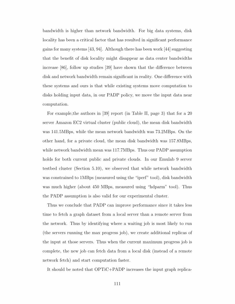
bandwidth is higher than network bandwidth. For big data systems, disk

locality has been a critical factor that has resulted in significant performance

gains for many systems [43, 94]. Although there has been work [44] suggesting

that the benefit of disk locality might disappear as data center bandwidths

increase [86], follow up studies [39] have shown that the difference between

disk and network bandwidth remain significant in reality. One difference with

these systems and ours is that while existing systems move computation to

disks holding input data, in our PADP policy, we move the input data near

computation.

For example,the authors in [39] report (in Table II, page 3) that for a 20

server Amazon EC2 virtual cluster (public cloud), the mean disk bandwidth

was 141.5MBps, while the mean network bandwidth was 73.2MBps. On the

other hand, for a private cloud, the mean disk bandwidth was 157.8MBps,

while network bandwidth mean was 117.7MBps. Thus our PADP assumption

holds for both current public and private clouds. In our Emulab 9 server

testbed cluster (Section 5.10), we observed that while network bandwidth

was constrained to 1MBps (measured using the “iperf” tool), disk bandwidth

was much higher (about 450 MBps, measured using “hdparm” tool). Thus

the PADP assumption is also valid for our experimental cluster.

Thus we conclude that PADP can improve performance since it takes less

time to fetch a graph dataset from a local server than a remote server from

the network. Thus by identifying where a waiting job is most likely to run

(the servers running the max progress job), we create additional replicas of

the input at those servers. Thus when the current maximum progress job is

complete, the new job can fetch data from a local disk (instead of a remote

network fetch) and start computation faster.

It should be noted that OPTiC+PADP increases the input graph replica-

111

tion factor from the default (3) to default(3) + at most 1 opportunistically

created replica. Although we incur increased storage and bandwidth cost to

increased replication, in reality the actual increase in dollar cost is almost

zero. This is because disk is much cheaper compared to main memory de-

vices, and most disk resources are already under-utilized. Thus with a slight

increase in replication storage cost, OPTiC+PADP policy can optimize job

completion time. Thus OPTiC+PADP trades storage cost for improved run-

time performance.

5.6 System Architecture

We now present the design of our system OPTiC for Opportunistically schedul-

ing multi-Tenant graph processing jobs in a shared Cluster, using the PADP

policy. The core idea of our system can be summarized in the following

pseudo-code.

Algorithm 1 OPTiC-PADP Core Mechanism

function Schedule(new job Gn)Step 1. Identify the current job Gp that has made maximum progress

(MPJ). Let S denote the server(s) running Gp.Step 2. Prefetch input and schedule the new job Gn to run on the

disks of Send function

Thus there are two main components of our system design in OPTiC. First

is a component that tracks the progress of all currently running jobs and

decides which job is the maximum progress job (MPJ). We discuss the graph

computation progress estimation later in section 5.8. In principle, different

progress estimators can be plugged into the modular OPTiC architecture.

Second, there is a component that prefetches resources for the next queued

job onto the MPJ server(s).

112

Figure 5.4: System Architecture.

Our overall system architecture is shown in Figure 5.4. There is a central

job queue, where jobs are queued waiting to run on the cluster. When there

are enough resources to run a new job, the graph processing engine fetches

the job from the queue in FIFO order and submits it to the cluster scheduler.

All input graphs for the jobs are already loaded in the distributed file system.

The current running jobs in the cluster periodically send their progress metric

values to the Progress Estimation Engine. For a new job fetched from the

queue, if there are enough resources, generally they will be scheduled by the

cluster scheduler on free resources (e.g., containers). The cluster scheduler

by default will try to colocate new containers with the input data. When a

job is waiting in the queue, the application coordinator for the job fetches

the information about the servers running the maximum progress job. This

data is then fed into the replication engine, which creates additional replicas

for each chunk of the waiting jobs input graph at the specified locations.

Finally when the next job in line is scheduled, it can load the graph (and

possibly partition it) from a local disk instead of incurring remote network

data transfer overheads. The OPTiC scheduling algorithm is depicted in

Figure 5.5.

113

Figure 5.5: OPTiC Scheduling Algorithm. The OPTiC scheduler lives inside thegraph processing run-time (Figure 5.4). Running jobs periodically report progressto the OPTiC scheduler. For a waiting job, the OPTiC scheduler fetches progressinformation of current jobs and uses Algorithm 2 (discussed later in Section 5.8)to decide the maximum progress job (MPJ). It then looks up the current server(s)resources S running the MPJ, and instructs the replica placement engine to placean additional replica of the waiting jobs graph input in S. The cluster schedulerindependently schedules the next job on S, when the MPJ completes.

5.7 Progress-aware Scheduling

Our system proposes a progress-aware scheduling strategy. In this section

we formalize this scheduling technique and state and prove a theorem about

the optimality of progress-aware scheduling.

In progress aware scheduling, we keep track of the current progress of each

running graph processing job. Assume the progress metrics for the n jobs

G1, G2, . . . Gn, are p1 ≥ p2 ≥ . . . ≥ pn without loss of generality. Higher val-

ues of pi means the job is closer to completion. The progress metric indicates

how much computation has been performed, and is an indicator of how long

it will take for the job to finish. Then job G1 with maximum progress p1, is

more likely to complete before any other job. Thus we can opportunistically

schedule the new job Gn+1 on the computation units (resources) currently

holding the partitions for G1. If G1 takes t1(p1) additional time to finish,

114

then Gn+1 needs to wait for t1(p1) time to start. Estimating t(p) for a job

with progress percentage p requires profiling different graph processing jobs,

and this has an overhead. We now present a theorem showing optimality of

our approach.

Theorem 5 Let p1 ≥ p2 ≥ . . . ≥ pn be the progress metric for a set of jobs

running in a work conserving non-preemptive cluster such that p1 ≥ p2 ≥

. . . ≥ pn. If the cluster has infinite bandwidth, then placing the graph dataset

of the next queued job in the server(s) currently running job with progress p1

minimizes job completion time for the next queued job.

Proof: Let the next queued job be Jnext, and the job with maximum

progress p1 be Jmax. Let Smax denote the server(s) running the computa-

tion for Jmax. Th total computation time for the new job running on S is

tStotal = tSload + tcompute. tcompute is independent of where the graph input is

fetched from. Let tSload denote the time the load the graph from server S.

Since Jnext will start on Smax, we have that tSmaxload < tSload∀S. Thus tStotal is

minimized for S = Smax. 2

This theorem makes a number of simplifying assumptions. First, we as-

sume infinite bandwidth, thus making a copy of the input graph on a new

server is instantaneous. Second, we assume that if S has more than one

server, the time to partition the graph among servers in S is negligible. For

finite bandwidth, the time to place a new replica at a destination server is

not negligible. Thus a bandwidth-aware placement policy would be to find

the maximum progress p job server(s) S such that the time to copy the graph

to S is less than the time to run the remaining computation (1 − p). The

optimality of this strategy can be proved similarly, and is left as future work.

115

5.8 Graph Computation Progress Metric Estimation

We now discuss different ways of measuring progress of graph processing jobs.

The performance of progress-aware scheduling (PADP policy in OPTiC)

depends heavily on the accuracy of graph job progress metrics, and estimat-

ing the remaining time. Such estimates allow us to decide which current

job is making maximum progress. Doing this with high accuracy results in

efficient scheduling results using OPTiC. Accurately estimating the progress

metric can be challenging, since it depends on different factors, such as graph

algorithm, the graph size, the active vertex count. Thus mathematically

the remaining time estimate ti(pi) of a graph processing job i with current

progress pi can be expressed approximately as a function of the graph al-

gorithm, and the graph size. We describe three approaches to estimating

the progress metric. We organize our discussion here by first discussing the

approaches we initially proposed and found to be inadequate. Finally we

present the design and algorithm that worked best for us. For each approach

we discuss the pros and cons.

5.8.1 Profile-based Approach

One approach to estimate graph computation progress is to profile the job

run-time characteristics of various graph algorithms on different input sizes

and different cluster configurations. Then based on these profiles, we can

estimate the progress of graph computation. For example at any given time

t, we can calculate how much time the job has been running, and use the

profiles to predict when it will complete. Machine learning techniques can

be used for such predictions. The disadvantage of this approach is the huge

profiling overhead. As a result we do not use such an approach in our system.

116

5.8.2 Utilizing Cluster Scheduler Metrics

A popular approach to graph processing is to map graph jobs to staged

dataflow jobs. For example, Apache Giraph [3] (used by Facebook), and

GraphX [85] deployed on Spark [144] (which is deployed on Mesos [90]),

both map graph processing jobs to staged data-flows, which are then effi-

ciently scheduled on a cluster scheduler like Mesos or YARN. GraphX maps

Pregel [109] jobs to a sequence of join and group-by dataflow operators,

whereas Giraph maps graph jobs to map-reduce stages.

Mature cluster schedulers like YARN have job progress estimators for each

stage. For example for both YARN map and reduce stages, we can extract the

current progress of mappers and reducers. So another approach to compare

the progress of two arbitrary graph jobs G1 and G2, would be to check their

current dataflow stage (map/reduce), and percentage complete within that

stage. So for example, if G1 is in map stage, and G2 is in reduce stage, we

say G2 has closer to completion. If both G1 and G2 are in the same stage

(e.g., reduce) then we could use the reducer percentage of the jobs to decide

which job has made more progress.

This approach is attractive since it does not require profiling. This ap-

proach is also independent of graph algorithm type and graph size. A prob-

lem with this approach is that it depends on how a graph algorithm is im-

plemented as a dataflow program. Also within a stage, progress does not

always correspond to progress of a graph job. For example Giraph graph

jobs are mapped to map-only map-reduce programs, and the map percent-

age reported by the scheduler is proportional to how much input data has

been processed. This does not directly map to iterative graph algorithms.

As a result, we do not use this approach in our system.

117

5.8.3 Profile-free Approach

Thus our goals are to avoid: (1) the overhead of profiling, and (2) the de-

pendence on the underlying cluster scheduler metrics. If we can correlate job

progress with a graph processing level metric that is independent of the plat-

form, then we can track the evolution of such a metric to infer job progress.

We choose the active vertex count percentage (AVCP) as such a metric. For a

graph processing system, the active vertex count (AVC) is defined as the num-

ber of active vertices. A vertex is said to be active if it has some un-processed

incoming message from the previous superstep (assuming synchronous graph

processing). We define the active vertex count percentage (AVCP) as the

ratio of active vertex count and total vertex count in the graph (n).

It should be noted that active vertex count is not an attribute of an ab-

stract graph algorithm, rather it is a property of a distributed implementa-

tion of such an algorithm in a graph processing platform or framework. As

long as a graph algorithm can be implemented in such a manner, we can

use AVCP to track progress. Our objective in this profile-free approach is

to estimate and compare graph computation progress without profiling and

in a cluster-agnostic manner. We wish to see how far we can go in terms

of estimating graph computation progress without any profiling. Our exper-

iments in Section 5.10.7 demonstrate the accuracy limits of the profile-free

approach.

Consider the evolution of AVCP of eight well known graph algorithms

(Pagerank, Single Source Shortest Path (SSSP), K-core Decomposition, Con-

nected Components, Undirected Triangle Count, Approximate Diameter,

Graph Laplacian, and Graph Partitioning) running on a 100 million vertex

graph using the PowerGraph [84] system, shown in Figures 5.6 - 5.12.

118

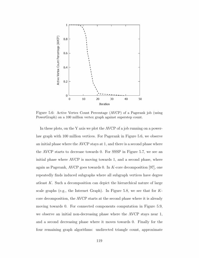
Figure 5.6: Active Vertex Count Percentage (AVCP) of a Pagerank job (usingPowerGraph) on a 100 million vertex graph against superstep count.

In these plots, on the Y axis we plot the AVCP of a job running on a power-

law graph with 100 million vertices. For Pagerank in Figure 5.6, we observe

an initial phase where the AVCP stays at 1, and there is a second phase where

the AVCP starts to decrease towards 0. For SSSP in Figure 5.7, we see an

initial phase where AVCP is moving towards 1, and a second phase, where

again as Pagerank, AVCP goes towards 0. In K-core decomposition [97], one

repeatedly finds induced subgraphs where all subgraph vertices have degree

atleast K. Such a decomposition can depict the hierarchical nature of large

scale graphs (e.g., the Internet Graph). In Figure 5.8, we see that for K-

core decomposition, the AVCP starts at the second phase where it is already

moving towards 0. For connected components computation in Figure 5.9,

we observe an initial non-decreasing phase where the AVCP stays near 1,

and a second decreasing phase where it moves towards 0. Finally for the

four remaining graph algorithms: undirected triangle count, approximate

119

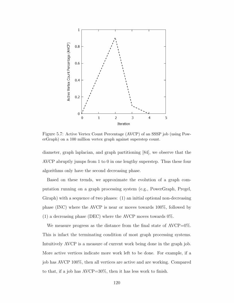
Figure 5.7: Active Vertex Count Percentage (AVCP) of an SSSP job (using Pow-erGraph) on a 100 million vertex graph against superstep count.

diameter, graph laplacian, and graph partitioning [84], we observe that the

AVCP abruptly jumps from 1 to 0 in one lengthy superstep. Thus these four

algorithms only have the second decreasing phase.

Based on these trends, we approximate the evolution of a graph com-

putation running on a graph processing system (e.g., PowerGraph, Pregel,

Giraph) with a sequence of two phases: (1) an initial optional non-decreasing

phase (INC) where the AVCP is near or moves towards 100%, followed by

(1) a decreasing phase (DEC) where the AVCP moves towards 0%.

We measure progress as the distance from the final state of AVCP=0%.

This is infact the terminating condition of most graph processing systems.

Intuitively AVCP is a measure of current work being done in the graph job.

More active vertices indicate more work left to be done. For example, if a

job has AVCP 100%, then all vertices are active and are working. Compared

to that, if a job has AVCP=30%, then it has less work to finish.

120

Figure 5.8: Active Vertex Count Percentage (AVCP) of a k-Core Decompositionjob (using PowerGraph) on a 100 million vertex graph against superstep count.

We can now describe the algorithm to compare progress of two jobs. The

basic idea is as follows. Consider two jobs J1, J2 with AVCP values a1, a2,

0 ≤ a1, a2 ≤ 1. We have three cases:

1. Case 1: If J1 is in the initial non-decreasing (INC) phase, and J2 is in the

second decreasing (DEC) phase, then we conclude J2 is the maximum

progress job (MPJ).

2. Case 2: If both J1 and J2 are in the INC phase [0%-100%], and a1 < a2,

then J2 is the MPJ.

3. Case 3: If both J1 and J2 are in the DEC phase[100%-0%], and a1 > a2,

then J2 is the MPJ.

Consider two jobs in the same phase (e.g. DEC phase) with AVCP values

of 40% and 50%. Both these jobs have similar progress. Although, the job

121

Figure 5.9: Active Vertex Count Percentage (AVCP) of an Connected Compo-nents job (using PowerGraph) on a 100 million vertex graph against superstepcount.

with 40% AVCP is most likely to finish first, the rate of decrease of AVCP

can vary, and the job with 50% could end up finishing slightly before the

job with AVCP 40%. To account for this, we divide each phase into equal

intervals. For example we can divide the DEC interval into three disjoint

sub-intervals H = [100% − 67%], M = [67% − 33%],L = [33% − 0%]. We

order the sub-intervals in terms of progress towards AVCP=0% (termination)

as: L > M > H. Thus for two jobs in different intervals (job 1 in L, job 2 in

M), we use this ordering to decide the maximum progress job (job 1). For

two jobs in the same sub-interval (both in M), we toss a coin and randomly

pick a job as the max progress job. This randomness allows us to deal with

different rates of decrease of AVCP. The case where both jobs are in the INC

phase is similarly handled.

The overall algorithm for comparing the progress of two graph processing

122

Figure 5.10: Active Vertex Count Percentage (AVCP) of an Undirected TriangleCount job (using PowerGraph) on a 100 million vertex graph against superstepcount.

jobs at time t (usually the last superstep time) is shown in Algorithm 2.

The algorithm first checks whether the jobs are in INC or DEC phases

(lines 5-14) by comparing AVCP at time t and t − 1 (the last two recorded

super-step times). If AVCP decreases by more than a threshold (e.g., ε =

10%), then the job is in DEC phase, otherwise it is in the initial INC phase.

If they are in different phases, then the job in DEC phase wins and is the

MPJ (lines 15-20). Otherwise, if both jobs are in the same INC phase (lines

21-31), then the interval is divided into I sub-intervals, and we check which

sub-intervals contain AV CP for each job. The job in the later sub-interval

(based on the order) is returned as the MPJ. In case both jobs are in the

same sub-interval, we randomly choose a job as the MPJ (lines ). The case

when both jobs are in DEC phase is similar (lines 32-42).

123

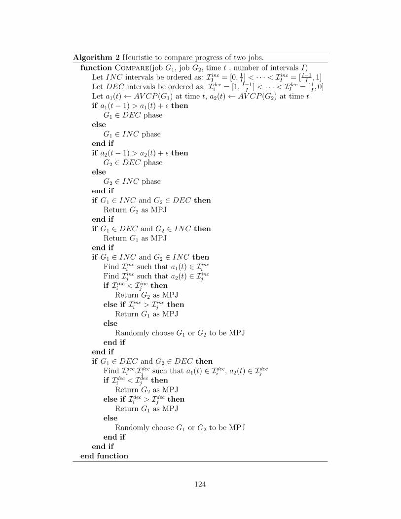
Algorithm 2 Heuristic to compare progress of two jobs.

function Compare(job G1, job G2, time t , number of intervals I)Let INC intervals be ordered as: I inc1 = [0, 1

I] < · · · < I incI = [ I−1

I, 1]

Let DEC intervals be ordered as: Idec1 = [1, I−1I

] < · · · < IdecI = [1I, 0]

Let a1(t)← AV CP (G1) at time t, a2(t)← AV CP (G2) at time tif a1(t− 1) > a1(t) + ε then

G1 ∈ DEC phaseelse

G1 ∈ INC phaseend ifif a2(t− 1) > a2(t) + ε then

G2 ∈ DEC phaseelse

G2 ∈ INC phaseend ifif G1 ∈ INC and G2 ∈ DEC then

Return G2 as MPJend ifif G1 ∈ DEC and G2 ∈ INC then

Return G1 as MPJend ifif G1 ∈ INC and G2 ∈ INC then

Find I inci such that a1(t) ∈ I inci

Find I incj such that a2(t) ∈ I incj

if I inci < I incj thenReturn G2 as MPJ

else if I inci > I incj thenReturn G1 as MPJ

elseRandomly choose G1 or G2 to be MPJ

end ifend ifif G1 ∈ DEC and G2 ∈ DEC then

Find Ideci ,Idecj such that a1(t) ∈ Ideci , a2(t) ∈ Idecj

if Ideci < Idecj thenReturn G2 as MPJ

else if Ideci > Idecj thenReturn G1 as MPJ

elseRandomly choose G1 or G2 to be MPJ

end ifend if

end function

124

Figure 5.11: Active Vertex Count Percentage (AVCP) of an Approximate Di-ameter job (using PowerGraph) on a 100 million vertex graph against superstepcount.

5.8.4 Variations of the Profile-free Approach

In the profile-free approach we estimate progress by tracking the evolution

of AVCP. For two jobs, the job with AVCP closer to the terminal 0% is

considered the max progress job. One variation is to estimate the actual job

finish time, given current AVCP. We can use regression of curve-fitting to do

this. The drawback of this approach is that different jobs can have different

rates of change for AVCP. Thus a simple linear regression would not suffice,

and might require profiling which we want to avoid.

Another variation is to keep track of first and second derivatives of AVCP

(rate of change of AVCP or velocity, and acceleration). This would increase

the overhead of tracking progress, and it is not guaranteed that the job with

highest velocity and acceleration towards AVCP=0% will finish first.

125

Figure 5.12: Active Vertex Count Percentage (AVCP) of a Graph Laplacian job(using PowerGraph) on a 100 million vertex graph against superstep count.

5.8.5 Generality of the Profile-free Approach

Our profile-free approach is motivated by the observed evolution of AVCP

for four popular graph analytics algorithms shown in Figures. We believe

the technique is general and applicable for a wider range of graph analytics

algorithms including (1) triangle count (2) approximate diameter (3) group

source shortest paths, (4) k-means clustering, and many more. The reason

this is true is that all these algorithms have been implemented in graph

processing frameworks like PowerGraph [84] and Giraph [3], where the job

terminating condition is AVCP=0%. Thus our technique would work for

these algorithms.

126

Figure 5.13: Active Vertex Count Percentage (AVCP) of a Graph Partitioningjob (using PowerGraph) on a 100 million vertex graph against superstep count.

5.8.6 Accuracy of the Profile-free Approach

We now characterize workload conditions that lead to high accuracy for our

profile-free approach. Our goal is to understand the limits of the profile-free

approach.

The Algorithm works well for same type of graph jobs (e.g., SSSP)

with different sizes. Consider two SSSP jobs on input graphs with 10K

and 100K vertices respectively. Both jobs have the same amount of resource

allocated to them. Since the maximum active vertex count of the 10K job is

smaller, at any time, it will be closer to termination compared to the 100K

job. Thus progress comparison algorithm works well in this case.

The Algorithm works well for different types of jobs with similar

run-times. Consider comparing the progress of an SSSP job with a K-core

127

job. If both jobs have similar run-times, then most likely during comparison,

both jobs will be in the DEC phase. Thus the algorithm correctly predicts

the MPJ in this case.

The Algorithm works poorly for different types of jobs with vastly

different run-times. This tells us the limit of the profile free approach.

Consider an SSSP job with estimated run-time T , and a K-core job with

estimated run-time at-least 10 × T Thus with equal resources allocated to

both jobs, the SSSP job will always finish earlier than K-core. However

SSSP has an INC phase before the DEC phase, whereas K-core starts at

the DEC phase. Thus, if at the time of comparison, SSSP is in the first

phase, then our algorithm mis-predicts K-core as the max progress job, even

though SSSP always finishes first. This demonstrates that the profile-free

approach starts to break down for different types of jobs with different run-

time characteristics. We can remedy this by telling the system that k-core is

always slower than SSSP, but that approach would no longer be profile-free.

5.9 Implementation

We have implemented a scheduler prototype that supports our PADP policy

for the Apache Giraph [3] graph processing system on top of an Apache

YARN [4] cluster.

5.9.1 Incorporating Multi-tenancy in Giraph

While Giraph can be deployed on top of YARN, it is not truly a multi-

tenant graph processing system. To simultaneously schedule multiple graph

processing jobs on YARN, we would need to run multiple separate Giraph

128

instances, one for each job. We made modifications to Giraph such that

multiple graph processing jobs can be scheduled using a single Giraph run-

time. We use a Java thread-pool for this purpose. We implemented a console

for submitting new jobs to the Giraph run-time. The console interface parses

every job command and delivers it to the scheduling component. Each newly

submitted job is handed of to a new thread in the thread-pool.

5.9.2 PADP Policy Implementation

Our PADP policy relies on two key pieces of information from the graph

processing systems: active message count (which we normalize to get AVCP)

and allocated containers for any currently running jobs. In Apache Giraph,

these two information are available in the master node. The master node will

aggregate active message count at each superstep, and for each job this aggre-

gated value (Phase and Interval, Section 5.8.3) is propagated to a centralized

log in the cluster. Also, in Giraph whenever a new container is allocated, we

also propagate the information to a centralized log in the cluster. These val-

ues are therefore globally available in a centralized server so that the OPTiC

scheduler can utilize them to schedule future jobs.

There are two approaches to disseminate AVCP and container information

in the system: push and pull. In the push approach, the running jobs pe-

riodically send AVCP and container logs to the central master server. We

use this push approach in our prototype implementation. In some scenarios,

a pull method might fare well. In a pull method, whenever the scheduler

needs AVCP and container logs, it requests such information from the mas-

ter nodes, or from the ApplicationMaster of all currently jobs. One benefit

of the push approach is that it reduces repeated communication overhead

129

when there are a lot of incoming jobs. The downside of the push approach is

that these logs must be aggregated and stored in a centralized manner and

this creates a central point of failure. The centralized server can be made

fault-tolerant using state machine replication [128] technique. We leave such

fault tolerance techniques for future work.

5.9.3 HDFS Replication

To exploit the progress information of current jobs, we wish to pre-fetch

the input data into the local disks of the maximum progress job. In our

prototype, suppose we have an incoming job j with input graph data G and

the maximum progress job j∗ with associated machines M , we do the pre-

fetching by creating a copy of G at each host in M , so that when j starts at

the same machines of j∗, it can use the data that is already locally available.

Our prototype is built in Hadoop ecosystem and uses HDFS as the un-

derlying distributed file system (DFS). To create the additional replica, we

make an explicit copy (with replication factor 1) of G using HDFS’s native

file copy feature and place it in the disk of M . Thus we do not interfere with

the default three replicas created by HDFS for every block of data. Thus our

technique does not tamper with the default fault-tolerance level of HDFS.

5.9.4 Scheduler Implementation

Our PADP policy implementation proceeds as follows. Given a waiting job

j, first it attempts to submit j to the YARN scheduler. We poll the YARN

REST API to check whether the job is in RUNNING state in the cluster. If

it is not in RUNNING state, we deduce that YARN currently does not have

adequate resources to run j. It is for such jobs j that we wish to utilize the

130

PADP policy.

To implement PADP, the scheduler proceeds by first sending requests to

YARN asking for a list of currently running jobs. For each job ji, it retrieves

the centralized progress log associated with ji and extracts the phase (INC or

DEC), and interval within the phase (Section 5.8.3). It then uses Algorithm 2

to determine the MPJ j∗. Next, it retrieves the list of allocated container(s)

of j∗. It chooses one of the containers in the list, ssh’es into the container, and

creates an HDFS file copy. This copy is created locally created at the server

running that container. After the copy process is finished, the scheduler kills

the original job j, and resubmits it but with the updated path of the copied

input graph (the additional replica). The detailed algorithm is shown in

Algorithm 3.

5.10 Evaluation

We performed our experiments on an Emulab [140] clusters with 9 quad-core

servers, each with 64GB memory. We use delay emulation to mirror the

network delays typically observed in a single data-center environment [52].

We implemented the PAPD policy and incorporated it into Apache Giraph

graph processing framework (version 1.10) [3] running on top of the Hadoop

YARN Cluster (version 2.7.0) [4].

We configure one server as the Master which runs the YARN resource man-

ager (RM) and the HDFS name node (NN), while the remaining 8 servers act

as slaves and contain node manager (NM), and data nodes (DN). Each slave

has 1 8GB memory container, thus the total YARN cluster has 64GB memory

for running jobs. We assume all input graph data are stored in the Hadoop

Distributed File System (HDFS) [132], which is the default distributed stor-

131

Algorithm 3 Implementation of PADP Policy in Giraph+YARN

function PADP(J: newJob, yarnManager)G ← J.inputPathyarnManager.submit(J)status ← yarnManager.getStatus(J)if status = Queued then

yarnManager.kill(J)K ← yarnManager.getCurrentJobs()maxProgress ←<> . Empty Tuple.maxProgressJob ← nullfor all k ∈ K do

progress =< phase, interval > ← readProgressLog(k) . Readphase and interval (See Algorithm 2).

if progress > maxProgress thenmaxProgress ← progressmaxProgressJob ← k

end ifend forM ← readContainerLog(maxProgressJob)for all m ∈ M do

ssh(m).HDFS-copy(G,concat(G,”copy”))end forJ.inputPath ← concat(G,”copy”)yarnManager.submit(J)

end ifend function

132

age system used in conjunction with Apache YARN [4]. The average disk

bandwidth of the cluster (measured using “’hdparm’) is 450MBps, while the

average network bandwidth (measured using “iperf”) is 1MBps.

Our main performance metric is job turn-around time (TAT), defined as

the difference between job finish time and job arrival time in the queue. Our

cost metric is replication factor (RF) of the input graphs stored in DFS. We

compare our OPTiC PADP policy (P ) with the YARN baseline FIFO policy

(B). The baseline policy cost is the default replication factor in DFS (3),

whereas the cost of PADP is default(3) + at most 1 opportunistically created

replica. We measure performance improvement of our PADP (P ) policy over

the baseline (B) as B−PB× 100%.

We conduct five set of experiments. First, we vary the network delay

conditions in the cluster using realistic delay distributions for a data-center

network [52] and measure the performance of PAPD and baseline policies

(Figure 5.14, Figure 5.15). For this experiment, we always use a fixed size

graph input for all jobs and set a constant inter-arrival time between suc-

cessive jobs. For the next set of experiments, we move towards reality by

(1) generating job sizes that represent a realistic workload (Facebook Map-

reduce cluster workload) [143] (Figure 5.18), and (2) setting the inter-arrival

time between jobs to be exponentially distributed. For the third experiment,

we use a larger production trace from Yahoo! with job size and arrival time

values (Figure 5.19). Next, we define a metric called graph commonality,

which measures how the different jobs share graph inputs. We vary this

metric to evaluate PADP and baseline policies (Figure 5.20). In this exper-

iment, we also vary the job sizes to evaluate the scalability of our system.

For the final experiment, we test how our system works with a heterogeneous

mix of different graph algorithms, and measure the limits of the profile-free

133

approach (Figure 5.21, Figure 5.22).

5.10.1 Input Graphs

We conduct our experiments on large randomly generated undirected graphs.

Uniform graphs are randomly generated in the way that the probability of

an edge existing between any pair of vertices is the same. The uniform graph

assumption does not impact our results, and we would get similar conclusions

with Power-law graphs[74] of the same size. The reason is that our techniques

are not targeted at or optimized for Power-law graphs. We expect them to

work arbitrary graph inputs.

5.10.2 Test Graph Algorithm

We conduct most of our experiments on a distributed version of single source

shortest path algorithm. Unless otherwise specified, this is the default graph

processing job in our experiments. The pseudo-code of the algorithm is given

in Algorithm 2, written in the semantics of Apache Giraph[3].

5.10.3 Impact of Realistic Network Delays

For this set of experiments, we use a lognormal distribution to emulate net-

work delay conditions within a data-center network. In reality, a multi-tenant

graph processing cluster is more likely to be deployed over a data-center net-

work. Thus we make the network delays more practical in this setting. The

network delays are set using a log-normal distribution, based on a recent

measurement study of network characteristics in a single data-center [143].

We vary the lognormal distribution mean from 1ms to 4ms, and the standard

deviation from 0.1ms to 0.4ms. This results in average network delay values

134

Algorithm 4 Algorithm for single source shortest path in Apache Giraphsemantics

function VertexCompute(self,incomingMessages)if getSuperstep() = 0 then

self.dist ← 0end ifif self = getSourceVertex() then

minDist ← 0else

minDist ←∞end iffor all m ∈ incomingMessages do

minDist ← min(m.getValue(), minDist)end forif minDist < self.dist then

self.dist ← minDistfor all e ∈ self.getEdges() do

d ← e.getWeight() + minDistsendMessage(e.getTargetVertex(), d)

end forend ifvoteToHalt()

end function

135

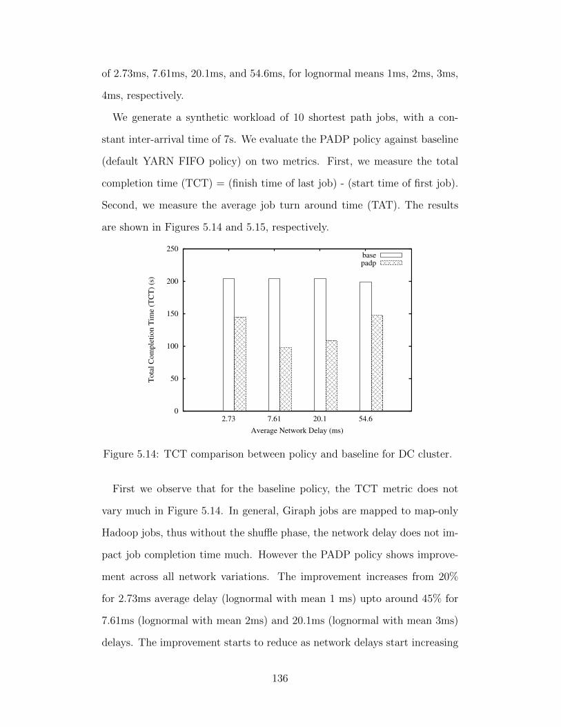
of 2.73ms, 7.61ms, 20.1ms, and 54.6ms, for lognormal means 1ms, 2ms, 3ms,

4ms, respectively.

We generate a synthetic workload of 10 shortest path jobs, with a con-

stant inter-arrival time of 7s. We evaluate the PADP policy against baseline

(default YARN FIFO policy) on two metrics. First, we measure the total

completion time (TCT) = (finish time of last job) - (start time of first job).

Second, we measure the average job turn around time (TAT). The results

are shown in Figures 5.14 and 5.15, respectively.

0

50

100

150

200

250

2.73 7.61 20.1 54.6

To

tal

Co

mp

leti

on

Tim

e (T

CT

) (s

)

Average Network Delay (ms)

basepadp

Figure 5.14: TCT comparison between policy and baseline for DC cluster.

First we observe that for the baseline policy, the TCT metric does not

vary much in Figure 5.14. In general, Giraph jobs are mapped to map-only

Hadoop jobs, thus without the shuffle phase, the network delay does not im-

pact job completion time much. However the PADP policy shows improve-

ment across all network variations. The improvement increases from 20%

for 2.73ms average delay (lognormal with mean 1 ms) upto around 45% for

7.61ms (lognormal with mean 2ms) and 20.1ms (lognormal with mean 3ms)

delays. The improvement starts to reduce as network delays start increasing

136

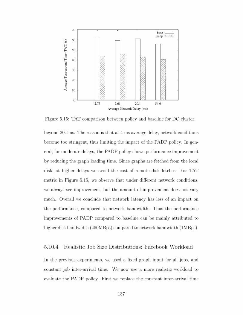
0

10

20

30

40

50

60

70

2.73 7.61 20.1 54.6

Av

erag

e T

urn

-aro

un

d T

ime

(TA

T)

(s)

Average Network Delay (ms)

basepadp

Figure 5.15: TAT comparison between policy and baseline for DC cluster.

beyond 20.1ms. The reason is that at 4 ms average delay, network conditions

become too stringent, thus limiting the impact of the PADP policy. In gen-

eral, for moderate delays, the PADP policy shows performance improvement

by reducing the graph loading time. Since graphs are fetched from the local

disk, at higher delays we avoid the cost of remote disk fetches. For TAT

metric in Figure 5.15, we observe that under different network conditions,

we always see improvement, but the amount of improvement does not vary

much. Overall we conclude that network latency has less of an impact on

the performance, compared to network bandwidth. Thus the performance

improvements of PADP compared to baseline can be mainly attributed to

higher disk bandwidth (450MBps) compared to network bandwidth (1MBps).

5.10.4 Realistic Job Size Distributions: Facebook Workload

In the previous experiments, we used a fixed graph input for all jobs, and

constant job inter-arrival time. We now use a more realistic workload to

evaluate the PADP policy. First we replace the constant inter-arrival time

137

distribution with an exponential distribution with mean 7s. Next we, sample

job sizes from a production Mapreduce cluster at Facebook [143].

We are not aware of any measurement studies or realistic workload analy-

sis of multi-tenant graph processing clusters. We believe the Facebook work-

load trace is realistic for multiple reasons. First, specifically Giraph jobs are

mapped to map-reduce jobs, thus a map-reduce workload job size distribution

should closely match Giraph graph processing workloads. Second, and more

generally, we conjecture that many Internet facing companies (especially so-

cial networking companies like Facebook, LinkedIn, Pinterest) running graph

processing jobs on a multi-tenant cluster should observe a similar workload

distribution, where most jobs are small, and only few large jobs exist.

For Facebook, running a massive Pagerank computation is atleast a daily

necessity, since the Facebook graph is constantly evolving. This would be

one large graph processing job that might take up most of cluster resources.

However Facebook also need to do targeted advertising or recommendations

to specific groups of people. This would require clustering the massive Face-

book graph in to groups of people based on some common interest of pattern.

A community detection [119] algorithm (another large job) could be used for

this purpose. Or optionally, groups formed by members could serve as the

required clustering of the graph. Once the graph is clustered into groups,

Facebook needs to extract exponentially many subgraphs corresponding to

these groups (many short jobs), and run targeted recommendation algorithms

on each subgraphs (many short jobs). Thus we conclude that a workload with

mostly short jobs, and few long jobs (not negligible) is a realistic workload

for multi-tenant graph processing1.

1We are not aware of any workload analysis studies of commercial graph processingsystems.

138

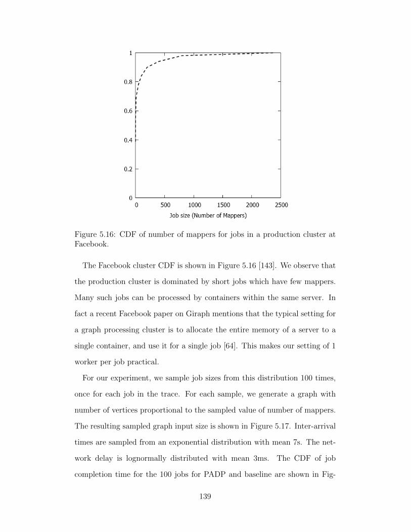
Figure 5.16: CDF of number of mappers for jobs in a production cluster atFacebook.

The Facebook cluster CDF is shown in Figure 5.16 [143]. We observe that

the production cluster is dominated by short jobs which have few mappers.

Many such jobs can be processed by containers within the same server. In

fact a recent Facebook paper on Giraph mentions that the typical setting for

a graph processing cluster is to allocate the entire memory of a server to a

single container, and use it for a single job [64]. This makes our setting of 1

worker per job practical.

For our experiment, we sample job sizes from this distribution 100 times,

once for each job in the trace. For each sample, we generate a graph with

number of vertices proportional to the sampled value of number of mappers.

The resulting sampled graph input size is shown in Figure 5.17. Inter-arrival

times are sampled from an exponential distribution with mean 7s. The net-

work delay is lognormally distributed with mean 3ms. The CDF of job

completion time for the 100 jobs for PADP and baseline are shown in Fig-

139

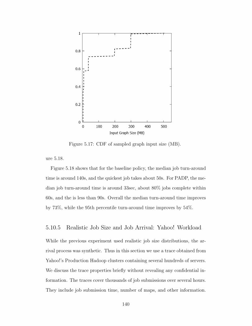
Figure 5.17: CDF of sampled graph input size (MB).

ure 5.18.

Figure 5.18 shows that for the baseline policy, the median job turn-around

time is around 140s, and the quickest job takes about 50s. For PADP, the me-

dian job turn-around time is around 33sec, about 80% jobs complete within

60s, and the is less than 90s. Overall the median turn-around time improves

by 73%, while the 95th percentile turn-around time improves by 54%.

5.10.5 Realistic Job Size and Job Arrival: Yahoo! Workload

While the previous experiment used realistic job size distributions, the ar-

rival process was synthetic. Thus in this section we use a trace obtained from

Yahoo!’s Production Hadoop clusters containing several hundreds of servers.

We discuss the trace properties briefly without revealing any confidential in-

formation. The traces cover thousands of job submissions over several hours.

They include job submission time, number of maps, and other information.

140

Figure 5.18: Job Completion Time (s) CDF for Facebook Trace (job-size)using Baseline and PADP Policy.

The jobs are of different sizes, the arrivals are bursty, and the load varies over

time. Thus this trace captures realistic mix of conditions for a multi-tenant

cluster.

We are not aware of any studies of graph processing jobs running on a

shared cluster. Thus like the previous Facebook trace experiment, we set the

graph size to be proportional to number of mappers in our experiment. We

injected 1 hour of traces with 300 jobs into our 9-server test cluster configured

with 8 containers (each server has 1 8GB container). The network delay is

about 20ms between two servers, based on a log normal distribution of mean

3ms. Figure 5.19 shows the job run-time CDF for both baseline and PADP

policies. We observe that for PADP, the median job completion time is

around 27s, compared to the median of around 63s for baseline. The 95th

percentile run-time for baseline is around 190s, whereas it is around 55s for

141

PADP. Thus PADP reduces median turn-around time for jobs by 47% and

also reduces the 95th percentile turnaround time by 48%. It does so under

realistic network and workload conditions.

Figure 5.19: Job Completion Time (s) CDF for Yahoo Trace (job size andinter-arrival time) using Baseline and PADP Policy.

5.10.6 Scalability and Impact of Commonality of Graphs

In this section, we explore how our system scales with increased graph sizes,

and increased sharing of graphs by different jobs. We first define a new

metric called graph commonality, and denote it as g. g roughly captures

the extent to which different jobs share the same graph. Thus, for example,

g = 100% indicates that all the jobs share (do computation on) the same

graph. g = 50% indicates half the jobs share one graph, the rest share

another graph. g = 0% indicates no sharing, thus each job has its own input

graph. In this next experiment, we vary g and evaluate the PADP policy

142

against baseline. We use a trace of 50 jobs with a Poisson arrival process

with mean 7s. Network delay is log-normal with mean 3ms. For g = 100%

we use one graph of size 50K vertices. For g = 50% we use two graphs of size

50K and 25K vertices. For g = 25% we use four graphs of size 50K, 25K,

16K, and 12K vertices. Finally for g = 0%, we use a separate graph for each

job varying in size from 1K upto 50K vertices. The results are shown as a

box plot in Figure 5.20.

The X axis shows commonality values for both PADP and baseline, and

the Y axis shows job completion time (TAT). Each box represents the min-

imum, 1st quartile, median, 3rd quartile, and 95th percentile values for job

completion time for the 50 job trace. We first observe that the job completion

time scales linearly with increased commonality. At 100% g, job completion

times are significantly high for the baseline. This is partly due to the larger

job-sizes (each has 50K input). But the main reason for worse performance

is that as more jobs share the same graph in disk (higher values for g), they

simultaneously try to fetch the same graph into memory, which creates disk

contention. The PADP policy avoids this contention by creating the addi-

tional replicas for jobs, and alleviates the single points of disk contention.

The average job size also increases from left to right in this plot. For

g = 0%, the average job size is 25K, whereas for g = 100% it is 50K.

Thus the plot indicates that the PADP policy also scales much better with

increased job size, compared to the baseline policy.

5.10.7 Impact of Job Heterogeneity

So far all our experiments were performed with a homogeneous trace of jobs

of the same type. In this section, we see how PADP performs with a mixture

143

Figure 5.20: Job Completion Time (s) Box Plot (Minimum, First Quartile,Median, Third Quartile, 95th Percentile) against Graph Commonality (mea-sure of how input graphs are distributed among jobs) for Baseline and PADPPolicy.

of different types of jobs. We experiment with a trace of 20 jobs with 80%

SSSP and 20% K-core jobs. The job inter-arrival time is Poisson with mean

7s, and network delay is lognormally distributed with mean 3ms. The job

run-time CDF is shown in Figure 5.21. We observe that although PADP

is competitive with baseline, there is not much performance improvement.

The reason is that with vastly differing run-times, the progress comparison

algorithm mis-predicts the max progress job.

Next we make the run-time of K-core comparable to SSSP, by using more

distributed workers for K-core. The resulting job run-time CDF is shown

in Figure 5.22. Now we see improved performance. Especially the median

turn-around time for PADP improves by 82%, while the 95th percentile turn-

around time improves by 70%. The reason for improvement is that with

144

Figure 5.21: Job Completion Time (s) CDF for for Baseline and PADP Policywith 80% SSSP and 20% k-core jobs. Run-time of k-core at-least 10 timesrun-time of SSSP.

different job types but similar run-times, the progress comparison algorithm

is more likely to correctly predict the max progress job. The similar run-

times for SSSP and K-core mean that both jobs are more likely to be in the

same DEC phase during comparision.

Thus this experiment confirms that for different types of job, the PADP

policy works well when job run-times are similar, but starts to mis pre-

dict the max progress job when run-times start to vary significantly. This

points towards an adaptive mechanism to remedy this drawback. We can

continuously measure the standard deviation of job run-times. When the

deviation is below a threshold, we use our profile-free approach. However

when the threshold is exceeded we incorporate some profiling information in

the system (e.g., K-core is always slower than SSSP). However, this adaptive

145

Figure 5.22: Job Completion Time (s) CDF for for Baseline and PADPPolicy with 80% SSSP and 20% k-core jobs. Run-times of k-core and SSSPare similar.

approach will no longer be completely profile-free anymore.

5.11 Discussion

In this section we discuss variations and extensions of the OPTiC system.

5.11.1 Experiments with Larger Partitioned Graphs

In our current experiments, the graph input file sizes are bounded by 500MB,

and can be run within 1 container. Our job sizes are motivated by a pro-

duction cluster trace [143]. However in reality we might incur much larger

graphs that will be partitioned across servers. To deal with larger graphs,

we can extend the PADP policy. Instead of storing the entire new graph file

146

replica at the single max progress server, we can use an existing partitioning

algorithm to partition the new graph across the max progress servers. This

would ensure that when the first waiting job is ready to run after the maxi-

mum progress job finishes, each server can fetch its assigned partition locally

from its attached disk. This is left as future work.

5.11.2 OpTiC for Distributed Machine Learning

The OPTiC architecture can be applied to distributed machine learning jobs,

provided we plug in a suitable progress estimator into the architecture. For

example many machine learning jobs have mathematical convergence crite-

ria, and we can check how far an algorithm is from convergence, and use

such a distance metric to measure progress. On the other hand many ma-

chine learning algorithms (e.g., k-means clustering, Latent Dirichlet Alloca-

tion (LDA) [54], Alternating Least Squares (ALS) [93]) have already been

implemented as distributed algorithms in graph processing frameworks like

Giraph [64] and PowerGraph [84]. For such distributed implementations,

our current OPTiC system with our PADP policy and profile-free progress

estimator can be used without modification.

5.11.3 Theoretical Framework for OpTiC

If we have complete oracle knowledge of all jobs that will be submitted to

the cluster, and we assume infinitely divisible computation resources (e.g.,

YARN containers can be of size infinitely small), then it is possible to math-

ematically formulate the OPTiC scheduling problem as a mathematical opti-

mization problem (most likely a mixed integer linear program (MILP)). Such

theoretical models could help us understand the the limits of our scheduling

147

algorithm. We leave such mathematical modeling as interesting future work.

5.11.4 SLO-aware OPTiC

While we optimize run-time performance in OPTiC, we do not explicitly

meet performance service level objectives (SLO). We can extend the design

of OPTiC to make it SLO-aware. In the original OPTiC mechanism, we

prefetch the next waiting job input graph onto the server(s) running the

max progress job. While the server(s) running the max progress job are

guaranteed to have at-least one unit of resource (e.g., one YARN container),

that might not be enough to meet SLOs. We can use profiling to estimate

how many containers are required for the new waiting job to meet the SLO.

Using our progress estimation and comparison engine, we can already order

the current running jobs in descending order or progress (p). For n current

running jobs J1, J2, . . . , Jn, let the ordered sequence be p1 > p2 > . . . > pn.

For OPTiC, we always choose the servers running the job with progress p1.

For SLO-aware OPTiC, we need to choose the first job Jk with progress pk

such that the server(s) running Jk have enough resources (containers) to meet

the SLO.

5.12 Related Work

In this section we discuss related work for our OPTiC system.

5.12.1 Graph Processing Systems

Google designed the first distributed graph processing system called Pregel [109]

based on message passing. Subsequently, GraphLab [107] proposed shared

148

memory style graph computation. PowerGraph [84] improved upon GraphLab

by optimizing for Power-law graphs. In particular it proposed edge-based par-

titioning algorithms based on vertex-cuts to optimize the graph partitioning

phase. LFGraph [92] improves performance using cheap hash-based parti-

tioning and a publish-subscribe based message flow architecture. XStream

[79] looks at edge centric processing for graphs. Systems have also explored

disk optimizations for single host processing in GraphChi [99]. Presto [138]

unifies graph computation and machine learning algorithms by expressing

them in terms of matrix computations, and develop a distributed array im-

plementation for doing matrix computations. Compared to all these systems,

OPTiC, for the first time, improves performance for multi-tenant graph pro-

cessing systems.

5.12.2 Multi-tenancy

Multi-tenancy has been explored in the context of cluster schedulers like

YARN [4], Mesos [90]. Natjam [65] explores multi-level eviction policies

to incorporate priorities and deadlines in a constrained map-reduce cluster.

Like Natjam, we also assume a constrained over-subscribed cluster. Unlike

Natjam, we assume no preemption. Compared to these three systems, we

are the first to explore multi-tenancy for a cluster running graph processing

jobs, instead of arbitrary dataflow (map-reduce) jobs. Pisces [131] explores

multi-tenant storage systems. Compared to Pisces, we explore multi-tenancy

for graph processing systems.

149

5.12.3 Progress Estimation for Jobs

There is a rich literature of progress estimators for map-reduce jobs and

DAGs of map-reduce jobs [117, 118]. Compared to these progress estimators,

we propose a novel progress metric for graph jobs utilizing graph level metrics

which are independent of how such graph jobs are mapped to map-reduce

jobs in many graph processing frameworks like Giraph [3], and GraphX [85].

Progress estimation for database queries has been a very fruitful area of re-

search. Progress estimators like DNE (Driver Node Estimator), and TGN

(Total Get Next) estimate progress by calculating the fraction of tuples out-

put so far by operators in a query plan [59]. Similar to database query

estimators, we estimate graph computation progress by measuring amount

of work done in terms of the percentage of active vertices (working vertices)

in a graph.

5.13 Summary

In our study, we explore the potential performance benefits to gain from op-

portunistically scheduling graph processing jobs on multi-tenant graph pro-

cessing systems. We propose a profiling-overhead free and cluster-agnostic

approach to estimate the progress of a graph processing job using a graph

level metric (Active Vertex Count). Using this metric to compare the progress

of multiple jobs, we propose a progress-aware scheduling policy (PADP) that

schedules incoming jobs based on the progress of all currently running jobs

on the cluster. For realistic workloads, we found that our progress-aware disk

prefetching (PADP) policy can outperform baseline default scheduling in a

multi-tenant cluster. Results indicate that the PADP policy in our system

OPTiC reduces median and 95th percentile job turn-around time for realistic

150

workload and network conditions. Our system also scales well with increased

job sizes and increased sharing among graphs.

151

Chapter 6

Conclusion and Future Work

6.1 Summary

In this thesis, we have demonstrated adaptive and opportunistic mechanisms

for navigating the cost-performance tradeoff space to meet desired tradeoffs

for modern cloud systems, including distributed key-value storage systems,

cloud-based disaster recovery systems, and multi-tenant graph processing

systems. In doing so, we have presented the design, implementation, and

evaluation of four systems.

Our first contribution, PCAP is an adaptive distributed storage system.

The foundation of the PCAP system is a probabilistic variation of the classi-

cal CAP theorem, which quantifies the (un-)achievable envelope of probabilis-

tic consistency and latency under different network conditions characterized

by a probabilistic partition model. Our PCAP system proposes adaptive

mechanisms for tuning control knobs to meet desired consistency-latency

tradeoffs expressed in terms in service-level agreements.

Our second system, GeoPCAP is a geo-distributed extension of PCAP. In

GeoPCAP, we propose generalized probabilistic composition rules for com-

posing consistency-latency tradeoffs across geodistributed instances of dis-

tributed key-value stores, each running on separate datacenters. GeoPCAP

also includes a geo-distributed adaptive control system that adapts new con-

trols knobs to meet SLAs across geo-distributed data-centers.

152

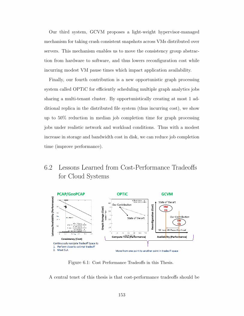
Our third system, GCVM proposes a light-weight hypervisor-managed

mechanism for taking crash consistent snapshots across VMs distributed over

servers. This mechanism enables us to move the consistency group abstrac-

tion from hardware to software, and thus lowers reconfiguration cost while

incurring modest VM pause times which impact application availability.

Finally, our fourth contribution is a new opportunistic graph processing

system called OPTiC for efficiently scheduling multiple graph analytics jobs

sharing a multi-tenant cluster. By opportunistically creating at most 1 ad-

ditional replica in the distributed file system (thus incurring cost), we show

up to 50% reduction in median job completion time for graph processing

jobs under realistic network and workload conditions. Thus with a modest

increase in storage and bandwidth cost in disk, we can reduce job completion

time (improve performance).

6.2 Lessons Learned from Cost-Performance Tradeoffs

for Cloud Systems

Figure 6.1: Cost Performance Tradeoffs in this Thesis.

A central tenet of this thesis is that cost-performance tradeoffs should be

153

considered as first class citizens when designing cloud systems. In this section

we discuss how explicitly thinking about and characterizing cost performance

tradeoffs allows as to build better cloud systems.

The various cost performance tradeoffs considered in this thesis are de-

picted in Figure 6.1. For PCAP (Chapter 2) and GeoPCAP (Chapter 3),

the tradeoff is between consistency (X axis) and latency/availability (Y axis)

(left plot in Figure 6.1). The straight lines represent the optimal tradeoffs

and the cluster of points represent the tradeoffs achieved by the PCAP sys-

tem. For these storage systems, characterizing the optimal tradeoff allowed

us to understand the limits of the storage system. This in turn allowed us to

explicitly try to perform close to the optimal envelope, in addition to meeting

SLAs. Thus an explicit characterization of the tradeoffs informed efficient

navigation of the tradeoff space to perform close to the optimal envelope.

For GCVM (Chapter 4), the key abstraction is to checkpoint and replicate

a group of virtual machines as a single unit. The state of the art hardware so-

lution has high reconfiguration cost to change the membership of the group,

whereas our proposed software solution reduces reconfiguration cost at the

modest impact of application availability (right most plot in Figure 6.1). Ex-

plicitly mapping out the tradeoff space for this system allows us to consider

future systems that lie in this tradeoff space. For example, can we build a

hybrid software-hardware solution that has reconfiguration cost in between

the pure hardware and pure software solutions, and with performance impact

lower than the software solution? Only by explicitly thinking about the cost-

performance tradeoff space, can we think of such systems in the future. It

also allows us to conjecture performance characteristics of such new systems.

For example, by looking at the explicit tradeoff space, we can conjecture that

a hybrid hardware-software solution for group consistent snapshots for vir-

154

tual machines can incur a performance penalty (VM pause time) somewhere

around 20-30 msec.

For OPTiC (Chapter 5), the tradeoff is between the graph computation

run-time and the storage replication cost (middle plot in Figure 6.1). Com-

pared to existing systems, we improve run-time at a slight increase in storage

cost. Like GCVM, this explicit tradeoff space allows us to think about other

solution points in the tradeoff space. Unlike PCAP, where we know the

optimal tradeoff, here we do not know what is the optimal solution with low-

est storage cost and best run-time performance. Explicitly placing state of

the art and our proposed solutions in the tradeoff space allows us to consider

optimal tradeoffs (like PCAP optimal tradeoffs), and understand the implica-

tions of new system designs points with different cost-performance tradeoffs.

For example the trend seems to indicate that by increasing replication factor

beyond 4, we can get even lower performance. Thus the tradeoff space allows

us to reason about optimal tradeoffs for these graph processing systems.

6.3 Future Work

We suggest several directions for future research related to this thesis.

6.3.1 Probabilistic Tradeoff Analysis for DistributedTransactional Systems

One theoretical research topic could be to explore probabilistic tradeoffs for

transaction systems. This would include probabilistic isolation models for

transactions that capture transactional semantics of different isolation mod-

els. PCAP characterizes and adapts the consistency-latency tradeoff space

for distributed key-value storage systems through a probabilistic lens. Key-

155

value stores have a simple data model. There is a value associated with a key.

However many modern NewSQL [42, 141] storage systems have more struc-

ture, and support richer abstractions like distributed transactions. While

this will not be a new transactional model, it could help us understand the

space of models better, and understand the performance impact (through-

put, fairness, contention) of various isolation levels better. Equipped with

such probabilistic tradeoff analysis, we can explore adaptive mechanisms for

meeting various performance and/or consistency requirements based on user

SLA/SLO under workload and network variations.

6.3.2 Adaptive GCVM

It would be interesting to explore adaptive mechanisms that switch between

crash consistency and application consistency based on application workload.

In GCVM, we have proposed a software level consistency group abstraction.

One direction to pursue would be to adaptively tune the consistency group

semantics to meet different objectives. For example crash consistency might

not be enough for some applications, and we might need stronger guaran-

tees such as application consistency. However stronger guarantees are costly

to maintain and impact application performance more (e.g., to ensure each

snapshot is application consistent would require VMs to be paused longer

than crash consistency requirements), thus increasing the duration between

consecutive snapshots (RPO). For example when the application workload is

light (low rate of writes), it could tolerate longer pauses and get application

consistent snapshots. But when the write-rate increases, we should not pause

for long, thus we need to switch back to cheaper crash consistency snapshots.

156

6.3.3 Extensions of OPTiC

OPTiC is concerned with efficient co-scheduling of multiple graph analytics

jobs sharing a cluster. There are many avenues of future directions to con-

sider, some of which have been mentioned already in the relevant chapter.

Here we discuss a few more directions.

Data-aware Policies

The main mechanism in OPTiC is to place additional replicas for a queued

graph job to reduce graph fetching time by utilizing progress metrics of cur-

rent jobs. Such progress aware policies are not the only available opportu-

nities in a distributed graph processing cluster. For example, we can also

explore data aware strategies. If we know that a consecutive job will be

running on a graph already in use by a current job, then we can save graph

loading time by keeping that graph in memory for the subsequent job. This

requires techniques to cache map-reduce containers, and we can utilize exist-

ing frameworks like Apache Tez [5] to investigate such mechanisms.

PADP for Arbitrary Dataflow Frameworks

We believe that the Progress Aware Disk Prefetching (PADP) can be appli-

cable for computational frameworks beyond graph processing, for example,

distributed machine learning jobs or generalized dataflow computations. The

challenge is to develop general metrics for estimating progress of arbitrary

jobs. This seems like a hard problem.

In the OPTiC graph progress estimator we use a graph level metric, active

vertex count that helps us gauge current progress. Can we find such metrics

for machine learning jobs? Many machine learning jobs have convergence cri-

157

teria that define termination. We can utilize such criteria to decide which job

will finish earlier. This also opens up the possibility of investigating various

distance metrics that define the distance to termination. Some dataflow/-

graph systems let applications specify a maximum number of iterations. This

makes it easy to check progress.

Overall it seems like estimating progress is very much application specific,

and a better architecture should separate the policy concern of application

progress (applications can use call-back mechanisms to tell the run-time how

to measure progress), whereas the actual mechanism for utilizing the progress

data to tune the performance is confined withing the system.

Distributed Extensions of OPTiC

In OPTiC, we have mainly explored graph processing jobs with one worker.

Thus the graph is not partitioned and distributed across workers. A dis-

tributed extension of OPTiC where each graph processing job is distributed

across servers is an immediate extension worth exploring.

158

References

[1] Activo: “Why Low Latency Matters?”. http://www.activo.com/

why-low-latency-does-matter-and-increases-online-sales/,last visited 2016-07-04.

[2] Amazon: milliseconds means money. http://www.uiandus.com/

blog/2009/2/4/amazon-milliseconds-means-money.html, last vis-ited 2016-07-04.

[3] Apache Giraph. http://giraph.apache.org/, last visited 2016-07-04.

[4] Apache Hadoop Yarn. http://hadoop.apache.org/docs/current/

hadoop-yarn/hadoop-yarn-site/YARN.html, last visited 2016-07-04.

[5] Apache Tez. https://tez.apache.org/, last visited 2016-07-04.

[6] Application vs. crash consistency. http://www.n2ws.com/blog/

ebs-snapshots-crash-consistent-vs-application-consistent.

html, last visited 2016-07-04.

[7] Basho Riak. http://basho.com/riak/, last visited 2016-07-04.

[8] Cassandra. http://cassandra.apache.org/, last visited 2016-07-04.

[9] Cassandra commit log architecture. http://wiki.apache.org/

cassandra/ArchitectureCommitLog, last visited 2016-07-04.

[10] Consistency in Amazon S3. http://shlomoswidler.com/2009/12/

read-after-write-consistency-in-amazon.html, last visited 2016-07-04.

[11] Emc mirror view knowledgebook. http://goo.gl/8VjTRK, last visited2016-07-04.

[12] EMC SRDF consistency groups. http://goo.gl/wBlgZQ, last visited2016-07-04.

[13] Emc srdf/a multi-session consistency on z/os. http://goo.gl/81HuZe,last visited 2016-07-04.

159

[14] Facebook userbase. http://newsroom.fb.com/company-info/, lastvisited 2016-07-04.

[15] Hadoop distributed file system (hdfs). https://hadoop.apache.org/docs/r1.2.1/hdfs_design.html, last visited 2016-07-04.

[16] Hyper-V snapshots vs. VSS snapshots explained. http://goo.gl/

5ia37H, last visited 2016-07-04.

[17] IOzone filesystem benchmark. http://www.iozone.org/, last visited2016-07-04.

[18] Netapp snapmirror data replication. http://www.netapp.com/

us/products/protection-software/snapmirror.aspx, last visited2016-07-04.

[19] Netapp snapshots. http://community.netapp.com/t5/Technology/

Are-All-Snapshots-Created-Equal/ba-p/83211, last visited 2016-07-04.

[20] Openstack Swift. http://docs.openstack.org/developer/swift/,last visited 2016-07-04.

[21] PostgreSQL. http://www.postgresql.org/, last visited 2016-07-04.

[22] PostgreSQL benchmarking tool. http://www.postgresql.org/docs/devel/static/pgbench.html, last visited 2016-07-04.

[23] PostgreSQL database physical storage. http://www.postgresql.org/docs/9.3/static/storage-file-layout.html, last visited 2016-07-04.

[24] Project Voldemort. http://www.project-voldemort.com/

voldemort/, last visited 2016-07-04.

[25] QEMU features/snapshots. http://wiki.qemu.org/Features/

Snapshots, last visited 2016-07-04.

[26] Real-time ad impression bids using Dy-namoDB. http://aws.amazon.com/blogs/aws/

real-time-ad-impression-bids-using-dynamodb/, last visited2016-07-04.

[27] The software-defined data center (sddc). http://www.vmware.com/

software-defined-datacenter/, last visited 2016-07-04.

[28] Transaction processing performance council, TPC-B. http://www.

tpc.org/tpcb/, last visited 2016-07-04.

160

[29] Understanding data replication between dell equallogic ps series groups.http://goo.gl/Ioxdv8, last visited 2016-07-04.

[30] Vmware , virtual volumes. http://www.vmware.com/products/

virtual-volumes, last visited 2016-07-04.

[31] VMware Inc., disk chaining and redo logs. https://goo.gl/6dxM16,last visited 2016-07-04.

[32] VMware VASA. http://blogs.vmware.com/vsphere/2011/08/

a-sneak-peek-at-how-vmwares-storage-partners-are-using-vasa.

html, last visited 2016-07-04.

[33] VMware vCloud Air. http://vcloud.vmware.com/

service-offering/disaster-recovery, last visited 2016-07-04.

[34] VMware vSphere Replication 6.0. https://www.vmware.com/files/

pdf/vsphere/VMware-vSphere-Replication-Overview.pdf, lastvisited 2016-07-04.

[35] Xen snapshots halting I/O. http://discussions.citrix.com/

topic/263681-xen-snapshots-halting-io/, last visited 2016-07-04.

[36] Yahoo! cloud serving benchmark (YCSB). https://github.com/

brianfrankcooper/YCSB/wiki, last visited 2016-07-04.

[37] Yahoo! cloud serving benchmark (ycsb) workloads. https:

//github.com/brianfrankcooper/YCSB/wiki/Core-Workloads, lastvisited 2016-07-04.

[38] Cassandra multi data-center deployment,2011. http://www.datastax.com/dev/blog/

deploying-cassandra-across-multiple-data-centers, lastvisited 2016-07-04.

[39] Cristina L. Abad, Yi Lu, and Roy H. Campbell. Dare: Adaptive datareplication for efficient cluster scheduling. In Proc. IEEE Cluster Com-puting, pages 159–168, 2011.

[40] Daniel Abadi. Consistency tradeoffs in modern distributed databasesystem design: CAP is only part of the story. IEEE Computer,45(2):37–42, 2012.

[41] Ittai Abraham and Dahlia Malkhi. Probabilistic quorums for dynamicsystems. In Distributed Computing, volume 18, pages 113–124, 2005.

[42] Marcos K. Aguilera, Joshua B. Leners, and Michael Walfish. Yesquel:Scalable sql storage for web applications. In Proc. ACM SOSP, pages245–262, 2015.

161

[43] Ganesh Ananthanarayanan, Sameer Agarwal, Srikanth Kandula, Al-bert Greenberg, Ion Stoica, Duke Harlan, and Ed Harris. Scarlett:Coping with skewed content popularity in mapreduce clusters. In Proc.ACM Eurosys, pages 287–300, 2011.

[44] Ganesh Ananthanarayanan, Ali Ghodsi, Scott Shenker, and Ion Sto-ica. Disk-locality in datacenter computing considered irrelevant. InProc. USENIX HotOS, pages 12–12, 2011.

[45] Masoud Saeida Ardekani and Douglas B. Terry. A self-configurablegeo-replicated cloud storage system. In Proc. USENIX OSDI, pages367–381, 2014.

[46] K. J. Astrom and T. Hagglund. PID Controllers: Theory, Design, andTuning, 2nd Ed. 1995.

[47] Hagit Attiya and Jennifer L. Welch. Sequential consistency versuslinearizability. In ACM Transactions on Computer Systems (TOCS),volume 12, pages 91–122, 1994.

[48] Peter Bailis and Ali Ghodsi. Eventual consistency today: Limitations,extensions, and beyond. In ACM Queue, volume 11, pages 20:20–20:32,2013.

[49] Peter Bailis, Shivaram Venkataraman, Michael J. Franklin, Joseph M.Hellerstein, and Ion Stoica. Pbs at work: Advancing data managementwith consistency metrics. In Proceedings of the 2013 ACM SIGMODInternational Conference on Management of Data (SIGMOD), pages1113–1116, New York, New York, USA, 2013.

[50] Peter Bailis, Shivaram Venkataraman, Michael J. Franklin, JosephM.Hellerstein, and Ion Stoica. Quantifying eventual consistency with pbs.In The Very Large Data Bases (VLDB) Journal, volume 23, pages 279–302, 2014.

[51] R. Baldoni, C. Marchetti, and A. Virgillito. Impact of wan channel be-havior on end-to-end latency of replication protocols. In Proc. EDCC,pages 109–118, 2006.

[52] Theophilus Benson, Aditya Akella, and David A. Maltz. Network trafficcharacteristics of datacenters in the wild. In Proc. ACM SIGCOMMIMC, pages 267–280, 2010.

[53] Kenneth P. Birman. The process group approach to reliable distributedcomputing. CACM, 36(12):37–53, 1993.

[54] David M. Blei, Andrew Y. Ng, and Michael I. Jordan. Latent dirichletallocation. JMLR, 3:993–1022, 2003.

162

[55] Jeff Bonwick, Matt Ahrens, Val Henson, Mark Maybee, and Mark Shel-lenbaum. The zettabyte file system. Technical report, Sun Microsys-tems, 2003.

[56] Eric Brewer. A certain freedom: Thoughts on the CAP theorem. InProc. ACM PODC, pages 335–335, 2010.

[57] Eric A. Brewer. Towards robust distributed systems (Invited Talk). InProc. ACM PODC, 2000.

[58] K. Mani Chandy and Leslie Lamport. Distributed snapshots: deter-mining global states of distributed systems. ACM TOCS, 3(1):63–75,1985.

[59] Surajit Chaudhuri, Vivek Narasayya, and Ravishankar Ramamurthy.Estimating progress of execution for sql queries. In Proc. ACM SIG-MOD, pages 803–814, 2004.

[60] Rong Chen, Jiaxin Shi, Yanzhe Chen, and Haibo Chen. Powerlyra:Differentiated graph computation and partitioning on skewed graphs.In Proc. ACM Eurosys, pages 1:1–1:15, 2015.

[61] Y. Chen, K. Li, and J.S. Plank. Clip: a checkpointing tool for messagepassing parallel programs. In Proc. ACM/IEEE SC, pages 33–33, 1997.

[62] David R. Cheriton and Willy Zwaenepoel. Distributed process groupsin the v kernel. ACM TOCS, 3(2):77–107, 1985.

[63] Vijay Chidambaram, Thanumalayan Sankaranarayana Pillai, An-drea C. Arpaci-Dusseau, and Remzi H. Arpaci-Dusseau. Optimisticcrash consistency. In Proc. ACM SOSP, pages 228–243, 2013.

[64] Avery Ching, Sergey Edunov, Maja Kabiljo, Dionysios Logothetis,and Sambavi Muthukrishnan. One trillion edges: Graph processingat facebook-scale. Proc VLDB Endowment, pages 1804–1815, 2015.

[65] Brian Cho, Muntasir Rahman, Tej Chajed, Indranil Gupta, CristinaAbad, Nathan Roberts, and Philbert Lin. Natjam: Design and eval-uation of eviction policies for supporting priorities and deadlines inmapreduce clusters. In Proc. ACM SoCC, pages 6:1–6:17, 2013.

[66] Adrian Cockcroft. Dystopia as a service (Invited Talk). In Proc. ACMSoCC, 2013.

[67] Brian F. Cooper, Adam Silberstein, Erwin Tam, Raghu Ramakrishnan,and Russell Sears. Benchmarking cloud serving systems with YCSB.In Proc. ACM SoCC, pages 143–154, 2010.

163

[68] James C. Corbett et al. Spanner: Google’s globally-distributeddatabase. In Proc. USENIX OSDI, pages 251–264, 2012.

[69] A Davidson, A Rubinstein, A Todi, P Bailis, and S. Venkatara-man. Adaptive hybrid quorums in practical settings, 2013.http://goo.gl/LbRSW3.

[70] Jeff Dean. Design, Lessons and Advice from Building Large DistributedSystems, 2009.

[71] Giuseppe DeCandia, Deniz Hastorun, Madan Jampani, GunavardhanKakulapati, Avinash Lakshman, Alex Pilchin, Swaminathan Sivasub-ramanian, Peter Vosshall, and Werner Vogels. Dynamo: Amazon’shighly available key-value store. In Proc. ACM SOSP, pages 205–220,2007.

[72] Maria Eleftheriou and Marios Mavronicolas. Linearizability in the pres-ence of drifting clocks and under different delay assumptions. In Dis-tributed Computing, volume 1693, pages 327–341. 1999.

[73] E. N. (Mootaz) Elnozahy, Lorenzo Alvisi, Yi-Min Wang, and David B.Johnson. A survey of rollback-recovery protocols in message-passingsystems. ACM Computing Survey, 34(3):375–408, 2002.

[74] Michalis Faloutsos, Petros Faloutsos, and Christos Faloutsos. Onpower-law relationships of the internet topology. ACM SIGCOMMCCR, 1999.

[75] Hua Fan, Aditya Ramaraju, Marlon McKenzie, Wojciech Golab, andBernard Wong. Understanding the causes of consistency anomalies inapache cassandra. In Proc. VLDB Endowment, volume 8, pages 810–813, 2015.

[76] Armando Fox and Eric A. Brewer. Harvest, yield, and scalable tolerantsystems. In Proc. HotOS, pages 174–178, 1999.

[77] Bugra Gedik., Scott Schneider, Martin Hirzel, and Kun-Lung Wu. Elas-tic scaling for data stream processing. In IEEE TPDS, volume 25, pages1447–1463, 2014.

[78] Seth Gilbert and Nancy A. Lynch. Perspectives on the CAP theorem.IEEE Computer, 45(2):30–36, 2012.

[79] Lewis Girod, Yuan Mei, Ryan Newton, Stanislav Rost, Arvind Thia-garajan, Hari Balakrishnan, and Samuel Madden. Xstream: a signal-oriented data stream management system. Proc. IEEE ICDE, pages1063–1189, 2008.

164

[80] Lisa Glendenning, Ivan Beschastnikh, Arvind Krishnamurthy, andThomas Anderson. Scalable consistency in Scatter. In Proc. ACMSOSP, pages 15–28, 2011.

[81] Wojciech Golab, Xiaozhou Li, and Mehul A. Shah. Analyzing con-sistency properties for fun and profit. In Proc. ACM PODC, pages197–206, 2011.

[82] Wojciech Golab, Muntasir Raihan Rahman, Alvin AuYoung, KimberlyKeeton, and Indranil Gupta. Client-centric benchmarking of eventualconsistency for cloud storage systems. In Proc. IEEE ICDCS, pages493–502, 2014.

[83] Wojciech Golab and John Johnson Wylie. Providing a measure rep-resenting an instantaneous data consistency level, January 2014. USPatent Application 20,140,032,504.

[84] Joseph E. Gonzalez, Yucheng Low, Haijie Gu, Danny Bickson, andCarlos Guestrin. Powergraph: Distributed graph-parallel computationon natural graphs. In Proc. USENIX OSDI, pages 17–30, 2012.

[85] Joseph E. Gonzalez, Reynold S. Xin, Ankur Dave, Daniel Crankshaw,Michael J. Franklin, and Ion Stoica. Graphx: Graph processing in adistributed dataflow framework. In Proc. USENIX OSDI, pages 599–613, 2014.

[86] Albert Greenberg, James R. Hamilton, Navendu Jain, Srikanth Kan-dula, Changhoon Kim, Parantap Lahiri, David A. Maltz, Parveen Pa-tel, and Sudipta Sengupta. Vl2: A scalable and flexible data centernetwork. In Proc. ACM SIGCOMM, pages 51–62, 2009.

[87] Joseph L. Hellerstein, Yixin Diao, Sujay Parekh, and Dawn M. Tilbury.Feedback Control of Computing Systems. John Wiley & Sons, 2004.

[88] Jiannong Cao Jian Lu Hengfeng Wei, Yu Huang. Almost strongconsistency: ”good enough” in distributed storage systems, 2015.http://arxiv.org/abs/1507.01663.

[89] Herodotos Herodotou, Fei Dong, and Shivnath Babu. No one (cluster)size fits all: Automatic cluster sizing for data-intensive analytics. InProc. ACM SoCC, pages 18:1–18:14, 2011.

[90] Benjamin Hindman, Andy Konwinski, Matei Zaharia, Ali Ghodsi, An-thony D. Joseph, Randy Katz, Scott Shenker, and Ion Stoica. Mesos:A platform for fine-grained resource sharing in the data center. InProc. USENIX NSDI, pages 295–308, 2011.

165

[91] Dave Hitz, James Lau, and Michael Malcolm. File system design foran nfs file server appliance. In Proc. USENIX WTEC, pages 19–19,1994.

[92] Imranul Hoque and Indranil Gupta. Lfgraph: Simple and fast dis-tributed graph analytics. In Proc. ACM SIGOPS TRIOS, pages 9:1–9:17, 2013.

[93] Yifan Hu, Yehuda Koren, and Chris Volinsky. Collaborative filteringfor implicit feedback datasets. In Proc. IEEE ICDM, pages 263–272,2008.

[94] Michael Isard, Vijayan Prabhakaran, Jon Currey, Udi Wieder, KunalTalwar, and Andrew Goldberg. Quincy: Fair scheduling for distributedcomputing clusters. In Proc. ACM SOSP, pages 261–276, 2009.

[95] A. Kangarlou, P. Eugster, and Dongyan Xu. Vnsnap: Taking snap-shots of virtual networked environments with minimal downtime. InProc. IEEE/IFIP DSN, pages 524–533, 2009.

[96] C. Karamanolis, M.B. Amdur, and P.W.P. Dirks. Method and systemfor generating consistent snapshots for a group of data objects. http://www.google.com/patents/US8607011, dec 2013. US Patent 8,607,011.

[97] Wissam Khaouid, Marina Barsky, Venkatesh Srinivasan, and AlexThomo. K-core decomposition of large networks on a single pc. InProc. VLDB Endowment, volume 9, pages 13–23, 2015.

[98] Sudha Krishnamurthy, William H. Sanders, and Michel Cukier. Anadaptive quality of service aware middleware for replicated services.IEEE TPDS, 14:1112–1125, 2003.

[99] Aapo Kyrola, Guy Blelloch, and Carlos Guestrin. Graphchi: Large-scale graph computation on just a pc. In Proc. USENIX OSDI, pages31–46, 2012.

[100] O. Laadan, D. Phung, and J. Nieh. Transparent checkpoint-restart ofdistributed applications on commodity clusters. In Proc. IEEE ClusterComputing, pages 1–13, 2005.

[101] Hyunyoung Lee and Jennifer L. Welch. Applications of probabilisticquorums to iterative algorithms. In Proc. IEEE ICDCS, page 21, 2001.

[102] Cheng Li, Daniel Porto, Allen Clement, Johannes Gehrke, NunoPreguica, and Rodrigo Rodrigues. Making geo-replicated systems fastas possible, consistent when necessary. In Proc. USENIX OSDI, pages265–278, 2012.

166

[103] Jin Liang and Klara Nahrstedt. Service composition for generic servicegraphs. Multimedia Systems, 11(6):568–581, 2006.

[104] Harold C. Lim, Shivnath Babu, and Jeffrey S. Chase. Automatedcontrol for elastic storage. In Proc. IEEE ICAC, pages 1–10, 2010.

[105] Wyatt Lloyd, Michael J. Freedman, Michael Kaminsky, and David G.Andersen. Don’t settle for eventual: Scalable causal consistency forwide-area storage with COPS. In Proc. ACM SOSP, pages 401–416,2011.

[106] Wyatt Lloyd, Michael J. Freedman, Michael Kaminsky, and David G.Andersen. Stronger semantics for low-latency geo-replicated storage.In Proc. USENIX NSDI, pages 313–328, 2013.

[107] Yucheng Low, Danny Bickson, Joseph Gonzalez, Carlos Guestrin, AapoKyrola, and Joseph M. Hellerstein. Distributed graphlab: A frameworkfor machine learning and data mining in the cloud. Proc. VLDB En-dowment, 5(8):716–727.

[108] Nancy Lynch and Seth Gilbert. Brewer’s conjecture and the feasibilityof consistent, available, partition-tolerant web services. ACM SIGACTNews, 33(2):51–59, 2002.

[109] Grzegorz Malewicz, Matthew H. Austern, Aart J.C Bik, James C.Dehnert, Ilan Horn, Naty Leiser, and Grzegorz Czajkowski. Pregel:A system for large-scale graph processing. In Proc. ACM SIGMOD,pages 135–146, 2010.

[110] Grzegorz Malewicz, Matthew H Austern, Aart JC Bik, James C Dehn-ert, Ilan Horn, Naty Leiser, and Grzegorz Czajkowski. Pregel: a systemfor large-scale graph processing. In Proc. ACM SIGMOD, pages 135–146, 2010.

[111] Dahlia Malkhi, Michael Reiter, and Rebecca Wright. Probabilistic quo-rum systems. In Proc. ACM PODC, pages 267–273, 1997.

[112] Marios Mavronicolas and Dan Roth. Linearizable read/write objects.In TCS, volume 220, pages 267 – 319, 1999.

[113] Marlon McKenzie, Hua Fan, and Wojciech Golab. Fine-tuning theconsistency-latency trade-off in quorum-replicated distributed storagesystems. In Proc. IEEE Big Data, pages 1708–1717, 2015.

[114] C. Mohan, Don Haderle, Bruce Lindsay, Hamid Pirahesh, and Pe-ter Schwarz. Aries: A transaction recovery method supporting fine-granularity locking and partial rollbacks using write-ahead logging.ACM TODS, 17(1):94–162, March 1992.

167

[115] Christopher Monsanto, Joshua Reich, Nate Foster, Jennifer Rex-ford, and David Walker. Composing software-defined networks. InProc. USENIX NSDI, pages 1–14, 2013.

[116] Bill Moore. Zfs the last word in file systems. http://goo.gl/a3p8hn.

[117] K. Morton, A. Friesen, M. Balazinska, and D. Grossman. Estimatingthe progress of mapreduce pipelines. In Proc. IEEE ICDE, pages 681–684, 2010.

[118] Kristi Morton, Magdalena Balazinska, and Dan Grossman. Paratimer:A progress indicator for mapreduce dags. In Proc. ACM SIGMOD,pages 507–518, 2010.

[119] M E Newman. Modularity and community structure in networks.PNAS, 103(23):8577–8582, 2006.

[120] Steven Osman, Dinesh Subhraveti, Gong Su, and Jason Nieh. Thedesign and implementation of zap: A system for migrating computingenvironments. ACM SIGOPS OSR, 36:361–376, 2002.

[121] Dorian Perkins, Nitin Agrawal, Akshat Aranya, Curtis Yu, YounghwanGo, Harsha V. Madhyastha, and Cristian Ungureanu. Simba: Tunableend-to-end data consistency for mobile apps. In Proc. ACM EuroSys,pages 7:1–7:16, Bordeaux, France, 2015.

[122] Muntasir Raihan Rahman, Lewis Tseng, Son Nguyen, Indranil Gupta,and Nitin Vaidya. Probabilistic cap and timely adaptive key-valuestores. Technical Report http://hdl.handle.net/2142/50019, UIUC,July 2014.

[123] Muntasir Raihan Rahman, Lewis Tseng, Son Nguyen, Indranil Gupta,and Nitin H. Vaidya. Characterizing and adapting the consistency-latency tradeoff in distributed key-value stores. CoRR, abs/1509.02464,2015.

[124] Raghu Ramakrishnan and Johannes Gehrke. Database managementsystems. McGraw-Hill, Inc., New York, NY, USA, 3 edition, 2003.

[125] Amitabha Roy, Laurent Bindschaedler, Jasmina Malicevic, and WillyZwaenepoel. Chaos: Scale-out graph processing from secondary stor-age. In Proc. ACM SOSP, pages 410–424, 2015.

[126] Sriram Sankaran, Jeffrey M. Squyres, Brian Barrett, and AndrewLumsdaine. The lam/mpi checkpoint/restart framework: System-initiated checkpointing. In Proc. LACSI, pages 479–493, 2003.

168

[127] D. P. Scarpazza, P. Mullaney, O. Villa, F. Petrini, V. Tipparaju,D. M. L. Brown, and J. Nieplocha. Transparent system-level migrationof pgas applications using xen on infiniband. In Proc. IEEE ClusterComputing, pages 74–83, 2007.

[128] Fred B. Schneider. Implementing fault-tolerant services using the statemachine approach: A tutorial. ACM Computing Survey, 22(4):299–319, 1990.

[129] Marc Shapiro. Structure and encapsulation in distributed systems: theProxy Principle. In Proc. IEEE ICDCS, pages 198–204, 1986.

[130] Marc Shapiro, Nuno M. Preguica, Carlos Baquero, and Marek Zawirski.Conflict-free replicated data types. In Proc. SSS, pages 386–400, 2011.

[131] David Shue, Michael J. Freedman, and Anees Shaikh. Performanceisolation and fairness for multi-tenant cloud storage. In Proc. USENIXOSDI, pages 349–362, 2012.

[132] Konstantin Shvachko, Hairong Kuang, Sanjay Radia, and RobertChansler. The hadoop distributed file system. In Proc. IEEE MSST,pages 1–10, 2010.

[133] K. C. Sivaramakrishnan, Gowtham Kaki, and Suresh Jagannathan.Declarative programming over eventually consistent data stores. InProc. ACM PLDI, pages 413–424, 2015.

[134] Ion Stoica, Robert Morris, David Karger, M. Frans Kaashoek, andHari Balakrishnan. Chord: A scalable peer-to-peer lookup service forinternet applications. In Proc. ACM SIGCOMM, pages 149–160, 2001.

[135] Douglas B. Terry, Vijayan Prabhakaran, Ramakrishna Kotla, Ma-hesh Balakrishnan, Marcos K. Aguilera, and Hussam Abu-Libdeh.Consistency-based service level agreements for cloud storage. InProc. ACM SOSP, pages 309–324, 2013.

[136] Satyam B. Vaghani. Virtual machine file system. ACM SIGOPS OSR,44(4):57–70, 2010.

[137] Leslie G. Valiant. A bridging model for parallel computation. CACM,33(8):103–111, 1990.

[138] Shivaram Venkataraman, Erik Bodzsar, Indrajit Roy, Alvin AuYoung,and Robert S. Schreiber. Presto: Distributed machine learning andgraph processing with sparse matrices. In Proc. ACM Eurosys, pages197–210, 2013.

[139] Werner Vogels. Eventually consistent. CACM, pages 40–44, 2009.

169

[140] Brian White, Jay Lepreau, Leigh Stoller, Robert Ricci, Shashi Gu-ruprasad, Mac Newbold, Mike Hibler, Chad Barb, and AbhijeetJoglekar. An integrated experimental environment for distributed sys-tems and networks. In Proc. USENIX OSDI, pages 255–270, 2002.

[141] Chao Xie, Chunzhi Su, Cody Littley, Lorenzo Alvisi, Manos Kaprit-sos, and Yang Wang. High-performance acid via modular concurrencycontrol. In Proc. ACM SOSP, pages 279–294, 2015.

[142] Haifeng Yu and Amin Vahdat. Design and evaluation of a conit-basedcontinuous consistency model for replicated services. ACM TOCS,pages 239–282, 2002.

[143] Matei Zaharia, Dhruba Borthakur, Joydeep Sen Sarma, Khaled Elmele-egy, Scott Shenker, and Ion Stoica. Delay scheduling: A simple tech-nique for achieving locality and fairness in cluster scheduling. InProc. ACM EuroSys, pages 265–278, 2010.

[144] Matei Zaharia, Mosharaf Chowdhury, Tathagata Das, Ankur Dave,Justin Ma, Murphy McCauley, Michael J. Franklin, Scott Shenker, andIon Stoica. Resilient distributed datasets: A fault-tolerant abstractionfor in-memory cluster computing. In Proc. USENIX NSDI, pages 2–2,2012.

[145] Marek Zawirski, Nuno Preguica, Sergio Duarte, Annette Bieniusa, Val-ter Balegas, and Marc Shapiro. Write fast, read in the past: Causalconsistency for client-side applications. In Proc. Middleware, pages75–87, 2015.

[146] Chi Zhang and Zheng Zhang. Trading replication consistency forperformance and availability: an adaptive approach. In Proc. IEEEICDCS, pages 687–695, 2003.

170