c h a p ter 7 w ra p p in g electro sta tic b o n d...

Chapter 7

Wrapping electrostatic bonds

For a protein structure to persist in water, its electrostatic bonds must be shielded from waterattack [71, 79, 183, 224]. This can be achieved through wrapping by nonpolar groups (such asCHn, n = 1, 2, 3) in the vicinity of electrostatic bonds to exclude surrounding water [71]. Suchdesolvation enhances the electrostatic contribution and stabilizes backbone hydrogen bonds [17]. Ina nonbonded state, exposed polar amide and carbonyl groups which are well wrapped are hinderedfrom being hydrated and more easily return to the bonded state [45], as depicted in Figure 3.7.

The thermodynamic benefit associated with water removal from pre-formed structure makesunder-wrapped proteins adhesive [65, 72, 74]. As shown in [71], under-wrapped hydrogen bonds(UWHB’s) are determinants of protein associations. In Section 8.1, we describe the average adhesiveforce exerted by an under-wrapped hydrogen bond on a test hydrophobe.

The dielectric environment of a chemical bond can be enhanced in different ways, but wrappingis a common factor. There are different ways to quantify wrapping. Here we explore two that involvesimple counting. One way of assessing a local environment around a hydrogen bond involves justcounting the number of ‘hydrophobic’ residues in the vicinity of a hydrogen bond. This approachis limited for two reasons.

The first difficulty of this approach relates to the taxonomy of residues being used. The conceptof ‘hydrophobic residue’ appears to be ambiguous for several residues. In some taxonomies, Arg,Lys, Gln, and Glu are listed as hydrophilic. However, we will see that they contribute substantiallyto a hydrophobic environment. On the other hand, Gly, Ala, Ser, Thr, Cys and others are oftenlisted variously as hydrophobic or hydrophilic or amphiphilic. We have identified these five residuesin Chapter 4 as among the most likely to be neighbors of underwrapped hydrogen bonds, as willbe discussed at more length in Chapter 6. As noted in Section 4.5.1, glycine, and to a lesser extentalanine, can be viewed as polar, and hence hydrophilic, but alanine has only a nonpolar group inits sidechain representation and thus would often be viewed as hydrophobic.

A second weakness of the residue-counting method is that it is based solely on the residue leveland does not account for more subtle, ‘sub-residue’ features. We will see that these limitationscan be overcome to a certain extent with the right taxonomy of residues. However, we will alsoconsider (Section 7.3) a measure of wrapping that looks into the sub-residue structure by countingall neighboring non-polar groups. The residue-counting method is included both for historical and

Draft: February 6, 2008, do not distribute 71

7.1. ASSESSING POLARITY CHAPTER 7. WRAPPING ELECTROSTATIC BONDS

atomic symbol H C N O F Na Mg P Selectronegativity 2.59 2.75 3.19 3.66 4.0 0.56 1.32 2.52 2.96nuclear charge 1 6 7 8 9 11 12 15 16outer electrons 1 4 5 6 7 1 2 5 6

Table 7.1: Electronegativity scale [180, 197] of principal atoms in biology. The ‘outer electrons’ rowlists the number of electrons needed to complete the outer shell.

pedagogical reasons, although we would not recommend using it in general.In our first measure of wrapping, we define precisely two classes of residues relevant to wrapping.

This avoids potential confusion caused by using taxonomies of residues based on standard concepts.In Section 7.2.2, we show that this definition is sufficient to give some insight into protein aggregationand make predictions about protein behaviors.

However, it is also possible to provide a more refined measure that looks below the level of theresidue abstraction and instead counts all non-polar groups, independent of what type of sidechainthey inhabit. We present this more detailed approach in Section 7.3. We will show in Section 8.1that there is a measurable force associated with an UWHB that can be identified by the seconddefinition. Later we will define this force rigorously and use that as part of the definition of dehydronin Section 7.5. In Section 7.5, we will review a more sophisticated technique that incorporates thegeometry of nonpolar groups as well as their number to assess the extent of protection via dielectricmodulation.

7.1 Assessing polarity

The key to understanding hydrophobicity is polarity. Nonpolar groups repel water molecules (orat least do not attract them strongly) and polar groups attract them. We have already discussedthe concept of polarity, e.g., in the case of dipoles (Section 3.2). Similarly, we have noted thatcertain sidechains, such as glutamine, are polar, even though there is no apparent charge differencein relevant molecules. Here we explain how such polarity can arise due to more subtle differencesin charge distribution.

7.1.1 Electronegativity scale

The key to understanding the polarity of certain molecules is the electronegativity scale [180,197], part of which is reproduced in Table 7.1. Atoms with similar electronegativity tend to formnonpolar groups, such as CHn and C − S. Atomic pairs with differences in electronegativity tendto form polar groups, such as C − O and N − H . The scaling of the electronegativity values isarbitrary, and the value for fluorine has been taken to be exactly four.

Let us show how the electronegativity scale can be used to predict polarity. In a C-O group,the O is more electronegative, so it will pull charge from C, yielding a pair with a negative chargeassociated with the O side of the group, and a positive charge associated with the C side of the pair.


CHAPTER 7. WRAPPING ELECTROSTATIC BONDS 7.1. ASSESSING POLARITY

Similarly, in an N-H group, the N is more electronegative, so it pulls charge from the H, leavinga net negative charge near the N and a net positive charge near the H. In Section 7.1.2, we willsee that molecular dynamics codes assign such partial charges. The electronegativity difference forC-O is 0.91, and for N-H it is 0.6. Thus, it would be expected to find larger partial charges for C-Othan for N-H, as we will see. Of course, the net charge for both C-O and N-H must be zero.

Only the differences in electronegativity have any chemical significance. But these differencescan be used to predict the polarity of atomic groups, as we now illustrate for the carbonyl andamide groups. For any atom X, let E(X) denote the electronegativity of X. Since E(O) > E(C),we conclude that the dipole of the carbonyl group C − O can be represented by a positive chargeon the carbon and a negative charge on the oxygen. Similarly, because E(N) > E(H), the dipoleof the amide group N −H can be represented by a positive charge on the hydrogen and a negativecharge on the nitrogen. A more detailed comparison of the electronegativities of C, O, N , and Hgives

E(O) − E(C) = 3.66 − 2.75 = 0.91 > 0.60 = 3.19 − 2.59 = E(N) − E(H). (7.1)

Thus we conclude that the charge difference in the dipole representation of the carbonyl group(C − O) is larger than the charge difference in the dipole representation of the amide (N − H)group.

It is beyond our scope to explain electronegativity here, but there is a simple way to comprehendthe data. Electronegativity represents the power of an atom to attract electrons in a covalentbond [180]. Thus a stronger positive charge in the nucleus would lead to a stronger attraction ofelectrons, which is reflected in the correlation between nuclear charge and electronegativity shownin Table 7.1. More precisely, there is a nearly linear relationship between the electronegativity scaleand the number of electrons in the outer shell. The value for hydrogen can be explained by realizingthat the outer shell is half full, as it is for carbon.

The atoms with a complete outer shell (helium, neon, argon, etc.) are not part of the electroneg-ativity scale, since they have no room to put electrons that might be attracted to them. Similarly,atoms with just a few electrons in the outer shell seem to be more likely to donate electrons thanacquire them, so their electronegativity is quite small, such as sodium and magnesium. Hydrogenand carbon are in the middle of the scale, not surprisingly, since they are halfway from being fulland empty of electrons.

7.1.2 Polarity of groups

Using the electronegativity scale, we can now estimate the polarity of groups of atoms. For example,the near match of electronegativity of carbon and hydrogen leads to the correct conclusion that thecarbonaceous groups CHn, n = 1, 2, 3 are not polar, at least in appropriate contexts. The typicallysymmetric arrangement of hydrogens also decreases the polarity of a carbonaceous group, at leastwhen the remaining 4−n atoms bonded to it are other carbons or atoms of similar electronegativity.

If a carbon is not covalently attached exclusively to carbon or hydrogen then it is likely polarizedand carries a partial charge. Thus, Cα carbons in the peptide bonds of all residues are polar.Sidechain carbons are polar if they are covalently attached to heteroatoms such as N or O. Sulfur(S) is a closer electronegative match with carbon and polarizes carbon to a lesser extent.


7.1. ASSESSING POLARITY CHAPTER 7. WRAPPING ELECTROSTATIC BONDS

Full name of three single The various PDB codes for theamino acid letter letter nonpolar carbonaceous groups

Alanine Ala A CBArginine Arg R CB, CG

Asparagine Asn N CBAspartate Asp D CBCysteine Cys C CB

Glutamine Gln Q CB, CGGlutamate Glu E CB, CG

Glycine Gly G NAHistidine His H CBIsoleucine Ile I CB1, CB2, CG, CD1Leucine Leu L CB, CG, CD1, CD2Lysine Lys K CB, CG, CD

Methionine Met M CB (CG, CE)Phenylalanine Phe F CB, CG, CD1, CD2, CE1, CE2, CZ

Proline Pro P CB, CGSerine Ser S NA

Threonine Thr T CG2Tryptophan Trp W CB, CG, CD2, CE1, CE2, CZ3, CH2

Tyrosine Tyr Y CB, CG, CD1, CD2, CE1, CE2Valine Val V CB, CG1, CG2

Table 7.2: PDB codes for nonpolar carbonaceous groups. The carbonaceous groups surroundingthe sulfer in Met may be considered polar.

Full name of PDB The various PDB codes for thecompound code nonpolar carbonaceous groups

pyroglutamic acid PCA CB, CGphosphorylated tyrosine PTR CB, CG, CD1, CD2, CE1, CE2

staurosporine STU Ci, i = 1, . . . , 7; i = 11, . . . , 16; C24, C26

Table 7.3: Sample PDB codes and nonpolar carbonaceous groups for some nonstandard amino acidsand other compounds.


CHAPTER 7. WRAPPING ELECTROSTATIC BONDS 7.2. COUNTING RESIDUES

Residues atom type PDB codes chargeASP (GLU) C CG (CD) 0.27

OM ODi (OEi) i = 1, 2 -0.635ASN (GLN) NT ND2 (NE2) -0.83

H HD2i (HE2i), i = 1, 2 0.415C CG (CD) 0.38O OD1 (OE1) -0.38

CYS S SG -0.064H HG 0.064

THR CH1 CB 0.15OA OG1 -0.548H HG1 0.398

SER CH2 CB 0.15OA OG -0.548H HG 0.398

Table 7.4: Partial charges from the Gromos force field for polar and negatively charged amino acids.

The case CHn with n = 0 is not encountered in biology unless the carbon is attached to at leastone heteroatom.

To illustrate the polarity of the atoms not listed in Table 7.2, we present the partial chargesof the remaining atoms as utilized in the Gromos code in Table 7.4 and Table 7.5. In Table 13.1,partial charges for aromatic sidechains are listed.

In addition to the the charges shown for the individual sidechain atoms, the backbone is assignedpartial charges as follows: the charges of the amide group are ±0.28 and the carbonyl group are±0.38. That is, in the amide (N − H) group, the N is given a partial charge of −0.28 and theH is given a partial charge of +0.28. Similarly, in the carbonyl (C − O) group, the O is given apartial charge of −0.38 and the C is given a partial charge of +0.38. Note that the partial chargesfor C − O are larger than the partial charges for N − H , in accord with our prediction using theelectronegativity scale in (7.1).

The N-terminal and C-terminal groups also have appropriate modifications. The C-terminaloxygens have a charge of -0.635, and the attached carbon has a charge of 0.27. The N-terminalnitrogen has a charge of 0.129, and the attached three hydrogens have a charge of 0.248. All of thegroups listed in Table 7.2 have zero partial charge.

7.2 Counting residues

In [69], the definition of ‘well-wrapped’ was based on the proximity of certain residues and definedin relation to the observed distribution of rapping among a large sample set of proteins. The extentof hydrogen-bond desolvation was defined by the number of residues ρR with at least two nonpolarcarbonaceous groups (CHn, n = 1, 2, 3) whose β-carbon is contained in a specific desolvation domain,


7.2. COUNTING RESIDUES CHAPTER 7. WRAPPING ELECTROSTATIC BONDS

Residue atom type PDB codes chargeARG CH2 CD 0.09

NE NE -0.11C CZ 0.34NZ NHi, i = 1, 2 -0.26H HE, HHij, i, j = 1, 2 0.24

LYS CH2 CE 0.127NL NZ 0.129H HZi, i = 1, 3 0.248

HIS (A/B) C CD2/CG 0.13NR NE2/ND1 -0.58CR1 CE1 0.26H HD1/HE2 0.19

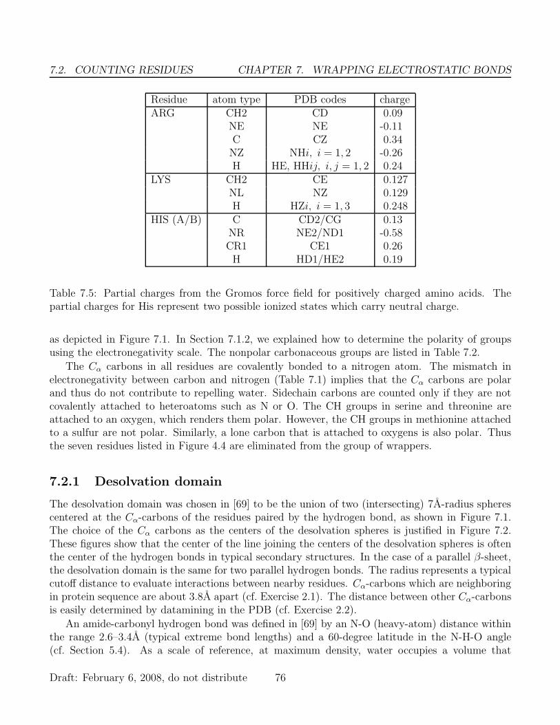
Table 7.5: Partial charges from the Gromos force field for positively charged amino acids. Thepartial charges for His represent two possible ionized states which carry neutral charge.

as depicted in Figure 7.1. In Section 7.1.2, we explained how to determine the polarity of groupsusing the electronegativity scale. The nonpolar carbonaceous groups are listed in Table 7.2.

The Cα carbons in all residues are covalently bonded to a nitrogen atom. The mismatch inelectronegativity between carbon and nitrogen (Table 7.1) implies that the Cα carbons are polarand thus do not contribute to repelling water. Sidechain carbons are counted only if they are notcovalently attached to heteroatoms such as N or O. The CH groups in serine and threonine areattached to an oxygen, which renders them polar. However, the CH groups in methionine attachedto a sulfur are not polar. Similarly, a lone carbon that is attached to oxygens is also polar. Thusthe seven residues listed in Figure 4.4 are eliminated from the group of wrappers.

7.2.1 Desolvation domain

The desolvation domain was chosen in [69] to be the union of two (intersecting) 7A-radius spherescentered at the Cα-carbons of the residues paired by the hydrogen bond, as shown in Figure 7.1.The choice of the Cα carbons as the centers of the desolvation spheres is justified in Figure 7.2.These figures show that the center of the line joining the centers of the desolvation spheres is oftenthe center of the hydrogen bonds in typical secondary structures. In the case of a parallel β-sheet,the desolvation domain is the same for two parallel hydrogen bonds. The radius represents a typicalcutoff distance to evaluate interactions between nearby residues. Cα-carbons which are neighboringin protein sequence are about 3.8A apart (cf. Exercise 2.1). The distance between other Cα-carbonsis easily determined by datamining in the PDB (cf. Exercise 2.2).

An amide-carbonyl hydrogen bond was defined in [69] by an N-O (heavy-atom) distance withinthe range 2.6–3.4A (typical extreme bond lengths) and a 60-degree latitude in the N-H-O angle(cf. Section 5.4). As a scale of reference, at maximum density, water occupies a volume that


CHAPTER 7. WRAPPING ELECTROSTATIC BONDS 7.2. COUNTING RESIDUES

O−CN−H

Figure 7.1: Caricature showing desolvation spheres with various side chains. The open circles denotethe nonpolar carbonaceous groups, and the solid circles represent the Cα carbons. The hydrogenbond between the amide (N-H) and carbonyl (O-C) groups is shown with a dashed line. Glycinesappear without anything attached to the Cα carbon. There are 22 nonpolar carbonaceous groupsin the union of the desolvation spheres and six sidechains with two or more carbonaceous groupswhose Cβ carbon lie in the spheres.

(a) (b) (c)

Figure 7.2: The hydrogen bond (dashed line) configuration in (a) α-helix, (b) antiparallel β-sheet,and (c) parallel β-sheet. A dotted line connects the Cα carbons (squares) that provide the centersof the spheres forming the desolvation domains in Figure 7.1. The amide (N-H) groups are depictedby arrow heads and the carbonyl (O-C) groups are depicted by arrow tails.


7.2. COUNTING RESIDUES CHAPTER 7. WRAPPING ELECTROSTATIC BONDS

corresponds to a cube of dimension just over 3.1A on a side (cf. Section 10.7).The average extent of desolvation, ρR, over all backbone hydrogen bonds of a monomeric struc-

ture can be computed from any set of structures. In [69], a nonredundant sample of 2811 PDB-structures was examined. The average ρR over the entire sample set was found to be 6.6 [69].For any given structure, the dispersion (standard deviation) σ from the mean value of ρR for thatstructure can be computed. The dispersion averaged over all sampled structures was found to beσ = 1.46 [69]. These statistics suggested a way to identify the extreme of the wrapping distributionas containing three or fewer wrapping residues in their desolvation domains. This can be interpretedas defining underwrapped as ρR values that are more than two standard deviations from the mean.

The distribution of the selected proteins as a function of their average wrapping as measuredby ρR is shown in Fig. 5 in [69]. The probability distribution has a distinct inflection point atρ = 6.2. Over 90% of the proteins studied have ρR > 6.2, and none of these are yet known to yieldamyloid aggregation under physiological conditions. In addition, individual sites with low wrappingon selected proteins were examined and found to correlate with known binding sites.

In Section 7.2.2, we will see that the known disease-related amyloidogenic proteins are foundin the relatively under-populated 3.5 < ρR < 6.2 range of the distribution, with the cellular prionproteins located at the extreme of the spectrum (3.5 < ρR < 3.75). We discuss there the implicationsregarding a propensity for organized aggregation. Approximately 60% of the proteins in the criticalregion 3.5 < ρR < 6.2 which are not known to be amyloidogenic are toxins whose structures arestabilized mostly by disulfide bonds.

To further assess the virtues of the residue-based assessment of wrapping, we review additionalresults and predictions of [69].

7.2.2 Predicting aggregation

Prediction of protein aggregation can be based on locating regions of the protein surface with highdensity of defects which may act as aggregation sites [104, 129, 156]. Figure 3a of [69] depicts the(many) UWHB’s for the human cellular prion protein (PDB file 1QM0) [188, 192, 246]. Over halfof the hydrogen bonds are UWHB’s, indicating that many parts of the structure must be open towater attack. For example, α-helix 1 has the highest concentration of UWHB’s, and therefore maybe prone to structural rearrangement.

In helix 1 (residues 143 to 156), all of the hydrogen bonds are UWHB’s, and this helix hasbeen identified as undergoing an α-helix to β-strand transition [188, 192, 246]. Furthermore, helix3 (residues 199 to 228) contains a significant concentration of UWHB’s at the C-terminus, a regionassumed to define the epitope for protein-X binding [188]. The remaining UWHB’s occur at thehelix-loop junctures and may contribute to flexibility required for rearrangement.

The average underwrapping of hydrogen bonds in an isolated protein may be a significant in-dicator of aggregation, but it is not likely to be sufficient to determine amyloidogenic propensity.For instance, protein L (PDB file 2PTL) is not known to aggregate even though its ρR = 5.06 valueis outside the standard range of sufficient wrapping. Similarly, trp-repressor (PDB file 2WRP)has ρR = 5.29, and the factor for inversion stimulation (PDB file 3FIS) has ρR = 4.96. Manyneurotoxins (e.g., PDB file 1CXO with ρR = 3.96) are in this range as well.


CHAPTER 7. WRAPPING ELECTROSTATIC BONDS7.3. COUNTING NONPOLAR GROUPS

The existence of short fragments endowed with fibrillogenic potential [13, 48, 57, 93, 104, 156,129] suggests a localization or concentration of amyloid-related structural defects. In view of this,a local wrapping parameter, the maximum density δmax of UWHB’s on the protein surface wasintroduced [69]. A statistical analysis involving δmax [69] established that a threshold δmax >0.38/nm2 distinguishes known disease-related amyloidogenic proteins from other proteins with alow extent of hydrogen bond wrapping. On the basis of a combined assessment, identifying bothlow average wrapping and high maximum density of underwrapping, it was predicted [69] that sixproteins might posses amyloidogenic propensity. Three of them,

• angiogenin (cf. PDB files 1B1E and 2ANG),

• meizothrombin (cf. PDB file 1A0H), and

• plasminogen (cf. PDB file 1B2I),

are involved in some form of blood clotting or wound healing, and not something related to disease.Not all protein aggregation is related to disease. Angiogenesis refers to the growth of new

capillaries from an existing capillary network, and many processes involve this, including woundhealing. Angiogenin is only one of many proteins involved in the angiogenesis process, but it appearsto have certain unique properties [136]. Meizothrombin is formed during prothrombin activation,and is known to be involved in blood clotting [119] and is able to bind to procoagulant phospholipidmembranes [182]. Plasminogen has been identified as being a significant factor in wound healing[195].

7.3 Counting nonpolar groups

A more refined measure of hydrogen-bond protection has been proposed based on the number ofvicinal nonpolar groups [65, 71]. The desolvation domain for a backbone hydrogen bond is definedagain as the union of two intersecting spheres centered at the α-carbons of the residues paired by thehydrogen bond, as depicted in Figure 7.1. In this case, all of the dark circles are counted, whetheror not the base of the sidechain lies within the desolvation domain. The extent of intramoleculardesolvation of a hydrogen bond, ρPG, is defined by the number of sidechain nonpolar groups (CHn,n = 1, 2, 3) in the desolvation domain (see Table 7.2).

The distribution of wrapping for a large sample of non-redundant proteins is given in Figure 12.1for a radius of 6A for the definition of the desolvation domain. In [72], an UWHB was defined bythe inequality ρPG < 12 for this value of the radius. Statistical inferences involving this definitionof ρPG were found to be robust to variations in the range 6.4 ± 0.6 A for the choice of desolvationradius [71, 79]. In Figure 7.3 the distribution of wrapping is presented for a particular PDB file.

7.3.1 Distribution of wrapping for an antibody complex

It is instructive to consider wrapping of hydrogen bonds from a more detailed statistical pointof view. In Figure 7.3 the distribution of wrapping is presented for the antibody complex whose


7.3. COUNTING NONPOLAR GROUPSCHAPTER 7. WRAPPING ELECTROSTATIC BONDS

0

2

4

6

8

10

12

0 5 10 15 20 25 30 35 40

frequ

ency

of o

ccur

renc

e

number of noncarbonaceous groups in each desolvation sphere: radius=6.0 Angstroms

PDB file 1P2C: Light chain, A, dotted line; Heavy chain, B, dashed line; HEL, C, solid line

line 2line 3line 4

0

2

4

6

8

10

12

0 5 10 15 20 25 30 35 40

frequ

ency

of o

ccur

renc

e

number of noncarbonaceous groups in each desolvation sphere: radius=6.0 Angstroms

PDB file 1P2C: Light chain, A, dotted line; Heavy chain, B, dashed line; HEL, C, solid line

line 2line 3line 4

Figure 7.3: Distribution of wrapping for PDB file 1P2C. There are three chains: light, heavy chainsof the antibody, and the antigen (HEL) chain. The desolvation radius is 6.0A. Smooth curves (7.2)are added as a guide to the eye.

structure is recorded PDB file 1P2C. There are three chains, two in the antibody (the light andheavy chains), and one in the antigen, hen egg-white lysozyme (HEL).

What is striking about the distributions is that they are bi-modal, and roughly comparable forall three chains. We have added a smooth curve representing the distributions

di(r) = ai|r − r0|e−|r−r0|/wi (7.2)

to interpolate the actual distributions. More precisely, d1 represents the distribution for r < r0,and d2 represents the distribution for r > r0. The coefficients chosen were w1 = 2.2 and w2 = 3.3.The amplitude coefficients were a1 = 12 and a2 = 9, and the offset r0 = 18 for both distributions.In this example, there seems to be a line of demarcation at ρ = 18 between hydrogen bonds thatare well wrapped and those that are underwrapped.

The distributions in Figure 7.3 were computed with a desolvation radius of 6.0A. Larger desol-vation radii were also used, and the distributions are qualitatively similar. However the sharp gapat ρ = 18 becomes blurred for larger values of the desolvation radius.


CHAPTER 7. WRAPPING ELECTROSTATIC BONDS7.4. RESIDUES VERSUS POLAR GROUPS

7.4 Residues versus polar groups

The two measures considered here for determining UWHB’s share some important key features.Both count sidechain indicators which fall inside of desolvation domains that are centered at the Cα

backbone carbons. The residue-based method counts the number of residues (of a restricted type)whose Cβ carbons fall inside the desolvation domain. The group-based method counts the numberof carbonaceous groups that are found inside the desolvation domain.

We observed that the average measure of wrapping based on counting residues was ρR = 6.6,whereas the average measure of wrapping based on counting non-polar groups is ρPG = 15.9.The residues in the former count represent at least two non-polar groups, so we would expectthat ρPG > 2ρR. We see that this holds, and that the excess corresponds to the fact that someresidues have three or more non-polar groups. Note that these averages were obtained with differentdesolvation radii, 6.0A for ρPG and 7.0A for ρR. Adjusting for this difference would make ρPG evenlarger, indicating an even greater discrepancy between the two measures. This implies that ρPG

provides a much finer estimation of local hydrophobicity.The structural analysis in [69] identified site mutations which might stabilize the part of the

cellular prion protein (PDB file 1QM0) believed to nucleate the cellular-to-scrapie transition. The(Met134, Asn159)-hydrogen bond has a residue wrapping factor of only ρR = 3 and is only pro-tected by Val161 and Arg136 locally, which contribute only a minimal number (five) of non-polarcarbonaceous groups. Therefore it is very sensitive to mutations that alter the large-scale contextpreventing water attack. It was postulated in [69] that a factor that triggers the prion diseaseis the stabilization of the (Met134, Asn159) β-sheet hydrogen bond by mutations that foster itsdesolvation beyond wild-type levels.

In the wild type, the only nonadjacent residue in the desolvation domain of hydrogen bond(Met134, Asn159) is Val210, thus conferring marginal stability with ρR = 3. Two of the threeknown pathogenic mutations (Val210Ile and Gln217Val) would increase the number of non-polarcarbonaceous groups wrapping the hydrogen bond (Met134, Asn159), even though the number ofwrapping residues would not change. Thus we see a clearer distinction in the wrapping environmentbased on counting non-polar carbonaceous groups instead of just residues.

The third known pathogenic mutation, Thr183Ala, may also improve the wrapping of the hy-drogen bond (Met134, Asn159) even though our simple counting method will not show this, as bothThr and Ala contribute only one nonpolar carbonaceous group for desolvation. However, Ala is fourpositions below Thr in Table 6.1 and is less polar than Thr. Table 6.1 reflects a more refined notionof wrapping for different sidechains, but we do not pursue this here.

7.5 Defining dehydrons via geometric requirements

The enhancement of backbone hydrogen-bond strength and stability depends on the partial struc-turing, immobilization or removal of surrounding water. In this section we review an attempt[73] to quantify this effect using a continuous representation of the local solvent environment sur-rounding backbone hydrogen bonds [31, 65, 71, 79, 103, 173, 230]. The aim is to estimate thechanges in the permittivity (or dielectric coefficient) of such environments and the sensitivity of


7.5. DEFINING DEHYDRONS VIA GEOMETRIC REQUIREMENTSCHAPTER 7. WRAPPING ELECTROSTATIC BONDS

the Coulomb energy to local environmental perturbations caused by protein interactions [65, 79].However, induced-fit distortions of monomeric structures are beyond the scope of these techniques.

The new ingredient is a sensitivity parameter Mk assessing the net decrease in the Coulomb en-ergy contribution of the k-th hydrogen bond which would result from an exogenous immobilization,structuring or removal of water due to the approach by a hydrophobic group. This perturbationcauses a net decrease in the permittivity of the surrounding environment which becomes more orless pronounced, depending on the pre-existing configuration of surrounding hydrophobes in themonomeric state of the protein. In general, nearby hydrophobic groups induce a structuring of thesolvent needed to create a cavity around them and the net effect of this structuring is a localizedreduction in the solvent polarizability with respect to reference bulk levels. This structuring ofthe solvent environment should be reflected in a decrease of the local dielectric coefficient ε. Thiseffect has been quantified in recent work which delineated the role of hydrophobic clustering in theenhancement of dielectric-dependent intramolecular interactions [65, 79].

We now describe an attempt to estimate ε as a function of the fixed positions rj : j = 1, . . . , nkof surrounding nonpolar hydrophobic groups (CHn, with n = 1, 2, 3, listed in Table 7.2). The simplerestimates of wrapping considered so far could fail to predict an adhesive site when it is produced byan uneven distribution of desolvators around a hydrogen bond, rather than an insufficient numberof such desolvators. Based on the fixed atomic framework for the monomeric structure, we nowidentify Coulomb energy contributions from intramolecular hydrogen bonds that are most sensitiveto local environmental perturbations by subsuming the effect of the perturbations as changes in ε.

Suppose that the carbonyl oxygen atom is at rO and that the partner hydrogen net charge is atrH . The electrostatic energy contribution ECOUL(k, r) for this hydrogen bond in a dielectric mediumwith dielectric permittivity ε(r) is approximated (see Chapter 16) by

ECOUL(r) =−1

4πε(r)

qq′

|rO − rH | , (7.3)

where q, q′ are the net charges involved and where | · | denotes the Euclidean norm.Now suppose that some agent enters in a way to alter the dielectric field, e.g., a hydrophobe

that moves toward the hydrogen bond and disrupts the water that forms the dielectric material.This movement will alter the Coulombic energy as it modifies ε, and we can use equation (7.3) todetermine an equation for the change in ε in terms of the change in ECOUL. Such a change in ECOUL

can be interpreted as a force (cf. Chapter 3). We can compute the resulting effect as a derivativewith respect to the position R of the hydrophobe:

∇R(1/ε(r)) =4π|rO − rH |

qq′(−∇RECOUL(r)) =

4π|rO − rH |qq′

F (r), (7.4)

where F (r) = −∇RECOUL(r) is a net force exerted on the hydrophobe by the fixed pre-formedhydrogen bond. This force represents a net 3-body effect [65], involving the bond, the dielectricmaterial (water) and the hydrophobe. If ECOUL is decreased in this process, the hydrophobe isattracted to the hydrogen bond because in so doing, it decreases the value of ECOUL(r).

To identify the ‘opportune spots’ for water exclusion on the surface of native structures we needto first cast the problem within the continuous approach, taking into account that 1/ε is the factor


CHAPTER 7. WRAPPING ELECTROSTATIC BONDS7.5. DEFINING DEHYDRONS VIA GEOMETRIC REQUIREMENTS

in the electrostatic energy that subsumes the influence of the environment. Thus to identify thedehydrons, we need to determine for which Coulombic contributions the exclusion or structuring ofsurrounding water due to the proximity of a hydrophobic ‘test’ group produces the most dramaticincrease in 1/ε. The quantity Mk was introduced [73] to quantify the sensitivity of the Coulombicenergy for the k-th backbone hydrogen bond to variations in the dielectric. For the k-th backbonehydrogen bond, this sensitivity is quantified as follows.

Define a desolvation domain Dk with border ∂Dk circumscribing the local environment aroundthe k-th backbone hydrogen bond, as depicted in Figure 7.1. In [73], a radius of 7A was used. Theset of vector positions of the nk hydrophobic groups surrounding the hydrogen bond is extendedfrom rj : j = 1, 2, . . . , nk to rj : j = 1, 2, . . . , nk; R by adding the test hydrophobe at positionR. Now compute the gradient ∇R(1/ε)|R=Ro , taken with respect to a perpendicular approach bythe test hydrophobe to the center of the hydrogen bond at the point R = Ro located on the circleconsisting of the intersection C of the plane perpendicular to the hydrogen bond with the boundary∂Dk of the desolvation domain. Finally, determine the number

Mk = max |∇R(1/ε)|R=Ro | : Ro ∈ C . (7.5)

The number Mk quantifies the maximum alteration in the local permittivity due to the approachof the test hydrophobe in the plane perpendicular to the hydrogen bond, centered in the middle ofthe bond, at the surface of the desolvation domain.

The quantity Mk may be interpreted in physical terms as a measure of the maximum possibleattractive force exerted on the test hydrophobic group by the pre-formed hydrogen bond. The onlydifficulty in estimating Mk is that it requires a suitable model of the dielectric permittivity ε as afunction of the geometry of surrounding hydrophobic groups. We will consider the behavior of thedielectric permittivity more carefully in Chapter 16, but for now we consider a heuristic model usedin [73].

The model in [73] for the dielectric may be written

ε−1 = (ε−1o − ε−1

w )Ω(rj)Φ(rH − rO) + ε−1w , (7.6)

where εw and εo are the permittivity coefficients of bulk water and vacuum, respectively, and

Ω(rj) =∏

j=1,...,nk

(1 + e−|rO−rj |/Λ

) (1 + e−|rH−rj |/Λ

)(7.7)

provides an estimate of the change in permittivity due to the hydrophobic effects of the carbonaceousgroups. In [73], a value of Λ = 1.8A was chosen to represent the characteristic length associated withthe water-structuring effect induced by the solvent organization around the hydrophobic groups.Further, a cut-off function

Φ(r) = (1 + |r|/ξ) e−|r|/ξ, (7.8)

where ξ = 5A is a water dipole-dipole correlation length, approximates the effect of hydrogen bondlength on its strength [73].


7.5. DEFINING DEHYDRONS VIA GEOMETRIC REQUIREMENTSCHAPTER 7. WRAPPING ELECTROSTATIC BONDS

1

1.1

1.2

1.3

1.4

1.5

1.6

1.7

1.8

0 0.5 1 1.5 2 2.5 3

line 1line 2line 3

1

1.1

1.2

1.3

1.4

1.5

1.6

1.7

1.8

0 0.5 1 1.5 2 2.5 3

line 1line 2line 3

Figure 7.4: The function ω(x, y) plotted as a function of the distance along the x-axis connecting rH

and rO, for three different values of the distance y from that axis: y = 1 (solid line), y = 2 (dashedline), y = 3 (dotted line). The coordinates have been scaled by Λ and the value of |rO − rH | = 1was assumed.

We can write the key expression Ω in (7.7) as

Ω(rj) =∏

j=1,...,nk

ω(rj), (7.9)

where the function ω is defined by

ω(r) =(1 + e−|rO−r|/Λ

) (1 + e−|rH−r|/Λ

). (7.10)

The function ω is never smaller than one, and it is maximal in the plane perpendicular to the lineconnecting rH and rO. Moreover, it is cylindrically symmetric around this axis. The values of ωare plotted in Figure 7.4 as a function of the distance from the perpendicular bissector of the axisconnecting rH and rO, for three different values of the distance y from the line connecting rH andrO.

We see that the deviation in ω provides a strong spatial dependence on the dielectric coefficientin this model. Thus hydrophobes close to the plane bissecting the line connecting rH and rO arecounted more strongly than those away from that plane, for a given distance from the axis, andthose closer to the line connecting rH and rO are counted more strongly than those further away.When the product ΦΩ = 1, we get ε = εo reflecting the maximal amount of water exclusion possible.Correspondingly, if ΦΩ = 0, ε = εw indicating a dielectric similar to bulk-water. Thus bigger valuesof Ω correspond to the effect of wrapping.

The definition (7.6) of the dielectric has not been scaled in a way that assures a limiting value ofε = εo. However, since we are only interested in comparing relative dielectric strength, this scalingis inessential. What matters is that larger values of Ω correspond to a lower dielectric and thusstronger bonds.


CHAPTER 7. WRAPPING ELECTROSTATIC BONDS 7.6. EXERCISES

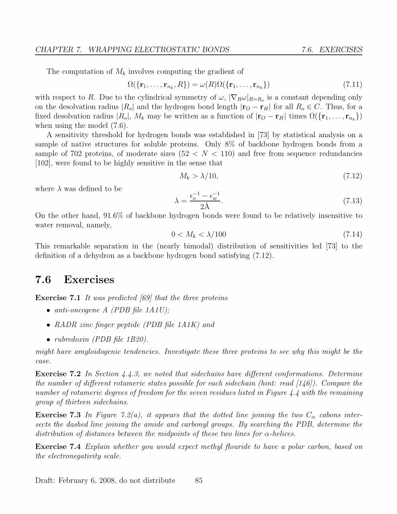
The computation of Mk involves computing the gradient of

Ω(r1, . . . , rnk, R) = ω(R)Ω(r1, . . . , rnk

) (7.11)

with respect to R. Due to the cylindrical symmetry of ω, |∇Rω|R=Ro is a constant depending onlyon the desolvation radius |Ro| and the hydrogen bond length |rO − rH | for all Ro ∈ C. Thus, for afixed desolvation radius |Ro|, Mk may be written as a function of |rO − rH | times Ω(r1, . . . , rnk

)when using the model (7.6).

A sensitivity threshold for hydrogen bonds was established in [73] by statistical analysis on asample of native structures for soluble proteins. Only 8% of backbone hydrogen bonds from asample of 702 proteins, of moderate sizes (52 < N < 110) and free from sequence redundancies[102], were found to be highly sensitive in the sense that

Mk > λ/10, (7.12)

where λ was defined to be

λ =ε−1o − ε−1

w

2A. (7.13)

On the other hand, 91.6% of backbone hydrogen bonds were found to be relatively insensitive towater removal, namely,

0 < Mk < λ/100 (7.14)

This remarkable separation in the (nearly bimodal) distribution of sensitivities led [73] to thedefinition of a dehydron as a backbone hydrogen bond satisfying (7.12).

7.6 Exercises

Exercise 7.1 It was predicted [69] that the three proteins

• anti-oncogene A (PDB file 1A1U);

• RADR zinc finger peptide (PDB file 1A1K) and

• rubredoxin (PDB file 1B20).

might have amyloidogenic tendencies. Investigate these three proteins to see why this might be thecase.

Exercise 7.2 In Section 4.4.3, we noted that sidechains have different conformations. Determinethe number of different rotameric states possible for each sidechain (hint: read [146]). Compare thenumber of rotameric degrees of freedom for the seven residues listed in Figure 4.4 with the remaininggroup of thirteen sidechains.

Exercise 7.3 In Figure 7.2(a), it appears that the dotted line joining the two Cα cabons inter-sects the dashed line joining the amide and carbonyl groups. By searching the PDB, determine thedistribution of distances between the midpoints of these two lines for α-helices.

Exercise 7.4 Explain whether you would expect methyl flouride to have a polar carbon, based onthe electronegativity scale.


7.6. EXERCISES CHAPTER 7. WRAPPING ELECTROSTATIC BONDS


Chapter 8

Stickiness of dehydrons

We have explained why under-wrapped hydrogen bonds benefit from the removal of water. Thismakes them susceptible to interaction with molecules that can replace water molecules in the vicinityof the hydrogen bond. Conceptually, this implies that under-wrapped hydrogen bonds attractentities that can dehydrate them. Thus they must be sticky. If so, it must be possible to observethis experimentally. Here we review several papers that substantiate this conclusion. One of theminvolves a mesoscopic measurement of the force associated with a dehydron [72]. A second presentsdata on the direct measurement of the dehydronic force using atomic force microscopy [63]. Anotherpaper examines the effect of such a force on a deformable surface [74].

8.1 Surface adherence force

We defined the notion of an under-wrapped hydrogen bond by a simple counting method in Chap-ter 7 and have asserted that there is a force associated with UHWB’s. Here we describe measure-ments of the adhesion of an under-wrapped hydrogen bond by analyzing the flow-rate dependenceof the adsorption uptake of soluble proteins onto a phospholipid bilayer.

8.1.1 Biological surfaces

The principal biological surface of interest is the cell membrane. This is a complex system, buta key component is what is called a phospholipid bilayer. The term lipid refers to a type ofmolecule that is a long carbonaceous polymer with a polar (phospho) group at the ‘head.’ This itis hydrophobic at one end and hydrophilic at the other. These molecules align to form a complexthat could be described as a bundle of pencils, with the hydrophilic head group (the eraser) at oneside of the surface and the hydrophobic ‘tail’ on the other side. These bundles can grow to form asurface when enough pencils are added. A second surface can form in the opposite orientation, withthe two hydrophobic surfaces in close proximity. This results in a membrane that is hydrophilic onboth sides, and thus can persist in an aqueous environment.

One might wonder what holds together a lipid bilayer. We have noted that there is a significantvolume change when a hydrophobic molecule gets removed from water contact in Section 4.4.4.


8.2. A TWO-ZONE MODEL CHAPTER 8. STICKINESS OF DEHYDRONS

The volume change causes self-assembly of lipids and provides a substantial pressure that holds thesurface together. The architecture of a lipid bilayer is extremely adaptive. For example, a curvedsurface can be formed simply by allocating more lipid to one side than the other. Moreover, iteasily allows insertion of other molecules of complex shape but with other composition. Much of acell membrane is lipid, but there are also proteins with various functions as well as other moleculessuch as cholesterol. However, a simple lipid bilayer provides a useful model biological surface.

8.1.2 Soluble proteins on a surface

One natural experiment to perform is to release soluble proteins in solution near a lipid bilayer andto see to what extent they attach to the bilayer. Such an experiment [66] indicated a significantcorrelation between the under-wrapping of hydrogen bonds and bilayer attachment. The resultswere explained by assuming that the probability of successful landing on the liquid-solid interface isproportional to the ratio of UWHB’s to all hydrogen bonds on the protein surface. Here, the numberof surface hydrogen bonds is taken simply as a measure of the surface area. Thus the ratio can bethought of as an estimate of the fraction of the surface of the protein that is under-wrapped. Theexperiments in [66] indicated that more dehydrons lead to more attachments, strongly suggestingthat dehydrons are sticky. However, such indications were only qualitative.

A more refined analysis of lipid bilayer experiments was able to quantify a force of attachment[72]. The average magnitude of the attractive force exerted by an UWHB on a surface was assessedbased on measuring the dependence of the adsorption uptake on the flow rate of the ambient fluidabove the surface. The adhesive force was measured via the decrease in attachment as the flow ratewas increased.

Six proteins were investigated in [72], as shown in Table 8.1, together with their numbers ofwell-wrapped hydrogen bonds as well as dehydrons. The UWHB’s for three of these are shown inFig. 1a-c in [72]. The particular surface was a Langmuir-Blodgett bilayer made of the lipid DLPC(1,2 dilauroyl-sn-glycero-3 phosphatidylcholine) [194]. We now review the model used in [72] tointerpret the data.

8.2 A two-zone model

In [72], a two-zone model of surface adhesion was developed. The first zone deals with the experi-mental geometry and predicts the number of proteins that are likely to reach a fluid boundary layerclose to the lipid bylayer. The probability Π of arrival is dependent on the particular experiment, sowe only summarize the model results from [72]. The second zone is the fluid boundary layer close tothe lipid bilayer, where binding can occur. In this layer, the probability P of binding is determinedby the thermal oscillations of the molecules and the solvent as well as the energy of binding.

The number M of adsorbed molecules is given by

M = ΠP (nUW , nW , T )N (8.1)

where Π is the fraction of molecules that reach the (immobile) bottom layer of the fluid, P (nUW , nW , T )is the conditional probability of a successful attachment at temperature T given that the bottom


CHAPTER 8. STICKINESS OF DEHYDRONS 8.2. A TWO-ZONE MODEL

layer has been reached, and N is the average number of protein molecules in solution in the cell.The quantities nUW and nW are the numbers of underwrapped and well-wrapped hydrogen bondson the surface of the protein, respectively. These will be used to estimate the relative amount ofprotein surface area related to dehydrons. The fraction Π depends on details of the experimentaldesign, so we focus initially on on the second term P .

8.2.1 Boundary zone model

Suppose that ∆U is the average decrease in Coulombic energy associated with the desolvation ofa dehydron upon adhesion. It is the value of ∆U that we are seeking to determine. Let ∆V bethe Coulombic energy decrease upon binding at any other site. Let f be the fraction of the surfacecovered by dehydrons. As a simplified approximation, we assume that

f ≈ nUW

nUW + nW. (8.2)

Then the probability of attachment at a dehydron is predicted by thermodynamics as

P (nUW , nW , T ) =fe∆U/kBT

(1 − f)e∆V/kBT + fe∆U/kBT≈ nUW e∆U/kBT

nWe∆V/kBT + nUW e∆U/kBT, (8.3)

with kB = Boltzmann’s constant. In [72], ∆V was assumed to be zero. In this case, (8.3) simplifiesto

P (nUW , nW , T ) =fe∆U/kBT

(1 − f) + fe∆U/kBT≈ nUWe∆U/kBT

nW + nUW e∆U/kBT(8.4)

(cf. equation (2) of [72]). Note that this probability is lower if ∆V > 0.

8.2.2 Diffusion zone model

The probability Π in (8.1) of penetrating the bottom layer of the fluid is estimated in [72] bya model for diffusion via Brownian motion in the plane orthogonal to the flow direction. Thisdepends on the solvent bulk viscosity µ, and the molecular mass, m, and the hydrodynamicradius [198] or Stokes radius [100] of the protein. This radius R associates with each protein anequivalent sphere that has approximately the same flow characteristics at low Reynolds numbers.This particular instance of a ‘spherical cow’ approximation [53, 130] is very accurate, since thevariation in flow characteristics due to shape variation is quite small [198]. The drag on a sphereof radius R, at low Reynolds numbers, is F = 6πRµv where v is the velocity. The drag is a forcethat acts on the sphere through a viscous interaction. The coefficient

ξ = 6πRµ/m = F/mv (8.5)

where m is the molecular mass, is a temporal frequency (units: inverse time) that characterizesBrownian motion of a protein. The main non-dimensional factor that appears in the model is

α =mξ2L2

2kBT=

L2(6πRµ)2/m

2kBT, (8.6)


8.3. DIRECT FORCE MEASUREMENT CHAPTER 8. STICKINESS OF DEHYDRONS

which has units of energy in numerator and denominator. We have [2]

Π(v, R, m) =

∫Λ

∫Ω\Λ

∫[0,τ ]

αL−2

πΓ(t)e−αL−2|r−r0|2/Γ(t) dtdr0dr

=

∫Λ

∫Ω\Λ

∫[0,L/v]

α

πΓ(t)e−α|r−r0|2/Γ(t) dtdr0dr

(8.7)

where r is the two-dimensional position vector representing the cell cross-section Ω, |r| denotesthe Euclidean norm of r, Λ is the 6A×108A cross-section of the bottom layer, and Γ(t) = 2ξt −3 + 4e−ξt − e−2ξt. The domains Λ and Ω represents domains scaled by the length L, and thus thevariables r and r0 are non-dimensional. In particular, the length of Λ and Ω is one in the horizontalcoordinate. Note that Γ(t) = 2

3(ξt)3 + O((ξt)4) for ξt small. Also, since the mass m of a protein

tends to grow with the radius cubed, α actually decreases like 1/R as the Stokes radius increases.

8.2.3 Model validity

The validity of the model represented by equations (8.1—8.7) was established by data fitting. Theonly parameter in the model, ∆U , was varied, and a value was found that consistently fits withinthe confidence band for the adsorption data for the six proteins (see Fig. 3 of [72]) across the entirerange of flow velocities v. This value is

∆U = 3.91 ± 0.67 kJ/mole = ∆U = 0.934 ± 0.16 kcal/mole. (8.8)

This value is within the range of energies associated with typical hydrogen bonds. Thus we canthink of a dehydron as a hydrogen bond that gets turned ‘on’ by the removal of water due to thebinding of a ligand.

Using the estimate (8.8) of the binding energy for a dehydron, an estimate was made [72] of theforce

|F | = 7.78 ± 1.5pN (8.9)

exerted by the surface on a single protein molecule at a 6A distance from the dehydron.

8.3 Direct force measurement

The experimental techniques reviewed in the previous section suggest that the density of dehydronscorrelates with protein stickiness. However, the techniques are based on measuring the aggregatebehavior of a large number of proteins. One might ask for more targeted experiments seeking toisolate the force of a dehydron, or at least a small group of dehydrons. Such experiments werereported in [63] based on atomic force microscopy (AFM).

We will not give the details of the experimental setup, but just describe the main points. Themain concept was to attach hydrophobic groups to the tip of an atomic force microscope. Thesewere then lowered onto a surface capable of forming arrays of dehydrons. This surface was formed by


CHAPTER 8. STICKINESS OF DEHYDRONS 8.3. DIRECT FORCE MEASUREMENT

protein name PDB code residues WWHB dehydronsapolipoprotein A-I 1AV1 201 121 66β lactoglobulin 1BEB 150 106 3

hen egg-white lysozyme 133L 130 34 13human apomyoglobin 2HBC 146 34 3

monomeric human insulin 6INS 50 30 14human β2-microglobulin 1I4F 100 17 9

Table 8.1: Six proteins and their hydrogen bond distributions. WWHB=well-wrapped hydrogenbonds.

a self-assembling monolayer of the molecules SH-(CH2)11-OH. The OH “head” groups are capableof making OH-OH hydrogen bonds, but these will be exposed to solvent and not well protected.

The data obtained by lowering a hydrophobic probe on such a monolayer are complex to inter-pret. However, they become easier when they are compared with a similar monolayer not containingdehydrons. In [63], the molecule SH-(CH2)11-Cl was chosen.

The force-displacement curve provided by the AFM have similarities for both monolayers [63].For large displacements, there is no force, and for very small displacements the force grows sub-stantially as the tip is driven into the monolayer. However, in between, the characteristics are quitedifferent.

For the OH-headed monolayer, as the displacement is decreased to the point where the hy-drophobic group on the tip begins to interact with the monolayer, the force on the tip decreases,indicating a force of attraction. Near the same point of displacement, the force on the tip increasesfor the chlorine-headed monolayer. Thus we see the action of the dehydronic force in attracting thehydrophobes to the dehydron-rich OH-headed layer. On the other hand, there is a resistance at thesimilar displacement as the hydrophobic tip begins to dehydrate the chlorine-headed monolayer.Ultimately, the force of resistance reaches a maximum, and then the force actually decreases to aslightly negative (attractive) value as the monolayer becomes fully dehydrated. It is significant thatthe displacement for the force minimum is approximately the same for both monolayers, indicatingthat they both correspond to a fully dehydrated state.

The force-displacement curves when the tip is removed from the surface also provide importantdata on the dehydronic force. The force is negative for rather large displacements, indicatingthe delay due to the requirements of rehydration. Breaking the hydrophobic bond formed by thehydrophobic groups on the tip and the monolayer requires enough force to be accumulated tocompletely rehydrate the monlayer. This effect is similar to the force that is required to removesticky tape, in which one must reintroduce air between the tape and the surface to which it wasattached. For the chlorine-headed monolayer, there is little change in force as the displacementis increased by four Angstroms from the point where the force is minimal. Once the threshold isreached then the force returns abruptly to zero, over a distance of about one Angstrom. For theOH-headed monolayer, the threshold is delayed by another two Angstroms, indicating the additionaleffect of the dehydronic force.


8.4. MEMBRANE MORPHOLOGY CHAPTER 8. STICKINESS OF DEHYDRONS

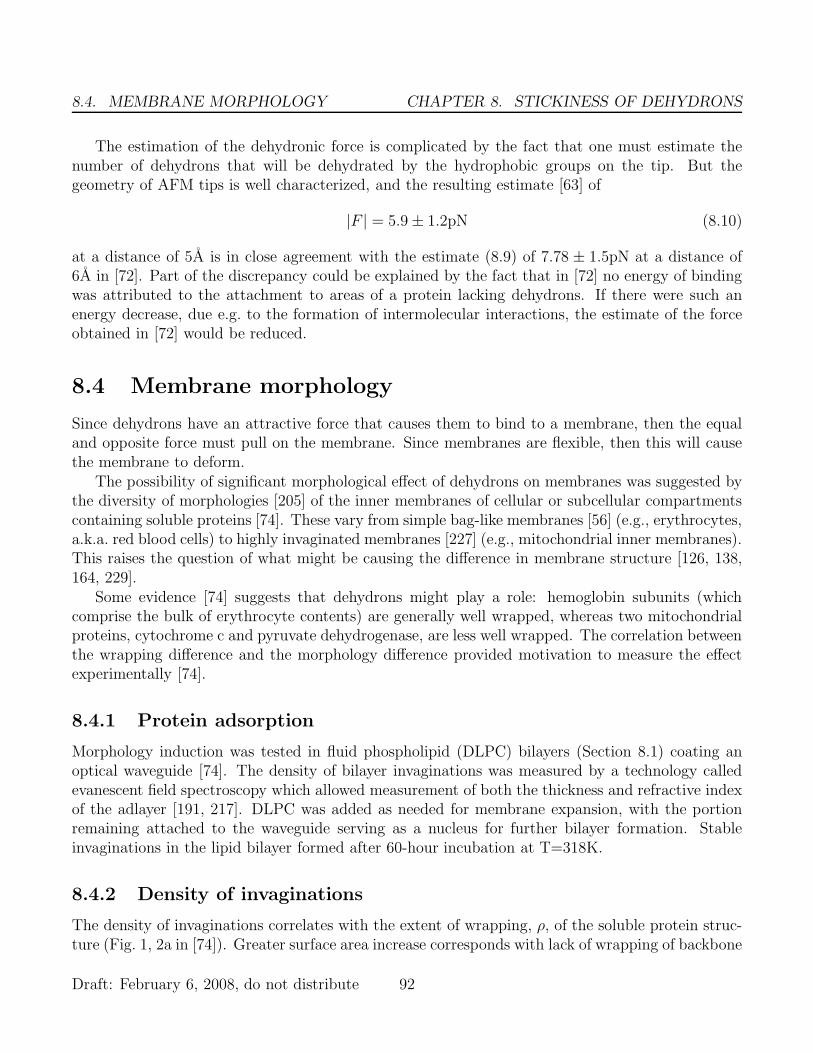
The estimation of the dehydronic force is complicated by the fact that one must estimate thenumber of dehydrons that will be dehydrated by the hydrophobic groups on the tip. But thegeometry of AFM tips is well characterized, and the resulting estimate [63] of

|F | = 5.9 ± 1.2pN (8.10)

at a distance of 5A is in close agreement with the estimate (8.9) of 7.78 ± 1.5pN at a distance of6A in [72]. Part of the discrepancy could be explained by the fact that in [72] no energy of bindingwas attributed to the attachment to areas of a protein lacking dehydrons. If there were such anenergy decrease, due e.g. to the formation of intermolecular interactions, the estimate of the forceobtained in [72] would be reduced.

8.4 Membrane morphology

Since dehydrons have an attractive force that causes them to bind to a membrane, then the equaland opposite force must pull on the membrane. Since membranes are flexible, then this will causethe membrane to deform.

The possibility of significant morphological effect of dehydrons on membranes was suggested bythe diversity of morphologies [205] of the inner membranes of cellular or subcellular compartmentscontaining soluble proteins [74]. These vary from simple bag-like membranes [56] (e.g., erythrocytes,a.k.a. red blood cells) to highly invaginated membranes [227] (e.g., mitochondrial inner membranes).This raises the question of what might be causing the difference in membrane structure [126, 138,164, 229].

Some evidence [74] suggests that dehydrons might play a role: hemoglobin subunits (whichcomprise the bulk of erythrocyte contents) are generally well wrapped, whereas two mitochondrialproteins, cytochrome c and pyruvate dehydrogenase, are less well wrapped. The correlation betweenthe wrapping difference and the morphology difference provided motivation to measure the effectexperimentally [74].

8.4.1 Protein adsorption

Morphology induction was tested in fluid phospholipid (DLPC) bilayers (Section 8.1) coating anoptical waveguide [74]. The density of bilayer invaginations was measured by a technology calledevanescent field spectroscopy which allowed measurement of both the thickness and refractive indexof the adlayer [191, 217]. DLPC was added as needed for membrane expansion, with the portionremaining attached to the waveguide serving as a nucleus for further bilayer formation. Stableinvaginations in the lipid bilayer formed after 60-hour incubation at T=318K.

8.4.2 Density of invaginations

The density of invaginations correlates with the extent of wrapping, ρ, of the soluble protein struc-ture (Fig. 1, 2a in [74]). Greater surface area increase corresponds with lack of wrapping of backbone


CHAPTER 8. STICKINESS OF DEHYDRONS 8.5. KINETIC MODEL OF MORPHOLOGY

hydrogen bonds. The density of invaginations as a function of concentration (Figure 2b in [74])shows that protein aggregation is a competing effect in the protection of solvent-exposed hydrogenbonds ([71, 65, 66, 60, 79]): for each protein there appears to be a concentration limit beyond whichaggregation becomes more dominant.

8.5 Kinetic model of morphology

The kinetics of morphology development suggest a simple morphological instability similar to thedevelopment of moguls on a steep ski run. When proteins attach to the surface, there is a forcethat binds the protein to the surface. This force pulls upward on the surface (and downward on theprotein) and will increase the curvature in proportion to the local density of proteins adsorbed onthe surface [66]. The rate of change of curvature ∂g

∂t is an increasing function of the force f :

∂g

∂t= φ(f) (8.11)

for some increasing function φ. Note that

φ(0) = 0; (8.12)

if there is no force, there will be no change. The function φ represents a material property of thesurface.

The probability p of further attachment increases as a function of the curvature at that pointsince there is more area for attachment where the curvature is higher. That is, p(g) is also anincreasing function.

Of course, attachment also reduces surface area, but we assume this effect is small initially.However, as attachment grows, this neglected term leads to a ‘saturation’ effect. There is a pointat which further reduction of surface area becomes the dominating effect, quenching further growthin curvature. But for the moment, we want to capture the initial growth of curvature in a simplemodel. We leave as Exercise 8.2 the development of a more complete model.

Assuming equilibrium is attained rapidly, we can assert that the force f is proportional to p(g):f = cp(g) at least up to some saturation limit, which we discuss subsequently. If we wish to beconservative, we can assert only that

f = ψ(p(g)) (8.13)

with ψ increasing. In any case, we conclude that f may be regarded as an increasing function ofthe curvature g, say

f = F (g) := φ(ψ(p(g))). (8.14)

To normalize forces, we should have no force for a flat surface. That is, we should assume thatp(0) = 0. This implies, together with the condition φ(0) = 0, that

F (0) = 0. (8.15)


8.6. EXERCISES CHAPTER 8. STICKINESS OF DEHYDRONS

The greater attachment that occurs locally causes the force to be higher there and thus thecurvature to increase even more, creating an exponential runaway (Fig. 4 in [74]). The repeatedinteractions of these two reinforcing effects causes the curvature to increase in an autocatalyticmanner until some other process forces it to stabilize.

The description above can be captured in a semiempirical differential equation for the curvatureg at a fixed point on the bilayer. It takes the form

∂g

∂t= F (g), (8.16)

where F is the function in (8.14) that quantifies the relationships between curvature, probability ofattachment and local density of protein described in the previous paragraph. Abstractly, we knowthat F is increasing because it is the composition of increasing functions. Hence F has a positiveslope s at g = 0. Moreover, it is plausible that F (0) = 0 using our assumptions made previously.

Thus the curvature should grow exponentially at first with rate s. In the initial stages of interfacedevelopment, F may be linearly approximated by virtue of the mean value theorem, yielding theautocatalytic equation:

∂g

∂t= sg. (8.17)

Figure 4 in [74] indicates that the number of invaginations appears to grow exponentially at first,and then saturates.

We have observed that there is a maximum amount of protein that can be utilized to cause mor-phology (Figure 2b in [74]) beyond which aggregation becomes a significantly competitive process.Thus, a ‘crowding problem’ at the surface causes the curvature to stop increasing once the numberof adsorbed proteins gets too high at a location of high curvature.

8.6 Exercises

Exercise 8.1 Determine the minimal distance between a hydrophobe and a backbone hydrogen bondin protein structures. That is, determine the number of wrappers as a function of the desolvationradius, and determine when, on average, this tends to zero.

Exercise 8.2 Derive a more refined model of morphological instability accounting for the reductionof surface area upon binding. Give properties of a function F as in (8.14) that incorporate the effectof decreasing surface area, and show how it would lead to a model like (8.16) which would saturate(rather than grow exponentially forever), reflecting the crowding effect of the molecules on the lipidsurface.


c h a p ter 7 w ra p p in g electro sta tic b o n d...

Documents