cahier de recherche 2009-06 - uqam(2007), chap.11. as said by l'habitant (2004), the kalman is...

1

Cahier de recherche

2009-06

Modeling Hedge Fund Returns Using the Kalman Filter: An Errors-in-Variables Perspective

François-Éric Racicot†

Raymond Théoret††

(IAES, October 2009)

†Professor of finance, Department of administrative sciences, University of Quebec - Outaouais (UQO), 101, St-John-Bosco Street, Lucien-Brault Building, Gatineau (Hull), Quebec, Canada, J8X 3X7. E-mail: [email protected], Tel. number: (819) 595-3900 ext. 1727. ††Professor of finance, Department of finance, University of Quebec - Montreal (UQAM), 315 Ste-Catherine east, Montreal, Quebec, Canada. H3X 2X2. E-mail: [email protected]. Tel. number: (514) 987-3000 ext. 4417.

2

Modeling Hedge Fund Returns Using the Kalman Filter: An Errors-in-Variables Perspective

Abstract

Many studies on Hedge fund returns are static, resorting frequently to a multifactor model composed of mimicking portfolios or benchmarks that account for the style of the different strategies followed by hedge funds. Yet hedge fund strategies are essentially dynamic. As conditional models appear promising to explain the dynamic strategies of portfolio managers, we study in this article how the portfolio manager alphas and betas react to financial market variables, market risk premium, interest rate, market volatility and business cycles. In this paper, we thus propose an innovative application of the Kalman Filter to dynamize these important risk factors and to account for measurement errors which create bias in the estimation process of these important parameters. Keywords: Hedge funds; Dynamic strategies; Kalman filter; Market models; Beta cycles. JEL classification: c13;c22;c51; g12;g23.

Modélisation des rendements des fonds de couverture et filtre de Kalman : Une approche basée sur les erreurs de mesure

Résumé

La majorité des études sur le comportement des rendements des fonds de couverture sont formulées dans un cadre d’analyse statique et recourent fréquemment à des modèles multifactoriels composés de portefeuilles dupliquants ou de portefeuilles de référence qui prennent en compte le style des différentes stratégies suivies par les fonds de couverture. Toutefois les stratégies des fonds de couverture sont essentiellement dynamiques. Puisque les modèles conditionnels s’avèrent prometteurs pour expliquer les stratégies dynamiques des gestionnaires de portefeuille, nous étudions dans cet article l’influence sur le sentier temporel des alphas et des bêtas des gestionnaires des variables suivantes : prime de risque du marché, taux d’intérêt, volatilité des marchés et cycle d’affaires. Dans cet article, nous proposons une approche novatrice du filtre de Kalman qui cherche à dynamiser les facteurs de risque importants tout en tenant compte des erreurs de mesure qui pourraient créer un biais d’estimation au niveau des paramètres alpha et bêta.

Mots-clefs: Fonds de couverture; Stratégies dynamiques; Filtre de Kalman; Modèles de marché; Cycles du bêta. Classification JEL: c13;c22;c51; g12;g23.

3

Introduction

Many studies on hedge fund returns are static, resorting frequently to a multifactor model

composed of mimicking portfolios or benchmarks which account for the style of the different

strategies followed by hedge funds. While classical linear regressions constitute a

parsimonious approach to the modeling of hedge fund strategies, time-invariant factor

loadings might be misleading (Berkelaar et al., 2009). Hedge fund strategies are essentially

dynamic. As conditional models appear promising to explain the dynamic strategies of

portfolio managers, we study in this paper how the portfolio manager alphas and betas react to

financial market variables like market risk premium, interest rate or market volatility or

macroeconomic variables like the business cycle.

Ferson and Schadt (1996), Christopherson, Ferson and Glassman (1998) and Ferson and

Qian (2004) had proposed a least-squares procedure to make conditional the alpha and the

beta, especially in the framework of the CAPM or the Fama and French model. These authors

were preoccupied by the high level of the alpha shown by some portfolio strategies and

particularly hedge fund strategies. They wanted to see if some conditioning variables would

not bring the unconditional alpha closer to 0, in which case the market efficiency criterion

would not be disproved.

The difficulty with these procedures is that they are estimated by a least-squares process,

which is not a dynamic but a static algorithm. They thus contain some part of arbitrariness

because we can obtain quite different results for the unconditional alpha and beta by simply

changing the conditioning information1. It seems preferable to resort to a dynamic algorithm

which recomputes the conditional alpha and beta at every period, according to the flow of last

news.

1 On that matter see: Coën, Racicot and Théoret (2006a and 2006b) and Racicot and Théoret (2006b), Coën and Racicot (2007), Racicot and Théoret (2007, 2008a, 2009) and Gregoriou (2009).

4

Using the Kalman filter procedure seems very promising to compute optimally the

conditional alpha and beta but there are few hedge fund studies resorting to this approach.

L'Habitant (2004) report that the only the study of Swinkels and van der Sluis (2001) on that

matter. In their paper, the conditional alpha and beta follow a pure random walk (recursive)

process. A subsequent paper of Bollen and Whaley (2006), which also aims to model the

expectation of hedge fund returns by the Kalman filter, viewed also the conditional alpha and

beta as a random walk process. Some authors (Swinkels & Van Der, 2006) propose to use

rather than rolling regression, as it cannot properly account for time-varying betas and since

the selected window is ad hoc, to use the Kalman filter for the mutual funds for running

return-based-style analysis to estimate factor exposure. More recently, Mamaysky et al.

(2007, 2008) also propose using the Kalman filter to evaluate the performance of mutual

funds with time-varying parameters. As explained by Berkelaar et al. 2009, the fact that the

classical regression models are by nature static and thus lead to misleading results is a

weakness of the standard approach in the context of hedge returns analysis, precisely one

weakness that the Kalman Filter aims to solve. Another quality of the Kalman Filter much

less discussed in the finance literature, is the duality relating this algorithm to the Bellman

equation (Ljungqvist & Sargent, 2004), that is essentially an algorithm for computing

conditional expectations (optimal linear projections). This, in turn, gives it a formal ground

which is much needed in finance since most models used in that field are purely ad hoc

(Cochrane 2005). That is, the estimated equation are not based or obtained from a constrained

optimization problem. This could be considered as an improvement with respect to the

scientific rigor, which is not mainstream in the practice of most financial applications (e.g.

like the Fama & French model, most option pricing models used in practice are derived

assuming a non-arbitrage framework or a partial equilibrium, not a general equilibrium). The

Kalman Filter can also be generalized further to non-linear State-Space framework by

5

assuming a hidden Markov model for the state process. That, in turn, is another very

important advantage of this algorithm which shows its flexibility and might be very useful to

operationalize more complex nonlinear financial models used in practice.

An interesting subject which some authors have studied and deserving to be studied here

(Swinkels and van der Sluis, 2001 and Bollen and Whaley, 2006) is the assumption that the

important parameters, i.e. the conditional alpha and beta, follow a random walk. Those

parameters might in fact not follow a pure random walk process, but instead the conditional

alpha and beta may also react to conditioning financial market or macroeconomic

information2. That is why we explore in this study, in a Kalman filter framework, the reaction

of conditional alpha and beta of HFR hedge funds indices classified by strategies to financial

market variables, which are in this article the interest rate variable, the market risk premium

and the squared market risk premium. Our results show that the alphas of the majority of the

indices are not very responsive to financial market variables, except for very specific

strategies. A pure recursive process seems therefore preferable for the alpha. The data

generating process of the alpha is thus more akin to a random walk process than to a

conditional model, a result in line with the market efficiency hypothesis. The alpha thus does

not appear very manageable. On the contrary, the conditional beta is much more responsive to

market conditions and it seems therefore much more manageable than the alpha. The

estimated beta follows a cycle related to financial markets conditions. Finally, we also

propose a possible extension of our dynamic model for the presence of measurement errors.

To do so, we rely on our previous contribution (Racicot & Théoret, 2008a, 2009 or Coën &

Racicot, 2007) on that matter and suggest a theoretically viable solution using the augmented

Hausman artificial regression with time-varying coefficients.

2 Actually, the conditional alpha and beta may respond to many economic and financial news, but we limit ourselves in this paper to financial market variables because a model resorting to the Kalman filter as its estimation process ought to be parsimonious. If not, the estimated coefficients will not be significant.

6

The structure of this paper is as follows. Section 2 presents the three conditional models

tested in this study, which are all built in a Kalman filter framework. We conclude that section

with our proposed solution for the problem of errors-in-variables in the setting of the Kalman

Filter. Section 3 provides an analysis of our results. Section 4 concludes.

1. Conditional model of the hedge fund returns.

A Kalman filter model is usually made up of an observation or measurement equation and

of state or transition equations for the unobserved variables or coefficients3. To explain the

expected hedge fund excess returns, we choose, as measurement equation, the three factor

Fama and French (1992, 1993 and 1997) model:

( ) tttftmtttftpt HMLSMBRRRR εβββα +++−+=− 321 (1)

with: ftpt RR − : the excess return of a portfolio, Rft being the risk-free return;

ftmt RR − : the market risk premium;

SMB: a portfolio which mimics the “small firm anomaly”, which is long in the

returns of selected small firms and short in the returns of selected big firms;

HML: a portfolio which mimics the “income stock anomaly”, which is long in

returns of stocks of selected firms having a high (book value/ market value)

ratio (value stocks) and short in selected stocks having a low (book value/

market value) ratio (growth stocks);

αt: the conditional alpha;

3 For an introduction to the Kalman filter and its uses in finance, see: Rachev et al. (2007), chap.11. As said by L'Habitant (2004), the Kalman is like a least squares estimation except that the coefficients of the model are updated at every period following the advent of new information. The applications of the Kalman filter in finance might be found in papers related to asset pricing, term structure models and in corporate finance to forecast important ratios like the price-earning ratio [Racicot and Théoret, 2006a, chap. 21]. The applications of the Kalman filter in finance go back to the beginning of the eighties. At this time, the filter was used to forecast the real rate of interest and the risk premia in forward and futures markets [Fama and Gibbons, 1982; Hsieh and Kulatilaka, 1982]. Bassett, France & Pliska [1991] resorted to the Kalman filter to forecast forward prices of nontrading securities. There are also extensive applications in the fields of exchange rates and term structure of interest rates where the Kalman filter is used to forecast volatility and other key variables [Wolff, 1987; Pennacchi, 1991]. Finally, there are nevertheless few studies in the hedge fund area to analyse their style dynamics, especially the time varying dimensions of alpha and beta [Swinkels and Van der Sluis, 2001].

7

β1t: the conditional beta;

εt: the innovation of the equation.

To explain the excess return of a portfolio, Fama and French added to the CAPM

market risk premium two other risk factors: the SMB and HML ones. We omitted in this

equation the momentum factor proposed by Jegadesh and Titman (1993) and Carhart

(1997) because the influence of this factor is weak for the majority of hedge funds, a

Kalman Filter representation of a process having to be parsimonious4.

According to Capocci and Hübner (2004), a positive sign for SMB in equation (1)

would indicate that a portfolio manager, here a hedge fund, prefers the stocks of small

firms over the stocks of larger ones, what is usually the case for hedge funds. Moreover, a

positive sign for the variable HML would be symptomatic of a preference for stocks with

a high book-to-market value ratio over stocks with a low book-to-market value ratio,

what is also a frequent preference in the hedge fund industry5.

The transition equations give the representation of the conditional alpha (αt) and

beta (β1t). We formulate three models for these conditional parameters, labelled

respectively model 1, 2 and 3.

2.1 Model 1: pure recursive model

Model 1 is a purely recursive representation of the conditional coefficients of

equation (1). Their respective equation is therefore:

4 While the Fama & French model is still a popular choice to model hedge fund returns, other more parsimonious models have appeared recently in the literature, for instance Berkelaar et al. (2009). These authors suggest that hedge fund strategies could be modeled using the following parsimonious equation:

tFI

thFI

thEQ

thEQ

ththth rrr εββα +++= ,,,,,, . This simple two-factor model uses the returns on equity (rEQ) and those on fixed income (rFI) securities, as many studies have shown that a significant portion of hedge fund return strategies are well explained by these two factors. The parameter th,α represents the time-varying alpha of strategy h and the other components represent the systematic beta components. Thus, the performance at every time period of a particular strategy can be explained by the manager skills (alpha), the returns on equity (stocks) and the returns on fixed income securities (e.g. bonds). Because of the time-varying nature of their model, they rely on the Kalman Filter to estimate the model parameters. 5 The signs of the factor loadings are seldom discussed in the studies of the F&F model. This gap must be filled because the signification of these signs is partly a matter of interpretation.

8

ttt ξαα += −1 (2)

tt,t νββ += −111 (3)

with ξt and νt being respectively the innovations terms of equations (2) and (3). If

),(iid~t 10ξ and ),(iid~t 10ν 6 equations (2) and (3) would amount to pure random walk

processes. We do not impose such constraints here. We let the filter find by its own way

the optimal recursive process.

The filtering of the conditional coefficients in the framework of a pure recursive

process is easy to understand. For instance, in equation (3), the coefficient estimated a

period t-1 serves as a seed value (a guess) for the estimation of the coefficient at time t.

But the filtered coefficient at time t is computed optimally by the Kalman filter in regard

of the flow of new information which accumulates from one period to the other.

Therefore the estimated coefficient tˆ

1β may be quite different from the coefficient

estimated one period earlier, that is 1,1 −tβ .

2.2 Model 2: recursive model combined with conditioning financial market variables Model 2 views the filtered conditional variables as a recursive process combined

with two variables representing financial market conditions: the level of interest rate and

the market risk premium. These variables will allow following the reaction of the

conditional coefficients to the conditioning market information. In this model, the filtered

conditional alpha and beta are thus:

ttttt mktr ξϕϕαα +++= −−− 12111 (4)

tttt,t mktr νϕϕββ +++= −−− 1413111 (5)

with r, the level of interest rate, and mkt, the market risk premium, that is the spread

between the return of the market portfolio and the risk-free return. The conditioning

6 In these cases, the innovations are white noise.

9

variables are lagged on period, our aim being to follow the reaction of the conditional

coefficients to the conditioning market information. The retained financial variables are

thus known at time t.

Notice that equation (4), like equation (5), might be written in first differences. For

instance, equation (4) might be written as:

( ) ttttt mktr ξϕϕαα ++=− −−− 12111 . (4')

That means that the revision of the conditional alpha from one period to the other is

function of three elements: the interest rate observed one period earlier, the market risk

premium also observed one period earlier and an error. The coefficients φ1, φ2 and the

error term result from the searching process of the filter.

We can pause a little to specify the expected sign of the variables incorporated in

equations (4) and (5). An increase in the interest rate might be perceived as good news or

bad news by hedge funds. If this increase is seen as a forthcoming deterioration of the

stock market trend or as an indicator of inflation, that is bad news. But for hedge funds

which follow call-like strategies, that might be good news. The signs of φ1 and φ3 are thus

indeterminate in equations (4) and (5). As we will see in the empirical section of this

paper, this sign is related to the specific hedge fund strategies.

In equation (4), an increase in the market risk premium at time t-1, that is an

indication of a market strengthening, may incite hedge funds to position themselves for

an increase in their alpha, this positioning being dependent on the portfolio manager

skills. In this case, the sign of 2ϕ would be positive. But if the alpha is not manageable,

this coefficient will not be different from 0. It is postulated in this paper that the alpha is

not generally manageable. Therefore, we expect that the conditioning variables would not

be significant in the equation (4): the conditional alpha is thus seen purely recursive.

10

But that is not the case for the conditional beta which is viewed as a control

variable. If the market risk premium obeys to a martingale process, we can write:

( ) 1−=Ω ttt mkt/mktE (6)

with Ωt being the information set.

According to equation (6), and increase of the market risk premium a time t-1 is

viewed as a strengthening of the stock market. That should encourage hedge funds to take

more risk and therefore to increase their beta. The sign of 4ϕ would thus be positive in

equation (5). However, Ferson and Schadt (1996) observed what seems to be a beta

puzzle in the mutual fund industry, that is a negative link between their beta and the

market risk premium. This behaviour seemed perverse to them. Our study will allow

seeing if there is such a beta puzzle in the hedge fund industry.

2.3 Model 3: model 2 plus the squared market risk premium

Model 3 is written as such:

tttttt mktmktr ξϕϕϕαα ++++= −−−−2

1512111 (7)

ttttt,t mktmktr νϕϕϕββ ++++= −−−−2

161413111 (8)

We thus introduced in the equations (4) and (5) of the conditional alpha and beta the

square of the market risk premium as an indicator of stock market volatility, that is the

second moment of the market risk premium7. An increase of market volatility should

usually induce hedge funds to bear less risk, and therefore to decrease their beta, but it

remains that an increase in market volatility might be welcomed by some hedge fund

strategies whose hedging activities are particularly important. Nevertheless, according to

Treynor and Mazuy (1966), the squared market risk premium might serve to detect good or

7 That is to say that the market volatility is another factor which contributes to the revision of the conditional alpha and beta from one period to the other.

11

bad market timing8, a good market timing being associated to a positive sign for this

variable. The sign of the squared market risk premium is thus theoretically indeterminate in

equation (8).

It is difficult to determine a priori the sign of 5ϕ in equation (7). Perhaps the

opportunities for stock selectivity are enhanced in a more volatile market. In this

perspective, the sign of 5ϕ would be positive. But, as said before, if the alpha is not

manageable, the impact of this variable would be near zero like for the other market

variables appearing in the equation of the conditional alpha.

2.4 Errors-in-Variables and the Kalman Filter

Another aspect of the modeling of hedge fund returns that have not been much studied yet

in the empirical literature is the behaviour of the Kalman Filter in the context of errors in the

explanatory variables. Here our goal is to propose a theoretical model for handling this kind

of problems (errors-in-variables and other kinds of specification errors) but we leave the

interesting subject of how to empirically implement this new approach to further research.

As shown in Coën & Racicot (2007) and Racicot & Théoret (2008a, 2009), it is quite

easy theoretically speaking to account for errors in the explanatory variables. One must

transform a regression model into an artificial Hausman regression one. In our particular

case, our basic model could be extended to include the problem of errors-in-variables as

ttttttftmtttftpt ewwwHMLSMBrrrr ++++++−+=− 332211321 ˆˆˆ)( ϕϕϕβββα (9)

where the time-varying parameters could be defined initially, for parsimony, in their simplest

form, which is a standard random walk process

ttt v11 += −αα (10)

ttt v2111 += −ββ (11)

8 In this situation, the squared market risk premium represents the co-asymetry of a given portfolio return with the market return.

12

In equation (9) the variables itw , i=1,..,3, are included to account for the potential correlation

between the explanatory variables and the error term te . We compute these elements as

follows

xxw ˆˆ −= (12)

where x is the matrix of the explanatory variables expressed in deviation from its mean, and

xZZZZx ')'(ˆ 1−= (13)

where Z is a matrix instrumental variables which use as instruments the cumulants or the

higher moments of order two and three of the explanatory variables. To operationalyze the

computation of this procedure, we use a computer code which runs in EViews and developed

by the authors whose formulation can be found in Racicot & Théoret (2008a, 2008b). As

explained previously, the time-varying coefficients can also be explained by some factors.

This means that the basic random walk model, which constrains the time-varying coefficients

to behave in a purely recursive fashion, can be generalized further to include some

explanatory components, as shown in equations (7) and (8). We leave these and other

potential generalizations of that model for future work.

2. Empirical results

3.1 The data

This study is based on a sample of the HFR indices. Statistical information on this

sample appears in table 1. Our observation period of the monthly returns of these hedge

fund indices runs from January 1997 to December 2005, for a total of 108 observations.

The risk factors which appear in the F&F equation, -that is the market risk premium and

the two mimicking portfolios: SMB and HML -, are for their part drawn from the French’s

13

website9. The interest rate used to test the models is the American three months Treasury

bill rate and the chosen market portfolio index is the S&P500.

Table 1 gives the descriptive statistics of the HFR retained indices over the period

1997-2005. This period was plagued by three major financial crises: i) the Asian financial

crisis (1997); ii) the Russian/LTCM10 crisis (1998); iii) the bursting of the high-tech market

bubble (2000). Our period of analysis is therefore rich in major stock market corrections. In

spite of these market collapses, table 1 reveals that the HFR hedge funds performed very well

during this period. The mean monthly return of these indices was 0.88% over this period, for

an annual rate of 10.6%. That rate is higher than the annual mean return of the S&P500 over

the same period, which was 8.6%. The low performers over this period were the short sellers

and the equity market neutral indices whereas the high performers were the emerging

markets, the equity hedge and non hedge indices.

Moreover, the standard deviation of the returns differs greatly from one index to the

other. The standard deviation of the returns of the indices are generally below the one of the

S&P500 index except for the short seller index which incidentally has the lowest mean return

over the period of analysis. As expected, the equity market neutral index has the lowest

standard deviation but it still performed relatively well in spite of its low volatility.

Several researchers argue that the strategies followed by hedge funds are similar to

option-based strategies. And effectively, table 1 reveals that hedge fund strategies are actually

similar to hedged option strategies, like the covered call and protective put ones. Similarly to

the hedge fund indices, these option-based strategies have a beta which is quite low, of the

order of 0.6 for at-the money options, and may yet offer all the same quite high returns which

9 The address of the French’s website is : http://mba.tuck.dartmouth.edu/pages/faculty/ken.french/data_library.html. 10 LTCM is the acronym of Long Term Capital Management, a highly levered American hedge fund which sustained massive losses in 1998.

14

approximate those shown in table 111. Furthermore, the non-hedged option-based strategies

might give a mean return which is much higher than those ones of table 1 but at the cost of a

much higher beta in the order of 7. For instance, a plain vanilla call which is at-the-money

might have a beta equal to 8.

Please insert table 1 here

Plain vanilla puts have a negative expected return. That might explain the low mean

return of the short seller index over the period of analysis. Incidentally, the CAPM beta of the

short seller index, equal to -1.22, is negative and quite high in absolute value over the period

of analysis. According to the CAPM, the excess return of a portfolio having a negative beta

should be low and even negative and that is the case of the short seller index. Another index

which has a very low beta on table 1 is the equity market neutral index and its mean return is

among the lowest in conformity with the CAPM.

Furthermore, according to table 1, the composite index of hedge funds has more

kurtosis than the market one, a characteristic shared by almost every hedge fund strategy. A

high kurtosis means that rare or extreme events are more frequent than in a normal

distribution and that nonlinearities of payoffs are very present. Once more, we may relate

these statistics to those associated to the cash-flows of option-based strategies. They have a

relatively low standard deviation but a high degree of kurtosis in comparison with the returns

of the market index.

3.2 The results

In this section, we will consider sequentially the estimation of the three models presented

in section 2.

11 For a discussion of the beta and the mean return of option-based strategies, see: Whaley (2006), chapter 10.

15

3.2.1 Estimation of model 1

In model 1, made up of equations (1) to (3), it is postulated that the conditional alpha

and beta follow a pure recursive process. The Kalman filter estimation of this system of

equations, which is given by table 2, reveals that this system performs quite well. The log

likelihood statistic is quite high and the Akaike information criterion (AIC) is relatively

low12 for six of the ten indices: distressed securities, equity hedge, equity market neutral,

equity non hedge, event driven and fund of funds. According to HFR data published in

2003, three of these strategies are the most important in terms of market shares: the equity

hedge, fund of funds and equity non hedge whose market shares, in terms of American

hedge fund total assets, are respectively about: 29%, 19% and 6%. Model 1 performs less

well for two indices: the emerging markets and short sellers ones. Let us notice that model

1 is especially good for the weighted composite HFR index and for the fund of funds index,

two well diversified portfolios.


In the estimation of the measurement equation given by equation (1), the market risk

premium is the most important risk factor to impact on hedge fund returns, followed by the

SMB one. The final state conditional beta given by the coefficient of the sv2 variable in

table 2 has a high of 0.76 for the equity non hedge strategy and a low of 0.05 for the equity

market neutral strategy. All these betas are under the market portfolio one, being 1 by

definition, because hedge funds usually reduce their market exposure with hedging

operations. As expected, the beta of short sellers in negative and, at 0.93 in absolute value,

is the highest among the indices shown at table 2. Let us notice that the betas appearing at

table 2 are those corresponding to the final state of our estimation period. To analyse the

12 To see the correspondence between the R2 and the log likelihood statistic in table 1, let us notice, for instance, that the equation of the excess return of the equity hedge strategy has a R2 of 0.83 when estimated by the OLS method and a log-likelihood statistic of -173 when estimated by the Kalman filter.

16

dynamics of the conditional alphas and betas corresponding to the HFR indices, we must

build the state series of these coefficients.

Before passing to this subject, we notice at table 2 that the SMB factor is significant at

the 5% level for every index and is negative only for the short sellers index. According to

Capocci and Hübner (2004), hedge funds prefer to hold stocks of small firms over those of

bigger ones. However, the short sellers seem to prefer stocks of big firms. The HML factor

is for its part not significant at the 5% level for three indices: the equity hedge, equity non

hedge and market timing indices. The impact of this factor is generally positive, hedge

funds preferring stocks with high book to market value over stocks with low book to

market value. The impact of HML is especially important for the short sellers whose factor

loading is almost as high, in absolute value, than the factor loading of SMB.

Let us now consider the states series of the filtered conditional alpha and beta. As there

is a training period for the Kalman filter, all the figures of the filtered state series begin in

January 1998 instead of January 1997, the point of departure of our estimations. We will

begin our discussion with the conditional beta state series which is a priori more

manageable than the conditional alpha state variable, as discussed in section 2.

The final state conditional beta (sv2), associated to the market risk premium, is very

significant for every index as indicated by table 2. It is equal to 0.37 for the weighted

composite index, the beta of hedge funds being quite moderate relatively to traditional

stock portfolios like the mutual funds ones. The indices having the largest beta in absolute

value are the short sellers, the equity hedge and the emerging markets index which is quite

sensitive to the global market. The indices having the lowest beta are the equity market

neutral, as expected, the macro and the fund of funds.

Please insert figure 1 here

17

The conditional beta is far from being constant even in model 1, which is the pure

recursive model for the state variables. As shown in figure 1, the conditional beta of the

weighted composite index increased moderately in 1998 before decreasing from the

beginning of 2000, year of a stock market collapse, till the end of 2002, which paved the

way to a market recovery. It was quite stable thereafter. As we can see at figure 1, hedge

funds reduced their exposition to risk as measured by beta during the bad performance of

the stock market at the beginning of the second millennium. But as revealed by figure 1, a

pure recursive model does not allow many cycles. The state variable finishes stabilizing. To

have cycles, we must obviously introduce conditioning information in the state equations

like in models 2 and 3.


The profile of the conditional beta appearing in figure 1 is shared by the other indices

except for the short sellers one, whose configuration is retraced in figure 2. The short

sellers increased their beta after the burst of the technological bubble but that comes back

to taking less risk as the beta of short sellers is negative. In this sense, the behaviour of

short sellers was the same as the other funds during this market crisis. This behaviour might

be questionable because it seems that business opportunities should be greater for the short

sellers in a declining market.


As shown by figure 3, the conditional alpha of hedge funds may fluctuate greatly, an

observation which is in line with the market efficiency hypothesis. The conditional alpha

associated to the weighted composite index was low after the Asian crisis but it recovered

quickly thereafter. But as said previously, a pure recursive model does not allow great

cycles. At figure 3, the conditional alpha of the weighted composite index was on a

declining trend at the end of our period of analysis.

18

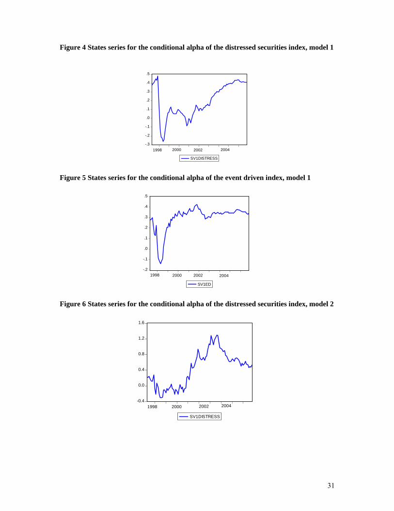
Obviously, many other patterns for the conditional alpha are possible, even in a pure

recursive model. Figures 4 and 5 give the profiles of the conditional alpha for respectively

the distressed securities and the event driven indices. The market collapse observed at the

beginning of the second millennium was a time of high return for these strategies, probably

because there were more business opportunities for them at this time in terms of business

failures, mergers, acquisitions or other special events.

Please insert figures 4 and 5 here


Model 2 is made up of equation (1), a model for the expectation of the excess return,

and of state equations (4) and (5) for the conditional alpha and beta. As revealed by table 3,

this model is an improvement over model 1. When shifting from model 1 to model 2, the

mean log likelihood statistic computed over the indices increases from -211.4 to -201.7 and

the mean AIC decreases from 4.03 to 3.90. This improvement is especially important for

the following indices: distressed securities, equity hedge and fund of funds.


Table 3 reveals that the conditional beta is much more manageable than the

conditional alpha. For the alpha, a Wald test reveals that the conditioning market variables

are significant as a group at the 5% level only for two strategies: the distressed securities

and the equity hedge13 ones. If we raise the significance level at 10%, we can add two more

strategies: the emerging markets and the macro strategies. For the other strategies, the

conditioning variables are not significant in their alpha equation, which might indicate that

a pure recursive model, even a random walk, is more appropriate for the alpha of those

strategies.

13 Let us recall that the equity hedge strategy is the most important category of hedge funds, with a market share of 30% in 2003.

19

Figure 6 shows the profile of the conditional alpha for the distressed securities index

in the context of model 2. Its pattern differs from its recursive profile (figure 4). In figure 4,

it increases continuously from the beginning of 2001 but in figure 6, it increases till the

middle of 2003 before undertaking a period of decrease.


The conditional alpha of the equity hedge index (figure 7) has the opposite profile,

decreasing from the middle of year 2000 to the beginning of 2003 and increasing thereafter.

Therefore, the distressed securities strategy seems to have benefited from the collapse of

the stock market from 2000 to 2002 while the equity hedge strategy suffered from this

situation. That may be explained quite obviously by the different nature of their respective

businesses. We also notice at figure 7 that the conditional alpha related to the equity hedge

strategy decreased substantially below 0 during the depression period of the stock market.


It remains that the improved goodness of fit of model 2 over model 1 is above all due

to the contribution of the two conditioning market variables for explaining the conditional

beta of the analyzed hedge fund strategies. Except for the market timing strategy, these

variables have an important role to play for explaining the conditional beta.

Once again, the behaviour of the conditional beta of the short sellers differs greatly

from the behaviour of the other categories of hedge funds. For these latter funds, an

increase in the interest rate is associated to a decrease of the conditional beta while an

increase in the market risk premium gives way to an increase of the conditional beta. These

sensitivities are quite rational. We notice no beta puzzle like Ferson and Schadt (1996) who

observed a negative relationship between the conditional beta and the market risk premium

while analysing mutual funds. They judged this behaviour quite perverse. We observe no

such behaviour here. The profile of the conditional beta of the hedge fund weighted

20

composite index, which is representative of the mean fund excluding the short sellers,

appears at figure 8.


Figure 8 shows a decrease in the conditional beta related to the weighted composite

index from the middle of 2000 to the beginning of 2003. Hedge funds took therefore less

risk during this period of weak stock markets. Thereafter, the beta returned to a more

normal level but remained well below the 0.50 quote observed at the end of the nineties.

The conditional beta associated to the short sellers strategy appears at figure 9.

Contrary to the majority of other funds, the shorts sellers increased their beta during the

period of weak markets in our sample, that is from the middle of 2000 to the beginning of

2003, to decrease it thereafter. Moreover, according to table 3, the short sellers increase

their beta when the risk premium decreases and when the interest rate increases. There

seems to be an apparent market puzzle here. But, for the short sellers, increasing their beta

comes to taking less risk because their beta is always negative. They thus reduced their

short selling activities during the period of weak markets. Therefore, the reaction of short

sellers to market conditions is the same as the other hedge funds: taking less risk when

market conditions deteriorate. It remains, as said before, that this behaviour might seem

perplexing for funds which short sell the market.



Model three is made up of the measurement equation (1), which is the equation of the

expected excess return, and of the two state equations (7) and (8) for the conditional alpha

and beta. Model 3 contains an additional conditioning variable in regard of model 2: the

squared market risk premium. The estimation of model 3 may be found at table 4.


21

Adding a market volatility variable as conditioning variable does not greatly improve

the fit, the mean likelihood statistic increasing from -201.7 to -197.4 and the mean AIC

decreasing from 3.90 to 3.86 when shifting from model 2 to model 3. There is however a

great improvement in the fit of the market timing equation.

The volatility variable has a significant impact at the 5% level for three indices:

equity market neutral, fund of funds and market timing. If we consider the 10% level of

significance, we can add two indices to this list: equity hedge and macro. The sign of this

variable is positive in the conditional beta equations of the indices and this indicates that

this variable is related to market timing operations. This variable is especially significant

for the market timing funds: these funds thus seem to succeed quite well in regard of their

vocation. For this last strategy, shifting from model 2 to model 3 increases the log

likelihood statistic from -210.8 to -192.4 and decreases the AIC criterion from 4.07 to 3.76.

Only for this strategy do we have such an improvement of fit when using model 3 instead

of model 2.

Please insert figures 10 and 11 here

Figure 10 gives the evolution of the conditional beta of market timers in model 2 and

figure 11, in model 3. A comparison of the filtered state series for the beta in model 3 with

the one of model 2 reveals the importance of the squared market risk premium to explain

the behaviour of the beta of market timers. According to figure 11, market timers decreased

their beta before the stock market collapse of the beginning of the second millennium and

increased it again before the recovery of the market, and that indicates the anticipatory

behaviour of these funds which gave way to good market timing. In 2005, when the market

became more volatile, market timers decreased moderately their beta.

22

4. Conclusion

In this paper, we revisit conditional return models in the dynamic setting of the Kalman

filter. This procedure appears more rigorous than the standard least squares procedure used

to compute the conditional alpha and beta (Racicot and Théoret 2008a). Indeed, these

coefficients are revised each period in an optimization framework taking into account all

information accumulated till this period. The least squares method has a great part of

arbitrariness because we may obtain a great variety of profiles for the conditional

coefficients depending on the conditioning information used. The dynamic optimization

process which is inherent to the Kalman filter removes some of this arbitrariness.

We resort to three state models to study the profile of the conditional alphas and betas

of the HFR returns over the period 1997-2005. In the first one, the state variables, which

are the conditional coefficients, are purely recursive. The other two state models aim at

studying the reaction of hedge funds to financial market information.

Our study reveals that the conditional alpha is not very sensitive to market news, except

for very specific strategies like the distressed securities one. Model 1, which considers a

purely recursive model for the conditional alpha, seems more appropriate for this

coefficient than the other two which incorporate conditioning market information. The

profile of the conditional alpha thus seems in line with the efficient market hypothesis. At

the limit, the alpha follows a random walk.

But the situation is very different for the conditional beta which appears to be much

more manageable than the conditional alpha. For most of the hedge fund indices analysed

in this study, the conditional beta responds positively to the market risk premium and

negatively to the level of interest rate, a rational behaviour. Moreover, the betas are

conditioned by a cycle which may be explained quite easily by the profile of

macroeconomic variables. Incidentally, the performance of models integrating conditioning

23

information is usually much better to explain the expected excess returns of the hedge

funds because the conditional beta is significantly related to market news or

macroeconomic information. Finally, we propose a possible framework to account for the

biases that might be caused by errors-in-variables in the setting of the Kalman Filter. This

approach might be justified by the fact that financial variables might be contaminated by

measurement errors thus causing a bias in the estimation process. Several authors have

worked on the subject (Racicot & Théoret, 2008a, b and others) and there is strong

evidence of that problem. We thus think that it is a good idea to do further research on how

to implement efficiently in the Kalman Filter another algorithm to account for measurement

errors.

24

References

Bassett, G.W., V.G. France and S.R. Pliska (1991), "Kalman Filter Estimation for Valuing Nontrading Securities, with Applications to MMI Cash Future Spread on October 19 and 20, 1987", Review of Quantitative Finance and Accounting, 1 (2), 135-151.

Berkelaar, A., Kobor, A., and Kouwenberg, R. (2009), "Asset allocation for hedge fund strategies: How to better manage tail risk". In: Gregoriou, G.N. (ed.), The VaR Modeling Handbook, New York : McGraw-Hill.

Bollen, N.P.B. and R. Whaley (2006), "Hedge Fund Risk Dynamics: Implications for Performance Appraisal", Working Paper, Vanderbilt University.

Capocci, D. and G. Hübner (2004), "Analysis of hedge fund performance", Journal of Empirical Finance, 11, 55-89.

Carhart, M.M. (1997), "On persistence in mutual fund performance", Journal of Finance, 52, 57-82.

Christopherson, J.A., W.E. Ferson, and D.A. Glassman (1998), "Conditioning manager alphas on economic information: another look at the persistence of performance", Review of Financial Studies, 11, 111-142.

Cochrane, J.H. (2005), Asset Pricing, Revised edition, Princeton University Press. Coën, A., Racicot, F.E. (2007), "Capital Asset Pricing Models Revisited: Evidence

from Errors in Variables", Economics Letters, Vol. 95 (3), 443-450. Coën, A., Racicot, F.E. and R. Théoret (2006a), "Hedge Funds Returns, Higher

Moments and Nonlinear Risk", in: Gregoriou, G.N. and D. Kaiser (eds.), Hedge Funds and Managed Futures: a Handbook for Institutional Investors, Risk Books.

Coën, A., Racicot, F.E. and R. Théoret (2006b), "Higher Moments as Risk Instruments to Discard Errors in Variables: the Case of the Fama and French Model", Proceedings of the Global Finance Association.

Fama, E.F. and K.R. French (1992), "The cross-section of expected stock returns", Journal of Finance, 47, 427-465.

Fama, E.F. and K.R. French (1993), "Common risk factors in the returns on stocks and bonds", Journal of Financial Economics, 33, 3-56.

Fama, E.F. and K.R. French (1997), "Industry costs of equity", Journal of Financial Economics, 43, 153-193.

Fama, E.F. and M.R. Gibbons (1982), "Inflation, Real Returns and Capital Investment", Journal of Monetary Economics, 9, 297-323.

Ferson, W.E. and M. Qian, (2004), "Conditional Evaluation Performance: Revisited", The Research Foundation of CFA Institute.

Ferson, W.E., and R.W. Schadt (1996), "Measuring fund strategy and performance in changing economic conditions", Journal of Finance, 51, 425-461.

Gregoriou, G.N. (2009), “Book Review of: The Econometric Analysis of Hedge Fund returns: An Errors-in-Variables Perspective by: F.E. Racicot and R. Théoret, Journal of Wealth Management, 12 (2), 138-140.

Hsieh, D.A. and N. Kulatilaka (1982), "Rational Expectations and Risk Premia in Forward Markets: Primary Metals at the London Metals Exchange", Journal of Finance, 37, 1199-1207.

L'Habitant, F. (2004), Hedge Funds: Quantitative Insights, Wiley. Ljungqvist, L., Sargent, T.J. (2004), Recursive Macroeconomic Theory. Second

Edition, Massachusetts: MIT Press.

25

Mamaysky, H., Spiegel, M., and Zhang, H. (2008). "Estimating the dynamics of mutual fund alpha and betas". Review of Financial Studies, 21 (1), 233-264.

Mamaysky, H., Spiegel, M., and Zhang, H. (2007). "Improved forecasting of mutual

fund alpha and betas". Review of Finance, 11(3), 1-42.

Pennacchi, G.G., (1991) "Identifying the dynamics of real interest rates and inflation: Evidence using survey data", Review of Financial Studies, 4(1), 53- 86.

Rachev, S.T., S. Mittnik, F.J. Fabozzi, S.M. Focardi and T. Jasic (2007), Financial Econometrics, Wiley.

Racicot, F.E. and R. Théoret (2009), "Integrating Volatility Factors in The Analysis of The Hedge Fund Alpha Puzzle", Journal of Asset Management, 10 (1), 37-62.

Racicot, F.E. and R. Théoret (2008a), "Conditional financial models and the alpha puzzle: A panel study of hedge fund retunrs", Journal of Wealth Management, 11 (2), 59-77.

Racicot, F.E. and R. Théoret (2008b), The Econometric Analysis of Hedge Fund returns: An Errors-in-Variables Perspective, Netbiblo.

Racicot, F.E. and R. Théoret (2007), “A study of dynamic market strategies of hedge funds using the Kalman filter”, Journal of Wealth Management, 10 (3), 94-106.

Racicot, F.E. and R. Théoret (2006a), Finance computationnelle et gestion des risques, Presses de l'Université du Québec (PUQ).

Racicot, F.E. and R. Théoret (2006b), "On Comparing Hedge Fund Strategies Using Higher Moment Estimators for Correcting Specification Errors in Financial Models", in : Gregoriou, G.N. and D. Kaiser (eds.), Hedge Funds and Managed Futures: a Handbook for Institutional Investors, Risk Books.

Swinkels, L.A.P. and P.J. van der Sluis (2001), "Return-based style analysis with time-varying exposure", Working Paper, Tilburg University.

Treynor J. and K. Mazuy (1966), "Can Mutual Funds Outguess the Market", Harvard Business Review, 44.

Whaley, R.E.(2006), Derivatives: Markets, Valuation and Risk Management, Wiley.

26

Tables

Table 1 Descriptive statistics of the HFR indices returns, 1997-2005*

* The statistics appearing in this table are computed on the monthly returns of the HFR indices over the period running from January 1997 to December 2005. The weighted composite index is computed over the whole set of the HFR indices. The CAPM beta is estimated using the simple market model, that is: ( ) itftmtftit RRRR εβα +−+=− , where Ri is the return of the index i, Rm is the S&P500 return, Rf is the

riskless rate and εi is the innovation.

Mean Median s.-d. MAX MIN Skew Kurtosis CAPM-

beta

Distressed securities 0.95 1.00 1.82 5.34 -8.88 -1.38 10.26 0.21 Emerging 1.19 1.77 4.82 15.75 -22.07 -0.97 7.57 0.71 Equity hedge 1.10 1.18 3.07 11.54 -7.42 0.35 4.24 0.52 Equity Market Neutral 0.66 0.52 1.16 3.88 -3.90 0.04 5.33 0.03 Equity non hedge 1.10 1.44 4.65 12.50 -15.52 -0.27 3.95 0.85 Event driven 1.00 1.14 2.18 5.93 -9.81 -1.21 7.89 0.36 Fund of funds 0.72 0.68 1.48 5.46 -6.09 -0.24 7.41 0.20 Macro 0.76 0.80 2.04 6.24 -4.27 0.22 3.36 0.16 Market timing 1.02 0.91 2.34 6.91 -3.20 0.18 2.28 0.37

Short seller 0.33 0.23 7.13 26.43 -21.00 0.43 5.80 -1.22

Mean of indices 0.88 0.96 3.07 10.00 -10.22 -0.28 5.81 0.22

Weighted composite 0.95 0.96 2.32 7.62 -8.31 -0.27 4.91 0.41

S&P500 0.72 0.93 4.64 9.78 -14.44 -0.48 3.23 1.00

27

Table 2: Kalman filter estimation of model 1*

sv1 sv2 smb hml L AIC

Distressed securities 0.4096 0.2329 0.2050 0.1341 -202.48 3.84 3.17 8.67 5.70 3.59 Emerging 0.3125 0.7079 0.3810 0.1761 -292.66 5.53 1.04 11.35 5.62 2.00 Equity hedge 0.5207 0.4603 0.2669 -0.0228 -194.17 3.69 4.36 18.53 9.43 -0.58 Equity Market neutral 0.2837 0.0492 0.0730 0.0762 -179.28 3.41 2.73 2.28 2.94 2.49 Equity non hedge 0.3189 0.7608 0.4198 -0.0127 -193.65 3.72 2.73 31.37 14.87 -0.32 Event driven 0.3422 0.3940 0.2366 0.1789 -166.36 3.17 3.68 20.39 9.46 5.53 Fund of funds 0.2471 0.1993 0.1591 0.0622 -161.27 3.15 2.79 10.83 6.75 2.19 Macro 0.2219 0.1816 0.1875 0.1478 -231.50 4.46 1.31 5.16 4.84 2.89 Market timing 0.5685 0.3347 0.0745 -0.0343 -213.39 4.04 3.97 11.26 2.14 -0.64 Short seller 0.4030 -0.9293 -0.4442 0.4398 -279.25 5.28

1.52 -16.89 -7.95 6.20

Weighted composite 0.4061 0.3737 0.2067 0.0192 -159.20 3.03

4.68 20.71 9.16 0.64 * Model 1 is made up of the measurement equation (1) and transition equations (2) and (3). These

equations are estimated simultaneously resorting to the Kalman filter. For each strategy, the first line of numbers is the estimated coefficients of the variables located at the head of the columns and the second line gives the corresponding t-statistics (in italics). The L statistic is the log likelihood associated to an estimation. The sv1 coefficient is the final state of the conditional alpha and the sv2 coefficient is the final state of the conditional beta.

28


conditional alpha conditional beta

sv1 rf(-1) mkt_rf(-1) sv2 rf(-1) mkt_rf(-1) smb hml L AIC

Distressed securities 0.4748 0.0388 -0.0216 0.2148 -0.0090 0.0047 0.2007 0.1709 -189.66 3.68 4.14 2.54 -2.84 9.02 -3.19 3.93 6.43 4.71 Emerging 1.3888 0.1061 -0.0101 0.6067 -0.0253 0.0097 0.3712 0.2553 -279.93 5.36 5.21 2.14 -0.47 10.96 -2.76 2.75 5.00 2.46 Equity hedge 0.3047 -0.0481 0.0176 0.5548 -0.0044 0.0061 0.2885 0.0458 -173.85 3.38 3.08 -2.83 1.95 27.00 -1.36 3.56 10.93 1.11 Equity Market neutral 0.3623 -0.0111 0.0130 -0.0329 -0.0080 0.0006 0.0888 0.1002 -171.88 3.34 3.73 -0.72 1.70 -1.63 -3.05 0.47 3.53 3.25 Equity non hedge 0.5149 -0.0028 0.0133 0.7020 -0.0104 0.0029 0.4348 0.0297 -182.22 3.54 4.82 -0.15 1.63 31.60 -2.69 1.66 12.96 0.56 Event driven 0.3859 0.0041 0.0010 0.3210 -0.0068 0.0006 0.2448 0.1954 -162.12 3.16 4.32 0.33 0.15 17.30 -2.72 0.50 9.17 5.38 Fund of funds 0.3293 -0.0042 0.0077 0.1591 -0.0087 0.0029 0.1718 0.1011 -148.37 2.90 4.20 -0.35 1.21 9.78 -3.55 2.25 7.29 2.81 Macro 0.0393 0.0215 -0.0226 0.1169 -0.0082 0.0023 0.1903 0.1728 -227.14 4.38 0.24 1.06 -2.25 3.46 -1.83 1.21 4.55 3.08 Market timing 0.7051 -0.0187 0.0196 0.3304 0.0000 -0.0006 0.0820 -0.0322 -210.83 4.07 5.05 -0.80 1.81 11.38 -0.01 -0.41 2.24 -0.59 Short seller 0.3018 -0.0157 0.0039 -0.8569 0.0211 -0.0087 -0.4645 0.3429 -271.10 5.20

1.23 -0.35 0.19 -16.81 2.83 -2.61 -7.93 3.92

Weighted composite 0.3986 -0.0139 0.0089 0.3482 -0.0074 0.0028 0.2215 0.0586 -146.60 2.87

5.17 -1.08 1.32 21.75 -2.68 1.85 9.04 1.49 * Model 2 is made up of the measurement equation (1) and transition equations (4) and (5). These equations are estimated simultaneously

resorting to the Kalman filter. For each strategy, the first line of numbers is the estimated coefficients of the variables located at the head of the columns and the second line gives the corresponding t-statistics (in italics). The L statistic is the log likelihood associated to an estimation. The sv1 coefficient is the final state of the conditional alpha and the sv2 coefficient is the final state of the conditional beta.

29


conditional alpha conditional beta

sv1 rf(-1) mkt_rf(-1) mkt_rf(-1)2 sv2 rf(-1) mkt_rf(-1) mkt_rf(-1)2 smb hml L AIC

Distressed securities 0.5631 -0.1841 -0.0137 0.0024 0.1904 -0.0162 0.0045 0.0001 0.2093 0.1705 -185.28 3.63 5.13 -2.29 -1.69 2.70 8.35 -0.97 2.54 0.37 7.10 4.69 Emerging 1.3945 0.0048 -0.0079 0.0011 0.6069 -0.0326 0.0097 0.0001 0.3731 0.2545 -279.81 5.40 5.23 0.02 -0.32 0.46 10.95 -0.70 2.28 0.15 5.02 2.39 Equity hedge 0.2466 -0.0871 0.0190 0.0004 0.6311 -0.0414 0.0077 0.0004 0.2820 0.0306 -170.77 3.36 2.54 -0.91 1.83 0.38 31.31 -1.80 3.48 1.62 9.93 0.70 Equity Market neutral 0.2623 0.0164 0.0118 -0.0003 0.0649 -0.0491 0.0025 0.0005 0.0785 0.0826 -168.20 3.31 2.77 0.19 1.46 -0.31 3.30 -2.57 1.75 2.11 3.13 2.63 Equity non hedge 0.4608 0.0316 0.0120 -0.0004 0.7489 -0.0284 0.0038 0.0002 0.4293 0.0217 -181.56 3.56 4.34 0.31 1.24 -0.33 33.92 -1.02 1.73 0.66 12.03 0.38 Event driven 0.4106 -0.1189 0.0053 0.0013 0.3322 -0.0217 0.0010 0.0002 0.2472 0.1907 -159.37 3.15 4.72 -1.60 0.76 1.69 18.38 -1.54 0.66 1.04 8.92 5.20 Fund of funds 0.3307 -0.0909 0.0112 0.0010 0.1998 -0.0341 0.0038 0.0003 0.1726 0.0971 -144.73 2.87 4.36 -1.41 1.70 1.41 12.68 -2.48 2.76 1.91 7.27 2.61 Macro -0.0441 -0.0584 -0.0200 0.0009 0.2296 -0.0645 0.0047 0.0007 0.1814 0.1500 -224.37 4.36 -0.28 -0.44 -1.62 0.58 6.97 -1.96 1.72 1.76 3.87 2.37 Market timing 0.4339 -0.0059 0.0187 -0.0002 0.6145 -0.1248 0.0051 0.0015 0.0537 -0.0847 -192.04 3.76 3.70 -0.07 2.22 -0.20 25.24 -6.07 2.64 5.87 1.81 -1.90 Short seller 0.3382 -0.1856 0.0099 0.0019 -0.8434 0.0015 -0.0082 0.0002 -0.4612 0.3367 -270.44 5.22

1.39 -0.86 0.47 0.73 -16.65 0.04 -2.08 0.43 -7.84 3.81

Weighted composite 0.4082 -0.0945 0.0118 0.0009 0.3647 -0.0213 0.0033 0.0002 0.2219 0.0537 -144.65 2.87

5.38 -1.23 1.57 1.08 23.15 -1.19 2.10 0.80 8.65 1.33 * Model 3 is made up of the measurement equation (1) and transition equations (7) and (8). These equations are estimated simultaneously resorting to the Kalman filter. For each strategy, the first line of numbers is the estimated coefficients of the variables located at the head of the columns and the second line gives the corresponding t-statistics (in italics). The L statistic is the log likelihood associated to an estimation. The sv1 coefficient is the final state of the conditional alpha and the sv2 coefficient is the final state of the conditional beta.

30

Figures

Figure 1 State series for the conditional beta of the HFR weighted composite index, model 1

.36

.38

.40

.42

.44

.46

.48

SV2FWC

1998 2000 2002 2004

Figure 2 State series for the conditional beta of the short sellers index, model 1

-1.3

-1.2

-1.1

-1.0

-0.9

-0.8

-0.7

SV2SS

1998 2000 2002 2004

Figure 3 States series for the conditional alpha of the hedge fund weighted composite index, model 1

.0

.1

.2

.3

.4

.5

.6

.7

SV1FWC

1998 2000 2002 2004

31

Figure 4 States series for the conditional alpha of the distressed securities index, model 1

-.3

-.2

-.1

.0

.1

.2

.3

.4

.5

SV1DISTRESS

1998 2000 2002 2004

Figure 5 States series for the conditional alpha of the event driven index, model 1

-.2

-.1

.0

.1

.2

.3

.4

.5

SV1ED

1998 2000 2002 2004

Figure 6 States series for the conditional alpha of the distressed securities index, model 2

-0.4

0.0

0.4

0.8

1.2

1.6

SV1DISTRESS

1998 2000 2002 2004

32

Figure 7 States series for the conditional alpha of the equity hedge index, model 2

-0.5

0.0

0.5

1.0

1.5

SV1EQHEDGE

1998 2000 2002 2004

Figure 8 State series for the conditional beta of the HFR weighted composite index, model 2

.20

.25

.30

.35

.40

.45

.50

.55

SV2FWC

1998 2000 2002 2004

Figure 9 State series for the conditional beta of the short sellers index, model 2

-1.4

-1.3

-1.2

-1.1

-1.0

-0.9

-0.8

-0.7

-0.6

-0.5

SV2SS

1998 2000 2002 2004

33

Figure 10 State series for the conditional beta of the market timers, model 2

.2

.3

.4

.5

.6

SV2MT

1998 2000 2002 2004

Figure 11 State series for the conditional beta of the market timers, model 3

.0

.1

.2

.3

.4

.5

.6

.7

.8

.9

SV2MT

1998 2000 2002 2004

cahier de recherche 2009-06 - uqam(2007), chap.11. as said by l'habitant (2004), the kalman is...

Documents