calculate absorption profiles? experimental spectrum calculated spectrum for candidate molecule
TRANSCRIPT
Vibronic coupling and the computational modelling of electronic spectra
1. The Born-Oppenheimer approximation and the adiabatic potential energy surface
2. The Franck-Condon approximation
3. Breakdown of the simple Born-Oppenheimer picture - ``Vibronic coupling’’
4. Diabatic potential energy surfaces and a simplified model of spectroscopy
5. Complicated adiabatic surfaces and couplings
6. The model Hamiltonian approach of Köppel, Domcke and Cederbaum (KDC)
7. Application to NO2 molecule (photoelectron and electronic spectra)
Lecture I, Frontiers in Spectroscopy, Columbus, 1/2007

The molecular Hamiltonian
H = Te + Tn + Vne + Vee + Vnn
Electrons and nuclei treated on an equal footing
Qualitatively inconsistent with our models and thinking about molecules in chemistry
Does not lend itself to eigenstates described as “electronic”, “vibrational” and “rotational””
Where is the notion of molecular structure?
Example: Ozone
H = ∑ Te + ∑ Tn + ∑∑ Vne + 1/2 ∑∑ Vee + 1/2 ∑∑ Vnn
i i
i j Where is the “unique” oxygen?What is the bond length?
O O O
+
-

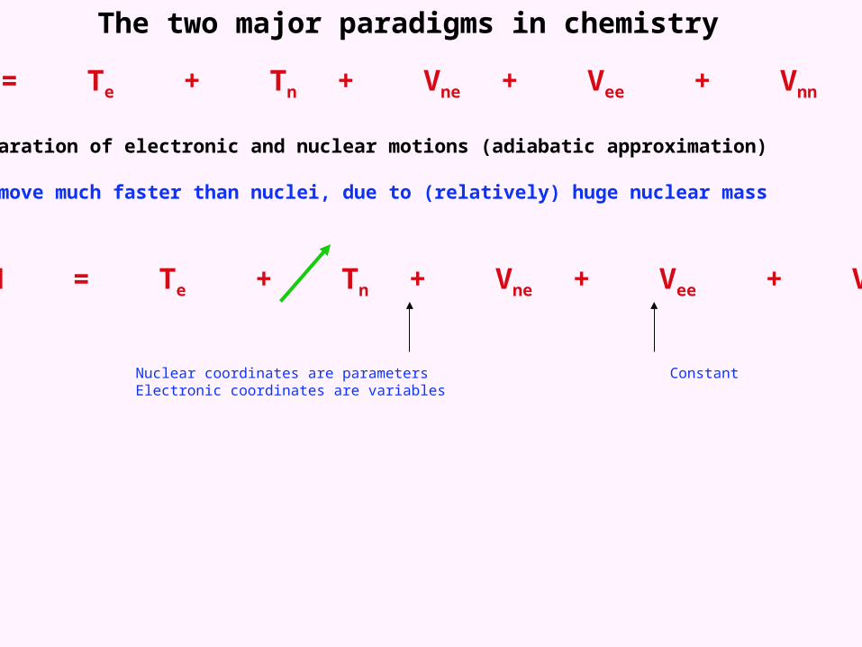
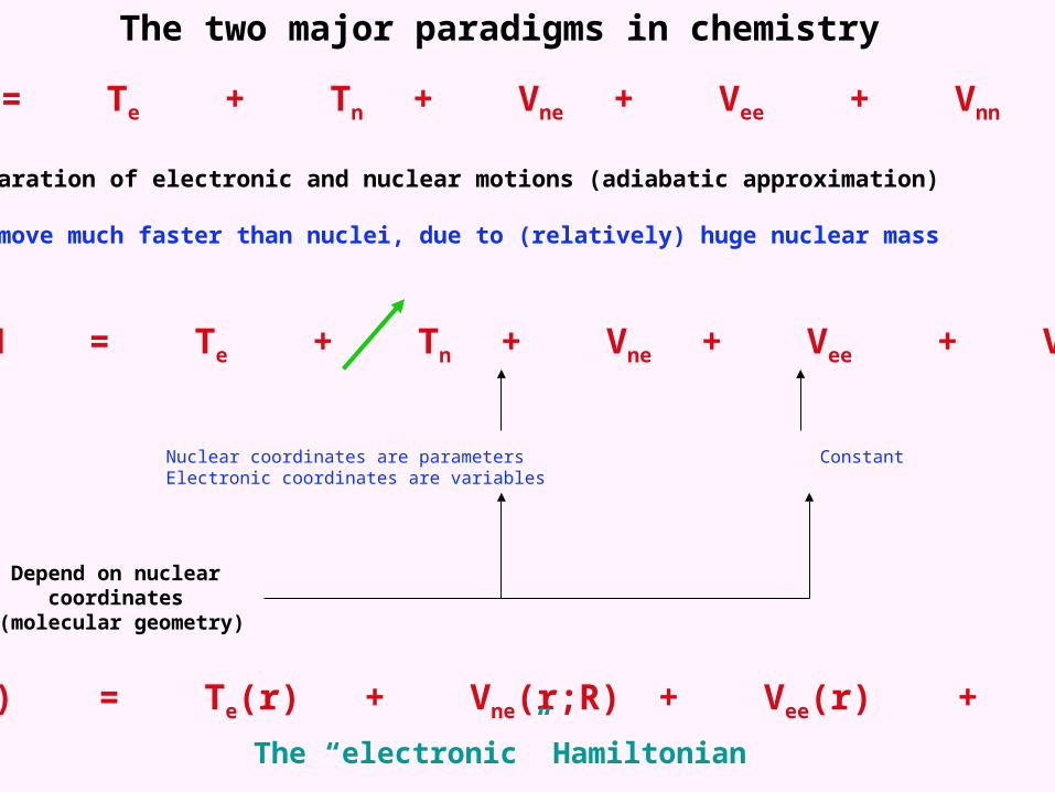
The two major paradigms in chemistry
H = Te + Tn + Vne + Vee + Vnn

The two major paradigms in chemistry
H = Te + Tn + Vne + Vee + Vnn
1. The separation of electronic and nuclear motions (adiabatic approximation)
Electrons move much faster than nuclei, due to (relatively) huge nuclear mass
H = Te + Tn + Vne + Vee + Vnn

The two major paradigms in chemistry
H = Te + Tn + Vne + Vee + Vnn
1. The separation of electronic and nuclear motions (adiabatic approximation)
Electrons move much faster than nuclei, due to (relatively) huge nuclear mass
H = Te + Tn + Vne + Vee + Vnn
Nuclear coordinates are parametersElectronic coordinates are variables
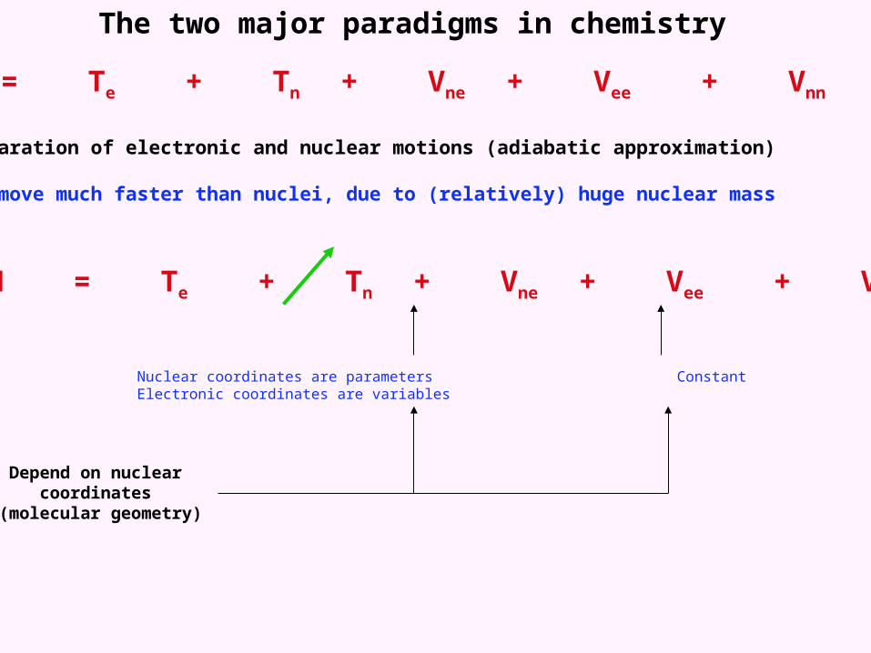
The two major paradigms in chemistry
H = Te + Tn + Vne + Vee + Vnn
1. The separation of electronic and nuclear motions (adiabatic approximation)
Electrons move much faster than nuclei, due to (relatively) huge nuclear mass
H = Te + Tn + Vne + Vee + Vnn
Nuclear coordinates are parameters Constant Electronic coordinates are variables
Depend on nuclear coordinates (molecular geometry)
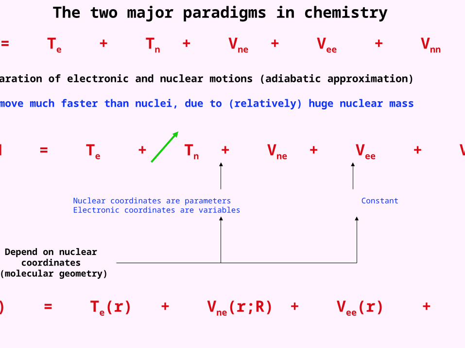
Helec(r) = Te(r) + Vne(r;R) + Vee(r) + Vnn
The “electronic” Hamiltonian

Helec(r) = Te(r) + Vne(r;R) + Vee(r) + Vnn
Helec(r) = ∑ [ Te(r) + Vne(r;R) ] + ∑∑ Vee(r) + Vnn
= ∑ Hi + ∑∑ Hij + Vnn

Helec(r) = Te(r) + Vne(r;R) + Vee(r) + Vnn
Helec(r) = ∑ [ Te(r) + Vne(r;R) ] + ∑∑ Vee(r) + Vnn
= ∑ Hi + ∑∑ Hij + Vnn
The “one electron” Electron-electron Hamiltonian repulsion

A reminder from quantum mechanics:
if…
H = ∑ hi
then…
= i
Each term must involve independent coordinates
“Separability condition”

Helec(r) = Te(r) + Vne(r;R) + Vee(r) + Vnn
Helec(r) = ∑ [ Te(r) + Vne(r;R) ] + ∑∑ Vee(r) + Vnn
= ∑ Hi + ∑∑ Hij + Vnn
2. The neglect of “electron correlation” - the independent particle approximation
= ∑ Hi + ∑vieff
+ Vnn
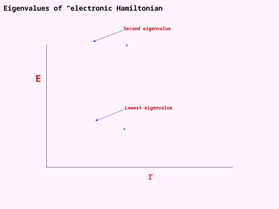
Eigenvalues of “electronic Hamiltonian”
E
r
x
x
Lowest eigenvalue
Second eigenvalue

Eigenvalues of “electronic Hamiltonian”
E
r
x x x x x x
x
x x x x x x x x x x x x x

Adiabatic potential energy surfaces
E
r
x x x x x x
x
x x x x x x x x x x x x x

Adiabatic potential energy surfaces
E
r
x x x x x x
x
x x x x x x x x x x x x x
Equilibrium bond length (re)
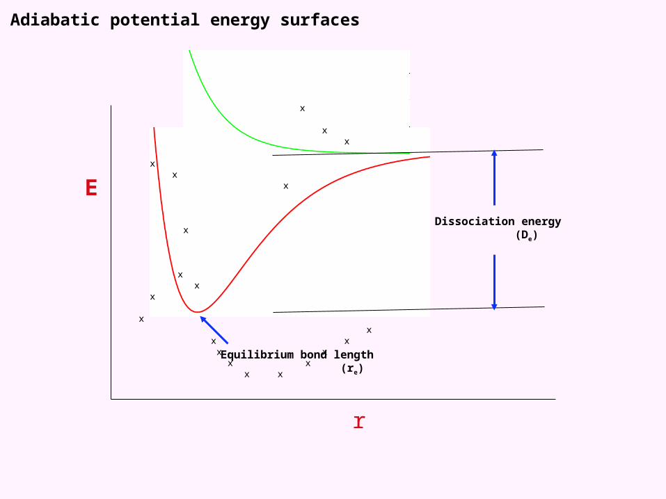
Adiabatic potential energy surfaces
E
r
x x x x x x
x
x x x x x x x x x x x x x
Equilibrium bond length (re)
Dissociation energy (De)

Adiabatic potential energy surfaces
E
r
x x x x x x
x
x x x x x x x x x x x x x
Equilibrium bond length (re)
Dissociation energy (De)
Vertical excitation energy

H(r,R) = Helec(r;R) + Hnuc(R)
Hnuc(R) = Tnuc(R) + V(R)
= elec nuc
elec vibrot
E = Eelec + Evib + Erot
The Born-Oppenheimer Separation:
Adiabatic potential energy surface (PES)
Note: elec diagonalizes electronic Hamiltonian nuc diagonalizes nuclear Hamiltonian
B.O. approximation assumes that diagonalizes full Hamiltonian

Adiabatic potential energy surfaces
E
r
x x x x x x
x
x x x x x x x x x x x x x
Equilibrium bond length (re)
Dissociation energy (De)
Vertical excitation energy
2B0Zero-pointEnergy (ZPE)

H = Te + Tn + Vne + Vee + Vnn
Qualitatively inconsistent with our models and paradigms in chemistDoes not lend itself to eigenstates described as “electronic”, “vibrational” and “rotational”Where is the structure?
Born-Oppenheimerapproximation
Independent electron approximation

The “crude” Born-Oppenheimer approximation and electronic spectroscopy
-Ignore R dependence of electronic wavefuction
ve = e(r;R0) v(R)
-Spectroscopic transition moments in dipole approximation
M = <ve’’ | | ve
‘>
M = < e’’(r;R0) v
’’(R) | n + e | e’(r;R0) v
’(R)>
= < e’’(r;R0) | e | e
’(r;R0) > < v’’(R) | v
’(R) > >
+ < v’’(R) | n | v
’(R) > < e”(r;R0) | e
’(r;R0) >
Reference geometry
=0

The “crude” Born-Oppenheimer approximation and electronic spectroscopy
-Ignore R dependence of electronic wavefuction
ve = e(r;R0) v(R)
-Spectroscopic transition moments in dipole approximation
M = <ve’’ | | ve
‘>
M = < e’’(r;R0) v
’’(R) | n + e | e’(r;R0) v
’(R)>
= < e’’(r;R0) | e | e
’(r;R0) > < v’’(R) | v
’(R) > >
Reference geometry
Electronic transition moment
Vibrational overlap integral
The Franck-Condon approximation
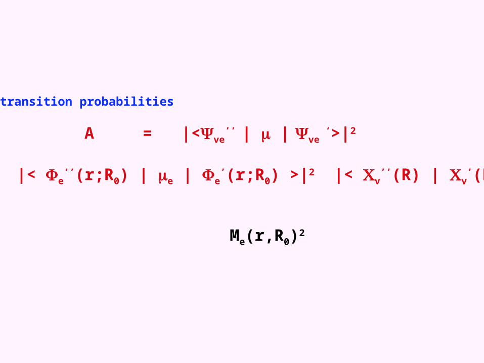
-Spectroscopic transition probabilities
A = |<ve’’ | | ve
‘>|2
A = |< e’’(r;R0) | e | e
’(r;R0) >|2 |< v’’(R) | v
’(R) >|2
Me(r,R0)2 FCF
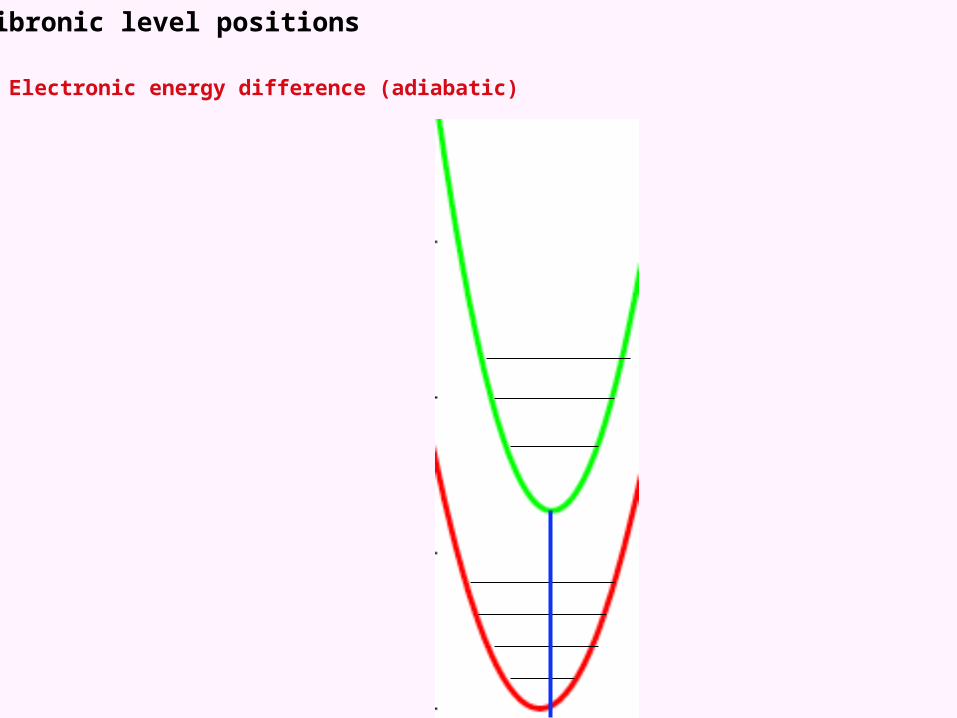
Vibronic level positions
Electronic energy difference (adiabatic)

Vibronic level positions
Electronic energy difference - ZPE of ground state
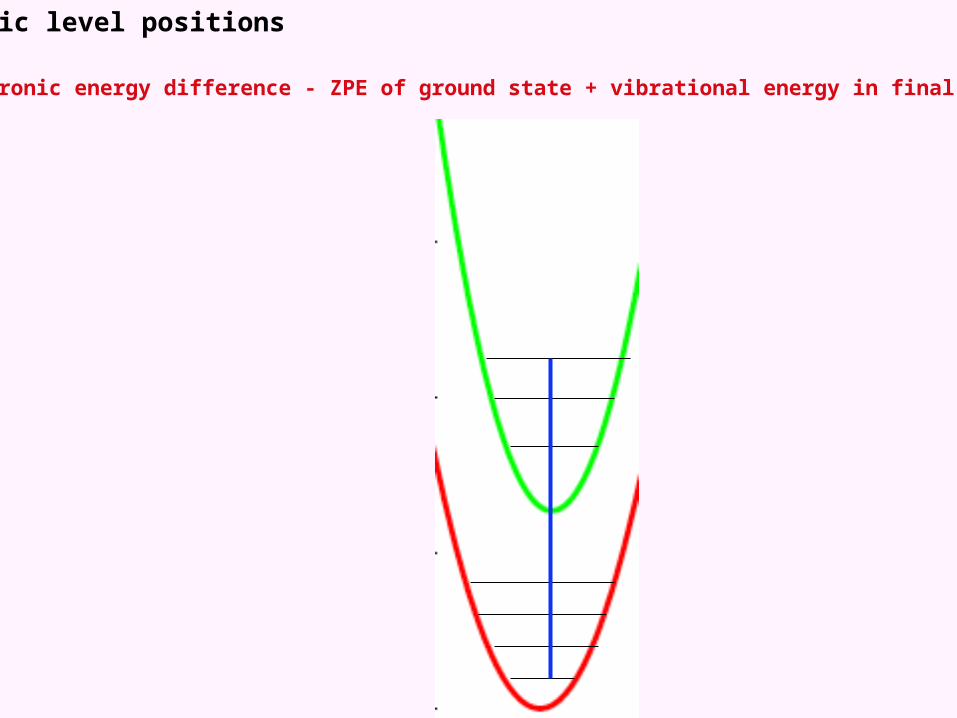
Vibronic level positions
Electronic energy difference - ZPE of ground state + vibrational energy in final state

Vibronic level positions
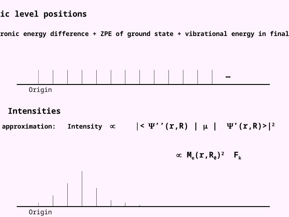
Electronic energy difference + ZPE of ground state + vibrational energy in final state
Origin

Vibronic level positions
Electronic energy difference + ZPE of ground state + vibrational energy in final state
Origin
Intensities
Dipole approximation: Intensity |< ’’(r,R) | | ’(r,R)>|2
Me(r,R0)2 Fk
Vibronic level positions
Electronic energy difference + ZPE of ground state + vibrational energy in final state
Origin
Intensities
Dipole approximation: Intensity |< ’’(r,R) | | ’(r,R)>|2
Me(r,R0)2 Fk
Origin
…

Origin
Origin
…
0 1 2 3 4 5 6
1 2 3
With several modes …

To do a Franck-Condon simulation, we need:
Quantum chemical calculation of ground state geometry and force field
“EASY” - CAN BE DONE WITH ANY METHOD
Quantum chemical calculation of excited state geometry and force field
MORE CARE REQUIRED WITH RESPECT TO CHOICE OF METHOD (CIS, RPA, CIS(D), MCSCF, CASPT2, EOM-CC, MRCI)
(balance is important here)
Quantum chemical calculation of transition dipole moment
NOT SO HARD - ACCURACY USUALLY NOT VERY IMPORTANT
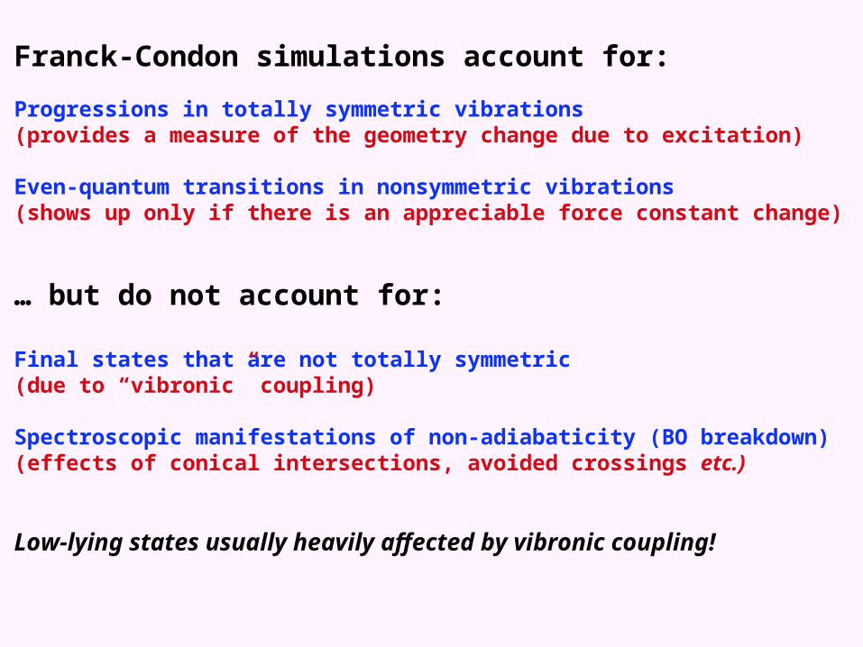
Franck-Condon simulations account for:
Progressions in totally symmetric vibrations (provides a measure of the geometry change due to excitation)
Even-quantum transitions in nonsymmetric vibrations(shows up only if there is an appreciable force constant change)
… but do not account for:
Final states that are not totally symmetric(due to “vibronic” coupling)
Spectroscopic manifestations of non-adiabaticity (BO breakdown)(effects of conical intersections, avoided crossings etc.)
Low-lying states usually heavily affected by vibronic coupling!
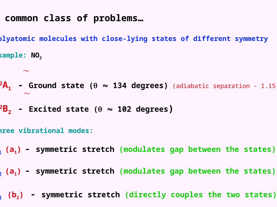
A common class of problems…
Polyatomic molecules with close-lying states of different symmetry
Example: NO2
X2A1 - Ground state ( 134 degrees)
A2B2 - Excited state ( 102 degrees)
Three vibrational modes:
1 (a1) - symmetric stretch (modulates gap between the states))
2 (a1) - symmetric stretch (modulates gap between the states)
3 (b2) - symmetric stretch (directly couples the two states)
(adiabatic separation - 1.15 eV)

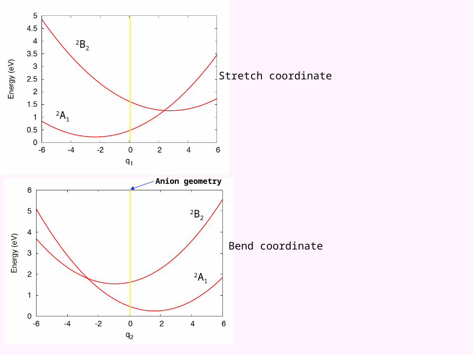
The adiabatic potential energy surface(s) of NO2
One dimensional representations
O
N
O
2A1
2B2
2A1
2B2
Stretch coordinate
Bend coordinate
Anion geometry


The adiabatic potential energy surface(s) of NO2
Two dimensional representations
O
N
O

q1
q2
2A1 minimum
2B2 minimum

q1
q2
2A1 minimum
2B2 minimum

q1
q2
Conical intersection seam
Seam minimum

q1
q2
Conical intersection seam
Seam minimum

Upper adiabatic sheet (cone state)
Lower adiabatic sheet
2A1 state
2B2 state
States of different symmetry can interconvert on same adiabatic surface! (pseudorotation)
Rapidlychangingingwavefunction

Top view
2B2 minimum
Vertex ofcone state

Obviously, adiabatic potential energy surfaces in these cases areexceedingly complicated -- mathematically they are nondifferentiablealong the conical intersection seam, and very far from the parabolic ideal…
Moreover … the adiabatic states that diagonalize the electronic Hamiltonianvary rapidly near the conical intersection; the off-diagonal matrix elements ofthe nuclear kinetic energy operator are no longer negligible. Equivalently, they are poor approximations to eigenfunctions of the nuclear kinetic energy operator -- wavefunction is varying rapidly in the region of an intersection(recall diatomic curves)
This means that the Born-Oppenheimer approximation is not very good here, and our simple idea of the separable wavefunction, the Franck-Condonapproximation, and all that goes with this, will no longer give us a good model for understanding spectra
ve ≠ e(r;R0) v(R)

Going beyond the crude Born-Oppenheimer approximation:
The “adiabatic approximation”
ve;i = c;i e(r;R0) c;i (R)
The ``crude Born-Huang” expansion:
ve;i = c;i e(r;R0) (R)
(A formally exact expansion for the vibronic wavefunction)
The adiabatic approximation - which is the “Born-Oppenheimer” approximationto most quantum chemists allows for variation of the electronic wavefunction withR, but is difficult to apply to spectroscopy and separability of vibrational and electronic parts
The crude Born-Huang expansion provides a convenient formalism for vibroniccoupling, and we will use it in the following.
Wavefunctions calculated from quantum chemistry(R dependence carried by coefficients)

“Diabaticity and quasi-diabaticity”
The electronic states appearing in the crude Born-Huang expansion are strictly andrigorously diabatic (they diagonalize the nuclear kinetic energy operator - for obvious reasons) and the treatment of vibronic coupling we are about to study is exact in principle.
However… implementation of a theory based strictly on the CBH expansion is clearly a daunting and terrible prospect -- so many electronic states have to be considered (think even about dissociation of a diatomic)
The (usually quite) slow variation of electronic wavefunctions with R can be viewed as aconsequence of a mixing-in of many functions in the frozen basis as the nuclei move, andIs NOT due exclusively (or even substantially) to mixing with those states that are strongly coupled vibronically. Hence, we can make an approximation in the formalismthat accounts for this.
“Diabaticity and quadi-diabaticity”
The electronic states appearing in the crude Born-Huang expansion are strictly andrigorously diabatic (they diagonalize the nuclear kinetic energy operator - for obvious reasons) and the treatment of vibronic coupling we are about to study is exact in principle.
However… implementation of a theory based strictly on the CBH expansion is clearly a daunting and terrible prospect -- so many electronic states have to be considered (think even about dissociation of a diatomic)
The (usually quite) slow variation of electronic wavefunctions with R can be viewed as aconsequence of a mixing-in of many functions in the frozen basis as the nuclei move, andIs NOT due exclusively (or even substantially) to mixing with those states that are strongly coupled vibronically. Hence, we can make an approximation in the formalismthat accounts for this.

The vibronic Hamiltonian in pictures…
Diabaticelectronic basis
Adiabaticelectronic basis
H(R) = +
H(R) = +
TN V
Diabatic wavefunctions do not change with nuclear displacement, necessitatingenormous configuration expansions.
Consider the case where a few states are strongly coupled vibronically, and relativelyisolated from the rest.

The vibronic Hamiltonian in pictures…
Quasidiabaticelectronic basis
H(R) = +
H(R) = +
TN VMixing of the orthogonal complement with the coupled diabatic states (via the blockdiagonalization) allows for the smooth variation of the wavefunction associated with“nuclei following”. The resultant weak nuclear coupling with other states is small andit is reasonable to neglect it. Which leads to the KDC model Hamiltonian…
Block diagonalize potential energy
Diabaticelectronic basis

The vibronic Hamiltonian in pictures…
Quasidiabaticelectronic basis H(R) = +
T V
The fundamental approximation
T1
T2
V11 V12
V12 V22
HKDC(R) = +

T1
T2
V11 V12
V12 V22
HKDC(R) = +
Some important points:
1. If 1 and 2 have different symmetries, V12 vanishes unless the nuclear displacement
corresponding to R transforms as 1 x 2.
1. Due to the quasidiabatization procedure, the diagonal blocks of the potential are the
adiabatic potential energy surfaces for all R such that R 1 x 2.
3. The electronic subblocks of the KDC vibronic Hamiltonian are further projected onto a harmonic oscillator basis; the complete basis is of the direct-product type seen in theCBH expansion except that the electronic terms now refer to the quasidiabatic states.
4. Use of a common set of dimensionless normal coordinates (with a common origin) facilitates the calculations. Usually these are those of the absorbing (initial) state, but neednot be.

Vibronic effects on potential energy surfaces
A model potential for a two coupled-mode, two state system
1 = 0.4 eV (323 cm-1) [symmetric]
2 = 0.1 eV (807 cm-1) [non-symmetric]
Parameters:
- Vertical energy gap between the states - Linear coupling constant between the two statesA - Slope of diabatic potential of state A along q1 at q1=q2=0B - Slope of diabatic potential of state A along q1 at q1=q2=0
KDC Hamiltonian corresponding to model (in quasidiabatic basis)
T1 0 A q1 + 1/2 [1 q12 + 2 q2
2] q2
H = ( ) + ( ) 0 T2 q2 + Bq1 + 1/2 [1 q1
2 + 2 q22] TN + V
(Model due to Köppel, Domcke and Cederbaum)

Vibronic effects on potential energy surfaces
Diagonalization of potential energy (V) gives adiabatic potential energy surfaces*
*Note that the associated diagonal basis does not necessarily block-diagonalize the Hamiltonian
q2
= 0 eV

q2
= 0.05 eV

q2
= 0.10 eV

q2
= 0.15 eV
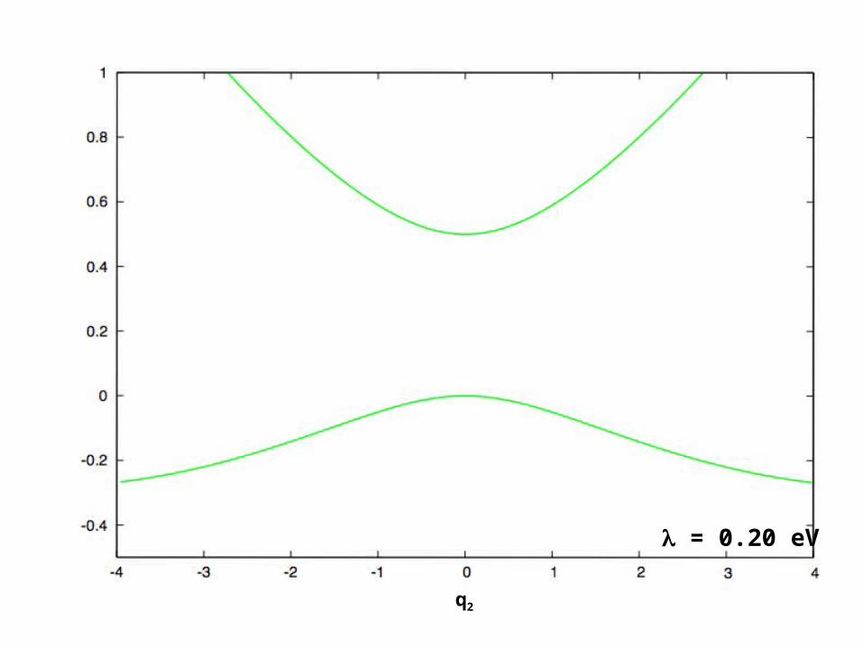
q2
= 0.20 eV

Vibronic effects on potential energy surfaces
Example: = 0.5 eV; 1 = 0.2 eV; 2 = -0.2 eV; = variable
Diabatic surfaces
A state B state

Equivalent minima
Conical Intersection
Pseudorotation transition state = 0.2 eVLowest adiabatic surface (what we calculate in quantumchemistry)

Lower adiabatic surface Upper adiabatic surface
Note that complicated (but realistic) adiabatic surfaces arise from an extremely simple model potential
Conical intersections
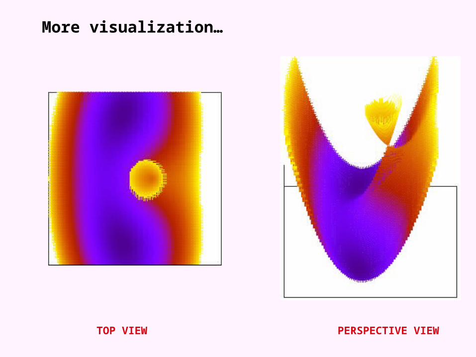
More visualization…
TOP VIEW PERSPECTIVE VIEW
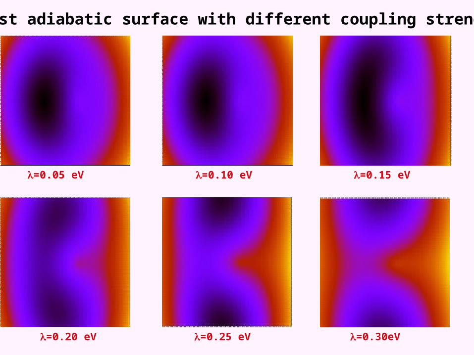
Lowest adiabatic surface with different coupling strengths
kk
=0.05 eV
=0.25 eV =0.30eV=0.20 eV
=0.15 eV=0.10 eV

Lowest adiabatic surface with different coupling strengths
kk
=0.05 eV
=0.25 eV =0.30eV=0.20 eV
=0.15 eV=0.10 eV
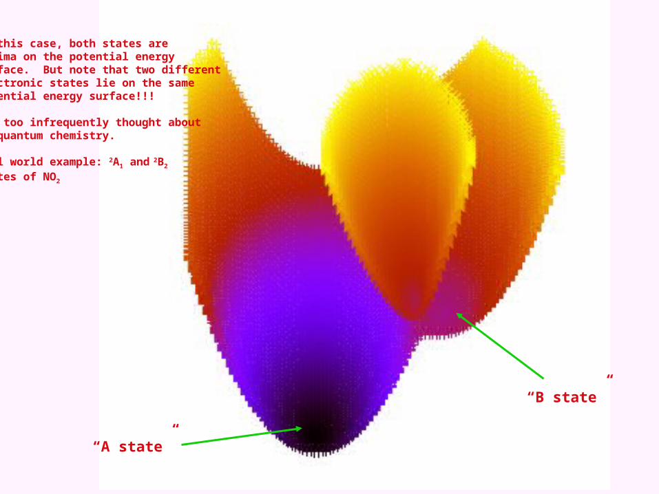
“A state”
“B state”
In this case, both states areminima on the potential energysurface. But note that two differentelectronic states lie on the samepotential energy surface!!!
Far too infrequently thought aboutin quantum chemistry.
Real world example: 2A1 and 2B2 states of NO2
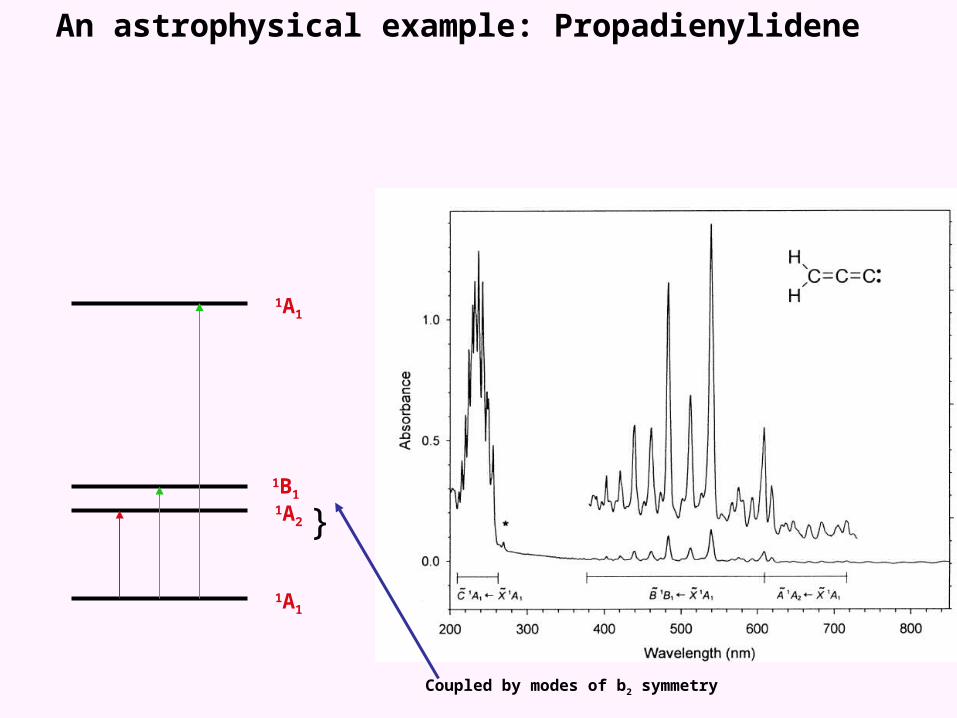
An astrophysical example: Propadienylidene
1A1
1A1
1A2
1B1
}
Coupled by modes of b2 symmetry
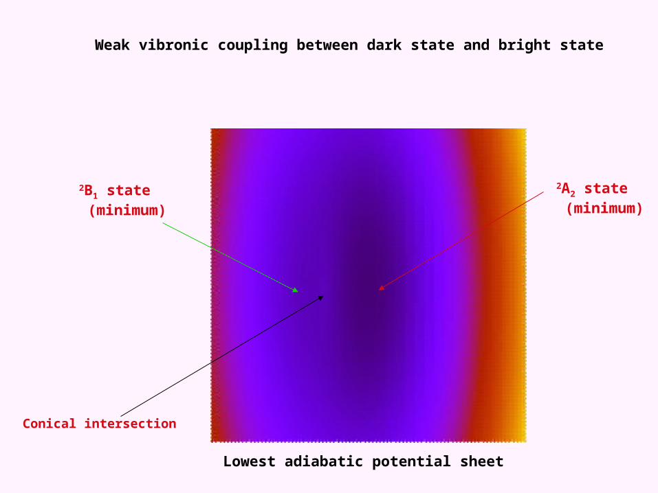
2A2 state (minimum)
2B1 state (minimum)
Conical intersection
Weak vibronic coupling between dark state and bright state
Lowest adiabatic potential sheet

Franck-Condon simulation

Franck-Condon simulation
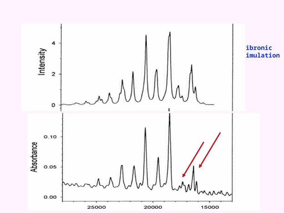
Vibronic simulation

Vibronic effects on “vibrational” energy levels
Diagonalization of complete Hamiltonian (T+V) gives vibronic energy levels
Model potential again: = 0.20 eV; = 0.5 eV; 1 = 0.2 eV; 2 = -0.2 eV
Harmonic A state frequencies from diabatic potential:
806 cm-1 (s); 323 cm-1 (a)
Harmonic A state frequencies from adiabatic potential
806 cm-1 (a); 253 cm-1 (a)
Exact vibronic levels below 1050 cm-1
250 cm-1 (n), 500 cm-1 ( 2n), 752 cm-1 ( 3n), 802 cm -1 ( s),1004 cm-1 ( 4n), 1043 cm-1 ( s+n)
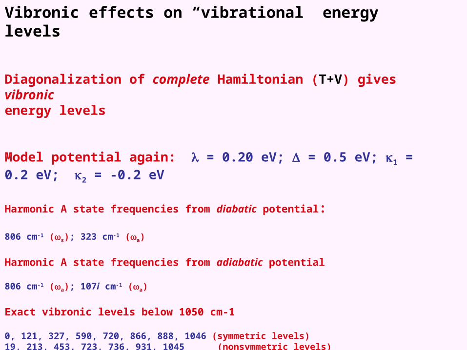
Vibronic effects on “vibrational” energy levels
Diagonalization of complete Hamiltonian (T+V) gives vibronic energy levels
Model potential again: = 0.20 eV; = 0.5 eV; 1 = 0.2 eV; 2 = -0.2 eV
Harmonic A state frequencies from diabatic potential:
806 cm-1 (s); 323 cm-1 (a)
Harmonic A state frequencies from adiabatic potential
806 cm-1 (a); 107i cm-1 (a)
Exact vibronic levels below 1050 cm-1
0, 121, 327, 590, 720, 866, 888, 1046 (symmetric levels)19, 213, 453, 723, 736, 931, 1045 (nonsymmetric levels)

Vibronic effects on potential energy surfaces
Diagonalization of potential energy (V) gives adiabatic potential energy surfaces*
n 3ns2n
Add some slides here with wavefunctions, discussion of nodes, etc.

Wavefunctions and stationary state energies
Eigenstates of system obtained by diagonalizing Hamiltonian
Given by Vibrational basis functions
= A ci i + B ci i
Diabatic electronic states

Wavefunctions and stationary state energies
Eigenstates of system obtained by diagonalizing Hamiltonian
Given by Vibrational basis functions
= A ci i + B ci i
true only if =0
= A ci I or = B ci i
“Vibrational level of electronic state A” “Vibrational level of electronic state A”
Electronic states are coupled by the off-diagonal matrix element
“Breakdown of the Born-Oppenheimer Approximation”
Diabatic electronic states

Add more slides here with wavefunctions, densities, projection onto diabatic states, etc.

The Calculation of Electronic Spectra including Vibronic Coupling
|< ’’(r,R) | | ’(r,R)>|2
‘Relative intensities given by
Energies given by
Eigenvalues of model Hamiltonian
Ground state Final state

Model system: Adiabatic perspective
Corresponding Hamiltonian verycomplicated: Potential energy matrixis diagonal but not simple (discontinuities);kinetic energy matrix is clearly not diagonal;transition dipole moment very sensitive wrtgeometry
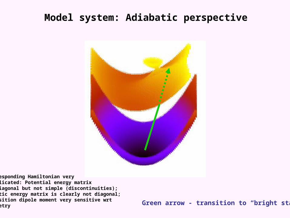
Green arrow - transition to “bright state”
Model system: Adiabatic perspective
Corresponding Hamiltonian verycomplicated: Potential energy matrixis diagonal but not simple (discontinuities);kinetic energy matrix is clearly not diagonal;transition dipole moment very sensitive wrtgeometry

Red arrow - transition to “dark state”
Green arrow - transition to “bright state”
Model system: Adiabatic perspective
Corresponding Hamiltonian verycomplicated: Potential energy matrixis diagonal but not simple (discontinuities);kinetic energy matrix is clearly not diagonal;transition dipole moment very sensitive wrtgeometry

An aside:
Traditional quantum chemistry assumes:
TA 0 VA 0 H = + 0 TB 0 VB
Vibrational energy levels calculated from the Schrödinger equations
(TA + VA) = Evib
(TB + VB) = Evib
and total (vibronic energies) given by:
Eev(A) = (VA)min + Evib
Eev(B) = (VB)min + Evib
))
) ) Adiabatic potentialenergy surfaces

T1 0 A q1 + 1/2 [1 q12 + 2 q2
2] q2
H = ( ) + ( ) 0 T2 q2 + Bq1 + 1/2 [1 q1
2 + 2 q22]
Diabatic perspective (KDC Hamiltonian) conceptually (andcomputationally a much simpler approach
Treatment:
1. Assume initial state not coupled to final states (not necessary, but a simple place to start)
2. Assume transition moments between diabatic states are constant
3. Diagonalize Hamiltonian (Lanczos recursion is best choice)
’’ = 0 000…
<0| |A> = MA
<0| |B> = MB
’ = cA0 A 000…+ cB
0 B 000… + ’[ cAi A i + cB
i B i]i
T1 0 A q1 + 1/2 [1 q12 + 2 q2
2] q2
H = ( ) + ( ) 0 T2 q2 + Bq1 + 1/2 [1 q1
2 + 2 q22]
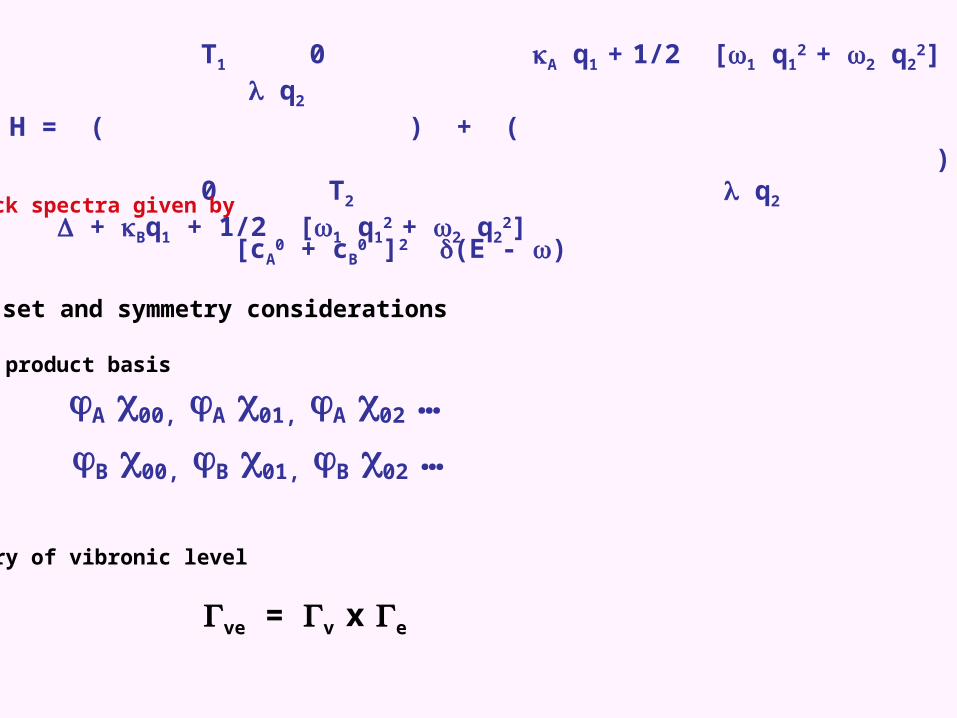
4. Stick spectra given by
Basis set and symmetry considerations
Direct product basis
A 00, A 01, A 02 …
B 00, B 01, B 02 …
Symmetry of vibronic level
ve = v x e
[cA0 + cB
0 ]2 (E - )

T1 0 A q1 + 1/2 [1 q12 + 2 q2
2] q2
H = ( ) + ( ) 0 T2 q2 + Bq1 + 1/2 [1 q1
2 + 2 q22]
4. Stick spectra given by
Basis set and symmetry considerations
Direct product basis
A 00, A 01, A 02 …
B 00, B 01, B 02 …
Symmetry of vibronic level
ve = v x e
[cA0 + cB
0 ]2 (E - )
Makes entire contribution to intensity -only ONE element of eigenvector matters

Appearance of eigenvectors - pictorial view
A
B
S
N
N
S
Franck-Condon Vibronic coupling
“vibronically allowed level”(weaker)

Appearance of eigenvectors - pictorial view
A
B
S
N
N
S
Franck-Condon Vibronic coupling
“vibronically allowed level”(stronger)
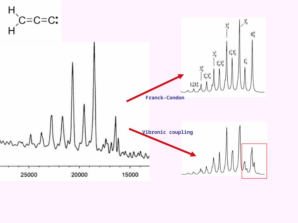
Franck-Condon
Vibronic coupling
Application to NO2 photoelectron spectra: The nuts and bolts
1. Choose a quantum-chemical method

Application to NO2 photoelectron spectra: The nuts and bolts
1. Choose a quantum-chemical method EOMIP-CCSD with cc-pVDZ basis

Application to NO2 photoelectron spectra: The nuts and bolts
1. Choose a quantum-chemical method EOMIP-CCSD with cc-pVDZ basis
2. Choose a reference state and coordinate system

Application to NO2 photoelectron spectra: The nuts and bolts
1. Choose a quantum-chemical method EOMIP-CCSD with cc-pVDZ basis
2. Choose a reference state and coordinate system Anion and its DNCs

Application to NO2 photoelectron spectra: The nuts and bolts
1. Choose a quantum-chemical method EOMIP-CCSD with cc-pVDZ basis
2. Choose a reference state and coordinate system Anion and its DNCs
• Quantum-chemical calculations begin!
A. Optimize geometry and get DNCs for NO2-
no2 anion - optimized geometryON 1 R*O 2 R* 1 A*
R = 1.253566124038471A = 116.244941874549653
*CRAPS(CALC=CCSD,BASIS=PVDZCHARGE=-1,CC_CONV=9,LINEQ_CONV=9,MEM=100000000)
Input for geometryoptimization

Output from geometryoptimization
Forces are in hartree/bohr and hartree/radian.
Parameter values are in Angstroms and degrees.-------------------------------------------------------------------------- Parameter dV/dR Step Rold Rnew-------------------------------------------------------------------------- R 0.0000008145 -0.0000005378 1.2629668229 1.2629662851 A 0.0000013123 -0.0001124564 115.9925199928 115.9924075364-------------------------------------------------------------------------- Minimum force: 0.000000815 / RMS force: 0.000001092
no2 anion - optimized geometryON 1 RO 2 R 1 A
R = 1.262966285109282A = 115.992407536378849
*CRAPS(CALC=CCSD,BASIS=PVDZ,VIB=EXACTCHARGE=-1,CC_CONV=9,LINEQ_CONV=9,MEM=100000000)
Input for harmonic Frequency calcualtion
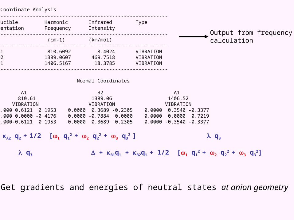
Output from frequencycalculation
Normal Coordinate Analysis
---------------------------------------------------------------- Irreducible Harmonic Infrared Type Representation Frequency Intensity ---------------------------------------------------------------- (cm-1) (km/mol) ---------------------------------------------------------------- A1 810.6092 8.4024 VIBRATION B2 1389.0607 469.7518 VIBRATION A1 1406.5167 18.3785 VIBRATION ---------------------------------------------------------------- Normal Coordinates A1 B2 A1 810.61 1389.06 1406.52 VIBRATION VIBRATION VIBRATION O 0.000 0.6121 0.1953 0.0000 0.3689 -0.2305 0.0000 0.3540 -0.3377 N 0.000 0.0000 -0.4176 0.0000 -0.7884 0.0000 0.0000 0.0000 0.7219 O 0.000-0.6121 0.1953 0.0000 0.3689 0.2305 0.0000 -0.3540 -0.3377
B. Get gradients and energies of neutral states at anion geometry
T A 0 A1 q1 + A2 q2 + 1/2 [1 q12 + 2 q2
2 + 3 q32 ] q3
H = ( ) + ( ) 0 TB q3 + B1q1 + B2q1 + 1/2 [1 q1
2 + 2 q22 + 3 q3
2]
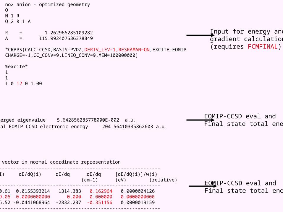
Input for energy andgradient calculation(requires FCMFINAL)
no2 anion - optimized geometryON 1 RO 2 R 1 A
R = 1.262966285109282A = 115.992407536378849
*CRAPS(CALC=CCSD,BASIS=PVDZ,DERIV_LEV=1,RESRAMAN=ON,EXCITE=EOMIPCHARGE=-1,CC_CONV=9,LINEQ_CONV=9,MEM=100000000)
%excite*111 0 12 0 1.00
Gradient vector in normal coordinate representation
---------------------------------------------------------- i W(I) dE/dQ(i) dE/dq dE/dq [dE/dQ(i)]/w(i) (cm-1) (eV) (relative) ---------------------------------------------------------- 7 810.61 0.0155393214 1314.383 0.162964 0.0000004126 8 1389.06 0.0000000000 0.000 0.000000 0.0000000000 9 1406.52 -0.0441068964 -2832.237 -0.351156 0.0000019159 ----------------------------------------------------------
Converged eigenvalue: 5.642856285778000E-002 a.u.
Total EOMIP-CCSD electronic energy -204.56410335862603 a.u.
EOMIP-CCSD eval andFinal state total energy
EOMIP-CCSD eval andFinal state total energy

T A 0 A1 q1 + A2 q2 + 1/2 [1 q12 + 2 q2
2 + 3 q32 ] q3
H = ( ) + ( ) 0 TB q3 + B1q1 + B2q2 + 1/2 [1 q1
2 + 2 q22 + 3 q3
2]
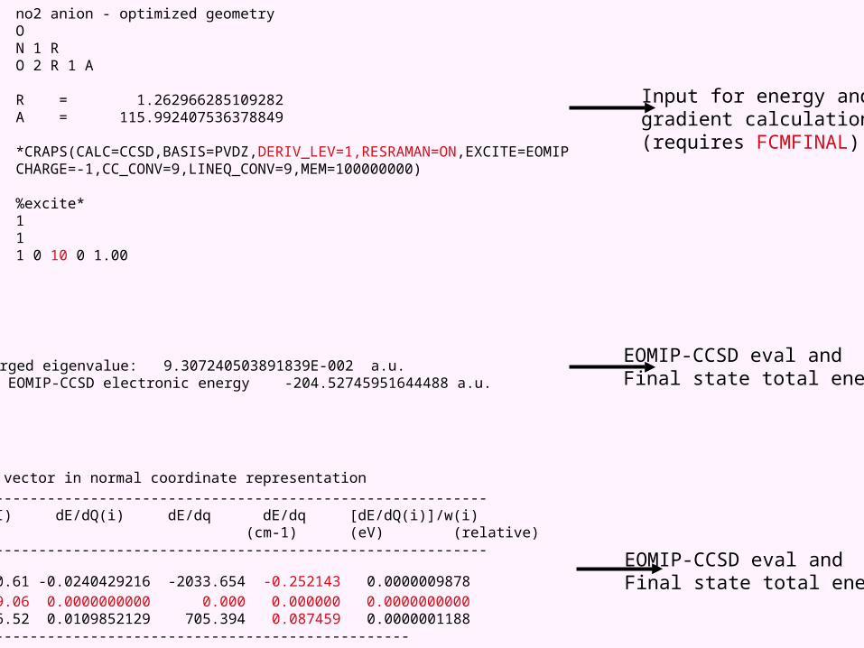
Input for energy andgradient calculation(requires FCMFINAL)
no2 anion - optimized geometryON 1 RO 2 R 1 A
R = 1.262966285109282A = 115.992407536378849
*CRAPS(CALC=CCSD,BASIS=PVDZ,DERIV_LEV=1,RESRAMAN=ON,EXCITE=EOMIPCHARGE=-1,CC_CONV=9,LINEQ_CONV=9,MEM=100000000)
%excite*111 0 10 0 1.00
Gradient vector in normal coordinate representation
---------------------------------------------------------- i W(I) dE/dQ(i) dE/dq dE/dq [dE/dQ(i)]/w(i) (cm-1) (eV) (relative) ----------------------------------------------------------
7 810.61 -0.0240429216 -2033.654 -0.252143 0.0000009878
8 1389.06 0.0000000000 0.000 0.000000 0.0000000000 9 1406.52 0.0109852129 705.394 0.087459 0.0000001188----------------------------------------------------------
Converged eigenvalue: 9.307240503891839E-002 a.u.Total EOMIP-CCSD electronic energy -204.52745951644488 a.u.
EOMIP-CCSD eval andFinal state total energy
EOMIP-CCSD eval andFinal state total energy

T A 0 A1 q1 + A2 q2 + 1/2 [1 q12 + 2 q2
2 + 3 q32 ] q3
H = ( ) + ( ) 0 TB q3 + B1q1 + B2q2 + 1/2 [1 q1
2 + 2 q22 + 3 q3
2]

T A 0 A1 q1 + A2 q2 + 1/2 [1 q12 + 2 q2
2 + 3 q32 ] q3
H = ( ) + ( ) 0 TB q3 + B1q1 + B2q1 + 1/2 [1 q1
2 + 2 q22 + 3 q3
2]
What do we do aboutthis????? HamiltonianIs in “diabatic” basis, andq.c. calculates adiabatic energies

T A 0 A1 q1 + A2 q2 + 1/2 [1 q12 + 2 q2
2 + 3 q32 ] q3
H = ( ) + ( ) 0 TB q3 + B1q1 + B2q1 + 1/2 [1 q1
2 + 2 q22 + 3 q3
2]
What do we do aboutthis????? HamiltonianIs in “diabatic” basis, andq.c. calculates adiabatic energies
… transform model Hamiltonian back to adiabatic basis!
T A TAB A1 q1 + A2 q2 + 1/2 [f1 q12 + f2 q2
2 + fA3 q32 ] 0
H = ( ) + ( ) TAB TB 0 + B1q1 + B2q1 + 1/2 [f1 q1
2 + f2 q22 + fB3 q3
2]
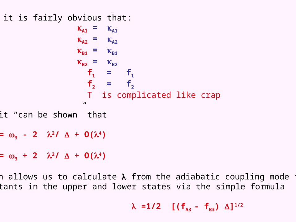
Now, it is fairly obvious that: A1 = A1 A2 = A2 B1 = B1 B2 = B2 f1 = f1 f2 = f2
T is complicated like crap
and it “can be shown” that
fA3 = 3 - 2 2/ + O(4)
fB3 = 3 + 2 2/ + O(4)
which allows us to calculate from the adiabatic coupling mode forceconstants in the upper and lower states via the simple formula
=1/2 [(fA3 - fB3) ]1/2
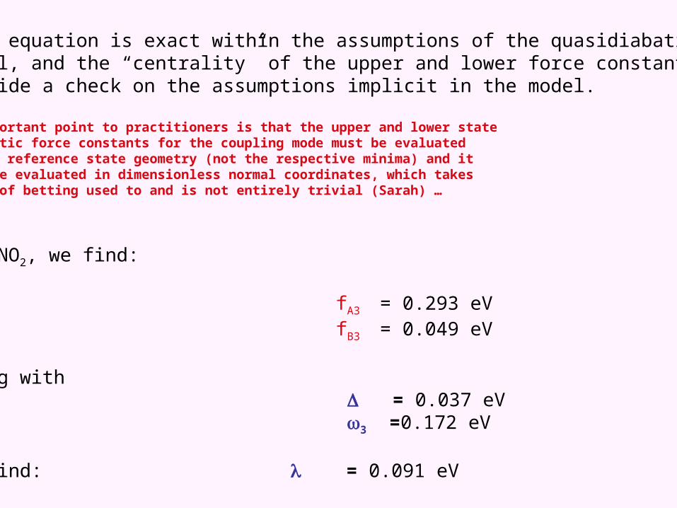
This equation is exact within the assumptions of the quasidiabaticmodel, and the “centrality” of the upper and lower force constantsprovide a check on the assumptions implicit in the model.
An important point to practitioners is that the upper and lower stateadiabatic force constants for the coupling mode must be evaluated at the reference state geometry (not the respective minima) and itmust be evaluated in dimensionless normal coordinates, which takesa bit of betting used to and is not entirely trivial (Sarah) …
For NO2, we find:
fA3 = 0.293 eV fB3 = 0.049 eV
along with = 0.037 eV 3 =0.172 eV
We find: = 0.091 eV
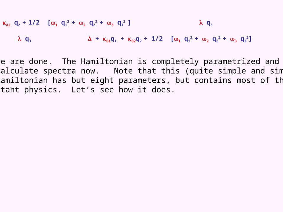
T A 0 A1 q1 + A2 q2 + 1/2 [1 q12 + 2 q2
2 + 3 q32 ] q3
H = ( ) + ( ) 0 TB q3 + B1q1 + B2q2 + 1/2 [1 q1
2 + 2 q22 + 3 q3
2]
And we are done. The Hamiltonian is completely parametrized and wecan calculate spectra now. Note that this (quite simple and simplest)KDC Hamiltonian has but eight parameters, but contains most of the important physics. Let’s see how it does.