Atmos. Meas. Tech., 11, 4725–4736, 2018https://doi.org/10.5194/amt-11-4725-2018© Author(s) 2018. This work is distributed underthe Creative Commons Attribution 4.0 License.

Calculating uncertainty for the RICE ice core continuous flowanalysis water isotope recordElizabeth D. Keller1, W. Troy Baisden1,a, Nancy A. N. Bertler1,2, B. Daniel Emanuelsson1,2, Silvia Canessa1, andAndy Phillips1

1National Isotope Centre, GNS Science, Lower Hutt, New Zealand2Antarctic Research Centre, Victoria University of Wellington, Wellington, New Zealandanow at: Environmental Research Institute, University of Waikato, Hamilton, New Zealand

Correspondence: Elizabeth D. Keller (l.keller@gns.cri.nz)

Received: 27 October 2017 – Discussion started: 9 January 2018Revised: 21 July 2018 – Accepted: 25 July 2018 – Published: 13 August 2018

Abstract. We describe a systematic approach to the calibra-tion and uncertainty estimation of a high-resolution contin-uous flow analysis (CFA) water isotope (δ2H, δ18O) recordfrom the Roosevelt Island Climate Evolution (RICE) Antarc-tic ice core. Our method establishes robust uncertainty esti-mates for CFA δ2H and δ18O measurements, comparable tothose reported for discrete sample δ2H and δ18O analysis.Data were calibrated using a time-weighted two-point lin-ear calibration with two standards measured both before andafter continuously melting 3 or 4 m of ice core. The errorat each data point was calculated as the quadrature sum ofthree factors: Allan variance error, scatter over our averag-ing interval (error of the variance) and calibration error (er-ror of the mean). Final mean total uncertainty for the entirerecord is δ2H= 0.74‰ and δ18O= 0.21‰. Uncertaintiesvary through the data set and were exacerbated by a rangeof factors, which typically could not be isolated due to therequirements of the multi-instrument CFA campaign. Thesefactors likely occurred in combination and included ice qual-ity, ice breaks, upstream equipment failure, contaminationwith drill fluid and leaks or valve degradation. We demon-strate that our methodology for documenting uncertainty waseffective across periods of uneven system performance anddelivered a significant achievement in the precision of high-resolution CFA water isotope measurements.

1 Introduction

Stable water isotopes (δ2H, δ18O) are a fundamental part ofice core studies. They are particularly important as a tem-perature proxy (Dansgaard, 1964; Epstein et al., 1963) andare a key component in establishing the age–depth scale andchronology of ice cores (NGRIP Members, 2004; Vinther etal., 2006; Winstrup et al., 2017). They also provide other in-formation about climate, including accumulation rates, pre-cipitation source region, atmospheric circulation and air masstransport, and sea ice extent (e.g. Küttel et al., 2012; Sinclairet al., 2013; Steig et al., 2013; Bertler et al., 2018; Emanuels-son et al., 2018).

Historically, water isotopes from ice cores were anal-ysed as a set of discrete water samples using isotope ratiomass spectrometry (Dansgaard, 1964). Recent advances inlaser absorption spectrometry have allowed continuous flowanalysis (CFA) to become common in ice core studies andare an essential measurement technique for obtaining high-resolution climate records (e.g. Kaufmann et al., 2008; Gki-nis et al., 2011; Kurita et al., 2012; Emanuelsson et al., 2015;Jones et al., 2017). However, the simultaneous operation ofseven measurement systems (Winstrup et al., 2017; Pyneet al., 2018) and the continuous nature of CFA pose chal-lenges for calibration and uncertainty estimation. Becauseof the size and resolution of CFA ice core data sets andthe relatively new application of laser spectroscopy to icecores, few established methods exist for calculating point-by-point uncertainty throughout measurements. Building onprevious studies (e.g. Gkinis et al., 2011; Kurita et al., 2012;Emanuelsson et al., 2015), we have developed a systematic

Published by Copernicus Publications on behalf of the European Geosciences Union.

4726 E. D. Keller et al.: RICE CFA water isotope record uncertainty

approach to calibration and error calculation that allows forunique uncertainty estimates at each data point in a CFA wa-ter isotope record. In this study, we report our methodologyfor the calibration and calculation of uncertainty and demon-strate the application of the method on the Roosevelt IslandClimate Evolution (RICE) ice core δ2H and δ18O data set.

The RICE collaboration retrieved a 760 m ice core fromthe north-eastern edge of the Ross Ice Shelf over RooseveltIsland in Antarctica (79.39◦ S, 161.46◦W, 550 m a.s.l) duringthe austral summer 2011–2012 and 2012–2013 field seasons(Bertler et al., 2018). The RICE ice core provides a valu-able record of a high snow accumulation site in coastal WestAntarctica with annual or sub-annual resolution at the up-per depths, representing the late Holocene. The climate re-construction at the RICE site for the last 2700 years usingthe CFA water isotope record is available in a separate pub-lication (Bertler et al., 2018). In addition to the value in themethodology itself, this paper provides confidence in the pre-cision of the RICE data set and the climatic interpretationon annual and sub-annual timescales. This method can beapplied to other high-resolution CFA ice core water isotoperecords in the future and may be suitable for other continuouswater isotope measurement applications.

This paper is structured as follows: in Sect. 2, we give anoverview of our data processing and data quality control pro-cedure. We also detail our methods for calibrating the isotopedata and calculating the uncertainty for each data point. Sec-tion 3 contains the resulting estimates for each component ofthe total error of our data set and an analysis of the differentsources of error. We conclude in Sect. 4 with a summary andrecommendations for future CFA measurement campaigns.

2 Methods

The abundance of the rare isotope in a sample is convention-ally reported in delta notation, defined as

δ =

(Rsample

Rstandard− 1,

)(1)

where R is 18O/16O or 2H/1H for water stable isotopes(Coplen, 2011). Results in this paper are reported as δ valuesin parts per thousand (‰), normalized to the internationalstandard Vienna Standard Mean Ocean Water and StandardLight Antarctic Precipitation (VSMOW-SLAP) scale (Gon-fiantini, 1978).

2.1 Melting and data processing

Cores were melted and processed at the Ice Core Labora-tory at the GNS National Isotope Centre in Lower Hutt, NewZealand. There were two separate melting campaigns, one inJune–July 2013, in which the top 500 m were melted, and theother in June–July 2014, in which the remaining 260 m (500–760 m) were melted (Pyne et al., 2018). There were several

important differences between the 2 years in the CFA set-up(Emanuelsson et al., 2015; Pyne et al., 2018), which necessi-tated that the data from each melting campaign be processedseparately. These differences are noted where they are rele-vant to the calibration and uncertainty calculations; some fac-tors were calculated individually for each melting campaignand applied only to the data from that campaign.

The ice was cut into 1 m segments and melted at a con-trolled rate of approximately 3 cm min−1, producing a liquidflow rate of ∼ 16.8mLmin−1 (Pyne et al., 2018). The melt-ing set-up is based on Bigler et al. (2011) and is discussed inmore detail in Emanuelsson et al. (2015), Pyne et al. (2018)and Winstrup et al. (2017). Briefly, the cores were placed ver-tically on a gold-coated copper melting plate and were al-lowed to melt continuously under gravitational pull. The wa-ter from the clean, inner part of the core was drawn from thecentre of the melt head and pumped to instruments for CFAof stable isotopes, methane, black carbon, insoluble dust par-ticles, calcium, pH and conductivity and discrete samples formajor ion and trace element analyses. The water from theouter part of the core was saved in vials for discrete stableand radioactive isotope analysis. Either three or four 1 m coresegments were stacked on top of each other and melted with-out interruption (referred to here as a “stack”). At least onecalibration cycle of three water standards was run betweeneach stack. An optical encoder that rested on top of the corestack recorded the vertical distance displacement as the coremelted. This displacement was translated into depth in mil-limetres and, along with the melting rate and other system in-formation, was written to a log file every 1 s using LabVIEWsoftware (National Instruments). These log files were usedto align all CFA instrument data to the depth scale. Breaksin the ice were measured and recorded to 1.0 mm precisionbefore melting. Any ice that was cut out and removed wasrecorded as a gap in the depth scale. The raw data files wereprocessed using a graphical user interface (GUI) and a semi-automated script written in Matlab (Matlab Release 2012b,The MathWorks, Inc., Natick, Massachusetts, United States).Occasionally, poor-quality ice (i.e. ice containing fracturesand slanted breaks) caused the upper part of the stack to stickto the sides of the core holder; the depth encoder failed toregister any change in depth for a time, while the base ofthe stack continued to melt. These intervals required linearinterpolation (assuming a constant melt rate) and introduceda small amount of uncertainty (Pyne et al., 2018). This oc-curred more frequently deeper in the core in the brittle icezone (below 500 m). Given that the melt rate was fairly con-stant throughout the campaign, the error introduced in thedepth assignment was negligible. More details of the dataprocessing are available in Pyne et al. (2018).

Water isotope values (δ2H, δ18O) were measured usingCFA with a water vapour isotope analyser (WVIA) using off-axis integrated cavity output spectroscopy (OA-ICOS; Baeret al., 2002) and a modified Water Vapour Isotopic Stan-dard Source (WVISS) calibration unit (manufactured by Los

Atmos. Meas. Tech., 11, 4725–4736, 2018 www.atmos-meas-tech.net/11/4725/2018/

E. D. Keller et al.: RICE CFA water isotope record uncertainty 4727

Gatos Research, LGR). This system is described in detail inEmanuelsson et al. (2015). The 2013 and 2014 set-ups werelargely the same but differed in the construction of the va-porizer and the delivery of the mixed vapour to the isotopeanalyser. In 2014, the heating element of the vaporizer wasmodified, and a higher sample flow was delivered directly tothe IWA through an open split (Emanuelsson et al., 2015).Data were recorded in an output file at a rate of 2 Hz (0.5 s)in 2013 and at 1 Hz (1.0 s) for the remaining 260 m in 2014.The change in the recording rate of the isotope data in 2014was made to match the rate at which the depth was recordedin both years (1 Hz). Note that this was not a change in theinstrument’s internal data acquisition rate, only in the rate ofoutput aggregation.

The campaigns altogether required processing and align-ment of over 5 million raw data points. Depth alignmentacross multiple measurement systems is a key issue for icecore campaigns and a fundamental requirement for produc-ing an age chronology (Winstrup et al., 2017). The interpre-tation and identification of key events in the climate historythus depend on accurate depth alignment. This is particularlyimportant deeper in the core, where a misalignment of a fewcentimetres could equate to hundreds or even thousands ofyears (Lee et al., 2018). Alignment of the isotope data to thedepth scale is based on the time lag between the depth logfile and the WVIA instrument output. The time lag was de-termined with an automated algorithm to detect the end ofthe calibration cycle and the beginning of the ice core meltstream using the abrupt increase in the change in numericderivatives of adjacent data points. The calculated time lagsduring each measurement campaign averaged 418 s in 2013and 156 s in 2014 but varied slightly from day to day by 10–20 s. (The lag was shorter in 2014 due to the reduction inlength of tubing between the melter and WVIA. Variationsoccurred from the periodic replacement of the tubing.) Therewere a few occasions of equipment failure where manualdepth alignment was necessary. Poor ice quality also affectedthe accuracy of the depth log files, as mentioned above (Pyneet al., 2018). The precise quantification of the uncertainty in-troduced from the depth assignment is beyond the scope ofthis paper; based on the variation in time lags, we estimatethat, at most, it is of the order of 1–10 mm.

2.2 Data quality control

We applied several basic selection criteria to identify andeliminate poor-quality data from the raw δ2H and δ18O dataset. The two main reasons for data removal were (1) changesin the water vapour concentration (H2O ppm) in the LGRanalyser, and (2) the finite response time of the analyser andthe transitional period when switching between water stan-dards from the calibration cycle and RICE ice core meltwa-ter (which by design had very different isotopic values). Inaddition, some gaps were introduced as a result of cuttingthe core into 1 m segments and the fractures in the ice that

Figure 1. An example of the raw data from a full day of ice melt-ing and calibration cycles (2–3 July 2014): (a) δ2H, (b) δ18O and(c) water vapour mixing ratio. Isotope data that were removed be-cause of water concentration anomalies are marked in red in (a, b)panels.

occurred during the drilling, recovery and handling process(Pyne et al., 2018).

The isotope ratio is dependent on water vapour concen-tration in the analyser (Sturm and Knohl, 2010; Kurita etal., 2012). To minimize the need to correct the data forthis, the concentration in the analyser was kept as closeto 20 000 ppm as possible. This value was monitored andrecorded at the same frequency as the isotope data. For themost part this concentration was stable, but fluctuations andsudden changes did sometimes occur (for example, when airbubbles passed through the line). We removed data when thedifference between the H2O ppm moving average over theshort-term system response time of ∼ 60s and over a longer-term, stable time of∼ 200s was greater than the standard de-viation of the short-term average (Emanuelsson et al., 2015):∣∣avgs − avgl

∣∣> σs, where σs is the standard deviation of theshort-term average. In addition, data were removed if the wa-ter vapour concentration fell below 15 000 ppm for an ex-tended period. This filtering removed the need to further cor-rect for variations in water vapour concentration in the record(Emanuelsson et al., 2015). Figure 1 shows a typical day ofraw data, including both RICE ice core stacks and calibrationcycles. Data marked in red were removed using these crite-ria. The majority of these points occur during the switch fromone water standard to another in the calibration cycle and donot affect the data from the ice core itself. The percentage ofdata removed using these criteria was 0.4 % of the total.

It was also necessary to remove some data points at thebeginning and end of every stack during the transition periodbetween the Milli Q (18.2 M�) laboratory water standardand ice core. This transition is illustrated in Fig. 2. The MilliQ standard is composed of local de-ionized water and has anisotopic value much greater than the RICE ice core (Table 1).

www.atmos-meas-tech.net/11/4725/2018/ Atmos. Meas. Tech., 11, 4725–4736, 2018

4728 E. D. Keller et al.: RICE CFA water isotope record uncertainty

Figure 2. A selected example section of δ2H vs. depth. The datamarked in red represent the transitions between the Milli Q standardand ice core at the boundaries of each 3 m stack. These data points(and other poor quality data) were removed from the final data set.

Milli Q was run immediately before and after each stack, andthere is a period of instrumental adjustment and mixing whenswitching between them due to memory effects and the finiteresponse time of the spectrometer (see Emanuelsson et al.,2015 for a full discussion). To ensure that the data are notinfluenced by mixing at the beginning and end of the stackwhile including as much data as possible, we calculated thenumerical derivative (or the rate of change) between consec-utive δ2H data points during the transition until the derivativefalls below a threshold; all points prior are then excluded.The same process is performed at the end of the stack in re-verse. The threshold was found empirically and is differentin 2013 and 2014 because of the difference in the responsetimes of the two set-ups and the precision of the data. Datawere inspected manually for cases where the algorithm wasinadequate. Approximately 2–5 cm at the beginning and endof every stack was removed using this condition. These ap-pear as gaps in the depth of the final data set. There were alsoa few occasions when melting was interrupted due to equip-ment failure, and Milli Q was run through the system untilmelting could resume; these periods were removed using thesame procedure. A typical stack showing a portion of dataremoved is shown in Fig. 2 (δ2H vs. depth). The fraction oftotal data removed was 5.4 %. This resulted in short data gapsof 2–5 cm every 3 or 4 m.

The entire data set was manually inspected for any otherregions of poor quality, and points that visibly fell outside thenormal range or were affected by known instrument prob-lems were removed. This only applied to a few isolated sec-tions of data and was a very small portion (< 0.1 %) of thetotal.

Table 1. Accepted values (VSMOW-SLAP scale) for water stan-dards used for calibrations in per mil (‰).

Water standard δ18O (‰) δ2H (‰)

Milli Q −5.89± 0.05 −34.85± 0.18WS1-13 −10.84± 0.10 −74.15± 0.94WS1-14 −10.83± 0.05 −74.85± 0.18RICE-13 −22.54± 0.05 −175.02± 0.19RICE-14 −22.27± 0.05 −173.06± 0.24ITASE-13 −37.39± 0.05 −299.66± 0.18ITASE-14 −36.91± 0.08 −295.49± 0.52

2.3 Calibration

It is necessary in laser spectroscopy to normalize the iso-topic values to the VSMOW-SLAP scale and to correct forinstrumental drift. To accomplish this, we used a two-pointlinear calibration method (Paul et al., 2007; Kurita et al.,2012). Before and after each ice core stack, we ran calibra-tion sequences consisting of four laboratory water standards:Milli Q, Working Standard 1 (WS1), RICE snow (RICE) andUS International Trans-Antarctic Scientific Expedition WestAntarctic snow (ITASE). An example of a calibration cycle isshown in Fig. 3. Assigned or “true” values for these standardsmeasured against the VSMOW-2-SLAP-2 scale are listed inTable 1. Each batch of working standards was calibratedto the International Atomic Energy Agency (IAEA) pri-mary standards, VSMOW-2 (δ18O= 0.0‰; δ2H= 0.0‰),SLAP-2 (δ18O=−55.50‰; δ2H=−427.5‰) and GISP(δ18O=−24.76‰; δ2H=−189.5‰), using three interme-diate, secondary standards, INS11 (δ18O=−0.37‰; δ2H=−4.2‰), CM1 (δ18O=−16.91‰; δ2H=−129.51‰) andSM1 (δ18O=−28.79‰; δ2H=−225.4‰).

We note that there is a difference in the assigned valuesfor RICE and ITASE between 2013 and 2014. We have de-noted them RICE-13, RICE-14, ITASE-13 and ITASE-14 inTable 1 to indicate that these standards were prepared andstored in different batches in each year, from water sourcesthat had not been treated as standards or homogenized, andthus are slightly different in composition. We emphasize herethat our standards are local working standards, selected ormixed by our laboratory to match the isotope ratios of thesample (melt stream). It is not unexpected that their isotopicvalue will change between batches during long measurementcampaigns, as it is not practical to prepare and store all of thematerial in one batch.

Part of the difference in assigned values might be at-tributed to the difference in measurement systems. The as-signed values for the 2013 calibrations were determined us-ing discrete laser absorption spectroscopy measurements onan Isotope Water Analyzer (IWA) 35EP system. In 2014, ourinstrument was upgraded with a second laser to IWA-45EP,and the 2014 calibrations utilize values from standards mea-sured continuously with this system. We were regrettably

Atmos. Meas. Tech., 11, 4725–4736, 2018 www.atmos-meas-tech.net/11/4725/2018/

E. D. Keller et al.: RICE CFA water isotope record uncertainty 4729

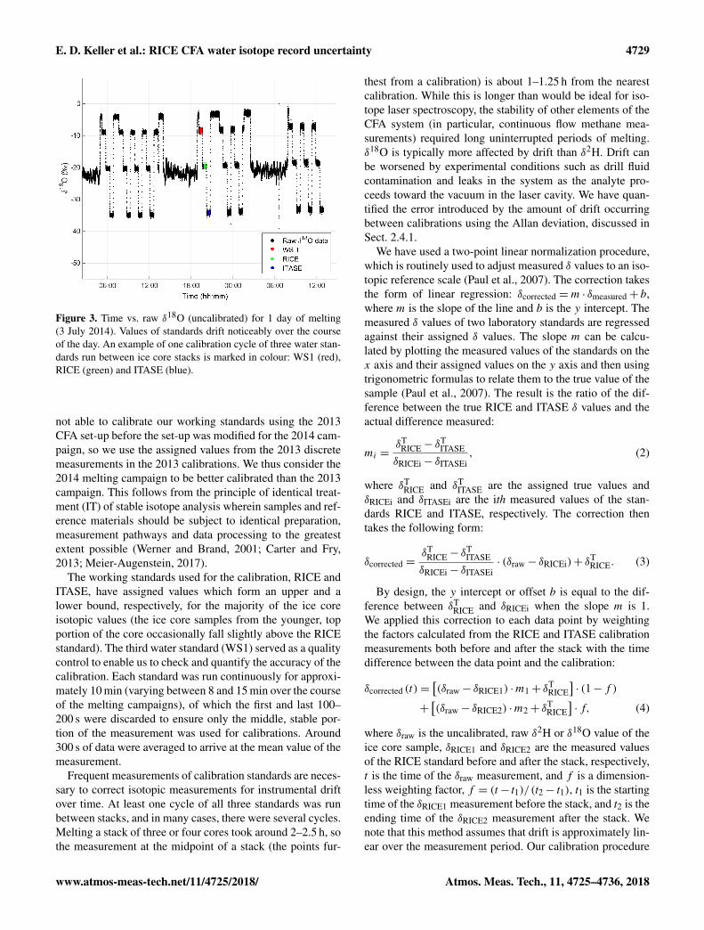
Figure 3. Time vs. raw δ18O (uncalibrated) for 1 day of melting(3 July 2014). Values of standards drift noticeably over the courseof the day. An example of one calibration cycle of three water stan-dards run between ice core stacks is marked in colour: WS1 (red),RICE (green) and ITASE (blue).

not able to calibrate our working standards using the 2013CFA set-up before the set-up was modified for the 2014 cam-paign, so we use the assigned values from the 2013 discretemeasurements in the 2013 calibrations. We thus consider the2014 melting campaign to be better calibrated than the 2013campaign. This follows from the principle of identical treat-ment (IT) of stable isotope analysis wherein samples and ref-erence materials should be subject to identical preparation,measurement pathways and data processing to the greatestextent possible (Werner and Brand, 2001; Carter and Fry,2013; Meier-Augenstein, 2017).

The working standards used for the calibration, RICE andITASE, have assigned values which form an upper and alower bound, respectively, for the majority of the ice coreisotopic values (the ice core samples from the younger, topportion of the core occasionally fall slightly above the RICEstandard). The third water standard (WS1) served as a qualitycontrol to enable us to check and quantify the accuracy of thecalibration. Each standard was run continuously for approxi-mately 10 min (varying between 8 and 15 min over the courseof the melting campaigns), of which the first and last 100–200 s were discarded to ensure only the middle, stable por-tion of the measurement was used for calibrations. Around300 s of data were averaged to arrive at the mean value of themeasurement.

Frequent measurements of calibration standards are neces-sary to correct isotopic measurements for instrumental driftover time. At least one cycle of all three standards was runbetween stacks, and in many cases, there were several cycles.Melting a stack of three or four cores took around 2–2.5 h, sothe measurement at the midpoint of a stack (the points fur-

thest from a calibration) is about 1–1.25 h from the nearestcalibration. While this is longer than would be ideal for iso-tope laser spectroscopy, the stability of other elements of theCFA system (in particular, continuous flow methane mea-surements) required long uninterrupted periods of melting.δ18O is typically more affected by drift than δ2H. Drift canbe worsened by experimental conditions such as drill fluidcontamination and leaks in the system as the analyte pro-ceeds toward the vacuum in the laser cavity. We have quan-tified the error introduced by the amount of drift occurringbetween calibrations using the Allan deviation, discussed inSect. 2.4.1.

We have used a two-point linear normalization procedure,which is routinely used to adjust measured δ values to an iso-topic reference scale (Paul et al., 2007). The correction takesthe form of linear regression: δcorrected =m · δmeasured+ b,where m is the slope of the line and b is the y intercept. Themeasured δ values of two laboratory standards are regressedagainst their assigned δ values. The slope m can be calcu-lated by plotting the measured values of the standards on thex axis and their assigned values on the y axis and then usingtrigonometric formulas to relate them to the true value of thesample (Paul et al., 2007). The result is the ratio of the dif-ference between the true RICE and ITASE δ values and theactual difference measured:

mi =δT

RICE− δTITASE

δRICEi− δITASEi, (2)

where δTRICE and δT

ITASE are the assigned true values andδRICEi and δITASEi are the ith measured values of the stan-dards RICE and ITASE, respectively. The correction thentakes the following form:

δcorrected =δT

RICE− δTITASE

δRICEi− δITASEi· (δraw− δRICEi)+ δ

TRICE. (3)

By design, the y intercept or offset b is equal to the dif-ference between δT

RICE and δRICEi when the slope m is 1.We applied this correction to each data point by weightingthe factors calculated from the RICE and ITASE calibrationmeasurements both before and after the stack with the timedifference between the data point and the calibration:

δcorrected (t)=[(δraw− δRICE1) ·m1+ δ

TRICE

]· (1− f )

+[(δraw− δRICE2) ·m2+ δ

TRICE

]· f, (4)

where δraw is the uncalibrated, raw δ2H or δ18O value of theice core sample, δRICE1 and δRICE2 are the measured valuesof the RICE standard before and after the stack, respectively,t is the time of the δraw measurement, and f is a dimension-less weighting factor, f = (t− t1)/(t2− t1), t1 is the startingtime of the δRICE1 measurement before the stack, and t2 is theending time of the δRICE2 measurement after the stack. Wenote that this method assumes that drift is approximately lin-ear over the measurement period. Our calibration procedure

www.atmos-meas-tech.net/11/4725/2018/ Atmos. Meas. Tech., 11, 4725–4736, 2018

4730 E. D. Keller et al.: RICE CFA water isotope record uncertainty

was validated by comparison with discrete measurements inEmanuelsson et al. (2015). The values of the slope correc-tions and the RICE and ITASE raw measurements used tocalibrate the data in each year are shown in Figs. S2–S4 inthe Supplement; mean values and standard deviations are inTable S1 in the Supplement.

2.4 Uncertainty calculation

We identified three main sources of uncertainty in our mea-surements: (i) the Allan variance error (a measure of our abil-ity to correct for drift, a systematic source of uncertainty dueto instrumental instability), (ii) the scatter or noise in the dataover our chosen averaging interval, and (iii) a general calibra-tion error relating to the overall accuracy of our calibration.Our three error factors can be formally categorized as fol-lows:

i. Allan variance error is the systematic error or bias dueto our imperfect ability to correct for drift;

ii. scatter error is the error of the variance, precision or ran-dom variation of replicate measurements;

iii. calibration error is the error of the mean or trueness.

The last two can be quantified with general analytical ex-pressions (Kirchner, 2001). Systematic error does not have ageneral analytical form; isotopic drift is fortunately amenableto correction, but the method is imperfect.

We assume that the three error factors are uncorrelated to alarge degree. This is supported by the general framework thatwe have used (Kirchner, 2001; Analytical Methods Commit-tee, 2003) and the actual errors calculated at each data point(R2 < 0.05 in each year for both isotopes). In practice it is im-possible for all error factors to be completely uncorrelated,as some underlying sources of error will affect all aspects ofthe system. However, our data suggest that these interactionsare small and/or short-lived and negligible to the total uncer-tainty. With this assumption, we calculate each error factorseparately and add them in quadrature to arrive at the totaluncertainty estimate:

σtotal =

√σ 2

AVE+ σ2scatter+ σ

2calib. (5)

Each data point in the final record is assigned a uniqueerror value. A detailed explanation of the calculation of eachsource of uncertainty follows.

2.4.1 Allan variance error

The Allan variance σ 2allan, or two-sample frequency variance

(Allan, 1966), is often used as a measure of signal stabil-ity and instrumental precision in laser spectroscopy (Werle,2011; Aemisegger et al., 2012). In the context of CFA isotopemeasurements, it is also used as an estimate of how much

instrumental drift accumulates over a specified period. It isdefined by

σ 2allan (τ )=

12n

n∑j=1

(δ(τ )j+1− δ(τ )j

)2, (6)

where τ is the averaging time, n is the number of time inter-vals, and δ(τ )j and δ(τ )j+1 are the mean values of adjacenttime intervals j and j +1 with length τ . The Allan deviationis the square root of the variance, σallan.

We calculated the Allan deviation of our system usingmeasurements of the Milli Q standard, run continuously for24–48 h. We conducted these tests periodically during bothmeasurement campaigns (usually over the weekend whenthe instruments were otherwise idle; see Emanuelsson et al.,2015, for details). On a log–log plot of the Allan deviation vs.averaging time (τ ), there is a minimum at the averaging timewhere the precision is highest; before this point, at very shortaveraging times, instrumental noise affects the signal, and af-ter, at longer averaging times, the effects of instrumental driftcan be seen. Thus, the Allan deviation provides an estimateof the optimal averaging time, before and after which preci-sion decreases.

The Allan deviation can also provide an indication of theuncertainty due to instrumental drift as a function of the timedifference between the measurement and the nearest cali-bration. For our system to stay under the precision limit of1.0 ‰ and 0.1 ‰ for δ2H and δ18O, respectively (and to per-mit analysis with deuterium excess, d = δ2H− 8 · δ18O), acalibration cycle to correct for drift should occur at leastevery ∼ 1h during ice core measurements (Emanuelsson etal., 2015). However, as noted above, system limitations pre-vented us from running calibrations as frequently as wouldhave been optimal. We use the Allan deviation here to esti-mate how quickly instrumental drift increased and thus howwell we were able to correct for drift using our calibrations.

We plot the mean σallan for all tests performed against av-eraging time τ on a log–log scale (done separately for 2013and 2014) and perform a linear regression on the curve foraveraging times greater than the minimum σallan. The equa-tion of the linear fit gives what we refer to as the Allan vari-ance error (denoted by σAVE to distinguish our error from theofficial definition of the Allan deviation):

logeσAVE = a · loget + b (7)

σAVE = ta· eb, (8)

where t is the time difference between the data point and thecalibration (as measured from the start of the measurementof the RICE standard), and a and b are constants determinedfrom the linear regression. This error factor is calculated foreach data point as a function of t . Because we calibratedusing standards measured both before and after each stack,there are two factors at each point that are combined witha time-weighted average, using the same weighting used for

Atmos. Meas. Tech., 11, 4725–4736, 2018 www.atmos-meas-tech.net/11/4725/2018/

E. D. Keller et al.: RICE CFA water isotope record uncertainty 4731

Figure 4. Allan variance error vs. depth in per mil. δ2H is in blueand δ18O is in red. The low points of the dips are the start and endof a stack, between which calibrations were carried out.

the calibration (Eq. 4):

σAVE (t)=(|t − t1|

a· eb)· (1− f )+

(|t − t2|

a· eb)· f, (9)

where f is defined as before in Sect. 2.3. Allan variance errorvs. depth over the whole data set is shown in Fig. 4. The localmaximum for each stack occurs in the middle, at the pointfurthest away in time from the two calibrations bracketingthe stack, reflecting that it is at this point that we are mostuncertain of the amount of instrumental drift.

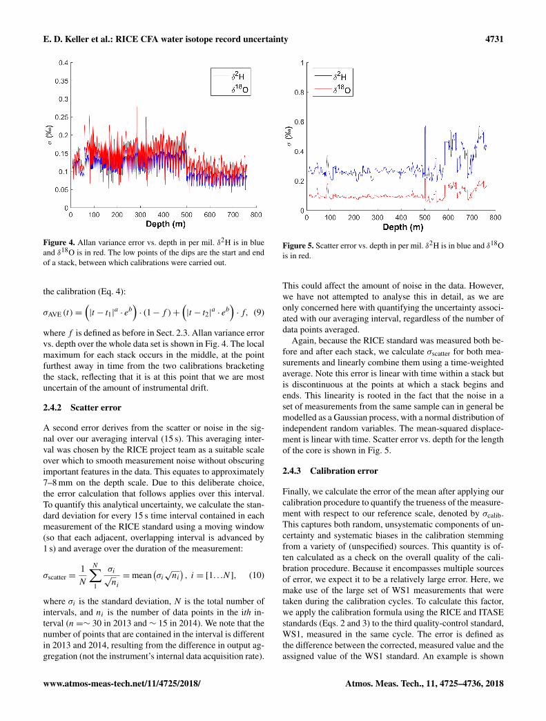
2.4.2 Scatter error

A second error derives from the scatter or noise in the sig-nal over our averaging interval (15 s). This averaging inter-val was chosen by the RICE project team as a suitable scaleover which to smooth measurement noise without obscuringimportant features in the data. This equates to approximately7–8 mm on the depth scale. Due to this deliberate choice,the error calculation that follows applies over this interval.To quantify this analytical uncertainty, we calculate the stan-dard deviation for every 15 s time interval contained in eachmeasurement of the RICE standard using a moving window(so that each adjacent, overlapping interval is advanced by1 s) and average over the duration of the measurement:

σscatter =1N

N∑1

σi√ni=mean

(σi√ni), i = [1. . .N ], (10)

where σi is the standard deviation, N is the total number ofintervals, and ni is the number of data points in the ith in-terval (n=∼ 30 in 2013 and ∼ 15 in 2014). We note that thenumber of points that are contained in the interval is differentin 2013 and 2014, resulting from the difference in output ag-gregation (not the instrument’s internal data acquisition rate).

Figure 5. Scatter error vs. depth in per mil. δ2H is in blue and δ18Ois in red.

This could affect the amount of noise in the data. However,we have not attempted to analyse this in detail, as we areonly concerned here with quantifying the uncertainty associ-ated with our averaging interval, regardless of the number ofdata points averaged.

Again, because the RICE standard was measured both be-fore and after each stack, we calculate σscatter for both mea-surements and linearly combine them using a time-weightedaverage. Note this error is linear with time within a stack butis discontinuous at the points at which a stack begins andends. This linearity is rooted in the fact that the noise in aset of measurements from the same sample can in general bemodelled as a Gaussian process, with a normal distribution ofindependent random variables. The mean-squared displace-ment is linear with time. Scatter error vs. depth for the lengthof the core is shown in Fig. 5.

2.4.3 Calibration error

Finally, we calculate the error of the mean after applying ourcalibration procedure to quantify the trueness of the measure-ment with respect to our reference scale, denoted by σcalib.This captures both random, unsystematic components of un-certainty and systematic biases in the calibration stemmingfrom a variety of (unspecified) sources. This quantity is of-ten calculated as a check on the overall quality of the cali-bration procedure. Because it encompasses multiple sourcesof error, we expect it to be a relatively large error. Here, wemake use of the large set of WS1 measurements that weretaken during the calibration cycles. To calculate this factor,we apply the calibration formula using the RICE and ITASEstandards (Eqs. 2 and 3) to the third quality-control standard,WS1, measured in the same cycle. The error is defined asthe difference between the corrected, measured value and theassigned value of the WS1 standard. An example is shown

www.atmos-meas-tech.net/11/4725/2018/ Atmos. Meas. Tech., 11, 4725–4736, 2018

4732 E. D. Keller et al.: RICE CFA water isotope record uncertainty

Figure 6. Representative δ18O calibration of ice core stack andWS1, using RICE and ITASE standards from the same cycle, 15 smoving average vs. time (measured on 2 July 2014). The differencebetween the true value of WS1 (blue) and the calibrated measuredvalue of WS1 (red) is the calibration error. The error that was ap-plied to the CFA data set is the average difference of all WS1 cali-bration measurements during the melting campaign.

in Fig. 6. We calculated this difference for all calibration cy-cles containing measurements of all three standards (RICE,ITASE and WS1) of sufficient quality (there were 221 suchcalibration cycles in 2013 and 318 in 2014) and then tookthe mean of the differences. Separate error estimates for the2013 and 2014 melting campaigns were calculated and ap-plied only to the data points from the respective year. Thecalibrated values obtained for all of the WS1 measurementsthroughout both campaigns are shown in Fig. S1 in the Sup-plement.

3 Results and discussion

Total error vs. depth for the whole record is shown in Fig. 7and summarized in Table 2. The mean total errors for alldata points are 0.74 ‰ (δ2H) and 0.21 ‰ (δ18O). Separatedby melting campaign, mean total errors in 2013 are 0.85 ‰(δ2H) and 0.22 ‰ (δ18O) and in 2014 they are 0.44 ‰ (δ2H)and 0.19 ‰ (δ18O). The total error reduces sharply at a depthof 500 m due to the switch between 2013 and 2014 cam-paigns and the greatly reduced calibration error in 2014.However, we observe a larger variability in the error in the2014 data. This is mainly a result of the highly variableamount of noise in the measurements, which is discussed be-low.

The mean Allan errors for all data are 0.12 ‰ for δ2Hand 0.14 ‰ for δ18O. Calculated separately by melting cam-paign, the mean errors are 0.13 ‰ (δ2H) and 0.16 ‰ (δ18O)in 2013 and 0.083 ‰ (δ2H) and 0.11 ‰ (δ18O) in 2014. Asexpected, the Allan error peaks at the points in the middle of

the stack, furthest from a calibration (Fig. 4). It is both abso-lutely and proportionally larger for δ18O, as δ18O is typicallymore affected by drift.

The amount of scatter in the data varies considerably overthe length of the record, particularly in 2014. The mean scat-ter errors over the whole record are 0.29 ‰ (δ2H) and 0.10 ‰(δ18O). Separated by melting campaign, the mean errors are0.26 ‰ (δ2H) and 0.093 ‰ (δ18O) in 2013, and 0.37 ‰ (δ2H)and 0.13 ‰ (δ18O) in 2014. On average, the scatter error islarger in 2014, although during the periods of best instrumen-tal performance, σscatter is lower than at any point in 2013.The instrument performance was highly variable in 2014,much more so than 2013. The standard deviations of σscatterare 0.11 ‰ (δ2H) and 0.045 ‰ (δ18O) in 2014, as opposed to0.026 ‰ (δ2H) and 0.012 ‰ (δ18O) in 2013.

Among the three error factors, the general calibration er-ror is the largest contributor to the total error in 2013: σcalib(δ2H)= 0.80‰ and σcalib (δ

18O)= 0.12‰. However, thiserror is greatly reduced for 2014: σcalib (δ

2H)= 0.22‰ andσcalib (δ

18O)= 0.078‰, reflecting the improved measure-ment of the assigned values of the standards. We were notable to measure the standards against VSMOW-SLAP usingthe 2013 CFA set-up (time constraints did not permit us toconduct additional measurements after the 2013 campaignconcluded, as our instrument was sent to the manufacturerfor modification), which would provide a better comparisonbetween measured and assigned values, following from theprinciple of identical treatment (Werner and Brand, 2001).The 2013 σcalib is thus likely to be a very conservative es-timate of the error. In addition, the assigned value of WS1is well outside the range of the RICE ice core and is muchgreater than the RICE and ITASE standards, and thus RICEand ITASE could be considered poor choices for calibrat-ing WS1. The two calibration standards, RICE and ITASE,were chosen to be similar in isotopic value to the ice coresamples being measured (Werner and Brand, 2001), with thequality-control standard being of secondary concern. Ideally,we would use a quality-control standard that falls within therange of the values of our two calibration standards. Whilewe could have used WS1 and ITASE as our calibration stan-dards and RICE as a quality-control, WS1 is less appropriatethan RICE for calibrating the range of isotopic values foundin the ice core. Testing the sensitivity of the calibration er-ror to our selection of quality-control standards, however, isoutside the scope of this paper.

The scatter error dominates the total error in 2014. Themagnitude of this error was highly variable from day to day,and thus the total error also varied considerably. There weresome periods in which the instrument performed exception-ally well. During these periods, total errors were as low as0.3 ‰ (δ2H) and 0.1 ‰ (δ18O). These represent the high endof system capability. However, for much of the 2014 melt-ing campaign the total errors were closer to the average of0.44 ‰ (δ2H) and 0.19 ‰ (δ18O).

Atmos. Meas. Tech., 11, 4725–4736, 2018 www.atmos-meas-tech.net/11/4725/2018/

E. D. Keller et al.: RICE CFA water isotope record uncertainty 4733

Table 2. Summary of uncertainty estimates in per mil (‰).

δ18O (‰) δ2H (‰)

Error factor 2013 2014 Combined 2013 2014 Combined

Allan ±0.16 ±0.11 ±0.14 ±0.13 ±0.083 ±0.12Scatter ±0.093 ±0.13 ±0.10 ±0.26 ±0.37 ±0.29Calibration ±0.12 ±0.078 n/a∗ ±0.80 ±0.22 n/aTotal ±0.22 ±0.19 ±0.21 ±0.85 ±0.43 ±0.76

∗ n/a stands for “not applicable”.

Figure 7. Total uncertainty vs. depth, along with each individual error factor in per mil. (a): δ2H. (b): δ18O. There is a noticeable discontinuityat 500 m; the melting campaign was paused at 500 m in 2013, and melting was resumed in 2014 with a modified set-up. The reducedcalibration error in 2014 is responsible for the large step down in total error.

There are three main possible reasons for the large varia-tions in performance in 2014. They are (1) response to breaksin the ice and associated bubbles; (2) performance degra-dation due to unexpected levels of drill fluid in the meltstream (a mixture of Estisol-240 and Coasol was used tokeep the drill hole open; although all pieces of ice were thor-oughly cleaned before melting, some contamination occurredthrough existing microfractures in the ice); and (3) leaksor valve degradation in the laser spectrometer, which oper-ates under vacuum. There were significantly more perfor-mance issues in 2014. In addition to the different set-up andgradual build-up of drill fluid in the instruments over time,the ice itself was of poorer quality at lower depths (espe-cially in the brittle ice zone at depths below 500 m; Pyne

et al., 2018), containing more breaks that caused interrup-tions in the CFA measurements and possible drill fluid con-tamination. Although we have only anecdotal evidence, themore frequent stopping and restarting of the system in 2014seemed to introduce more noise into the measurements.

Because the campaign was conducted to operate manymeasurement systems simultaneously, as is characteristic ofice core CFA campaigns, it was typically not possible to con-duct comprehensive performance tests and systematic evalu-ations during the 1 day of downtime in each week-long, 7-day cycle. As a result, the precise sources of performancedeterioration were difficult to isolate. Our method for calcu-lating uncertainty is designed to capture the changing day-to-day conditions resulting from a range of system variations

www.atmos-meas-tech.net/11/4725/2018/ Atmos. Meas. Tech., 11, 4725–4736, 2018

4734 E. D. Keller et al.: RICE CFA water isotope record uncertainty

and performance issues, even if it is not possible to pinpointthe exact cause.

4 Summary and conclusions

We have described a systematic approach to the data process-ing and calibration for the RICE CFA stable water isotopedata set and presented a novel methodology to calculate un-certainty estimates for each data point derived from three fac-tors: Allan deviation, scatter, and calibration accuracy. Themean total errors for all data points are 0.74 ‰ (δ2H) and0.21 ‰ (δ18O). Mean total errors in 2013 are 0.85 ‰ (δ2H)and 0.22 ‰ (δ18O) and in 2014 they are 0.44 ‰ (δ2H) and0.19 ‰ (δ18O). This represents a significant achievement inthe precision of high-resolution CFA water isotope measure-ments, and documentation of uncertainty calculations for iso-tope analyses in a continuous measurement campaign com-prising multiple complex measurement systems.

The isotope analyser system performed exceptionally wellduring some time intervals in 2014, demonstrating high ca-pability, even though this was not sustained. The variabilityin quality could be due to poor ice quality, interruptions in theCFA measurements, the build-up of residual drill fluid in theinstrument, and/or leaks and valve degradation. Most likely,it was a combination of all of these factors.

The more accurate measurement of our laboratory wa-ter standards for the 2014 melting campaign enabled us toreduce the uncertainty considerably for the data at depthsgreater than 500 m. More generally, a reduction in the uncer-tainty in the system could be achieved through more rapidcalibration cycles, enabling both the insertion of calibra-tion during stacks and more rapid troubleshooting to isolatecauses of degraded performance.

Our uncertainty estimates do not take into account the ad-ditional uncertainty introduced from the smoothing of thedata during the melting procedure and the measurement re-sponse time. This is an important issue, particularly for deep,older ice, where annual layers are greatly compressed andmeasurement resolution is crucial to the ability to date thecore accurately. The degree of mixing in the melting pro-cedure itself can be controlled through the melting rate andthe diameter of tubing leading from the melter to the CFAinstruments. Our system was designed primarily for highthroughput and multiple, simultaneous measurements. How-ever, these parameters can be adjusted to increase resolutionfor older ice (the very bottom of the RICE core has yet to bemeasured).

The volume of the evaporation chamber is usually a lim-iting factor in the temporal resolution and response time ofthe IWA and can introduce a significant amount of uncer-tainty. While we reduced the volume of the chamber fromthe manufacturer’s default of 1.1 L to 40 mL (Emanuelssonet al., 2015), there is still a finite amount of time required tofill and replace the chamber with new sample. We estimate

that our depth resolution was between 1.0 and 3.0 cm (Pyneet al., 2018). A more comprehensive evaluation of the effectof the mixing inherent in the melting and measurement pro-cedure on the overall uncertainty is beyond the scope of thispaper but is an important consideration for future work.

Data availability. The RICE CFA stable isotope data are currentlyembargoed but will be made available in a forthcoming publica-tion. Data for the past 2700 years are available as a supplement toBertler et al. (2018) (https://doi.org/10.15.94/PANGAEA.880396)and at http://www.rice.aq/data-collection.html (last access: 8 Au-gust 2018).

Supplement. The supplement related to this article is availableonline at: https://doi.org/10.5194/amt-11-4725-2018-supplement.

Author contributions. EK and TB designed and calculated the CFAstable isotope uncertainty estimates. NB, TB and DE designed theCFA set-up and took the measurements. EK and SC processed theCFA data. AP took the laboratory water standard measurements. Allauthors contributed to the writing of this paper.

Competing interests. The authors declare that they have no conflictof interest.

Acknowledgements. Funding for this project was provided by theNew Zealand Ministry of Business, Innovation, and Employmentgrants through Victoria University of Wellington (RDF-VUW-1103, 15-VUW-131), GNS Science (540GCT32, 540GCT12), andAntarctica New Zealand (K049). We are indebted to everyone fromthe 2013 and 2014 RICE core processing teams. We would like tothank the Mechanical and Electronic Workshops of GNS Sciencefor technical support during the RICE core progressing campaigns.This work is a contribution to the Roosevelt Island ClimateEvolution (RICE) programme, funded by national contributionsfrom New Zealand, Australia, Denmark, Germany, Italy, China,Sweden, UK and USA. The main logistic support was provided byAntarctica New Zealand and the US Antarctic Program.

Edited by: Frank KepplerReviewed by: three anonymous referees

References

Aemisegger, F., Sturm, P., Graf, P., Sodemann, H., Pfahl, S., Knohl,A., and Wernli, H.: Measuring variations of δ18O and δ2H in at-mospheric water vapour using two commercial laser-based spec-trometers: an instrument characterisation study, Atmos. Meas.Tech., 5, 1491–1511, https://doi.org/10.5194/amt-5-1491-2012,2012.

Allan, D. W.: Statistics of atomic frequency standards in the near-infrared, Proc. IEEE, 54, 221–231, 1966.

Atmos. Meas. Tech., 11, 4725–4736, 2018 www.atmos-meas-tech.net/11/4725/2018/

E. D. Keller et al.: RICE CFA water isotope record uncertainty 4735

Analytical Methods Committee: Technical Brief, No. 13, Terminol-ogy – the key to understanding analytical science, Part 1: Accu-racy, precision and uncertainty, Roy. Soc. Ch., September 2003.

Baer, D. S., Paul, J. B., Gupta, M., and O’Keefe, A.: Sensitive ab-sorption measurements in the near-infrared region using off-axisintegrated-cavity-output spectroscopy, Appl. Phys. B-Lasers O,75, 261–265, 2002.

Bertler, N. A. N., Conway, H., Dahl-Jensen, D., Emanuelsson, D.B., Winstrup, M., Vallelonga, P. T., Lee, J. E., Brook, E. J., Sev-eringhaus, J. P., Fudge, T. J., Keller, E. D., Baisden, W. T., Hind-marsh, R. C. A., Neff, P. D., Blunier, T., Edwards, R., Mayewski,P. A., Kipfstuhl, S., Buizert, C., Canessa, S., Dadic, R., Kjær,H. A., Kurbatov, A., Zhang, D., Waddington, E. D., Baccolo,G., Beers, T., Brightley, H. J., Carter, L., Clemens-Sewall, D.,Ciobanu, V. G., Delmonte, B., Eling, L., Ellis, A., Ganesh, S.,Golledge, N. R., Haines, S., Handley, M., Hawley, R. L., Hogan,C. M., Johnson, K. M., Korotkikh, E., Lowry, D. P., Mandeno,D., McKay, R. M., Menking, J. A., Naish, T. R., Noerling, C.,Ollive, A., Orsi, A., Proemse, B. C., Pyne, A. R., Pyne, R. L.,Renwick, J., Scherer, R. P., Semper, S., Simonsen, M., Sneed, S.B., Steig, E. J., Tuohy, A., Venugopal, A. U., Valero-Delgado, F.,Venkatesh, J., Wang, F., Wang, S., Winski, D. A., Winton, V. H.L., Whiteford, A., Xiao, C., Yang, J., and Zhang, X.: RooseveltIsland Climate Evolution (RICE) ice core isotope record data set,available at: https://doi.org/10.1594/PANGAEA.880396 (last ac-cess: 4 August 2018), 2017.

Bertler, N. A. N., Conway, H., Dahl-Jensen, D., Emanuelsson, D.B., Winstrup, M., Vallelonga, P. T., Lee, J. E., Brook, E. J., Sev-eringhaus, J. P., Fudge, T. J., Keller, E. D., Baisden, W. T., Hind-marsh, R. C. A., Neff, P. D., Blunier, T., Edwards, R., Mayewski,P. A., Kipfstuhl, S., Buizert, C., Canessa, S., Dadic, R., Kjær,H. A., Kurbatov, A., Zhang, D., Waddington, E. D., Baccolo,G., Beers, T., Brightley, H. J., Carter, L., Clemens-Sewall, D.,Ciobanu, V. G., Delmonte, B., Eling, L., Ellis, A., Ganesh, S.,Golledge, N. R., Haines, S., Handley, M., Hawley, R. L., Hogan,C. M., Johnson, K. M., Korotkikh, E., Lowry, D. P., Mandeno,D., McKay, R. M., Menking, J. A., Naish, T. R., Noerling, C.,Ollive, A., Orsi, A., Proemse, B. C., Pyne, A. R., Pyne, R. L.,Renwick, J., Scherer, R. P., Semper, S., Simonsen, M., Sneed, S.B., Steig, E. J., Tuohy, A., Venugopal, A. U., Valero-Delgado,F., Venkatesh, J., Wang, F., Wang, S., Winski, D. A., Winton,V. H. L., Whiteford, A., Xiao, C., Yang, J., and Zhang, X.: TheRoss Sea Dipole – temperature, snow accumulation and sea icevariability in the Ross Sea region, Antarctica, over the past 2700years, Clim. Past, 14, 193–214, https://doi.org/10.5194/cp-14-193-2018, 2018.

Bigler, M., Svensson, A., Kettner, E., Vallelonga, P., Nielsen, M. E.,and Steffensen, J. P.: Optimization of high-resolution continuousflow analysis for transient climate signals in ice cores, Environ.Sci. Technol., 45, 4483–4489, 2011.

Carter, J. F. and Fry, B.: Ensuring the reliability of stable isotoperatio data – beyond the principle of identical treatment, Anal.Bioanal. Chem., 405, 2799–2814, 2013.

Coplen, T. B.: Guidelines and Recommended Terms for Expressionof Stable- Isotope-Ratio and Gas-Ratio Measurement Results,Rapid Commun. Mass Spectrom., 25, 2538–2560, 2011.

Dansgaard, W.: Stable isotopes in precipitation, Tellus, 16, 436–468, https://doi.org/10.1111/j.2153-3490.1964.tb00181.x, 1964.

Emanuelsson, B. D., Baisden, W. T., Bertler, N. A. N., Keller,E. D., and Gkinis, V.: High-resolution continuous-flow analy-sis setup for water isotopic measurement from ice cores us-ing laser spectroscopy, Atmos. Meas. Tech., 8, 2869–2883,https://doi.org/10.5194/amt-8-2869-2015, 2015.

Emanuelsson, B. D., Bertler, N. A. N., Neff, P. D., Renwick, J. A.,Markle, B. R., Baisden, W. T., and Keller, E. D.: The role ofAmundsen–Bellingshausen Sea anticyclonic circulation in forc-ing marine air intrusions into West Antarctica, Clim. Dyn., 1–18,2018.

Epstein, S., Sharp, R. P., and Goddard, I.: Oxygen-isotope ratios inAntarctic snow, firn, and ice, J. Geol., 71, 698–720, 1963.

Gkinis, V., Popp, T. J., Blunier, T., Bigler, M., Schüpbach, S., Ket-tner, E., and Johnsen, S. J.: Water isotopic ratios from a contin-uously melted ice core sample, Atmos. Meas. Tech., 4, 2531–2542, https://doi.org/10.5194/amt-4-2531-2011, 2011.

Gonfiantini, R.: Standards for stable isotope measurements in natu-ral compounds, Nature, 271, 534–536, 1978.

Jones, T. R., White, J. W. C., Steig, E. J., Vaughn, B. H., Mor-ris, V., Gkinis, V., Markle, B. R., and Schoenemann, S. W.:Improved methodologies for continuous-flow analysis of stablewater isotopes in ice cores, Atmos. Meas. Tech., 10, 617–632,https://doi.org/10.5194/amt-10-617-2017, 2017.

Kaufmann, P. R., Federer, U., Hutterli, M. A., Bigler, M., Schüp-bach, S., Ruth, U., Schmitt, J., and Stocker, T. F.: An ImprovedContinuous Flow Analysis System for High-Resolution FieldMeasurements on Ice Cores, Environ. Sci. Technol., 42, 8044–8050, https://doi.org/10.1021/es8007722, 2008.

Kirchner, J.: Data Analysis Toolkits: available at: http://seismo.berkeley.edu/~kirchner/eps_120/Toolkits/Toolkit_05.pdf (lastaccess: 31 May 2018), 2001.

Kurita, N., Newman, B. D., Araguas-Araguas, L. J., and Aggarwal,P.: Evaluation of continuous water vapor δD and δ18O measure-ments by off-axis integrated cavity output spectroscopy, Atmos.Meas. Tech., 5, 2069–2080, https://doi.org/10.5194/amt-5-2069-2012, 2012.

Küttel, M., Steig, E. J., Ding, Q., Monaghan, A. J., and Battisti,D. S.: Seasonal climate information preserved in West Antarcticice core water isotopes: relationships to temperature, large-scalecirculation, and sea ice, Clim. Dyn., 39, 1841–1857, 2012.

Lee, J. E., Brook, E. J., Bertler, N. A. N., Buizert, C., Baisden, T.,Blunier, T., Ciobanu, V. G., Conway, H., Dahl-Jensen, D., Fudge,T. J., Hindmarsh, R., Keller, E. D., Parrenin, F., Severinghaus,J. P., Vallelonga, P., Waddington, E. D., and Winstrup, M.: An83 000 year old ice core from Roosevelt Island, Ross Sea, Antarc-tica, Clim. Past Discuss., https://doi.org/10.5194/cp-2018-68, inreview, 2018.

Meier-Augenstein, W.: Stable isotope forensics: an introduction tothe forensic application of stable isotope analysis, Vol. 3, JohnWiley & Sons, Dundee, UK, 2017.

NGRIP Members: High-resolution record of Northern Hemisphereclimate extending into the last interglacial period, Nature, 431,147–151, 2004.

Paul, D., Skrzypek, G., and Fórizs, I.: Normalization of mea-sured stable isotopic compositions to isotope reference scales– a review, Rapid Commun. Mass Spectrom., 21, 3006–3014,https://doi.org/10.1002/rcm.3185, 2007.

Pyne, R. L., Keller, E. D., Canessa, S., Bertler, N. A. N., Pyne, A. R.,Mandeno, D., Vallelonga, P., Semper, S., Kjær, H. A., Hutchin-

www.atmos-meas-tech.net/11/4725/2018/ Atmos. Meas. Tech., 11, 4725–4736, 2018

4736 E. D. Keller et al.: RICE CFA water isotope record uncertainty

son, E., and Baisden, W. T.: A Novel Approach to Process BrittleIce for Water Isotope Continuous Flow Analysis, J. Glaciol., 64,289–299, https://doi.org/10.1017/jog.2018.19, 2018.

Sinclair, K. E., Bertler, N. A. N., Trompetter, W. J., and Baisden, W.T.: Seasonality of airmass pathways to coastal Antarctica: rami-fications for interpreting high-resolution ice core records, J. Cli-mate, 26, 2065–2076, 2013.

Steig, E. J., Ding, Q., White, J. W. C., Kuttel, M., Rupper, S. B.,Neumann, T. A., Neff, P. D., Gallant, A. J., Mayewski, P. A.,Taylor, K. C., and Hoffmann, G.: Recent climate and ice-sheetchanges in West Antarctica compared with the past 2000 years,Nat. Geosci., 6, 372–375, https://doi.org/10.1038/ngeo1778,2013.

Sturm, P. and Knohl, A.: Water vapor δ2H and δ18O measure-ments using off-axis integrated cavity output spectroscopy, At-mos. Meas. Tech., 3, 67–77, https://doi.org/10.5194/amt-3-67-2010, 2010.

Vinther, B. M., Clausen, H. B., Johnsen, S. J., Rasmussen, S.O., Andersen, K. K., Buchardt, S. L., Dahl-Jensen, D., Seier-stad, I. K., Siggaard-Andersen, M. L., Steffensen, J. P., andSvensson, A.: A synchronized dating of three Greenland icecores throughout the Holocene, J. Geophys. Res., 111, D13102,https://doi.org/10.1029/2005JD006921, 2006.

Werle, P.: Accuracy and precision of laser spectrometers for tracegas sensing in the presence of optical fringes and atmosphericturbulence, Appl. Phys. B-Lasers O., 102, 313–329, 2011.

Werner, R. A. and Brand, W. A.: Referencing strategies and tech-niques in stable isotope ratio analysis, Rapid Commun. MassSpectrom., 15, 501–519, 2001.

Winstrup, M., Vallelonga, P., Kjær, H. A., Fudge, T. J., Lee, J.E., Riis, M. H., Edwards, R., Bertler, N. A. N., Blunier, T.,Brook, E. J., Buizert, C., Ciobanu, G., Conway, H., Dahl-Jensen,D., Ellis, A., Emanuelsson, B. D., Keller, E. D., Kurbatov, A.,Mayewski, P., Neff, P. D., Pyne, R., Simonsen, M. F., Svens-son, A., Tuohy, A., Waddington, E., and Wheatley, S.: A 2700-year annual timescale and accumulation history for an ice corefrom Roosevelt Island, West Antarctica, Clim. Past Discuss.,https://doi.org/10.5194/cp-2017-101, in review, 2017.

Atmos. Meas. Tech., 11, 4725–4736, 2018 www.atmos-meas-tech.net/11/4725/2018/