Research Papers in Economics No. 5/16

Calibrating the Equilibrium Condition of a New Keynesian Model with Uncertainty Tobias Kranz

Calibrating the Equilibrium Condition of a

New Keynesian Model with Uncertainty*

Tobias Kranz†

University of Trier, Germany

May 18, 2017

Abstract

This paper presents a theoretical analysis of the simulated impact of un-

certainty in a New Keynesian model. In order to incorporate uncertainty, the

basic three-equation framework is modified by higher-order approximation

resulting in a non-linear (dynamic) IS curve. Using impulse response anal-

yses to examine the behavior of the model after a cost shock, I find interest

rates in the version with uncertainty to be lower in contrast to the case under

certainty.

JEL Codes: E12, E17, E43, E47, E52.

Keywords: Impulse Response, New Keynesian Model, Persistent Stochas-

tic Shocks, Quadratic Approximation, Simulation, Uncertainty.

*Thanks to Matthias Neuenkirch for his helpful comments on earlier versions of the paper.I also thank participants of the 11th Workshop for Macroeconomics and Business Cycles at ifoDresden, particularly Stefan Homburg and Christian Scharrer, for helpful comments. The usualdisclaimer applies.

†Email: s4tokran@uni-trier.de.

1

1 Introduction

For the last 20 years, the New Keynesian framework has been one of the work-

horses of macroeconomic analysis. The framework combines market frictions

with optimization behavior by the model’s agents, and, in its original construc-

tion, assumes perfect foresight. However, the treatment of uncertainty is an im-

portant issue since its effect can fundamentally change the prediction of these

models.

This paper examines possible effects of uncertainty in a simple New Keyne-

sian model (NKM) augmented with stochastic terms and non-linearity that enters

the model through a second-order Taylor approximation regarding the IS curve.

In line with the literature (see, among others, the textbooks by Galı 2015 and

Walsh 2010), cost shock and demand shock are utilized for the New Keynesian

Phillips curve (NKPC) and the forward-looking IS curve, respectively. Schmitt-

Grohe and Uribe (2004) use second-order approximation in neoclassical growth

models. Bauer and Neuenkirch (2015) were the first to use such a framework

in the context of a NKM and found empirical evidence that central banks, in-

deed, take the resulting uncertainty into account. Moreover, their paper pro-

vides strong arguments that linear macroeconomic models found in monetary

policy literature are less than optimal (see also Boneva et al. 2016 and Fernandez-

Villaverde et al. 2011). The main contribution this paper offers is the analysis of

how the economy evolves after cost shocks, and the extent to which persistence

plays a role.

In order to extend the NKM, we include a quadratic approximation in all de-

rived equations. First, in the analytical part, demand and supply side (includ-

ing monopolistic competition and price rigidity), where firms use second-order

approximation when setting the prices, yields the NKPC. Second, the forward-

looking IS curve with uncertainty follows from the households’ Euler equation.

This method differs fundamentally from standard approaches. Finally, to close

the model, a (standard) targeting rule is derived by the central bank’s optimiza-

tion under discretion.

After adding AR(1) processes to the derived equations, conditional expec-

tations and variances can be substituted by solving forward. Next, parameter

values are selected for the resulting equilibrium condition (or instrument rule)

with the focus on persistence and shock strength. A numerical simulation anal-

2

yzes differences to the basic model. Finally, to examine the adjustment of macro

variables in the medium term, impulse responses are carried out and contrasted

with the linear counterpart.1 In the same vein, but without an explicit derivation

of the uncertainty, De Paoli and Zabczyk (2013) compare linear and non-linear

models.

The remainder of this paper is organized as follows. Section 2 derives a basic

version of the NKM augmented with a quadratic IS curve. Section 3 expands this

model with shocks and discusses the resulting equilibrium condition. Section 4

carries out the numerical simulation of both the static equilibrium condition and

the dynamic view of an impulse response analysis. Section 5 concludes.

2 New Keynesian Model with Uncertainty

2.1 New Keynesian Phillips Curve

For deriving the NKPC, two optimization problems involving private households

and firms are employed, leading to aggregated demand and supply. Furthermore,

price rigidity is modeled using the method introduced by Calvo (1983).2 From

the Calvo Pricing section on, the time index t is used because it is needed to make

a distinction between the different periods.

Demand and Supply Side

Consumers

On the demand side, the representative consumer can choose from a variety of

goods Cξ which results in an aggregate consumption of C. Usually, the CES func-

tion is used to model monopolistic competition,3 one of the two market frictions

incorporated into the NKPC:

C =(∫ 1

0C

ε−1εξ dξ

) εε−1

. (1)

1To keep the framework easily understandable, government, investments, money supply, andlabor markets are omitted. Consequently, neither money holdings nor working hours (or leisuretime) will enter the households’ utility function.

2This paper focuses on the standard approach. For non-linear versions of the Phillips curvesee the articles by Collard and Juillard (2001), Dolado et al. (2005), and Schaling (2004).

3Dixit and Stiglitz (1977) developed this approach. Although they used a discrete sum andno integral, they received the same results.

3

Here, ξ ∈ [0,1] can be viewed as a continuum of firms from 0 to 100%. The

exponent is a measure for the substitutability between the goods Cξ , where ε

represents the elasticity of substitution.

A Hicksian-like optimization helps to solve for the demand curve by means

of the Lagrangian function:

L (Cξ ,λ) =∫ 1

0Pξ ·Cξ dξ −λ

(∫ 1

0C

ε−1εξ dξ

) εε−1

−C

. (2)

Since firms have pricing power, the representative consumer takes prices Pξas given. Minimizing expenditures

∫PξCξ with the constraint of a certain con-

sumption level C requires the following first-order conditions:4

∂L∂Cτ

= Pτ −λC− 1ε

τ

(∫ 1

0C

ε−1εξ dξ

) 1ε−1

= 0. (3)

Differentiating with respect to λ provides the constraint, Eq.(1). Rearranging

condition (3) and defining λ ≡ P as the aggregated price level yields

Cτ =(PPτ

)εC, (4)

the demand for good i.5 The aggregated price level can be described by substi-

tuting this in Eq.(1). Rearranging the formula gives us:

P =(∫ 1

0P 1−εξ dξ

) 11−ε

. (5)

The lack of investment and governmental spendings in this model leads to

Yτ = Cτ . Each firms’ production Yτ will be consumed completely by private

households and hence Y = C.

Firms

Because any single firm is too small to directly influence other prices or produc-

tions, each firm takes the aggregated demand function and the aggregated price4Note that τ denotes a continuum of derivatives.5When the consumption constraint is relaxed by one unit, total consumption expenditures

(see Galı 2015, 53) will increase to (C+1)P = CP +P , where P is the amount by which the optimumwill change. This is exactly the information the Lagrange multiplier λ contains. See AppendixA.1 for the missing steps in this paragraph.

4

level P as given. It chooses its own price Pτ and faces the typical (real) profit

maximization problem

maxPτ ,Yτ

{PτYτP−K(Yτ )

}(6)

with the cost function K(.). Using Eq.(4), the first-order condition is straightfor-

ward and leads to

P ∗τ =( εε − 1

)K ′(Yτ ) · P , (7)

an important result that states that the optimal price P ∗τ equals the nominal

marginal costs and a mark-up bigger than one for all ε > 1.6 Log-linearizing and

using the fact that the long-run marginal costs equal the multiplicative inverse

of the firms’ mark-up (Kss = 1− ε−1) yields

p∗τ − p = ψyτ , (8)

where ψ is a parameter for the long-run cost elasticity and, therefore, log de-

viations of marginal costs from their long-run trend are assumed to be linear.7

Inserting the log-version of Eq.(4) gives

p∗τ − p =(

ψ

1 +ψε

)y. (9)

Making use of y, the GDP growth rate around the steady state, as an approxi-

mation for y and using αψ ∈ [0,1[ as a summarizing parameter, Eq.(9) yields

p∗τ − p = αψy, (10)

a description of the steady state output growth rate, depending on price level

growth and microeconomic behavior. The next section introduces a non-optimal

price setting scheme which replicates the actual observed economic patterns.8

Calvo Pricing

Nominal rigidities, the second market friction in the basic NKM, are imple-

mented through the assumption that the firms’ infrequent price adjustment fol-6See Appendix A.2 for the missing steps.7Note that lower case letters denote the log value of a variable in capital letters minus their

long-run log value, e.g. y = ln(Y )− ln(Yss). See Appendix A.3 for the missing steps.8See the survey by Taylor (1999), that came to abundant evidence. See also Galı (2015, 7–8)

for a literature overview.

5

lows an exogenous Poisson process.9 This implies that all firms have a constant

probability (φ) of being unable to update their price in each period withφ ∈ [0,1[

(i.e., φ = 0 in the absence of price rigidity). It is crucial that price setters do not

know how long the nominal price will remain in place. Only the expected value

is known due to probabilities that are all equal and constant for all firms and pe-

riods. This implies a probability of φj for having today’s same price in j periods,

so the average expected duration between price changes will be 1/(1−φ).

From this point forward, the time index t will be used because more than

one period is being considered. Simultaneously, the firm index τ is no longer

important since it is sufficient to calculate with a share of firms φ (or 1 − φ).

Hence, p∗τ ≡ p∗t and p ≡ pt. When xt is the price that firms set in period t (provided

they are able to do so), the following applies:

xt =pt −φpt−1

1−φ⇒ Etxt+1 =

Etpt+1 −φpt1−φ

. (11)

Because firms act on the probability of not being able to adjust prices in future

periods, they attempt to establish a price xt that is not necessarily the optimal

price p∗t , derived in the previous section. Also, in the presence of price rigidities,

xt , p∗t generally holds.

To reveal the mechanics behind the staggered price setting, it is convenient

to verbally treat pt and xt as level variables. Strictly speaking, firms set price

growth paths in the following optimization problem rather than maximizing a

discounted profit as the difference between revenue and costs.10 In the follow-

ing, the optimal reset price, determined by the discounted sum of future profits,

is derived through a quadratic approximation of the per-period deviation from

maximum-possible profit with β ∈ [0,1[, the discount factor over an infinite plan-

ning horizon. Therefore, firms minimize their loss function, the discounted de-

viations from p∗t over all t:

minxt

Etk ∞∑

j=0

βjφj(xt − p∗t+j

)2

. (12)

9Calvo (1983) originally wrote his article in continuous time. However, using discrete periodsimmensely helps the clearness and is more realistic with regard to how firms actually operate.Moreover, Calvo (1983, 396–397) shows the equivalence of both approaches.

10See Walsh (2010, 241–242) for the use of level variables in Calvo pricing.

6

The parameter k > 0 enters the loss function multiplicatively and indicates all

exogenous factors that will influence the costs of not setting the optimal price in

each period.11 The first-order condition is

∂∂xt

= Et

2k ∞∑j=0

(βφ)j(xt − p∗t+j)

= 0. (13)

After rearranging12 and expressing x through p with Eq.(11), it follows that

pt −φpt−1 = βφ(Etpt+1 −φpt) + (1−φ)(1− βφ)p∗t (14)

only contains parameters and variants of the variable p. Expressing p through

π,13 as well as isolating (p∗t − pt) and replacing it with the result in Eq.(10), gives

πt = βEtπt+1 +αψ(1−φ)(1− βφ)

φyt. (15)

In a final step, a summarizing parameter κ > 0 for all parameters, multiplied

with yt, will be defined. This yields the NKPC:14

πt = βEtπt+1 +κyt. (16)

Both the expected inflation rate Etπt+1 and the GDP growth rate around the

steady state yt (or output gap) have a positive impact on πt since β,κ > 0. More-

over, the slope of the NKPC (κ), depends on all four parameters (β,ψ,ε, and φ)

of this section.15

11Note that it can also come up as an additive term or any other positive monotonic transfor-mation and does not alter the results.

12See Appendix A.4 for the missing steps.13

pt − pt−1 = lnPt − lnPss − (lnPt−1 − lnPss) = ln(PtPt−1

)= ln(1 +πt) ≈ πt .

14In contrast to the IS curve discussed in the next section, the NKPC is still linear. Simulationsin Matlab show that the effect of a non-linear NKPC is rather small. That is why our focus onuncertainty relies on the IS curve.

15Depending on the exact model, the slope of the NKPC can have a slightly different meaning,e.g. Walsh (2010, 336) uses a measure for the firm’s real marginal costs instead of the output gap.

7

2.2 The Quadratic IS Curve

The objective is to derive an Euler equation via maximizing utility with a dynamic

budget constraint. Initially, it is not necessary to formulate an explicit utility

function. On the contrary, the general marginal utility provides a better insight

into the intertemporal mechanics. The only specific assumption is not taking

money, working hours or any other possible utility-gainer into consideration. The

utility function solely relies on consumption, thus, households maximize their

intertemporal discounted utility

maxCt

Et ∞∑s=t

βs−tU (Cs)

. (17)

Taking into account an intertemporal budget constraint with prices and the

interest rate it, the maximization problem leads16 to the Euler equation

U ′(Ct) = β(1 + it) ·Et[Pt ·U ′(Ct+1)

Pt+1

], (18)

revealing the intertemporal relationship of the marginal utility out of consump-

tion. Marginal utility in period t equals the counterpart in t + 1, corrected by

discount factor, nominal interest rate, and the ratio of current and expected fu-

ture price level. Assuming it rises, marginal utility in t would also rise relative

to period t + 1. Given the diminishing marginal utility property and, therefore,

concavity, consumption will be higher in the future.17

One convenient formulation for such a function is U (Ct) = (1 − σ )−1 · (C1−σt −

1) with σ > 0 implying 1/σ as the intertemporal elasticity of substitution (IES).

Substituting this in the Euler equation gives

Y −σt = β(1 + it) ·Et[Pt ·Y −σt+1

Pt+1

], (19)

when recalling the market clearing condition Y = C. The long-run real interest

rate r enters the equation through β since it equals 1/β − 1.18

16See Appendix A.5 for the missing steps.17Note that present consumption could also increase because of the income effect.18The relation follows from the steady state Euler equation. See Galı (2015, 132) for a more

complex definition of the long-term real interest rate.

8

Quadratic Approximation

Eq.(19) can be prepared for quadratic approximation by inserting 1/(1 + r) for

β, treating t-measurable variables as constants for the conditional expectation,

rearranging, and taking logs:

ln(

1 + r1 + it

)= lnEt

[(Yt+1

Yt

)−σ ]− lnEt

[Pt+1

Pt

]. (20)

Ignoring Jensen’s inequality is equivalent to first-order Taylor series expan-

sions of both logarithm and exponential function. Furthermore, the right side of

Eq.(20) can be written as19

' Et

[ln

((Yt+1

Yt

)−σ )]−Et

[ln

(Pt+1

Pt

)](21)

and thereby be expressed in growth rates:20

Et[−σ ln(1 + yt+1)]−Et[ln(1 +πt+1)]. (22)

Instead of linearizing, the logarithm will be represented by a second-degree

polynomial:21

≈ Et[−σ

(yt+1 −

12yt+1

2)]−Et

[πt+1 −

12π2t+1

](23.1)

= −σEtyt+1 +σ2Etyt+1

2 −Etπt+1 +12Etπ

2t+1 (23.2)

= σyt − σEtyt+1 +σ2Etyt+1

2 −Etπt+1 +12Etπ

2t+1. (23.3)

Bringing together the linearized form of the left side in Eq.(20) yields the

quadratic IS curve:

yt = Etyt+1 −1σ

(it − r −Etπt+1)− 12σEtπ

2t+1 −

12Etyt+1

2. (24)

Referring to the original graphical IS relation (in the y/i–space), the curve

shifts to the right if the long-term real interest rate r, the output gap expectations

Etyt+1 or the inflation expectations Etπt+1 rise. However, the slope will rise and

19See Appendix A.6 for the missing steps.20Note that the use of the actual GDP growth rate yt+1 in Eq.(22) is merely for clarity. The

relationship between yt+1 and yt+1 is: yt+1 ≈ yt+1 + yt .21See Appendix A.7 for more detail.

9

the curve becomes flatter if the intertemporal elasticity of substitution (1/σ ) rises.

The second-order terms have a negative effect on yt. However, Eq.(24) is not in

reduced form since the last term still contains yt. The formula for the conditional

variance,22 can be utilized to show the second moments’ influence in detail:

yt = Etyt+1 −1σ

(it − r −Etπt+1)− 12σV artπt+1 −

12V artyt+1

− 12σ

(Etπt+1)2 − 12

(Etyt+1)2. (25)

In a first step, looking only at the variances23 and solving for the interest rate

yields

it = −σyt + r +Etπt+1 + σEtyt+1 −12V artπt+1 −

σ2V artyt+1 − . . . , (26)

which states that uncertainty would shift the curve to the left compared to the

original IS curve. Considering the second moment, there are two additional ef-

fects namely expected output gap growth affects the slope and a variation of the

curve’s shape. That is because the last term of Eq.(25) contains yt and yt2:

−12

(Etyt+1 − yt)2 = −12

(Etyt+1)2 +Etyt+1 · yt −12yt

2. (27)

Larger values for Etyt+1 result in a (slightly) flatter IS curve and vice versa.

Figure 1 illustrates the shift, the different slope, and the quadratic form.

Inserting everything in Eq.(26) gives

it =− σ2yt

2 + (σEtyt+1 − σ )yt + r +Etπt+1 + σEtyt+1 −12V artπt+1 −

σ2V artyt+1

− 12

(Etπt+1)2 − σ2

(Etyt+1)2. (28)

In the quadratic IS formula, σ is the only parameter besides r. When examin-

ing the effects of a variation in σ on the derived curve, it is useful to recapitulate

the meaning of 1/σ . The IES measures the strength of the relationship between

it and yt+1/yt (also yt+1/yt and Ct+1/Ct). A positive IES implies a positive rela-

22The following applies for a random variable z:

V artzt+1 = Etz2t+1 − (Etzt+1)2 ⇔ Etz

2t+1 = (Etzt+1)2 +V artzt+1.

23Note that V art yt+1 ≈ V art(yt+1 − yt) = V art yt+1 because yt is t-measurable and constants (inperiod t) do not affect V art .

10

yt

it linearized IS

slope: −σ + σEt yt+1

1.

quadratic IS2.

Figure 1: 1. Shift of the locus and a change in the slope (for Et yt+1 > 0). 2. The quadraticform.

tionship. Also, if it rises, there is a negative effect on yt due to the substitution

effect. If the IES increases (decreases) the relationship gets stronger (weaker) and

the IS curve’s slope should be flatter (steeper). Hence, increasing σ should lead

to a steeper IS curve. The effect is indeed a more concave and steeper curve.

Additionally, it shifts to the left (right) if uncertainty is relatively high (low) in

comparison to the expected values.

2.3 Targeting Rule under Discretion

The central bank takes Phillips and IS curves as given and seeks to optimally set

the interest rate for period t. Therefore, the central bank’s targeting rule will be

derived by minimizing the discounted loss function over all periods24

minπ, y

Et ∞∑s=t

βs−t((πs −π∗)2 + δys

2) (29)

24The loss function can be derived by a second-order approximation of the households’ welfareloss, first introduced by Rotemberg and Woodford (1999, 54–61). It can also be found in thetextbooks by Galı (2015), Walsh (2010), and Woodford (2003b). In a similar vein, Kim et al. (2008,3410) argue that utility-based welfare effects of monetary policy should include second-order oreven higher-order terms.

11

resulting in the standard targeting rule under discretion:25

δyt = −κπt ⇔ yt = −κδπt. (30)

Every difference between the inflation rate and the central bank’s target π∗

results in a loss.26 Also, every output gap leads to a loss but is reduced by a

weighting factor δ, normally smaller than one. Squaring ensures that higher de-

viations yield disproportionately higher losses and the optimized variables will

not vanish in the derivatives. Moreover, it makes the loss function symmetrical.27

Although the optimal interest rate is not explicitly given, all relationships be-

tween the macroeconomic variables are derived. The process is as follows: the

nominal interest rate has an effect on the output gap (IS curve), which, in con-

sequence, affects the inflation rate (NKPC). Furthermore, Eq.(30), the “leaning

against the wind” condition, implies a countercyclical monetary policy intended

to stabilize prices and eventually contract the economy. The degree of this con-

traction increases in κ and decreases in δ, the weight on output stabilization.

Finally, (16), (25), and (30) can lead to a forward-looking Taylor type rule

(with uncertainty added). Plugging (30) into (16) gives

−δκyt = βEtπt+1 +κyt ⇔ yt = − κ

δ+κ2 · βEtπt+1, (31)

which can be utilized for (25):

it = r +(1 +

βκσ

δ+κ2

)Etπt+1 + σEtyt+1 −

12V artπt+1 −

σ2V artyt+1

− 12

(Etπt+1)2 − σ2

(Etyt+1 − yt)2. (32)

When examining the coefficients on first and second moments, the parameters

β, δ, κ, and σ have to be taken into account. Larger values for β and κ increase

the weight on expected inflation,28 whereas larger values for σ increase not only

the weight on expected inflation, but on expectation and uncertainty concerning

the output gap growth, as well. Following Bauer and Neuenkirch (2015), the

25See Appendix A.8 for the missing steps.26Note that π∗ = 0 as it does not change the essential findings.27See Nobay and Peel (2003, 661) for an asymmetric loss function (Linex form) that becomes

quadratic in a special case.28The increasing relationship holds for δ = 0.25 (independent of β and σ ) if κ < 0.5, which can

be assumed (see Appendix A.11).

12

squared expected inflation rate and the squared expected output gap growth rate

should not be over-interpreted here, as it takes very small values for advanced

economies.

Ultimately, the difference between this approach and the conventionally de-

rived Taylor rules lies in the negative variance term that Bauer and Neuenkirch

(2015, 15–17) empirically confirmed for uncertainty in future inflation rates

where central banks lower the interest rate for higher values of V artπt+1. Branch

(2014, 1042–1044) also adds variances in an empirical model for a Taylor rule.

He estimates negative coefficients with a more significant (and more negative)

value for the coefficient on the inflation variance.

The NKPC, the IS curve, and the targeting rule were all derived by second-

order approximations. However, this implements uncertainty only in the IS curve

since Pt+1 and Yt+1 are non-t-measurable. Thus, besides the quadratic terms of

the IS curve, all derivations follow standard approaches.

13

3 Persistent Shocks and Equilibrium Condition

This section adds stochastic terms to the derived curves and solves these forward

to a reduced form solution for the nominal interest rate.

3.1 Adding Persistent Stochastic Shocks

Given the possibility that unforeseen events might interrupt the normal eco-

nomic process (e.g., inventions, cold winters, higher oil prices, wars), stochastic

shocks (in reduced-form) will be added to the existing relationships. The realis-

tic feature of a certain duration of the event that will dwindle over time can be

modeled by means of stationary AR(1) processes:29

et = µet−1 + ζt, (33.1)

ut = νut−1 + ηt. (33.2)

The coefficients of the shocks in period (t − 1), µ,ν ∈ ]0,1[, declare the per-

centage impact of shocks that carries over to the subsequent period. Additional

assumptions are normally distributed error terms with an expected value equal

to zero, that is, ζt ∼ N (0,σ2e ) and ηt ∼ N (0,σ2

u ), which are also serially uncorre-

lated.

Adding Eq.(33.1) to the NKPC, Eq.(16), can be described as a cost shock,

a cost-push shock or an inflation shock and adding Eq.(33.2) to the IS curve,

Eq.(25), indicates a taste shock, a demand shock or fluctuations in the flexible-

price equilibrium output level (Walsh 2010, 352):30

πt = βEtπt+1 +κyt + et, (34.1)

yt = Etyt+1 −1σ

(it − r −Etπt+1)− 12σEtπ

2t+1 −

12Etyt+1

2 +ut. (34.2)

29For instance, Clarida et al. (2000, 170) are also assuming a stationary AR(1) process in thecontext of a NKM.

30See Galı (2015, 128) for a further discussion of cost shocks, the type that will be most impor-tant throughout the remainder of the paper.

14

3.2 Equilibrium Condition

A standard approach is chosen to substitute expectations through forward solv-

ing. Inserting the targeting rule (30) into the stochastic NKPC yields

πt = βEtπt+1 −κ2

δπt + et ⇔ πt =

βδ

δ+κ2Etπt+1 +δ

δ+κ2 et. (35)

Devising the same formula for t + 1 and substituting πt+1 gives

πt =βδ

δ+κ2Et

[βδ

δ+κ2Et+1[πt+2] +δ

δ+κ2 et+1

]+

δ

δ+κ2 et. (36)

With Et[Et+n[π]] = Et[π] and Et[et+n] = µnet, future expectations and shocks

will leave the equation:

πt =(βδ

δ+κ2

)2

Et[πt+2] +βδµ

δ+κ2 ·δ

δ+κ2 et +δ

δ+κ2 et. (37)

After (n− 1) iterations, the equation converts to

πt =(βδ

δ+κ2

)nEt[πt+n] +

δ

δ+κ2 et

n−1∑j=0

(βδµ

δ+κ2

)j. (38)

Developing n towards infinity, and making use of the formula for the infinite

geometric series, leaves only parameters and the cost shock:

πt =δ

δ+κ2 et ·δ+κ2

δ+κ2 − βδµ. (39)

Rearranging and setting θ = (κ2+(1−βµ)δ)−1 as an auxiliary parameter results

in the equilibrium conditions31 for πt and yt:

πt =δ

κ2 + (1− βµ)δ· et = δθet (40.1)

and yt =−κ

κ2 + (1− βµ)δ· et = −κθet. (40.2)

31See also Clarida et al. (1999, 1680) for a comparison of these results to those under commit-ment.

15

Determine the expectation values32 analogously:

Etπt+1 = δθEtet+1 = δµθet (41.1)

and Etyt+1 = −κθEtet+1 = −κµθet. (41.2)

Solution without Uncertainty

In a first step, I solve for the target interest rate

it = r − σyt + σEtyt+1 +Etπt+1 + σut, (42)

which can be rewritten with the equilibrium conditions (40.2), (41.1), and (41.2):

it = r + σκθet − σκµθet + δµθet + σut. (43)

Simplifying results in

it = r + ((1−µ)σκ+µδ)θet + σut (44)

and finally setting αµ > 0 as a summarizing parameter gives

it = r +αµet + σut, (45)

a reduced-form solution for the nominal interest rate that describes the static

equilibrium behavior under optimal discretion. The central bank’s optimized

interest rate in period t can be expressed through the long-run real interest rate

and both shocks, which are weighted by a composition of parameters. Since these

coefficients are positive, larger shocks correspond to higher interest rates.33 Galı

(2015, 133–134) refers to this equation type as instrument rule. In contrast to

targeting rules (see Eq.(30), “practical guides for monetary policy”), Eq.(45) is

not easy to implement.34 It requires real-time observation of variations in the

cost-push shock and knowledge of the model’s parameters, including the efficient

interest rate r.

32Etet+1 = Et [µet + ζt+1] = µEtet +Etζt+1︸ ︷︷ ︸=0

= µet .

33See also Walsh (2010, 364) for a more detailed discussion.34The paper by Svensson and Woodford (2005) discusses the “targeting” vs. “instrument”

topic in more detail.

16

Model with Uncertainty

After including the second-order terms, however, Eq.(45) will be examined the-

oretically in order to understand how shocks and persistence correspond to it in

the equilibrium.

The basic procedure is to solve the IS curve for the interest rate and replace

all variables with shocks. The difference between this approach and standard

approaches is the quadratic terms, thus lower interest rates should be expected.

Beginning with the expected value of the squared inflation (Etπ2t+1), Eq.(40.1) in

period t + 1 gives

πt+1 = δθet+1 = δθ (µet + ζt+1) , (46)

by using the former shock definition with persistence and a normally distributed

error term. Therefore,

Etπ2t+1 = Et

[(δθ)2 (µet + ζt+1)2

]= (δθ)2Et

[µ2e2

t + 2µetζt+1 + ζ2t+1

], (47)

where the middle term equals zero, since et can be treated as a constant in Et and

Etζt+1 = 0. Inserting the variance, again with Eq.(22), yields

(δθµ)2e2t + (δθ)2

(V artζt+1 + (Etζt+1)2

). (48)

The variance is defined as σ2e and hence,

Etπ2t+1 = (δθ)2

(µ2e2

t + σ2e

). (49)

Doing the same for the expected value of the squared output growth rate35

(Etyt+12 = Et(yt+1 − yt)2), Eq.(40.2) in period t + 1 gives

yt+1 = −κθet+1 = −κθ (µet + ζt+1) (50)

and therefore,

Et(yt+1 − yt)2 = (κθ)2((1−µ)2e2

t + σ2e

). (51)

35Note that the output gap can also be replaced by the inflation rate with the standard targetingrule (30) to obtain the same results. See Appendix A.10 for the missing steps.

17

The equilibrium condition under uncertainty is now

it = r +αµet −12

(((1−µ)2σκ2 +µ2δ2

)θ2e2

t +(σκ2 + δ2

)θ2σ2

e

)+ σut (52)

and finally setting αe > 0 and ασ > 0 as summarizing parameters gives

it = r +αµet −12

(αee

2t +ασσ

2e

)+ σut, (53)

a reduced-form solution for the nominal interest rate that describes the static

equilibrium behavior under uncertainty.36 Compared to the approach in Clarida

et al. (1999), a negative term and an additional parameter(σ2e

)enters the con-

dition. The term entails a generally lower interest rate level. Moreover, a larger

cost shock variance also corresponds to lower values for it, an essential result.37

36Going one step further, et and ut could be replaced by the error terms:

it = r +αµ∞∑k=0

µkζt−k −12

αe ∞∑k=0

µkζt−k

2

+ασσ2e

+ σ∞∑k=0

νkηt−k .

This visualizes the past (known) shocks that are discounted by µ and ν.37The equation in its static form does not directly contain ν and σ2

u . This is due to the sim-plified targeting rule and the resulting assumption that y and π can be represented only throughcost shocks.

18

4 Numerical Simulation

Table 1 shows the baseline (BL) values and the overall range used when taking all

simulations into account.38 Every value is assumed to be obtained on a quarterly

basis. In order to cover even extreme scenarios, et initially ranges from −0.5% to

2.5%.

Table 1: Overview of all Parameters

Parameter BL Calibration Applied Range Description

β 0.99 0.99 Discount factor

κ 0.04 0.01 - 0.25 Slope of the NKPC

σ 1 0.5 - 5 Reciprocal value of the IES

δ 0.25 0.25 Weight on output fluc.

µ 0.6 - 0.8 0.6 - 0.85 Cost shock persistence

σ2e 0.0001 0.00005 - 0.0005 Cost shock variance

et −0.005 - 0.025 −0.005 - 0.025 Cost shock

4.1 Equilibrium Condition

In the baseline calibration, shown in Table 1, β = 0.99, κ = 0.04, σ = 1, δ = 0.25,

σ2e = 0.0001, µ reaches from 0.6 to 0.8 and et from −0.5% to 2%. Since ν and

σ2u play no role when the central bank acts under discretion, ut is assumed to be

zero. The optimal interest rate would react one-to-one and there would be no

gain of further insights.

Figure 2 shows the results of the model with uncertainty using a variety of

persistence and cost shock combinations. The interest rate takes values from

−1.1% to 10.2%. It is assumed that negative interest rates are possible and that

the zero lower bound does not represent an obstacle. Indeed, central banks can

raise a tax on deposits made by commercial banks.39 When the model calibrates

negative values for it, it could also be interpreted as an unconventional policy

38See Appendix A.11 for parameter discussion and literature review.39The concise paper by Bassetto (2004) derives a framework in which the central bank commits

to negative nominal interest rates and discusses the equilibrium condition in such a situation.

19

Figure 2: Corresponding interest rate in the equilibrium condition. Horizontal axes:Persistence µ and cost shock et. Vertical axis: Interest rate it.

(i.e., quantitative easing) by the monetary authorities.40 The lowest interest rates

occur hand-in-hand with highly persistent negative cost shocks, a fairly extreme

scenario since the only major developed country to have faced deflationary ten-

dencies over a prolonged period of time is Japan. But even in the latter case, the

negative cost shocks were closer to zero. As expected, the highest values come

with large cost shocks. For a low persistence, regardless of the shocks, the result-

ing interest rate varies very little.

Model Comparison

To isolate the partial effect of the parameters, the interest rate differences after

subtracting the values with (see Figure 2) and without uncertainty are shown,

whereas values for it are always higher in the latter case. Due to small interest

rate differences, the vertical axis in Figures 3 to 6 is scaled in basis points (100

basis points = one percentage point).

Figure 3 gives a broad overview on the effect of uncertainty. There is a signif-

icant amount of persistence/shock combinations that support the estimations by

Bauer and Neuenkirch (2015). In particular, highly persistent shocks affect the

interest rate outcome in the equilibrium behavior. In this case, the interest rate

difference reaches from 10 to 60 basis points. Figure 4 can be understood as a

40The Wu-Xia shadow rate does exactly that (see Wu and Xia (2016)) and is negative sincemid-2009 for the federal funds rate.

20

Figure 3: Differences between both cases (with and without uncertainty) in the equilib-rium condition. Horizontal axes: Persistence µ and cost shock et. Vertical axis: Differenceof interest rate it in basis points.

Figure 4: Differences between both cases (with and without uncertainty) in the equi-librium condition (µ = 0.8). Horizontal axis: Cost shock et. Vertical axis: Difference ofinterest rate it in basis points.

cross section of Figure 3 with µ = 0.8, a realistic assumption when reviewing the

literature, such as Smets and Wouters (2003). It reveals, as one of the main find-

ings from a theoretical point of view, that accounting for uncertainty results in

21

lower policy rates, even during tranquil times. A black line is drawn at 25 basis

points to show the empirical conclusion by Bauer and Neuenkirch (2015, 21).41

4.2 Impulse Response Analysis

First, we examine the macro variables’ short- and medium-term adjustments in

the newly derived framework. In a subsequent step, the latter will be compared

to the basic NKM.

Figure 5: Dynamic responses to a cost shock by 100 basis points. Horizontal axes:Timeline in quarters. Vertical axes: Responses of it, et, πt, Etπt+1, yt, and Et yt+1 forµ ∈ {0.6,0.7,0.8} in basis points.

Figure 5 shows the adjustment over time to the steady state in the baseline

case (see Table 1). The dashed lines indicate the scenarios of (relatively) high and

low persistent shocks. In these scenarios, the upper (lower) course corresponds41Note that Bauer and Neuenkirch (2015) have no assumption regarding the level of shock

persistence.

22

to the high (low) persistence for the nominal interest rate, the shock strength,

and the (expected) inflation rate. The opposite is the case with regard to the (ex-

pected) output gap. All values adjust normally, but with quantitative differences

if the level of persistence is varied. In the median case, the nominal interest

rate has to be raised by almost 2.5% and should then sluggishly adjust to the

steady state (depending on the real interest rate). The inflation rate and output

gap follow their respective expectation values. The initial inflation rate is ranged

between 2.5% and 5%, and the output gap starts at around −0.5%.

Model Comparison

Similar to Section 4.1 the following graphics show the “gap” in it when account-

ing for uncertainty.

Figure 6: Comparing dynamic responses to a cost shock by 100 basis points with µ = 0.75.Horizontal axes: Timeline in quarters. Vertical axes: Difference of interest rate it (withand without uncertainty) in basis points.

Figure 6 compares the NKM with and without uncertainty and shows the re-

sulting differences of the nominal interest rate in each case. In addition, different

scenarios are positioned opposite each other: Slope of the NKPC with 0.01 (black

dotted) and 0.25 (dashed), IES with 0.5 (black dotted) and 5 (dashed), shock per-

sistence with 0.85 (black dotted) and 0.6 (dashed), shock variance with 0.0005

(black dotted) and 0.00005 (dashed). The cases with high shock persistence and

23

high shock variance play a very important role showing a difference of up to 30

and 40 basis points, respectively. Also, with a very flat Phillips curve (in contrast

to a steep NKPC) an effect comes to light (around 10 basis points). Comparable

effects can be observed in the different IES cases, but variations in elasticity play

a negligible role. Although these examples indicate that there is no obligatory

difference between the model with uncertainty and without uncertainty, (highly)

persistent shocks and, in particular, increasing levels of uncertainty show dis-

tinctive variations.

5 Conclusion

This theoretical paper explores a variety of situations in which uncertainty is in-

corporated in the New Keynesian framework. The analysis focuses on how the

equilibrium behaves when confronted with a wide range of parameter values.

Our analysis reveals several points of interest. First, interest rates are generally

lower when taking uncertainty into account. Under reasonable assumptions, ac-

counting for uncertainty leads to lower interest rates of roughly 25 basis points.

Second, when there is a higher degree of cost shocks (positive or negative) and

shocks are more persistent, this difference in interest rates increases. We also

show that a steeper NKPC decreases the impact of uncertainty. Third, over time,

the impact of uncertainty on the nominal interest rate decreases and the adjust-

ment critically depends on the degree of persistence. Our theoretical analysis

also confirms the results found in the empirical literature.

There are some open avenues left for future research. First, a targeting rule

derived under commitment could be taken into account. Second, due to the neg-

ative interest rate in the equilibrium and because of the more prominent role of

unconventional monetary policy in recent years, the model could include a zero

lower bound when considering this type of policy. Third, calibrating the shock

variance and the underlying distribution, which is essential for the resulting un-

certainty, might also be considered as an additional topic to explore.

24

References

Bassetto, M. (2004): “Negative Nominal Interest Rates,” The American Economic

Review 94, 104–108.

Bauer, C. and Neuenkirch, M. (2015): “Forcasting Uncertainty and the Taylor

Rule,” Research Papers in Economics 05-15, Department of Economics, Univer-

sity of Trier.

Branch, W. A. (2014): “Nowcasting and the Taylor Rule,” Journal of Money, Credit

and Banking 46, 1035–1055.

Boneva, L. M., Braun, R. A., and Waki, Y. (2016): “Some unpleasant Properties

of Loglinearized Solutions when the Nominal Rate is Zero,” Journal of Monetary

Economics 84, 216–232.

Calvo, G. A. (1983): “Staggered Prices in a Utility-Maximizing Framework,” Jour-

nal of Monetary Economics 12, 383–398.

Clarida, R., Galı, J., and Gertler, M. (1999): “The Science of Monetary Policy: A

New Keynesian Perspective,” Journal of Economic Literature 37, 1661–1707.

Clarida, R., Galı, J., and Gertler, M. (2000): “Monetary Policy Rules and Macro-

economic Stability: Evidence and Some Theory,” Quarterly Journal of Economics

105, 147–180.

Collard, F. and Juillard, M. (2001): “A Higher-Order Taylor Expansion Approach

to Simulation of Stochastic Forward-Looking Models with an Application to a

Nonlinear Phillips Curve Model,” Computational Economics 17, 125–139.

Dixit, A. K. and Stiglitz, J. E. (1977): “Monopolistic Competition and Optimum

Product Diversity,” The American Economic Review 67, 297–308.

De Paoli, B. and Zabczyk, P. (2013): “Cyclical Risk Aversion, Precautionary Sav-

ing, and Monetary Policy,” Journal of Money, Credit and Banking 45, 1–36.

Dolado, J. J., Marıa-Dolores, R., and Naveira, M. (2014): “Are Monetary–Policy

Reaction Functions Asymmetric?: The Role of Nonlinearity in the Phillips

Curve,” European Economic Review 49, 485–503.

25

Fernandez-Villaverde, J., Guerron-Quintana, P., Rubio-Ramırez, J. F., and

Uribe, M. (2011): “Risk Matters: The Real Effects of Volatility Shocks,” Ameri-

can Economic Review 101, 2530–2561.

Galı, J. (2015): “Monetary Policy, Inflation, and the Business Cycle,” 2nd Edition,

Princeton University Press, Princeton, NJ.

Galı, J. and Gertler, M. (1999): “Inflation Dynamics: A Structural Econometric

Analysis,” Journal of Monetary Economics 44, 195–222.

Galı, J. and Rabanal, P. (2004): “Technology Shocks and Aggregate Fluctuations:

How Well Does the Real Business Cycle Model Fit Postwar U.S. Data?,” NBER

Macroeconomics Annual 19, 225–288.

Havranek, T., Horvath, R., Irsova, Z., and Rusnak, M. (2015): “Cross-Country

Heterogeneity in Intertemporal Substitution,” Journal of International Eco-

nomics 96, 100–118.

Jensen, H. (2002): “Targeting Nominal Income Growth or Inflation?,” The Amer-

ican Economic Review 92, 928–956.

Kim, J., Kim, S., Schaumburg, E., and Sims, C. A. (2008): “Calculating and Us-

ing Second-Order Accurate Solutions of Discrete Time Dynamic Equilibrium

Models,” Journal of Economic Dynamics & Control 32, 3397-3414.

McCallum, B. T. and Nelson, E. (2004): “Timeless Perspective vs. Discretionary

Monetary Policy in Forward-Looking Models,” Federal Reserve Bank of St. Louis

Review 86, 43–56.

Nobay, A. R. and Peel, D. A. (2003): “Optimal Discretionary Monetary Policy

in a Model with Asymmetric Central Bank Preferences,” The Economic Journal

113, 657–665.

Roberts, J. M. (1995): “New Keynesian Economics and the Phillips Curve,” Jour-

nal of Money, Credit and Banking 27, 975–984.

Rotemberg, J. J. and Woodford, M. (1997): “An Optimization-Based Economet-

ric Framework for the Evaluation of Monetary Policy,” NBER Macroeconomics

Annual 12, 297–361.

26

Rotemberg, J. J. and Woodford, M. (1999): “Interest Rules in an Estimated Sticky

Price Model,” in J. B. Taylor (ed), Monetary Policy Rules, 57–119, University of

Chicago Press, Chicago.

Schaling, E. (2004): “The Nonlinear Phillips Curve and Inflation Forecast Target-

ing: Symmetric Versus Asymmetric Monetary Policy Rules,” Journal of Money,

Credit and Banking 36, 361–386.

Schmitt-Grohe, S. and Uribe, M. (2004): “Solving Dynamic General Equilibrium

Models Using a Second-Order Approximation to the Policy Function,” Journal

of Economic Dynamics & Control 28, 755–775.

Sims, E. (2011): “Notes on Medium Scale DSGE Models,” Graduate Macro Theory

II, University of Notre Dame.

Smets, F. and Wouters, R. (2003): “An Estimated Dynamic Stochastic General

Equilibrium Model of the Euro Area,” Journal of the European Economic Associ-

ation 1, 1123–1175.

Smets, F. and Wouters, R. (2007): “Shocks and Frictions in US Business Cycles:

A Bayesian DSGE Approach,” American Economic Review 97, 586–606.

Svensson, L. E. O. and Woodford, M. (2005): “Implementing Optimal Pol-

icy through Inflation-Forecast Targeting,” in B. S. Bernanke and M. Wood-

ford (eds), The Inflation-Targeting Debate, 19–83, University of Chicago Press,

Chicago.

Taylor, J. B. (1999): “Staggered Price and Wage Setting in Macroeconomics,” in

J. B. Taylor and M. Woodford (eds), Handbook of Macroeconomics, 1009–1050,

Elsevier, New York.

Walsh, C. E. (2003): “Speed Limit Policies: The Output Gap and Optimal Mone-

tary Policy,” The American Economic Review 93, 265–278.

Walsh, C. E. (2010): “Monetary Policy and Theory,” 3rd Edition, MIT Press, Cam-

bridge, MA.

Woodford, M. (2003a): “Optimal Interest-Rate Smoothing,” Review of Economic

Studies 70, 861–886.

Woodford, M. (2003b): “Interest and Prices,” Princeton University Press, Prince-

ton, NJ.

27

Wu, J. C. and Xia, F. D. (2016): “Measuring the Macroeconomic Impact of Mone-

tary Policy at the Zero Lower Bound,” Journal of Money, Credit and Banking 48,

253–291.

Yun, T. (1996): “Nominal Price Rigidity, Money Supply Endogeneity, and Busi-

ness Cycles,” Journal of Monetary Economics 37, 345–370.

28

Appendix

A.1 Consumers – Calculation Steps

∂L /∂Cτ can be obtained by using the chain rule:

Pτ −λε

ε − 1

(∫ 1

0C

ε−1εξ dξ

) εε−1−1

· ε − 1εC

ε−1ε −1τ︸ ︷︷ ︸

derivative of sub-function

= 0 (A1.1)

⇔ Pτ −λ(∫ 1

0C

ε−1εξ dξ

) 1ε−1

·C−1ε

τ = 0. (A1.2)

First, exponentiate the integral with ε and 1/ε for rearranging the first-order

condition. Then insert C from the constraint. It follows that

Pτ = λC− 1ε

τ C1ε ⇔ Pτ = λ

(CCτ

) 1ε

(A2.1)

⇔ Pτλ

=(CτC

)− 1ε

⇔(Pτλ

)−ε=CτC. (A2.2)

To obtain Eq.(5), solve Eq.(4) for Cτ and insert the result for all firms in the

constraint, Eq.(1):

C =

∫ 1

0

((PξP

)−εC

) ε−1ε

dξ

εε−1

⇔ C =(1P

)−εC

(∫ 1

0P 1−εξ dξ

) εε−1

(A3.1)

⇔ P −ε =(∫ 1

0P 1−εξ dξ

) εε−1

⇔ P =(∫ 1

0P 1−εξ dξ

) 11−ε

. (A3.2)

A.2 Firms – Calculation Steps

Eq.(6) can be written in more detail. Using Eq.(4) with Y and rearranging leads

to

maxPτ

{(PτP

)1−εY −K

((PτP

)−εY

)}. (A4)

The first-order condition is now straightforward, using the chain rule:

∂∂Pτ

= (1− ε)(PτP

)−ε· YP−K ′(Yτ ) · (−ε)

(PτP

)−ε−1· YP

= 0. (A5)

29

Simplifying and denoting the optimal price with P ∗τ yields

(ε − 1)(P ∗τP

)−ε= K ′(Yτ ) · ε

(P ∗τP

)−ε−1(A6.1)

⇔ 1 =( εε − 1

)K ′(Yτ )

(P ∗τP

)−1(A6.2)

⇔ P ∗τ =( εε − 1

)K ′(Yτ ) · P . (A6.3)

However, perfect substitutes let the monopolistic structure vanish and show

the typical polypolistic result:

limε→∞

( εε − 1

)K ′(Yτ ) · P = K ′(Yτ ) · P = P ∗τ . (A7)

Now, with a cost function in real terms of quantities Yτ defined as

K(Yτ ) =cvarψ + 1

Yψ+1τ + cf ix, (A8)

where cf ix are the fix costs, cvar is a measure for the variable costs and ψ repre-

sents the elasticity of marginal costs, Eq.(7) becomes a micro-funded AS curve

that takes the form of a power function:

P ∗τ =( εε − 1

)cvarY

ψτ · P . (A9)

A.3 Log-Linearization

It is convenient to use log-linearized variables instead of level variables in order

to solve the model analytically. Also, some interpretations of the results, in terms

of elasticity and growth rates, become quite useful. So both Eq.(4) and Eq.(A9)

can be approximated through log-linearization around the steady state. Thus, the

approximation becomes more precise with small growth rates. However, some

preparation is necessary. Let Z be a state variable that can change over time and

Zss its long-term value. When defining

z ≡ lnZ − lnZss, (A10)

30

z becomes a good approximation of z, the growth rate around the steady state.

Also, a first-order Taylor approximation “in reverse” shows the relationship be-

tween z and z:

z ≈ ln(1 + z) = ln(1 +

Z −ZssZss

)= lnZ − lnZss. (A11)

Furthermore, in the steady state, long-term values for individual variables are

by definition the same as for those on aggregated level, thus Zτss = Zss. The state

would otherwise include endogenous forces. And finally, the long-run marginal

costs equal the multiplicative inverse of the firms’ mark-up:42

cvarYψss =

ε − 1ε. (A12)

An explanation is the long-run version of Eq.(A9) and hence Pτss = Pss. Now

this can be applied to the previous results. First, Eq.(4), the AD curve will be

log-linearized. Taking logs, expanding with the log long-term values, and using

(A10) gives

lnYτ = lnY + ε(lnP − lnPτ ) (A13.1)

⇔ lnYτ − lnY = −ε(lnPτ − lnP ) (A13.2)

⇔ lnYτ − lnYss − (lnY − lnYss) = −ε(lnPτ − lnPss − (lnP − lnPss)) (A13.3)

⇔ yτ − y = −ε(pτ − p) (A13.4)

⇔ yτ = −εpτ + εp+ y, (A13.5)

a linearized AD curve in terms of growth rates with the slope of −1/ε. A higher

elasticity of substitution would result in a flatter curve, so a change in the firm’s

price growth pτ would have a stronger effect on production growth yτ .

Next, with the use of (A12), the AS curve type Eq.(A9), can be rewritten in a

similar way:

lnP ∗τ = ln( εε − 1

)+ lncvar +ψ lnYτ + lnP (A14.1)

⇔ lnP ∗τ − lnP = ln( εε − 1

)+ lncvar +ψ (lnYτ − lnYss + lnYss) (A14.2)

⇔ p∗τ − p = ψyτ + ln( εε − 1

)+ lncvar +ψ lnYss (A14.3)

42Other authors simply define this property, see e.g. (Galı 2015, 57).

31

⇔ p∗τ − p = ψyτ + ln(cvarY

ψss

)− ln

(ε − 1ε

)(A14.4)

⇔ p∗τ − p = ψyτ + ln

cvarY ψss(ε − 1)/ε

︸ ︷︷ ︸=0

. (A14.5)

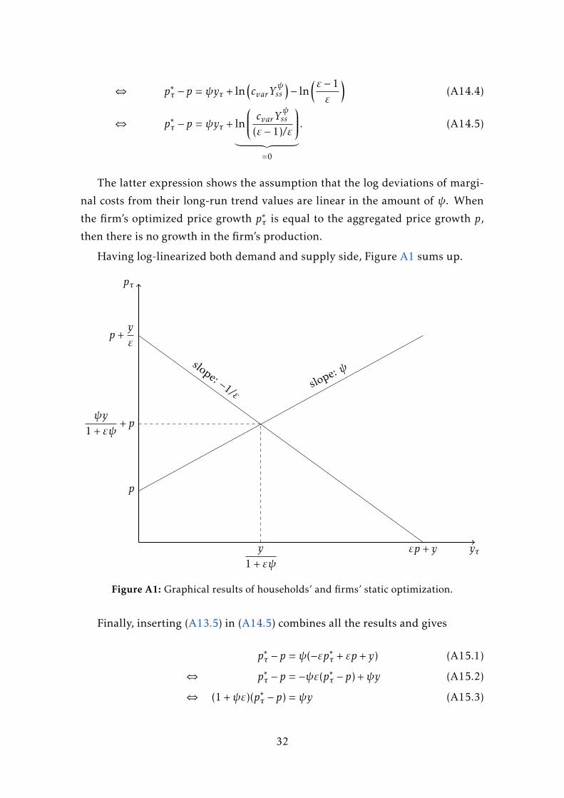
The latter expression shows the assumption that the log deviations of margi-

nal costs from their long-run trend values are linear in the amount of ψ. When

the firm’s optimized price growth p∗τ is equal to the aggregated price growth p,

then there is no growth in the firm’s production.

Having log-linearized both demand and supply side, Figure A1 sums up.

yτ

pτ

p

slope: ψ

p+y

ε

εp+ y

slope: −1/ε

ψy

1 + εψ+ p

y

1 + εψ

Figure A1: Graphical results of households’ and firms’ static optimization.

Finally, inserting (A13.5) in (A14.5) combines all the results and gives

p∗τ − p = ψ(−εp∗τ + εp+ y) (A15.1)

⇔ p∗τ − p = −ψε(p∗τ − p) +ψy (A15.2)

⇔ (1 +ψε)(p∗τ − p) = ψy (A15.3)

32

⇔ p∗τ − p =(

ψ

1 +ψε

)y. (A15.4)

A.4 Calvo Pricing – Calculation Steps

Dividing the first-order condition by 2k, using the fact that xt is t-measurable,

and expanding the sum gives

∞∑j=0

(βφ)jxt −∞∑j=0

(βφ)jEtp∗t+j = 0. (A16)

Excluding xt from the sum, using the formula for an infinite geometric series,

and multiplying by (1− βφ) gives

xt = (1− βφ)∞∑j=0

(βφ)jEtp∗t+j . (A17)

Again, using t-measurability (Etp∗t = p∗t) and excluding the first summand pro-

vides a sum from j = 1 to infinity that can be substituted in a subsequent step:

xt = (1− βφ)

∞∑j=1

(βφ)jEtp∗t+j + p∗t

. (A18)

Furthermore, Eq.(A17) can be rewritten for t+ 1 (since firms optimize in each

period),

Etxt+1 = (1− βφ)∞∑j=1

(βφ)j−1Etp∗t+j (A19.1)

⇔ βφEtxt+1 = (1− βφ)∞∑j=1

(βφ)jEtp∗t+j , (A19.2)

for eliminating the sum in (A18):

xt = βφEtxt+1 + (1− βφ)p∗t . (A20)

Inserting condition (11) leads to the expression

pt −φpt−1

1−φ= βφ

Etpt+1 −φpt1−φ

+ (1− βφ)p∗t (A21.1)

33

⇔ pt −φpt−1 = βφ(Etpt+1 −φpt) + (1−φ)(1− βφ)p∗t , (A21.2)

that only contains parameters and variants of the variable p. Then, with the

definition of (A10) and first-order Taylor expansion, the inflation rate π can be

expressed through differences of p. In the same way, the conditional expectation

value for period t + 1 can be expressed with

Etpt+1 − pt ≈ Etπt+1. (A22)

Since this approximation is sufficiently exact for small values of π, an equality

sign will be used for all following calculations. Now (A21.2) can be rearranged

to insert approximations π and Eq.(A22):

φ(pt − pt−1) = βφ(Etpt+1 −φpt) + (1−φ)(1− βφ)p∗t − (1−φ)pt (A23.1)

⇔ πt = βEtπt+1 +(1−φ)(1− βφ)

φp∗t −

1−φφ

pt + β(1−φ)pt. (A23.2)

A.5 Intertemporal Optimization – Calculation Steps

The optimization problem has the constraint

Ct · Pt +Bt+1 =Wt + (1 + it−1) ·Bt, (A24)

where W is the nominal wage and B the nominal value of bonds. The latter pro-

vides the link between two periods. Depending on the definition of the interest

rate, the period can vary. Here it has been chosen in a way so that the interest

from period t enters the Euler condition. Dynamic Programming uses the addi-

tively separable utility function and the envelope theorem to set up optimality

conditions for two consecutive periods. The procedure can be divided into three

parts. The first part is to write a value function, the Bellman equation. Under the

assumption that the second term of the expanded utility

U (Ct) +Et

∞∑s=t+1

βs−t−1U (Cs)

(A25)

is maximized in period t, the Bellman equation is

V (Bt) ≡maxCt{U (Ct) + βV (Bt+1)} . (A26)

34

The expected value vanishes since Bt+1 is determined by variables in period t

in the constraint. Differentiating with respect to Ct gives the first-order condition

ddCt

U (Ct) + βddCt

V (Bt+1) =U ′(Ct) + βV ′(Bt+1) · dBt+1

dCt= 0, (A27)

which results in

U ′(Ct) = PtβV′(Bt+1). (A28)

Eq.(A28) relates the marginal utility to the marginal value in the following

period, the time preference, and prices in the same period. Therefore, a higher β

and Pt results in a lower Ct.

In the next part, the envelope theorem is used to differentiate the value func-

tion (by inserting the optimized C∗t ) with respect to the costate variable Bt:

V (Bt) =U (C∗t ) + βV (Bt+1) (A29.1)

⇒ dVdBt

=βV ′(Bt+1) · dBt+1

dBt(A29.2)

⇔ V ′(Bt)=βV′(Bt+1) · (1 + it−1). (A29.3)

Eq.(A29.3) reveals the relationship of the marginal value functions.

In a third and last step, the first-order condition (A28) can be used to replace

the value functions in Eq.(A29.3) with the marginal utility in both periods t and

t − 1:

U ′(Ct−1)Pt−1β

=β · U′(Ct)Ptβ

· (1 + it−1) (A30.1)

⇒ U ′(Ct)Pt

=β(1 + it)Et

[U ′(Ct+1)Pt+1

]. (A30.2)

The time shift yields the Euler condition.

A.6 Jensen’s Inequality – Calculation Steps

f (EX) ≥ E[f (X)] holds for concave functions, i.e. the logarithm and Jensen’s in-

equality still holds for the conditional expected value. Since the function’s cur-

vature is sufficiently small, the accuracy is comparable to log-linearization for

small growth rates. Moreover, the exactness increases for larger values because

35

of (ln(x))′′ → 0 for increasing x. However, resulting values will always be under-

estimated.

lnEt

[Zt+1

Zt

]= lnEt

[exp

(ln

(Zt+1

Zt

))]≈ lnEt

[1 + ln

(Zt+1

Zt

)](A31.1)

= ln(1 +Et

[ln

(Zt+1

Zt

)])≈ Et

[ln

(Zt+1

Zt

)]. (A31.2)

A.7 Second-Order Taylor Approximation

The Taylor series (in R) helps in finding a polynomial to substitute a certain func-

tion f (x) (i.e. exponential, logarithm, etc.) around a point x0. The generalized

formula of the degree n in the compact sigma notation is

T aylor(n) =n∑j=0

f (j)(x0)j!

(x − x0)j , (A32)

where f (j) denotes the jth derivative with f (0) = f as a special case. Thereby,

larger values for n give better approximations of the original function f (x). In

(23.1), f (x) = ln(1 + x) and n = 2. Formula (A32) simplifies to

T aylor(2) = ln(1 + x0) +1

1 + x0(x − x0)− 1

2(1 + x0)2 (x − x0)2. (A33)

The result in (23.1) appears with x0 = 0 and yt+1 (πt+1 respectively) as the

argument of the function:

ln(1 + yt+1) ≈ yt+1 −12yt+1

2. (A34)

A.8 Standard Targeting Rule – Calculation Steps

The Lagrangian has to be differentiated with respect to yt, πt, and it, since the

central bank sets the nominal interest rate:

L (πt, yt, it) = Et

∞∑s=t

βs−t(π2s + δys

2)−χs(πs − βπs+1 −κys)

−ϕs(ys − ys+1 +

1σ

(is − r −πs+1) +1

2σπ2s+1 +

12ys+1

2). (A35)

36

First-order conditions:

∂L∂πt

= 2πt −χt = 0 (A36.1)

∂L∂yt

= 2δyt +χtκ −ϕt(1 + yt −Etyt+1) = 0 (A36.2)

∂L∂it

= −ϕtσ

= 0. (A36.3)

Condition (A36.2) follows with Eq.(27). From condition (A36.3) follows that

ϕt = 0, hence the minimized loss will not change if the IS curve shifts, as the

central bank can counteract it one by one through resetting the nominal interest

rate. Combining (A36.1) and (A36.2), the standard targeting rule under discre-

tion arises.

A.9 Optimal Interest Rate for Positive Inflation Targets

When the Lagrangian attains the “leaning against the wind” condition, it is ex-

tended with π∗ (as in (29), the loss function). Therefore, the standard targeting

rule changes to

πt −π∗ = −δκyt, (A37)

whereby the optimal output gap,

yt = −βκ

δ+κ2Etπt+1 +π∗κ

δ+κ2 , (A38)

comprises an additional term. After inserting (A38) in the IS curve, the interest

rule also has an additional (negative) term. This would lead to a generally lower

interest level.

A.10 Equilibrium Condition – Calculation Steps

Eq.(51) and Eq.(52) in more detail:

Et(yt+1 − yt)2 = Et[((−κθ) (µet + ζt+1)− (−κθ)et)

2]

(A39.1)

= Et[(−κθ)2 (µet + ζt+1 − et)2

](A39.2)

= (−κθ)2Et[((µ− 1)et + ζt+1)2

](A39.3)

= ((−κθ)(µ− 1))2 e2t + (−κθ)2

(V artζt+1 + (Etζt+1)2

)(A39.4)

37

= κ2θ2(µ− 1)2e2t +κ2θ2σ2

e (A39.5)

= (κθ)2((1−µ)2e2

t + σ2e

)(A39.6)

and

it = r +αµet −12

(δθ)2(µ2e2

t + σ2e

)− σ

2(κθ)2

((1−µ)2e2

t + σ2e

)+ σut (A40.1)

= r +αµet −12

((δθ)2µ2e2

t + (δθ)2σ2e + σ (κθ)2(1−µ)2e2

t + σ (κθ)2σ2e

)+ σut (A40.2)

= r +αµet −12

(((1−µ)2σκ2 +µ2δ2

)θ2e2

t +(σκ2 + δ2

)θ2σ2

e

)+ σut. (A40.3)

A.11 Parameter Discussion

Eq.(45) includes all parameters of the model.43 This subsection gives a brief

overview over possible values, which are used to graphically depict the equi-

librium conditions.

The discount parameter β is typically close to 1. Galı (2015, 67) and Rotem-

berg and Woodford (1997, 321) set β equal to 0.99 (quarterly), whereas Jensen

(2002, 939) uses this under an annual interpretation. Walsh (2010, 362) also sets

it to 0.99. Galı and Gertler (1999, 207) estimate a value of 0.988. To keep the

framework close to the actual interest setting of the central bank, all calculations

are carried out quarterly and β will be set to 0.99.

The slope of the NKPC κ takes values close to zero and usually lower than 1.

Roberts (1995, 982) estimates in his original NKPC article κ ≈ 0.3. On a quarterly

basis, Walsh (2010, 362) sets 0.05, Galı and Gertler (1999, 13) estimate 0.02, and

McCallum and Nelson (2004, 47) suggest 0.01−0.05. Jensen (2002, 939) calibrates

an annual value of 0.142, whereas Clarida et al. (2000, 170) set 0.3 (yearly) and

give a range of 0.05 to 1.22 in the literature. In the baseline simulation, κ is set to

0.04.44

Woodford (2003a, 165) states that a value of 1 is customary in the RBC liter-

ature for σ , the multiplicative inverse of the IES (see, e.g. Clarida et al. (2000,

170), Galı (2015, 67), Yun (1996, 359)). A slightly larger value (1.5) is set by

Jensen (2002, 939) and Smets and Wouters (2003, 1143) estimate 1.4. An insight-

ful metadata study by Havranek et al. (2015) estimates a mean IES of 0.5 (σ = 2)43Note that variances σ2

e and σ2u are only indirectly included.

44Note that this implies κ = 0.16 on a yearly basis.

38

across all countries. However, they report that more developed countries have a

higher IES (lower σ ). Therefore, σ will be set to 1.

The weight on output fluctuations δ is set to 0.25 in almost all the literature

(see, e.g. Walsh (2010, 362), 939), McCallum and Nelson (2004, 47), Jensen (2002,

939)). The latter reports values from 0.05 to 0.33 in other papers. Thus, δ = 0.25

will also be assumed for the simulation.

Walsh (2003, 275) allows values up to 0.7 for µ, the cost shock persistence.

Clarida et al. (2000, 170) set 0.27 (yearly) and Galı and Rabanal (2004, 48) esti-

mate 0.95. Generally, Smets and Wouters (2003, 1142–1143) estimate persisten-

cies of 0.8 and higher, which is confirmed by Smets and Wouters (2007). Thus,

µ will be treated as a variable in the range of 0.6 − 0.85. The smallest value 0.6

implies 0.1296 on an annual basis.

For the standard deviation of a cost shock, Sims (2011, 17) sets 0.01 (σ2e =

0.0001), Jensen (2002, 939) sets 0.015 (σ2e = 0.000225), and Galı and Rabanal

(2004, 48) estimate 0.011 (σ2e = 0.000121). McCallum and Nelson (2004, 47) set

an annualized standard deviation of 0.02 (σ2e = 0.0004). The conservative value

of 0.0001 will be taken for the simulation.

39

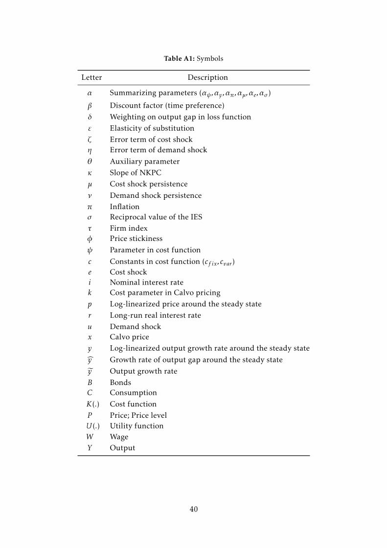
Table A1: Symbols

Letter Description

α Summarizing parameters (αψ,αy ,απ,αµ,αe,ασ )

β Discount factor (time preference)δ Weighting on output gap in loss functionε Elasticity of substitutionζ Error term of cost shockη Error term of demand shock

θ Auxiliary parameterκ Slope of NKPCµ Cost shock persistence

ν Demand shock persistenceπ Inflationσ Reciprocal value of the IESτ Firm indexφ Price stickinessψ Parameter in cost function

c Constants in cost function (cf ix, cvar)e Cost shocki Nominal interest ratek Cost parameter in Calvo pricingp Log-linearized price around the steady stater Long-run real interest rateu Demand shockx Calvo pricey Log-linearized output growth rate around the steady state

y Growth rate of output gap around the steady statey Output growth rateB BondsC ConsumptionK(.) Cost functionP Price; Price levelU (.) Utility functionW WageY Output

40