Equilibrium Conditions for the SimpleNew Keynesian Model

Lawrence J. Christiano

August 24, 2014

• Baseline NK model with no capital and with a competitivelabor market.

— private sector equilibrium conditions— Details: http://faculty.wcas.northwestern.edu/~lchrist/course/Korea_2012/intro_NK.pdf

• Use the equilibrium conditions of this model:

— as a base to introduce financial frictions— to illustrate the application of solution methods.

Households

• Problem:

max E

0

•

Ât=0

bt

log C

t

− exp (tt

)N

1+jt

1+ j

!, t

t

= ltt−1

+ #tt

s.t. P

t

C

t

+ B

t+1

≤ W

t

N

t

+ R

t−1

B

t

+ Profits net of taxest

• First order conditions:

1

C

t

= bE

t

1

C

t+1

R

t

¯pt+1

(5)

exp (tt

)C

t

N

jt

=W

t

P

t

.

Goods Production• A homogeneous final good is produced using the following(Dixit-Stiglitz) production function:

Y

t

=

#Z1

0

Y

#−1

#i,t

dj

% ##−1

.

• Each intermediate good, Y

i,t

, is produced as follows:

Y

i,t

=

=exp(at

)z}|{A

t

N

i,t

, a

t

= ra

t−1

+ #a

t

• Before discussing the firms that operate these productionfunctions, we briefly investigate the socially e¢cient (‘FirstBest’) allocation of labor across i, for given N

t

:

N

t

=Z

1

0

N

it

di

E¢cient Sectoral Allocation of Labor• With Dixit-Stiglitz final good production function, there is asocially optimal allocation of resources to all the intermediateactivities, Y

i,t

— It is optimal to run them all at the same rate, i.e., Y

i,t

= Y

j,t

for all i, j 2 [0, 1] .

• For given N

t

, it is optimal to set N

i,t

= N

j,t

for all i, j 2 [0, 1]

• In this case, final output is given by

Y

t

= e

a

t

N

t

.

• Best way to see this is to suppose that labor is not allocatedequally to all activities.— But, this can happen in a million di§erent ways when there is acontinuum of inputs!

— Explore one simple deviation from N

i,t

= N

j,t

for all i, j 2 [0, 1] .

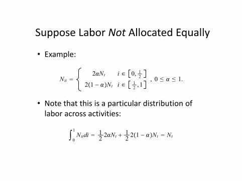
Suppose�Labor�Not Allocated�Equally

• Example:

• Note�that�this�is�a�particular�distribution�of�labor�across�activities:

Nit �2)Nt i � 0, 12

2�1 " ) Nt i � 12 , 1

, 0 t ) t 1.

;0

1Nitdi � 1

2 2)Nt �12 2�1 " ) Nt � Nt

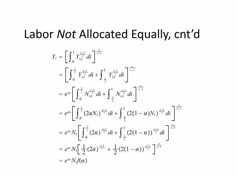
Labor�Not Allocated�Equally,�cnt’dYt � ;

0

1Yi,t

/"1/ di

//"1

� ;0

12 Yi,t

/"1/ di � ;

12

1Yi,t

/"1/ di

//"1

� eat ;0

12 Ni,t

/"1/ di � ;

12

1Ni,t

/"1/ di

//"1

� eat ;0

12 �2)Nt 

/"1/ di � ;

12

1�2�1 " ) Nt 

/"1/ di

//"1

� eatNt ;0

12 �2) 

/"1/ di � ;

12

1�2�1 " )  

/"1/ di

//"1

� eatNt 12 �2) /"1/ � 12 �2�1 " )  

/"1/

//"1

� eatNtf�) 

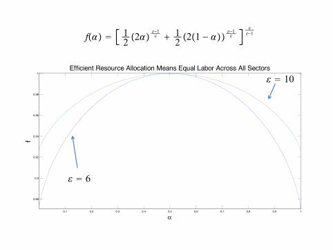
0.1 0.2 0.3 0.4 0.5 0.6 0.7 0.8 0.9 1

0.88

0.9

0.92

0.94

0.96

0.98

1

D

f

Efficient Resource Allocation Means Equal Labor Across All Sectors

/ � 6

/ � 10

f�)  � 12 �2) 

/"1/ � 12 �2�1 " )  

/"1/

//"1

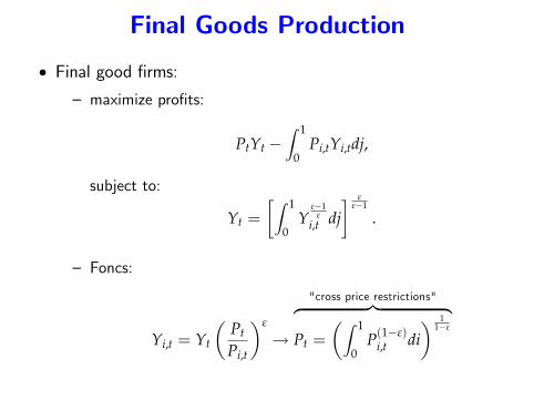
Final Goods Production

• Final good firms:

— maximize profits:

P

t

Y

t

−Z

1

0

P

i,t

Y

i,t

dj,

subject to:

Y

t

=

#Z1

0

Y

#−1

#i,t

dj

% ##−1

.

— Foncs:

Y

i,t

= Y

t

*P

t

P

i,t

+#

!

"cross price restrictions"z }| {

P

t

=

*Z1

0

P

(1−#)i,t

di

+ 1

1−#

Intermediate Goods Production• Demand curve for i

th monopolist:

Y

i,t

= Y

t

*P

t

P

i,t

+#

.

• Production function:

Y

i,t

= exp (at

)N

i,t

, a

t

= ra

t−1

+ #a

t

• Calvo Price-Setting Friction:

P

i,t

=

,˜

P

t

with probability 1− qP

i,t−1

with probability q .

• Real marginal cost:

s

t

=dCost

dworkerdoutputdworker

=

minimize monopoly distortion by setting = #−1

#z }| {(1− n) W

t

P

t

exp (at

)

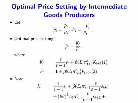
Optimal Price Setting by IntermediateGoods Producers

• Let

˜

p

t

≡˜

P

t

P

t

,

¯pt

≡P

t

P

t−1

.

• Optimal price setting:

˜

p

t

=K

t

F

t

,

where

K

t

=#

#− 1

s

t

+ bqE

t

¯p#t+1

K

t+1

(1)

F

t

= 1+ bqE

t

¯p#−1

t+1

F

t+1

.(2)

• Note:

K

t

=#

#− 1

s

t

+ bqE

t

¯p#t+1

#

#− 1

s

t+1

+ (bq)2 E

t

¯p#t+2

#

#− 1

s

t+2

+ ...

Goods and Price Equilibrium Conditions• Cross-price restrictions imply, given the Calvo price-stickiness:

P

t

=h(1− q) ˜

P

(1−#)t

+ qP

(1−#)t−1

i 1

1−#.

• Dividing latter by P

t

and solving:

˜

p

t

=

"1− q ¯p#−1

t

1− q

# 1

1−#

!K

t

F

t

=

"1− q ¯p#−1

t

1− q

# 1

1−#

(3)

• Relationship between aggregate output and aggregate inputs:

C

t

= p

∗t

A

t

N

t

, (6)

where p

∗t

=

2

4(1− q)

1− q ¯p

(#−1)t

1− q

! ##−1

+ q¯p#

t

p

∗t−1

3

5−1

(4)

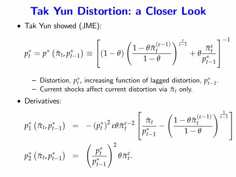
Tak Yun Distortion: a Closer Look• Tak Yun showed (JME):

p

∗t

= p

∗ 5¯p

t

, p

∗t−1

6≡

2

4(1− q)

1− q ¯p

(#−1)t

1− q

! ##−1

+ q¯p#

t

p

∗t−1

3

5−1

— Distortion, p

∗t

, increasing function of lagged distortion, p

∗t−1

.— Current shocks a§ect current distortion via ¯p

t

only.

• Derivatives:

p

∗1

5¯p

t

, p

∗t−1

6= − (p∗

t

)2 #q ¯p#−2

t

2

4 ¯pt

p

∗t−1

−

1− q ¯p

(#−1)t

1− q

! 1

#−1

3

5

p

∗2

5¯p

t

, p

∗t−1

6=

p

∗t

p

∗t−1

!2

q ¯p#t

.

Linear Expansion of Tak Yun Distortion inUndistorted Steady State

• Linearizing about ¯pt

= ¯p, p

∗t−1

= p

∗:

dp

∗t

= p

∗1

( ¯p, p

∗) d

¯pt

+ p

∗2

( ¯p, p

∗) dp

∗t−1

,

where dx

t

≡ x

t

− x, for x

t

= p

∗t

, p

∗t−1

,

¯pt

.

• In an undistorted steady state (i.e., ¯pt

= p

∗t

= p

∗t−1

= 1) :

p

∗1

(1, 1) = 0, p

∗1

(1, 1) = q.

so that

dp

∗t

= 0× d

¯pt

+ qdp

∗t−1

! p

∗t

= 1− q + qp

∗t−1

• Often, people that linearize NK model ignore p

∗t

.

— Reflects that they linearize the model around aprice-undistorted steady state.

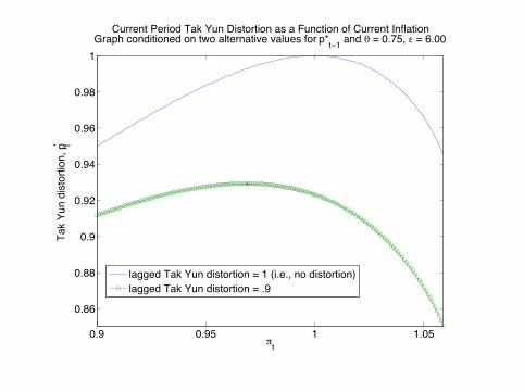
0.9 0.95 1 1.05

0.86

0.88

0.9

0.92

0.94

0.96

0.98

1

πt

Tak

Yun

dist

ortio

n, p* t

Current Period Tak Yun Distortion as a Function of Current InflationGraph conditioned on two alternative values for p*t−1 and θ = 0.75, ε = 6.00

lagged Tak Yun distortion = 1 (i.e., no distortion)lagged Tak Yun distortion = .9

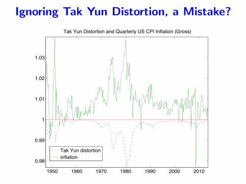
Ignoring Tak Yun Distortion, a Mistake?

1950 1960 1970 1980 1990 2000 2010

0.98

0.99

1

1.01

1.02

1.03

Tak Yun Distortion and Quarterly US CPI Inflation (Gross)

Tak Yun distortioninflation

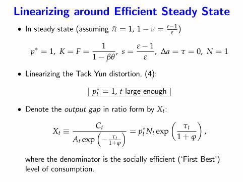
Linearizing around E¢cient Steady State• In steady state (assuming ¯p = 1, 1− n = #−1

# )

p

∗ = 1, K = F =1

1− bq, s =

#− 1

#, Da = t = 0, N = 1

• Linearizing the Tack Yun distortion, (4):

p

∗t

= 1, t large enough

• Denote the output gap in ratio form by X

t

:

X

t

≡C

t

A

t

exp

7− t

t

1+j

8 = p

∗t

N

t

exp

*t

t

1+ j

+,

where the denominator is the socially e¢cient (‘First Best’)level of consumption.

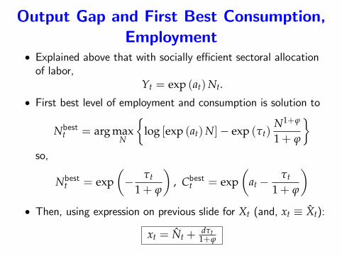
Output Gap and First Best Consumption,Employment

• Explained above that with socially e¢cient sectoral allocationof labor,

Y

t

= exp (at

)N

t

.

• First best level of employment and consumption is solution to

N

bestt

= arg max

N

,log [exp (a

t

)N]− exp (tt

)N

1+j

1+ j

9

so,

N

bestt

= exp

*−

tt

1+ j

+, C

bestt

= exp

*a

t

−t

t

1+ j

+

• Then, using expression on previous slide for X

t

(and, x

t

≡ ˆ

X

t

):

x

t

= ˆ

N

t

+ dtt

1+j

NK IS Curve, Baseline Model• The intertemporal Euler equation, (5), after substituting for C

t

in terms of X

t

:1

X

t

A

t

exp

7− t

t

1+j

8 = bE

t

1

X

t+1

A

t+1

exp

7− t

t+1

1+j

8 R

t

¯pt+1

1

X

t

= E

t

1

X

t+1

R

∗t+1

R

t

¯pt+1

,

where

R

∗t+1

≡1

bexp

*a

t+1

− a

t

−t

t+1

− tt

1+ j

+

then, use

dz

t

u

t

= ˆ

z

t

+ ˆ

u

t

,

\*u

t

z

t

+= ˆ

u

t

− ˆ

z

t

to obtain:ˆ

X

t

= E

t

;ˆ

X

t+1

−5

ˆ

R

t

− b̄pt+1

− ˆ

R

∗t+1

6=

NK IS Curve, Baseline Model• We now want to establish (when the steady state is e¢cient)the following result:

E

t

5ˆ

R

t

− b̄pt+1

− ˆ

R

∗t+1

6

= r

t

− E

t

pt+1

− r

∗t

,

where

r

t

≡ log R

t

, r

∗t

≡ E

t

log R

∗t+1

, pt+1

≡ log

¯pt+1

.

• Note:

Z

t

= exp (zt

) , where z

t

≡ log Z

t

ˆ

Z

t

≡dZ

t

Z

=d exp (z

t

)

Z

=Zdz

t

Z

= dz

t

.

• The result follows easily from the following facts in e¢cientsteady state:

log R

∗ = log R, log

¯p = 0.

NK IS Curve, Baseline Model

• Substituting

ˆ

X

t

= E

t

;ˆ

X

t+1

−5

ˆ

R

t

− b̄pt+1

− ˆ

R

∗t+1

6=, x

t

≡ ˆ

X

t

,

we obtain NK IS curve:

x

t

= E

t

x

t+1

− E

t

[rt

− pt+1

− r

∗t

]

• Also,

r

∗t

= − log (b) + E

t

#a

t+1

− a

t

−t

t+1

− tt

1+ j

%.

Linearized Marginal Cost in Baseline Model

• Marginal cost (using da

t

= a

t

, dtt

= tt

because a = t = 0):

s

t

= (1− n)¯

w

t

A

t

,

¯

w

t

= exp (tt

)N

jt

C

t

! b̄w

t

= tt

+ a

t

+ (1+ j) ˆ

N

t

• Then,

ˆ

s

t

= b̄wt

− a

t

= (j+ 1)h

tt

j+1

+ ˆ

N

t

i= (j+ 1) x

t

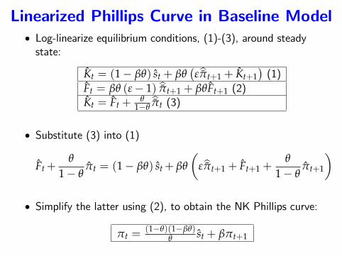
Linearized Phillips Curve in Baseline Model• Log-linearize equilibrium conditions, (1)-(3), around steadystate:

ˆ

K

t

= (1− bq) ˆ

s

t

+ bq5# b̄p

t+1

+ ˆ

K

t+1

6(1)

ˆ

F

t

= bq (#− 1) b̄pt+1

+ bq ˆ

F

t+1

(2)ˆ

K

t

= ˆ

F

t

+ q1−qb̄p

t

(3)

• Substitute (3) into (1)

ˆ

F

t

+q

1− qˆp

t

= (1− bq) ˆ

s

t

+ bq

*# b̄p

t+1

+ ˆ

F

t+1

+q

1− qˆp

t+1

+

• Simplify the latter using (2), to obtain the NK Phillips curve:

pt

= (1−q)(1−bq)q ˆ

s

t

+ bpt+1

The Linearized Private Sector EquilibriumConditions

x

t

= x

t+1

− [rt

− pt+1

− r

∗t

]

pt

= (1−q)(1−bq)q ˆ

s

t

+ bpt+1

ˆ

s

t

= (j+ 1) x

t

r

∗t

= − log (b) + E

t

ha

t+1

− a

t

− tt+1

−tt

1+j

i

Nonlinear Private Sector EquilibriumConditions

K

t

=#

#− 1

s

t

+ bqE

t

¯p#t+1

K

t+1

(1)

F

t

= 1+ bqE

t

¯p#−1

t+1

F

t+1

.(2)

K

t

F

t

=

"1− q ¯p#−1

t

1− q

# 1

1−#

(3)

p

∗t

=

2

4(1− q)

1− q ¯p

(#−1)t

1− q

! ##−1

+ q¯p#

t

p

∗t−1

3

5−1

(4)

1

C

t

= bE

t

1

C

t+1

R

t

¯pt+1

(5)

C

t

= p

∗t

A

t

N

t

. (6)