calibration and performances of in-situ gamma ray...
TRANSCRIPT

0
Calibration and performances of in-situ gamma ray spectrometer
by
Manjola Shyti
Submitted to
The University of Ferrara
(Faculty of Mathematics, Physics and Natural Sciences)
for the degree of
PhD in Physics
March 2013
Ferrara, Italy: 22, March 2013

1
Table of contents
Abstract .............................................................................................................................................. 8
Chapter 1 .......................................................................................................................................... 12
1. Introduction to environmental radioactivity ............................................................................... 13
1.1 Law of radioactive decay ................................................................................................... 13
1.2 The statistical nature of radioactive decay ....................................................................... 17
1.3 Radioactive decay and decay modes ................................................................................ 19
1.3.1 Alpha decay ..................................................................................................................... 22
1.3.2 Beta decay ....................................................................................................................... 24
1.3.3 Gamma decay.................................................................................................................. 26
1.4 Sources of radioactivity ..................................................................................................... 27
1.4.1 Cosmic radiation .............................................................................................................. 28
1.4.2 Primordial radionuclides ................................................................................................. 29
1.4.3 Man-made radionuclides ................................................................................................ 35
Chapter 2 .......................................................................................................................................... 37
2. Gamma-ray spectrometry and principles of gamma ray detectors ............................................. 37
2.1 Photoelectric effect ........................................................................................................... 37
2.2 Compton scattering ........................................................................................................... 39
2.3 Pair production .................................................................................................................. 40
2.4 The probability interaction and correction of gamma radiation ..................................... 41
2.5 Properties of gamma ray spectra ...................................................................................... 44
2.6 Principles of gamma ray detectors ................................................................................... 47
2.7 Scintillation detector features .......................................................................................... 51
2.8 Semiconductor detectors features ................................................................................... 56
Chapter 3 .......................................................................................................................................... 59
3. Campaign activity ......................................................................................................................... 59
3.1 Study area .......................................................................................................................... 59
3.2 A portable gamma-ray spectrometer: ZaNaI_1.0L ........................................................... 65
3.3 In-situ spectrum acquisition .............................................................................................. 73
3.4 Soil sampling ...................................................................................................................... 76
Chapter 4 .......................................................................................................................................... 79
2
4. Laboratory activity ....................................................................................................................... 79
4.1 Preparation of samples ..................................................................................................... 79
4.2 High resolution gamma-ray spectrometry using the MCA_Rad system ......................... 80
Chapter 5 .......................................................................................................................................... 86
5. Discussion of obtained results ..................................................................................................... 86
5.1 Spectrum analysis .............................................................................................................. 86
5.2 Soil sample data: statistical analysis ................................................................................. 87
5.3 Study of performances of in-situ gamma-ray measurements ......................................... 89
5.3.1 Correlation between in-situ acquisition on ground and laboratory measurements ....... 91
5.3.2 Correlation between in-situ acquisition on tripod and laboratory measurements ......... 93
5.3.3 Correlation between in-situ acquisition on ground and on tripod .................................. 96
5.3.4 Correlation between in-situ acquisition on ground and on operator shoulder ............... 99
5.3.5 Interference of vegetative cover for-situ acquisition on ground and on operator shoulder
................................................................................................................................................ 102
Chapter 6 ........................................................................................................................................ 105
6. Conclusions................................................................................................................................. 105
References ...................................................................................................................................... 109

3
List of figures and tables
Chapter 1
Figure 1.1: exponential decay of activity.
Figure 1.2: temporal trend of the number of parent atoms and daughter atoms in a radioactive sample.
Figure 1.3: qualitative representation of the secular equilibrium concept. The atoms of 238U subject to decay are
represented as a fluid which is poured into the container of 234Th. In secular equilibrium conditions the outgoing flow
from the container of 234Th, corresponding to the number of atoms of 234Th subject to decay, will be equal to the
incoming flow, corresponding to the number of atoms of 234Th produced by the decay of 238U. If the decay chain of 238U
is in secular equilibrium in its entirety, equality between the incoming and the out coming flow is valid for every element
in the chain.
Figure 1.4: example of three Poisson distributions with mean value equal to 1, 5 and 10. It is observed that as average
value increase, the Poisson distribution is close to Gauss ones.
Figure 1.5: binding energy per nucleon of common isotopes.
Figure 1.6: representation of the stable nuclei, marked with green squares, as a function of the atomic number Z. The
stable nuclei are arranged on the straight line Z = N for values of Z less than 20; for Z > 20, the stability curve towards
the axis N, highlighting the greater stability of the nuclei with a number of neutrons greater than the number of protons.
Figure 1.7: three dimensional representation of valley of stability.
Figure 1.8: schematic representation of decay and - decay of 227Th.
Figure 1.9: alpha spectrum associated with the decay of 227Th.
Figure 1.10: schematic representation of β- decay; β− (on the left) and β+ (on the right).
Figure 1.11: schematic representation decay for 137Cs.
Figure 1.12: schematic representation of electron capture process.
Figure 1.13: representation of the reactions involved in the interaction of particles of primary cosmic rays with the
atmosphere, giving rise to secondary cosmic rays.
Figure 1.14: potassium decay modes.
Figure 1.15: uranium decay chain.
Figure 1.16: thorium decay chain.
Figure 1.17: decay chain of 238U where are highlighted the possible points in which the condition of secular equilibrium
is broken.
Figure 1.18: decay chain of 232Th where are highlighted the possible points in which the condition of personal
equilibrium is broken.
Table 1.1: ranges and averages of the concentrations of 238U, 232Th, and 40K in typical rocks and soils

4
Chapter 2
Figure 2.1: schematic representation of the photoelectric effect and the subsequent emission of X-ray characteristic.
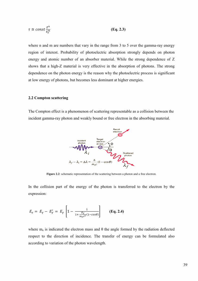
Figure 2.2: schematic representation of the scattering between a photon and a free electron.
Figure 2.3: schematic of the Compton scattering process.
Figure 2.4: cross section for the photoelectric effect, Compton scattering and pair production and the total cross section
for an atom of Lead as a function of the photon energy.
Figure 2.5: gamma ray emission line spectra of potassium (IAEA-TECDOC-1363, 2003).
Figure 2.6: gamma ray emission line spectra of uranium (IAEA-TECDOC-1363, 2003).
Figure 2.7: gamma ray emission line spectra of thorium (IAEA-TECDOC-1363, 2003).
Figure 2.8: simulated potassium fluence rates at 300 meter height (IAEA-TECDOC-1363, 2003).
Figure 2.9: simulated uranium fluence rates at 300 meter height (IAEA-TECDOC-1363, 2003).
Figure 2.10: simulated thorium fluence rates at 300 meter height (IAEA-TECDOC-1363, 2003).
Figure 2.11: example of energy resolution for a gamma rays spectrometer (IAEA-TECDOC-1363, 2003).
Figure 2.12: schematic representation of a scintillation detector.
Figure 2.13: schematic representation of the energy levels of singlet and triplet in organic scintillators.
Figure 2.14: schematic representation of the band structure of an inorganic scintillator. The centers activators introduce
energy levels within the energy gap between the valence band and the conduction band.
Figure 2.15: dependence of the light emission of scintillating crystals by temperature.
Figure 2.16: scheme of a photomultiplier coupled to a scintillator.
Figure 2.17: schematic representation of a p-n junction.
Chapter 3
Figure 3.1: framework of the basin of Ombrone in respect to Tuscany region.
Figure 3.2: geological map of the Basin of Ombrone River 1:500000 highlighted with the points in which were carried
out the measurements of natural radioactivity.
Figure 3.3: geological map of the commune of Schio.
Figure 3.4: coordinate system used in the theoretical calculations for the variation of detector count rate with its height
respect to the ground.
Figure 3.5: percentage contribution of the signal received by the detector placed at a height of 0.05 m.
Figure 3.6: percentage contribution of the signal received by the detector placed at a height of 0.5 m.
Figure 3.7: percentage contribution of the signal received by the detector placed at a height of 1 m.

5
Figure 3.8: the ZaNaI_1.0Lsystem configuration set-up in a backpack.
Figure 3.9: energy windows for the WAM analysis of a gamma spectrum.
Figure 3.10: the sensitive spectra obtained through the FSA with NNLS constraint.
Figure 3.11: example of acquisition of the spectrum with backpack placed on the ground.
Figure 3.12: example of acquisition of the spectrum with backpack placed on the tripod at 1 m height above the ground.
Figure 3.13: example of acquisition of the spectrum with backpack placed on the shoulders.
Figure 3.14: example of the soil samples arrangement with respect to the central point in which is realized the
measurement of gamma-ray spectroscopy in situ.
Table 3.1: typical concentrations of constructed pads used to calibrate in-situ gamma-ray spectrometers (IAEA 1990).
Table 3.2: standard gamma ray energy windows recommended for natural radioelement mapping.
Table 3.3: the average of the distribution of natural radioisotopes concentration. The errors correspond to one standard
deviation. The conversion factors from Bq/kg are obtained by (IAEA-TECDOC-1363, 2003): 1%=313 Bq/kg for
potassium, 1 ppm=13.25 Bq/kg for uranium and 1 ppm=4.06 Bq/kg for thorium.
Table 3.4: standard pedological parameters to define in the campaign.
Table 3.5: environmental parameters monitored during the in situ measurement.
Chapter 4
Figure 4.1: ventilated oven used to dry the soil samples.
Figure 4.2: soil samples ready to be analyzed with MCA_Rad system.
Figure 4.3: MCA_Rad system composed by two coupled HPGe detectors.
Figure 4.4: MCA_Rad system shielding of HPGe detectors composed by copper and lead.
Figure 4.5: MCA_Rad system background spectra (live time 100 h) without (red) and with (green) shielding showing a
reduction of two order of magnitudes.
Figure 4.6: absolute efficiency curve for the MCA_Rad system obtained by fitting the corrected values for coincidence
summing with equation 2.16. Apparent efficiencies of 152Eu (blue triangles) and 56Co (green squares) are also presented.
Figure 4.7: loader of samples and instrumentation for reading the bar code of MCA_Rad system.
Table 4.1: the features of two detectors used for design of MCA_Rad system (these values are measured by the
manufacturer).
Chapter 5
Figure 5.1: representation of the total measured spectrum obtained by the superposition of the fundamental spectra of
cesium, potassium, uranium and thorium, and the background spectrum.

6
Figure 5.2: frequency histogram of the abundances of 40K obtained for the 400 soil sampling fitted with a log-normal
function.
Figure 5.3: the correlation between the abundance of K measured on sample using HPGe detectors and the abundance of
K measured in-situ using ZaNaI_1.0L placed on the ground is described by the relationship KZaNaI = (1.16 ± 0.05) KHPGe
with r2 = 0.90.
Figure 5.4: the correlation between the abundance of eU measured on sample using HPGe detectors and the abundance
of eU measured in-situ using ZaNaI_1.0L placed on the ground is described by the relationship eUZaNaI = (0.85 ± 0.11)
eUHPGe with r2 = 0.64.
Figure 5.5: the correlation between the abundance of eTh measured on sample using HPGe detectors and the abundance
of eTh measured in-situ using ZaNaI_1.0L placed on the ground is described by the relationship eThZaNaI = (0.97 ± 0.12)
eThHPGe with r2 = 0.80.
Figure 5.6: the correlation between the abundance of K measured on sample using HPGe detectors and the abundance of
K measured in-situ using ZaNaI_1.0L placed on the tripod is described by the relationship KZaNaI = (1.11 ± 0.05) KHPGe
with r2 = 0.88.
Figure 5.7: the correlation between the abundance of eU measured on sample using HPGe detectors and the abundance
of eU measured in-situ using ZaNaI_1.0L placed on the tripod is described by the relationship eUZaNaI = (0.75 ± 0.10)
eUHPGe with r2 = 0.66.
Figure 5.8: the correlation between the abundance of eTh measured on sample using HPGe detectors and the abundance
of eTh measured in-situ using ZaNaI_1.0L placed on the tripod is described by the relationship eThZaNaI = (0.92 ± 0.11)
eThHPGe with r2 = 0.79.
Figure 5.9: the correlation between the abundance of K measured by placing the ZaNaI_1.0L on ground and on tripod is
described by the relationship Kground= (0.93 ± 0.03) Ktripod with r2 = 0.98.
Figure 5.10: the correlation between the abundance of eU measured by placing the ZaNaI_1.0L on ground and on tripod
is described by the relationship eUground= (0.87 ± 0.03) eUtripod + (0.31 ± 0.14) with r2 = 0.73.
Figure 5.11: the correlation between the abundance of eTh measured by placing the ZaNaI_1.0L on ground and on tripod
is described by the relationship eThground= (0.94 ± 0.06) eThtripod with r2 = 0.96.
Figure 5.12: the correlation between the abundance of 137Cs measured by placing the ZaNaI_1.0L on ground and on
tripod is described by the relationship 137Csground= (0.81 ± 0.02) 137Cstripod with r2 = 0.95.
Figure 5.13: the correlation between the abundance of K measured by placing the ZaNaI_1.0L on ground and on
shoulder is described by the relationship Kground= (0.82 ± 0.01) Kshoulder + (0.08 ± 0.01) with r2 = 0.97.
Figure 5.14: the correlation between the abundance of eU measured by placing the ZaNaI_1.0L on ground and on
shoulder is described by the relationship eUground= (0.84 ± 0.01) eUshoulder + (0.13 ± 0.03) with r2 = 0.98.
Figure 5.15: the correlation between the abundance of eTh measured by placing the ZaNaI_1.0L on ground and on
shoulder is described by the relationship eThground= (0.83 ± 0.02) eThshoulder with r2 = 0.97.
Figure 5.16: the correlation between the abundance of 137Cs measured by placing the ZaNaI_1.0L on ground and on
shoulder is described by the relationship 137Csground= (0.77 ± 0.01) 137Csshoulder with r2 = 0.95.

7
Figure 5.17: for 0-50% vegetative cover case: the correlation between the abundance of Th measured by placing the
ZaNaI_1.0L on ground and on shoulder is described by the relationship Thground= (0.83 ± 0.02) Thshoulder with r2 = 0.99.
Figure 5.18: for 50-100% vegetative cover case: the correlation between the abundance of Th measured by placing the
ZaNaI_1.0L on ground and on shoulder is described by the relationship Thground= (0.85 ± 0.02) Thshoulder with r2 = 0.97.
Figure 5.19: for 0-50% vegetative cover case: the correlation between the abundance of 137Cs measured by placing the
ZaNaI_1.0L on ground and on shoulder is described by the relationship 137Csground= (0.72 ± 0.02) 137Csshoulder with r2 =
0.97.
Figure 5.20: for 50-100% vegetative cover case: the correlation between the abundance of 137Cs measured by placing
the ZaNaI_1.0L on ground and on shoulder is described by the relationship 137Csground= (0.77 ± 0.01) 137Csshoulder with r2 =
0.96.
Table 5.1: conversion factors between specific activity and concentrations of K, eU and eTh.
Table 5.2: relationships between the parameters of the distribution in the original scale and in that logarithmic one.
Table 5.3: the correlation parameters obtained for in-situ measurements on ground and laboratory measurements.
Table 5.4: correlation between measurements in-situ acquisition on tripod and in the laboratory.
Table 5.5: correlation parameters between in-situ measurements on ground and on tripod.
Table 5.6: correlation parameters between in-situ measurements on ground and on shoulder.
Table 5.7: correlation parameters between in-situ measurements on ground and on shoulder for two classes of vegetative
coverage.
Chapter 6
Table 6.1: correlation between ZaNaI_1.0L measurements obtained by placing the detector on ground and on tripod
respect to laboratory measurements.
Table 6.2: attenuation correction due to air for in-situ measurements at tripod (1m height).
Table 6.3: attenuation correction due to the presence of the operator during in-situ dynamics acquisition.
8
Abstract
Since 1896, when Henri Becquerel discovered that penetrating radiation was given off
in the radioactive decay of uranium, the studies on radioactivity have been an interest of
scientific world. With the spread of nuclear technologies applied to energy, health and
industrial production, the theme of environmental radioactivity monitoring increasingly is
becoming important to the policies of the health public protection both national and
European level. Italy is required to comply with the recommendation of the European
Commission of 8 June 2000 on the application of Article 36 of the Euratom Treaty
concerning the monitoring of levels of radioactivity in the environment for the purpose of
assessing the exposure of the population as a whole. In addition, the World Health
Organization has identified the first group of carcinogens gas 222
Rn, which is considered
the second leading cause, after smoking, of lung tumors. In our environment there are
various sources of radioactivity that can be natural or artificial origin. Gamma-ray
spectrometry is a widely used and powerful method that can be employed both to identify
and quantify radionuclides. The purpose of this work is calibration and performances of in
situ a portable gamma ray spectrometer.
In the first chapter I have given the necessary concepts for understanding the
phenomenon of radioactivity. Qualitatively has been described the process of radioactive
decay and its three types which can occur in nature. Three categories of environmental
radionuclides, cosmogenic, primordial and man-made are discussed. We are exposed to
environmental radiation from different sources. The origin of radioactivity in the
environment can be divided into two main sources: (a) natural and (b) man-made sources.
Mostly the naturally occurring radiation arises from terrestrial radioactive nuclides that are
widely distributed in the earth’s crust and extra-terrestrial sources arising from cosmic ray.
Also from human activities arise some other sources concerned with the use of radiation
and radioactive materials from which releases of radionuclides into the environment may
occur.
In the second chapter is described the gamma radiation interacts with matter via three
main processes: the photoelectric effect, Compton scattering and pair production The
operation of a detector is based on the interaction of photons constituting the incident
radiation with the material that constitutes the detector itself.. Thanks to these processes,
all or part of the energy possessed by the radiation is transferred to the mass of the detector

9
and then converted into an electrical signal. The basic notions related to the interaction of
electromagnetic radiation with matter that we will provide in this chapter will therefore be
useful to understand the mechanisms that are at the basis of the generation of a gamma
spectrum. In addition, this chapter will briefly describe the two main types of gamma
radiation detectors, i.e. the semiconductor detector and the scintillation, in particular the
high-pure germanium detector (HPGe) and a sodium iodide detector activated by thallium
NaI(Tl).
In the third chapter is described the study area in which are performed the
measurements of natural radioactivity. The area under consideration is the Ombrone basin
located in southern Tuscany and Commune of Schio located in Region of Veneto. During
the campaign were acquired in situ 338 spectra, including 80 with the ZaNaI_1.0L placed
on the ground (Ombrone), 80 with the ZaNaI_1.0L placed on a tripod at 1m height
(Ombrone), 89 with the ZaNaI_1.0L placed on the ground (Schio) and 89 spectra are
acquired with a backpack placed on the shoulders of an operator (Schio). In each of the 80
sites which have been realized the measurements of radioactivity with the ZaNaI_1.0L
instrument, also have been taken 5 different soil samples, for a total of 400 samples. The
abundances of 40K, 238U and 232Th were obtained from the analysis of 338 spectra taken
with the ZaNaI_1.0L and 400 spectra measured on soil samples in the laboratory with a
high-pure germanium detector (MCA_Rad). Also it is described the procedures of
ZaNaI_1.0L portable scintillation gamma-ray spectrometers for in-situ measurements.
In the fourth chapter is described the procedure for the preparation of soil samples to
be analyzed with the MCA_Rad system. The gamma-ray spectrometry system, called
MCA_Rad introduces an innovative configuration of a laboratory high-resolution gamma-
ray spectrometer featured with a complete automation measurement process, which can
conduct measurements on each type of material (solid, liquid or gaseous) in less than 1
hour. The utilization of two coupled HPGe detectors permits to achieve good statistical
accuracies in shorter time, which contributes in drastically reducing costs and man power
involved. It is made a description of the characterization of absolute full-energy peak
efficiency of such instrument reported here.
In the fifth chapter are discussed the correlations between the abundances of 40
K, 238
U
and 232
Th measured with the ZaNaI_1.0L and those obtained from laboratory analysis on
soil samples. The analysis was focused in particular on the study of four different types of
correlation: correlation between in-situ acquisition on ground and laboratory

10
measurements, correlation between in-situ acquisition on tripod and laboratory
measurements, correlation between in-situ acquisition on ground and on tripod and
correlation between in-situ acquisition on ground and on operator shoulder and the
influence of vegetative cover during measurements in-situ.

11
Keywords
Gamma-ray spectrometry; Environmental radioactivity monitoring; Gamma-ray
spectrometry efficiency calibration; Semiconductor HPGe detector; Scintillation NaI(Tl)
detector; In-situ gamma-ray spectrometry; Full spectrum analysis;

12
Acknowledgments
This thesis would not have been possible without the support of many people.
First of all, I would like to express my gratitude to my supervisors, Prof. Giovanni
Fiorentini and PhD. Fabio Mantovani which encouragement, guidance and support from
the initial to the final level enabled me to develop an understanding of the research
regarding gamma-ray spectrometry technique.
I would also like to thank Prof. Carlos Rossi Alvarez, Prof. Luigi Carmignani, Gian Paolo
Buso, and Gian Piero Bezzon and for continuous support and their valuable discussions.
I am grateful to all my friends and colleagues with which I worked and especially, Gerti
Xhixha, Liliana Mou, Antonio Caciolli, Merita Kaçeli Xhixha, Tommaso Colonna, Ivan
Callegari, Giovanni Massa, Enrico Guastaldi, Virginia Strati and Altair Pirro for their trust,
support and encouragnement.
I would like to show my gratitude and my love to my family for their support and love
through the duration of my PhD life. One of the most important motivations to achieve my
PhD has been to make you proud.
Also, special thanks to all of my friends for their friendship and support.
Lastly, I offer my regards and blessings to all of those who supported me in any respect
during the completion of my PhD studies.
13
Chapter 1
1. Introduction to environmental radioactivity
In this chapter are introduced the necessary concepts for understanding the
phenomenon of radioactivity. Qualitatively has been described the process of radioactive
decay and its three types which can occur in nature. The statistical nature of radioactive
decay and the various natural radiation sources with respect to an artificial radioactivity are
described.
1.1 Law of radioactive decay
In general, each nuclear reaction is associated with an amount of energy that takes
the name of Q value, whereby it is possible to define if the reaction is exothermic or
endothermic type. The Q value is defined by the difference between sum of initial masses
and the sum of final masses:
∑ ∑ (Eq. 1.1)
If the value of Q is positive, the reaction is exothermic. An exothermic reaction occurs
spontaneously and the final particles produced in the reaction divide a quantity of kinetic energy,
which in the case when initial particles are at rest equals the Q value of the same reaction. Instead,
the reaction is endothermic in the case when the Q value is negative, or in other words when the
sum of final masses is greater than the sum of initial masses. Then the reaction can occur only in
the case in which the initial particles are in motion and possess an amount of energy higher than the
threshold value that makes possible the reaction. The radioactive decay is always an exothermic
process, in which the energy is released in the form of radiation and by emitting particles.
The radioactive decay is based on the fact that the decay, i.e. the transition of a parent
nucleus to a daughter nucleus is a statistical process. The disintegration (decay) probability
is a fundamental property of an atomic nucleus and remains equal in time. The law of
radioactive decay of a given radioactive substance predicts how the number of nuclei N0,

14
which are present at time t0 decreases with time t. The number dN, decaying in a time
interval dt, is proportional to N, therefore:
(Eq. 1.2)
where λ is the decay constant which equals the probability per unit time of the decay of an
atom. The negative sign indicates that the number of radioactive nuclei decreases when the
time increases. From the solution of the differential equation (Eq. 1.2) the exponential law
of radioactive decay can be expressed as:
(Eq. 1.3)
where N(t) is the number nuclei at present time t and N0 is the original number of nuclei at
time t0 = 0.
The half-life time of radionuclide t1/2, in which the original number of the atoms it
is reduced to one-half, it is used often to describe a radioactive decay. The half-life differs
for different radionuclides and varies between few seconds to billions of years and
expressed by equation:
(Eq. 1.4)
where the parameter is defined as the mean lifetime τ. which is the average time that a
nucleus is likely to survive before it decays. Since the activity, A is proportional with the
number of atoms present, it follows the same rate of decrease and can be obtained by
differentiating the Eq. 1.3; i.e.,
[
]
(Eq. 1.5)
(Eq. 1.6)

15
where A0 is the initial activity at t0 = 0. The SI unit of the activity defined as one
disintegration per second is called Becquerel (Bq). Another unit of activity is the Curie
(Ci) which is defined based on the activity of 1 gram of Radium (226
Ra) and is equal to 1
Ci = 3.7 x 10¹⁰
Bq [Turner J.E., 2007]. Figure 1.1 shows how the activity changes with
time following the exponential law of radioactivity.
Figure 1.1: exponential decay of activity.
Therefore, the time trend of a number of parent atoms decreases following the exponential
law, while the number of daughter atoms increases follows an exponential trend as shown
in figure 1.2.
Figure 1.2: temporal trend of the number of parent atoms and daughter atoms in a radioactive sample.
Some radionuclides may have more than one branches of decay, but independent
from the mode of decay, their half-life is the same. For each branch of decay is associated
a well-defined probability, represented by the quantity that takes the name of branching
ratio. It corresponds to the fraction of particles that decay according to a certain decay

16
mode, compared to the total number of particles of the radioactive sample. The branching
ratio is a very important property in the study of decays, because for each transition is
released a finite amount of energy which is characteristic of the specific branch.
Through the detection of energies associated with the various processes of
transition is possible to construct the overall energy spectrum, which allow to identify the
type of decay occurred and the elements that produced them, could then go up to the likely
progenitor nucleus. The radioactive decay often occurs in a series, or decay chain, in which
the generated nuclides are radioactive; the chain ends at the moment when it reaches a
stable nuclide. Each of the possible decays is characterized by the decay constant λ1, λ2, …,
λi that expresses the probability that the specific process takes place in the unit of time. The
result is that the overall system will be subject to decay with a total probability connected
to constant λt equal to the sum of the different decay constants, i.e.
(Eq. 1.7)
In a closed system, starting from a given quantity of parent atoms, the number of daughter
nuclides grows gradually until the moment in which the equilibrium is established within
the decay chain. The condition of equilibrium is reached at the time in which the activities
of all radionuclides of the decay chain are the equal:
(Eq. 1.8)
This means that the number of daughter nuclides created in the unit of time corresponds
exactly to the number of parent nuclides that decay per unit of time: in the case of a series
this denotes that the unstable transition will decay with the same rate with which they are
produced.

17
Figure 1.3: qualitative representation of the secular equilibrium concept. The atoms of 238U subject to decay are
represented as a fluid which is poured into the container of 234Th. In secular equilibrium conditions the outgoing flow
from the container of 234Th, corresponding to the number of atoms of 234Th subject to decay, will be equal to the
incoming flow, corresponding to the number of atoms of 234Th produced by the decay of 238U. If the decay chain of 238U
is in secular equilibrium in its entirety, equality between the incoming and the out coming flow is valid for every element
in the chain.
In this way the measurement of the concentration of one of the daughter nuclide can
be used to estimate the concentration of any of the other elements belonging to the decay
series, and in particular that of the parent nucleus. Inside a decay chain is possible to have
a state of disequilibrium: this occurs when the parent nuclide of the chain has a half-life
less than those of its progenies, and then disappears while the rest of the chain is active, or
in the case in which the chain is broken, that is, when one of the daughter is separated and
isolated from the chain.
1.2 The statistical nature of radioactive decay
The process of radioactive decay is a statistical phenomenon. Each disintegration
that occurs during a radioactive decay is completely independent from the others, and the
time interval between one decay and the next is not constant. For a high number of atoms
of a given radionuclide which decay randomly, the frequency of radioactive decay is given
by the Poisson distribution: if we denote with n the average rate of decay, with P the
probability that a certain number of nuclei n decay at unit of time is given by:
(Eq. 1.9)

18
For a Poisson distribution, the variance σ2 is equal to the mean value of the
distribution, where σ is the standard deviation. By increasing the average value of Poisson
distribution tends to the Gaussian distribution, ideally for an infinite mean value the two
distributions coincide. In this limit the distance of 1σ from the mean value expresses the
confidence to find 68.3% of measures with respect to the total, the 95.5% within 2σ and
99.7% within 3σ. In figure 1.4 are represented three Poisson distributions having different
average value.
Figure 1.4: example of three Poisson distributions with mean value equal to 1, 5 and 10. It is observed
that as average value increase, the Poisson distribution is close to Gauss ones.
If N is the number of decay events recorded at the time t, then the standard deviation in the
units of counts is given by:
√ (Eq. 1.10)
where N is the expectation value of the number of counts (i.e., the average value of count
assessed by carrying out a certain number of measures).
The relative standard deviation is expressed as:
√ (Eq. 1.11)
By applying the propagation law of errors, for a rate of counts n = N / t it is obtained the
standard deviation i.e.,

19
√
√
(Eq. 1.12)
therefore the relative standard deviation is:
√ (Eq. 1.13)
From equations above it can be observed that the accuracy of a radiometric measurement
can be increased by increasing the number of counts N. This can be achieved by using an
instrumentation more sensitive and efficient, improving the geometry of the measurement,
or for a longer acquisition time.
1.3 Radioactive decay and decay modes
In nature there are stable nuclei until the lead, around which exists a zone of
unstable nuclei, or radioactive, which spontaneously decay into neighbors nuclei with the
emission of particles and energy. The stability of a nucleus is determined by its binding
energy Eb, which corresponds to the energy required to split the nucleus into individual
protons and neutrons, bringing them to a distance for which there is no strong nuclear
interaction between them. This energy depends on the number of protons in relation to the
number of neutrons: if the number of neutrons differ a lot of from the number of protons
the nucleus is unstable. We can define the binding energy per nucleon, ε, as ratio between
the binding energy of nucleus and its mass number:
(Eq. 1.14)
The binding energy per nucleon represents the amount of energy required to split a nucleon
(proton or neutron) at a nucleus of mass A.

20
Figure 1.5: binding energy per nucleon of common isotopes.
From figure 1.5 it can be seen that ε increase with A, up to A < 60: in
correspondence of the iron reaches a maximum equal to 8.79 MeV, then decreases slowly.
This decrease in binding energy beyond iron is due to the fact that, as a nucleus gets
bigger, the ability of the strong force to counteract the electrostatic repulsion between
protons becomes weaker. Elements heavier than these isotopes can yield energy by nuclear
fission; lighter isotopes can yield energy by fusion.
The stability of the atoms is determined by the interactions in which its constituents
are subject. The increase of Z also increases the repulsive forces of electrical nature
between the protons: the nuclear stability is preserved by increasing progressively the
number of neutrons, so as to balance the increase of repulsion and prevent decay of the
nucleus (Figure 1.6).

21
Figure 1.6: representation of the stable nuclei, marked with green squares, as a function of the atomic number Z. The
stable nuclei are arranged on the straight line Z = N for values of Z less than 20; for Z > 20, the stability curve towards
the axis N, highlighting the greater stability of the nuclei with a number of neutrons greater than the number of protons.
The energies of stable nuclei are lower than unstable nuclei. If we report the energy
associated with various nuclei in three dimensional, we find that the permanent ones form
a valley, so-called valley of stability (Figure 1.7).
Figure 1.7: three dimensional representation of valley of stability.
The unstable nuclei are located far away from the bottom of the valley; are placed
at one of the two sides of the valley depending on whether their instability is generated by

22
an excess of neutrons or by an excess of protons. The achievement of a more stable
configuration is obtained through two possible types of decay involving the emission of
particles: α and β decay. The instability of a nucleus can be caused not only by the
overabundance of a type of nucleon, but also by an excess of energy that the nucleon
possesses when it is an excited level: in this case there is a third type of decay that causes
only the emission of the surplus of energy in the form of electromagnetic radiation, i.e., γ
decay.
1.3.1 Alpha decay
The alpha decay occurs in accordance with the conservation law of mass/energy
through the emission from the nucleus of an element with high atomic number (Z > 83) of
a particle, called alpha particle, consisting in two protons and two neutrons (helium
nucleus). There are no α emitters with A < 146 and this can be explained by analyzing the
trend of the binding energy per nucleon as a function of the mass number. A nuclear
system gains in binding energy emitting α only if it is located beyond the maximum of the
curve of figure 1.5, since in this region ε increases with decreasing of the value A. The
emission of an alpha particle from the initial nucleus leads to the reduction of mass with
four units and two units of charge on the final nucleus as can be seen in the following
schematic decay process:
(Eq. 1.15)
The process takes place only for those nuclei in which Q = MX - MY - mα > 0. Between the
initial nucleus and the final products of the decay is exchanged a fixed amount of energy
Q, divided among the decay products in such way which is in respect with the conservation
of energy and the preservation of the moment. Since this is a decay in two bodies, the
energy of the particle α is fixed in the terms of masses of the nuclei. Because the nucleus
that accompanies the particle α is much heavier, with a good approximation we can
consider that the value Q of the reaction corresponds to the kinetic energy of α emission.
The kinetic energies involved are in the order of some MeV.
The emission of an α particle can leave the parent nucleus directly to the ground
state of the daughter or leaving the daughter product in an excited states. The final

23
daughter nuclide can reach the ground state by releasing the energy through the emission
of electromagnetic radiation of γ type. [Cember H., and Johnson T.E., 2009], [Das A.,
and Ferbel T., 2003].
Figure 1.8: schematic representation of decay and - decay of 227Th.
The energy spectrum resulting from decay is a discrete type: the various lines correspond
to the transitions which can occur between the various excited levels of the daughter
nucleus.
Figure 1.9: alpha spectrum associated with the decay of 227Th.

24
Since, α decay has a discrete spectrum, it is possible to conduct α spectrometry
measurements thanks to which, on the basis of α emission energy, one can identify the type
of atomic species subject to the process of decay.
1.3.2 Beta decay
The β decay corresponds to a transition along an isobar line, which is characterized
by a constant value of the mass number A. What occurs is the transformation of neutrons
into protons in the case of nuclei with excess of neutrons (decay β-), or on the opposite side
of the valley of stability, the transformation of protons into neutrons for nuclei with excess
of protons (decay β+ or electron capture).
Figure 1.10: schematic representation of β- decay; β− (on the left) and β+ (on the right).
In the simplest beta-decay process, a free neutron decays into proton emitting an electron
and an antineutrino:
(Eq. 1.16)
The process is possible because Q = mn - mp - me = 0.78 MeV (> 0).
The β- decay of a nucleus is substantially the same process, where the energy released
varies depending on the binding energies of protons and neutrons in the nucleus, which
determine the Q value of the reaction. The transformation that is observed is of the type:
(Eq. 1.17)
The existence of antineutrino e as a product of β- decay was inferred from the
observation of the energy spectrum of electrons produced in the decay. The electronic
spectrum, in difference with α spectrum is not discrete but continuous: the kinetic energy
extends from a minimum value equal to zero to a maximum value equal to Tmax = MX - MY

25
- me. The conservation of energy of angular momentum and charge, respectively require
that the decay is accompanied by a particle with rest mass very small, half-integer spin and
neutral charge, particle corresponds precisely to the anti-neutrino. Nuclei that decay in β-
decay mode have mean lifetimes between 10-3
and 1023
s, much longer than those of an
electromagnetic decay process.
It’s quite unusual that a β transition occurs directly from a ground state of the
parent nucleus to the ground state of the daughter nucleus, but in general the state of arrival
is an excited state of the daughter nucleus and a β-γ decay occurs. The gamma radiation is
released when the daughter nucleus in the excited state is de-energized and reaches the
ground state through one or more transitions.
In figure 1.11 is shown the schematic representation decay for 137
Cs into 137
Ba: it
may be affected through pure β- decay to the ground state with a probability of 5.4 % or
through a β-γ decay with a probability of 94.6 %.
Figure 1.11: schematic representation decay for 137Cs.
The β+ decay corresponds to a transformation within a nucleus of a proton into a neutron,
accompanied by the release of a positron and an electron neutrino:
(Eq. 1.18)
In this case, there is no a reaction equivalent to the decay of the free neutron described for
the β- decay, since the free proton is stable. This is due to the fact that the reaction p → n +
e + + νe is prohibited by the conservation of energy, being its value Q negative. But if it is
in the presence of a nucleus, could happen that the neutron is more tied with proton (Q =
MX - MY – me > 0), and therefore in this case the reaction can take place. Since the β+
decay, similar to the β-, is a three-body decay, the energy spectrum of the positron is a
continuous spectrum. The positrons have a rather short mean lifetime: they are strongly
slowed down the passage on the subject, and then annihilate with electrons present in the
medium in which they move. From annihilation two photons are produced, each with

26
energy Eγ = 0.511 MeV, equal to the rest mass of the electron. From the conservation of
the momentum these photons are emitted in opposite directions.
A different physical process in competition with the β+
decay is electron capture:
(Eq. 1.19)
Therefore electron capture corresponds to a transformation of the type:
(Eq. 1.20)
There is a finite probability of finding an electron in the atomic shell of the nucleus, in
particular those of the lower shell, the shell K. Since an electron capture leaves a vacation
in the K shell, the electrons perform a cascade to fill emitting of X-ray characteristic. The
X-ray emission can be easily followed by other emissions due to the electronic cascade that
is generated to fill the gap that moves progressively from the inner electronic shell in the
outer ones.
Figure 1.12: schematic representation of electron capture process.
Sometimes the released energy is converted in the production of a photon: it may
happen that it is transferred to a third electron, the outermost shell, which is able to reach
the level of vacuum. This process is called Auger effect. The Auger electrons are
monoenergetic, and usually have low energy, as they are expelled from the atomic shell for
which the binding energies are weak.
1.3.3 Gamma decay
The γ decay, unlike α and β decays, doesn’t change neither the atomic mass number
A or the charge Z of a nucleus, but involves the dissipation, in the form of electromagnetic
radiation, of excess of energy of the excited nucleus. The nucleus possesses similarly to

27
atoms energetic levels spaced by bands of forbidden energies: when a nucleus is located in
an excited state emits electromagnetic radiation in order to achieve a state of lower energy,
hence more stable. Therefore the energy of gamma radiation is well-defined and equal to
the difference in energy between the nuclear levels involved in the transition. The γ decay
processes are like this:
(Eq. 1.21)
They are qualitatively similar to atomic de-excitation, with an important difference in
which the energies involved are of the order of MeV and not of eV. For gamma radiation is
defined conventionally as that part of the electromagnetic spectrum that is associated with
energy greater than 40 keV. As all electromagnetic waves traveling at the speed of light c,
has a discrete energy E, a frequency ν and a wavelength λ, related by the following
relationship:
E =
(Eq. 1.22)
where h = constant of Planck, equal to 6.626 × 10⁻³⁴
Js and c = speed of light in vacuum,
equal to 2.998 · 108 m/s.
The radiation γ usually accompanies an alpha or beta radiation. After emitting α or
β, the nucleus is still excited because its protons and neutrons have not yet reached a new
equilibrium, and consequently the nucleus is released quickly the surplus energy by
emitting electromagnetic radiation. Since the γ radiation due to transitions between energy
levels nuclear, it is obviously characteristic of the nucleus that produces it. The energy
spectrum generated by a transmitter γ is discrete because it is composed of many energetic
levels that make possible the nuclear transitions.
1.4 Sources of radioactivity
We are exposed to environmental radiation from different sources [Klement A.W.,
1982] [NCRP Report No.45, 1975]. The origin of radioactivity in the environment can be
divided into two main sources: (a) natural and (b) man-made sources [Lilley J., 2001].

28
Mostly the naturally occurring radiation arises from terrestrial radioactive nuclides that are
widely distributed in the earth’s crust and extra-terrestrial sources arising from cosmic ray
[UNSCEAR 2000]. Also from human activities arise some other sources concerned with
the use of radiation and radioactive materials from which releases of radionuclides into the
environment may occur [Eisenbud M., and Gesell T., 1997].
1.4.1 Cosmic radiation
The result of work undertook by Victor Hess between years 1911 and 1913, has
explained that there was a radiation penetrating earth’s atmosphere and originating from
outside the earth, who gave the radiation the name "cosmic rays". Cosmic radiation comes
from both the primary energetic protons and alpha particles of extraterrestrial origin that
strike the earth’s atmosphere and the secondary particles or cosmogenic radionuclides
which are continuously generated by bombardment of stable nuclides in the atmosphere
from these cosmic rays. The primary cosmic rays are those who have not yet any kind of
interaction with the present matter in the Earth's atmosphere. They mainly consist of
protons and alpha particles, and a small part by heavier nuclei. So the primary cosmic ray
composition is very heterogeneous including (about 98% in total, of which 87% consists of
hydrogen, 12% of helium and 1% of heavy nuclei), with a small contribution of electrons
and positrons (2%) [Bartlett D. T., 2004].
Penetration of cosmic rays depends on several factors, mention here the Earth’s
magnetic field and the attenuation caused by the atmosphere, thus only a part of the cosmic
radiation incident reaches the earth’s surface, irradiating all living things in continuously
way, including human beings. The collision of cosmic radiation particles with atoms in the
atmosphere, causes ionization and losing gradually of their energy. The process of energy
loss occurs through elastic and inelastic collisions with atomic nuclei, generating a cascade
of secondary radiation, as shown in figure 1.13. This secondary radiation includes neutral
and charged pi mesons (πo and π
+/-), and anti-protons and anti-neutrons (p and n), heavy
mesons (K) and hyperons (Y).

29
Figure 1.13: representation of the reactions involved in the interaction of particles of primary cosmic rays with the
atmosphere, giving rise to secondary cosmic rays.
The cosmic ray flux that reaches at the Earth varies greatly depending on the
geomagnetic latitude and at the sea level, consists mainly of muons, electrons and small
percentage of neutrons and protons. Muons are the most penetrating components and in
spectroscopy is the major source of noise due to cosmic rays. By the interaction of cosmic
rays with atoms of the atmosphere through the processes of spallation or neutron capture,
we have the production of cosmogenic radionuclides. The spallation is a nuclear reaction in
which a nucleus splits into lighter nuclei to collide with a high-energy neutron or a charged
particle. In the reaction also produces secondary neutrons which can then give rise to
processes of neutron capture. Radionuclides of this nature that contribute most to natural
radioactivity are: 3H,
7Be,
14C.
1.4.2 Primordial radionuclides
The primordial radionuclides which are of terrestrial origin, also called terrestrial
radionuclides, have been present when the Earth formed about 4.5 billion years ago. These
radionuclides have very long half-lives comparable to the age of the earth and are found
around the globe in sedimentary and igneous rock. Therefore these radionuclides can
migrate from rocks into soil, water and air too. The main primordial radionuclides include
the series of radionuclides produced when uranium and thorium decay, as well as 40
K and
87Rb.

30
In the Table 1.1 are shown ranges and averages concentrations of 238
U, 232
Th, and
40K in typical rocks and soils [Eisenbud M., and Gesell T., 1997], [IAEA TRS No.419,
2003].
Table 1.1: ranges and averages of the concentrations of 238U, 232Th, and 40K in typical rocks and soils.
The average abundances of the continental upper crust in the world for 238
U, 232
Th and 40
K
are respectively 2.7 ppm1, 10.5 ppm and 2.3% [Rudnick R.L., and Gao S., 2003].
Potassium
The 40
K is a naturally occurring radioactive isotope of potassium and comprises a
very small fraction (about 0.012%) of naturally occurring potassium. Due to the ratio
between the abundance of 40
K and the total abundance of potassium is fixed, the detection
of gamma emission of 40
K can be used to estimate the amount of potassium present in the
environment. The half-life of 40
K is 1.3 billion years, and it decays to 40
Ca by emitting a
beta particle (89% of the time) with no attendant gamma radiation and to the gas 40
Ar by
electron capture (11% of the time) with emission of a 1460.86 keV gamma ray.
1 According to [IAEA TECDOC No.1363, 2003] conversion of radioelement concentration to specific
activity for 1% K = 313 Bq/kg; 1 ppm U = 12.35 Bq/kg and 1 ppm Th = 4.06 Bq/kg. NOTE: These
coefficients are calculated for natural isotopic abundances of 99.2745% for 238
U, 100 % of 232
Th and 0.0118
% of 40
K.

31
Figure 1.14: potassium decay modes.
Uranium
Uranium is found in nature in three different isotopes as 238
U (99.2739–99.2752%),
235U (0.7198–0.7202%), and a very small amount of
234U (0.0050–0.0059%). The
238U,
otherwise 40
K, does not reach the stability with only one decay, but gives rise to a decay
chain through which reaches in the stable isotope of 208
Pb. Not all of the series nuclides
emit gamma radiation, therefore the detection of uranium depends on the gamma rays
emitted by some decay products. The most important gamma rays for 238
U are those with
energy equal to 610 keV, 1120 keV and 1740 keV originated by transition of 214
Bi. The
half-life of 238
U is 4.47 ·109 years.

32
Figure 1.15: uranium decay chain.
Thorium
The only constituent of natural thorium is 232
Th with a half-life of 1, 39•1010
years.
Further there are shorter half-life thorium isotopes in all three natural decay chains, like:
234Th (24.1 d half-life) and
230Th (7.54 •10
4 y half-life) in the
238U chain;
228Th (1.9 y half-
life) in the 232
Th chain; and 231
Th (1.06 d half-life) in the 235
U chain.
Similarly to 238
U gives rise to a decay chain (Figure 1.15), in which the gamma
emissions most important are those produced by the transitions of 208
Tl at energies of 580
keV and 2614 keV. The decay chain ends with the stable isotope of 208
Pb.

33
Figure 1.16: thorium decay chain.
All decay products that are in the chain of uranium (Figure 1.15) and thorium
(Figure 1.16) have average half-life shorter than that of the generator elements of the
series, therefore if the system that contains these radionuclides is isolated, may develop the
condition of secular equilibrium. However, there are factors that can lead to breakage of
such condition of equilibrium, such as the relatively long life or the chemical-physical
characteristics of the decay products. The disequilibrium is generated when one or more
decay products within a series are completely or partially removed or added to the system.
The thorium rarely leaves the condition of equilibrium, while for potassium the problem
does not exist since it decays directly to a stable isotope. Instead in the case of uranium
should be considered that its decay chain possesses the rings particularly weak which can
lead to breakage of the condition of secular equilibrium, among which the most important
is certainly the 222
Rn. The 222
Rn is a radioactive element with half-life equal to 3.82 days
that descends from the alpha decay from 226
Ra. It is founded in the gaseous state, therefore
in the presence of groundwater or splits can diffuse and reach the surface.
The concentration of radon in the air depends on many factors and can depending
on the type of geographic and weather conditions (humidity, rain, snow, day-night, etc.)
vary strongly. Radon is also emanating from building materials, which in general contain a
certain amount of 226
Ra. A significant example is given by the materials of volcanic origin,

34
such as tuff. The existence of 226
Ra in concrete and plaster, among other very porous
materials, contributes to the presence of 222
Rn inside buildings. In figure 1.17 and figure
1.18 are highlighted the possible areas in which the condition of secular equilibrium is
broken [IAEA, TRS No.34, 2003].
The disequilibrium in the decay chain of uranium is an important source of error:
the uranium concentration is estimated by studying the decay of 214
Bi, which is located in a
position of decay chain away from uranium generator of the series. Uranium
concentrations are therefore defined as concentrations of uranium equivalent, to specify
that the values are derived in condition of a secular equilibrium. For the same reason, is
evaluated the thorium in indirect mode, by using in this case also the unit of equivalent
concentration, although the number of decay of thorium can be considered almost in
equilibrium.
Figure 1.17: decay chain of 238U where are highlighted the possible points in which the condition of secular equilibrium
is broken.

35
Figure 1.18: decay chain of 232Th where are highlighted the possible points in which the condition of personal
equilibrium is broken.
1.4.3 Man-made radionuclides
In the environment around us there are many radioisotopes of artificial origin. They
come from testing nuclear weapons, from the escape of radioactive material from nuclear
power plants, waste from fission released into the environment, the use of certain industrial
equipment, from research activity, etc.. The main radioactive elements of anthropogenic
origin are: 137
Cs, 239
Pu, 90
Sr, 60
Co.
The 137
Cs is a radioactive isotope of cesium which is mainly generated as a product
of nuclear fission. It has a half-life of 30.07 years and undergoes β- decays into a
metastable isotope of 137
Ba in 94.6 % of cases, while the remaining 5.4% of the population
decays directly on the ground state of 137
Ba through a pure decay β-. The
137Cs is water-
soluble and very toxic. Detectable quantities of man-made radionuclides are widely
distributed in the atmosphere, particularly as a result of nuclear weapons testing and the
accident of Chernobyl reactor in 1986.
The concentration of 137
Cs in a determined site depends on the environmental
conditions during the deposition and dynamics of sedimentation. The 239
Pu together with

36
235U is the main fissile isotope used in the nuclear industry and has a half-life of 24.11
years. It is normally produced in nuclear reactors exposing 238
U to a neutron flux. This is
transformed into 239
U that undergoes two rapid decays β, transforming first in 239
Np and
subsequently in 239
Pu. After exposure the 239
Pu formed is mixed with a residual quantity of
238U and traces of other isotopes of uranium, for so is subjected to a purification treatment
that occurs primarily via chemical.
The 60
Co is a radioactive isotope of cobalt, and has a half-life of 5.27 years. It is
produced artificially by neutron activation of 59
Co. The 60
Co undergoes β- decays into
60Ni,
which emits gamma radiation with energy respectively 1.17 and 1.13 MeV. The 60
Co is
mainly used for sterilization of medical equipment, as radiation source for radiotherapy, for
industrial radiography or for research purposes.
The 90
Sr is a radioactive isotope of strontium with a half-life of 28.8 years. It
undergoes β- decays into
90Y, which in turn undergoes β
- decays into
90Zr with a half-life of
64 hours. The 90
Sr finds many applications in medicine and industry, in particular in the
field of radiotherapy surface of some types of cancer. The decay of 90
Sr produces a lot of
heat and given that 90
Sr is cheaper than 238
Pu, is often used as a heat source in many
radioisotope and thermoelectric generators.

37
Chapter 2
2. Gamma-ray spectrometry and principles of gamma ray
detectors
The operation of a detector is based on the interaction of photons constituting the
incident radiation with the material that constitutes the detector itself. The gamma radiation
interacts with matter via three main processes: the photoelectric effect, Compton scattering
and pair production. Thanks to these processes, all or part of the energy possessed by the
radiation is transferred to the mass of the detector and then converted into an electrical
signal. The basic notions related to the interaction of electromagnetic radiation with matter
that we will provide in this chapter will therefore be useful to understand the mechanisms
that are at the basis of the generation of a gamma spectrum.
In addition, this chapter will briefly describe the two main types of gamma radiation
detectors, i.e. the semiconductor detector and the scintillation, in particular the high-pure
germanium detector (HPGe) and a sodium iodide detector activated by thallium NaI(Tl).
2.1 Photoelectric effect
The photoelectric effect is the process by which the energy of incident photon is
absorbed by an atom and one of the electrons is released, creating an ion and free electron.
During the photoelectric effect the incident photon energy must have higher energy than
the binding energy of the inner shell electron. The electron is ejected from its shell, and
acquires a kinetic energy equal to:
(Eq. 2.1)
Where is the energy carried by the photon and Eb is the energy required to remove an
electron from the material, which takes the name of binding energy. The quantity Eb
represents both the energy required to overcome the nuclear attraction and the energy that

38
is spent in the internal electronics collisions. In the case where the binding energy is
minimal, the photoelectron emerges with the maximum kinetic energy Emax that is equal to:
(Eq. 2.2)
where Eb is the work function equal to the minimum energy required in order that an
electron can be extracted from the material.
Considering the case in which the maximum energy obtainable from the electron is
zero can be go up to the threshold frequency ν0, below which the photoemission process
cannot take place:
(Eq. 2.3)
The photon frequency ν0 is one of that has sufficient energy to remove the electron without
giving any kinetic energy. If the frequency is less than the threshold value of the radiation,
regardless of the intensity, will not have enough energy to remove the electron from the
material.
The photoelectric effect leaves the atom in an excited state with an excess of energy
equal to and a gap in the electronic orbit from which it was released the photoelectron.
The gap created following the expulsion of the photoelectrons can be progressively filled
by electrons from the outer orbits resulting in a characteristic X-ray emission.
Alternatively, the excitation energy can be carried away by the release of other, less tightly
bound electrons known as Auger electrons.
Figure 2.1: schematic representation of the photoelectric effect and the subsequent emission of
X-ray characteristic.
During photoelectric process the interaction cross section (τ) varies in a complex
manner with E and with the Z value of the absorber as follow:
39
(Eq. 2.3)
where n and m are numbers that vary in the range from 3 to 5 over the gamma-ray energy
region of interest. Probability of photoelectric absorption strongly depends on photon
energy and atomic number of an absorber material. While the strong dependence of Z
shows that a high-Z material is very effective in the absorption of photons. The strong
dependence on the photon energy is the reason why the photoelectric process is significant
at low energy of photons, but becomes less dominant at higher energies.
2.2 Compton scattering
The Compton effect is a phenomenon of scattering representable as a collision between the
incident gamma-ray photon and weakly bound or free electron in the absorbing material.
Figure 2.2: schematic representation of the scattering between a photon and a free electron.
In the collision part of the energy of the photon is transferred to the electron by the
expression:
[
] (Eq. 2.4)
where me is indicated the electron mass and θ the angle formed by the radiation deflected
respect to the direction of incidence. The transfer of energy can be formulated also
according to variation of the photon wavelength.
40
(Eq. 2.5)
where λc is the Compton wavelength defined by:
(Eq. 2.6)
The energy acquired by the electron depends on the direction in which the incident photon
is deflected: if θ = 0◦, or if the direction of deviation of the photon coincides with the
direction of incidence, Ee is equal to 0, and therefore no energy is transferred to the
electron. The photon maintains its initial energy, giving rise to a process of elastic
scattering, known as Rayleigh scattering. In the case diametrically opposite, in which the
photon is scattered backwards at an angle θ = 180◦, the energy acquired by the electron is
the possible maximum but less than the energy carried by the incident photon. For each
possible scattering angle the percentage of energy transferred to the electron is always less
than 100%.
In the Compton scattering process the probability depends strongly on the number
of electrons per unit mass of the interacting material. It also depends on the incoming
gamma-ray energy as function of
[Lilley J., 2001], [Gilmore G.R., 2008]. Compton
scattering is the dominant interaction process for gamma-ray energies ranging from 0.1 to
10 MeV [Das A., and Ferbel T., 2003]. Another interaction mechanism, known as ‘pair
production’ becomes more significant at the higher energy.
2.3 Pair production
The pair production occurs when a photon of high energy loses all its energy in the
interaction with an atomic nucleus, giving rise to an electron-positron pair. This
phenomenon take place if the photon energy is greater than a threshold value of 1022 keV,
equal to the sum of the rest mass produced by particles, therefore equal to twice the mass
of the electron.

41
Figure 2.3: schematic of the Compton scattering process.
In the pair production the energy that is transferred to the nucleus is negligible,
being much more massive respect to the particles produced. Thus the total relativistic
energy is given by (Eq. 2.7):
(Eq. 2.7)
where K- and K+ indicate the kinetic energy of electron and positron respectively. The
positron is produced with energy slightly higher than the electron due to the Coulomb
interaction of the pair with the positively charged nucleus produces an acceleration of the
positron and electron deceleration.
After creation of electron - positron pair, they can traverse the medium, losing their
kinetic energy by collisions with electrons in the surrounding material through ionization,
excitation and/or bremsstrahlung. When the energy of the positron reaches values close to
the thermal energy, it annihilates with an electron surrounding releasing the two
annihilation photons of 511 keV. The energy (expressed in keV) which is absorbed by the
detector following the pair production will be equal to:
(Eq. 2.8)
2.4 The probability interaction and correction of gamma radiation
The probability that a photon interacts with matter is expressed in terms of the cross
section σ (m2), which represents qualitatively the product of the area in which takes place

42
the total-area for the probability that the interaction occurs the same. The cross section
depends both from energy Eγ of photons and the composition of the surrounding matter.
In the figure 2.4 is shown the trend of the cross section as a function of energy Eγ.
From the graph it is clear that the photoelectric effect is the dominant phenomenon for
energies below 100 keV: in this energy range are observed evident peaks in the form of the
cross section, which are found in correspondence of the binding energies of the different
atomic shell. Compton scattering dominates the events of medium energy, while the pair
production is possible only for energies above the threshold of 1022 keV.
For the three processes of interaction between radiation and matter is possible to
define the trend of the cross section as a function of photon energy Eγ and as a function of
the atomic number Z of the material in which the photons pass through.
For the photoelectric effect its dependence can be approximately expressed by the
following relation:
with n = (Eq. 2.9)
The strong dependence from the atomic number indicates that a material with high value of
Z is very effective in the absorption of photons. The dependence of the photon energy is a
reason why the photoelectric effect is dominant for low energies.
Figure 2.4: cross section for the photoelectric effect, Compton scattering and pair production and the
total cross section for an atom of Lead as a function of the photon energy.

43
In the case of Compton scattering we have:
(Eq. 2.10)
The probability of Compton scattering depends on the number of electrons available as
centers scatters, therefore the Compton cross section increases linearly with Z. The inverse
relationship with respect to Eγ justifies the dominance of this process at intermediate
energies.
The cross section for the pair production depends on the energy Eγ and Z according
to the following relationship:
(Eq. 2.11)
Although the threshold voltage is equal to 1.022 MeV, this phenomenon becomes
dominant for energies above 4 MeV; consequently this process does not influence
significantly the spectrum range associated to natural radioactivity.
Typically the gamma photons lose their energy through subsequent events of
Compton scattering, until the scattered photon of low energy is not completely absorbed by
the photoelectric effect. As a result of the interaction of the radiation with matter, the
intensity of the radiation decreases with the distance from the source according to the law:
(Eq. 2.12)
Where is initial intensity, x is thickness of material crossed (m), I is the intensity of the
beam transmitted through the thickness x and is the correction coefficient that
represents the probability of interaction per unit length.
The radiation α, β and γ have different penetration capacity for the same energy;
this is due to the higher or lesser probability of interaction with matter. The alpha particles,
being massive particles and charged, have a high probability to interact with the atoms of
the crossed material; particles β are less massive and less charged than α, therefore pass a
bigger distance in a certain material. The γ radiation is typically the most penetrating, since
it is constituted by photons without mass and electrically neutral.
The range of gamma rays produced by natural radionuclides, or the average
distance in the presence of matter, is equal to 700 m in the air, 0.5 m in the rocks and a few
cm across the lead (Pb). Since gamma radiation is absolutely the most penetrating

44
component of radiation released by the decay of natural radioactive elements and
anthropogenic, it is widely used in the study of environmental radioactivity.
2.5 Properties of gamma ray spectra
A spectrum of gamma radiation is a histogram that represents the distribution of the
photons coming from a certain source as a function of their energy. The spectrum
generated in the process of gamma decay is of discrete type, therefore ideally a gamma
spectrum consists of a series of lines corresponding to transitions between different nuclear
levels affecting the elements involved in the decay chain [IAEA TECDOC No.1363,
2003].
Figure 2.5: gamma ray emission line spectra of potassium (IAEA-TECDOC-1363, 2003).
Figure 2.6: gamma ray emission line spectra of uranium (IAEA-TECDOC-1363, 2003).

45
Figure 2.7: gamma ray emission line spectra of thorium (IAEA-TECDOC-1363, 2003).
Each line spectrum shows the energy and relative intensity of gamma ray emissions in the
decay series: the energy is equal to the difference of energy between two nuclear levels
involved in the transition and the intensity is proportional to the branching ratio of specific
channel of decay.
However, the spectra shown in figure 2.5, figure 2.6 and figure 2.7, are ideal
spectra that represent the energy distribution of the photons emitted by the source: in fact
the monochromatic radiation emitted by the source are reduced in energy by Compton
scattering in the source, in the detector, and also in matter between source and detector.
Thus, the relative contribution of scattered and unscattered photons to the gamma ray
fluence rate depends on the source-detector geometry and on the amount of attenuating
material between the source and the detector.
The photons can give completely their energy whether through of a single
photoelectric process that through multiple interactions of Compton scattering.

46
Figure 2.8: simulated potassium fluence rates at 300 meter height (IAEA-TECDOC-1363, 2003).
Figure 2.9: simulated uranium fluence rates at 300 meter height (IAEA-TECDOC-1363, 2003).
Figure 2.10: simulated thorium fluence rates at 300 meter height (IAEA-TECDOC-1363, 2003).

47
The photopeaks are superimposed to the spectrum of the photons not totally
absorbed, which covers a range of energies continuously up to the maximum energy equal
to that of the photon emitted from the source. When a photon transfers part of its energy to
an electron of the detector material, the photon scattered with lesser energy can leave the
detector making it impossible to complete absorption. Similarly may happen that the
photons emitted by the source are scattered in the material which surrounds the instrument
and enter in the detector following the deviation, with lower energy compared to the
original photon. These events then are recorded with energy equal to the transmitted
electron, less than the energy of the gamma radiation produced by the source. This type of
events generates the continuous Compton within the total spectrum.
The measured spectra include also the contributions from background radiation,
where the term background is referred the radiation generated by external sources
compared to that under examination. Background radiation in the measurements of natural
radioactivity may constitute a significant part of the total signal. There are three main
sources of background: the intrinsic radioactivity of the detector, cosmic radiation and
atmospheric radon.
The intrinsic radioactivity of the detector indicates the signal produced by traces of
potassium, uranium and thorium present in the crystal inside to the detector, in the
photomultiplier and in external equipment to the detector. Inside this category usually are
included also the noise signal generated by the electronics, which affects mainly channels
of low energy. The background radiation of the cosmic origin can be generated by the
secondary cosmic radiation or by cosmogenic radionuclides.
The isotope of radon 222
Rn and its decay products are the main source of
background radiation. The 222
Rn is presented in a gaseous state and can escape from rocks
and soil and accumulate in the lower atmosphere. The products of its decay (214
Bi and
214Pb) attach to aerosols and dust particles and emit gamma rays on decay.
2.6 Principles of gamma ray detectors
In this work were carried out two different types of measures: on the one hand the
laboratory measurement of concentrations of radioactive elements in soil samples, on the

48
other hand the acquisition of spectra in-situ. Each type of measure requires its specific type
of detector chosen according to the purpose of the measure and the experimental
conditions.
The detectors used are respectively the semiconductor detector and inorganic
scintillation detector. The operation of both detectors is based on the interaction of photons
with matter which constitutes the detector, in manner that all the part of energy possessed
by the radiation is transferred to the electrons and is collected as an electrical signal. The
detector response, once converted into electrical impulses, can be processed through an
operation of amplification and digitization.
The incident radiation deposits a certain amount of energy E, which releases a
charge Q proportional to that is collected by the application of an electric field; the
collection time varies from one detector to another because it depends on the mobility of
charge carriers and the average distance they have to travel. A single photon generates a
pulse of current i (t), with duration equal to the time of collection tc, connected to the
charge released by the integral Q as given in equation. 2.13:
∫
(Eq. 2.13)
If the pulse shape, characteristic of the electronic chain, does not change from one event to
another, the amplitude of the output signal is directly proportional to the charge Q that
generated it, and then it is possible to go up again the energy of the incident radiation.
In fact we have the interaction of more photons of different energy in a certain period of
time, which will form a distribution of pulses, corresponding to the number of pulses of
given energy dN/dE in function of the same energy E. The total number of the pulses can
be obtained by integrating the entire spectrum:
∫
(Eq. 2.14)
The main features of the detector are sensitivity, resolution, efficiency and response time.
Sensitivity of a detector
The sensitivity is the ability of a detector to produce an output signal usable for a
given radiation and for a given energy interval. At present there are no detectors which can

49
be sensitive to all radiation and all energies. For this reason the sensitivity, relatively to a
particular radiation and at a given energy range, depends on:
• the cross sections of the physical processes involved in the interaction of the
particle with the material of which it is made the detector.
• the size and the mass of the detector, because the volume of a detector influence the
probability of interaction.
• the intrinsic noise of the detector or from the electronic part associated.
• the protective material placed around the detector, or the walls of the detector when
they are needed.
The cross section and the mass determine the probability which the incident particle
convert all or part of its energy in the form of ionization. If the particle is highly ionized
are sufficient even materials with low density and volumes relatively small, while for the
neutral particles, since the ionization is produced as a secondary process, instead the
material with high density or large volumes is necessary.
The intrinsic noise and the thickness of the material with which is built the
container of the active volume constitute a lower limit of the energy that can be revealed.
Resolution of a detector
The resolution of a detector is related to the ability to distinguish different values of
the magnitude to be measured (energy, time, spatial coordinates..,). A good energy
resolution makes it possible to separate two signals coming into energy (for example, by
distinguishing the various peaks of energy from a given source), whereas a poor resolution
would not allow to see these separate peaks.
The quantity used to characterize the resolution is the width at half height of the
interest distribution (FWHM = Full Width at Half Maximum). In the case of a Gaussian
distribution the FWHM is related to the standard deviation of relationship. The resolution
is related to the FWHM as follows:
(Eq. 2.15)
where E0 is the energy of photopeak.

50
Figure 2.11: example of energy resolution for a gamma rays spectrometer (IAEA-TECDOC-1363, 2003).
By increasing the resolution R, decreases the possibility of separating two neighboring
lines.
Efficiency of a detector
The efficiency of a detector allows relating of the number of pulses registered by
the apparatus of measurement with the actual number of photons emitted by the source.
Not all radiation emitted by the source gives rise to a signal in the detector due to various
factors such as the geometric configuration, the absorption by the material interposed
between source and detector (or even self-absorption in the event of an extended source)
and the time response of the instrument. The efficiency can be divided into absolute
efficiency and intrinsic detection efficiency.
The absolute efficiency is determined by the ratio:
(Eq. 2.16)
and depends on the geometrical configuration of source-detector.
The intrinsic efficiency does not depend from the geometry and is determined by
the energy of the incident radiation, the material constituting the detector and the thickness
of the material (refers to direction of incidence of the radiation) and is determined by the
ratio:
(Eq. 2.17)

51
The absolute efficiency and the intrinsic efficiency are related by expression:
(Eq. 2.18)
where Ω is the solid angle subtended by the detector in steradians.
Dead time
The dead time is the minimum time interval that must separate two events in order
that they be recorded as two separate pulses and therefore represents the time required for
the instrument to process an event. During this time the detector can be:
• insensible; any event that comes during the dead time is lost.
• sensible; it has an overlap of events that leads to a distortion of the signal.
2.7 Scintillation detector features
A scintillator is a substance capable of producing visible light or ultraviolet
following the release of energy by ionizing radiation. There are many scintillating
materials, but not all are suitable for use as detectors. In general, a good scintillation
detector must possess the following characteristics:
• a high efficiency of conversion of the energy released in the scintillation light
(efficiency of scintillation);
• a characteristic time of emission very short;
• the transparency at the wavelength of their emission, in order to avoid the
phenomenon of self-absorption and increase the collection of the scintillation
photons;
• the linearity of response, in a range of energies sufficiently large, in order that the
amount of light produced results as much as possible proportional to the deposited
energy in the material;
• a spectral zone of scintillation compatible with the response of the photomultiplier;
• a good resistance to the stresses to which it may be subjected according to the
specific application required;

52
The operation of a scintillation detector is based on excitation of the material of the
detector caused by the incident radiation; the disexcited material, may give rise to a
phenomenon of fluorescence or phosphorescence, respectively with the case in which the
emission of light takes place in times lower or higher than 10-8
s (fast component and slow
component).The scintillators are always coupled to a system of amplification of light,
typically consists of a photomultiplier (PM) able to convert the weak optical signal into an
electrical signal which can be subsequently processed and analyzed and which contains the
information on the energy of incident radiation. It’s important that the detector-PM system
is entirely isolated from ambient light. The basic elements of a scintillation detector are
shown schematically in figure 2.12.
Figure 2.12: schematic representation of a scintillation detector.
The scintillating material may be either organic or inorganic. The process of
fluorescence in organic scintillators originates from the transitions that occur in the
structure of energy levels of a single molecule, and therefore may be observed from a
particular molecular species irrespective of its state of aggregation. The scintillation light
in these compounds arises from energy transitions of electrons covalent from π-molecular
orbitals. There are distinct states of singlet and triplet. Associated with each electronic
level there is a fine structure that corresponds to excitation of vibrational modes. The
spacing between the energy levels of the various bands of molecular orbitals is the order of
eV, while that between the vibrational levels is the order of tenths of eV.

53
Figure 2.13: schematic representation of the energy levels of singlet and triplet in organic scintillators.
The excitations of the singlet state decay at time t ≤ 10 ps without emitting radiation
(internal degradation). From the state S1 is easy to decay in the ground state S0 with light
emission of fluorescence at any time .
Similarly, from the triplet state is arrived through the internal degradation in T1 state and
then arrive T0 in a complex way with light emission of phosphorescence (t .
Between the organic scintillators remember anthracene (C14H10), stilbene (C14H12) and
many plastics materials. The organic scintillators have relatively a low cost and produce
extremely fast signals, with shorter duration time of some nanoseconds, which makes them
particularly suitable for use as equipment of "trigger" time. The major limitation is the poor
resolution energy (due to a low yield of light). Moreover, since their low value of Z, are
not suitable for detection of photons, especially if we want to determine the energy
spectrum.
The mechanism of scintillation in the inorganic scintillators is characteristic of the
electronic band structure which is found in the crystals. In a pure crystal the transition of
an ionizing radiation can cause transition of an electron from the valence band to the
conduction band. The return of the electron to the valence band in the process of de-
excitation causes the emission of a photon in the ultraviolet, which is a region of low
efficiency for the photocathodes of photomultipliers. To obtain the emission of optical
photons during the mechanism of de-excitation, the structure of the bands is modified by
the introduction of appropriate impurities uniformly distributed within the crystal lattice. In
this case we talk about scintillators doped or extrinsic. The impurities are introduced as

54
activators known centers give rise to energy levels, spatially localized, which are placed
inside the forbidden energy band.
The ionizing radiation can transfer sufficient energy to an electron in such a way as
to bring it into the conduction band: this is the classic mechanism of ionization in which
the electrons and generated holes are freely moving in the lattice. It is also possible that the
energy imparted to the electron is not sufficient to promote it in the conduction band, so
that it remains electrostatically bound to the gap: in this case it has a weakly bound state
called "exciton".
The exciton can move through the crystal but does not contribute to conduction
because its total charge is zero. During its diffusion through the crystal the exciton can be
captured by a center activator causing its ionization; the activator of center is hence de-
excited with emission of light (Figure 2.14). The emission of light from the scintillating
crystals depends strongly on temperature, as shown in figure 2.15.
Figure 2.14: schematic representation of the band structure of an inorganic scintillator. The centers activators introduce
energy levels within the energy gap between the valence band and the conduction band.

55
Figure 2.15: dependence of the light emission of scintillating crystals by temperature.
The inorganic scintillators, for the same deposited energy by the incident radiation,
emit much more light than those organic (almost an order of magnitude) and thus have a
much better energy resolution. Another advantage, especially for the detection of photons,
is their high atomic number Z, which makes them much more efficient.
Through light guides scintillators are coupled to a system of amplification of light,
consisting of a photomultiplier thanks to which it is possible to convert the optical signal
into an electrical signal.
Figure 2.16: scheme of a photomultiplier coupled to a scintillator.
A photomultiplier is constituted by a glass tube inside which has been practiced a vacuum,
in which there is an anode and different electrodes which constitute the dynodes. The
photons strike through a window input a surface called the photocathode.
From the photocathode, for the photoelectric effect are emitted electrons, called
photoelectrons that are focused from one electrode toward the multiplication stage. This

56
stage consists of a series of electrodes each loaded to a potential higher than the previous.
The first electron emitted by the photoelectric effect is accelerated due to the electric field
and acquires kinetic energy. When the electron hits the first electrode of the dynode causes
the secondary emission of different electrons of less energy. The structure of the system is
designed in such way that each electron emitted from an electrode is accelerated and
causes emission of different electrons from the successive electrode.
Thus there is a phenomenon in cascade for which a single photon that strikes the
tube causes the transition of many electrons. The gain G, namely the total number of
electrons produced by an incident photon into a photomultiplier to n dynodes is:
G = fn (Eq.219)
where f is the emission factor of secondary electrons of each dynode. At the end of the
sequence the electrons strike an anode and the electric impulse registered indicates the
detection of the photon. The photomultipliers must be shielded magnetically, as an external
magnetic field (also that terrestrial) can deflect the path of the electrons inside.
2.8 Semiconductor detectors features
The main characteristic of solids is the distribution of energy levels possible in
energy bands separated by forbidden intervals (gap). The bands are formed due to the
lattice arrangement of the atoms, in which outermost orbitals tend to overlap, since the
lattice step is of the same order of magnitude of atomic dimensions. The complete band
with higher energy is called valence band, the other one immediately above that can be
partially full is called conduction band and is interposed between these two forbidden
band. In semiconductors the band gap is small enough to ensure that when energy is
supplied, the electrons of the valence band can pass into the conduction band, forming an
electron-hole pair. The holes formed in the valence band behave as carriers of positive
charge. In fact, when an electron fills an adjacent hole, leaves behind another and the
repetition of this process generates additional positive current, typical of semiconductors.
The energy needed for the creation of electron-hole pairs can be derived from the energy
inside, and therefore from the temperature of detector, or from outside with the interaction
of the radiation to be detected. In order to decrease the first component detectors are often

57
maintained in a nitrogen bath at 77 K. Inside a semiconductor the process of electrical
conduction may be amplified through a process called doping. The crystals of
semiconductor material may be doped by addition of small amounts of donor impurities (n-
type) or acceptor (p-type), respectively, creating an excess of electrons or an excess of
holes. Forming two adjacent regions with opposite doping in the same semiconductor
crystal is obtained a p-n junction (Figure 2.17).
Due to the different concentrations of electrons and holes there is an initial
diffusion of electrons toward the p region and the holes towards the n region. As a result,
the electrons will spread to fill the holes in the p region, while the holes widespread in the
region n will capture the present electrons.
Since the two regions p and n are both initially neutral, this recombination of holes
and electrons causes an imbalance of charges and as an immediate consequence is to create
an electric field in the junction between the two regions, in which is associated a difference
potential that takes the name of contact potential. What is obtained is a dynamic
equilibrium between the motion of drift and that of diffusion, and the creation of a region
around the junction between the two physical materials in which the free carriers of charge
are absent, called depletion region or region of charge space.
Figure 2.17: schematic representation of a p-n junction.
The depletion region constitutes the active element of a detector. The incident radiation
interacts in the depletion area losing energy for ionization and producing electron-hole
pairs: the free carriers of generated charge affected by the presence of the electric field,
therefore it is to originate a movement of holes and electrons respectively, towards the
contact to greater potential and lower potential which determines the passage of current.

58
The main advantage of semiconductor detectors is due to the fact that the energy to create
an electron-hole pair is very low (about 1/100 of that required for the generation of a
photoelectron in a scintillator) and this results in an excellent resolution.
In this work is used a high-pure germanium detector (HPGe). The Germanium has
an atomic number Z = 32, energy gap between the valence band and the conduction band
Eg = 0.67 eV, and ɛ, energy needed to create an electron-hole pair, equal to 2.96 eV at a
temperature of 77 K. In order to be used as detectors for gamma radiation must be kept at a
very low temperature (typically 77 K) to minimize the background current caused by
thermal agitation; therefore it is necessary to use a cooling system, generally constituted by
a vessel Dewar in which a cistern of liquid nitrogen is kept in thermal contact with the
detector.
The need to obtain materials of high purity has led to the development of
technologies that, in the case of germanium, allow to reduce the concentrations of
impurities up to 1010
atoms/cm3 (1 part in 10
12) and to obtain a depletion region of 10 mm
for a reverse polarization voltage of 1000 V. The manufactured detectors with this type of
high-pure germanium take the name HPGe (High-Pure Germanium detector).

59
Chapter 3
3. Campaign activity
In this chapter will be described the study area in which are performed the
measurements of natural radioactivity. The area under consideration is the Ombrone basin
located in southern Tuscany and Commune of Schio located in Region of Veneto. Also
will be described the instrument used and the followed procedures to make measurements
of natural radioactivity in-situ.
3.1 Study area
Ombrone basin
Hydrographic basin means the topographic area collecting waters flowing on the
topsoil surface and merge into a particular hydric body which gives the name to the basin
itself. Each hydrographic basin is separated from the contiguous ones by the so-called
‘watershed line’. Most of the hydrographic basins are formed from the union of more sub-
basins represented by hydrographic basins of every individual affluent of the main river.
The hydrographic basin differs from the hydrogeologic basin due to the latter considers the
draining of superficial waters, as well as the flow of those present in the subsoil.
The regional Basin of Ombrone, located in southern Tuscany is divided into four
hydrographic sub-basins: Ombrone, Albegna, Bruna and Osa and has a total area of 3.494
km2. The main river of valley is Ombrone, which springs to the south-eastern of the
Chianti Mountains at St. Gusmè, and after about 160 km, flows into the Tyrrhenian Sea to
the south-west of Grosseto.

60
Figure 3.1: framework of the basin of Ombrone in respect to Tuscany region.
The hydrographic basin of F. Ombrone falls for the 3/5 in the Province of Siena and
for the rest in that of Grosseto (Figure 3.1). The basin of F.Ombrone is formed by
structural alignments (Dorsal) and by Neogenic-Quaternary basins.
The Dorsals are:
• The Dorsal of Medium Tuscan: formed by Montagnola-Senese and Monticiano-
Roccastrada dorsal; the crop formations are composed by Carbonatic-clay-siliceous
lithologies of the Palaeozoic and Mesozoic ages.
• The Rapolano Terme-M. Cetona Dorsal: formed by an inverted anticlinal ripple; by
a lithological point of view, these formations are mainly those of the Falda Tuscana
and those of the Ligurian Units.
• The Dorsal of Amiata Mount: formed by Murlo-Montalcino dorsal, from the
volcanic building of the M. Amiata and the nucleus of Castell'Azzara; these
formations belong, from the most recent, to the Neoautoctonous Complex, the
Ligurian Units, the Austroalpine Units and the Tuscan aquifer.
Instead, the Neogenic-Quaternary basins are:

61
• The Graben of Siena is confined to the east by Rapolano Terme-M. Cetona Dorsal,
to the west by Montagnola Senese, to the north by Monteriggioni and M. Chianti
and south by Pienza. It is filled with marine deposits of inferior - medium Pliocene
made up of clay, sandy clay and sand with lenses of conglomerate.
• The Basin of Chiusdino in which neoautoctonous deposits crop out such as clays,
sands and conglomerates, lacustrine formations (Pian di Feccia).
• The Radicofani Basin: is confined to the north by the threshold of Pienza (which
separates it from the Graben of Siena), to the west by the Amiata dorsal, to the east
by dorsal of Rapolano Terme-M. Cetona and to the south by the volcanics of the
Volcanic Complex of Latera. The lithology that crops out in the prevalent way
consist of clay deposits interspersed with sandy levels and pebbles.
In the figure 3.2 is shown the geological map of the basin of Ombrone highlighted with 80
points in which were made measurements of environmental radioactivity.

62
Figure 3.2: geological map of the Basin of Ombrone River 1:500000 highlighted with the points in which were carried
out the measurements of natural radioactivity.

63
Schio district
The commune of Schio (region of Veneto, northern Italy) is situated in North of
Vicenza and East of the Lake of Garda. It is surrounded by the Little Dolomites (Italian
Prealps) and Mount Pasubio. The area of Schio [A. Castellarin., et, al, 1968] is confined
to the west by the group of M. Stivo reliefs and from the Adige Valley. To the east is
confined by Plateau of the seven municipalities. Sourthen from the region of Lessinea and
finally, to the north from the area of Caldonazzo lake. Its central part is characterized from
the harsh reliefs constituting the mountain group of the small Dolomites, from whom they
take their origin, with radially arrangement, deep engravings erosive, such as Vallarsa,
Terragnolo valley , Leogra valley and other minor valleys. From A. Castellarin et al 1968,
is described in details the geology of Schio. In the figure 3.3 is shown the geological map
of the commune of Schio.

64
Figure 3.3: geological map of the commune of Schio.

65
3.2 A portable gamma-ray spectrometer: ZaNaI_1.0L
This work provides measures of gamma spectroscopy in situ by using a portable
gamma-ray spectrometer called ZaNaI_1.0L, and on representative soil samples of the area
where the measurement is made, by using high resolution gamma-ray spectrometer with
HPGe detectors, called MCA_Rad system.
The ZaNaI_1.0L instrument is a portable gamma-ray spectrometer composed by a
sodium iodide NaI(Tl) crystal, designed for natural and artificial radioactivity
measurements for geophysical purposes. The ZaNaI_1.0L is able to acquire gamma ray
spectra in static and dynamic configurations, recording both the GPS position and the main
environmental parameters (temperature and pressure). The ZaNaI_1.0L can be transported
easily on the shoulders of the operator and is able to measure the radioactivity of the
surrounding environment for a radius that depends on the height. The percentage
contribution of the received signal by the detector as a function of its height above the
ground can be estimated by solving the following integral [Grasty., 1975]:
∫ ∫ ∫
(Eq. 3.1)
refers to the geometry shown schematically in the figure 3.3.
Figure 3.4: coordinate system used in the theoretical calculations for the variation of detector count
rate with its height respect to the ground.

66
where:
h = height of the detector from the ground;
dv = elementary volume in a horizontal plane with thickness dx, subtended by an angle d ,
at a distance x from the surface of the ground;
linear absorption coefficient of air;
λ = linear absorption coefficient of the ground;
)(xn number of primary photons emitted per unit of volume per second by volume dv;
As described below, the environmental radioactivity measurements were carried out by
placing the detector at a height of 0.05 m, 0.5 m and 1 m. These values correspond to the
height of the center of mass of the detector in the case where the backpack is placed on the
ground or placed 1 m height from the ground. The graphs in figure 3.5, figure 3.6, and
figure 3.7 are constructed from the equation above to a height h equal to h = 0.05 m, h =
0.5 m, and h = 1 m.
Figure 3.5: percentage contribution of the signal received by the detector placed at a height of 0.05 m.

67
Figure 3.6: percentage contribution of the signal received by the detector placed at a height of 0.5 m.
Figure 3.7: percentage contribution of the signal received by the detector placed at a height of 1 m.
For a height h equal to 0.05 m, as shown in figure 3.5 the detector receives 90% of the
signal from an area of 0.37 m of radius. The graph in figure 3.6 give us an information for
a height h = 0.5 m. In this case, the detector receives 90% of the signal from an area of 3.7

68
m radius. While the figure 3.7 is constructed for a height h = 1 m in which the detector
receives 90% of the signal from an area of 7.35 m radius.
The characteristics of the ZaNaI_1.0L instrument are:
• Measuring velocity: it is possible to realize and analyze a spectrum in situ less than
10 minutes. The system provides the possibility to make measurements both in
static and dynamic modality;
• Recognition in situ of the radioactive isotopes: the ZaNaI_1.0L is able to
discriminate the different natural and artificial radioactive isotopes through the
spectral analysis;
• Accordance with international guidelines: the hardware and software of the devices
were constructed inspired by the international guidelines of the IAEA and ANSI2.
• Facility of use: the ZaNaI_1.0L system is designed to be fully managed by a single
person. The software allows realizing of measurements and making of the spectral
analysis with a few clicks.
• Versatility for measurements in the extreme environments: the detector
ZaNaI_1.0L has been designed to cope with stressful environmental conditions,
typical of geophysical surveys. The instrument has successfully exceeded the test
both prolonged activity and extreme weather conditions.
The ZaNaI_1.0L instrument (Figure 3.8) is constituted by:
• The ZaNaI_1.0L detector is mounted in a backpack. The detector used is a NaI(Tl)
crystal with a cubic shape of a volume of 1 liter (10.16 cm x 10.16 cm x 10.16 cm)
and energy resolution of 7.3% at 662 keV (137
Cs), 5.2% at 1172 and 1332 keV
(60
Co).
• The detector is coupled with a photomultiplier (PMT) base with integrated bias
supply, preamplifier and digital multichannel analyzer (MCA) that is controlled by
a PC via USB connection. DigiBase incorporates all the functionalities of a chain of
gamma spectrometry: high voltage, digital amplifier (DSP filter technology), ADC
digital processing with trapezoidal waveform;
• Mini notebook Asus EeePC 900 with high-capacity battery (6 cells, 10400 mAh);
2 International Atomic Energy Agency, “Construction and use of calibration facilities for radiometric field
equipment”, Techincal Report Series No.309, Vienna,1990.
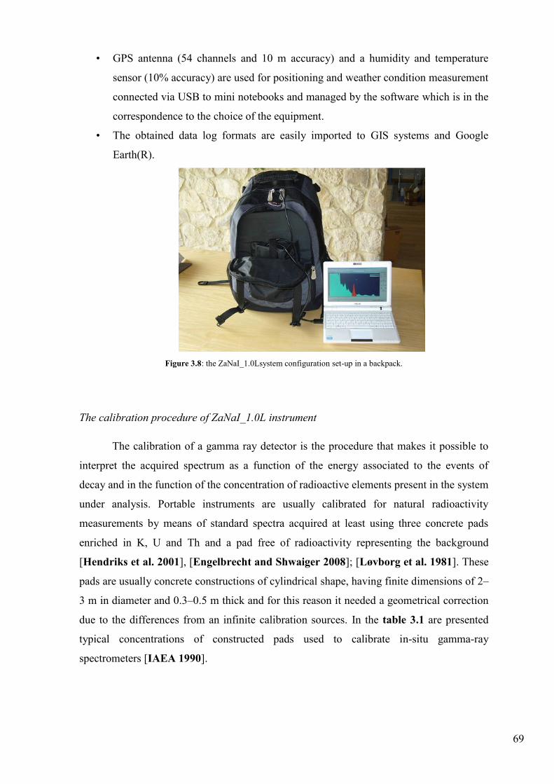
69
• GPS antenna (54 channels and 10 m accuracy) and a humidity and temperature
sensor (10% accuracy) are used for positioning and weather condition measurement
connected via USB to mini notebooks and managed by the software which is in the
correspondence to the choice of the equipment.
• The obtained data log formats are easily imported to GIS systems and Google
Earth(R).
Figure 3.8: the ZaNaI_1.0Lsystem configuration set-up in a backpack.
The calibration procedure of ZaNaI_1.0L instrument
The calibration of a gamma ray detector is the procedure that makes it possible to
interpret the acquired spectrum as a function of the energy associated to the events of
decay and in the function of the concentration of radioactive elements present in the system
under analysis. Portable instruments are usually calibrated for natural radioactivity
measurements by means of standard spectra acquired at least using three concrete pads
enriched in K, U and Th and a pad free of radioactivity representing the background
[Hendriks et al. 2001], [Engelbrecht and Shwaiger 2008]; [Løvborg et al. 1981]. These
pads are usually concrete constructions of cylindrical shape, having finite dimensions of 2–
3 m in diameter and 0.3–0.5 m thick and for this reason it needed a geometrical correction
due to the differences from an infinite calibration sources. In the table 3.1 are presented
typical concentrations of constructed pads used to calibrate in-situ gamma-ray
spectrometers [IAEA 1990].

70
Table 3.1: typical concentrations of constructed pads used to calibrate in-situ gamma-ray spectrometers (IAEA 1990).
The design of an ideal pad with one radionuclide inside and with a perfect homogeneous
distribution of the radioisotope in its volume is impossible, because impurities and non-
homogeneities are always present. For this reason, compromises between accuracy and
applicability of the method have to be weighted.
Generally the Window Analysis Method (WAM) is applied as spectrum analysis
method to assess the concentration of potassium by studying the single peak emitted from
40K to an energy of 1460 keV, of uranium
238U through the detection of gamma rays of
1765 keV from 214
Bi, while in the case of thorium 232
Th are studied gamma rays of 208
Tl
with energy equal to 2614 keV. The IAEA recommend the following energy windows in
order to evaluate the counts rate (Table 3.2).
Table 3.2: standard gamma ray energy windows recommended for natural radioelement mapping.
A generic site of calibration, it is obtained by evaluating the area under the spectrum within
the energy bands previously defined, the number of counts in the windows of potassium,
uranium and thorium, respectively NK, NU, NTh.

71
Figure 3.9: energy windows for the WAM analysis of a gamma spectrum.
The WAM method considers exclusively useful the signal associated to photopeaks
neglecting other spectral regions which, despite being less representative, also provide a
valuable complement to the analysis of the spectrum.
In our study, an alternative calibration procedure is used instead of building pads,
which is based on the selection of sites characterized by a prevalent concentration of one of
the natural radionuclides (Table 3.3). Since, the measurements in-situ can be affected by
the specificity of the place, like the soil non-homogeneity, the ground morphology, the
non-secular equilibrium in radioactive chains, the vertical distribution of 137
Cs, the
presence of vegetation, moisture, etc. the calibration sites should be selected according
precise prescriptions:
• relatively uniform distribution of radionuclides in secular equilibrium with their products,
• plane area without any steps and large enough to be approximated as an infinite source
(maximum 10 m radius) [Grasty et al 1975],
• undisturbed areas assuring relatively constant 137
Cs vertical distribution,
• uniform and relatively homogeneous soil moisture content and vegetable coverage,
The concentrations reported in table 3.3 are the average of the measurements
performed in the laboratory on the collected rock samples. This way the heterogeneity of
each site is properly implemented by the errors which are dominated by the spread in the
results of the collected samples in each calibration site.
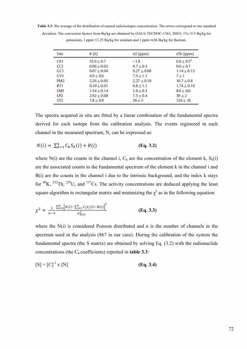
72
Table 3.3: the average of the distribution of natural radioisotopes concentration. The errors correspond to one standard
deviation. The conversion factors from Bq/kg are obtained by (IAEA-TECDOC-1363, 2003): 1%=313 Bq/kg for
potassium, 1 ppm=13.25 Bq/kg for uranium and 1 ppm=4.06 Bq/kg for thorium.
The spectra acquired in situ are fitted by a linear combination of the fundamental spectra
derived for each isotope from the calibration analysis. The events registered in each
channel in the measured spectrum, N, can be expressed as:
∑ (Eq. 3.2)
where N(i) are the counts in the channel i, Ck are the concentration of the element k, Sk(i)
are the associated counts to the fundamental spectrum of the element k in the channel i and
B(i) are the counts in the channel i due to the intrinsic background, and the index k stays
for 40
K, 232
Th, 238
U, and 137
Cs. The activity concentrations are deduced applying the least
square algorithm to rectangular matrix and minimizing the χ2 as in the following equation:
∑ [ ∑ ]
(Eq. 3.3)
where the N(i) is considered Poisson distributed and n is the number of channels in the
spectrum used in the analysis (867 in our case). During the calibration of the system the
fundamental spectra (the S matrix) are obtained by solving Eq. (3.2) with the radionuclide
concentrations (the Ck coefficients) reported in table 3.3:
[S] = [C]-1
x [N] (Eq. 3.4)

73
Figure 3.10: the sensitive spectra obtained through the FSA with NNLS constraint.
3.3 In-situ spectrum acquisition
Each point at which were performed the in-situ measurements, are chosen in such
way to be as flat as possible and preferably at least 20 meters away from roads and man-
made structures of large dimensions (houses, boundary walls, bridges, etc..). The latter
arrangement is necessary in order to avoid interference during acquisition. The distance of
20 m is cautionary since, as shown in figure 3.7, 90% of the signal is received from an
area of 7.35 m radius. First, in the selected site is made an acquisition to perform the
energetic calibration of the instrument in order to be able to relate the acquisition channel
with the energy associated with it. It is recognized the photopeak of the potassium and the
channel having the largest number of counts is assigned an energy equal to 1.460 MeV. If
the calibration of energy has been carried out correctly even relative peaks of uranium and
thorium fall inside its windows having energy values reported above in table 3.2.
Once completed the preliminary phase of instrument calibration, will proceed with
the acquisition of the spectra. During the campaign activity in Ombrone basin and Schio
Commune were acquired a total of 338 spectra. In particular, in order to study the
influence of acquisition parameter were acquired:

74
in Ombrone basin:
- 80 spectra by placing the ZaNaI_1.0L on the ground (Figure 3.11) in
correspondence with 400 soil samples collected in order to characterize the site (see
below);
- 80 spectra by placing the ZaNaI_1.0L a tripod at 1m height (Figure 3.12) in
correspondence with 400 soil samples collected in order to characterize the site (see
below);
- 80 spectra by placing the ZaNaI_1.0L on a tripod at 1m height (Figure 3.12) in
correspondence with 80 spectra by placing the ZaNaI_1.0L on the ground (Figure
3.11);
in Schio Commune:
- 89 spectra by placing the ZaNaI_1.0L on the shoulders of an operator (Figure 3.13)
in correspondence with 89 spectra by placing the ZaNaI_1.0L on the ground
(Figure 3.11).
Each acquisition had duration of 5 minutes.
Figure 3.11: example of acquisition of the spectrum with backpack placed on the ground.

75
Figure 3.12: example of acquisition of the spectrum with backpack placed on the tripod at 1 m height above the
ground.
Figure 3.13: example of acquisition of the spectrum with backpack placed on the shoulders.

76
3.4 Soil sampling
The measurement in situ with portable instrumentation is strongly influenced by the
surrounding environment and is fundamental the knowledge of the main environmental
parameters and the characteristics of terrain. For this, in each chosen site was performed a
measurement of radioactivity with the instrument ZaNaI_1.0L also have been taken five
different soil samples to be subsequently analyzed in the laboratory. The samples were
collected following a provision to "star": a central sample is extracted at the point in which
it was positioned backpack and the four samples at a distance of about one meter (Figure
3.14). The soil is collected with a trowel to a maximum depth of 10 cm, avoiding to take
roots, leaves or materials not representative of the soil itself. The amount removed is never
less than 500 g. The bag is closed with adhesive tape and on the bag is shown the ID
(Soil_X, where X is a progressive number) sample identification. In total 80 different sites
were analyzed and were collected 400 samples of soil. All operations are documented by
photos.
Figure 3.14: example of the soil samples arrangement with respect to the central point in which is realized the
measurement of gamma-ray spectroscopy in situ.
For a better characterization of the environment in which it was carried out a
measurement of natural radioactivity, in addition to recording the coordinates with the GPS
antenna are measured some environmental parameters (temperature and humidity) and
describes the pedological and geological characteristics of the soil in site. In fact there is a
measurement procedure for soils which consists of the compilation in campaign of

77
geodatabase Rad_Nat.mdb in which are inserted the necessary characteristic parameters for
the characterization of the soil sample. The environmental parameters and pedological to
be defined in the campaign are reported in table 3.4 and table 3.5.
Table 3.4: standard pedological parameters to define in the campaign.
Pedology parameters Description
Lithology
Both chemical and physical
characteristics that define a rock in its
various aspects, namely chemical and
mineralogical composition, structure and
texture.
Rockiness Information indicating the content of
rockiness in the surrounding area.
Use of soil
Use of soil is all that pertains to the use
and management strategies of certain land
cover by man.
PH of soil Parameter that identifies the acidity of
soil.
Colour
It is an important feature as it can be
indicator of genetic variations and
behavior.
Presence of mottles
Recognition of chromatic variations with
respect to the predominant color of the
terrigenous matrix.
Water content
Provides an indication of the amount of
present water: according to the condition
of the soil (dry, wet or saturated) varies
the consistency at the same.

78
Table 3.5: environmental parameters monitored during the in situ measurement.
Environmental
Parameters Description Instrumention
Configuration of
acquisition
This parameter takes into account the
geometry of the environment in which the
measurement is carried out
NaI(Tl)
Humidity
Important parameter for the definition of
the environmental conditions of
measurement.
Humidity sensor
Temperature
Important parameter for the definition of
the environmental conditions of
measurement
Temperature sensor
Climatic condition
Useful data for the definition of the
environmental conditions of
measurement, which vary in the presence
or absence of precipitation meteorological
Detector campaign
Density of
vegetative cover
Indicative information for both the in situ
measurement and for the soil sampling Detector campaign
Tipology of
vegetative cover
Information of interest for a more detailed
analysis of the environment, both for the
in situ measurement and for the soil
sample
Detector campaign
Number of soil
sampling
Necessary parameter for ascending to the
environmental conditions of measurement Detector campaign
Measurement
distance from the
sampling point in
the soil
Important parameter to be used for the
study of the environmental conditions Detector campaign
Spatial coordinates
of the acquisition
point
Information fundamental to be able to
ascend the point of sampling and
measuring
GPS 54 channels

79
Chapter 4
4. Laboratory activity
This chapter will describe the procedure for the preparation of soil samples to be
analyzed with the MCA_Rad system.
4.1 Preparation of samples
Each of 400 samples was crushed, homogenized (in less than 2 mm fine grain size)
and constant weight dried at 110°C temperature (Figure 4.1). Then, the samples were
sealed in cylindrical polyethylene plastic containers (7.5 cm of diameter and 4.5 cm height)
of 180 cm3 effective volume. The soil samples were subsequently labeled with ID of the
sample and after that were weighed. After, each sealed container is left undisturbed for at
least four weeks before spectrum acquisition in order to establish the equilibrium between
226Ra and its short lived progenies (
222Rn).
Figure 4.1: ventilated oven used to dry the soil samples.
Each box is also assigned a bar code (Figure 4.2), necessary for their automatic
identification. All data obtained from this procedure are stored in the Rad_Nat.mdb
geodatabase. The material not used is kept sealed in the original plastic bags.

80
Figure 4.2: soil samples ready to be analyzed with MCA_Rad system.
4.2 High resolution gamma-ray spectrometry using the MCA_Rad system
The MCA_Rad system (Figure 4.3) introduces an innovative configuration of a
laboratory high-resolution gamma-ray spectrometer featured with a complete automation
measurement process, which can conduct measurements on each type of material (solid,
liquid or gaseous) in less than 1 hour.
The activity concentrations of 40
K, 238
U and 232
Th were measured by using the
MCA_Rad system, described in details in [Xhixha, G., et, al, 2012]. The MCA_Rad
system is made of two 60 % relative efficiency coaxial p-type HPGe gamma-ray detectors,
which possess an energy resolution of about 1.9 keV at 1332.5 keV (60
Co). The detectors
are accurately shielded and positioned facing each other 5 cm apart. Both detectors are
controlled by individual integrated gamma spectrometers for the digital signal processing.
A new mechanical coolers, allows to simplify the management of the system. In table 4.1
the features of two detectors used for design of MCA_Rad system are presented.

81
Figure 4.3: MCA_Rad system composed by two coupled HPGe detectors.
Table 4.1: the features of two detectors used for design of MCA_Rad system (these values are measured by the
manufacturer).
Thanks to a shielding construction of lead with dimensions 20 cm × 25 cm × 20 cm and
copper with dimensions 10 cm × 15 cm × 10 cm (Figure 4.4) is reached a background
reduction of two order of magnitude with respect to laboratory radioactivity (Figure 4.5).

82
Figure 4.4: MCA_Rad system shielding of HPGe detectors composed by copper and lead.
Figure 4.5: MCA_Rad system background spectra (live time 100 h) without (red) and with (green) shielding showing a
reduction of two order of magnitudes.
The calibration of absolute full energy peak efficiency was determined through
certified standard point sources (152
Eu and 56
Co). The absolute efficiency calibration is
validated through the measurement of certified reference materials RGK_1, RGU_1 and
RGTh_1 [IAEA, 1987], showing an overall uncertainty to be then 5%. The absolute
efficiency of the standard point source εp (E) in the energetic range from 200 to 3000 keV
is obtained by fitting the function described by Knoll 1999 (Figure 4.6).

83
Figure 4.6: absolute efficiency curve for the MCA_Rad system obtained by fitting the corrected values for coincidence
summing with equation 2.16. Apparent efficiencies of 152Eu (blue triangles) and 56Co (green squares) are also presented.
(
)
(
) (
) (Eq. 4.1)
where E is the energy of gamma ray and E0 is introduced to make the argument of the
logarithm dimensionless. The correction due to coincidence summing is studied by
following the method described in [De Felice P., et, al, 2000] and obtained as a
relationship between the single total efficiency (εt), the single apparent absolute photopeak
efficiency (εapp) and isotope decay data.
The spectra obtained are corrected for: (1) differences between the geometry of the
point sources and the sample shape, CG and (2) self-attenuation, CSA, of gamma-rays
within the sample volume.
The geometrical factor for MCA_Rad system is deduced from a set of
measurements using 56
Co and 57
Co point sources placed at different radial distances from
the detector axis on three different planes.
∑[ ]
(Eq. 4.2)

84
where Rx (Ei) is the net count rate in the standard spectrum collected in different positions
(j) and Rref (Ei) is the net count rate in the standard spectrum collected in the reference
positions (center). The geometrical correction factor was then fitted as a function of energy
and considered independently in order correct the efficiency curve of the standard point
source.
∑ (
)
(Eq. 4.3)
where n = 4 and ai are the fitting coefficients (a1 = 0.8678, a2 = 0.1098, a3 = -0.0541, a4 =
0.0077).
The self-absorption correction factor was calculated following a simple approach
discussed by Bolivar et al. 1997 and Cutshall et al. 1983:
( )
( ) (Eq. 4.4)
where are the densities of test sample and reference material,
are the densities of sample and reference material and t is the sample thickness.
The self-attenuation correction factor was then given as a function of energy and
considered independently in order correct the efficiency curve of the standard point source.
[ ] (Eq. 4.5)
The soil samples, contained in cylindrical containers of polycarbonate, are placed
on a loader tilted (Figure 4.7) at the end of which is positioned a reader of bar code and a
piston which introduces the sample into the measuring chamber, between the two faces of
the detector, through an opening rectangular of 5 × 10 cm2. A fully automation system
enables up to 24 samples to be measured without any human attendance. An acquisition
unit multichannel data managed by software developed in the Windows ambient controls
the procedures of measuremen and the change of the sample. The electronics associated
with the detector and measurement of gamma-ray spectroscopy is managed by the Maestro
software installed on the PC that controls the entire MCA_Rad system.

85
Figure 4.7: loader of samples and instrumentation for reading the bar code of MCA_Rad system.
The activity concentration of 40
K was determined from gamma energy emissions at
1460 keV. While the specific activity concentrations of 238
U and 232
Th were instead
determined, assuming the secular equilibrium in their respective decay chains, from
gamma energy emissions at 609 keV (214
Bi), 351.9 keV (214
Pb) for 238
U and 911.2 keV
(228
Ac), 238.6 keV (212
Pb), 583.2 keV (208
Tl) for 232
Th. Samples were firstly measured for
1 hour typical counting time, and repeating the measurements for longer acquisition times
until statistical errors become less than 20% (when reasonably possible).
The specific activity calculated using the formula:
A (Bq/kg) =
(Eq. 4.6)
where R is the measured count rate (background corrected), ε is the absolute efficiency,
is the gamma line intensity, m is the mass of the sample, CSA is the correction factors for
self-absorption, CG is the geometrical correction factor and is the coincidence summing
correction factor.

86
Chapter 5
5. Discussion of obtained results
In the first part of this chapter will be discussed briefly the methodology used for
the analysis of spectra. In the second one the analysis of the obtained results in particular
has focused on the study of four different types of correlation: correlation between in-situ
acquisition on ground and laboratory measurements, correlation between in-situ acquisition
on tripod and laboratory measurements, correlation between in-situ acquisition on ground
and on tripod and correlation between in-situ acquisition on ground and on operator
shoulder.
5.1 Spectrum analysis
A spectrum gamma acquired in natural environment is mainly composed by a
photopeak associated with the decay of 40
K, more than a dozen of emission photopeaks
associated with the decay of 238
U, and a similar number of photopeaks for the 232
Th.
However only some of them are distinguishable and well-formed above the spectrum of
background, and are based on the principle that identifies the photopeaks relatively to
which make a count of events.
As described above the Full Spectrum Analysis (FSA) reconstruct the measured
spectrum composing linearly the entire fundamental spectra of potassium, uranium and
thorium. The FSA method therefore uses all counts corresponding to the energy range from
300 to 2900 keV and not only those obtained in the standard energy windows (Figure 5.1).

87
Figure 5.1: representation of the total measured spectrum obtained by the superposition of the fundamental
spectra of cesium, potassium, uranium and thorium, and the background spectrum.
Therefore with this method determines the shape of the spectrum from the superimposition
of the different spectral components (Figure 5.1). The weight of each component is given
from the isotopic abundance, that as a result of a chi-square minimization process (Eq.
3.3).
[C] = [S]-1
[N] (Eq. 5.1)
5.2 Soil sample data: statistical analysis
From the analysis of the spectra are obtained the rate of net counts for the 40
K,
238U and
232Th. Taking into account the density of the sample, self-absorption and
efficiency of the system, are obtained the specific activities in Bq/kg. By using the
conversion factors given in table 5.1 are obtained the abundances of K (%), eU (ppm) and
eTh (ppm).
Table 5.1: conversion factors between specific activity and concentrations of K, eU and eTh3.
3 Guidelines for radioelement mapping using gamma ray spectrometry data. IAEA-TECDOC-1363, 2003.

88
All measured parameters and spectra obtained during this procedure are recorded in the
Rad_Nat.mdb. geodatabase.
It should be noted that there are various factors that influence the precision of the
analysis; in particular, in addition to the intrinsic radioactivity of the detector and the
presence of cosmic rays, must be taken into account the statistical nature of the decay
process (therefore related to the acquisition time), the variability of the radiation due to
atmospheric radon, the environmental characteristics, and the geometry of the source.
In order to carry out a study on the correlation between measures of environmental
radioactivity and radioactivity measurements in soil samples must have the same number
of parameters to compare. It is therefore necessary to obtain a single value of the
abundances of 40
K, 238
U and 232
Th for each group of five samples of soil belonging to the
same site. In many geological and environmental situations, the data distributions tend to
be positively asymmetric.
Often, if it is proceed the logarithms of the original values, where is obtained a
series of normally distributed data. If the variable X, has log-normal distribution, the
variable Y has a normal distribution such that:
(Eq. 5.2)
The density function of the lognormal variable X is defined by the following equation:
√
, X > 0 (Eq. 5.4)
where µ and σ is the median of the distribution of the logarithms of the X values and the σ
is their standard deviation. If the mean, median and variance of X are denoted respectively
by , and σ2 the relationships between the parameters expressed in the original scale and in
that logarithmic one are summarized in table 5.2.
Table 5.2: relationships between the parameters of the distribution in the original scale and in that logarithmic one.
Parameters Log-normal distribution
Mode
Mean
Variance
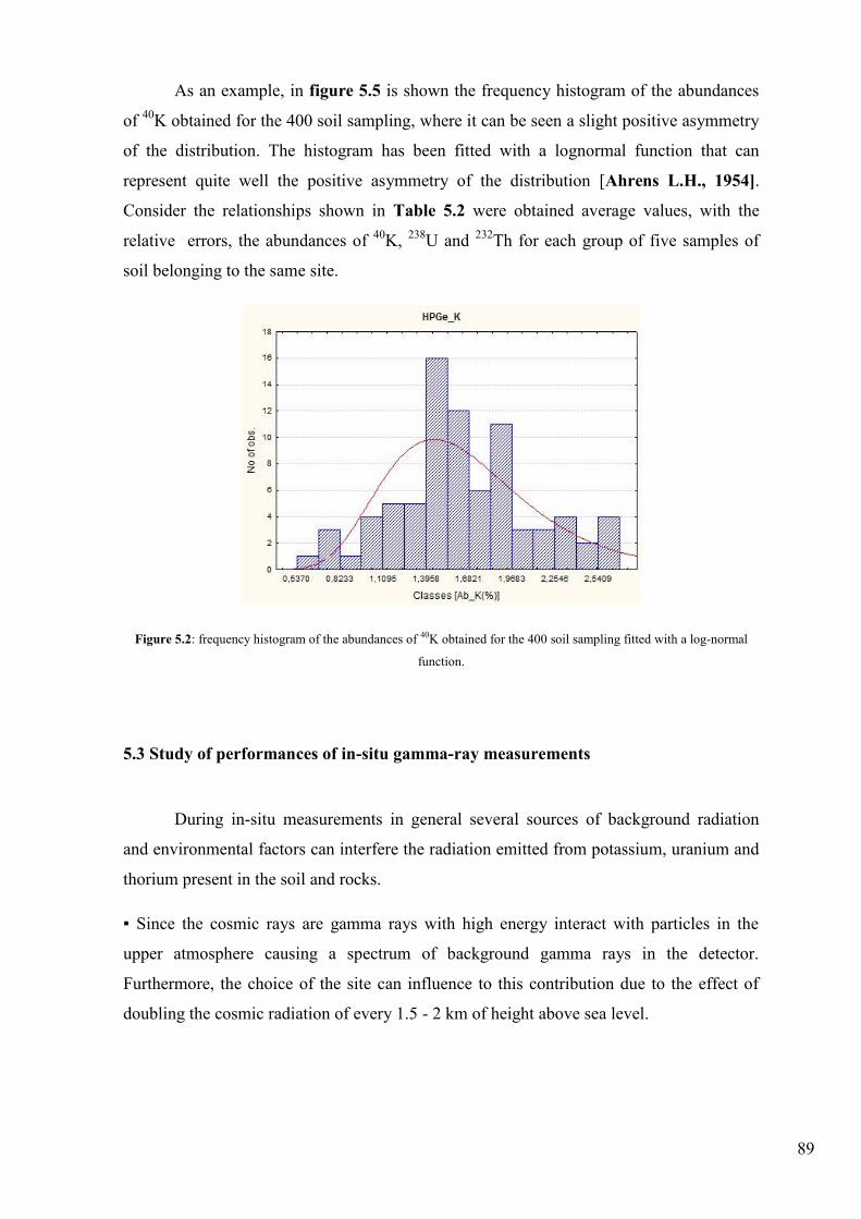
89
As an example, in figure 5.5 is shown the frequency histogram of the abundances
of 40
K obtained for the 400 soil sampling, where it can be seen a slight positive asymmetry
of the distribution. The histogram has been fitted with a lognormal function that can
represent quite well the positive asymmetry of the distribution [Ahrens L.H., 1954].
Consider the relationships shown in Table 5.2 were obtained average values, with the
relative errors, the abundances of 40
K, 238
U and 232
Th for each group of five samples of
soil belonging to the same site.
Figure 5.2: frequency histogram of the abundances of 40K obtained for the 400 soil sampling fitted with a log-normal
function.
5.3 Study of performances of in-situ gamma-ray measurements
During in-situ measurements in general several sources of background radiation
and environmental factors can interfere the radiation emitted from potassium, uranium and
thorium present in the soil and rocks.
▪ Since the cosmic rays are gamma rays with high energy interact with particles in the
upper atmosphere causing a spectrum of background gamma rays in the detector.
Furthermore, the choice of the site can influence to this contribution due to the effect of
doubling the cosmic radiation of every 1.5 - 2 km of height above sea level.

90
▪ The atmospheric radon (222
Rn) gas, can cause significant interference in the uranium
signal, particularly when atmospheric inversion traps them close to the ground [Darnley
and Grasty, 1970], [Grasty, 1979b].
▪ Rain and soil moisture increases the attenuation of gamma rays and cause the fluence
rate of potassium and thorium to be decreased, generally by 10% for every 10% increase in
soil moisture [Kogan et al., 1969]. In the case of uranium the effect is more complicated
because radon escapes more readily from drier soils [Megumi and Mamuro, 1973]. In
wetter soils the lower escape rate can result in a build-up of radon in the near surface and
an apparent increase in uranium content [Tanner, 1964], [Lovborg, 1984]; [Grasty,
1997]. Also during rainfall the uranium signal can increase rapidly, due to daughter
products of radon disintegration, attach to airborne aerosols and dust and can precipitate
with the rain drops [Charbonneau and Darnley, 1970].
▪ The vegetative cover, having dense composition, can cause some shielding of radiation
and may also contribute to the gamma ray flux through radioisotopes within the biomass.
Evident is in the forested areas, tree trunks can collimate the flux of gamma rays [Kogan
et al., 1969], [Travassos and Pires, 1994].
In this study we have neglected the cosmic radiation variation since the sites are
chosen at similar heights above sea-level. The effect of rainfall on soil moisture and
gamma-ray attenuation is also neglected since all in-situ measurements are performed
always at least 1 week after rainfalls. Instead the radon influences on uranium signal it is
discussed in our results together with the attenuation effect of vegetative cover.
In particular, we have studied the performances of in-situ measurements by
studying the correlation between in-situ measurements on-ground/tripod and laboratory
measurements on sample. Furthermore we have studied the effect of the morphology of the
site and the attenuation factor of 1 m air by observing the correlation between in-situ
measurements obtained by placing the ZaNaI_1.0L on ground and on tripod. Also the
attenuation effect of the presence of the operator during in-situ measurements obtained by
placing the detector on-shoulder was studied.

91
5.3.1 Correlation between in-situ acquisition on ground and laboratory measurements
For studying the correlation between the measurements of environmental
radioactivity measured in situ with the instrument ZaNaI_1.0L and the results obtained
from the analysis of soil samples, has been compared the relative abundances of 40
K, 238
U
and 232
Th obtained by MCA_Rad system with those obtained by ZaNaI_1.0L on the
ground (Table 5.3). For each distribution was calculated the weighted linear regression for
errors using a MATLAB code by imposing its passage through the origin of the coordinate
system.
Figure 5.3: the correlation between the abundance of K measured on sample using HPGe detectors and the
abundance of K measured in-situ using ZaNaI_1.0L placed on the ground is described by the relationship
KZaNaI = (1.16 ± 0.05) KHPGe with r2 = 0.90.

92
Figure 5.4: the correlation between the abundance of eU measured on sample using HPGe detectors and the
abundance of eU measured in-situ using ZaNaI_1.0L placed on the ground is described by the relationship
eUZaNaI = (0.85 ± 0.11) eUHPGe with r2 = 0.64.
Figure 5.5: the correlation between the abundance of eTh measured on sample using HPGe detectors and the
abundance of eTh measured in-situ using ZaNaI_1.0L placed on the ground is described by the relationship
eThZaNaI = (0.97 ± 0.12) eThHPGe with r2 = 0.80.
The bar of errors relative to the values obtained with the MCA_Rad represents the
standard deviation of the log-normal distribution of the 5 samples related to the measured
site. The error bar relative to the values obtained with the ZaNaI_1.0L is the instrumental
error. In table 5.3 are summarized the parameters of correlation between in-situ and
laboratory measurements.

93
Table 5.3: the correlation parameters obtained for in-situ measurements on ground and laboratory measurements.
Isotopes a ± σa r2
K [%] 1.16 ± 0.05 0.90
U [mg/Kg] 0.85 ± 0.11 0.64
Th [mg/Kg] 0.97 ± 0.12 0.80
From these results it can be seen that there is good correlation between in-situ and
laboratory measurements. In particular, the linear regression coefficient r2 obtained for K
and Th is very close to unity. While, the linear regression coefficient obtained for U show a
relatively good correlation when as it can be expected the data are more dispersed due to
the effect of atmospheric radon (no correction for atmospheric radon are applied to in-situ
measurements). For Th the data are comparable within 1σ, while for U within 1.5σ and for
K for more than 3σ. However, the final relative uncertainties for K, U and Th are less than
about 20%, respectively 13%, 19% and 12%.
5.3.2 Correlation between in-situ acquisition on tripod and laboratory measurements
The previous study was repeated by comparing in-situ measurements using
ZaNaI_1.0L placed on tripod and the results obtained from soil sample measurements
using the MCA_Rad system.

94
Figure 5.6: the correlation between the abundance of K measured on sample using HPGe detectors and the
abundance of K measured in-situ using ZaNaI_1.0L placed on the tripod is described by the relationship
KZaNaI = (1.11 ± 0.05) KHPGe with r2 = 0.88.
Figure 5.7: the correlation between the abundance of eU measured on sample using HPGe detectors and the
abundance of eU measured in-situ using ZaNaI_1.0L placed on the tripod is described by the relationship
eUZaNaI = (0.75 ± 0.10) eUHPGe with r2 = 0.66.

95
Figure 5.8: the correlation between the abundance of eTh measured on sample using HPGe detectors and the
abundance of eTh measured in-situ using ZaNaI_1.0L placed on the tripod is described by the relationship
eThZaNaI = (0.92 ± 0.11) eThHPGe with r2 = 0.79.
In table 5.4 are summarized the parameters of correlation between in-situ and
laboratory measurements.
Table 5.4: correlation between measurements in-situ acquisition on tripod and in the laboratory.
Isotopes a ± σa r2
K [%] 1.11 ± 0.05 0.88
U [mg/Kg] 0.75 ± 0.10 0.66
Th [mg/Kg] 0.92 ± 0.11 0.79
From these results it can be seen that there is good correlation between in-situ and
laboratory measurements. The linear regression coefficient shows similar results as those
obtained for in-situ measurements placing the detector on ground. For Th the data are
comparable within 1σ, while for U within 2.5σ and for K for more than 2σ. However, the
final relative uncertainties for K, U and Th are less than about 35%, respectively 10%, 33%
and 12%. The increase of discrepancy between the two data sets can be attributed to the
attenuation of 1m air for in-situ measurement performed by placing the detector on tripod.

96
The attenuation due to 1 m air can be calculated as the difference between ground and
tripod in-situ measurements compared with laboratory measurements, and are 5 ± 0.3 %,
10 ± 1.9 % and 5 ± 0.9 % respectively for K, U and Th.
5.3.3 Correlation between in-situ acquisition on ground and on tripod
To quantify the correction of signal mainly caused by the presence of about 1 m air
between the detector and the source (earth surface) is done also by comparing in-situ
measurements obtained by placing the ZaNaI_1.0L on ground and on tripod. The definition
of these correction, allows to refer the measured abundances of 40
K, 238
U and 232
Th to soil
concentration In addition, also the analysis of 137
Cs was included.
Figure 5.9: the correlation between the abundance of K measured by placing the ZaNaI_1.0L on ground and on
tripod is described by the relationship Kground= (0.93 ± 0.03) Ktripod with r2 = 0.98.

97
Figure 5.10: the correlation between the abundance of eU measured by placing the ZaNaI_1.0L on ground and
on tripod is described by the relationship eUground= (0.87 ± 0.03) eUtripod + (0.31 ± 0.14) with r2 = 0.73.
Figure 5.11: the correlation between the abundance of eTh measured by placing the ZaNaI_1.0L on ground and
on tripod is described by the relationship eThground= (0.94 ± 0.06) eThtripod with r2 = 0.96.

98
Figure 5.12: the correlation between the abundance of 137Cs measured by placing the ZaNaI_1.0L on ground
and on tripod is described by the relationship 137Csground= (0.81 ± 0.02) 137Cstripod with r2 = 0.95.
The bar of the errors relative to the obtained abundances with the ZaNaI_1.0L both on
ground and the height 1 m represents the instrumental error, and thus results to be the same
for both measurements.
In table 5.5 are summarized the parameters of correlation between in-situ and
laboratory measurements.
Table 5.5: correlation parameters between in-situ measurements on ground and on tripod.
Isotopes a ± σa b ± σb r2
K [%] 0.93 ± 0.03 - 0.98
U [mg/Kg] 0.87 ± 0.06 0.31 ± 0.14 0.73
Th [mg/Kg] 0.94 ± 0.06 - 0.96
137Cs [cps] 0.81 ± 0.02 - 0.95
From these results it can be seen that there is very good correlation between in-situ
measurements. Since the detector at 1 m height receives the signal from a bigger area with
respect to the same positioned on the ground (Figure 3.5, Figure 3.6, and Figure 3.7), the
close to unity linear regression coefficient are an evidence of the homogeneity of the

99
selected sites. The deviation between the angular coefficients and the unity value quantifies
the correction of the signal due to the attenuation effect of 1 m air, obtaining for 40
K, 238
U,
232Th and
137Cs respectively 7 ± 0.3%, 13 ± 0.9 %, 6 ± 0.4% and 19 ± 0.5%. Compared
with the results described in section 5.3.2 the results are comparable within 1σ for Th and
U while more than 3σ away for K. For 137
Cs the attenuation is higher due to the fact that it
emits a gamma ray with relative lower energy (662 keV).
5.3.4 Correlation between in-situ acquisition on ground and on operator shoulder
During dynamic spectrum acquisition, by holding the detector on the operator shoulders, it
is important to evaluate the interference of the operator. For this reason, a comparison
between the abundances obtained with the ZaNaI_1.0L placed on the ground and held in
the shoulder of an operator is performed.
Figure 5.13: the correlation between the abundance of K measured by placing the ZaNaI_1.0L on ground and
on shoulder is described by the relationship Kground= (0.82 ± 0.01) Kshoulder + (0.08 ± 0.01) with r2 = 0.97.

100
Figure 5.14: the correlation between the abundance of eU measured by placing the ZaNaI_1.0L on ground and
on shoulder is described by the relationship eUground= (0.84 ± 0.01) eUshoulder + (0.13 ± 0.03) with r2 = 0.98.
Figure 5.15: the correlation between the abundance of eTh measured by placing the ZaNaI_1.0L on ground and
on shoulder is described by the relationship eThground= (0.83 ± 0.02) eThshoulder with r2 = 0.97.

101
Figure 5.16: the correlation between the abundance of 137Cs measured by placing the ZaNaI_1.0L on ground
and on shoulder is described by the relationship 137Csground= (0.77 ± 0.01) 137Csshoulder with r2 = 0.95.
In table 5.6 are summarized the parameters of correlation between in-situ and
laboratory measurements.
Table 5.6: correlation parameters between in-situ measurements on ground and on shoulder.
Isotopes a ± σa b ± σb r2
K [%] 0.82 ± 0.01 0.08 ± 0.01 0.97
U [mg/Kg] 0.84 ± 0.01 0.13 ± 0.03 0.98
Th [mg/Kg] 0.83 ± 0.02 - 0.97
137Cs (cps) 0.77 ± 0.01 - 0.95
From these results it can be seen that there is very good correlation between in-situ
measurements. The deviation between the angular coefficients and the unity value
quantifies the correction of the signal due to the presence of an operator, obtaining for 40
K,
238U,
232Th and
137Cs respectively 18 ± 0.2%, 16 ± 0.2 %, 17 ± 0.4% and 23 ± 0.3%.

102
5.3.5 Interference of vegetative cover for-situ acquisition on ground and on operator
shoulder
During the in-situ measurements may by differences between sites due to the
presence or not of the vegetative cover. We make and attempt to evaluate such a presence
by classifying the sites into two classes of vegetative coverage from 0-50% and 50-100%.
Therefore, we compared the results obtained by in-situ measurements by placing the
detector on ground and holding it on shoulders. In the case of 40
K and 238
U this influence is
found to be negligible within the reported uncertainty, while for 232
Th and 137
Cs it is
observed a slight interference due to the presence of the vegetative cover.
Figure 5.17: for 0-50% vegetative cover case: the correlation between the abundance of Th measured by
placing the ZaNaI_1.0L on ground and on shoulder is described by the relationship
Thground= (0.83 ± 0.02) Thshoulder with r2 = 0.99.
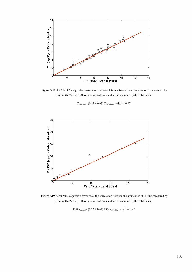
103
Figure 5.18: for 50-100% vegetative cover case: the correlation between the abundance of Th measured by
placing the ZaNaI_1.0L on ground and on shoulder is described by the relationship
Thground= (0.85 ± 0.02) Thshoulder with r2 = 0.97.
Figure 5.19: for 0-50% vegetative cover case: the correlation between the abundance of 137Cs measured by
placing the ZaNaI_1.0L on ground and on shoulder is described by the relationship
137Csground= (0.72 ± 0.02) 137Csshoulder with r2 = 0.97.

104
Figure 5.20: for 50-100% vegetative cover case: the correlation between the abundance of 137Cs measured by
placing the ZaNaI_1.0L on ground and on shoulder is described by the relationship
137Csground= (0.77 ± 0.01) 137Csshoulder with r2 = 0.96.
In table 5.7 are summarized the parameters of correlation between in-situ and
laboratory measurements.
Table 5.7: correlation parameters between in-situ measurements on ground and on shoulder for two classes of
vegetative coverage.
Isotopes a ± σa
Vegetative coverage 0-50 %
Vegetative coverage 50-100 %
Th [mg/Kg] 0.83 ± 0.02 0.85 ± 0.02
137 Cs [cps] 0.72 ± 0.02 0.77 ± 0.01
In the case of 232
Th it is observed a minor degree of influence due to the vegetative cover
from 50-100%, but comparable within 1σ with the case of 0-50% of vegetative coverage.
While, in the case of 137
Cs it is seen clearly within the 1σ the influence due to the presence
of the vegetative cover. As it is expected, the presence of vegetative cover is more visible
in the case of relatively lower energies.

105
Chapter 6
6. Conclusions
In this work, have been studied several performances of portable detector
(ZaNaI_1.0L) composed by a solid scintillator NaI (Tl) of 1L of volume, designed and
built specifically to measure the radioactivity content in soils and rocks for geological and
environmental purposes. The aim of this thesis is the study of the performances of
measurements carried out in-situ with the ZaNaI_1.0L by comparing them with
measurements of the radioactivity content carried out in the laboratory on the soil samples
representative of the same area investigated by the portable detector. Furthermore, since
the ZaNaI_1.0L was designed to be used both in static and dynamic acquisition mode we
have studied the performances of the measurements performed in different situations.
The area in which were chosen the sites in which are made the measurements of
radioactivity is Ombrone basin, located in southern Tuscany and the Commune of Schio
located in the Region of Veneto. During the campaign activity were investigated 80 and 89
sites respectively in Ombrone basin and Schio district with a total of 338 spectra. In
addition, in each of the 80 sites investigated in Ombrone basin other than realizing a
measurement of radioactivity with the ZaNaI_1.0L, were taken 5 different soil samples,
with a total of 400 samples. The spectra acquired with ZaNaI_1.0L we analyzed using the
FSA-NNLS method in order to determine the abundances of 40
K, eU and eTh. Instead, the
soil samples were measured in the laboratory with a high-pure germanium detector
(MCA_Rad) and analyzed for 40
K, eU and eTh abundances.
In particular, we have studied the correlation between:
• 80 spectra by placing the ZaNaI_1.0L on the ground in correspondence with 400
soil samples collected in order to characterize the site;
• 80 spectra by placing the ZaNaI_1.0L a tripod at 1m height in correspondence with
400 soil samples collected in order to characterize the site;
• 80 spectra by placing the ZaNaI_1.0L on a tripod at 1m height in correspondence
with 80 spectra by placing the ZaNaI_1.0L on the ground;

106
• 89 spectra by placing the ZaNaI_1.0L on the shoulders of an operator in
correspondence with 89 spectra by placing the ZaNaI_1.0L on the ground.
In general several sources of background radiation and environmental factors as:
cosmic rays, atmospheric radon (222
Rn), rain and soil moisture, also the vegetative cover,
can interfere the radiation emitted from potassium, uranium and thorium present in the soil
and rocks during the measurements in-situ. In this study the influence due to changes on
cosmic radiation are considered negligible since the sites are chosen at similar heights
above sea-level. The effect of attenuation of gamma-rays due to changes in soil moisture
after rainfalls is also considered negligible since all in-situ measurements are always
performed at least 1 week after rainfalls. While the interference due to atmospheric radon
for the signal coming from uranium it is discussed only qualitatively in our results. Finally,
the attenuation effect due to vegetative cover is discussed and from the data it was possible
to determine such interference only in the case of 137
Cs, for the other isotopes the effect
was found to be negligible within the uncertainty.
The comparison between in-situ measurements both on ground and on tripod (1m
height) versus laboratory measurements shows a good correlation among them (Table 6.1).
Table 6.1: correlation between ZaNaI_1.0L measurements obtained by placing the detector on ground and on
tripod respect to laboratory measurements.
Isotope [ZaNaI]ground = (a ± σa) [HPGe] [ZaNaI]tripod = (a ± σa) [HPGe]
40K (%) 1.16 ± 0.05 1.11 ± 0.05
eTh (µg/g) 0.85 ± 0.11 0.75 ± 0.10
eU (µg/g) 0.97 ± 0.12 0.92 ± 0.11
The final relative uncertainties for K, U and Th are found to be less than about 20% for
ZaNaI_1.0L on ground versus HPGe measurements and about 35 % ZaNaI_1.0L on tripod
versus HPGe measurements.

107
The determination of the attenuation of air during in-situ measurements performed
by placing the detector at 1m height (tripod) are important in order to report that the results
at ground concentration of the radioactivity. For this purpose, we obtained this correction
by studying the results in table 6.1 and by comparing directly in-situ measurement
performed by placing the detector on-ground and on tripod. The results are found to be
comparable within 1σ for U and eTh and out for more than 3σ for K. The results show a
clear energy dependence of attenuation factor which decreases with increasing of gamma
ray energies with exception of eU which seems to be influences by the presence of radon
gas in air.
Table 6.2: attenuation correction due to air for in-situ measurements at tripod (1m height).
Isotopes
Max. energy
[keV]
air attenuation correction
[%]
137Cs [cps] 662 19 ± 0.5
K [%] 1460 7 ± 0.3
U [mg/kg] 1674 13 ± 0.9
Th [mg/kg] 2615 6 ± 0.4
An important application of ZaNaI_1.0L is the utilization in dynamic mode of
acquisition, where the detector configured in a back-pack in held on shoulder of an
operator. In order to correct for the attenuation effect due to the presence of the operator
we have compared the results obtained in-situ by placing the detector on ground and
holding on shoulders (table 6.3). Again is can be observed the energy dependence of
attenuation factor which decreases with increasing of gamma ray energies again with
exception of eU which seems to be influences by the presence of radon gas in air.

108
Table 6.3: attenuation correction due to the presence of the operator during in-situ dynamics acquisition
Isotopes
Max. energy
[keV]
air + operator attenuation correction
[%]
137Cs [cps] 662 23 ± 0.3
K [%] 1460 18 ± 0.2
U [mg/kg] 1674 16 ± 0.2
Th [mg/kg] 2615 17 ± 0.4
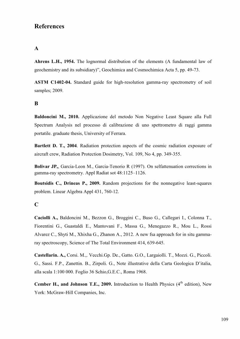
109
References
A
Ahrens L.H., 1954. The lognormal distribution of the elements (A fundamental law of
geochemistry and its subsidiary)”, Geochimica and Cosmochimica Acta 5, pp. 49-73.
ASTM C1402-04. Standard guide for high-resolution gamma-ray spectrometry of soil
samples; 2009.
B
Baldoncini M., 2010. Applicazione del metodo Non Negative Least Square alla Full
Spectrum Analysis nel processo di calibrazione di uno spettrometro di raggi gamma
portatile. graduate thesis, University of Ferrara.
Bartlett D. T., 2004. Radiation protection aspects of the cosmic radiation exposure of
aircraft crew, Radiation Protection Dosimetry, Vol. 109, No 4, pp. 349-355.
Bolivar JP,, Garcia-Leon M., Garcia-Tenorio R (1997). On selfattenuation corrections in
gamma-ray spectrometry. Appl Radiat sot 48:1125–1126.
Boutsidis C., Drineas P., 2009. Random projections for the nonnegative least-squares
problem. Linear Algebra Appl 431, 760-12.
C
Caciolli A., Baldoncini M., Bezzon G., Broggini C., Buso G., Callegari I., Colonna T.,
Fiorentini G., Guastaldi E., Mantovani F., Massa G., Menegazzo R., Mou L., Rossi
Alvarez C., Shyti M., Xhixha G., Zhanon A., 2012. A new fsa approach for in situ gamma-
ray spectroscopy, Science of The Total Environment 414, 639-645.
Castellarin. A., Corsi. M.,. Vecchi.Gp. De., Gatto. G.O., Largaiolli. T., Mozzi. G., Piccoli.
G., Sassi. F.P., Zanettin. B., Zirpoli. G., Note illustrative della Carta Geologica D’italia,
alla scala 1:100 000. Foglio 36 Schio,G.E.C., Roma 1968.
Cember H., and Johnson T.E., 2009. Introduction to Health Physics (4th
edition), New
York: McGraw-Hill Companies, Inc.

110
Charbonneau B. W., and Darnley A. G., 1970. Radioactive precipitation and its
significance to high sensitivity gamma-ray spectrometer surveys: Geological Survey of
Canada, Paper 70-1, B, 32-36.
Cutshall NH., Larsen IL., Olsen CR (1983). Direct analysis of Pb-210 in sediment
samples: self-absorption corrections. Nuclear Instrum Methods 206:309–312.
D
Darnley A. G. and Grasty R. L., 1970. Mapping from the air by gamma-ray
spectrometry: Proceedings Third International Symposium, Toronto, Can. Inst. Min. Met.
Spec., 11, 485-500. Darnley, A. G., Bristow, Q. and Donhoffer, D. K., 1968. Airborne
gamma-ray spectromet.
Das A., and Ferbel T., 2003. Introduction to Nuclear and Particle Physics (2nd edition),
London: World Scientific.
De Felice P., Angelini P., Fazio A., Biagini R (2000) Fast procedures for coincidence-
summing correction in gamma-ray spectrometry.Appl Radiat Isot 52:745–752.
Désesquelles P., Ha T.M.H., Korichi A., Le Blanc F., Petrache C.M., 2009. NNLC: non-
negative least chi-square minimization and application to HPGe detectors. J Phys G: Nucl
Part Phys 36, 037001–7.
E
Eisenbud M., and Gesell T., 1997. Environmental Radioactivity from Natural Industrial,
and Military Sources (4th edition), London: Academic Press.
Engelbrecht R., Shwaiger M. State of the art of standard methods used for environmental.
G
Gilmore G.R., 2008. Practical Gamma-ray Spectrometry (2nd edition), Chichester: John
Wiley & Sons Ltd.
Gold S., Barkham H. W., Shlien B. and Kahn B., 1964. Measurement of naturally
occurring radionuclides in air, in Adams, J. A. S. and Lowder, W. M., Eds., The natural
radiation environment: University of Chicago Press, 369-382.
Grasty R. L., 1979b. Gamma ray spectrometric methods in uranium exploration - theory
and operational procedures, in Hood, P. J., Ed., Geophysics and geochemistry in the search
for metallic ores: Geological Survey Canada, Economic Geology Report 31, 147-161.

111
Grasty R. L., 1997. Radon emanation and soil moisture effects on airborne gamma-ray
measurements: Geophys., 62, 1379-1385.
Grasty RL., Kosanke KL., Foote RS. Fields of view of airborne gamma-ray detectors.
Geophysics 1979;44:1447-11.
Grasty., 1975. Atmospheric Absorption of 2.62 MeV Gamma Ray Photons emitted from
the ground, geophysics VOL. 40, NO, 6, 1975), P. 1058-1065.
H
Hendriks PHGM., Limburg J., de Meijer RJ. Full-spectrum analysis of natural γ-ray
spectra.
I
International Atomic Energy Agency (IAEA), 1987. Preparation and Certification of
IAEA Gamma Spectrometry Reference Materials, RGU-1, RGTh-1 and RGK1. Report-
IAEA/RL/148; Austria: Vienna; 1987.
International Atomic Energy Agency (IAEA), 1990. Use of gamma ray data to define
the natural
International Atomic Energy Agency (IAEA), 1991. Airborne gamma-ray spectrometry
surveying., Technical Report Series 323, International Atomic Energy Agency, Vienna.
International Atomic Energy Agency (IAEA), 2003. Extent of Environmental
Contamination by Naturally Occurring Radioactive Material (NORM) and Technological
Options for Mitigation., Technical Report Series 419, International Atomic Energy
Agency, Vienna.
International Atomic Energy Agency (IAEA), 2003. IAEA TECDOC No.1363 -
Guidelines for radioelement mapping using gamma ray spectrometry data. Vienna.
International Atomic Energy Agency (IAEA), 2003. Technical Report Series 34,
Radiation Protection and the Management of Radioactive Waste in the Oil and Gas
Industry, International Atomic Energy Agency, Vienna.J Environ Radioact 2001;53:365-
16.

112
K
Klement A.W., 1982. CRC Handbook of Environmental Radiation, Florida: CRC Press,
Inc.
Knoll G.F., 1999. Radiation Detection and Measurements, Third Edition, John Wiley &
Sons.
Kogan R. M., Nazarov I. M., Fridman Sh. D, 1969. Gamma spectrometry of natural
environments and formations: Israel Prog. for Sci. Trans., no. 5778.
Lawson C.L., Hanson R.J., 1995. Solving Least Square Problems. Philadelphia.
Lilley J., 2001. Nuclear Physics: Principles and Applications, Chichester: John Wiley &
Sons, Ltd.
Løvborg L., 1984. The calibration of airborne and portable gamma ray spectrometers -
theory, problems and facilities: Danish Atomic Energy Commission, RISO report M-2456.
Løvborg L., Christiansen E.M., Bøtter-Jensen L., Kirkegaard P., 1981. Pad Facility for
the Calibration of Gamma-Ray Measurements on Rocks. Risø-R-454.
M
Megumi K. and Mamuro T., 1973. Radon and thoron exhalation from the ground: J.
Geophys. Res., 78, 1804-1808.
N
National Council on Radiation Protection and Measurements, 1975. “Natural
Background Radiation in the United States”, NCRP Report No.45. NCRP, Washington,
D.C. of Gamma-Ray Measurements on Rocks. Risø-R-454; 1981.radiation environment
(Technical Document). IAEA-TECDOC-566; 1990. radioactivity monitoring. Appl Radiat
Isot 2008;66:1604–6.
R
Rudnick R.L., and Gao S., 2003. Composition of the Continental Crust In: Treatise On
Geochemistry Volume 3, ISBN: 0-08-044338-9, 1–64.
T

113
Tanner A.B., 1964. Radon migration in the ground: a review, in Adams J.A.S. and
Lowder W.M., Ed. The natural radiation environment: University of Chicago Press, 161-
190.
Travassos J. M. and Pires A. C. B., 1994. The screening effect of a tropical forest on
airborne gamma- ray spectrometry: Nucl. Geophys., 8, 461-471.
Turner J.E., Atoms, Radiation, and Radiation Protection. Vol. Third, Completely Revised
and Enlarged Edition. 2007, Weinheim: WILEY‐VCH Verlag GmbH & Co. KGaA.
U
UNI 10797:1999. Natural radionuclides in bulding materials. High resolution gamma ray
spectrometry; 1999.
United Nations Scientific Committee on the Effects of Atomic Radiation (UNSCEAR),
2000. United Nations Scientific Committee on the Effects of Atomic Radiation Report to
the General Assembly, with Annexes. Sources and Effects of Ionizing Radiation, Vol. I:
Sources, United Nation, New York, 654.
X
Xhixha G., Bezzon G.P., Broggini C., Buso G.P., Caciolli A., Callegari I., De Bianchi S.,
Fiorentini G., Guastaldi E., Mantovani F., Massa G., Menegazzo R., Mou L., Pasquini A.,
Rossi Alvarez C., Shyti M., & Xhixha Kaçeli, M. (2012). The worldwide NORM
production and a fully automated gamma-ray spectrometer for their characterization,
Journal of Radioanalitical and Nuclear Chemistry, 1-13. doi: 10.1007/s10967-012-1791-1.