THE FLORIDA STATE UNIVERSITYCOLLEGE OF ARTS AND SCIENCES

Calibration of a Local Volatility Surface using Tikhonov Regularization

Jian Geng

Directed by Dr. I. Michael Navon

A Candidacy Exam submitted to theDepartment of Mathematicsin partial fulfillment of the

requirements for the degree ofDoctor of Philosophy

Contents

1 Introduction 2

2 Formulation of the Problem 5

2.1 Local Volatility Model . . . . . . . . . . . . . . . . . . . . . . . . . . . . 5

2.2 The inverse problem . . . . . . . . . . . . . . . . . . . . . . . . . . . . . 5

2.3 Tikhonov Regularization . . . . . . . . . . . . . . . . . . . . . . . . . . . 6

2.4 Solving the inverse Problem . . . . . . . . . . . . . . . . . . . . . . . . . 9

2.5 Calibration of local volatility surface using Dupire Equation . . . . . . . 10

3 Finding the gradient of cost function using the adjoint model 12

3.1 Definition of adjoint operator . . . . . . . . . . . . . . . . . . . . . . . . 12

3.2 Adjoint Models . . . . . . . . . . . . . . . . . . . . . . . . . . . . . . . . 13

3.3 Adjoint code construction . . . . . . . . . . . . . . . . . . . . . . . . . . 14

3.4 Example of constructing the adjoint code for a simple model . . . . . . . 17

3.5 Test of accuracy of the adjoint code . . . . . . . . . . . . . . . . . . . . . 18

4 Numerical Results 20

4.1 Verification of the Tangent Linear Model . . . . . . . . . . . . . . . . . . 21

4.2 Transpose Test . . . . . . . . . . . . . . . . . . . . . . . . . . . . . . . . 23

4.3 Gradient Verification . . . . . . . . . . . . . . . . . . . . . . . . . . . . . 23

4.4 Minimization and Discussion . . . . . . . . . . . . . . . . . . . . . . . . . 25

4.5 Future Research . . . . . . . . . . . . . . . . . . . . . . . . . . . . . . . . 26

1

Chapter 1

Introduction

Based on the assumption of a constant volatility, the celebrated Black-Scholes modelcan be used to evaluate European style options easily and quickly by using an estimatedvolatility or forecast volatility as an input[5]. If this model is perfectly realistic, thenthe implied volatility for all options under the same underlying with different strikeand maturities would be the same. However, in the market, it is usually observed thatBlack-Scholes implied volatility of the same underlying varies with strikes and maturity,which are respectively known as the smile effect or sometimes skew effect and the termstructure[11].

There have been various attempts to extend the Black-Scholes theory to account forthe volatility effect and the term structure. One class of models introduces a non-tradedsource of risk such as jumps[24] and stochastic volatility[27]. Another class considers thevolatility term as a deterministic volatility function that depends on the spot price andtime, which is usually called the local volatility function. For this assumption, Black-Scholes model remains a one parameter model and thus retains the completeness of themodel:the ability to hedge options with the underlying asset, is maintained.

In this candiate exam dissertation, we will just focus on calibration of the local volatil-ity functions. There may be disagreement concerning whether the local volatility functionis the best parameterization for specifying the underlying process. We’ll temporarily by-pass this subject and leave it for future research. Crepey[26] sheds some light on thissubject in his paper showing that the local delta(the delta of an option with local volatil-ity) provides a better hedge than the implied delta from Black-Scholes model using bothsimulated and real time-series of equity-index data.

Calibration of parameters in a general sense is important because how well a modelbehaves usually depends on the extent of successful specification of its parameters. Theapproach used to estimate parameters varies according to the intended purpose. Forthe Black-Scholes pricing model, one way of choosing the volatility parameter is basedon a forecast of future behavior of the underlying, probably also guided by statisticalinformation from past behavior. Another way to estimate the volatility parameters isto calibrate the model with respect to the observed market price of actively traded

2

derivatives. This market calibration relies on the anticipation of the trading agentsreflected in the price of traded options and thus the volatility parameters estimated areconsistent with the market. This approach is typically used to price and hedge exoticderivatives.

There have been a series of studies about calibration of local volatility models ofEuropean style options. Rubinstein[17], Dupire[1] and Derman and Kani[4] all have con-structed a discrete approximation to the risk neutral process for the underlying in theform of a bi/trinomial trees. These ”implied” trees are devised to accommodate theimplied volatility smile and term structure. They are effective for consistently pricing anentire class of standard European options. Nevertheless, in all cases, some ad hoc interpo-lation or extrapolation from the market prices is needed to permit unique determinationof the local volatility function.

It is established in [1] that the local volatility function can be uniquely determinedfrom the European options of all strikes and maturities. However, the fact is that thereare only a limited number of European options with different strikes and maturities avail-able. Therefore the problem of determining the local volatility function can be consideredas an approximation problem from a finite data set with a nonlinear observation func-tional. Due to the limited number of available option prices, this problem is ill-posed,which means a small perturbation in the data may lead to a large change in model out-put. So artificially interpolating available option prices is not a good idea because falseinformation in mispriced options would be transmitted.

Many inverse problems are ill-posed. Bouchouev and Isakov[8],[9] establish the cali-bration of local volatility as an inverse problem and prove the uniqueness and stabilityissue associated with it. Following this line, most of further studies consider the calibra-tion problem as an inverse problem. To deal with the ill-posedness, a common techniquecalled Tikhonov regularization is used to stabilize the problem[18]. There are severalother papers in the literature which prove theoretically the uniqueness and stability issueof this ill-posed problem using Tikhonov regularization [15],[25],[7].

Lagnado and Osher[22],[23] numerically solve the inverse problem in a non-parametricspace by solving a PDE to compute the update for local volatility in each step. However,this technique is very computationally demanding due to the large dimension of theproblem. Bodurtha and Jermakyan [13] solve the inverse problem in a non-parametricspace based on a small parameter expansion of the option value function.

Coleman and Li [2] use a cubic spline to both fit the local volatility surface and reducethe dimension of the problem. Achdou and Pironneau [30] solve the inverse problem usingthe Dupire equation but also some linear or cubic spline fitting is assumed. Turinici[29]proposes to calibrate the local volatility using variance of implied volatility. But againinterpolation is also used in the study. All of these studies essentially consider the inverseproblem in a parametric space, which renders it more tractable by artificially reducingthe dimension of the problem.

Avellaneda et al[21] use a dynamic programming approach and minimize the entropyfunction. Crespy[25] solves this inverse problem using Tikhonov regularization in the

3

framework of a trinomial tree.

In this candidate exam, we still propose to solve the inverse problem in a non-parametric space, i.e., we do not implement any interpolation or extrapolation to fitthe volatility surface. Since most of the inverse problems involve solving a constrainedminimization problem by using the gradient information of a cost function. We also pro-pose a new way to easily compute the gradient of the cost function without deriving theadjoint model analytically. This feature can enhance this method’s capability to adaptto other calibration problems, like exotic options when the analytical adjoint model maynot be easily derived. In addition, we’ll attempt to study how to efficiently quantifyTikhonov regularization parameter for the inverse problem. Last, most of previous stud-ies use a relatively small number of options to calibrate the local volatility function. Thisstudy will also investigate the feasibility of calibrating with respect to a large number ofoptions existing in the market if it’s not too ambitious..

4

Chapter 2

Formulation of the Problem

2.1 Local Volatility Model

The local volatility model assumes the price S of an underlying following a general diffu-sion process of the form:

dS

S= µdt+ σ(S, t)dWt (2.1)

where µ is the drift, Wt is a standard Brownian motion, and the local volatility σ is adeterministic function that may depend on both the price S of the underlying and timet.

2.2 The inverse problem

Suppose we are given the market prices of European options(calls, puts, or both) spanninga set of expiration dates T1,. . ., TN . Assume that for each expiration date Ti, there area set of options with strikes spanning from Ki1, . . ., KiMi

, where the number of strikesMi and their prices may be different for each expiration date. Let V a

ij and V bij denote the

bid and ask prices, respectively, at the present time t = 0 for an option with maturity Tiand strike Kij.

Assume that the underlying follows the general stochastic process specified in equation(2.1). Let V (S, t,K, T, σ) denote the theoretical price of an option with strike K andmaturity T at time t and the underlying’s price is S. If we also assume that the priceS of the underlying follows the stochastic process specified in equation(2.1), the pricefunction V satisfies the following generalized Black-Scholes PDE:

∂V

∂t+

1

2S2σ2(S, t)

∂2V

∂2S+ (r − q)S∂V

∂S− rV = 0 (2.2)

5

where r is the risk-free continuously compounded interest rate and q is the continuousdividend yield of the underlying. We just assume r and q are deterministic and constantin this article.

If the functional form of σ is specified, then the price of V (S0, 0, K, T, σ) correspondingto a spot price S0 at the present time t = 0 can be uniquely determined by solvingequation (2.2)together with appropriate initial and boundary conditions.

The inverse problem of option pricing or calibration to the market involves finding alocal volatility function σ such that the solution of (2.2) falls between the correspondingbid and ask market quotes for any option(Kij, Ti), i.e.,

V bij ≤ V (S0, 0, Kij, Tj, σ) ≤ V a

ij

for i = 1, . . . , N , and j = 1, . . . ,Mi.

This problem is usually solved by minimizing a functional of the form

G(σ) =N

Σi=1

Mi

Σj=1

[V (S0, 0, Kij, Ti, σ)− V ij]2 (2.3)

where V ij = (V bij + V a

ij)/2 is the mean of the bid and ask prices. This G(σ) reasonablyquantifies the misfit between model predicted option prices and market prices of options.By minimizing this functional G, the model prediction would best fit the market.

By now, calibration to the market is changed into a problem of minimizing G oversome general space of admissible functions. This type of problem is ill-posed becausethe set of price observations is discrete and finite. The function σ cannot be uniquelydetermined with guaranteed continuous dependence on the market price observations,which means small perturbation in the price data can result in large changes in theminimizing function. To render the problem well-posed, regularization should be imposedon the functional G. One common regularization technique in literature assumes the formof

F (σ) = G(σ) + λ ‖ 5σ ‖2 (2.4)

where λ is the Tikhonov regularization parameter. This method is actually a first-orderTikhonov regularization. Another way of regularizing the problem has the form of :

F (σ) = G(σ) + λ ‖ σ − σ0 ‖2 (2.5)

where the regularization is a zeroth-order Tikhonov regularization.

2.3 Tikhonov Regularization

Tikhonov Regularization is important in solution of inverse problems in that it is themost commonly used method of regularization of ill-posed inverse problems manifested

6

by the fact that a small perturbation of the observation data may be leading to a bigchange in estimated parameters or input. In fact, every observation is prone to haveobservation errors, for example, errors from measuring instruments. In this candidatepresentation, the observation errors mean the errors from mispriced options. There isalso truncation error in our numerical scheme. These errors will all affect the amount oftrue information we can get from the system. As we will see in the following example,Tikhonov regularization serves as a good compromise between what we can get from thesystem and the degree of errors in the system. Here we will use a simple example toillustrate the idea of Tikhonov Regularization. Let us consider a linear inverse problem:

GM = D (2.6)

where G is a model operator, M is the input or parameters characterizing a model andD consists of observation data. The forward problem is to find D given G. The inverseproblem is to find M given D. For simplicity, we also just view G as a matrix of m rowsand n columns; M and D are vectors of size of n, m respectively.

If there are less observations points than model parameters (m<n), then the numberof constraints is less than the number of unknowns. (2.6) is likely to be a rank-deficientproblem, which means (2.6) may have infinite solutions. If there are more observationspoints than model parameters (m>n), then the number of constraints is greater than thenumber of unknowns. Because of the random errors in observation data, (2.6) may bean inconsistent system, which means there might not be an exact solution.

Another reasonable approach to finding the best approximate solution of (2.6) is tofind M that minimizes the misfit, or residual, between the observation data and theoreticalprediction of the forward problem. A traditional strategy is to minimize the L2-norm ofthe residual:

‖ GM −D ‖2

This is a general linear least square problem. A method of analyzing and solvingleast squares problem that is of particular interest in ill-conditioned and/or rank deficientsystems is the sigular value decomposition, or SVD. In SVD, G is factored into the formof

G = USV T

Where U is an m by m unitary matrix and V is an n by n unitary matrix, and S is an mby n diagonal matrix with diagonal elements called singular values. The singular valuesalong the diagonal of S are customarily arranged in decreasing size, s1 ≥ s2 ≥ · · · ≥smin(m,n) ≥ 0. Note some of the singular values may be zero.

Using pseudo inverse of G, the solution to (2.6) can be expressed as:

M† = VpS−1p UT

p D =p

Σi=1

UT.,iD

siV.,i (2.7)

7

We can see that the inverse solution can become extremely unstable when one or moreof the singular values, si, is small.

For a generalized linear least square problem, if we consider that observation datacontain noise and that there is no point fitting noise exactly, it becomes evident thatthere can be many solutions that adequately fit the data in the sense that ‖ GM −D ‖2is small enough. The question is how to choose a good solution.

One way of Tikhonov Regularization selects a good solution by

min ‖M ‖2 (2.8)

with M is one of solutions of ‖ GM −D ‖2< δ

Another way of Tikhonov Regularization chooses a good solution by :

min ‖ GM −D ‖2 (2.9)

when ‖M ‖2< ε

A third way of Tikhonov Regularization has the form of :

min ‖ GM −D ‖22 +α2 ‖M ‖22 (2.10)

where α is a regularization parameter. It can be shown that by properly choosing the δ,ε,α, the three problems(2.8),(2.9),(2.10) yield the same solution. We will just concentrateon interpreting and solving the damped least square problem (2.10).

The solution to (2.10) can be obtained by augmenting the least squares problem forGM=D in the following way:

min

∥∥∥∥[ GαI

]m−

[d0

]∥∥∥∥22

Using the pseudo inverse of

[GαI

], the solution to (2.10) is:

Mα =k

Σi=1

s2is2i + α2

i

UT.,iD

siV.,i (2.11)

We neglect the derivation process here, see [3] for more details.

The objects

fi =s2i

s2i + α2i

are called filter factors. For si � α, fi ≈ 1, and for si � α, fi ≈ 0. For singularvalues between these two extremes, as the si decreases, the fi produces a monotonicallydecreasing contribution of corresponding model space vectors, V.,i

8

For each α, there is an optimal value for both ‖M ‖2 and ‖ GM −D ‖2. We can plotthe curve of the logarithm of the optimal values of ‖ M ‖2 versus ‖ GM −D ‖2. Thiscurve frequently takes on the characteristic L shape, as illustrated in the following figure,which is borrowed from [3]. This curve is called L-curve. It happens because ‖ M ‖2is a strictly decreasing function of α and ‖ GM −D ‖2 is a strictly increasing functionof α. The sharpness of the corner varies from problem to problem. But it is usuallywell-defined. One popular criterion for picking the value of α is to choose α that givesthe solution closest to the corner of L-curve, which is called L-curve criterion.

2.4 Solving the inverse Problem

For in-depth analysis of the stability, uniqueness and convergence of the inverse problem,we refer to studies such as [9],[25],[7].

The minimization of (2.4) or (2.5) is usually obtained with unconstrained large-scaleoptimization methods. Using the gradient of cost functional information to perform theminimization is a popular method. However, finding the gradient of cost function F (σ) isnot an easy task. Many studies use an adjoint method to derive the gradient. However,this method might not be applicable when the model is complicated, e.g. exotic options.This article proposes to use automatic differentiation to find the gradient of F , a methodwhich can be adapted to more complicated models and will be discussed in detail in nextsection. Here, some computational issues related to minimizing cost function F (σ) willbe discussed first.

First of all, this inverse problem could easily be considered a large scale optimization

9

problem. For large scale optimization problems, there may be many local minima of thecost function that makes finding the global minimum a challenging problem.

The local volatility function σ(S, t) that we want to calibrate is actually a volatilitysurface. To completely specify the volatility surface, we’ll have to determine infinitenumber of points on the surface, which is impossible. But since we need to discretize theproblem to solve equation (2.2), the number of σ on the surface σ(S, t) that we want tocalibrate depends on how fine the discretization is.

Say the computational domain is discretized (0, Smax)× (0, Tmax) into Nx segments inthe S dimension and Nt segments in the t dimension, where Smax is the largest S allowedin the S direction, and Tmax is the furthest maturity, then we’ll have (Nx − 1) × Nt

components of σ(Si, tj) to estimate (i = 1, 2, . . . , Nx; j = 1, 2, . . . , Nt).

Let Nx = 100, Nt = 10, there will be 990 parameters to estimate, which is a bignumber. But the discretization in this case is really not very fine. For example, thecurrent SPX is around 1000. To compute its option price, we discretize the S domaininto Nx = 100 segments uniformly. With this discretization, the Crank-Nicholson schemestilll have big truncation error where we conservatively assume Smax to be 1000. If Smaxis assumed to be greater, then the truncation error would be greater too. But increasingNx and Nt to improve the accuracy of the solution to equation (2.2) will result in anincrease in the dimension of the optimization problem.

Second, it is not computationally feasible to compute the gradient of F (σ) withrespect to σ using finite difference in that ∂

∂σV ij needs to be computed for each option

V ij , where σ is a vector of dimension (Nx ×Nt). If there is a total of M options, thenthe Black-Scholes model needs to be run for M × (Nx − 1)×Nt times.

Third, with the adjoint method introduced in section 3, we can reduce the problemto running the Black-Scholes model just M times in order to compute the gradient ofF (σ). But when M is not small, this process still takes time, which is why we introducecalibration in the framework of the dual of Black-Scholes Equation, the celebrated DupireEquation in the next section.

Fourth, how to reasonably choose the regularization parameter in (2.4) and (2.5) hasnot been studied. Hopefully we’ll be able to come up with a scheme to choose a suitableregularization parameter.

2.5 Calibration of local volatility surface using Dupire

Equation

The reason this article starts setting up the inverse function using Black-Scholes equationis that Black-Scholes model is very familiar to everybody in mathematics of finance.Nevertheless, it is not the best model in this case to solve the calibration problem.

When the price of underlying is fixed at current time t, Dupire Equation establishes

10

the price of options as a function of strike (K) and maturity (T ). Calling S0 the currentspot price, the price of an European call option C(K, τ) = C(S0, 0, K, τ) is a solution tothe following Dupire Equation:

∂C

∂τ− 1

2k2σ2(K, τ)

∂2C

∂2k+ (r − q)K∂C

∂k+ qC = 0

with boundary and initial conditions as:

C(K, 0) = (S0 −K)+, K ∈ (0, K̄),C(0, τ) = S0e

−qτ , τ ∈ (0, τ̄ ],C(K̄, τ) = 0, τ ∈ (0, τ̄ ].

We refer to [1] for the derivation of Dupire Equation. Using the Dupire Equation, thetheoretical price of all the options with different strikes and maturities can be computedby solving Dupire Equation only once. Consequently, using the adjoint method intro-duced in the following section to compute the gradient of cost function G only requiresrunning the Dupire Equation only once too. Observing the similarity between the DupireEquation and Black-Scholes Equation,the numerical code used to solve the Black-Scholesequation can also be used to solve Dupire Equation with slight modification.

11

Chapter 3

Finding the gradient of cost functionusing the adjoint model

The adjoint method has recently gained popularity in quantitative finance field . Forexample, Giles and Glasserman [16] use it to speed up the calculation of the sensitivityof Greeks by Monte Carlo simulation. Capriotti and Giles[14] introduce the idea ofadjoint algorithm differentiation to compute the correlation Greeks. Adjoint models arepowerful tools for inverse modeling and they’ve been already widely used in other fieldsfor sensitivity studies, data assimilation and parameter estimation, such as [19]. Adjointmodels are essentially built using automatic differentiation (AD) tools. The adjointalgorithm for obtaining the gradient of the cost functional has its advantage when thenumber of inputs of a model is larger than the number of outputs and the model isexpensive to run. It can compute the sensitivity of output with respect to input in amuch less costly fashion. In this section, we’ll cover both adjoint algorithm derivationand also establish its relationship with the gradient of a cost function when the costfunction is in the form of a sum of squares. We’ll introduce first how to use adjointmodel to compute the gradient of cost function with respect to the control variables andthen discuss adjoint algorithm derivation.

3.1 Definition of adjoint operator

Suppose H is a Hilbert space with inner product. Consider a continuous linear operatorA : H → H.

Using the Riesz representation theorem, one can show that there exists a uniquecontinuous linear operator A∗ : H → H with the following property:

< AX, Y >=< X,A∗Y > for all X and Y

This operator A∗ is the adjoint of A. If X and Y are real vectors, and A and A∗ arereal matrices. Then A∗ is just the transpose of A. A model that uses adjoint operator

12

to compute the gradient of a cost function is called an adjoint model.

3.2 Adjoint Models

Consider a general dynamical system and a model describing this system. Let D ∈ Rm

be a set of observations of the system and suppose that the model can compute the valuesY ∈ Rm corresponding to these observations.

To quantify the misfit we introduce a cost function:

J =1

2(Y −D, Y −D)

by the choice of an appropriate inner product (., .) . This implies that least-squares-fittingis intended: the smaller J is, the better the model fits the data.

Assuming the model is in the form of

F : Rn → Rm

X → Y

where X ∈ Rn is the input or control parameters of the model. Thus, J can be expressedin terms of X by

J(X) =1

2(Y −D, Y −D) =

1

2(F (X)−D,F (X)−D) (3.1)

This cost function is a legitimate assessment of the misfit between the model predic-tion and observations. By finding the minimum of this cost function, we’re looking forcontrol parameters X that fit the model best with the observation. Namely we adjust themisfit between model output and observations subject to the model serving as a strongconstraint. To find the minimum of J , the gradient of cost function J with respect to Xis desirable.

If we use Taylor expansion on the cost function

J(X) = J(Xi) + (5XJ(Xi), X −Xi) + o(| X −Xi |)

If we neglect the higher order terms, we have

δJ = (5XJ(Xi), X −Xi) = (5XJ(Xi), δXi) (3.2)

Now let’s suppose F is sufficiently smooth, then for each perturbation of Xi, we canapproximate

δY = (A(Xi), δXi) (3.3)

13

where A is the Jacobian of F (X) at Xi, which is usually called the tangent linear modelof F . It will approximately compute δY for arbitrage perturbation δXi at Xi. Here weare essentially linearizing the model F .

From (3.1), the variation of cost function J around Xi is:

δJ =1

2(δY, F (Xi)−D) +

1

2(F (Xi)−D, δY ) = (δY, F (Xi)−D)

because inner product is commutative.

Using (3.3) and definition of adjoint operator, we have

δJ = (A(Xi)δXi, F (Xi)−D) = (A∗(Xi)(F (Xi)−D), δXi) (3.4)

where the operator A∗ is the adjoint of linear operator A. A∗(X) is called the adjointmodel of F .

Compare (3.4) with (3.2), we have:

5XJ(Xi) = A∗(Xi)(F (Xi)−D). (3.5)

Equation (3.5) establishes that we can compute the gradient of cost function J(x)using adjoint model of F . But why do we want to use the adjoin model to compute thegradient? The reason is that when the dimension of the input X is really large, we’llhave to run n + 1 times the model F if using finite difference scheme to compute thegradient of cost function J(X). This becomes computationally very expensive when themodel F is large and complicated. By using (3.5) we can just run the adjoint modelonce to compute the gradient of cost function J(X). A detailed analysis of the requirednumerical operations yields that this computation takes only 2−5 times the computationof the cost function[6]. (3.5) is usually used to derive gradient when the dimension of theinput n is greater than the dimension of the output m.

Both linear operators A and A∗ depend on point Xi, at which the linearization takesplace. According to (3.5), the misfit (F (Xi) − D) represents the forcing of the adjointmodel.

3.3 Adjoint code construction

Now the question is how to find tangent linear model A and its adjoint A∗? Supposewe want to simulate a dynamical system numerically. The development of a numericalsimulation program is usually done in three steps. First, analytical differential equationsare formulated. Then a discretization scheme is chosen and the discrete equations areconstructed. The last step is to implement an algorithm that solves the discrete equationsin a programming language. The construction of the tangent linear and adjoint code maystart after any of these three steps. So there are three ways to construct the adjoint code.

14

If using the first methods, the analytical adjoint operator needs to be derived first.Thenthe analytical adjoint model needs to be discretized and solved using a numerical algo-rithm. However, since the commutativity rule doesn’t apply to discrete operators, onehas to be careful in constructing the discrete adjoint operators. If constructing the ad-joint model from discrete model equations,no adjoint operator needs to be constructedexplicitly. However, the coding required is both extensive and cumbersome.

This article is concerned with the third method, where the adjoint code is developeddirectly from the numerical code of the model. For one thing, analytical adjoint operatorneed not be derived analytically, which makes it possible for application to complicatedmodels. For another thing, the methodology of automatic algorithm differentiation canbe used here to speed up the coding process. Adjoint model is actually just the reversemode of automatic differentiation(AD) for a model, while tangent linear model is justthe forward mode of AD for a model. To understand it, we need to first know what theforward mode of AD for a model is. A numerical model is an algorithm that can beviewed as a composition of differentiable functions F , each representing a statement inthe numerical code:

Y = F (X) = (Fk ◦ Fk−1 ◦ . . . ◦ F1 ◦ F0)(X)

where the l-th step has an explicit representation:

Fl : Rnl−1 → Rnl (l = 1, . . . , k)Z l−1 → Z l

The vector Z l holds nl intermediate results that are valid after the lth step of thealgorithm. Using chain rule, the Jacobian matrix of F (X) or tangent linear model canbe expressed as:

A = F ′(X) = F ′k |Zk−1 ·F ′k−1 |Zk−2 · . . . · F ′1 |Z1 ·F ′0 |X (3.6)

Since matrix product is associative, this product can be evaluated in any order. Whenevaluated in forward mode, the intermediate derivatives are computed in the same orderas the model computes the composition.

A∗ is the transpose of A. (3.6) says that A∗ is a product of the transpose of inter-mediate Jacobian matrices in (3.6). Now that we have an idea of the explicit expressionof adjoint model A∗, to fully understand the logic behind constructing the adjoint codesautomatically, knowledge of adjoint variable, variables that serve as input or intermediateresults for the adjoint model A∗, is necessary.

Consider a simple case when the mapping F is: F : Rn → R1, and let the decompo-sition of F be:

F =K�l=1

Fl

15

For an intermediate result Z l,

Z l =l�i=1

Fl(X) = Fl(Zl−1) (1 ≤ l ≤ K)

The intermediate variation depends on the previous intermediate variation by

δZ l =∂Fl(Z

l−1)

∂Z l−1 |Zl−1 δZ l−1 (3.7)

The adjoint of an intermediate result δZ l is defined as the gradient of F with respectto the intermediate result:

δ∗Z l = 5Zl

K�

i=l+1Fi |Zl (3.8)

In a moment, it will be clear why it is defined this way. This definition also explainsthe meaning of adjoint variables.

From the definition of gradient of (3.2), we obtain

δF = (δ∗Z l, δZ l) (3.9)

(3.9) holds for every level of l, so

(δ∗Z l−1, δZ l−1) = (δ∗Z l, δZ l)

= (δ∗Z l, ∂Fl(Zl−1)

∂Zl−1 |Zl−1 δZ l−1) using(3.7)

= ((∂Fl(Zl−1)

∂Zl−1 )∗ |Zl−1 δ∗Z l, δZ l−1)

This holds for all δZ l−1, so that

δ∗Z l−1 = (∂Fl(Z

l−1)

∂Z l−1 )∗ |Zl−1 δ∗Z l (3.10)

where (∂Fl(Zl−1)

∂Zl−1 )∗ |Zl−1 is the transpose of ∂Fl(Zl−1)

∂Zl−1 |Zl−1 . Equation (3.10) just il-

lustrates that adjoint model A∗ is a product of the transpose matrix of ∂Fl(Zl−1)

∂Zl−1 |Zl−1

evaluated in reverse order, which is consistent with what’s said right after (3.6). Thisalso explains why the adjoint variable is defined as (3.8).

Knowing what adjoint model is and what adjoint variable stands for, we’re ready tocode the adjoint model. The general idea is that the adjoint code is written backwardfrom the tangent linear model line by line, subroutine by subroutine. This could be acumbersome process. Fortunately, for each kind of statement in a code, simple rules existfor constructing its corresponding adjoint statements, which makes AD in reverse modepossible[20]. In constructing the adjoint code, a piece of adjoint code fragment will becreated for each code statement in the model code. The adjoint code fragments are thencomposed in reverse order compared to the model code. A simple example is given inthe following section.

16

3.4 Example of constructing the adjoint code for a

simple model

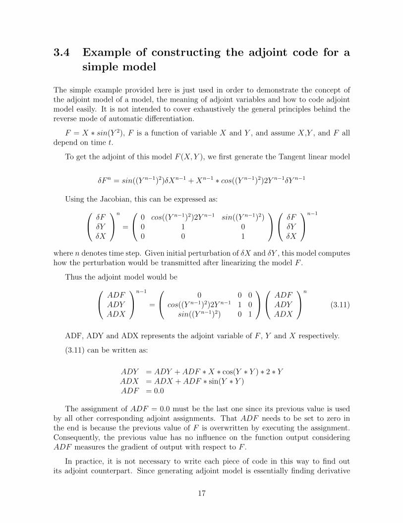
The simple example provided here is just used in order to demonstrate the concept ofthe adjoint model of a model, the meaning of adjoint variables and how to code adjointmodel easily. It is not intended to cover exhaustively the general principles behind thereverse mode of automatic differentiation.

F = X ∗ sin(Y 2), F is a function of variable X and Y , and assume X,Y , and F alldepend on time t.

To get the adjoint of this model F (X, Y ), we first generate the Tangent linear model

δF n = sin((Y n−1)2)δXn−1 +Xn−1 ∗ cos((Y n−1)2)2Y n−1δY n−1

Using the Jacobian, this can be expressed as: δFδYδX

n

=

0 cos((Y n−1)2)2Y n−1 sin((Y n−1)2)0 1 00 0 1

δFδYδX

n−1

where n denotes time step. Given initial perturbation of δX and δY , this model computeshow the perturbation would be transmitted after linearizing the model F .

Thus the adjoint model would be ADFADYADX

n−1

=

0 0 0cos((Y n−1)2)2Y n−1 1 0

sin((Y n−1)2) 0 1

ADFADYADX

n

(3.11)

ADF, ADY and ADX represents the adjoint variable of F , Y and X respectively.

(3.11) can be written as:

ADY = ADY + ADF ∗X ∗ cos(Y ∗ Y ) ∗ 2 ∗ YADX = ADX + ADF ∗ sin(Y ∗ Y )ADF = 0.0

The assignment of ADF = 0.0 must be the last one since its previous value is usedby all other corresponding adjoint assignments. That ADF needs to be set to zero inthe end is because the previous value of F is overwritten by executing the assignment.Consequently, the previous value has no influence on the function output consideringADF measures the gradient of output with respect to F .

In practice, it is not necessary to write each piece of code in this way to find outits adjoint counterpart. Since generating adjoint model is essentially finding derivative

17

in reverse order, some standard procedures can be followed to speed up the process.Some AD tools also exist to do this job though some afterward debugging is very nec-essary, such as the Tangent linear and Adjoint Model Compiler(TAMC), available athttp://www.autodiff.com/tamc.

This adjoint model computes the derivative of ∂F∂X

, ∂F∂Y

(or sensitivity) reversely. Whenintegrated backward in time, this adjoint model would enable us the find out source areathat leads to the final perturbation of ADF .

3.5 Test of accuracy of the adjoint code

The generation of correct adjoint code for the simple example above is trivial. But fora complicated system, it is not an easy task and thus it becomes especially necessaryto test the correctness of adjoint code. The adjoint code is tested using the followingidentity, see Navon et al[12]

< AδX,AδX >=< δX,A∗(AδX) > for any δX (3.12)

where δX is an arbitrary perturbation vector. It is also the input of code A. A representsthe tangent linear code or a segment of it, say a subroutine, a do loop or even a singlestatement. A∗ is the adjoint of A. If (3.12) holds within machine accuracy, it can be saidthat the adjoint is correct versus the tangent linear code.

1. Test of accuracy of the Tangent Linear Model(TLM)To use (3.12) test the correctness of adjoint model, the tangent linear model A isused. Thus first we need to test the correctness of tangent linear model A. Theaccuracy of tangent linear model determines the accuracy of the adjoint model andthe accuracy of the gradient of cost function with respect to the control variables.

To verify A, we use the fact of (3.3) that A is linearization of the model F :

F (X + alpha ∗ δX)− F (X) = A(alpha ∗ δX) +O(alpha2)

where δX is an arbitrary perturbation around X.

We compare the result of TLM with the difference of the twice model call, withand without perturbation respectively. If the TLM is right, then the ratio betweenthese two,

r =F (X + alpha ∗ δX)− F (X)

A∗(alpha ∗ δX)= 1 +O(alpha) (3.13)

will approach zero as α gets close to zero.

18

2. Verification of Adjoint ModelAfter verifying the TLM, We can then use it to test the adjoint model using theadjoin identity:

< AδX,AδX >=< δX,A∗(AδX) > for any X (3.14)

where δX is a perturbation around X. If (3.14) holds within machine precision,then it can be said that the adjoint code is correct with respect to tangent linearmodel.

3. Verification of GradientEven though the TLM and adjoint models are correct, the gradient generated bythe adjoint code needs to be verified because the accuracy of the adjoint gradientnot only depends on the accuracy of the tangent linear and adjoint model, but alsoon the approximation involved in linearizing the cost function (3.3).

Suppose the initial X has a perturbation αh, where α is a small scalar and h is avector of unit length. According to Taylor expansion, we get the cost function:

J(X + αh) = J(X) + αhT 5 J(x) +O(α2)

We can define a function of α as:

Φ(alpha) =J(X + αh)− J(X)

αhT 5 J(X)= 1 +O(α) (3.15)

So as α tends to zero but not close to machine precision, this ratio Φ should beclose to 1. Here the gradient of 5J(X) is calculated by the adjoint model.

This test is usually called α-test.

19

Chapter 4

Numerical Results

In this example, we use the closed option price for SPX on Apr 2ND as our rawdata to estimate the volatility surface. We will calibrate the local volatility functionusing Dupire Equation, i.e., we consider local volatility as a function of strike andmaturity. To simplify the problem, we only look at options with maturity on June18th, and also assume volatility is just a function of strike.

There are a total of 121 options available. But we just use 45 of those optionsthat are near the money (0.9S < K < 1.1S) for two reasons. First, calibration tothe market is usually performed with respect to liquid instruments in the market.Trading volumes for options that are deep in or out of the money are really low.Second, in our numerical test, we find out that the price of options that are deepin or out of the money do not depend on volatility very much: the dependence issmall and they cannot pass neither the tangent linear test nor gradient test.

The SPX on Apr 2ND was 1178.10. The options that we selected for calibrationhad strikes ranging from 1070 to 1300. The interest rate r was 0.0015 which wasattained from 13-week treasury bill and the dividend rate q was assumed to be zero.The computational domain(0, Kmax)× (0, T ) is discretized uniformly into 2000 gridpoints in the K direction and 10 levels in the T direction withKmax = 2000 and T= maturity = 0.21096.

From here we also see the large scale nature of the problem. Dividing the Kdirection of computational domain into 2000 segments means there is a total of1999 parameters that should be estimated because sigma is a function of K. Foreach K, there is a sigma corresponding to it. If sigma is assumed to be a functionof both K and T, the number of parameters to be estimated is even larger.

After constructing the code to solve the Dupire Equation, we use TAMC automaticdifferentiation to generate the code for its tangent linear and adjoint model. Afterdebugging the code, we use the following test to test the validity of the tangentlinear code and adjoint code.

20

4.1 Verification of the Tangent Linear Model

Using (3.5.3), X is volatility in our case. X is constructed by multiplying a randomnumber from (0,1) to each component of X. The ratio r with respect to alpha islisted in table1 and plotted differently in Figure 1 and Figure 2. We can see that asα decreases from 10−2 to 10−11, the ratio r approaches 1 with high accuracy. Whenα is between 10−6 to 10−8, the ratio r is closest to 1.

α r0.1000000000E + 00 0.1032539117E + 010.1000000000E − 01 0.1003277163E + 010.1000000000E − 02 0.1000327956E + 010.1000000000E − 03 0.1000032798E + 010.1000000000E − 04 0.1000003282E + 010.1000000000E − 05 0.1000000326E + 010.1000000000E − 06 0.1000000720E + 010.1000000000E − 07 0.1000000248E + 010.1000000000E − 08 0.9999700354E + 000.1000000000E − 09 0.1000381809E + 010.1000000000E − 10 0.9990800710E + 000.1000000000E − 11 0.1064862770E + 010.1000000000E − 12 0.1665776365E + 010.1000000000E − 13 0.3622784142E + 020.1000000000E − 14 0.4005300720E + 04

Table1

21

Figure1

Figure 2

22

4.2 Transpose Test

< AδX,AδX >= 1630954.41614603

< δX,A∗(AδX) >= 1630954.41614618

We checked the adjoint model segment by segment, do loop by do loop, and sub-routine by subroutine. With double precision, the identity (3.12) is accurate within13 digits. This verified the correctness of adjoint model against TLM.

4.3 Gradient Verification

Instead of minimizing (2.3), the cost function is constructed as a weighted sum ofsquares of the difference:

J(σ) =N

Σi=1

Mi

Σj=1

[(V (S0, 0, Kij, Ti, σ)− V ij)w(ij)]2 (4.1)

where V (S0, 0, Kij, Ti, σ) is the computed option price, V ij = (V bij + V a

ij)/2 is themean of the bid and ask price, w(ij) is a weight that represents our confidence inthe difference between computed price and observed price. This weight is necessaryif we want to give equal weight to price difference between V (S0, 0, Kij, Ti, σ) andV ij for different options. A natural choice of the weight function that describes ourconfidence in an option price is the bid and ask spread of the option. So in ournumerical experiment, we use 1/(bid-ask) as our weight function.

α-test with respect to the above cost function is performed and the result is listedin table 2. Figures 3 and 4 show the variation of Φ(α) and log| 1 − Φ(α) |. Onecan see that as α decreases form 10−5 to 10−15, Φ(α) approaches unity with highaccuracy until α is close to 10−15. This agrees with our expectation that as α getsclose to machine precision, we don’t expect the α-test still holds. This also meansthat for perturbations within the range of 10−5 to 10−15, the gradient calculatedfrom the adjoint model is reliable.

23

α Φ(α)0.100000000000000 9.531840348585277E − 004

1.000000000000000E − 002 2.191575720234569E − 0021.000000000000000E − 003 0.5942171839166921.000000000000000E − 004 1.140538595110661.000000000000000E − 005 1.013543761444591.000000000000000E − 006 1.001348847799271.000000000000000E − 007 1.000134829265371.000000000000000E − 008 1.000013483188521.000000000000000E − 009 1.000001361394671.000000000000000E − 010 1.000000182087329.999999999999999E − 012 1.000000023130881.000000000000000E − 012 1.000004580158791.000000000000000E − 013 1.000028983914801.000000000000000E − 014 0.9990681897791041.000000000000000E − 015 0.9952001114444521.000000000000000E − 016 1.103149379131471.000000000000000E − 017 1.900836778187411.000000000000000E − 018 1.203586606275871.000000000000000E − 019 16.6011945693224

Table2

Figure3

24

Figure4

4.4 Minimization and Discussion

Up to this point, we haven’t performed any regularization yet. We just minimizedthe cost function (4.1). Setting the initial α = 0.5, we performed the minimizationusing LBFGSB. The gradient of the cost function is derived from adjoint model.The cost function is reduced from an order of 105 to an order of 102 within 2minutes. The option prices computed using the optimal volatility are plotted infigure 5. We can see that for options whose strikes are not immediately around thestock price (0.9S < K < 0.95S, 1.05S < K < 1.1S), the computed option pricesapproach the market price well. But for options whose strikes are in immediatevicinity of the stock price(0.95S < K < 1.05S), the computed option prices areabout two or three times the bid-ask spread away from the market prices. Theoptimal volatility σ(K) is plotted with respect to K/S0 in figure 6. We can seethat the curve of σ(K) has the property of a smile: the volatility near the moneyis smaller than the volatility that’s deep in or out of money. When K is either faraway from the money or deep in the money, the optimal volatility doesn’t changetoo much from the initial value.

We also tested the impact of minimization using different initial σ. However, theresult is not as good. The cost function could still be minimized significantlyby a magnitude of 103. But the cost function is much greater than the optimalcost function obtained above. The optimal σ(K) obtained is also not as good

25

by exhibiting some negative values at some region. This means that the successof this large scale minimization problem depends on the initial input, which isin another way of saying that the large scale minimization may get trapped atsome local minima instead of a global minimum. We also tested the minimizationusing other optimization algorithms such as Sequential Quadratic Programmingand Conjugate Gradient method. No better results were obtained either. This maybe due to the fact that the cost function is not as yet regularized, or somethingmore fundamental, the identifiability of the local volatility, which we just realizerecently. These questions lead to our future research.

4.5 Future Research

At the moment this research has not as yet addressed the Tikhonov regularization.The next step will consist in implementing a regularization on the cost function tofind out if we can further reduce the cost function and possibly achieve convergenceto the global minimum.

We observe from Figure 6 that σ(K) for K that is deep in or out of the moneydoesn’t change too much from the initial value. One way to reduce the dimension-ality of the problem may be by introducing nonuniform discretization the compu-tational domain: to have coarse grids when K is deep in or out of the money andto have fine grids when K is near the money. Another alternative for reducing thedimension may be to use adaptive grid generation techniques.

One issue that is probably more fundamental and important comes into our sightrecently: the identifiablity of the local volatility parameters in this inverse problem.The problem of identifiablity in parameter identification is related to the uniquenessproblem in parameter identification. Whether a parameter is identifiable or not hasimportant implications in an inverse problem of parameter identification. When aparameter is identifiable, one can try to develop an algorithm that gives the uniqueexact solution of the inverse problem. When parameters are not identifiable, onemust expect that a procedure of solution of the inverse problem will give a non-unique solution, generally dependent on some parameters or initializers for iterativealgorithms. It is possible sometimes to find methods that lead to a unique solutionof the inverse problem, which in general could be different from the correct solution.Here we just want to briefly introduce the definition of identifiability from [10].

The parameter λ is said to be identifiable if from

λ, λ′ ∈ ∧ad h = Hf (λ) h′ = Hf (λ′) h′ = h

it follows thatλ = λ′

where ∧ad is the admissible parameter subset, and Hf is a mapping from ∧ad tothe observation space. It requires that for every different observation, there is a

26

different set of paramters. This condition, however, cannot be achieved in anypractical problem due to modeling and observation errors.

Relaxation or extension of the definition of identifiablity comes in many formsdepending on the purpose of parameter identification, properties of observationdata, and the nature of the underlying model. Good examples can be found in [28].Identifiablity of this inverse problem will also be another important topic for ourfuture research.

Figure5

Figure6

27

Bibliography

[1] B.DUPIRE. Pricing with a smile. Risk, 7:18–20, 1994.

[2] T.F. COLEMAN and A.VERMA. Reconstructing the unknown local volatility func-tion. The Journal of Computational Finance, 2:77–100, 1999.

[3] R.C.ASTER B.BORCHERS C.THURBER. Parameter Estimation and Invese Prob-lems. Elesvier Academic Press, Burlington, 2005.

[4] E.DERMAN and I.KANI. Riding on a smile. Risk, 7:32–39, 1994.

[5] F.BLACK and M.SCHOLES. The pricing of options and corporate liabilities, journalof political economy. Journal of Political Economy, 81:637–659, 1973.

[6] A. GRIEWANK. On automatic differentiation. In M.IRI and K.TANABE, editors,Mathematical programming: Recent Developments and Applications, pages 83–108.Kluwer Academic Publishers, Dordrecht, 1989.

[7] H.EGGER and H.W.ENGL. Tikhonov regularization applied to the inverse problemof option pricing: convergence analysis and rates. Inverse Problems, 2005.

[8] I.BOUCHOUEV and V.ISAKOV. The inverse problem of option pricing. InverseProblems, 13:L11–L17, 1997.

[9] I.BOUCHOUEV and V.ISAKOV. Uniqueness,stability and numerical methods forthe inverse problem that arises in financial markets. Inverse Problems, 15:R95–116,1999.

[10] I.M.NAVON. Practical and theoretical aspects of adjoint parameter estimationand identifiabiliy in meteorology and oceanography. Dynamics of Atmospheres andOceans, 27:55–59, 1997.

[11] J.C.HULL. Options,futures, and other derivatives. Pearson Education, New Jersey,2009.

[12] I.M.NAVON X.ZOU J.DERBER and J.SELA. Variational data assimilation withan adiabatic version of the nmc spectral model. Monthly Weather Review, 120:1433–1446, 1992.

28

[13] J.JR.BODURTHA and M.JERMAKYAN. Nonparametric estimation of an impliedvolatility surface. The Journal of Computational Finance, 2:29–61, 1999.

[14] L.CAPRIOTTI and M.GILES. Fast correlation greeks by adjoint algorithmic differ-entiation. Risk, 23:79–83, 2010.

[15] L.JIANG Q.CHEN L.WANG and J.E. ZHANG. A new well-posed algorithm torecover implied local volatility. Quantitative Finance, 3:451–457, 2003.

[16] M.GILES and P.GLASSMAN. Smoking adjoints: Fast calculation of greeks in montecarlo calculation. Technical Report, NA-05/15, 2005.

[17] M.RUBINSTEIN. Implied binomial trees. The Journal of Finance, 49:771–818,1994.

[18] P.C.HANSEN. Rank-Deficient and Discrete Ill-Posed Problems: numerical aspects oflinear inversion. Society for Industrial and Applied Mathematics(SIAM), Philadel-phia, 1998.

[19] R.GIERING. Tangent linear and adjoint biogeochemical models. In P.RaynerN.Mahowald R.G.Prinn D.E.Hartley P.Kasibhatla, M.Heimann, editor, Inversemethods in global biogeochemical cycles, pages 33–47. American Geophysical Union,Washington DC, 2000.

[20] R.GIERING and T.KAMINSKI. Recipes for adjoint code construction. ACM onTransactions on Mathematical Software, 24:437–474, 1998.

[21] M.AVELLANEDA C.FRIDMAN R.HOLEMS and D.SAMPERI. Calibratingvolatility surface via relative entropy minimization. Applied Mathematical Finance,4:667–686, 1997.

[22] R.LAGNADO and S.OSHER. Reconciling difference. Risk, 10:79–83, 1997.

[23] R.LAGNADO and S.OSHER. A technique for calibrating derivative security pricingmodels: numerical solution of an inverse problem. The Journal of ComputationalFinance, 1:13–25, 1998.

[24] R.MERTON. Option pricing when underlying stock returns are discontinuous. Jour-nal of Financial Econommics, 3:125–44, 1976.

[25] S.CREPEY. Calibration of the local volatility in a generalized black-scholes modelusing tikhonov regularization. SIAM on Journal of Mathematical Analysis, (5), 2003.

[26] S.CREPEY. Delta-hedging vega risk. Quantitative Finance, 4(5), 2004.

[27] S.L.HESTON. A closed-form solution for options with stochastic volatility withapplication to bond and currency options. The Review of Financial Studies, 6:327–343, 1993.

29

[28] N.Z. SUN and W.W.-G. YEH. Coupled inverse problems in groundwater modeling2. identifiability and experimental design. Water Resourses Research, 26(10):2527–2540, 1990.

[29] G. TURINICI. Calibration of local volatility using the local and implied instanta-neous variance. The Journal of Computational Finance, 13(2), 2009.

[30] Y.ACHDOU and O.PIRONNEAU. Computational Methods for Option Pricing. So-ciety for Industrial and Applied Mathematics(SIAM), Philadelphia, 2005.

30