sequential tikhonov regularization: an alternative - diva portal

FachbeitragEshagh, Sequential Tikhonov Regularization: An Alternative Way for Integral Inversion …

113136. Jg. 2/2011 zfv

AbstractNumerous regularization methods exist for solving the ill-posed problem of downward continuation of satellite grav-ity gradiometry (SGG) data to gravity anomaly at sea level. Generally, the use of a dense set of data is recommended in the downward continuation. However, when such dense data are used some of the regularization methods are not efficient and applicable. In this paper, a sequential way of using the Tikhonov regularization is developed for solving large systems and compared to methods of direct truncated singular val-ue decomposition and iterative methods of range restricted minimum residual, algebraic reconstruction technique, ν and conjugate gradient for recovering gravity anomaly at sea level from the SGG data. Numerical studies show that the sequen-tial Tikhonov regularization is comparable to the conjugate gradient and yields similar result.

ZusammenfassungZur Stabilisierung des unterbestimmten Problems der har-monischen Fortsetzung von Satellitengradiometriedaten zu Schwere anoma lien auf Geoidhöhe gibt es unterschiedliche Regularisierungsmethoden. Im Allgemeinen wird die Verwen-dung eines räumlich dichten Datensatzes für die harmonische Fortsetzung nach unten empfohlen. Aber für diesen Fall sind einige der Regularisierungsverfahren numerisch ineffizient und daher nicht gut anwendbar. In diesem Beitrag wird ein sequenzielles Verfahren der Tikhonov-Regularisierung für die Fortsetzung großer Datensätze vorgestellt und mit direkten Regularisierungsmethoden, wie der abgeschnittenen/abge-brochenen Singulärwertzerlegung, sowie iterativen Methoden, wie der entfernungsbeschränkten Minimierung der Residuen, der algebraischen Rekonstruktionsmethode, der ν Methode und der Methode der konjugierten Gradienten, verglichen. Numerische Untersuchungen zeigen, dass die sequenzielle Tikhonov-Regularisierung mit der Methode der konjugierten Gradienten vergleichbar ist und zu gleichwertigen Ergebnis-sen führt.

Keywords: bias-correction, integral inversion, iterative regularization, Krylov subspaces, Tikhonov regularization

1 Introduction

The gravity field and steady-state ocean circulation ex-plorer (GOCE) (ESA 1999, 2008) is the recent European Space Agency satellite mission which uses the satellite gravity gradiometry (SGG) technique. The main product

of this mission will be a set of spherical harmonic coeffi-cients of the Earth’s gravity field and their corresponding errors to degree and order 200 corresponding to a spatial resolution of 0.9° × 0.9° (100 km × 100 km). This set is expected to deliver the geoid and gravity anomalies with accuracies of 1–2 cm and 1 mGal, respectively from joint inversion of SGG and satellite-to-satellite tracking data. GOCE measures the full tensor of gravitation, contain-ing second-order partial derivatives of the geopotential, in the gradiometer reference frame, second by second, during its life. However, it should be stated that the full tensor of gravitation is not measured with the same ac-curacy and there are highly sensitive and less sensitive gradiometer axes. GOCE will provide a very dense set of the SGG data all over the globe, except polar gaps. The SGG data of GOCE can be used directly to recover gravity anomalies at sea level.

The problem of determining the gravity anomalies at sea level from SGG data was the issue investigated by Reed (1973). He used the second-order partial derivatives of the extended Stokes formula to present the integral relation between gravity anomaly and the SGG data and inverted them to recover the gravity anomaly. Since in-version of such integral formulas is an ill-posed problem he used some a priori constraints for regularization of the integral equations. Later on, this idea was followed by Xu (1992) who presented a technique to invert the integral formulas without a priori information and it was further investigated in Xu (1998) by comparing it with some direct regularization methods. Koch and Kusche (2002) developed an iterative method for simultaneous estimation of variance components and regularization parameter. Kotsakis (2007) used the integral inversion for recovering the gravity anomaly at sea level by a cova-riance-adaptive method. Eshagh (2009) used the integral inversion method for the recovery of the anomalies from full gravitational tensor. Xu (2009) presented a method based on generalized cross validation for simultaneous estimation of variance components and regularization of system of equations. Janak et al. (2009) carried out the inversion of full gravitational tensor to gravity anomalies using the truncated singular value decomposition. Inver-sion of stochastically modified integral of second-order radial derivative of the extended Stokes formula was done by Eshagh (2011a). Regional gravity field recovery from SGG data using least-squares collocation was done by Tscherning (1988, 1989) and Arabelos and Tscherning (1990, 1993, 1995 and 1999). Tscherning et al. (1990) studied three different methods of regional gravity field recovery: least-squares collocation, Fourier Transform

Sequential Tikhonov Regularization: An Alternative Way for Integral Inversion of Satellite Gradiometric Data

Mehdi Eshagh

Fachbeitrag Eshagh, Sequential Tikhonov Regularization: An Alternative Way for Integral Inversion …

114 zfv 2/2011 136. Jg.

and the integral approach which was further developed by Eshagh (2011b).

In each one of the reviewed studies one regularization method was considered for inversion of integral formu-las. However, it is obvious that there are more regular-ization methods with their own benefits. In this study, the goal is to investigate some of these regularization methods, in the same conditions, to see which one of them is suitable for recovering gravity anomalies from the SGG data. These regularization methods are classi-fied into two main groups of direct and iterative. Here, direct methods of Tikhonov regularization (TR) (Tikhonov 1963) and the truncated singular value decomposition (TSVD) (Hansen 1998) are considered as well as iterative methods of ν (Brakhage 1987), algebraic reconstruction technique (ART) (Kaczmarz 1937), the range restricted generalized minimum residual (RRGMRES) (Calvetti et al. 2000) and conjugate gradient (CG) (Hanke 1995). Also a new strategy to use the TR in a sequential way is simply developed and named sequential TR (STR), which is ap-plied for recovering the gravity anomalies at sea level from the SGG data.

2 Second-order radial derivative of Stokes’ formula

The second-order radial derivative of geopotential is the simplest and the most important element of the gravita-tional tensor. It is simple because its mathematical for-mulation is easier than the other gradients, and it is im-portant as it has the most power with respect to the other gradients. Let the following estimator for this gradient at satellite level be (Reed 1973):

( ) ( ) ( )0

,4rr rr

RT P S r g Q d

σ

ψ σπ

= ∆∫∫ , (1a)

where ( ) 2 2rrT P T r= ∂ ∂ , T stands for disturbing potential,

R is the mean radius of the Earth, Dg (Q) is the gravity anomaly at the integration point Q, y is the geocentric angle between the computation and integration points P and Q, s0 cap size of integration as we are integrating over a spherical cap (which is an assumption with respect to the realistic full scale inversion problem) and refer to it later in the numerical example, and ( ) ( )2 2, ,rrS r S r rψ ψ= ∂ ∂ (where ( ),S r ψ is the extended Stokes’ function) is the kernel of integral (Reed 1973, Eq. (5.35)):

( ) ( ) ( )23 2

2 5 3 3

3 1 4 1 10 1 cos, 1 cos 18 2 3 cos 15 6 ln

2rr

tt t t DS r t D t

R D D D Dψ

ψ ψ ψ − + − + = − − − − − + − +

( ) ( ) ( )23 2

2 5 3 3

3 1 4 1 10 1 cos, 1 cos 18 2 3 cos 15 6 ln

2rr

tt t t DS r t D t

R D D D Dψ

ψ ψ ψ − + − + = − − − − − + − +

,

(1b)

where t R r= , 21 2 cosD t tψ= − + and r is the geo-centric distance of P.

Eq. (1a) is the Fredholm integral equation of the first kind, and inversion of such an integral is an ill-posed problem. The integral in the right hand side of this equa-tion should be discretized and solved. Let us present the discretized integral (1a) in the following matrix form:

= −Ax L ε , { } 20E T σ= Qεε and { }E 0=ε , (2)

where A is the n × m coefficient matrix (right hand side of Eq. (1a)), L is the n × 1 vector of rrT (left hand side of Eq. (1a)), e is the n × 1 vector of error of L, x is the m × 1 vector of unknown parameters or the gravity anomalies at sea level, E stands for statistical expectation operator,

20σ is the a priori variance factor which is equal to 1 and

Q is the variance-covariance matrix of observations which is considered an identity matrix in this study. Since the matrix A is derived after discretization of the integral formula (1a), e. g. based on the simple quadra-ture method, then it will be ill-conditioned. This means that the condition number of A will be large so that by inverting the system of equations (2), the errors of ob-servables are amplified and destroy the solution. This unwanted property can be controlled by regularization which means to neglect the high frequencies of the solu-tion. Numerous methods have been presented for solving such an ill-posed problem. These methods are so-called regularization. The next section will present an overview for some of them.

3 A conceptual overview of regularization methods

The regularization methods are divided into two catego-ries of direct and iterative. Iterative methods are impor-tant as they avoid the direct inversion of the system of equations. This is the reason that the iterative methods are recommended for large systems. In spite of the it-erative methods, the direct methods solve the system by direct inversion of its coefficients matrix, which is a com-plicated problem when it is large and ill-conditioned. In the following sections, some of the direct and iterative methods are reviewed.

3.1 Direct methods

This subsection presents two well-known methods of TSVD and TR for solving ill-conditioned system of equa-tions. Both of these methods have a shortcoming of working with large matrices. In the following, these two methods are briefly introduced.


115136. Jg. 2/2011 zfv

3.1.1 Truncated singular value decomposition

The main idea of the truncated singular value decomposi-tion (TSVD) comes from the fact that the small eigenval-ues of the coefficients matrix of system are removed and those parts of solution relating to these small eigenvalues are neglected in the final solution. In fact, the high fre-quencies of the solutions are removed and a smoothed solution is sought. In order to explain the concept of the TSVD, the singular value decomposition of the matrix A is considered:

T=A U VΛ , (3a)

where U is an n × n orthogonal matrix with UUT = In, and V is an m × m orthogonal matrix with VVT = Im, I stands for the identity matrix with dimensions of n or m and L is an n × m matrix containing eigenvalues (singular val-ues) in a decreasing order. U and V contain eigenvectors of A and they play the role of the base functions for A. Substituting Eq. (3a) into Eq. (2) and solve the result for x yields:

1

TnT i

ii i

uv

λ+

=

= = ∑ Lx V U LΛ , (3b)

where L+ is the pseudo inverse of L, li is the eigenvalues of A, T

iu and νi are the vectors constructing the orthogo-nal matrices U and V.

Eq. (3b) is the least-squares solution of the system of equations (2) in the spectral form. Since the singular value is located in the denominator of the solution, therefore, when it is small, this component of the solution will be amplified and since L is erroneous, its error is amplified as well. The idea of the TSVD is not to use all the spectra of the solution and truncate the series (3b) to k instead of n. In this case, a smooth solution is obtained. One can mention that the minimization problem of the TSVD is:

{ }1 22span , , ,

mink∈

−x v v v

L Ax

, (3c)

where 2• stands for the L2-norm. Eq. (3c) means that x

is obtained from a combination of the bases v1, v2, …, vk and k means that the solution is constructed by k bases. The main issue in the TSVD is the proper selection of the truncation number k. Different methods have been pre-sented for estimating k such as generalized cross valida-tion (Wahba 1976), L-curve (Hansen 1998), quasi-optimal method (Hansen 2007), discrepancy principle (cf. Scherzer 1993), the monotone error rule (Hämarik and Taytenhahn 2001), normalized cumulative periodogram (cf. Diggle 1991 or Mojabi and LoVetri 2008).

3.1.2 Tikhonov regularization

Tikhonov (1963) was one of the earliest persons started solving ill-posed problems. His method is summarized in the following minimization problem:

( )22 2

min α− +Ax L x , (4a)

where a is the regularization parameter. The solution of the above minimization problem is obtained by solving the following system of equations:

( )2T Tα+ =A A I x A L, (4b)

where I is the identity matrix. Tikhonov’s idea is to add a small positive number to the diagonal elements of the coefficients matrix of the normal system of equations for stabilizing it. The main important issue in this method is the proper choice of this small positive number or the regularization parameter. Therefore the regularized solu-tion of Eq. (2) will be:

( ) 12reg

T Tα−

= +x A A I A L. (4c)

Due to adding the regularization parameter the solution will be biased. This bias is the penalty to pay for stabiliza-tion purpose and it is presented by the following formula (Xu et al. 2006, Eshagh 2009):

( ) ( ) 12 2regBias T −

= − +x A A I xα α . (4d)

The regularization parameter a can be estimated by L-curve, generalized cross validation (Wahba 1976) or quasi-optimal method (Hansen 2007).

3.1.3 Sequential Tikhonov regularization

The shortcoming of the TR is to invert a large coefficient matrix which is time consuming and sometimes impos-sible. Different approaches proposed for using the TR for large systems such as Arnoldi-TR (Lewis and Reichel 2008) and Lanczos bidiagonalization TR (Björck 1988, Calvetti et al. 2000, 2003, Golub and von Matt 1997, Kilmer and O’Leary 2001 and O’Leary and Simmons 1981). These versions of the TR take advantage of some matrix fac-torizations like Lanczos bidiagonalization (Björck 1988) and Arnoldi decomposition (Saad 1996) to the system of equations and work with structure of the system. The idea of applying the TR on the normal equations is not relevant for two reasons: a) increase of the condition number by power 2 which makes the normal system more unstable than the system itself, b) loss of some physical properties of A and L due to being multiplied by AT (cf. Maitre and Levy 1983). However, the problem of solving the ill-posed problems using the TR is possible in another simple way if the number of unknown parameters is not very large. In this case, the TR method can be used sequentially so that


116 zfv 2/2011 136. Jg.

working with large number of observations is possible. This method is named sequential TR (STR) in this study. The idea of the STR method is very similar to the sequen-tial least-squares adjustment (see e. g. Cooper 1987). In this case the system of equations is partitioned into small subsystems. One system is solved and the improvements of the solution due to the other systems and observations are computed and implied on the former solution sequen-tially. The beauty of the STR is its capability to work with large systems without estimating the regularization parameter from normal equations. In order to explain the idea, let us assume that the system of equations is divided into two subsystems:

= −

A Lx

A Lεε

1 1 1

2 2 2

, (5a)

where A1 and A2 are the coefficient matrices of the first and the second subsystems. The vector of observation L is divided into L1 and L2 with corresponding errors e1 and e2.

The TR solution of the first system will be:

( ) 11 2reg 1 1 1 1

T Tα−

= +x A A I A L . (5b)

Now assume that the regularization parameter was al-ready estimated from the first system. Therefore the solu-tion of both systems together will be:

( ) ( )12 2reg 1 1 2 2 1 1 2 2

T T T Tα−

= + + +x A A A A I A L A L . (5c)

This means that the same regularization parameter as that was used in the first systems (5b) is used to estimate

2regx . In this case, the system of equations will not be ill-

conditioned but the regularization parameter has not the best value. It is straightforward to write Eq. (5c) in the following form:

( ) ( )12 1 2 1reg reg 1 1 2 2 2 2 2 reg

T T T Tα−

= + + + −x x A A A A I A L A x . (5d)

The solution 1regx contains a bias due to the TR, but ac-

cording to Eq. (4d) this bias can be estimated by consid-ering 1

regx as the approximate value of x. Xu et al. (2006) mentioned that, in this case, a second-order bias occurs but its power is smaller than the first-order one. Therefore removing the bias can improve the solution. Consequent-ly, the following STR estimator is derived:

( ) ( ) ( )12 1 1 2 1reg reg reg 1 1 2 2 2 2 2 regBias T T T Tα

−= − + + + −x x x A A A A I A L A x

( ) ( ) ( )12 1 1 2 1reg reg reg 1 1 2 2 2 2 2 regBias T T T Tα

−= − + + + −x x x A A A A I A L A x (5e)

and

( ) ( ) 12 2 2reg 1 1 2 2Bias T T −

= − + +x A A A A I xα α . (5f)

This idea can be generalized to the case where the system is divided into k + 1 sub matrices:

( ) ( )11

1 2reg reg reg 1 1 1 reg

1

Biask

k k k T T T ki i k k k

i

α−+

++ + +

=

= − + + − ∑x x x A A I A L A x

( ) ( )

111 2

reg reg reg 1 1 1 reg1

Biask

k k k T T T ki i k k k

i

α−+

++ + +

=

= − + + − ∑x x x A A I A L A x

(5g)

and

( )11

1 2 2reg

1

Biask

k Ti i

i

−++

=

= − + ∑x A A I xα α . (5h)

3.2 Iterative methods

Here the iterative methods are divided into two groups: a) the classical iterative methods and b) the methods based on Krylov subspaces. In this study, the former class includes the ν method and the algebraic reconstruction technique (ART) and the latter consists of the range re-stricted generalized minimum residual (RRGMRES) and conjugate gradient (CG).

3.2.1 Classical iterative methods

In this section, the ν method (Brakhage 1987) and ART (Kaczmarz 1937) are presented. For more details about these methods the reader is referred to the reference list.

3.2.1.1 The ν method

This method is an extension of the Landweber method (Engl and Groetsch 1987). Generally, the Landweber it-erative method is presented by:

( )1 1k k T kω− −= + −x x A Ax L . (6a)

The classical Landweber method is to select ( )TFω = A A where F is a rational function of AT A. Depending on the choice of w, different cases for the Landweber methods are derived. For example if one selects ( ) 12Tω α

−= +A A I

the method will be the iterative Tikhonov regularization. The ν method is a special case of the Landweber meth-od which accelerates the method by replacing xk–1 by a weighted average of some last iterates and allowing w to depend on k. This method was presented by Brakhage (1987) which is a two-step procedure of the form (Hansen 1998):

( ) ( )1 2 11k k k T kk k k

− − −= + − + −x x x A Ax Lµ µ ω , (6b)

where

( )( )( )( )( )( )

1 2 3 2 2 11

2 1 2 4 1 2 2 3k

k k k v

k v k v k vµ

− − + −= +

+ − + − + − , (6c)


117136. Jg. 2/2011 zfv

( )( )( )( )4 2 2 1 1

2 1 2 4 1k

k v k

k v k v

νω

+ − + −=

+ − + − (6d)

and 0 < ν < 1.

3.2.1.2 Algebraic reconstruction technique

The algebraic reconstruction technique (ART) is called a row-action method as each row of the matrix A is used at a time. This method is suitable when A has large dimen-sions. In this method, in each iteration involves a step through the rows of A of the form (Hansen 1998):

11 2

2

Ti i k

k k i

i

−−

−= +

L a xx x a

a , (7)

where L1 is the i-th components of L and ai is the i-th row of A.

3.2.2 Krylov subspaces-based methods

In the Krylov subspaces-based methods (Hansen 1998), the following minimization problem is solved:

2min

kK∈−

xL Ax . (8a)

Eq. (8a) means that the residual is minimized so that the solution is in the k-dimensional subspaces Kk. This solu-tion subspace can be represented by Krylov subspaces. A Krylov space of order k, generated by an n-by-n ma-trix A and a vector L of dimension n is the linear sub-space spanned by the images of L under the first k powers of A. The iterative solution of the system can be presented in the following form (Jensen and Hansen 2007):

( )k k ′= Φx B B L (8b)

where Fk(B) is a polynomial of degree k-1 with the ma-trix B. B and B´ are defined based on each method and its corresponding Krylov subspaces. xk stands for k-th iterated solution. Eq. (8b) shows that the solution will be a combination of B and B´L, or in other words; in Krylov subspaces:

( ) { }1, span , , , kkK −′ ′ ′ ′∈ =x B B L B L BB L B B L . (8c)

3.2.2.1 Range restricted generalized minimum residual method

The range restricted generalized minimum residual (RRGMRES) was proposed by Calvetti et al. (2000) for solving the system of equations with a squares coefficient matrix. They modified the generalized minimum residual (GMRES) method (Saad and Schultz 1986) by restricting

the solution to range of the coefficient matrix of system of equations. If this iterative method is applied for solv-ing a system, it will yield the least-squares solution of the system and when it is applied for a singular system it yields its minimum norm least-squares solution. Cal-vetti et al. (2000) proved that RRGMRES has an intrinsic regularization property and the vector L is damped by the ill-conditioned matrix A. If these methods are applied for solving ill-conditioned systems the iterative solutions will converge to the minimum-norm least-squares solu-tion. However, the first few iterated solutions can be con-sidered as a regularized solution as we are not interested in the convergence of the solution to the minimum-norm least-squares one. In fact the long wavelength structure of the solution is constructed by the first iterations and by iterating the solution its higher frequencies are obtained. In singular value point of view, one can say that the first large singular value components of the solution contrib-ute more strongly to the solution than the component corresponding to small singular values (Jensen and Han-sen 2007). A study of Hansen and Jensen (2006) showed that these iterative regularization methods are superior to minimum residual and GMRES as they have a better noise suppression property.

Generally, the GMRES problems are solved using the Arnoldi decomposition (Saad 1996):

1k k k+=AV V H (9a)

where ( )1 1 2 1 1k k n k+ + × += V v v v has orthogonal

columns i. e. 1 1 1Tk k k+ + +=V V I which span the Krylov sub-

spaces Kk (A,L) and ( )( )1k k k+ ×H is of Hessenberg-type,

which an almost triangular matrix. The upper and lower triangular Hessenberg matrices have zero elements below the first sub-diagonal and above the first super-diagonal elements, respectively. In order to see how to generate these matrices see e. g. Calvetti et al. (2000). By selecting the k=x V y and substituting it into Eq. (2) the following minimization problem can be achieved:

( ) 12 2, Rmin min

kk

k kK +∈ ∈− = −

x A L yL Ax L V H y . (9b)

Eq. (9b) shows that the Arnoldi decomposition trans-fers the solution space from Kk (A,L) into y ∈ Rk which is simpler to solve as the problem is converted to an ordinary minimization problem. Once y is estimated x will be obtained from x = Vky. The Krylov subspaces of both methods are Kk (A,L). Now if the subspace Kk (A,AL) is considered for this method, the RRGMRES is derived which have somehow a regularization property due to multiplication of A to L in the subspaces. As Calvetti et al. (2000) mentioned the matrix ( )1R k k

k+ ×∈H will not be

ill-conditioned if the Arnoldi decomposition starts with AL vector instead of A. This is the regularization philoso-phy behind the RRGMRES method. According to Jensen


118 zfv 2/2011 136. Jg.

and Hansen (2007), the effect of the polynomial Fk (B) in these methods is to ‘kill’ the large components of UT L, U is the eigenvector of A, by being small for these large components.

3.2.2.2 Conjugate gradient

The conjugate gradient (CG) method was designed for solving the system of equations having symmetric and sparse coefficient matrix. It can be used for solving any type of systems, but if one desires to have a least-squares solution, it should be applied for the un-regularized nor-mal equations:

T T=A Ax A L . (10a)

The minimization problem here will be the same as that presented in Eq. (8a) considering B = AT A and B´ = AT in Eq. (8c).

In CG the components related to the large singular val-ues converge faster than those involved with small ones. This is the reason the CG has an intrinsic regularization property (Hansen 2007). In geometrical point of view, the minimization problem creates concentric ellipses around the solution and in each iteration a gradient to that ellipse passing from the iterative solution is generated towards the final solution (Bouman 1998) so that the gradient is orthogonal to all previous ones.

Two vectors are conjugate if they are orthogonal with respect to inner product. If pk is the sequence of orthogo-nal directions, then the solution of the system can be expanded in terms of these directions which can play the role of base function for the solution:

1

k

i ii

α=

= ∑x p , (10b)

where i stands for iteration and ai is the coefficients of the expansions. n will be maximum number of iterations. Substituting Eq. (10b) into Eq. (10a) yields:

1

nT T T

i ii

α=

= =∑A Ax A Ap A L . (10c)

Pre-multiplying Eq. (10c) by pk and further simplifica-tions yield:

T Tk

k T Tk k

α =p A L

p A Ap . (10d)

CG needs an initial value x0 which can be considered as zero without loss of generality. However, the solution is sought in such a way that the following function is minimized:

( ) 12

T T T TF = −x x A Ax x A L . (10e)

Since F (x) should be a minimizer, then its gradient should be p0 = Ax0 – L. By having this gradient one can obtain ai using Eq. (10d) and

1

Ti i

k k iT Ti k i i

+≤

= −∑ p Arp r p

p A Ap , (10f)

1 1 1k k k kα+ + += +x x p . (10g)

Eq. (10b) presents the solution by a series which is con-structed iteratively by adding its frequencies step-by-step. The first iterations include the low frequencies and the high frequencies, infected to the observation noise, are added by iterating the solution. By truncating the se-ries of Eq. (10b) to k, which means to stop iteration before convergence of the solution, the infected higher frequen-cies are neglected and a smooth solution is achieved. This is the regularization property of the CG method.

4 Numerical studies

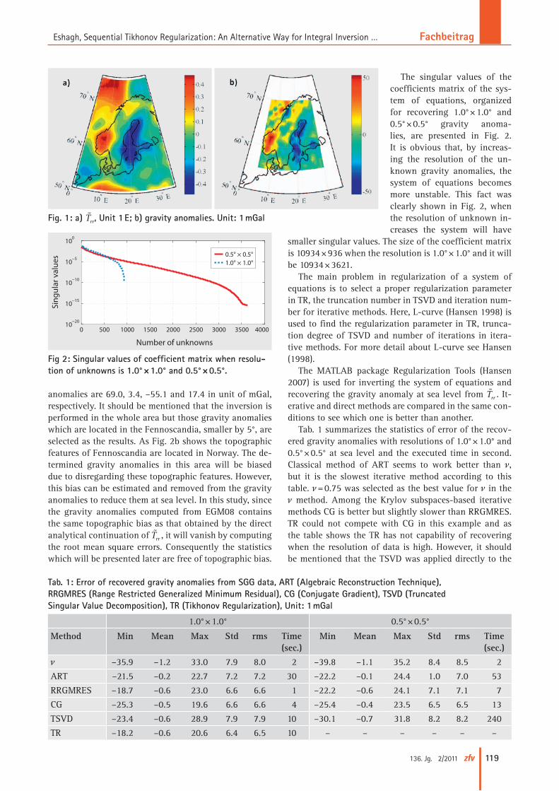
In order to test quality of the aforementioned regular-ization methods, a simulation test is done. The EGM08 geopotential model (Pavlis et al. 2008) is used as true gravity model for generating rrT and the gravity anoma-lies at sea level. The problem is to recover the gravity anomalies from inversion of the second-order radial de-rivative of disturbing potential rrT in Fennoscandia. This region is limited between the latitudes 55 °N and 70 °N and the longitudes between 5 °E and 30 °E. A larger area by 5° than Fennoscandia is selected for inverting rrT for reducing the effect of the spatial truncation error of the integral formula, namely, this area is limited between the latitudes 50 °N and 75 °N and the longitudes between 0 °E and 35 °E. Figs. (1a) and (1b) show coverage of rrT and the area of recovering gravity anomalies, respec-tively. A 3-month orbit of GOCE is simulated, based on the non-singular formulas for the equations of satellite motion in the presence of a geopotential force, by Es-hagh et al. (2009). It is integrated with a rate of 10 s at an approximate altitude of 250 km above the Earth surface. Those satellite’s passes over Fennoscandia are separated from the whole orbit over this area. The goal is to re-cover the gravity anomaly with resolutions of 1.0° × 1.0° and 0.5° × 0.5° in Fennoscandia from the generated rrT . In order to test the quality of the recovered anomalies they are compared to the corresponding anomalies com-puted from EGM08. A coloured noise is generated for rrT by passing a white noise with a standard deviation of 0.02 E through an auto-regressive moving average filter of degree 2 and order 1; i. e. ARMA (2,1) (Kless et al. 2003).

The maximum, mean, minimum and standard devia-tion of rrT are 0.53, 0.04, –0.05 and 0.2 in Eötvös units, re-spectively and the corresponding statistics for the gravity


119136. Jg. 2/2011 zfv

anomalies are 69.0, 3.4, –55.1 and 17.4 in unit of mGal, respectively. It should be mentioned that the inversion is performed in the whole area but those gravity anomalies which are located in the Fennoscandia, smaller by 5°, are selected as the results. As Fig. 2b shows the topographic features of Fennoscandia are located in Norway. The de-termined gravity anomalies in this area will be biased due to disregarding these topographic features. However, this bias can be estimated and removed from the gravity anomalies to reduce them at sea level. In this study, since the gravity anomalies computed from EGM08 contains the same topographic bias as that obtained by the direct analytical continuation of rrT , it will vanish by computing the root mean square errors. Consequently the statistics which will be presented later are free of topographic bias.

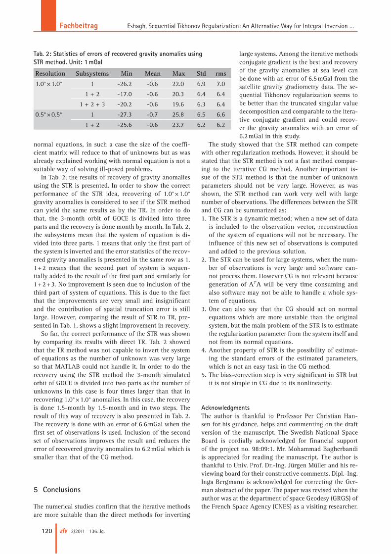
The singular values of the coefficients matrix of the sys-tem of equations, organized for recovering 1.0° × 1.0° and 0.5° × 0.5° gravity anoma-lies, are presented in Fig. 2. It is obvious that, by increas-ing the resolution of the un-known gravity anomalies, the system of equations becomes more unstable. This fact was clearly shown in Fig. 2, when the resolution of unknown in-creases the system will have

smaller singular values. The size of the coefficient matrix is 10934 × 936 when the resolution is 1.0° × 1.0° and it will be 10934 × 3621.

The main problem in regularization of a system of equations is to select a proper regularization parameter in TR, the truncation number in TSVD and iteration num-ber for iterative methods. Here, L-curve (Hansen 1998) is used to find the regularization parameter in TR, trunca-tion degree of TSVD and number of iterations in itera-tive methods. For more detail about L-curve see Hansen (1998).

The MATLAB package Regularization Tools (Hansen 2007) is used for inverting the system of equations and recovering the gravity anomaly at sea level from rrT . It-erative and direct methods are compared in the same con-ditions to see which one is better than another.

Tab. 1 summarizes the statistics of error of the recov-ered gravity anomalies with resolutions of 1.0° × 1.0° and 0.5° × 0.5° at sea level and the executed time in second. Classical method of ART seems to work better than ν, but it is the slowest iterative method according to this table. ν = 0.75 was selected as the best value for ν in the ν method. Among the Krylov subspaces-based iterative methods CG is better but slightly slower than RRGMRES. TR could not compete with CG in this example and as the table shows the TR has not capability of recovering when the resolution of data is high. However, it should be mentioned that the TSVD was applied directly to the

Fig. 1: a) rrT , Unit 1 E; b) gravity anomalies. Unit: 1 mGal

0 500 1000 1500 2000 2500 3000 3500 400010−20

10−15

10−10

10−5

100

Number of unknowns

Sing

ular

val

ues 0.5° × 0.5°

1.0° × 1.0°

Fig 2: Singular values of coefficient matrix when resolu-tion of unknowns is 1.0° × 1.0° and 0.5° × 0.5°.

Tab. 1: Error of recovered gravity anomalies from SGG data, ART (Algebraic Reconstruction Technique), RRGMRES (Range Restricted Generalized Minimum Residual), CG (Conjugate Gradient), TSVD (Truncated Singular Value Decomposition), TR (Tikhonov Regularization), Unit: 1 mGal

1.0° × 1.0° 0.5° × 0.5°

Method Min Mean Max Std rms Time (sec.)

Min Mean Max Std rms Time (sec.)

ν –35.9 –1.2 33.0 7.9 8.0 2 –39.8 –1.1 35.2 8.4 8.5 2

ART –21.5 –0.2 22.7 7.2 7.2 30 –22.2 –0.1 24.4 1.0 7.0 53

RRGMRES –18.7 –0.6 23.0 6.6 6.6 1 –22.2 –0.6 24.1 7.1 7.1 7

CG –25.3 –0.5 19.6 6.6 6.6 4 –25.4 –0.4 23.5 6.5 6.5 13

TSVD –23.4 –0.6 28.9 7.9 7.9 10 –30.1 –0.7 31.8 8.2 8.2 240

TR –18.2 –0.6 20.6 6.4 6.5 10 – – – – – –


120 zfv 2/2011 136. Jg.

normal equations, in such a case the size of the coeffi-cient matrix will reduce to that of unknowns but as was already explained working with normal equation is not a suitable way of solving ill-posed problems.

In Tab. 2, the results of recovery of gravity anomalies using the STR is presented. In order to show the correct performance of the STR idea, recovering of 1.0° × 1.0° gravity anomalies is considered to see if the STR method can yield the same results as by the TR. In order to do that, the 3-month orbit of GOCE is divided into three parts and the recovery is done month by month. In Tab. 2, the subsystems mean that the system of equation is di-vided into three parts. 1 means that only the first part of the system is inverted and the error statistics of the recov-ered gravity anomalies is presented in the same row as 1. 1 + 2 means that the second part of system is sequen-tially added to the result of the first part and similarly for 1 + 2 + 3. No improvement is seen due to inclusion of the third part of system of equations. This is due to the fact that the improvements are very small and insignificant and the contribution of spatial truncation error is still large. However, comparing the result of STR to TR, pre-sented in Tab. 1, shows a slight improvement in recovery.

So far, the correct performance of the STR was shown by comparing its results with direct TR. Tab. 2 showed that the TR method was not capable to invert the system of equations as the number of unknown was very large so that MATLAB could not handle it. In order to do the recovery using the STR method the 3-month simulated orbit of GOCE is divided into two parts as the number of unknowns in this case is four times larger than that in recovering 1.0° × 1.0° anomalies. In this case, the recovery is done 1.5-month by 1.5-month and in two steps. The result of this way of recovery is also presented in Tab. 2. The recovery is done with an error of 6.6 mGal when the first set of observations is used. Inclusion of the second set of observations improves the result and reduces the error of recovered gravity anomalies to 6.2 mGal which is smaller than that of the CG method.

5 Conclusions

The numerical studies confirm that the iterative methods are more suitable than the direct methods for inverting

large systems. Among the iterative methods conjugate gradient is the best and recovery of the gravity anomalies at sea level can be done with an error of 6.5 mGal from the satellite gravity gradiometry data. The se-quential Tikhonov regularization seems to be better than the truncated singular value decomposition and comparable to the itera-tive conjugate gradient and could recov-er the gravity anomalies with an error of 6.2 mGal in this study.

The study showed that the STR method can compete with other regularization methods. However, it should be stated that the STR method is not a fast method compar-ing to the iterative CG method. Another important is-sue of the STR method is that the number of unknown parameters should not be very large. However, as was shown, the STR method can work very well with large number of observations. The differences between the STR and CG can be summarized as:1. The STR is a dynamic method; when a new set of data

is included to the observation vector, reconstruction of the system of equations will not be necessary. The influence of this new set of observations is computed and added to the previous solution.

2. The STR can be used for large systems, when the num-ber of observations is very large and software can-not process them. However CG is not relevant because generation of AT A will be very time consuming and also software may not be able to handle a whole sys-tem of equations.

3. One can also say that the CG should act on normal equations which are more unstable than the original system, but the main problem of the STR is to estimate the regularization parameter from the system itself and not from its normal equations.

4. Another property of STR is the possibility of estimat-ing the standard errors of the estimated parameters, which is not an easy task in the CG method.

5. The bias-correction step is very significant in STR but it is not simple in CG due to its nonlinearity.

AcknowledgmentsThe author is thankful to Professor Per Christian Han-sen for his guidance, helps and commenting on the draft version of the manuscript. The Swedish National Space Board is cordially acknowledged for financial support of the project no. 98:09:1. Mr. Mohammad Bagherbandi is appreciated for reading the manuscript. The author is thankful to Univ. Prof. Dr.-Ing. Jürgen Müller and his re-viewing board for their constructive comments. Dipl.-Ing. Inga Bergmann is acknowledged for correcting the Ger-man abstract of the paper. The paper was revised when the author was at the department of space Geodesy (GRGS) of the French Space Agency (CNES) as a visiting researcher.

Tab. 2: Statistics of errors of recovered gravity anomalies using STR method. Unit: 1 mGal

Resolution Subsystems Min Mean Max Std rms

1.0° × 1.0° 1 -26.2 -0.6 22.0 6.9 7.0

1 + 2 -17.0 -0.6 20.3 6.4 6.4

1 + 2 + 3 -20.2 -0.6 19.6 6.3 6.4

0.5° × 0.5° 1 -27.3 -0.7 25.8 6.5 6.6

1 + 2 -25.6 -0.6 23.7 6.2 6.2


121136. Jg. 2/2011 zfv

ReferencesArabelos, D. and Tscherning, C. C.: Simulation of regional gravity field

recovery from satellite gravity gradiometer data using collocation and FFT. Bull. Geod. 64: 363–382, 1990.

Arabelos, D. and Tscherning, C. C.: Regional recovery of the gravity field from SGG and SST/GPS data using collocation. In: Study of the gravity field determination using gradiometry and GPS, Phase 1, Final report ESA Contract 9877/92/F/FL, April, 1993.

Arabelos, D. and Tscherning, C. C.: Regional recovery of the gravity field from satellite gradiometer and gravity vector data using collocation. J. Geophys. Res. 100: No. B11: 22009–22015, 1995.

Arabelos, D. and Tscherning, C. C.: Gravity field recovery from airborne gravity gradiometer data using collocation and taking into account correlated errors. Phys. Chem. Earth (A), 24(1): 19–25, 1999.

Björck, Å.: A bidiagonalization algorithm for solving large and sparse ill-posed systems of linear equations. BIT 28: 656–670, 1988.

Bouman, J.: Quality of regularization methods. DEOS Report 98.2, Delft University Press, Delft, The Netherlands, 1998.

Brakhage, H.: On ill-posed problems and the method of conjugate gra-dient. In: Inverse and ill-posed problems, Engl, H. W. and Groetsche, C. W. (Eds.) Academic Press, London, 1987.

Calvetti, D.; Morigi, S.; Reichel, L.; Sgallari, F.: Tikhonov regularization and the L-curve for large, discrete ill-posed problems. J. Comput. Appl. Math. 123: 423–446, 2000.

Calvetti, D. and Reichel, L.: Tikhonov regularization of large linear problems. BIT 43: 263–283, 2003.

Cooper M. R. A.: Control surveys in civil engineering. Nichols Pub Co (April 1987), 381 pages, 1987.

Diggle P.: Nonparametric comparison of cumulative periodograms. Appl. Statist. 40(3): 423–434, 1991.

Engl, H. W. and Groetsch, C. W.: Inverse and ill-posed problems. Aca-demic Press, London, 1987.

ESA: GOCE: one of ESA’s most challenging missions yet, ESA Bulletin, February, 2008.

ESA: Gravity Field and Steady-State Ocean Circulation Mission. ESA SP-1233(1), Report for mission selection of the four candidate earth explorer missions. ESA Publications Division, pp. 217, July 1999.

Eshagh, M.: On satellite gravity gradiometry. Doctoral dissertation in Geodesy, Royal Institute of Technology (KTH), Stockholm, Sweden, 2009.

Eshagh, M.: Inversion of satellite gradiometry data using statistically modified integral formulas for local gravity field recovery, Adv. Space Res. 47: 74-85, 2011a.

Eshagh, M.: On integral approach to regional gravity modelling from satellite gradiometric data, Acta Geophys. 59(1): 29-54, 2011b.

Eshagh, M.; Abdollahzadeh, M. and Najafi-Alamdari, M.: Simplification of geopotential perturbing force acting on a satellite. Artif. Satel., 43(2): 45–64, 2009.

Golub, G. H. and von Matt, U.: Tikhonov regularization for large scale problems. In: Golub, G. H.; Lui, S. H.; Luk, F. and Plemmons, R. (Eds), Workshop on Scientific Computing, Springer, New York, pp. 3–26, 1997.

Hanke, M.: Conjugate gradient type methods for ill-posed problems. Longman Scientific & Technical, Essex, 1995.

Hansen, P. C.: Rank-deficient and discrete ill-posed problems: numerical aspects of linear inversion. SIAM, Philadelphia, 1998.

Hansen, P. C.: Regularization Tools version 4.0 for Matlab 7.3. Numeri-cal Algorithms, 46: p. 189–194, 2007.

Hansen, P. C. and Jensen, T. K.: Smoothing-norm preconditioning for regularizing minimum-residual methods. SIAM J. Matrix Anal. Appl, 29: -1-14, 2006.

Hämarik, U. and Tautenhahn, U.: On the monotone error rule param-eter choice in iterative and continuous regularization methods. BIT, 41(5): 1029–1038, 2001.

Janak, J.; Fukuda, Y. and Xu, P.: Application of GOCE data for region-al gravity field modelling. Earth, Planets and Space 61: 835–843, 2009.

Jensen, T. K. and Hansen, P. C.: Iterative regularization with minimum-residual methods. BIT Numerical Mathematics 47: 103–120, 2007.

Kaczmart, S.: Angenäherte Auflösung von Systemen linearer Gleichun-gen, Bull. Acad. Polon. Sci. Lett. A 35: 355–357, 1937.

Kilmer, M. E. and O’Leary, D. P.: Choosing regularization parameters in iterative methods for ill-posed problems. SIAM, J. Matrix Anal. Appl. 22, 1204–1221, 2001.

Klees, R.; Ditmar, P. and Broersen, P.: How to handle colored observation noise in large least-squares problems. J Geod 73: 629–640, 2003.

Koch, K.-R. and Kusche, J.: Regularization of Geopotential Determi-nation from Satellite Data by Variance Components. J Geod. 76, 259–268, 2002.

Kotsakis, C.: A covariance-adaptive approach for regularized inversion in linear models. Geophys. J. Int. 171: 509–522, 2007.

Lewis, B. and Reichel, L.: Arnoldi-Tikhonov regularization methods. J Comput. Appl. Math., 226(1): 92–102, 2009.

Maitre, H. and Levy, A. J.: The use of normal equations for superresolu-tion problems. J Optics, 14(4): 205–207, 1983.

Mojabi, P. and LoVetri, J.: Adapting the normalized commulative pe-riodogram parameter-choice method to the Tikhonov regularization of 2-D/TM electromagnetic inverse scattering using born iterative method. Progress in Electromagnetic Research, 1: 111–138, 2008.

O’Leary, D. P. and Simmons, J. A.: A bidiagonalization-regularization procedure for large-scale discretization of ill-posed problems. SIAM J. Sci. Statist. Comput. 2: 474–489, 1981.

Pavlis, N.; Holmes, SA.; Kenyon, SC. and Factor, JK.: An Earth Gravita-tional model to degree 2160: EGM08. Presented at the 2008 General Assembly of the European Geosciences Union, Vienna, Austria, April 13–18, 2008.

Reed, G. B.: Application of kinematical geodesy for determining the short wavelength component of the gravity field by satellite gra-diometry. Ohio state University, Dept. of Geod Science, Rep. No. 201, Columbus, Ohio, 1973.

Saad, Y. and Schultz, M. H.: GMRES: a generalized minimal residual method for solving nonsymmetric linear systems. SIAM J. Sci. Stat-ist. Comput. 7: 856–869, 1986.

Saad, Y.: Iterative methods for sparse linear systems. PWS, Boston, MA, 1996.

Scherzer, O.: The use of Morozov’s discrepancy principle for Tikhonov regularization for solving nonlinear ill-posed problems. Computing, 51: 45–60, 1993.

Tikhonov, A. N.: Solution of incorrectly formulated problems and regu-larization method. Soviet Math. Dokl., 4: 1035–1038, English trans-lation of Dokl. Akad. Nauk. SSSR, 151: 501–504, 1963.

Tscherning, C. C.: A study of satellite altitude influence on the sensitiv-ity of gravity gradiometer measurements. DGK, Reihe B, Heft Nr. 287 (Festschrift R. Sigl), S. 218–223, München, 1988.

Tscherning, C. C.: A local study of the influence of sampling rate, num-ber of observed components and instrument noise on 1 deg. mean geoid and gravity anomalies determined from satellite gravity gra-diometer measurements. Ricerche di Geodesia Topografia Fotogram-metria, 5: 139–146, 1989.

Tscherning, C. C.; Forsberg, R. and Vermeer, M.: Methods for regional gravity field modelling from SST and SGG data. Reports of the Finn-ish Geodetic Institute, No. 90: 2, Helsinki, 1990.

Wahba, G.: A survey of some smoothing problems and the methods of generalized cross-validation for solving them. In Proceedings of the conference on the applications of Statistics, held at Dayton, Ohio, June 14–17, 1976, ed. By P. R. Krishnaiah, 1976.

Xu, P.: Determination of surface gravity anomalies using gradiometric observables. Geophys. J. Int., 110: 321–332, 1992.

Xu, P.: Truncated SVD methods for discrete linear ill-posed problems. Geophys. J. Int., 135: 505–514, 1998.

Xu, P.: Iterative generalized cross-validation for fusing heteroscedastic data of inverse ill-posed problems. Geophys. J. Int. 179: 182–200, 2009.

Xu, P.; Shen, Y.; Fukuda, Y. and Liu, Y. (2006): Variance component es-timation in linear inverse ill-posed models. J Geod. 80: 69–81, 2009.

Author’s addressDoc. Dr. Mehdi EshaghDivision of Geodesy and Geoinformatics, Teknikringen 72Royal Institute of Technology (KTH), SE 10044 Stockholm, SwedenTel: +46 87907369, Fax: +46 [email protected]

sequential tikhonov regularization: an alternative - diva portal

Documents