CALT 68-2797

Unitary Evolution and Cosmological Fine-Tuning

Sean M. Carroll and Heywood Tam

California Institute of Technology

seancarroll@gmail.com, heywood.tam@gmail.com

Abstract

Inflationary cosmology attempts to provide a natural explanation for the flatnessand homogeneity of the observable universe. In the context of reversible (unitary)evolution, this goal is difficult to satisfy, as Liouville’s theorem implies that no dynam-ical process can evolve a large number of initial states into a small number of finalstates. We use the invariant measure on solutions to Einstein’s equation to quantifythe problems of cosmological fine-tuning. The most natural interpretation of the mea-sure is the flatness problem does not exist; almost all Robertson-Walker cosmologiesare spatially flat. The homogeneity of the early universe, however, does represent asubstantial fine-tuning; the horizon problem is real. When perturbations are taken intoaccount, inflation only occurs in a negligibly small fraction of cosmological histories,less than 10−6.6×107 . We argue that while inflation does not affect the number of initialconditions that evolve into a late universe like our own, it nevertheless provides anappealing target for true theories of initial conditions, by allowing for small patches ofspace with sub-Planckian curvature to grow into reasonable universes.

1

arX

iv:1

007.

1417

v1 [

hep-

th]

8 J

ul 2

010

Contents

1 Introduction 3

2 The Evolution of our Comoving Patch 52.1 Autonomy . . . . . . . . . . . . . . . . . . . . . . . . . . . . . . . . . . . . . 62.2 Unitarity . . . . . . . . . . . . . . . . . . . . . . . . . . . . . . . . . . . . . . 8

3 The Canonical Measure 9

4 Minisuperspace 124.1 Canonical scalar field . . . . . . . . . . . . . . . . . . . . . . . . . . . . . . . 134.2 Scalar perfect fluid . . . . . . . . . . . . . . . . . . . . . . . . . . . . . . . . 154.3 The flatness problem . . . . . . . . . . . . . . . . . . . . . . . . . . . . . . . 174.4 Likelihood of inflation . . . . . . . . . . . . . . . . . . . . . . . . . . . . . . 20

5 Perturbations 225.1 Description of perturbations . . . . . . . . . . . . . . . . . . . . . . . . . . . 225.2 Computation of the measure . . . . . . . . . . . . . . . . . . . . . . . . . . . 245.3 Likelihood of inflation . . . . . . . . . . . . . . . . . . . . . . . . . . . . . . 25

6 Discussion 28

7 Appendix: Eternal Inflation 31

2

1 Introduction

Inflationary cosmology [1, 2, 3] has come to play a central role in our modern understandingof the universe. Long understood as a solution to the horizon and flatness problems, thesuccess of inflation-like perturbations (adiabatic, Gaussian, approximately scale-invariant)at explaining a multitude of observations has led most cosmologists to believe that someimplementation of inflation is likely to be responsible for determining the initial conditionsof our observable universe.

Nevertheless, our understanding of the fundamental workings of inflation lags behind ourprogress in observational cosmology. Although there are many models, we do not have asingle standout candidate for a specific particle-physics realization of the inflaton and itsdynamics. The fact that the scale of inflation is likely to be near the Planck scale opens thedoor to a number of unanticipated physical phenomena. Less often emphasized is our tenuousgrip on the deep question of whether inflation actually delivers on its promise: providing adynamical mechanism that turns a wide variety of plausible initial states into the apparentlyfinely-tuned conditions characteristic of our observable universe.

The point of inflation is to make the evolution of our observable universe seem natural.One can take the attitude that initial conditions are simply to be accepted, rather thanexplained – we only have one universe, and should learn to deal with it, rather than seekexplanations for the particular state in which we find it. In that case, there would never beany reason to contemplate inflation. The reason why inflation seems compelling is becausewe are more ambitious: we would like to understand why the universe seems to be oneway, rather than some other way. By its own standards, the inflationary paradigm bearsthe burden of establishing that inflation is itself natural (or at least more natural than thealternatives).

It has been recognized for some time that there is tension between this goal and theunderlying structure of classical mechanics (or quantum mechanics, for that matter). A keyfeature of classical mechanics is conservation of information: the time-evolution map fromstates at one time to states at some later time is invertible and volume-preserving, so thatthe earlier states can be unambiguously recovered from the later states. This property isencapsulated by Liouville’s theorem, which states that a distribution function in the space ofstates remains constant along trajectories; roughly speaking, a certain number of states at onetime always evolves into precisely the same number of states at any other time. In quantummechanics, an analogous property is guaranteed by unitarity of the time-evolution operator;most of our analysis here will be purely classical, but we will refer to the conservation of thenumber of states as “unitarity” for convenience.

The conflict with the philosophy of inflation is clear. Inflation attempts to account forthe apparent fine-tuning of our early universe by offering a mechanism by which a relativelynatural early condition will robustly evolve into an apparently finely-tuned later condition.But if that evolution is unitary, it is impossible for any mechanism to evolve a large numberof states into a small number, so the number of initial conditions corresponding to inflationmust be correspondingly small, calling into question their status as “relatively natural.” Thispoint has been emphasized by Penrose [4], and has been subsequently discussed elsewhere[5, 6, 7, 8, 9, 10, 11, 12, 13, 14]. As long as it operates within the framework of unitary

3

evolution, the best inflation can do is to move the set of initial conditions that creates asmooth, flat universe at late times from one part of phase space to another part; it cannotincrease the size of that set.

As a logical possibility, the true evolution of the universe may be non-unitary. Indeed,discussions of cosmology often proceed as if this were the case, as we discuss below. Thejustification for this perspective is that a comoving patch of space is smaller at earlier times,and therefore can accommodate fewer modes of quantum fields. But there is nothing inquantum field theory, or anything we know about gravity, to indicate that evolution isfundamentally non-unitary. The simplest resolution is to imagine that there are a largenumber of states that are not described by quantum fields in a smooth background (e.g.,with Planckian spacetime curvature or the quantum-mechanical version thereof). Even if wedon’t have a straightforward description of the complete set of such states, the underlyingprinciple of unitarity is sufficient to imply that they must exist.

If unitary evolution is respected, there is nothing special about “initial” states; the stateat any one moment of time specifies the evolution just as well as the state at any other time.In that light, the issue of cosmological fine-tuning is a question about histories, not simplyabout initial conditions. Our goal should not be to show that generic initial conditions giverise to the early universe we observe; Liouville’s theorem forbids it. Given the degrees offreedom constituting our observable universe, and the macroscopic features of their currentstate, the vast majority of possible evolutions do not arise from a smooth Big Bang begin-ning. Therefore, a legitimate explanation for cosmological fine-tuning would show that notall histories are equally likely – that the history we observe is very natural within the actualevolution of the universe, even though it belongs to a tiny fraction of all conceivable trajec-tories. In particular, a convincing scenario would possess the property that when the degreesof freedom associated with our observable universe are in the kind of state we currently findthem in, it is most often in the aftermath of a smooth Big Bang.

We can imagine two routes to this goal: either our present condition only occurs once,and the particular history of our universe is simply highly non-generic (perhaps due toan underlying principle that determines the wave function of the universe); or conditionslike those of our observable universe occur many times within a much larger multiverse,and the dynamics has the property that most appearances of our local conditions (in someappropriate measure) are associated with smooth Big-Bang-like beginnings. In either case,inflation might very well play a crucial role in the evolution of the universe, but it does notby itself constitute an answer to the puzzle of cosmological fine-tuning.

In this paper we try to quantify the issues of cosmological fine-tuning in the contextof unitary evolution, using the canonical measure on the space of solutions to Einstein’sequations developed by Gibbons, Hawking, and Stewart [5]. Considering first the measureon purely Robertson-Walker cosmologies (without perturbations) as a function of spatialcurvature, there is a divergence at zero curvature. In other words, curved RW cosmologiesare a set of measure zero – the flatness problem, as conventionally understood, does not exist.This divergence has no immediate physical relevance, as the real world is not described bya perfectly Robertson-Walker metric. Nevertheless, it serves as a cautionary example forthe importance of considering the space of initial conditions in a mathematically rigorousway, rather than relying on our intuition. We therefore perform a similar analysis for the

4

case of perturbed universes, to verify that there is not any hidden divergence at perfecthomogeneity. We find that there is not; any individual perturbation can be written as anoscillator with a time-dependent mass, and the measure is flat in the usual space of coordinateand momentum. The homogeneity of the universe represents a true fine tuning; there is noreason for the universe to be smooth.

We also use the canonical measure to investigate the likelihood of inflation. In theminisuperspace approximation, we find that inflation can be very probable, depending onthe inflaton potential considered. However, this approximation is wildly inappropriate forthis problem; it is essential to consider perturbations. If we restrict ourselves to universesthat look realistic at the epoch of matter-radiation equality, we find that only a negligiblefraction were sufficiently smooth at early times to allow for inflation. This simply reflectsthe aforementioned fact that there are many more inhomogeneous states at early times thansmooth ones.

We are not suggesting that inflation plays no role in cosmological dynamics; only thatit is not sufficient to explain how our observed early universe arose from generic initialconditions. Inflation requires very specific conditions to occur – a patch of space dominatedby potential energy over a region larger than the corresponding Hubble length [15] – and theseconditions are an extremely small fraction of all possible states. However, while inflationaryconditions are very few, there is something simple and compelling about them. Withoutinflation, when the Hubble parameter was of order the Planck scale our universe neededto be smooth over a length scale many orders of magnitude larger than the Planck length.With inflation, by contrast, a smooth volume of order the Planck length can evolve into ourentire observable universe. There are fewer such states than those required by conventionalBig Bang cosmology, but it is not hard to imagine that they are somehow easier to create.In other words, given that the history of our observable universe seems non-generic byany conceivable measure, it seems very plausible that some hypothetical theory of initialconditions (or multiverse dynamics) creates the necessary initial conditions through themechanism of inflation, rather than by creating a radiation-dominated Big Bang universedirectly. We argue that this is the best way to understand the role of inflation, rather thanas a solution to the horizon and flatness problems.

The lesson of our investigation is that the state of the universe does appear unnaturalfrom the point of view of the canonical measure on the space of trajectories, and that nochoice of unitary evolution can alleviate that fine-tuning, whether it be inflation or any othermechanism. Inflation can alter the set of initial conditions that leads to a universe like ours,but it cannot make it any larger. Inflation does not remove the need for a theory of initialconditions; it brings that need into sharper focus.

2 The Evolution of our Comoving Patch

For many years, the paradigm for fundamental physics has been information-conservingdynamical laws applied to initial data. A consequence of information conservation is re-versibility: the state of the system at any one time is sufficient to recover its initial state, orindeed any state in the past or future. The goal of this section is to lay out the motivations

5

for treating the degrees of freedom of our observable universe as a system obeying reversibledynamics, and to establish the limitations of that approach.

Both quantum mechanics and classical mechanics feature this kind of unitary evolution.1

In the Hamiltonian formulation of classical mechanics, a state is an element of phase space,specified by coordinates qi(t) and momenta pi(t). Time evolution is governed by Hamilton’sequations,

qi =∂H∂pi

, pi = −∂H∂qi

, (1)

where H is the Hamiltonian. In quantum mechanics, a state is given by a wave function|ψ(t)〉 which defines a ray in Hilbert space. Time evolution is governed by the Schrodingerequation,

H|Ψ〉 = i∂t|Ψ〉, (2)

where H is the Hamiltonian operator, or equivalently by the von Neumann equation,

∂tρ = −i[H, ρ] , (3)

where ρ(t) = |ψ(t)〉〈ψ(t)| is the density operator. In either formalism, knowledge of the stateat any one moment of time is sufficient (given the Hamiltonian) to determine the state at allother times. While we don’t yet know the complete laws of fundamental physics, the mostconservative assumption we could make would be to preserve the concept of unitarity. Evenwithout knowing the Hamiltonian or the space of states, we will see that the principle ofunitarity alone offers important insights into cosmological fine-tuning problems.

Although the assumption of unitary evolution seems like a mild one, there are challengesto applying the idea directly to an expanding universe. We can only observe a finite part ofthe universe, and the physical size of that part changes with time. The former feature impliesthat the region we observe is not a truly closed system, and the latter implies that the set offield modes within this region is not fixed. Both aspects could be taken to imply that, evenif the underlying laws of fundamental physics are perfectly unitary, it would neverthelessbe inappropriate to apply the principle of unitarity to the the part of the universe we canobserve.

We will take the stance that it is nevertheless sensible to proceed under the assumptionthat the degrees of freedom describing our observable universe evolve according to unitarydynamical laws, even if that assumption is an approximation. In this section we offer the jus-tification for this assumption. In particular we discuss two separate parts to this claim: thatthe observable universe evolves autonomously (as a closed system), and that this autonomousevolution is governed by unitary laws.

2.1 Autonomy

We live in an expanding universe that is approximately homogeneous and isotropic on largescales. We can therefore consider our universe as a perturbation of an exactly homogenous

1The collapse of the wave function in quantum mechanics is an apparent exception. We will not addressthis phenomenon, implicitly assuming something like the many-worlds interpretation, in which wave functioncollapse is only apparent and the true evolution is perfectly unitary.

6

time

observabilitycuto surface

our comoving patch Σ(”the observable universe”)

pastlightcone

expansion of space

us

comovingworldlines

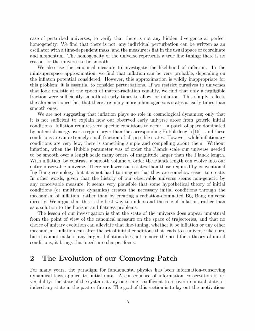
Figure 1: The physical system corresponding to our observable universe. Our comoving patchis defined by the interior of the intersection of our past light cone with a cutoff surface, forexample the surface of last scattering. This illustration is not geometrically faithful, as theexpansion is not linear in time. Despite the change in physical size, we assume that thespace of states is of equal size at every moment.

and isotropic (Robertson-Walker) background spacetime. Defining a particular map from thebackground to our physical spacetime involves a choice of gauge. Nothing that we are goingto do depends on how that gauge is chosen, as long as it is defined consistently throughoutthe history of the universe. Henceforth we assume that we’ve chosen a gauge.

The map from the RW background spacetime to our universe provides two crucial ele-ments: a foliation into time slices, and a congruence of comoving geodesic worldlines. Thetime slicing allows us to think of the universe as a fixed set of degrees of freedom evolvingthrough time, obeying Hamilton’s equations. At each moment in time there exists an exactvalue of the (background) Hubble parameter and all other cosmological parameters.

The notion of comoving worldlines, orthogonal to spacelike hypersurfaces of constantHubble parameter, allows us to define what we mean by our comoving patch. If there is aBig Bang singularity in our past, there is a corresponding particle horizon, defined by theintersection of our past light cone with the singularity. However, independent of the precisenature of the Big Bang, there is an effective limit to our ability to observe the past; inpractice this is provided by the surface of last scattering, although in principle observationsof gravitational waves or other particles could extend the surface backwards. The precisedetails of where we draw the surface aren’t important to our arguments. What matters isthat there exists a well-defined region of three-space interior to the intersection of our pastlight cone with the observability surface past which we can’t see. Our comoving patch, Σ,is simply the physical system defined by the extension of that region forward in time viacomoving worldlines, as shown in Figure 1.

Our assumption is that this comoving patch can be considered as a set of degrees of

7

freedom evolving autonomously through time, free of influence from the rest of the universe.This is clearly an approximation, as an observer stationed close to the boundary of our patchwould see particles pass both into and out of that region; our comoving patch isn’t truly aclosed system. However, the fact that the observable universe is homogenous implies thatthe net effect of that exchange of particles is very small. In particular, we generally don’tbelieve that what happens inside our observable universe depends in any significant way onwhat happens outside.

Note that we are not necessarily assuming that our observable universe is in a pure quan-tum state, free of entanglement with external degrees of freedom; such entanglements don’taffect the local dynamics of the internal degrees of freedom, and therefore are complete com-patible with the von Neumann equation (3). We are, however, assuming that the appropriateHamiltonian is local in space. Holography implies that this is not likely to be strictly true,but it seems like an effective approximation for the universe we observe.

2.2 Unitarity

Autonomy implies that we can consider our comoving patch as a fixed set of degrees offreedom, evolving through time. Our other crucial assumption is that this evolution isunitary (reversible). Even if the underlying fundamental laws of physics are unitary, it isnot completely obvious that the effective evolution of our comoving patch evolves this way.Indeed, this issue is at the heart of the disagreement between those who have emphasizedthe amount of fine-tuning required by inflationary initial conditions [4, 8, 9, 11, 12] and thosewho have argued that they are natural [10, 14].

The issue revolves around the time-dependent nature of the cutoff on modes of a quantumfield in an expanding universe. Since we are working in a comoving patch, there is a naturalinfrared cutoff given by the size of the patch, a length scale of order λIR ∼ aH−1

0 , where a isthe scale factor (normalized to unity today) and H0 is the current Hubble parameter. But

there is also a fixed ultraviolet cutoff at the Planck length, λUV ∼ Lpl =√

8πG. Clearlythe total number of modes that fit in between these two cutoffs increases with time as theuniverse expands. It is therefore tempting to conclude that the space of states is gettinglarger.

We can’t definitively address this question in the absence of a theory of quantum gravity,but for purposes of this paper we will assume that the space of states is not getting larger –which would violate the assumption of unitarity – but the nature of the states is changing.In particular, the subset of states that can usefully be described in terms of quantum fieldson a smooth spacetime background is changing, but those are only a (very small) minorityof all possible states.

The justification for this view comes from the assumed reversibility of the underlyinglaws. Consider the macrostate of our universe today – the set of all microstates compatiblewith the macroscopic configuration we observe. For any given amount of energy density,there are two solutions to the Friedmann equation, one with positive expansion rate andone with negative expansion rate (unless the expansion rate is precisely zero, when thesolution is unique). So there are an equal number of microstates that are similar to our

8

current configuration, except that the universe is contracting rather than expanding. As theuniverse contracts, each of those states must evolve into some unique state a fixed time later;therefore, the number of states accessible to the universe for different values of the Hubbleparameter (or different moments in time) is constant.

Most of the states available when the universe is smaller, however, are not describedby quantum fields on a smooth background. This is reflected in the fact that spatial in-homogeneities would be generically expected to grow, rather than shrink, as the universecontracted. The effect of gravity on the state counting becomes significant, and in particularwe would expect copious production of black holes. These would appear as white holes inthe time-reversed expanding description. Therefore, the overwhelming majority of states atearly times that could evolve into something like our current observable universe are notrelatively smooth spacetimes with gently fluctuating quantum fields; they are expected tobe wildly inhomogeneous, filled with white holes or at least Planck-scale curvatures.

We do not know enough about quantum gravity to explicitly enumerate these states,although some attempts to describe them have been made (see e.g. [16]). But we don’tneed to know how to describe them; the underlying assumption of unitarity implies thatthey are there, whether we can describe them or not. (Similarly, the Bekenstein-Hawkingentropy formula is conventionally taken to imply a large number of states for macroscopicblack holes, even if there is no general description for what those individual states are.)

This argument is not new, and it is often stated in terms of the entropy of our comovingpatch [4, 12]. In the current universe, this entropy is dominated by black holes, and hasa value of order SΣ(t0) ∼ 10104 [17]. If all the matter were part of a single black hole itwould be as large as SΣ(BH) ∼ 10122. At early times, when inhomogeneities were small andlocal gravitational effects were negligible, the entropy was of order SΣ(RD) ∼ 1088. If weassume that the entropy is the logarithm of the number of macroscopically indistinguishablemicrostates, and that every microstate within the current macrostate corresponds to a uniquepredecessor at earlier times, it is clear that the vast majority of states from which ourpresent universe might have evolved don’t look anything like the smooth radiation-dominatedconfiguration we actually believe existed (since exp[10104] exp[1088]).

This distinction between the number of states implied by the assumption of unitarityand the number of states that could reasonably be described by quantum fields on a smoothbackground is absolutely crucial for the question of how finely-tuned are the conditionsnecessary to begin inflation. If we were to start with a configuration of small size and veryhigh density, and consider only those states described by field theory, we would dramaticallyundercount the total number of states. Unitarity could possibly be violated in an ultimatetheory, but we will accept it for the remainder of this paper.

3 The Canonical Measure

In order to quantify the issue of fine-tuning in the context of unitary evolution, we reviewthe canonical measure on the space of trajectories, as examined by Gibbons, Hawking, andStewart [5]. Despite subtleties associated with coordinate invariance, GR can be cast asa conventional Hamiltonian system, with an infinite-dimensional phase space and a set of

9

constraints. The state of a classical system is described by a point γ in a phase space Γ,with canonical coordinates qi and momenta pi. The index i goes from 1 to n, so that phasespace is 2n-dimensional. The classical equations of motion are Hamilton’s equations (1).Equivalently, evolution is generated by a Hamiltonian phase flow with tangent vector

V =∂H∂pi

∂

∂qi− ∂H∂qi

∂

∂pi. (4)

Phase space is a symplectic manifold, which means that it naturally comes equipped witha symplectic form, which is a closed 2-form on Γ:

ω =n∑i=1

dpi ∧ dqi , dω = 0 . (5)

The existence of the symplectic form provides us with a naturally-defined measure on phasespace,

Ω =(−1)n(n−1)/2

n!ωn . (6)

This is the Liouville measure, a 2n-form on Γ. It corresponds to the usual way of integratingdistributions over regions of phase space,∫

f(γ)Ω =

∫f(qi, pi)d

nqdnp . (7)

The Liouville measure is conserved under Hamiltonian evolution. If we begin with aregion A ⊂ Γ, and it evolves into a region A′, Liouville’s theorem states that∫

A

Ω =

∫A′

Ω . (8)

The infinitesimal version of this result is that the Lie derivative of Ω with respect to thevector field V vanishes,

LV Ω = 0 . (9)

These results can be traced back to the fact that the original symplectic form ω is alsoinvariant under the flow:

LV ω = 0 , (10)

so any form constructed from powers of ω will be invariant.In classical statistical mechanics, the Liouville measure can be used to assign weights

to different distributions on phase space. That is not equivalent to assigning probabilitiesto different sets of states, which requires some additional assumption. However, since theLiouville measure is the only naturally-defined measure on phase space, we often assume thatit is proportional to the probability in the absence of further information; this is essentiallyLaplace’s “Principle of Indifference.” Indeed, in statistical mechanics we typically assumethat microstates are distributed with equal probability with respect to the Liouville measure,consistent with known macroscopic constraints.

10

In cosmology, we don’t typically imagine choosing a random state of the universe, subjectto some constraints. When we consider questions of fine-tuning, however, we are comparingthe real world to what we think a randomly-chosen history of the universe would be like. Theassumption of some sort of measure is absolutely necessary for making sense of cosmologicalfine-tuning arguments; otherwise all we can say is that we live in the universe we see, andno further explanation is needed. (Note that this measure on the space of solutions toEinstein’s equation is conceptually distinct from a measure on observers in a multiverse,which is sometimes used to calculate expectation values for cosmological parameters basedon the anthropic principle.)

GHS [5] showed how the Liouville measure on phase space could be used to define a uniquemeasure on the space of solutions (see also [6, 7, 13]). In general relativity we impose theHamiltonian constraint, so we can consider the (2n−1)-dimensional constraint hypersurfaceof fixed Hamiltonian,

C = Γ/H = H∗ . (11)

For Robertson-Walker cosmology, the Hamiltonian precisely vanishes for either open or closeduniverses, so we can take H∗ = 0. Then we consider the space of classical trajectories withinthis constraint hypersurface:

M = C/V , (12)

where the quotient by the evolution vector field V means that two points are equivalent ifthey are connected by a classical trajectory. Note that this is well-defined, in the sense thatpoints in C always stay within C, because the Hamiltonian is conserved.

As M is a submanifold of Γ, the measure is constructed by pulling back the symplecticform from Γ to M and raising it to the (n− 1)th power. GHS constructed a useful explicitform by choosing the nth coordinate on phase space to be the time, qn = t, so that theconjugate momentum becomes the Hamiltonian itself, pn = H. The symplectic form is then

ω = ω + dH ∧ dt , (13)

where

ω =n−1∑i=1

dpi ∧ dqi . (14)

The pullback of ω onto C then has precisely the same coordinate expression as (14), andwe will simply refer to this pullback as ω from now on. It is automatically transverse tothe Hamiltonian flow (ω(V ) = 0), and therefore defines a symplectic form on the space oftrajectories M . The associated measure is a (2n− 2)-form,

Θ =(−1)(n−1)(n−2)/2

(n− 1)!ωn−1 . (15)

We will refer to this as the GHS measure; it is the unique measure on the space of trajectoriesthat is positive, independent of arbitrary choices, and respects the appropriate symmetries[5].

11

To evaluate the measure we need to define coordinates on the space of trajectories. We canchoose a hypersurface Σ in phase space that is transverse to the evolution trajectories, anduse the coordinates on phase space restricted to that hypersurface. An important propertyof the GHS measure is that the integral over a region within a hypersurface is independentof which hypersurface we chose, so long as it intersects the same set of trajectories; if S1

and S2 are subsets, respectively, of two transverse hypersurfaces Σ1 and Σ2 in C, with theproperty that the set of trajectories passing through S1 is the same as that passing throughS2, then ∫

S1

Θ =

∫S2

Θ . (16)

The property that the measure on trajectories is local in phase space has a crucial im-plication for studies of cosmological fine-tuning. Imagine that we specify a certain set oftrajectories by their macroscopic properties today – cosmological solutions that are approx-imately homogeneous, isotropic, and spatially flat, suitably specified in terms of canonicalcoordinates and momenta. It is immediately clear that the measure on this set is indepen-dent of the behavior in very different regions of phase space, e.g. for high-density statescorresponding to early times. Therefore, no choice of early-universe Hamiltonian can makethe current universe more or less finely tuned. No new early-universe phenomena can changethe measure on a set of universes specified at late times, because we can always evaluate themeasure on a late-time hypersurface without reference to the behavior of the universe at anyearlier time.2 At heart, this is a direct consequence of Liouville’s theorem.

4 Minisuperspace

In this section, we evaluate the measure on the space of solutions to Einstein’s equation inminisuperspace (Robertson-Walker) cosmology with a scalar field, applying the results tothe flatness problem and the likelihood of inflation. We will look at two specific models:a scalar with a canonical kinetic term and a potential, and a scalar with a non-canonicalkinetic term chosen to mimic a perfect-fluid equation of state.

A scalar field coupled to general relativity is governed by an action

S =

∫d4x√−g[

1

2R + P (X,φ)

], (17)

where R is the curvature scalar and P is the Lagrange density of the scalar field φ. We haveset m−2

pl = 8πG = 1 for convenience. The scalar Lagrangian is taken to be a function of thefield value and and the kinetic scalar X, defined by

X ≡ −1

2gµν∇µφ∇νφ. (18)

2On the other hand, if the effective Hamiltonian is time-dependent, what looks like a generic state atearly times can evolve into a non-generic state at later times, as energy can be injected into the system. Thisis related to the recent proposal of weak gravity in the early universe [18].

12

We will consider homogeneous scalar fields φ(t) defined in a Robertson-Walker metric,

ds2 = −N2dt2 + a2(t)

[dr2

1− kr2+ r2dΩ2

], (19)

where the spatial curvature parameter k can be normalized to −1, 0, or +1 (so that a(t0) isnot normalized to unity). N is the lapse function, which acts as a Lagrange multiplier. Wethen have

X =1

2N−2φ2. (20)

4.1 Canonical scalar field

We start with the canonical case,

P (X,φ) = X − V (φ). (21)

The Lagrangian for the combined gravity-scalar system in minisuperspace is

L = −3N−1aa2 + 3Nak +1

2N−1a3φ2 −Na3V (φ) . (22)

The canonical coordinates can be taken to be the lapse function N , the scale factor a, andthe scalar field φ. The conjugate momenta are given by pi = ∂L/∂qi, implying

pN = 0 , pa = −6N−1aa , pφ = N−1a3φ . (23)

The vanishing of pN reflects the fact that the lapse function is a non-dynamical Lagrangemultiplier. We can do a Legendre transformation to calculate the Hamiltonian, obtaining

H =∑

piqi − L(pi, q

i) (24)

= N

(− p2

a

12a+

p2φ

2a3+ a3V (φ)− 3ak

). (25)

Varying with respect to N gives the Hamiltonian constraint, H = 0, which is just theFriedmann equation,

H2 =1

3

(1

2φ2 + V (φ)− 3k

a2

). (26)

Henceforth we will set N = 1 (consistent with the equations of motion), leaving us witha four-dimensional phase space,

Γ = φ, pφ, a, pa . (27)

The GHS measure on the space of trajectories is just the the Liouville measure subject tothe constraint that H = 0,

Θ = (dpa ∧ da+ dpφ ∧ dφ)|H=0. (28)

13

Note that the measure in this example is a two-form; the full phase space is four-dimensional,the Hamiltonian constraint surface is three dimensional, so the space of trajectories is two-dimensional.

To express the measure in a convenient form, we use the Friedmann equation to eliminateone of the phase-space variables. Solving for pφ gives us

pφ =

[1

6a2p2

a − 2a6V (φ) + 6a4k

]1/2

. (29)

We can change variables from pa to H using pa = −6a2H, so that

pφ =(6a6H2 − 2a6V + 6a4k

)1/2. (30)

Our coordinates on the constraint hypersurface C are therefore φ, a,H. The basis one-forms appearing in (28) are

dpa = −12aHda− 6a2dH (31)

and

dpφ =6a4HdH − a4V ′dφ+ 6a(3a2H2 − a2V + 2k)da

(6a2H2 − 2a2V + 6k)1/2, (32)

where V ′(φ) = dV/dφ. Plug into the expression (28) for the measure, whose componentsbecome

ΘφH = − 6a4

(6a2H2 − 2a2V + 6k)1/2

ΘHa = −6a2

Θaφ = 63a3H2 − a3V + 2ak

(6a2H2 − 2a2V + 6k)1/2. (33)

The measure is calculated by choosing some transverse surface Σ in phase space, andintegrating Θ over a subset of that surface. If we choose coordinates such that one coordinateis constant over Σ, we simply integrate the orthogonal component of Θ with respect to theother coordinates. One possible choice of the surface Σ is to fix the Hubble parameter,

Σ : H = H∗ . (34)

Any consistent definition is equally legitimate; however, this choice corresponds to our infor-mal idea that initial conditions are set in the early universe when the Hubble parameter isnear the Planck scale. The measure evaluated on a surface of constant H is then the integralof Θaφ,

µ = −6

∫H=H∗

3a3H2∗ − a3V + 2ak

(6a2H2∗ − 2a2V + 6k)1/2

dadφ, (35)

where the minus sign indicates that we have chosen an orientation that will give us a positivefinal answer. We can make this expression look more physically transparent by introducingvariables

Ωφ ≡φ2

6H2∗, ΩV ≡

V (φ)

3H2∗, Ωk ≡ −

k

a2H2∗, (36)

14

so that the Friedmann equation is equivalent to

Ωφ + ΩV + Ωk = 1. (37)

The scale factor is strictly positive, so that integrating over all values of Ωk is equivalent tointegrating over all values of a. Note that −k/Ωk = 1/|Ωk|. We therefore have

da = − 1

2H∗|Ωk|3/2dΩk, (38)

and the measure becomes

µ = 3

√3

2H−2∗

∫H=H∗

1− ΩV − 23Ωk

|Ωk|5/2 (1− ΩV − Ωk)1/2

dΩkdφ (39)

= 3

√3

2H−2∗

∫H=H∗

Ωφ − 13Ωk

|Ωk|5/2Ω1/2

φ

dΩkdφ, (40)

where Ωφ(φ,Ωk) is defined by (37).This integral is divergent. One divergence clearly occurs for small values of the curvature

parameter, Ωk → 0, as the denominator includes a factor of |Ωk|5/2. The integrand alsoblows up at Ωφ = 0 (or equivalently at ΩV + Ωk = 1), but the integral in that region remainsfinite. The integral would also diverge if Ωk or Ωφ were allowed to become arbitrarily large,but that could be controlled by only integrating over a finite range for those quantities, e.g.under the theory that Planckian energy densities or curvatures should not be included inthis classical description.

The important divergence, therefore, is the one at Ωk → 0, i.e. for flat universes. Wediscuss the implications of this divergence in Section 4.3.

4.2 Scalar perfect fluid

In conventional Big Bang cosmology, we generally consider perfect-fluid sources of energysuch as matter or radiation, rather than using a single scalar field. This situation is slightlymore difficult to analyze as a problem in phase space, as homogeneity and isotropy are onlyrecovered after averaging over many individual particles. However, we can model a perfectfluid with an (almost) arbitrary equation of state by a scalar field with a non-canonicalkinetic term [19].

Consider the action (17), where the scalar Lagrangian takes the form P (X,φ), whereX = −(∇µφ)2/2. In a Robertson-Walker background, the energy-momentum tensor takesthe form of a perfect fluid,

Tµν = (ρ+ P )UµUν − Pgµν , (41)

where the pressure is equal to the scalar Lagrange density itself (thereby accounting for thechoice of notation). The fluid has four-velocity

Uµ = (2X)−1/2∇µφ (42)

15

and energy densityρ = 2X∂XP − P. (43)

We will be interested in a vanishing potential but a non-canonical kinetic term,

P (X,φ) =2n−1

nXn =

1

2nN−2nφ2n. (44)

This gives a fluid with a density

ρ =2n− 1

2nN−2nφ2n, (45)

corresponding to a constant equation-of-state parameter

w = P/ρ =1

2n− 1, (46)

as can easily be checked. Therefore we can model the behavior of radiation (w = 1/3) bychoosing n = 2, and approximate matter (w = 0) by choosing n very large.

The scalar-Einstein Lagrangian in a Robertson-Walker background takes the form

L = −3N−1aa2 + 3Nak +1

2nN−(2n−1)a3φ2n, (47)

and the Friedmann equation is

H2 ≡(a

a

)2

=

(2n− 1

6n

)φ2n − k

a2, (48)

where we have set N = 1. We can duplicate the steps taken in the previous section, toevaluate the GHS measure in terms of coordinates φ, a,H. We end up with

ΘφH = −(

2n− 1

2n

)1/2n6a6n/(2n−1)

[a6n/(2n−1)3H2 + 3a2(n+1)/(2n−1)k]1/2n

ΘHa = −6a2

Θaφ = 6(2n− 1)(1−2n)/2n na(4n+1)/(2n−1)3H2 + (n+ 1)a3/(2n−1)k

[2na6n/(2n−1)3H2 + 6na2(n+1)/(2n−1)k]1/2n

. (49)

To calculate the measure of a set of trajectories over a surface of constant H = H∗, weintegrate Θaφ over a and φ. This yields

µ = −3

(2n− 1

6n

)(1−2n)/2n ∫H=H∗

a2 H2∗ + (n+1)

3na−2k

(H2∗ + a−2k)1/2n

dadφ. (50)

Note that the integrand has no dependence on φ, since there was no potential in the originalaction. We therefore define

x ≡ 3

(2n− 1

6n

)(1−2n)/2n ∫dφ, (51)

16

which contributes an overall multiplicative constant to the measure. As before, it is conve-nient to change variables from a to Ωk = −k/a2H2

∗ . This leaves us with

µ =x

2H(n+1)/n∗

∫1− (n+1)

3nΩk

|Ωk|5/2 (1− Ωk)1/2n

dΩk. (52)

This will diverge for small Ωk for any value of n; all of the measure is at spatially flatuniverses. This of course includes the case of radiation, n = 2. Therefore, the divergence wefound in the previous subsection for flat universes does not seem to depend on the details ofthe matter action.

4.3 The flatness problem

Let’s return to the expression for the measure (40) we derived for Robertson-Walker universeswith a scalar field featuring a canonical kinetic term and a potential,

µ ∝∫H=H∗

1− ΩV − 23Ωk

|Ωk|5/2 (1− ΩV − Ωk)1/2

dΩkdφ. (53)

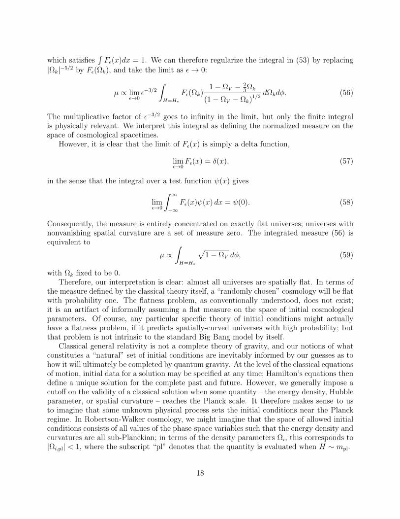
We have left out the numerical constants in front, as the overall normalization is irrelevant.It is clear that this is non-normalizable as it stands; the integral diverges near Ωk = 0,which is certainly a physically allowed region of parameter space. This non-normalizabilityis problematic if we would like to interpret the measure as determining the relative fractionof universes with different physical properties.

We propose that the proper way of handling such a divergence is to regularize it. Thatis, we define a series of integrals that are individually finite, and which approach the originalexpression as the regulator parameter ε is taken to zero. We can then isolate an appropriatepower of ε by which we can divide the regulated expression, so that we isolate the finite partof the result as ε goes to zero.

The divergence in (53) can be regulated by “smoothing” the factor |Ωk|−5/2 in an ε-neighborhood around Ωk = 0 to get a finite integral. Consider the function

fε(x) =

|x|−5/2 if |x| ≥ ε,

ε−5/2 if |x| < ε.(54)

Clearly limε→0 fε(x) = |x|−5/2, our original function. The integral of fε(x) over all values ofx is 10

3ε−3/2. So we obtain a normalized integral by introducing the function

Fε(x) =

3ε3/2

10|x|5/2if |x| ≥ ε,

3

10εif |x| < ε,

(55)

17

which satisfies∫Fε(x)dx = 1. We can therefore regularize the integral in (53) by replacing

|Ωk|−5/2 by Fε(Ωk), and take the limit as ε→ 0:

µ ∝ limε→0

ε−3/2

∫H=H∗

Fε(Ωk)1− ΩV − 2

3Ωk

(1− ΩV − Ωk)1/2

dΩkdφ. (56)

The multiplicative factor of ε−3/2 goes to infinity in the limit, but only the finite integralis physically relevant. We interpret this integral as defining the normalized measure on thespace of cosmological spacetimes.

However, it is clear that the limit of Fε(x) is simply a delta function,

limε→0

Fε(x) = δ(x), (57)

in the sense that the integral over a test function ψ(x) gives

limε→0

∫ ∞−∞

Fε(x)ψ(x) dx = ψ(0). (58)

Consequently, the measure is entirely concentrated on exactly flat universes; universes withnonvanishing spatial curvature are a set of measure zero. The integrated measure (56) isequivalent to

µ ∝∫H=H∗

√1− ΩV dφ, (59)

with Ωk fixed to be 0.Therefore, our interpretation is clear: almost all universes are spatially flat. In terms of

the measure defined by the classical theory itself, a “randomly chosen” cosmology will be flatwith probability one. The flatness problem, as conventionally understood, does not exist;it is an artifact of informally assuming a flat measure on the space of initial cosmologicalparameters. Of course, any particular specific theory of initial conditions might actuallyhave a flatness problem, if it predicts spatially-curved universes with high probability; butthat problem is not intrinsic to the standard Big Bang model by itself.

Classical general relativity is not a complete theory of gravity, and our notions of whatconstitutes a “natural” set of initial conditions are inevitably informed by our guesses as tohow it will ultimately be completed by quantum gravity. At the level of the classical equationsof motion, initial data for a solution may be specified at any time; Hamilton’s equations thendefine a unique solution for the complete past and future. However, we generally impose acutoff on the validity of a classical solution when some quantity – the energy density, Hubbleparameter, or spatial curvature – reaches the Planck scale. It therefore makes sense to usto imagine that some unknown physical process sets the initial conditions near the Planckregime. In Robertson-Walker cosmology, we might imagine that the space of allowed initialconditions consists of all values of the phase-space variables such that the energy density andcurvatures are all sub-Planckian; in terms of the density parameters Ωi, this corresponds to|Ωi,pl| < 1, where the subscript “pl” denotes that the quantity is evaluated when H ∼ mpl.

18

-1.0 -0.5 0.0 0.5 1.0Wk

1

2

3

4

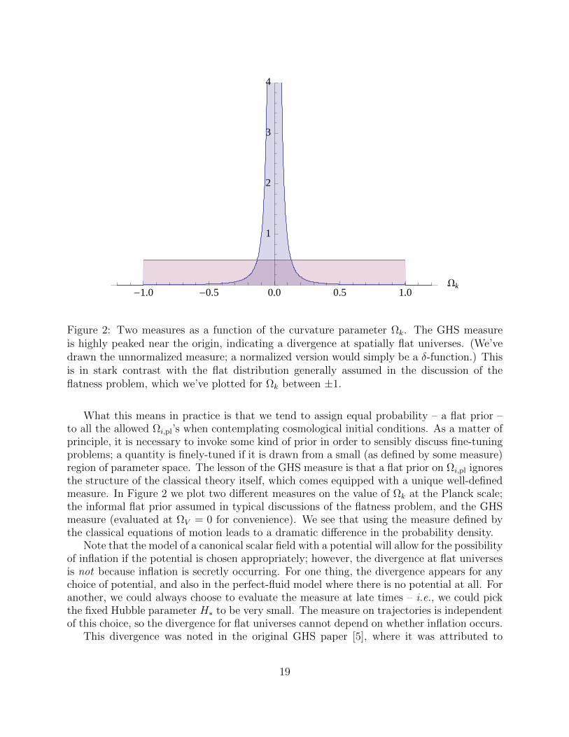
Figure 2: Two measures as a function of the curvature parameter Ωk. The GHS measureis highly peaked near the origin, indicating a divergence at spatially flat universes. (We’vedrawn the unnormalized measure; a normalized version would simply be a δ-function.) Thisis in stark contrast with the flat distribution generally assumed in the discussion of theflatness problem, which we’ve plotted for Ωk between ±1.

What this means in practice is that we tend to assign equal probability – a flat prior –to all the allowed Ωi,pl’s when contemplating cosmological initial conditions. As a matter ofprinciple, it is necessary to invoke some kind of prior in order to sensibly discuss fine-tuningproblems; a quantity is finely-tuned if it is drawn from a small (as defined by some measure)region of parameter space. The lesson of the GHS measure is that a flat prior on Ωi,pl ignoresthe structure of the classical theory itself, which comes equipped with a unique well-definedmeasure. In Figure 2 we plot two different measures on the value of Ωk at the Planck scale;the informal flat prior assumed in typical discussions of the flatness problem, and the GHSmeasure (evaluated at ΩV = 0 for convenience). We see that using the measure defined bythe classical equations of motion leads to a dramatic difference in the probability density.

Note that the model of a canonical scalar field with a potential will allow for the possibilityof inflation if the potential is chosen appropriately; however, the divergence at flat universesis not because inflation is secretly occurring. For one thing, the divergence appears for anychoice of potential, and also in the perfect-fluid model where there is no potential at all. Foranother, we could always choose to evaluate the measure at late times – i.e., we could pickthe fixed Hubble parameter H∗ to be very small. The measure on trajectories is independentof this choice, so the divergence for flat universes cannot depend on whether inflation occurs.

This divergence was noted in the original GHS paper [5], where it was attributed to

19

“universes with very large scale factors” due to a different choice of variables. This isnot the most physically transparent characterization, as any open universe will eventuallyhave a large scale factor. It is also discussed by Gibbons and Turok [13], who correctlyattribute it to nearly-flat universes. However, they advocate discarding all such universesas physically indistinguishable, and concentrating on the non-flat universes. To us, thisseems to be throwing away almost all the solutions, and keeping a set of measure zero. It istrue that universes with almost identical values of the curvature parameter will be physicallyindistinguishable, but that doesn’t affect the fact that almost all universes have this property.In Hawking and Page [6] and Coule [7] the divergence is directly attributed to flat universes,but they do not seem to argue that the flatness problem is therefore an illusion.

The real world is not precisely Robertson-Walker, so in some sense the flatness problemis not rigorously defined; a super-Hubble-radius perturbation could lead to a deviation fromΩ = 1 in our observed universe, even if the background cosmology were spatially flat. Nev-ertheless, the unanticipated structure of the canonical measure in minisuperspace serves asa cautionary example for the importance of considering the space of initial conditions in arigorous way. More directly, it raises an obvious question: if the canonical measure is concen-trated on spatially flat universes, might it also be concentrated on smooth universes, therebycalling into question the status of the horizon problem as well as the flatness problem? (Wewill find that it is not.)

4.4 Likelihood of inflation

A common use of the canonical measure has been to calculate the likelihood of inflation[5, 6, 7]. Most recently, Gibbons and Turok [13] have argued that the fraction of universesthat inflate is extremely small. However, they threw away all but a set of measure zero oftrajectories, on the grounds that they all had negligibly small spatial curvature and thereforephysically indistinguishable. Inflation, of course, tends to make the universe spatially flat,so this procedure is potentially unfair to the likelihood of inflation. We therefore re-examinethis question, following the philosophy suggested by the above analysis, which implies thatalmost all universes are spatially flat. We choose to look only at flat universes, and calculatethe fraction that experience more than sixty e-folds of inflation. We will look at two choicesof potential: a massive scalar, and a pseudo-Goldstone boson. (We will argue in the nextsection that these results are physically irrelevant, as perturbations play a crucial role.)

We start with a massive scalar field with mφ = 3 × 10−3mpl, which yields an amplitudeof perturbations that agrees with observations. We choose to evaluate the measure on thehypersurface H = 1/

√3, so that the Friedmann equation becomes 1 = 1

2φ2 + 1

2m2φ2. After

replacing the divergence at zero curvature in (52) by a delta function, the normalized measurebecomes

µ =

√2m

π

∫H=1/

√3

√1− 1

2m2φ2 dφ. (60)

(Recall that we have set mpl = 1/√

8πG = 1.) The range of integration is |φ| ≤√

2/m2φ (or

ρφ ≤ 1), corresponding to V ≤ 1.

20

We used the Euler method with a time step ∆t = 10−3 to numerically follow the evolutionof the scale factor and the scalar field. We find that the universe undergoes more than sixty e-folds of inflation for all initial values of φ except for the range −24 to 6 if φ > 0 (for φ < 0, therange would be −6 to 24 due to the symmetry of the potential). For simplicity, we disregardin our calculation the expansion that occurs after the first period of slow-roll inflation. (Weverified numerically that subsequent periods of slow-roll expansion are relatively brief andlead to very little further expansion.) Excluding the region −24 ≤ φ ≤ 6, the measure (60)integrates to 0.99996. It seems highly likely to have more than sixty e-folds of inflation bythis standard.

As another example we consider inflation driven by a pseudo-Goldstone boson [20] withpotential

V (φ) = Λ4(1 + cos(φ/f)). (61)

In our calculation, we use f =√

8π and Λ = 10−3, so that the model is consistent withWMAP3 data [21]. We evaluate the measure on the hypersurface H = H∗ =

√4/3Λ2, so

that 3H2∗ = 2Vmax = 4Λ4. In this case, the normalized measure becomes

µ =1

8√πE[−1]

∫H∗=√

4/3Λ2

√1− 1

4

(1 + cos

φ√8π

)dφ, (62)

where E[m] is the elliptic integral∫ 2π

0

√1−m sin2 tdt. Numerically we find that the universe

expands by more than 60 efolds for −4.0 < φ < 2.4 if φ > 0 at H = H∗ =√

4/3Λ2. (Theevenness of the potential allows us to consider only this branch of solutions.) Evaluating themeasure gives a probability of 0.171. Notice that this is not too different from the calculationin [20], which gives 0.2 by assuming that φ is randomly distributed between 0 and

√8π. We

also note that the probability is rather sensitive to the value of f ; numerical evidence suggestthat it increases with f (a flatter potential).

Both of these examples lead to the conclusion that inflation has a very reasonable chanceof occurring. Indeed, it is sometimes claimed that inflation is an “attractor” (see e.g. [24]),but that is a misleading abuse of nomenclature. It is a basic feature of dynamical systemstheory that there are no attractors in true Hamiltonian mechanics; Liouville’s theorem im-plies that the total volume of a region of phase space remains constant under time evolution.Attractors, in the rigorous sense of the word, only occur for systems with dissipation. In-flation appears to be an attractor only because it is often convenient to portray “phaseportraits” in terms of the inflaton φ and its time derivative, φ. But φ is not the momentumconjugate to φ; as seen in (23), with the lapse function set to N = 1, it is pφ = a3φ. Tra-

jectories drawn on a (φ, φ) plot tend to approach a fixed point, but only because the scalefactor a is dramatically increasing, not because of any true attractor behavior.

These calculations of the likelihood of inflation are of dubious physical relevance. Exam-ining a single scalar field in minisuperspace is an extremely unrealistic scenario. At a verysimple level, if there are other massless fields in the problem, any of them may share someof the energy density, reducing the probability that the inflaton potential dominates. Moreimportantly, the role of perturbations is crucial. The real reason why inflation is unlikely

21

from the point of view of the canonical measure is not because it is unlikely in minisuper-space, but because perturbations can easily be sufficiently large to prevent inflation fromever occurring. We examine this issue in detail in the next section.

5 Perturbations

The horizon problem is usually formulated in terms of the absence of causal contact betweenwidely-separated points in the early universe. Operationally, however, it comes down to thefact that the universe is smooth over large scales. We can investigate the measure associatedwith such universes by looking at perturbed Robertson-Walker cosmologies. While the set ofall perturbations defines a large-dimensional phase space, in linear perturbation theory wecan keep things simple by looking at a single mode at a time. We will find that, in contrastwith the surprising result of the last section, the measure on perturbations is just what wewould expect – there is no divergence at nearly-smooth universes. However, this implies thatonly an imperceptibly small fraction of spacetimes were sufficiently smooth at early times toallow for inflation to occur.

To calculate the measure for scalar perturbations, we need to first compute the corre-sponding action. We are interested in universes dominated by hydrodynamical matter suchas dust or radiation. For linear scalar perturbations, the coupled gravity-matter system canbe described by a single independent degree of freedom, as discussed by Mukhanov, Feld-man and Brandenberger [22]; we will follow closely the discussion in [23]. After obtainingthe action, we can isolate the dynamical variables and construct the symplectic two-formon phase space, which can then be used to compute the measure on the set of solutionsto Einstein’s equations. A slight subtlety arises because the corresponding Hamiltonian istime-dependent, but this is easily dealt with.

5.1 Description of perturbations

In this section it will be convenient to switch to conformal time,

η =

∫a−1dt. (63)

Derivatives with respect to η are denoted by the superscript ′, and H ≡ a′/a is related to

the Hubble parameter H = a/a by H = aH. The Friedmann equations become

H2 =8πG

3a2ρ− k, (64)

H ′ = −4πG

3a2(ρ+ 3p), (65)

where ρ and p are the background density and pressure. In a flat universe with only matterand radiation, in the radiation-dominated era we have

η(RD) =a

H0√aeq

, H(RD) = η−1, (66)

22

where aeq is the scale factor at matter-radiation equality, and now we set the current scalefactor to unity, a0 = 1. Numerically, the conformal time in the radiation-dominated era isapproximately

η(T ) ≈ 5× 1030

T (eV)eV−1. (67)

The metric for a flat RW universe in conformal time with scalar perturbations is

ds2 = a2(η)[−(1 + 2Φ)dη2 + 2B,idηdx

2 + ((1− 2Ψ)δij + 2E,ij)dxidxj

], (68)

where Φ, Ψ, E, and B are scalar functions characterizing metric perturbations, and commasdenote partial derivatives. It is useful to define the gauge-invariant Newtonian potential,

Φ = φ− 1

a[a(B − E)′]

′, (69)

and the gauge-invariant energy-density perturbation,

δρ = δρ− ρ′(B − E ′). (70)

For scalar perturbations in the absence of anisotropic stress, these are related by

δρ =1

4πGa2

[∇2Φ− 3H(Φ′ + HΦ)

]. (71)

For adiabatic perturbations (δS = 0), the potential obeys an autonomous equation,

Φ′′ + 3(1 + c2s)HΦ′ − c2

s∇2Φ + [2H ′ + (1 + 3c2s)H

2]Φ = 0, (72)

where c2s = ∂p/∂ρ is the speed of sound squared in the fluid. This equation simplifies if we

introduce the rescaled perturbation variable

u ≡ Φ√ρ+ p

, (73)

and the time-dependent parameter

θ = exp

[3

2

∫(1 + c2

s)Hdη

]Φ =

1

a

[2

3

(1− H ′

H2

)]−1/2

. (74)

In terms of these (72) becomes

u′′ − c2s∇2u− θ′′

θu = 0. (75)

The variable u is a single degree of freedom that encodes both the gravitational potential[through (73)] and the density perturbation [through (71)]. The equation of motion (75)corresponds to an action

Su =1

2

∫d4x

(u′2 − c2

su,iu,i +θ′′

θu2

). (76)

23

Defining the conjugate momentum pu = ∂L/∂u′ = u′, we can describe the dynamics in termsof a Hamiltonian density for an individual mode with wavenumber k,

H =1

2p2u +

1

2

(c2sk

2 − θ′′

θ

)u2. (77)

This is simply the Hamiltonian for a single degree of freedom with a time-dependent effectivemass m2 = c2

sk2 − θ′′/θ.

5.2 Computation of the measure

Given the Hamiltonian (77), we can straightforwardly compute the invariant measure onphase space. One caveat is that now the Hamiltonian is time-dependent, because the effectivemass evolves. The carrier manifold of the Hamiltonian therefore has an odd number ofdimensions. We can retain the symplecticity of a time-dependent Hamiltonian system (whichrequires an even number of dimensions) by promoting time to be an addition canonicalcoordinate, qn+1 = t. The conjugate momentum is minus the Hamiltonian, pn+1 = −H. Wecan then define an extended Hamiltonian by

H+ = H(p, q, t) + pn+1. (78)

This is formally time-independent, and recovers the original Hamiltonian equations via

qi =∂H+

∂pi, pi = −∂H+

∂qi, (79)

along with two additional trivial equations t = 1 and H = ∂H/∂t.With t promoted to a coordinate, the time-dependent Hamiltonian system also comes

equipped naturally with a closed symplectic two-form, now with an additional term:

ω =n∑i=1

dpi ∧ dqi − dH ∧ dt. (80)

The invariance of the form of Hamilton’s equations ensures that the Lie derivative of ω withrespect to the vector field generated by H+ vanishes. The top exterior power of ω is thenguaranteed to be conserved under the extended Hamiltonian flow, and can thus play the roleof the Liouville measure for the augmented system. The GHS measure can then be obtainedby pulling back the Liouville measure onto a hypersurface intersecting the trajectories andsatisfying the constraint H+ = 0.

In our case, the original system, with coordinate u and conjugate momentum pu, isaugmented to one with two coordinates u and η and their conjugate momenta pu and −H.The extended Hamiltonian,

H+ =1

2p2u +

1

2

(c2sk

2 − θ′′

θ

)u2 −H, (81)

24

is time-independent and set to zero by the equations of motion. Its conservation is analogousto the Friedmann equation constraint in the analysis of the flatness problem. Using (80),the GHS measure Θ for the perturbations is the two-form

Θ = dpu ∧ du− (dH ∧ dη)|H+=0

= dpu ∧ du−1

2d

[p2u +

(c2sk

2 − θ′′

θ

)u2

]∧ dη

= dpu ∧ du− pu(dpu ∧ dη)− u(c2sk

2 − θ′′

θ

)du ∧ dη . (82)

One convenient hypersurface in which we can evaluate the flux of trajectories is η =η∗ = constant. (This is equivalent to a surface of H = constant or a = constant, althoughthose are not coordinates in the phase space of the perturbation.) As η is always positive ina matter- and radiation-dominated universe, this surface intersects all trajectories exactlyonce. We then have

µ =

∫η=η∗

Θpuududpu

=

∫η=η∗

dudpu. (83)

The flux of trajectories crossing this surface is unity, implying that all values for u and pu areequally likely. There is nothing in the measure that would explain the small observed valuesof perturbations at early times. Hence, the observed homogeneity of our universe does implyconsiderable fine-tuning; unlike the flatness problem, the horizon problem is real.

5.3 Likelihood of inflation

We can use the canonical measure on perturbations to estimate the likelihood of inflation.Our strategy will be to consider universes dominated by matter and radiation – i.e., thesupposed post-inflationary era in the universe’s history – and ask what fraction of themcould have begun with inflation. This is somewhat contrary to the conventional approach,which might start with an assumed early state of the universe and ask whether inflation willbegin; but it is fully consistent with the philosophy of unitary and autonomous evolution,and takes advantage of the feature of the canonical measure that it can be evaluated at anytime.

If inflation does occur, perturbations will be very small when it ends. Indeed, pertur-bations must be sub-dominant if inflation is to begin in the first place [15], and by the endof inflation only small quantum fluctuations in the energy density remain. It is thereforea necessary (although not sufficient) condition for inflation to occur that perturbations besmall at early times. For convenience, we will take inflation to end near the GUT scale,TG = 1016 GeV (ηG ≈ 6× 105 eV−1), although this choice is not crucial.

We therefore want to calculate what fraction of perturbed Robertson-Walker universesare relatively smooth near the GUT scale. We take “smooth” to mean that both the density

25

contrast δ = δρ/ρ and the Newtonian potential Φ are less than one. Because the phase spaceis unbounded and the measure (83) is flat, it is necessary to cut off the space of perturbationsin some way. We might define “realistic” cosmologies as those that match the homogeneityof our observed universe at the redshift of recombination z ∼ 1200, when CMB temperatureanisotropies are observed. Our expressions will be much less cumbersome, however, if wedemand smoothness at matter-radiation equality, zeq ∼ 3000 (ηeq ≈ 1031 eV−1), within anorder of magnitude of recombination. Since the observed temperature anisotropies are oforder one part in 105, we therefore define a realistic universe as one with δeq ≤ 10−5 andΦeq ≤ 10−5.

There is a long-distance cutoff on the modes we consider given by the size of our comovingobservable universe, extrapolated back to matter-radiation equality. The size L0 of ourobservable universe today is a few times H−1

0 = 1033 eV−1, and the size of our comovingpatch at equality is aeq = 1/3000 times that, so

Leq ≈ 1030 eV−1. (84)

We will also impose a short-distance cutoff at the Hubble radius at equality,

H−1eq ≈ mpl

(a2

eq

T 20

)≈ 1028 eV−1. (85)

The total number of modes we consider is therefore

n =

(Leq

H−1eq

)3

≈ 106. (86)

Our short-distance cutoff is chosen primarily for convenience; there is a natural ultravioletcutoff set by the scale below which the hydrodynamical approximation becomes invalid, butthat is much shorter than H−1

eq . It is clear that we are neglecting a large number of modesthat could plausibly have large amplitudes at early times; our result will therefore represent agenerous overestimate of the fraction of inflationary spacetimes. The final numerical answerwill be small enough that this shortcut won’t matter.

With this setup in place, we would like to compare the measure on trajectories that aresmooth near the GUT scale to the measure on those that are realistic near matter-radiationequality. We therefore only need to consider a single kind of evolution – long-wavelengthmodes (super-Hubble-radius, cskη < 1) in a radiation-dominated universe. In that case thegeneral solution to our evolution equation (75) is

u = c1θ + c2θ

∫η0

θ−2 dη, (87)

where c1 and c2 are constants. During radiation domination we have

θ =

√3

2√aeqH0

η−1. (88)

26

The solution for u is thereforeu = αη−1 + βη2, (89)

where α and β are constants. The conjugate momentum is

pu = −αη−2 + 2βη. (90)

The potential is related to u by (73). In the radiation era we have

(ρ+ p)1/2 = γη−2, (91)

where we have defined

γ =2mpl√aeqH0

. (92)

Our general solution is therefore

Φ = γ(αη−3 + β). (93)

Finally we turn to the density perturbation, which is given by (71). The ∇2Φ = −k2Φ termis negligible for long wavelengths, so we’re left with

δρ =12m3

pl

a3/2eq H3

0

(2αη−7 − βη−4), (94)

which in turn implies

δ ≡ δρ

ρ= 2γ(2αη−3 − β). (95)

To calculate the measure, it is convenient to use α and β as the independent variablesthat specify a mode. The measure is simply

µ =

∫dudpu = 3

∫dαdβ. (96)

This comes from taking the derivative of (89) and (90), treating α and β as the independentvariables, and computing du∧dpu. No η-dependent factors appear when we write the measurein terms of α and β. We can also express it in terms of the density contrast and Newtonianpotential,

dΦdδ = 6γ2η−3dαdβ. (97)

Therefore, a region in the Φ-δ plane at time ηG has a measure that is larger than the samecoordinate region at time ηeq by a factor of(

ηeq

ηG

)3

≈ 1076. (98)

27

The coordinate area of our initial region at the GUT scale is ∆ΦG∆δG ≈ 1, while thecoordinate area of our region at equality is ∆Φeq∆δeq ≈ (10−5)2 = 10−10. For each mode,we therefore have

µ(inflationary)

µ(realistic)=

(ηG

ηeq

)3∆ΦG∆δG

∆Φeq∆δeq

≈ 10−66. (99)

This is saying that, for a given wave vector, only 10−66 of the allowed amplitudes that arerealistic at matter-radiation equality are small at the GUT scale. To allow for inflation, werequire that modes of every fixed comoving wavelength and direction be less than unity atthe GUT scale; the fraction of realistic cosmologies that are eligible for inflation is therefore

P (inflation) ≈ (10−66)n ≈ 10−6.6×107 . (100)

This is a small number, indicating that a negligible fraction of universes that are realisticat late times experienced a period of inflation at very early times. We derived this particularvalue by assuming the universe was realistic at matter-radiation equality, but similarly tinyfractions would apply had we started with any other time in the late universe. We also lookedat only a fraction of possible modes, so a more careful estimate would yield a much smallernumber. Indeed, using entropy as a proxy for the number of states yields estimates of order10−10122 [4]. Clearly, the precise numerical answer is not of the essence; the conclusion is thatinflationary trajectories are a negligible fraction of all possible evolutions of the universe.

A crucial feature of this analysis is that we allowed for the possibility of decaying cos-mological perturbations; if all we know about the perturbations is that they are small atmatter-radiation equality, the generic case is that many have been decaying since earliertimes. Such decaying modes are often neglected in cosmology, but for our purposes thatwould be begging the question. A successful theory of cosmological initial conditions willaccount for the absence of such modes, not presume it.

6 Discussion

We have investigated the issue of cosmological fine-tuning under the assumption that ourobservable universe evolves unitarily through time. Using the invariant measure on cosmo-logical solutions to Einstein’s equation, we find that the flatness problem is an illusion; inthe context of purely Robertson-Walker cosmologies, the measure diverges on flat universes.In the case of deviations from homogeneity, however, we recover something closer to theconventional result; in appropriate variables, the measure on the phase space of any partic-ular mode of perturbation is flat, so that a generic universe would be expected to be highlyinhomogeneous.

Inflation by itself cannot solve the horizon problem, in the sense of making the smoothearly universe a natural outcome of a wide variety of initial conditions. The assumptionsof unitarity and autonomy applied to our comoving patch imply that any set of states atlate times necessarily corresponds to an equal number of states at early times. Differentchoices for the Hamiltonian relevant in the early universe cannot serve to focus or spread thetrajectories, which would violate Liouville’s theorem; they can only deflect the trajectories

28

in some overall way. Therefore, whether or not a theory allows for inflation has no impacton the total fraction of initial conditions that lead to a universe that looks like ours at latetimes.

This basic argument has been appreciated for some time; indeed, its essential featureswere outlined by Penrose [4] even before inflation was invented. Nevertheless, it has failedto make an important impact on most discussions of inflationary cosmology. Attitudestoward this line of inquiry fall roughly into three camps: a small camp who believe that theimplications of Liouville’s theorem represent a significant challenge to inflation’s purportedability to address fine-tuning problems [8, 9, 11, 12, 13]; an even smaller camp who explicitlyargue that the allowed space of initial conditions is much smaller than the space of laterconditions, in apparent conflict with the principles of unitary evolution [10, 14]; and a verylarge camp who choose to ignore the issue or keep their opinions to themselves.

But this issue is crucial to understanding the role of inflation (or any alternative mech-anism) in accounting for the apparent fine-tuning of our universe. The part of the universewe observe consists of a certain set of degrees of freedom, arranged in a certain way – a fewhundred billion galaxies, distributed approximately uniformly through an expanding space– and apparently evolving from a very finely-tuned smooth Big-Bang-like beginning. Un-derstanding why things are this way could have crucial consequences for our view of otherfeatures of the universe, much as the inflationary scenario revolutionized our ideas about theorigin of cosmological perturbations.

There seem to be two possible ways we might hope to account for the apparent fine-tuningof the history of the observable universe:

1. The present configuration of the universe only occurs once. In this case, the evolutionfrom the Big Bang to today is highly non-generic, and the question becomes why thisevolution, rather than some other one. The answer might be found in properties of thewave function of the universe (e.g. [25]).

2. Degrees of freedom arrange themselves in configurations like the observable universemany times in the history of a much larger multiverse. In this case, there is stillhope that the overall evolution may be generic, if it can be shown that configurationslike ours most often occur in the aftermath of a smooth Big Bang. The apparentrestrictions of Liouville’s theorem may be circumvented by imagining that the degreesof freedom of our current universe do not describe a closed system for all time, butinteract strongly with other degrees of freedom at some times (e.g. by arising as babyuniverses [12]).

In either case, inflation could play an important role as part of a more comprehensivepicture. While inflation does not make universes like ours more numerous in the space ofall possible universes, it might provide a more reasonable target for a true theory of initialconditions, from quantum cosmology or elsewhere. (This is a possible reading of [10, 14],although those authors seem to exclude non-smooth initial conditions a priori, rather thanrelying on some well-defined theory of initial conditions.)

As we have shown in this paper, most universes that are smooth at matter-radiationequality were wildly inhomogeneous at very early times. But the converse is not true; most

29

universes that were wildly inhomogeneous at early times simply stay that way. The processof smoothing out represents a violation of the Second Law of Thermodynamics, as entropydecreases along the way. Even though the vast majority of trajectories that are smooth atmatter-radiation equality were inhomogeneous at early times, it seems intuitively unlikelythat the real universe behaves this way; much more plausible is the conventional suppositionthat the universe was smoother (and entropy was lower) all the way back to the Big Bang.

One way of expressing why this seems more natural to us is that the corresponding initialstates are very simple to characterize: they are smooth within an appropriate comovingvolume. In contrast, the much more numerous histories that begin inhomogeneously andproceed to smooth out are impossible to characterize in terms of macroscopically observablequantities at early times; the fact that they will ultimately smooth out is hidden in extremelysubtle correlations between a multitude of degrees of freedom.3 It seems much easier toimagine that an ultimate theory of initial conditions will produce states that are simple todescribe rather than ones that feature an enormous number of mysterious and inaccessiblecorrelations. It may be true that a randomly-chosen universe like ours would have begun ina wildly inhomogeneous state; but it’s clear that the history of our observable universe isnot a randomly-chosen evolution of the corresponding degrees of freedom.

Given that we need some theory of initial conditions to explain why our universe wasnot chosen at random, the question becomes whether inflation provides any help to thisunknown theory. There are two ways in which it does. First, inflation allows the initialpatch of spacetime with a Planck-scale Hubble parameter to be physically small, whileconventional cosmology does not. If we extrapoloate a matter- and radiation-dominateduniverse from today backwards in time, a comoving patch of size H−1

0 today corresponds toa physical size ∼ 10−26H0 ∼ 1034Lpl ∼ 1 cm when H = mpl. In contrast, with inflation, thesame patch needs to be no larger than Lpl when H = mpl, as emphasized by Kofman, Linde,and Mukhanov [10, 14]. If our purported theory of initial conditions, whether quantumcosmology or baby-universe nucleation or some other scheme, has an easier time makingsmall patches of space than large ones, inflation would be an enormous help.

The other advantage is in the degree of smoothness required. Without inflation, a perfect-fluid universe with Planckian Hubble parameter would have to be extremely homogeneousto be compatible with the current universe, while an analogous inflationary patch couldaccommodate any amount of sub-Planckian perturbations. While the actual number oftrajectories may be smaller in the case of inflation, there is a sense in which the requirementsseem more natural. Within the set of initial conditions that experience sufficient inflation,all such states give us reasonable universes at late times; in a more conventional Big Bangcosmology, the perturbations require an additional substantial fine tuning. Again, we havea relatively plausible target for a future comprehensive theory of initial conditions: as longas inflation occurs, and the perturbations are not initially super-Planckian, we will get areasonable universe.

3The situation resembles the time-reversal of a glass of water with an ice cube that melts over the courseof an hour. At the end of the melting process, if we reverse the momentum of every molecule in the glass, wewill describe an initial condition that evolves into an ice cube. But there’s no way of knowing that, just fromthe macroscopically available information; the surprising future evolution is hidden in subtle correlationsbetween different molecules.

30

These features of inflation are certainly not novel; it is well-known that inflation allowsfor the creation of a universe such as our own out of a small and relatively small bubbleof false vacuum energy. We are nevertheless presenting the point in such detail because webelieve that the usual sales pitch for inflation is misleading; inflation does offer importantadvantages over conventional Friedmann cosmologies, but not necessarily the ones that areoften advertised. In particular, inflation does not by itself make our current universe morelikely; the number of trajectories that end up looking like our present universe is unaffectedby the possibility of inflation, and even when it is allowed only a tiny minority of solutionsfeature it. Rather, inflation provides a specific kind of set-up for a true theory of initialconditions – one that is yet to be definitively developed.

Acknowledgments

This work was supported in part by the U.S. Dept. of Energy and the Gordon and BettyMoore Foundation. We thank Andy Albrecht, Adrienne Erickcek, Don Page, and PaulSteinhardt for helpful conversations.

7 Appendix: Eternal Inflation

Eternal inflation [26, 27, 28, 29] is sometimes held up as a solution to the puzzle of theunlikeliness of inflation occurring. In many models of inflation, the process is eternal – whilesome regions reheat and become radiation-dominated, other regions (increasing in physicalvolume) continue to inflate. This may be driven by the back-reaction of large quantumfluctuations in the inflaton during slow-roll inflation, or simply by the failure of percolationin a false vacuum with a sufficiently small decay rate.

Through eternal inflation, a small initially inflating volume grows without bound, creatingan ever-increasing number of pocket universes that expand and cool in accordance withconventional cosmology. Therefore, the reasoning goes, it doesn’t matter how unlikely it isthat inflation ever begins; as long as there is some nonzero chance that it starts, it createsan infinite number of universes within the larger multiverse, and questions of probabilitybecome moot.

If unitary evolution is truly respected, this reasoning fails. Consider the state of theuniverse at some late time t∗ (long after inflation has begun), in some particular slicing. Letus imagine that the basic idea of eternal inflation is correct, and the multiverse consists ofmore and more localized universes of ever-increasing volume as time passes. According tothe reasoning developed in this paper, the macroscopic state of the multiverse (that is, theset of microstates with macroscopic features identical to the multiverse at time t∗) will becompatible with a very large number of past histories, only a very small fraction of whichwill begin in a single inflating patch. The more the volume grows and the more universesthat are created, the less likely it is that this particular configuration began with such apatch. It requires more and more fine-tuning to take all of the degrees of freedom andevolve them all backward into their vacuum states in a Planck-sized region. Therefore, while

31

eternal inflation can create an ever-larger volume, it does so at the expense of starting in anever-smaller fraction of the relevant phase space.

To say the same thing in a different way, if a multiverse mechanism is going to claim tosolve the cosmological fine-tuning problems, it will have to be the case that the mechanismapplies to generic (or at least relatively common) initial data. We should be able to startfrom a non-finely-tuned state, evolve it into the future (and the past), and see universes suchas our own arise. As conventionally presented, models of eternal inflation usually presumea starting point that is a smooth patch with a Planckian energy density – very far from ageneric state. If it could be shown that eternal inflation began from generic initial data,this objection would be largely overcome. Presumably the resulting multiverse would betime-symmetric on large scales, as in [34, 12, 25].

It is possible that considering the entire multiverse along a single time slice is illegitimate,and we should follow the philosophy of horizon complemenarity and only consider spacetimepatches that are observable by a single worldline. This approach would run into severeproblems with Boltzmann brains if our current de Sitter vacuum is long-lived [30, 31, 32, 33].Alternatively, we might argue that the phase space is infinitely big, and there is no sensibleway to talk about probabilities. That may ultimately be true, but represents an abandonmentof any hope of explaining cosmological fine-tuning via inflation, rather than a defense of thestrategy.

Analogous concerns apply to cyclic cosmologies [35]. Here, conditions similar to ourobservable universe happen multiple times, separated primarily in time rather than in space.But the burden still remains to show that the conjectured evolution would proceed fromgeneric initial data. The fact that the multiverse is not time-symmetric (the arrow of timepoints in a consistent direction from cycle to cycle) makes this seem unlikely.

References

[1] A. H. Guth, Phys. Rev. D 23, 347 (1981).

[2] A. D. Linde, Phys. Lett. B 108, 389 (1982).

[3] A. Albrecht and P. J. Steinhardt, Phys. Rev. Lett. 48, 1220 (1982).

[4] R. Penrose, in S. W. Hawking and W. Israel. General Relativity: An Einstein Cente-nary Survey. Cambridge University Press. pp. 581638. (1979).

[5] G. W. Gibbons, S. W. Hawking and J. M. Stewart, Nucl. Phys. B 281, 736 (1987).

[6] S. W. Hawking and D. N. Page, Nucl. Phys. B 298, 789 (1988).

[7] D. H. Coule, Class. Quant. Grav. 12, 455 (1995) [arXiv:gr-qc/9408026].

[8] W. G. Unruh, In *Princeton 1996, Critical dialogues in cosmology* 249-264.

[9] S. Hollands and R. M. Wald, Gen. Rel. Grav. 34, 2043 (2002) [arXiv:gr-qc/0205058].

32

[10] L. Kofman, A. Linde and V. F. Mukhanov, JHEP 0210, 057 (2002) [arXiv:hep-th/0206088].

[11] S. Hollands and R. M. Wald, arXiv:hep-th/0210001.

[12] S. M. Carroll and J. Chen, arXiv:hep-th/0410270.

[13] G. W. Gibbons and N. Turok, arXiv:hep-th/0609095.

[14] A. Linde, arXiv:0705.0164 [hep-th].

[15] T. Vachaspati and M. Trodden, Phys. Rev. D 61, 023502 (1999) [arXiv:gr-qc/9811037].

[16] S. D. Mathur, J. Phys. Conf. Ser. 140, 012009 (2008) [arXiv:0803.3727 [hep-th]].

[17] C. A. Egan and C. H. Lineweaver, Astrophys. J. 710, 1825 (2010) [arXiv:0909.3983[astro-ph.CO]].

[18] B. Greene, K. Hinterbichler, S. Judes and M. K. Parikh, arXiv:0911.0693 [hep-th].

[19] J. Garriga and V. F. Mukhanov, Phys. Lett. B 458, 219 (1999) [arXiv:hep-th/9904176].

[20] K. Freese, J. A. Frieman and A. V. Olinto, Phys. Rev. Lett. 65, 3233 (1990).

[21] K. Freese, C. Savage and W. H. Kinney, Int. J. Mod. Phys. D 16, 2573 (2008)[arXiv:0802.0227 [hep-ph]].

[22] V. F. Mukhanov, H. A. Feldman and R. H. Brandenberger, Phys. Rept. 215, 203(1992).

[23] V. F. Mukhanov, Physical Foundations of Cosmology (2005), Cambridge UniversityPress.

[24] M. Trodden and S. M. Carroll, arXiv:astro-ph/0401547.

[25] J. B. Hartle, S. W. Hawking and T. Hertog, Phys. Rev. D 77, 123537 (2008)[arXiv:0803.1663 [hep-th]].

[26] A. Vilenkin, Phys. Rev. D 27, 2848 (1983).

[27] A. D. Linde, Mod. Phys. Lett. A 1, 81 (1986).

[28] A. D. Linde, Phys. Lett. B 175, 395 (1986).

[29] A. H. Guth, J. Phys. A 40, 6811 (2007) [arXiv:hep-th/0702178].

[30] L. Dyson, M. Kleban and L. Susskind, JHEP 0210, 011 (2002) [arXiv:hep-th/0208013].

[31] A. Albrecht and L. Sorbo, Phys. Rev. D 70, 063528 (2004) [arXiv:hep-th/0405270].

33

[32] D. N. Page, Phys. Rev. D 78, 063535 (2008) [arXiv:hep-th/0610079].

[33] R. Bousso and B. Freivogel, JHEP 0706, 018 (2007) [arXiv:hep-th/0610132].

[34] A. Aguirre and S. Gratton, Phys. Rev. D 67, 083515 (2003) [arXiv:gr-qc/0301042].

[35] P. J. Steinhardt and N. Turok, Phys. Rev. D 65, 126003 (2002) [arXiv:hep-th/0111098].

34