caltechCSTR:2002.008

Cost of AQM in stabilizing TCP �

Ki Baek Kim and Steven H. Low

Departments of CS and EE

California Institute of Technology

kkb@cisl.snu.ac.kr, slow@caltech.edu

Abstract

In this paper, we propose a uni�ed mathematical framework based on receding horizon

control for analyzing and designing AQM (Active Queue Management) algorithms in stabi-

lizing TCP (Transfer Control Protocol). The proposed framework is based on a dynamical

system of the given TCP and a linear quadratic cost on transients in queue length and

ow rates. We derive the optimal receding horizon AQMs (RHAs) that stabilizes the lin-

earized dynamical system with the minimum cost. Conversely, we show that any AQM with

an appropriate structure solves the same optimal control problem with appropriate weight-

ing matrix. We interpret existing AQM's such as RED, REM, PI and AVQ as di�erent

approximations of the optimal AQM, and discuss the impact of these approximations on

performance.

1 Introduction

Congestion control is a distributed iterative procedure to share network resources among com-

peting sources. It consists of local algorithms executed dynamically at sources (TCP) and at

links (active queue management, or AQM). Links update, implicitly or explicitly, a measure of

congestion, and feed it back to sources, by dropping or marking arrival packets. In response,

sources adjust their rates based on the feedback information from links in its path. Popular

TCP algorithms include Reno (and its variants) and Vegas, and popular AQM algorithms in-

clude DropTail, RED [3] and its variants. Recently, new TCP algorithms have been proposed in

[7], [9], [8], [14], [13], and new AQMs have been proposed, e.g., Adaptive Virtual Queue (AVQ)

[15], REM [1], and PI controller [6], etc.

Internet probably represents the largest engineered feedback system ever deployed. We wish

to understand fundamental properties, both equilibrium and dynamic structures, of a network

where sources and links interact according to a TCP/AQM algorithm pair. It turns out that

one can understand the equilibrium structure of such a system by regarding TCP/AQM as

a distributed primal-dual algorithm carried out over the Internet in real time by sources and

links, to maximize aggregate utility [17]. Given (almost) any TCP algorithm, one can derive the

�We submitted this paper to Sigcomm, Feb. 1, 2002 (Paper ID: 150) but withdrew it because of many

typographical errors. The corresponding author, Ki Baek Kim is visiting Caltech from Engineering Research

Center, Seoul National University, Korea

brought to you by COREView metadata, citation and similar papers at core.ac.uk

provided by Caltech Authors - Main

utility function that it implicitly optimize. What is more interesting is that the utility functions

depends solely on the TCP algorithm and not on the AQM algorithm. As long as the AQM

algorithm satis�es the property (condition C3 below) that input ow rate at a bottleneck link is

matched to the link capacity, the equilibrium of the TCP/AQM pair will maximize the aggregate

utility, with utility functions determined only by the TCP algorithm. The solution of the utility

optimization determines equilibrium bandwidth allocation, performance, and fairness. Hence we

can interpret the design of TCP algorithm as choosing the equilibrium operating points. These

results are reviewed in Section 2.

The goal of AQM, we will argue in this paper, is then to stabilize these equilibrium points.

Indeed, it has been shown that RED parameters can be tuned to stabilize TCP Reno, but at a

cost in terms of equilibrium queue and of transient response [6, 19]. In this paper, we propose

a model based on receding horizon control [22, 12, 2, 4, 16, 10], that formalize these ideas.

We will derive the optimal AQM to stabilize a given TCP, here, focusing on TCP Reno. This

optimal AQM is not implementable as it requires global information that will not be available

in practice. However, it serves as a performance limit to practical AQM's. We will interpret

existing AQM proposals as di�erent approximations to the optimal AQM, as a way to understand

their respective properties. These are developed in Sections 3 and 4.

While the duality model provides a uni�ed framework to understand di�erent TCP algo-

rithms, there lacks a similar model to compare and understand various AQM's. As a result,

AQM algorithms are only compared in the literature through simulations. Our model represents

a �rst step towards developing a mathematical model for the systematic analysis and synthesis

of AQMs.

2 A duality model of TCP/AQM

In this section, we describe a general model for congestion control that allows us to study the

equilibrium structure, the dynamics and stability of TCP/AQM for arbitrary network topology,

routing and delays. We then summarize some recent advances within this model, mainly con-

cerning the equilibrium structure for general network and local stability for a single link. This

motivates, and put in context, the subject of this paper.

A network is modeled as a set L of links (scarce resources) with �nite capacities c = (cl; l 2 L).

They are shared by a set S of sources indexed by s. Each source s uses a set Ls � L of links.

The sets Ls de�ne an L� S routing matrix1

Rls =

�1 if l 2 Ls

0 otherwise

Associated with each source s is its transmission rate xs(t) at time t, in packets/sec. Associated

with each link l is a scalar congestion measure pl(t) � 0 at time t. Following the notation of

[21], let

yl(t) =Xs

Rlsxs(t� �fls) (1)

be the aggregate source rate at link l at time t, where �fls is the (equilibrium) forward delays

from sources s to link l, which are assumed constant. Let

qs(t) =Xl

Rlspl(t� � bls) (2)

1We abuse notation to use L and S to denote sets and their cardinalities.

2

be the end-to-end congestion measure for source s, where � bls are the (equilibrium) backward

delays from links l to source s, assumed constant.

TCP is modeled by a function Fs that speci�es how source rate xs(t) is adjusted in response

to end-to-end congestion measure qs(t):

_xs(t) = Fs(xs(t); qs(t)) (3)

Note that Fs does not depend on other source rates nor congestion measure not on its path.

Di�erent TCP algorithms are modeled by di�erent Fs functions. AQM is modeled by functions

(Gl;Hl) that describes how congestion measure pl(t) is updated, implicitly or explicitly, based

on the aggregate ow rate yl(t) and possibly some internal variables vl(t):

_pl(t) = Gl(yl(t); vl(t)) (4)

_vl(t) = Hl(yl(t); vl(t)) (5)

Di�erent protocols use di�erent metrics as congestion measures [17]; e.g., Reno uses loss proba-

bility as a congestion measure, and Vegas uses queueing delay. We will often refer to an AQM

by Gl, without explicit reference to the internal variables vl(t) and their adaptation Hl.

In summary, a TCP/AQM protocol pair is modeled by a certain (F;G) = (Fs; Gl; s 2 S; l 2L). We now look at how the system (3{5) behave, in equilibrium and during transient.

2.1 TCP Fs: maximize utility

The equilibrium structure of (3{5) depends largely on the TCP functions Fs in (3). Equilibrium

properties include performance metrics, such as throughput (equilibrium rates), average loss

and delay, and fairness (property of the equilibrium rate vector). We show in [17] that these

properties can be understood by interpreting (F;G) as distributed primal-dual algorithms over

the Internet to solve a global optimization problem, where the objective function depends only

on Fs. We summarize this result here.

Consider an equilibrium (x; p) of (3{4). The �xed point of (3) de�nes an implicit relation

between equilibrium rate xs and end-to-end congestion measure qs:

xs = Fs(xs; qs)

Assume Fs is continuously di�erentiable and @Fs=@qs 6= 0. Then, by the implicit function

theorem, there exists a unique continuously di�erentiable function fs such that

qs = fs(xs) > 0 (6)

De�ne the utility function of each source s as

Us(xs) =

Zfs(xs)dxs; xs � 0 (7)

that is unique up to a constant. Being an integral, Us is a continuous function. Since fs(xs) =

qs � 0 for all xs, Us is nondecreasing. It is reasonable to assume that fs is a nonincreasing

function { the more severe the congestion, the smaller the rate. This implies that Us is concave.

If fs is strictly decreasing, then Us is strictly concave since U 00s (xs) < 0. An increasing utility

function Us implies a greedy source { a larger rate yields a higher utility { and concavity implies

diminishing return.

3

Now consider the problem of maximizing aggregate utility:

maxx�0

Xs

Us(xs) subject to Rx � c (8)

The constraint says that, at each link l, the ow rate yl does not exceed the capacity cl. An

optimal rate vector x� exists since the objective function in (8) is continuous and the feasible

solution set is compact. It is unique if Us are strictly concave. The key to understanding the

equilibrium of (3{5) is to regard x(t) as primal variables, p(t) as dual variables, and (F;G) =

(Fs; Gl; s 2 S; l 2 L) as a distributed primal-dual algorithm to solve the primal problem (8) and

its Lagrangian dual (see [18]):

minp�0

D(p) :=Xs

maxxs�0

(Us(xs)� xsqs)

+Xl

plcl (9)

Hence, the dual variable is a precise measure of congestion in the network. We will interpret the

equilibrium (x�; p�) of (3{5) as the solutions of the primal and dual problem, and that (F;G)

iterates on both the primal and dual variables together in an attempt to solve both problems.

We summarize the assumptions on (F;G;H):

C1: For all s 2 S and l 2 L, Fs and Gl are non-negative functions.

C2: For all s 2 S, Fs are continuously di�erentiable and @Fs=@qs 6= 0; moreover, fs in (6) are

nonincreasing.

C3: If pl = Gl(yl; pl; vl) and vl = Hl(yl; pl; vl), then yl � cl with equality if pl > 0.

C4: For all s 2 S, fs are strictly decreasing.

Condition C1 guarantees that (x(t); p(t)) � 0 and (x�; p�) � 0. C2 guarantees the existence

and concavity of utility function Us. C3 guarantees the primal feasibility and complementary

slackness of (x�; p�). Finally condition C4 guarantees the uniqueness of optimal x�.

Theorem 1 ([17]) Suppose assumptions C1 and C2 hold. Let (x�; p�) be an equilibrium of

(3{4). Then (x�; p�) solves the primal (8) and the dual problem (9) with utility function given

by (7) if and only if C3 holds. Moreover, if assumption C4 holds as well, then Us are strictly

concave and the optimal rate vector x� is unique.

Hence, various TCP/AQM protocols can be modeled as di�erent distributed primal-dual

algorithms (F;G;H) to solve the global optimization problem (8) and its dual (9), with di�erent

utility functions Us. This computation is carried out by sources and links over the Internet in

real time in the form of congestion control. Theorem 1 characterizes a large class of protocols

(F;G;H) that admits such an interpretation. This class includes, in particular, TCP Reno,

TCP Vegas, REM, PI, AVQ, etc.

Example 2: Utility functions of Reno and Vegas

It is shown in [8, 17] that the utility function of Reno, and its variants such as NewReno and

SACK, is

Us(xs) =

p2

�stan�1

�xs�sp2

�

4

The utility function of Vegas is [20]

Us(xs) = �sds log xs

Since both utility functions are strictly concave, the equilibrium rate vector is unique under

either Reno or Vegas. The log utility function of Vegas implies that Vegas achieves weighted

proportional fairness [9].

2.2 AQM Gl: minimize stabilization cost

The equilibrium structure of (3{5) depends largely on TCP functions Fs, in the sense that the

underlying optimization problem (8) are de�ned solely by Fs. As long as the AQM functions

Gl satisfy condition C3, an equilibrium (x�; p�) will be primal-dual optimal. But C3 says that

aggregate ow rate in equilibrium is equalized to link capacity at every bottleneck link, which

is satis�ed by any practical AQM that stabilizes the queue, e.g., RED, REM [1], PI [5] and

AVQ [13], etc. Hence we can interpret the choice of TCP functions Fs as designing the equilib-

rium structure (e.g., bandwidth allocation and fairness), and the role of AQM functions Gl as

stabilizing the equilibrium points. This view is taken by [5] and extended in [19].

More concretely, the analysis in [19] shows that the stability of TCP/AQM relies on bounding

a convex set of the form K �C to the right of (�1; 0) in the complex plane. Here, K is a constant

gain and C is a convex set in the complex plane that contains the origin. Hence, stability

can be guaranteed if K is suÆciently small. The gain K and the set C depend on both the

TCP functions Fs and the AQM functions Gl. For instance, for the case of a single link with

capacity c shared by N identical sources with delay � , the overall gain is a product of two factors,

K = Ktcp � Kaqm, one due to TCP and the other due to AQM. TCP (together with network

delay) contributes a factor

Ktcp =c2�2

2N(10)

to the overall gain K. This high gain (10) is mainly responsible for instability of TCP Reno

at high delay � , high capacity c, or low load N . AQM compensates for these e�ects by scaling

down the TCP gain (and reshaping the set C). With RED, for instance,

Kaqm =c���

1� �

where � and � are RED parameters and � 2 (0; 1) is a characteristic of the link. Speci�cally � is

the weight in queue averaging and � = (max p/(max th-min th)) is the slope of RED marking

probability function, as a function of average queue length. Hence to scale down K and stabilize

TCP, RED must keep the product �� small. A small � leads to a sluggish response as current

queue length is incorporated into the marking probability very slowly. A small � leads to a large

equilibrium queue length. Note that adapting the RED parameter max p dynamically with �xed

max th and min th is equivalent to changing �, and hence it cannot avoid the inevitable choice

between stability (requiring small �) and performance (requiring large �). This is the cost of

RED in stabilizing TCP Reno. Di�erent AQM algorithms, such as REM [1], PI [5], AVQ [13],

can also be tuned to stabilize TCP, at di�erent costs.

This view leads to the natural questions of what the `optimal' AQM Gl is to stabilizing a

given TCP function Fs, and how di�erent AQM functions Gl can be compared. The purpose of

this paper is to propose a model within which these questions can be rigorously studied.

5

The basic idea is to treat TCP Fs as a dynamical system with congestion measure p(t) as

its control input. The problem of optimal AQM design is to choose an input that stabilizes

TCP with the minimum cost. In this paper, we study a simpli�ed version of this problem,

simpli�ed in three regards. First, we consider the linearized version of (3), so the variables denote

perturbations around an equilibrium and the cost measures the deviation from the equilibrium

point. For example, a slower transient will incur a higher cost. Second, we consider the case of

a single link, so qs(t) = pl(t) = p(t). Finally, instead of general TCP functions Fi, we focus on

TCP Reno.

3 Receding horizon formulation of AQM design

In this section, we describe a uni�ed model, based on receding horizon control, to analyze and

synthesize AQM algorithms. In the next two sections, we derive the structure of the optimal

stabilizing AQM, in the sense of minimizing the transient around an equilibrium, and interpret

existing AQMs, such as RED, REM/PI, and AVQ, within this model as di�erent approximations

to the optimal AQM.

Consider the simple case of a single link with capacity c shared by N TCP Reno sources

with identical delay. As in [5], we assume forward delay �f = 0 so that the equilibrium round

trip time is � = � b. Let w(t) be the common equilibrium window of each source at time t.

The common source rate is then de�ned as x(t) = w(t)=(d + b(t)=c) where d is the common

end-to-end propagation delay, and b(t) is the queue occupancy at the link. Let (w�; b�; p�) be

the equilibrium point. Then � is related to b� by � = d + b�=c. The linearized model of TCP

Reno (or its variants such as NewReno and SACK) derived in [19] is

Æ _w(t) = �x�p�Æw(t) � 1

�p�Æp(t� �) (11)

Æ _b(t) = NÆw(t)

�� 1

�Æb(t) (12)

where (Æw(t); Æb(t); Æp(t)) are perturbations around the equilibrium (w�; b�; p�). The equilibrium

quantities are given by

x� =c

N; w� = �x�; p� =

2N2

2N2 + (�c)2

and b� depends on the AQM employed.

Note that given (Æb(t); Æ _b(t)), the window dynamics Æw(t) can be obtained from (12). Hence

we do not need to include Æw(t) in the state. Instead, we use (Æb(t); Æ _b(t); Æ�b(t)) as the state

variable; we will see below that this can be used to model various AQM's, including RED,

REM/PI and AVQ, as special cases. Then the linearized TCP (11{12) can be equivalently

modeled as

_z(t) = Az(t) +B _u(t� �) (13)

6

where z(0) and fu(�); � 2 [��; 0]g are given, and

z(t) =

24Æb(t)Æ _b(t)

�b(t)

35 ; A =

240 1 0

0 0 1

0 A1 A2

35

B =

24 0

0

B1

35 ; _u(t) = Æ _p(t); A1 = �x

�p�

�

A2 = �(x�p� + 1

�); B1 = � N

�2p�

Here z(t) and _u(t) in (13) are respectively state and input variables of the linearized model

around the equilibrium point. It is easy to check that the pair (A;B) is stabilizable.

We de�ne the optimal AQM design as the problem of choosing an input _u(�) that minimizes

the cost of transient around an equilibrium:

min_u(�)

J( _u(�)) =Z 1

0

[Q1Æb2(t) +Q2Æ _b

2(t)

+Q3Æ�b2(t) + Æ _p2(t)]dt (14)

subject to (13). The �rst term in the integrand penalizes deviation of the queue length from

its equilibrium, the second term penalizes the deviation of the aggregate rate from link capacity

(_b(t) = y(t)� c), and the last term penalizes the uctuation of the marking probability. Hence

the cost is a weighted sum of transients in queue, aggregate rate, and uctuation in probability,

weighted by Q1 > 0, Q2 > 0, and Q3 � 0. The cost function in (14) can also be written in terms

of the state variable and the diagonal matrix Q = diag(Q1; Q2; Q3):

min_u(�)

J( _u(�)) =

Z1

0

[zT (t)Qz(t) + _u2(t)]dt

Then the pair (A;Q1

2 ) is observable.

In the following two subsections, we will study two simpli�ed cases: the case without delay

compensation and the case of second order control. In the �rst case, we assume � = 0 in the

control input _u(t � �). This represents a design that does not compensate for delay that is

inherent in a real network. We derive the structure of the optimal AQM, interpret various AQM

algorithms as di�erent approximations of the optimal AQM and discuss implications on their

performance. In the second case, we take � > 0 in _u(t��) and explicitly compensate for delay in

optimal AQM design. We focus on RED and consider second order control (the general problem

in (14) is third order).

4 AQM without delay compensation

4.1 Optimal AQM

The problem of optimal AQM design is to �nd the minimizing input _u(t) for (14) subject to

_z(t) = Az(t) +B _u(t) (15)

We will call the minimizing _u(t) the optimal AQM or the RHA (Recending Horizon AQM).

7

Theorem 2 The RHA that minimizes cost J( _u(�)) is given by

_u�(t) = k1 Æb(t) + k2 Æ _b(t) + k3 Æ�b(t) (16)

where k1 > 0, k2 > �A1

B1, k3 > 0, and can be obtained by solving a fourth order polynomial.

Moreover, the closed-loop system (15) with RHA _u�(t) as input is asymptotically stable.

Proof (sketch): The optimal closed-loop control that minimizes (14) is given by

_u�(t) = �BTKz(t) (17)

whereK satis�es the algebraic Riccati equation 0 = ATK+KA+Q�KBBTK. K is a symmetric

matrix and the resulting closed-loop system is asymptotically stable since the pairs (A;B) and

(A;Q1

2 ) are controllable and observable, respectively. Expanding the algebraic Riccati equation

and using (17), it can be shown that

k1 =pQ1

k2 = �B1

2(B2

1k23 � 2A2k3)

and k3 is the positive solution of the following fourth order polynomial:

�B31k

43 � 4A2B

21k

33 + (4A1B1 � 4A2

2B1 + 2B31Q3)

k23 + (8B1

pQ1 + 8A1A2 + 4A2B

21Q3)k3

+8A2

pQ1 + 4B1Q2 � 4A1B1Q3 �B3

1Q23 = 0

The minimum cost can be computed as J� = zT (0)Kz(0) in terms of the solution K of the

algebraic Riccati equation and the initial state z(0). Moreover, the closed-loop system (15) with

(16) as input is

_z(t) =

24 0 1 0

0 0 1

B1k1 A1 +B1k2 A1 +B1k3

35 z(t):

The eigenvalues of the closed-loop system and the bu�er dynamics Æb(t) can be derived explicitly

in terms of entries of the matrix K and the initial state z(0). These details are provided in [11].

Theorem 2 clari�es the structure of the optimal AQM that stabilizes TCP dynamics (15)

at the minimum cost as de�ned in (14). It implies in particular that the computation of the

marking probability should be based on the perturbations in queue length (Æb(t) = b(t) � b�),

in aggregate rate (Æ _b(t) = Æy(t)), and in the rate of change in aggregate rate (Æ�b(t) = Æ _y(t)).

Intuitively, excess queue and aggregate rate should lead to an increase in marking probability,

and hence the dependence on Æb(t) and Æ _b(t). Theorem 2 says that RHA also makes use of

aggregate rate change _y(t) to adjust the probability p(t), in anticipation of the future; e.g., a

positive _y(t) predicts an excess rate or queue in the future. We will discuss in the next subsection

the e�ect of ki on the system behavior.

Conversely, given any AQM with this structure, speci�ed by (k1; k2; k3), it solves the receding

horizon control problem (14) with appropriate weights Qi, as the next result says. It can be

easily proved from Theorem 2.

8

Theorem 3 Given AQM _u(t) = [k1; k2; k3]T, it solves the receding horizon control problem

(14) with weights

Q1 = k21

Q2 = k22 �2

B1(A2k1 +B1k1k3 �A1k2)

Q3 = k23 + 2A2k3 + k2

B1

Alternatively, instead of specifying the control input directly as in Theorem 3, one can

design the dynamics of TCP (15) with state feedback by specifying the eigenvalues �1; �2; �3of the closed-loop system matrix. The next result shows that, under a suitable condition, this

dynamics also solves (14) with appropriate Qi. By combining it with Theorem 2, we can derive

the optimal stabilizing AQM, (k1; k2; k3), that achieves the speci�ed dynamics. Its proof can be

found in [11]. For simplicity of notations, de�ne

�̂1 = �1 + �2 + �3; �̂2 = �1�2 + �2�3 + �1�3

�̂3 = �1�2�3

Theorem 4 Given the eigenvalues �1, �2, �3 of the closed-loop system (15) with state feedback

_u(t) = [k1; k2; k3]T z(t), it solves the receding horizon control problem (14) with weights

Q1 =�̂23B2

1

Q2 =�A2

1 + �̂22 � 2�̂1�̂3

B21

Q3 =�A2

2 � 2A1 + �̂21 � 2�̂2

B21

:

4.2 Approximating AQM's

We now interpret AQM algorithms RED, REM/PI and AVQ as various approximations of RHA.

The models we use for these schemes are highly simpli�ed and ignore many important character-

istics. They only capture the property that RED adjusts its marking probability based on queue

length, and REM, PI and AVQ based on queue length and aggregate rate. We emphasize that

the goal is not to propose RHA as a replacement for current AQM's, but rather as a performance

limit that shed light on the behavior of practical AQMs.

The linear models of these AQM's are:

RED: Æ _pr(t) = kr2Æ_b(t) (18)

REM/PI/AVQ: Æ _pm(t) = km1 Æb(t) + km2 Æ_b(t) (19)

for some constants kr2; km1 ; k

m2 . The linear models of RED, REM and PI are ridicules of the

models in the original papers [3, 1, 6]. We comment on the rational behind the model of AVQ

[15]. AVQ operates on two time-scales. The fast time scale, on the order of round trip times,

describes the dynamics of TCP and its interaction with marking probability p(t). The probability

function not only depends on aggregate rate on a fast time-scale, but also on a virtual capacity

that is updated on a slow time-scale. The fast time-scale is relevant here. At this time-scale,

the marking probability of AVQ is a static function of aggregate rate, p = p(Nx(t)) = p(y(t))

9

where x(t) = w(t)=(d + b(t)=c). Hence _p(t) = p0(y(t)) _y(t) = p0(y(t))�b(t). Linearizing, we have

(19).

By Theorem 2, the optimal AQM has strictly positive gains, (k1; k2; k3) > 0 when Q3 = 0.

Since this condition is satis�ed by none of RED, REM/PI and AVQ, none of them can be made

optimal, in the sense of minimzing (14), by tuning its parameters. Moreover, their structure

implies a limitation to their equilibrium queue length and rate of convergence to equilibrium.

Speci�cally, RED has kr1 = 0 and kr3 = 0. It can be shown (see [11]) that the sum of

eigenvalues of the closed-loop system is given by

�1 + �2 + �3 = A2 +B1kr3 < A2

where the last inequality follows from that A2 < 0, B1 < 0, and kr3 � 0. Since all eigenvalues

have nonpositive real parts, the above inequality means that the sum of the real parts of the

eigenvalues is less negative when kr3 = 0 than when kr3 > 0. This suggests that the decay rate is

smaller with RED (kr3 = 0). The implication of kr1 = 0 is that at least one of the eigenvalues �iis zero, implying a nonzero equilibrium queue length (more precisely, steady state error in queue

length). Note that kr1 = 0 implies Q1 = 0 in the cost (14), and hence deviation from equilibrium

queue length is not penalized.

Since for REM/PI and AVQ, km3 = 0, they su�er the same structural limitation on decay

rate as RED. That km1 > 0 drives the equilibrium queue length to zero or a target.

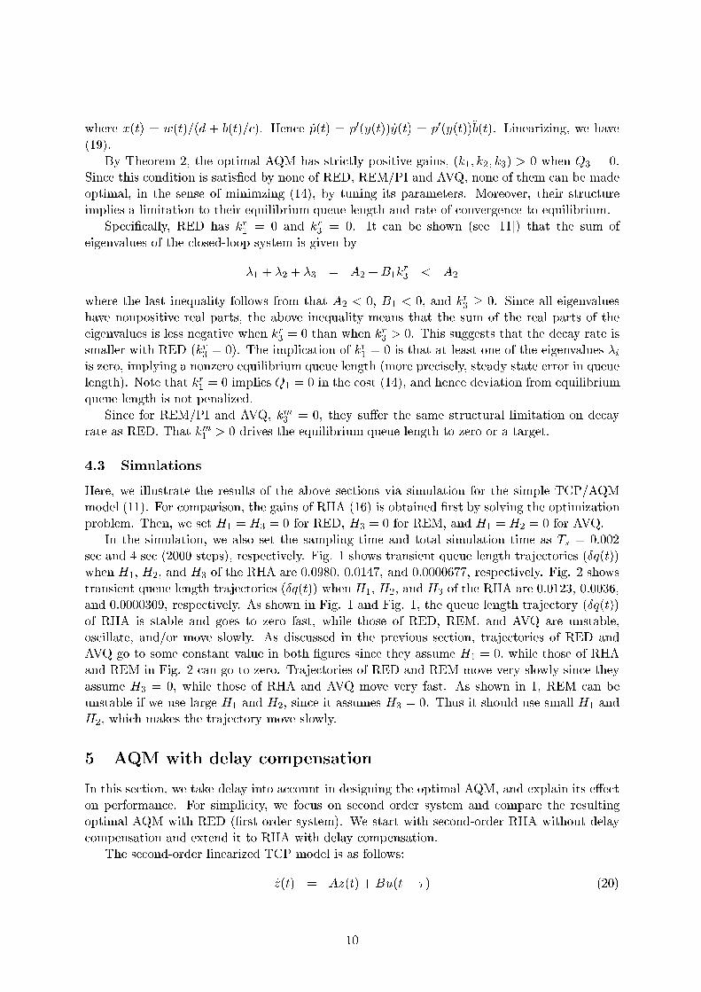
4.3 Simulations

Here, we illustrate the results of the above sections via simulation for the simple TCP/AQM

model (11). For comparison, the gains of RHA (16) is obtained �rst by solving the optimization

problem. Then, we set H1 = H3 = 0 for RED, H3 = 0 for REM, and H1 = H2 = 0 for AVQ.

In the simulation, we also set the sampling time and total simulation time as Ts = 0:002

sec and 4 sec (2000 steps), respectively. Fig. 1 shows transient queue length trajectories (Æq(t))

when H1, H2, and H3 of the RHA are 0:0980, 0:0147, and 0:0000677, respectively. Fig. 2 shows

transient queue length trajectories (Æq(t)) when H1, H2, and H3 of the RHA are 0:0123, 0:0036,

and 0:0000309, respectively. As shown in Fig. 1 and Fig. 1, the queue length trajectory (Æq(t))

of RHA is stable and goes to zero fast, while those of RED, REM, and AVQ are unstable,

oscillate, and/or move slowly. As discussed in the previous section, trajectories of RED and

AVQ go to some constant value in both �gures since they assume H1 = 0, while those of RHA

and REM in Fig. 2 can go to zero. Trajectories of RED and REM move very slowly since they

assume H3 = 0, while those of RHA and AVQ move very fast. As shown in 1, REM can be

unstable if we use large H1 and H2, since it assumes H3 = 0. Thus it should use small H1 and

H2, which makes the trajectory move slowly.

5 AQM with delay compensation

In this section, we take delay into account in designing the optimal AQM, and explain its e�ect

on performance. For simplicity, we focus on second order system and compare the resulting

optimal AQM with RED (�rst order system). We start with second-order RHA without delay

compensation and extend it to RHA with delay compensation.

The second-order linearized TCP model is as follows:

_z(t) = Az(t) +Bu(t� �) (20)

10

0 500 1000 1500 2000−0.1

0

0.1

0.2

0.3

0.4

0.5

0.6

Proposed RHA

step (2ms)

Qu

eu

e L

en

gth

Err

or

0 500 1000 1500 2000−0.2

−0.1

0

0.1

0.2

0.3

RED

step (2ms)

Qu

eu

e L

en

gth

Err

or

0 500 1000 1500 2000−150

−100

−50

0

50

100

REM

step (2ms)

Qu

eu

e L

en

gth

Err

or

0 500 1000 1500 20000

0.1

0.2

0.3

0.4

0.5

AVQ

step (2ms)

Qu

eu

e L

en

gth

Err

or

Figure 1: Queue length (Æq) trajectory

0 500 1000 1500 20000

0.2

0.4

0.6

0.8

1

Proposed RHA

step (2ms)

Qu

eu

e L

en

gth

Err

or

0 500 1000 1500 2000−0.2

0

0.2

0.4

0.6

0.8

RED

step (2ms)

Qu

eu

e L

en

gth

Err

or

0 500 1000 1500 2000−0.8

−0.6

−0.4

−0.2

0

0.2

0.4

0.6REM

step (2ms)

Qu

eu

e L

en

gth

Err

or

0 500 1000 1500 20000

0.2

0.4

0.6

0.8

1

AVQ

step (2ms)

Qu

eu

e L

en

gth

Err

or

Figure 2: Queue length (Æq) trajectory

11

where z(0) and fu(�); � 2 [��; 0]g are given,

z(t) =

�Æb(t)

Æ _b(t)

�; A =

�0 1

A1 A2

�B =

�0

B1

�

u(t) = Æp(t):

Throughout the rest of this section, for simplicity, we de�ne

a1 =A2 +

pA2

2 + 4A1

2; a2 =

A2 �pA2

2 + 4A1

2

a3 =1

a1 � a2loge

a2

a1(21)

e1 = e�a1� � e�a2� ; e2 = a1e�a1� � a2e

�a2�

e3 = a2e�a1� � a1e

�a2� (22)

B̂1 = �B1(a1 � a2)

e1: (23)

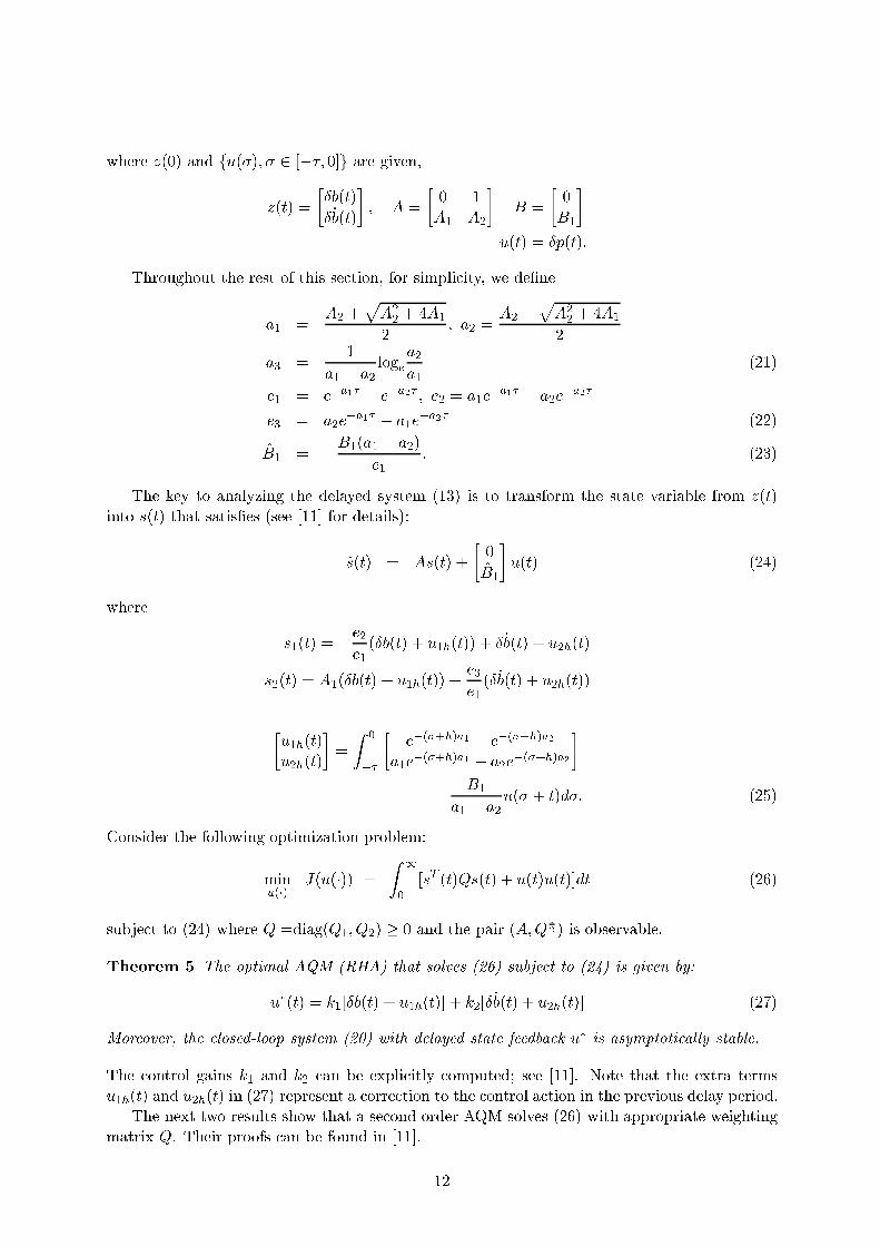
The key to analyzing the delayed system (13) is to transform the state variable from z(t)

into s(t) that satis�es (see [11] for details):

_s(t) = As(t) +

�0

B̂1

�u(t) (24)

where

s1(t) = �e2e1(Æb(t) + u1h(t)) + Æ _b(t) + u2h(t)

s2(t) = A1(Æb(t) + u1h(t)) +e3

e1(Æ _b(t) + u2h(t))

�u1h(t)

u2h(t)

�=

Z 0

��

�e�(�+h)a1 � e�(�+h)a2

a1e�(�+h)a1 � a2e

�(�+h)a2

�

B1

a1 � a2u(� + t)d�: (25)

Consider the following optimization problem:

minu(�)

J(u(�)) =

Z 1

0

[sT (t)Qs(t) + u(t)u(t)]dt (26)

subject to (24) where Q =diag(Q1; Q2) � 0 and the pair (A;Q1

2 ) is observable.

Theorem 5 The optimal AQM (RHA) that solves (26) subject to (24) is given by:

u�(t) = k1[Æb(t) + u1h(t)] + k2[Æ _b(t) + u2h(t)] (27)

Moreover, the closed-loop system (20) with delayed state feedback u� is asymptotically stable.

The control gains k1 and k2 can be explicitly computed; see [11]. Note that the extra terms

u1h(t) and u2h(t) in (27) represent a correction to the control action in the previous delay period.

The next two results show that a second order AQM solves (26) with appropriate weighting

matrix Q. Their proofs can be found in [11].

12

Theorem 6 Given AQM u(t) = [k1; k2]s(t) that satis�es A1+B̂1k1 and A2+B̂1k2 are negative,

it solves the receding horizon problem (26) with weights

Q1 =k21B̂

21 + 2k1A1B̂1

B̂21

Q2 =k22B̂

21 + 2k2A2B̂1 + 2k1B̂1

B̂21

:

Alternatively, an AQM can be speci�ed by the eigenvalues of the desired closed-loop system.

Theorem 7 Given the eigenvalues �1 and �2 of the closed-loop system of the transformed vari-

able s(t), they solves the receding horizon problem (26) with weights

Q1 =(�1�2)

2 �A21

B̂21

Q2 =�21 + �22 �A2

2 � 2A1

B̂21

:

We make several remarks on the RHA with delay compensation and interpret RED as an

approximation of RHA.

Theorem 5 shows that, at second order, under optimal AQM, the probability p(t) should

depend on both queue length and aggregate rate. Moreover, because of the delay, the control

should correct the error in input over the previous delay period, as represented by uih(t).

As before we model RED by (note the input is Æp(t) not Æ _p(t) as in the third order system):

Æp(t) = kr1Æb(t)

Hence RED sets both k2 = 0 and the history of past inputs uih(t) to zero. This reduces the

decay rate of RED; see [11].

6 Simulation Examples

Here, we illustrate the delay e�ect of AQM algorithms via NS simulation for the nonlinear model.

In NS simulation, we set N and c as 100 and 4000, respectively. For implementation of RHA,

we set a target queue length as b� = 175 packets/sec.

We set Q1 =�

B̂2

1

, Q2 =2p

A2

1+B̂2

1�Q1�A

2

2�2A1

B̂2

1

, and Ts = 0:04 sec, respectively where Ts is a

sampling time.

We compare RHA (27) with RHA (27) (with uih = 0) and RED (u(t) = �Æq(t), � � 0:001).

Fig. 3 shows queue length trajectories (q(t)) when � = 0:25 sec. Fig. 4 shows queue length

trajectories (q(t)) when � = 0:15 sec. Figures show that queue length q(t) of RHA (27) goes

to the target queue length 175 pkts, almost two or three times faster than RED, while that of

RHA (27) (with uih(t) = 0) oscillate. This result illustrates that we should consider the delay

term when we design AQM algorithms.

7 Conclusion

In this paper, we propose a uni�ed mathematical framework based on receding horizon control

for analyzing and designing AQM (Active Queue Management) algorithms in stabilizing TCP

13

0 5 10 15 20 25 300

200

400

600

800

1000

time (sec.)

Queue L

ength

(pkts

.)

RHA with DCRED

0 5 10 15 20 25 300

200

400

600

800

1000

time (sec.)

Queue L

ength

(pkts

.)

RHA with DCRHA with no DC

Figure 3: Queue length (q) trajectory

0 5 10 15 20 25 300

200

400

600

800

time (sec.)

Queue L

ength

(pkts

.)

RHA with DCRED

0 5 10 15 20 25 300

100

200

300

400

500

600

time (sec.)

Queue L

ength

(pkts

.)

RHA with DCRHA with no DC

Figure 4: Queue length (q) trajectory

14

(Transfer Control Protocol). The proposed framework is based on a dynamical system of the

given TCP and a linear quadratic cost on transients in queue length and ow rates. We derive

the optimal receding horizon AQMs (RHAs) that stabilizes the linearized dynamical system with

the minimum cost. Conversely, we show that any AQM with an appropriate structure solves the

same optimal control problem with appropriate weighting matrix. We interpret existing AQM's

such as RED, REM, PI and AVQ as di�erent approximations of the optimal AQM, and discuss

the impact of these approximations on performance.

Acknowledgement: The �rst author acknowledges the support of the Post-doctoral Fellowship

Program of Korean Science & Engineering Foundation (KOSEF). We would like to thank to

Sanjeewa Athuraliya for his help of NS-simulation.

References

[1] S. Athuraliya, V. H. Li, S. H. Low, and Q. Yin. REM: active queue management. IEEE Network,

May/June 2001. Extended version in Proceedings of ITC17, Salvador, Brazil, September 2001.

http://netlab.caltech.edu.

[2] H. Chen and F. Allgower. A quasi-in�nite horizon nonlinear model predictive control scheme with

guaranteed stability. Automatica, 34:1205{1217, 1998.

[3] S. Floyd and V. Jacobson. Random early detection gateways for congestion avoidance. IEEE/ACM

Trans. on Networking, 1(4):397{413, August 1993. ftp://ftp.ee.lbl.gov/papers/early.ps.gz.

[4] G. De Nicolao and L. Magni and R. Scattolini. Stabilizing receding horizon control of nonlinear

time-varying systems. IEEE Trans. Automat. Contr., 43(7):1030 { 1036, 1998.

[5] C. Hollot, V. Misra, D. Towsley, and W.-B. Gong. A control theoretic analysis of RED. In Proceedings

of IEEE Infocom, April 2001. http://www-net.cs.umass.edu/papers/papers.html.

[6] C. Hollot, V. Misra, D. Towsley, and W.-B. Gong. On designing improved controllers for AQM

routers supporting TCP ows. In Proceedings of IEEE Infocom, April 2001. http://www-net.cs.

umass.edu/papers/papers.html.

[7] F. P. Kelly. Charging and rate control for elastic traÆc. European Transactions on Telecommunica-

tions, 8:33{37, 1997. http://www.statslab.cam.ac.uk/~frank/elastic.html.

[8] F. P. Kelly. Mathematical modelling of the Internet. In Proc. 4th International Congress on Industrial

and Applied Mathematics, July 1999. http://www.statslab.cam.ac.uk/~frank/mmi.html.

[9] F. P. Kelly, A. Maulloo, and D. Tan. Rate control for communication networks: Shadow prices,

proportional fairness and stability. Journal of Operations Research Society, 49(3):237{252, March

1998.

[10] K. B. Kim. Disturbance attenuation of for input-constrained discrete time-invariant systems via

receding horizon control. To appear in IEEE Transactions on Automatic Control, 2001.

[11] K. B. Kim and S. H. Low. Analysis and design of AQM based on receding horizon control in

stabilizing TCP. To be submitted for publication, March, 2002.

[12] M. V. Kothare, V. Balakrishnan, and M. Morari. Robust constrained model predictive control using

linear matrix inequalities. Automatica, 32:1361 { 1379, 1996.

[13] S. Kunniyur and R. Srikant. A time{scale decomposition approach to adaptive ECN marking. In

Proceedings of IEEE Infocom, April 2001. http://comm.csl.uiuc.edu:80/~srikant/pub.html.

[14] S. Kunniyyr and R. Srikant. End{to{end congestion control schemes: utility functions, random losses

and ECN marks. In Proceedings of IEEE/INFOCOM, 2000. http://www.ieee-infocom.org/2000/

papers/401.ps.

15

[15] S. Kunniyyr and R. Srikant. Analysis and design of an adaptive virtual queue (AVQ) algorithm

for active queue management. In Proceedings of ACM/SIGCOMM, 2001. http://comm.csl.uiuc.

edu/~srikant/pub.html.

[16] W. H. Kwon and K. B. Kim. On stabilizing receding horizon controls for linear continuous time-

invariant systems. IEEE Transactions on Automatic Control, 45(8):1329{1334, 2000.

[17] S. H. Low. A duality model of TCP ow controls. In Proceedings of ITC Specialist Seminar on IP

TraÆc Measurement, Modeling and Management, September 18-20 2000. http://netlab.caltech.

edu.

[18] S. H. Low and D. E. Lapsley. Optimization ow control, I: basic algorithm and convergence.

IEEE/ACM Transactions on Networking, 7(6):861{874, December 1999. http://netlab.caltech.

edu.

[19] S. H. Low, F. Paganini, J. Wang, S. A. Adlakha, and J. C. Doyle. Dynamics of TCP/AQM and a

scalable control. In Proceedings of IEEE Infocom, June 2002.

[20] S. H. Low, L. Peterson, and L. Wang. Understanding Vegas: a duality model. J. of ACM, to appear,

2002. http://netlab.caltech.edu/pub.html.

[21] F. Paganini, J. C. Doyle, and S. H. Low. Scalable laws for stable network congestion control. In

Proceedings of Conference on Decision and Control, December 2001. http://www.ee.ucla.edu/

~paganini.

[22] J. B. Rawlings and K. R. Muske. The stability of constrained receding horizon control. IEEE Trans.

Automat. Contr., 38(10):1512 { 1516, 1993.

16