calypso - geodynamics · preface calypso is a program package of magnetohydrodynamics (mhd)...

COMPUTATIONAL INFRASTRUCTURE FOR GEODYNAMICS (CIG)

CalypsoUser Manual

Version 1.2

Hiroaki Matsuiwww.geodynamics.org

PrefaceCalypso is a program package of magnetohydrodynamics (MHD) simulations in a rotatingspherical shell for geodynamo problems. This package consists of the simulation program,preprocessing program, post processing program to generate field data for visualizationprograms, and several small utilities. The simulation program runs on parallel computingsystems using MPI and OpenMP parallelization.

1

Contents1 Introduction 6

2 History 62.1 Updates for Ver 1.1 . . . . . . . . . . . . . . . . . . . . . . . . . . . . . 72.2 Updates for Ver 1.2 . . . . . . . . . . . . . . . . . . . . . . . . . . . . . 8

3 Acknowledgements 9

4 Citation 9

5 Model of Simulation 105.1 Governing equations . . . . . . . . . . . . . . . . . . . . . . . . . . . . 105.2 Spherical harmonics expansion . . . . . . . . . . . . . . . . . . . . . . . 125.3 Evaluation of Coriolis term . . . . . . . . . . . . . . . . . . . . . . . . . 125.4 Boundary conditions . . . . . . . . . . . . . . . . . . . . . . . . . . . . 13

5.4.1 Non-slip boundary . . . . . . . . . . . . . . . . . . . . . . . . . 135.4.2 Free-slip boundary . . . . . . . . . . . . . . . . . . . . . . . . . 135.4.3 Fixed rotation rate . . . . . . . . . . . . . . . . . . . . . . . . . 135.4.4 Fixed homogenous temperature . . . . . . . . . . . . . . . . . . 145.4.5 Fixed homogenous heat flux . . . . . . . . . . . . . . . . . . . . 145.4.6 Fixed composition . . . . . . . . . . . . . . . . . . . . . . . . . 145.4.7 Fixed composition flux . . . . . . . . . . . . . . . . . . . . . . . 145.4.8 Connection to the magnetic potential field . . . . . . . . . . . . . 155.4.9 Magnetic boundary condition for center . . . . . . . . . . . . . . 165.4.10 Pseudo-vacuum magnetic boundary condition . . . . . . . . . . . 16

6 Installation 176.1 Library Requirements . . . . . . . . . . . . . . . . . . . . . . . . . . . . 176.2 Known problems . . . . . . . . . . . . . . . . . . . . . . . . . . . . . . 186.3 Directories . . . . . . . . . . . . . . . . . . . . . . . . . . . . . . . . . . 186.4 Doxygen . . . . . . . . . . . . . . . . . . . . . . . . . . . . . . . . . . . 196.5 Install using configure command . . . . . . . . . . . . . . . . . . . 19

6.5.1 Configuration using configure command . . . . . . . . . . . 196.5.2 Compile . . . . . . . . . . . . . . . . . . . . . . . . . . . . . . . 216.5.3 Clean . . . . . . . . . . . . . . . . . . . . . . . . . . . . . . . . 226.5.4 Install . . . . . . . . . . . . . . . . . . . . . . . . . . . . . . . . 22

6.6 Install without using configure . . . . . . . . . . . . . . . . . . . . . . . 22

2

6.7 Install using cmake . . . . . . . . . . . . . . . . . . . . . . . . . . . . . 23

7 Simulation procedure 25

8 Examples 298.1 Examples for preprocessing program . . . . . . . . . . . . . . . . . . . . 298.2 Examples of dynamo benchmark . . . . . . . . . . . . . . . . . . . . . . 29

8.2.1 Data files and directories for Case 0 . . . . . . . . . . . . . . . . 318.2.2 Data files and directories for Case 1 . . . . . . . . . . . . . . . . 318.2.3 Data files and directories for Case 2 . . . . . . . . . . . . . . . . 328.2.4 Data files and directories for Compositional Case 1 . . . . . . . . 32

8.3 Example of data assembling program . . . . . . . . . . . . . . . . . . . . 338.4 Example of treatment of heat and composition source term . . . . . . . . 338.5 Example of thermal and compositional boundary conditions by external file 34

9 Preprocessing program (gen sph grid) 359.1 Position of radial grid . . . . . . . . . . . . . . . . . . . . . . . . . . . . 369.2 Control file (control sph shell) . . . . . . . . . . . . . . . . . . . 369.3 Spectrum index data . . . . . . . . . . . . . . . . . . . . . . . . . . . . 389.4 Finite element mesh data . . . . . . . . . . . . . . . . . . . . . . . . . . 389.5 Radial grid data . . . . . . . . . . . . . . . . . . . . . . . . . . . . . . . 389.6 How to define spatial resolution and parallelization? . . . . . . . . . . . . 39

10 Simulation program (sph mhd) 4110.1 Control file . . . . . . . . . . . . . . . . . . . . . . . . . . . . . . . . . 4310.2 Spectrum data for restarting . . . . . . . . . . . . . . . . . . . . . . . . . 4610.3 Thermal and compositional boundary condition data file . . . . . . . . . 4710.4 Field data for visualization . . . . . . . . . . . . . . . . . . . . . . . . . 47

10.4.1 Distributed VTK data . . . . . . . . . . . . . . . . . . . . . . . . 4910.4.2 Merged VTK data . . . . . . . . . . . . . . . . . . . . . . . . . 4910.4.3 Merged XDMF data . . . . . . . . . . . . . . . . . . . . . . . . 50

10.5 Cross section data (Parallel Surfacing module . . . . . . . . . . . . . . . 5110.5.1 Control file . . . . . . . . . . . . . . . . . . . . . . . . . . . . . 52

10.6 Isosurface data . . . . . . . . . . . . . . . . . . . . . . . . . . . . . . . 5310.6.1 Control file . . . . . . . . . . . . . . . . . . . . . . . . . . . . . 53

10.7 Mean square amplitude data . . . . . . . . . . . . . . . . . . . . . . . . 5410.7.1 Volume average data . . . . . . . . . . . . . . . . . . . . . . . . 5510.7.2 Volume spectrum data . . . . . . . . . . . . . . . . . . . . . . . 5510.7.3 layered spectrum data . . . . . . . . . . . . . . . . . . . . . . . 57

3

10.8 Gauss coefficient data [gauss coef prefix].dat . . . . . . . . . . 5810.9 Spectrum monitor data [picked sph prefix].dat . . . . . . . . . 5910.10Nusselt number data [nusselt number prefix].dat . . . . . . . 59

11 Data transform program(sph snapshot and sph zm snapshot) 61

12 Initial field generation program(sph initial field) 6312.1 Definition of the initial field . . . . . . . . . . . . . . . . . . . . . . . . 64

13 Initial field modification program(sph add initial field) 67

14 Check program for dynamo benchmark(sph dynamobench) 6814.1 Dynamo benchmark data dynamobench.dat . . . . . . . . . . . . . . 69

15 Data assemble program (assemble sph) 7115.1 Format of control file . . . . . . . . . . . . . . . . . . . . . . . . . . . . 71

16 Module dependency program (module dependency) 73

17 Time averaging programs 7317.1 Averaging for mean square and power spectrum

(t ave sph mean square) . . . . . . . . . . . . . . . . . . . . . . . 7317.2 Averaging for picked harmonics mode data

(t ave picked sph coefs) . . . . . . . . . . . . . . . . . . . . . . 73

18 Visualization using field data 74

Appendices 78

Appendix A Definition of parameters for control files 78A.1 data files def . . . . . . . . . . . . . . . . . . . . . . . . . . . . . 78A.2 phys values ctl . . . . . . . . . . . . . . . . . . . . . . . . . . . . 79A.3 time evolution ctl . . . . . . . . . . . . . . . . . . . . . . . . . . 79A.4 boundary condition . . . . . . . . . . . . . . . . . . . . . . . . . 79A.5 forces define . . . . . . . . . . . . . . . . . . . . . . . . . . . . . 83A.6 dimensionless ctl . . . . . . . . . . . . . . . . . . . . . . . . . . 83

4

A.7 coefficients ctl . . . . . . . . . . . . . . . . . . . . . . . . . . . 84A.7.1 thermal . . . . . . . . . . . . . . . . . . . . . . . . . . . . . . 84A.7.2 momentum . . . . . . . . . . . . . . . . . . . . . . . . . . . . . 84A.7.3 induction . . . . . . . . . . . . . . . . . . . . . . . . . . . . 85A.7.4 composition . . . . . . . . . . . . . . . . . . . . . . . . . . 86

A.8 temperature define . . . . . . . . . . . . . . . . . . . . . . . . . 86A.9 time step ctl . . . . . . . . . . . . . . . . . . . . . . . . . . . . . . 87A.10 new time step ctl . . . . . . . . . . . . . . . . . . . . . . . . . . . 88A.11 restart file ctl . . . . . . . . . . . . . . . . . . . . . . . . . . . 88A.12 time loop ctl . . . . . . . . . . . . . . . . . . . . . . . . . . . . . . 89A.13 sph monitor ctl . . . . . . . . . . . . . . . . . . . . . . . . . . . . 90A.14 visual control . . . . . . . . . . . . . . . . . . . . . . . . . . . . . 93A.15 cross section ctl . . . . . . . . . . . . . . . . . . . . . . . . . . 93

A.15.1 surface define . . . . . . . . . . . . . . . . . . . . . . . . 93A.15.2 output field define . . . . . . . . . . . . . . . . . . . . . 95A.15.3 isosurf define . . . . . . . . . . . . . . . . . . . . . . . . 96A.15.4 field on isosurf . . . . . . . . . . . . . . . . . . . . . . . 97

A.16 num domain ctl . . . . . . . . . . . . . . . . . . . . . . . . . . . . . 97A.17 num grid sph . . . . . . . . . . . . . . . . . . . . . . . . . . . . . . 98A.18 new data files def . . . . . . . . . . . . . . . . . . . . . . . . . . 100A.19 newrst magne ctl . . . . . . . . . . . . . . . . . . . . . . . . . . . 100

Appendix B GNU GENERAL PUBLIC LICENSE 101

5

1 IntroductionCalypso is a program package for magnetohydrodynamics (MHD) simulations in a ro-tating spherical shell for geodynamo problems. This package consists of the simulationprogram, preprocessing program, post processing program to generate field data for visu-alization programs, and several small utilities. The simulation program runs on parallelcomputing systems using MPI and OpenMP parallelization.

Calypso solves the equations that govern convection and magnetic-field generation in arotating spherical shell. Flow is driven by thermal or compositional buoyancy in a Boussi-nesq fluid. Calypso also support various boundary conditions (e.g. fixed temperature, heatflux, composition, and compositional flux), and permits a conductive and rotatable innercore. Results are written as spherical harmonics coefficients, Gauss coefficients for the re-gion outside of the fluid shell, and field data in Cartesian coordinate for easily visualizationwith a number of visualization programs.

This user guide describes the essentials of the magnetohydrodynamics theory andequations behind Calypso, and provides instructions for the configuration and executionof Calypso.

2 HistoryCalypso has its origins in two earlier projects. One is a dynamo simulation code writtenby Hiroaki Matsui in 1990’s using a spectral method. This code solves for the poloidaland toroidal spectral coefficients, like Calypso, but it calculates the nonlinear terms in thespectral domain using a parallelization for SMP architectures. The other project is thethermal convection version of GeoFEM, which is Finite Element Method (FEM) platformfor massively parallel computational environment, originally written by Hiroshi Okuda in2000. Under GeoFEM Project, Lee Chen developed cross sectioning, iso-surfacing, andvolume rendering modules for data visualization for parallel computations..

Hiroaki Matsui was responsible for adding routines to GeoFEM to perform magneto-hydrodynamics simulation in a rotating frame. In 2002 this code successfully performeddynamo simulations in a rotating spherical shell using insulating magnetic boundary con-ditions. The following year Matsui implemented a subgrid scale (SGS) model in the FEMdynamo model in collaboration with Bruce Buffett. A module to solve for double diffusiveconvection was added to the FEM dynamo model by Hiroaki Matsui in 2009.

Progress in understanding the role of subgrid scale models in magnetohydrodynamicsimulations relies on quantitative estimates for the transfer of energy between spatialscales. This information is most easily obtained from a spherical harmonic expansionof the simulation results, even when the simulation is performed by FEM. Hiroaki Matsui

6

implemented the spherical harmonic transform in 2007 using a combination of MPI andOpenMP, and later included the spherical harmonic transform routines into his old dynamocode to create Calypso. Additional software in the program package for visualization isbased on data formats from the FEM model. In addition, the control parameter file formatis adapted from the input formats used in GeoFEM.

Calypso Ver. 1.0 supports the following features and capabilities

• Magnetohydrodynamics simulation for a Boussinesq fluid in a rotating sphericalshell.

• Convection driven by thermal and compositional buoyancy.

• Temperature or heat flux is fixed at boundaries

• Composition or compositional flux is fixed at boundaries

• Non-slip or free-slip boundary conditions

• Outside of the fluid shell is electrically insulated or pseudo vacuum boundary.

• A conductive inner core with the same conductivity as the surrounding fluid

• A rotating inner core driven by the magnetic and viscous torques.

2.1 Updates for Ver 1.1In Version 1.1, a number of bug fixes and additional comments for Doxygen are completed.The following large bugs are fixed:

• configure command is updated to find appropriate GNU make command. (seeSection 6.1)

• Label for radial grid type in the file ctl_sph_shell raidal_grid_type_ctlis changed to radial_grid_type_ctl. If the old name is used in the controlfile, program gen_sph_grid will crash.

And, the following features are implemented

• New ordering is used for spherical harmonics data to reduce communication time.The old version of spectrum indexing data, which is generated by gen_sph_gridsin Ver. 1.0 is also supported in Ver. 1.1.

7

• Evaluation of Coriolis term is updated. Now, Adams-Gaunt integrals are evaluatedin the initialization process in the simulation program sph_mhd, so the data file forAdams-Gaunt integrals which is made by gen_sph_grids is not required.

• Add a program sph_add_initial_field. to modify existed initial field data.This program is used to modify or add new fields in spectrum data. (See Section13.)

• Heat and composition source terms are implemented. These source terms are fixedwith time, and defined as spectrum data. The source terms are defined by usinginitial field generation programsph_initial_field or sph_add_initial_field. (See section 12 and13.)

• The boundary conditions for temperature and composition can be defined by usingspherical harmonics coefficients. (i.e. inhomogeneous boundary conditions can beapplied.) These boundary conditions are defined by using single external data file.(See Section 10.3)

2.2 Updates for Ver 1.2In Version 1.2, the following features are implemented:

• To reduce the number of calculation, Legendre transform is calculated with takingaccount to the symmetry with respect to the equator. Time for Legendre transformis approximately half of that in Ver 1.1.

• BLAS library can be used for the Legendre transform optionally.

• Cross sectioning and isosurfacing module are newly implemented. These modulesare re-written by Fortran90 from the parallel sectioning modules in GeoFEM byLee Chen in C, and some features are added for visualizations of geodynamo simu-lations. See section ?? and 10.6.

• Initial data assemble program assemble_mhd is parallelized. This program canperform with any number of MPI processes, but we recommend to run the programwith one process or the same number of processes as the number of subdomains forthe target configuration which is defined by num_new_domain_ctl. See section13.

• The time and time step information in the restart data can be modifield by assemble_mhd.See section 13

8

3 AcknowledgementsCalypso was primarily developed by Dr. Hiroaki Matsui in collaboration with Prof. BruceBuffett at the University of California, Berkeley. The following NSF grants supported thedevelopment of Calypso,

• B.A. Buffett, NSF EAR-0509893; Models of sub-grid scale turbulence in the Earthscore and the geodynamo; 2005 - 2007.

• B.A. Buffett and D. Lathrop, NSF EAR-0652882; CSEDI Collaborative Research:Integrating numerical and experimental geodynamo models, 2007 - 2009

• B.A. Buffett, NSF EAR-1045277; Development and application of turbulence mod-els in numerical geodynamo simulations ; 2010 - 2012

4 CitationComputational Infrastructure for Geodynamics (CIG) and the Calypso developers aremaking the source code to Calypso available to researchers in the hope that it will aid theirresearch and teaching. A number of individuals have contributed a significant amount oftime and energy into the development of Calypso. We request that you cite the appropriatepapers and make acknowledgements as necessary. The Calypso development team asksthat you cite the following papers:

Matsui, H., E. King, and B.A. Buffett, Multi-scale convection in a geodynamo simula-tion with uniform heat flux along the outer boundary, Geochemistry, Geophysics, Geosys-tems, 15, 3212 – 3225, 2014.

9

5 Model of Simulation

5.1 Governing equations

Crust

Mantle

Outer CoreInner Core

CMBICB

Conductive fluid

InsulatorConductive solid or insulator

rori

L

Figure 1: Rotating spherical shell modeled on the Earth’s outer core.

This model performs a magnetohydrodynamics (MHD) simulation in a rotating spher-ical shell modeled on the Earth’s outer core (see Figure 1). We consider a spherical shellfrom the inner core boundary (ICB) to the core mantle Boundary (CMB) in a rotatingframe which constantly rotates with angular velocity Ω = Ωz. The fluid shell is filled witha conductive fluid with constant diffusivities (kinematic viscosity ν, magnetic diffusivityη, thermal diffusivity κT , and compositional diffusivity κC). The inner core (0 < r < ri) issolid, and may be considered an electrical insulator or may have the same conductivity asthe outer core. We assume that the region outside of the core is an electrical insulator. Therotating spherical shell is filled with Boussinesq modeled fluid. The governing equationsof the MHD dynamo problem are the following,

∂u

∂t+ (ω × u) = −∇

(P +

1

2u2)− ν∇×∇× u

−2Ω (z × u) +

(ρ

ρ0g

)+

1

ρ0(J ×B) ,

10

∂B

∂t= −η∇×∇×B +∇× (u×B) ,

∂T

∂t+ (u · ∇)T = κT∇2T + qT ,

∂C

∂t+ (u · ∇)C = κC∇2C + qC ,

∇ · u = ∇ ·B = 0,

ω = ∇× u,

and

J =1

µ0

∇×B,

where, u, ω, P , B , J , T , C, qT , and qC are the velocity, vorticity, pressure, magneticfield, current density, temperature, compositional variation, heat source, and source of lightelement, respectively. Coefficients in the governing equations are the kinetic viscosityν, thermal diffusivity κT , compositional diffusivity κC , and magnetic diffusivity η. Thedensity ρ is written as a function of T , C, average density ρ0, thermal expansion αT , anddensity ratio of light element to main composition αC ,

ρ = ρ0 [1− αT (T − T0)− αC (C − C0)]

In Calypso, the vorticity equation and divergence of the momentum equation are used forsolving u, ω, and P as,

∂ω

∂t+∇× (ω × u) = −ν∇×∇× ω − 2Ω∇× (z × u)

+∇×(ρ

ρ0g

)+

1

ρ0∇× (J ×B) ,

and

∇ · (ω × u) = −∇2

(P +

1

2u2)− 2Ω∇ · (z × u)

+∇ ·(ρ

ρ0g

)+

1

ρ0∇ · (J ×B) .

11

5.2 Spherical harmonics expansionIn Calypso, fields are expanded into spherical harmonics. A scalar field (for example,temperature T (r, θ, φ)) is expanded as

T (r, θ, φ) =L∑l=0

l∑m=−l

Tml (r)Y ml (θ, φ),

where Y ml are the spherical harmonics. Solenoidal fields (e.g. velocity u, vorticity ω,

magnetic field B, and current density J ) are decomposed into poloidal and toroidal com-ponents. For example, the magnetic field is described as

B(r, θ, φ) =L∑l=1

l∑m=−l

(B mSl + B m

Tl ) ,

where

B mSl (r, θ, φ) = ∇×∇× (B m

Sl (r)Y ml (θ, φ)r) ,

B mTl (r, θ, φ) = ∇× (B m

Tl (r)Y ml (θ, φ)r) .

The spherical harmonics are defined as real functions. Pml cos (mφ) is assigned for

positive m, Pml sin (mφ) is assigned for negative m, where Pm

l are Legendre polynomi-als. Because Schmidt quasi normalization is used for the Legendre polynomials Pm

l , theorthogonality relation for the spherical harmonics is∫

Y ml Y

m′

l′ sin θdθdφ = 4π1

2l + 1δll′δmm′ ,

where, δll′ is Kronecker delta.

5.3 Evaluation of Coriolis termThe curl of the Coriolis force−2Ω∇×(z × u) is evaluated in the spectrum space using thetriple products of the spherical harmonics. These 3j-symbols (or Gaunt integral GMmm′

Lll′

and Elsasser integral EMmm′

Lll′ ) are written as

GMmm′

Lll′ =

∫Y ML Y m

l Ym′

l′ sin θdθdφ,

EMmm′

Lll′ =

∫Y ML

(∂Y m

l

∂θ

∂Y m′

l′

∂φ− ∂Y m

l

∂φ

∂Y m′

l′

∂θ

)dθdφ.

The Gaunt integral 1/(4π)GMmm′

Lll′ and Elsasser integral 1/(4π)EMmm′

Lll′ for the Coriolisterms are evaluated in the simulation program.

12

5.4 Boundary conditionsCalypso currently supports the following boundary conditions for velocity u, magneticfield B, temperature T , and composition variation C. These boundary conditions aredefined in the control file control_MHD.

5.4.1 Non-slip boundary

The velocity u is set to be 0 at the boundary. For poloidal and toroidal coefficients ofvelocity, U m

Sl (r) and U mTl (r), the boundary condition can be described as

U mSl (r) =

∂U mSl

∂r= 0,

and

U mTl (r) = 0.

5.4.2 Free-slip boundary

For a free slip boundary, shear stress and radial flow vanish at the boundary. The boundarycondition for poloidal and toroidal coefficients are described as

U mSl (r) =

∂2

∂r2

(1

rU mSl (r)

)= 0,

and∂

∂r

(1

r2U mTl (r)

)= 0.

5.4.3 Fixed rotation rate

If the boundary rotates with a rotation vector Ωb = (Ωbx,Ωby,Ωbz), the boundary condi-tions for poloidal and toroidal coefficients are described as

U mSl (r) =

∂U mSl

∂r= 0,

U 1sT1 (r) = r2Ωby,

U 0T1(r) = r2Ωbz,

U 1cT1 (r) = r2Ωbx,

and

U mTl (r) = 0 for l > 2.

13

5.4.4 Fixed homogenous temperature

When a constant temperature Tb is is applied, the spherical harmonic coefficients are

T 00 (r) = Tb,

and

Tml (r) = 0 for l > 1.

5.4.5 Fixed homogenous heat flux

A constant heat flux is imposed by setting the radial temperature gradient to FTb. Thespherical harmonic coefficients are

∂T 00

∂r= FTb,

and

∂Tml∂r

= 0 for l > 1.

5.4.6 Fixed composition

When a constant composition Cb is applied, the spherical harmonic coefficients are

C00(r) = Cb,

and

Cml (r) = 0 for l > 1.

5.4.7 Fixed composition flux

A constant composition flux is imposed by setting the radial composition gradient to FCb.The spherical harmonic coefficients are

∂C00

∂r= FCb,

and

∂Cml

∂r= 0 for l > 1.

14

5.4.8 Connection to the magnetic potential field

If the regions outside the fluid shell are assumed to be electrical insulators, current densityvanishes in the electric insulator

J ext = 0,

where the suffix ext indicates fields outside of the fluid shell. At the boundaries of the fluidshell, the magnetic field Bfluid, current density Jfluid , and electric field Efluid in theconductive fluid satisfy:

(Bfluid −Bext) = 0,

(Jfluid − J ext) · r = 0,

and

(Efluid −Eext)× r = 0,

where, r is the radial unit vector (i.e. normal vector for the spherical shell boundaries).Consequently, radial current density J vanishes at the boundary as

J · r = 0 at r = ri, ro

In an electrical insulator the magnetic field can be described as a potential field

Bext = −∇Wext,

where Wext is the magnetic potential. The boundary conditions can be satisfied by con-necting the magnetic field in the fluid shell at boundaries to the potential fields. The mag-netic field is connected to the potential field in an electrical insulator. At CMB (r = ro),the boundary condition can be described by the poloidal and toroidal coefficients of themagnetic field as

l

rB mSl (r) = −∂B

mSl

∂r,

and

B mTl (r) = 0.

If the inner core is also assumed to be an insulator, the magnetic boundary conditionsfor ICB (r = ri) can be described as

l + 1

rB mSl (r) =

∂B mSl

∂r,

and

B mTl (r) = 0.

15

5.4.9 Magnetic boundary condition for center

If the inner core has the same conductivity as the outer core, we solve the induction equa-tion for the inner core as for the outer core with the boundary conditions for the center.The poloidal and toroidal coefficients at center are set to

B mSl (0) = B m

Tl (0) = 0.

5.4.10 Pseudo-vacuum magnetic boundary condition

Under the pseudo-vacuum boundary condition, the magnetic field has only a radial com-ponent at the boundaries. Considering the conservation of the magnetic field, the magneticboundary condition will be

∂

∂r

(r2Br

)= Bθ = Bφ = 0 at r = ri, ro.

The present boundary condition is also described by using the poloidal and toroidal coef-ficients as

∂B mSl

∂r= B m

Tl (r) = 0 at r = ri, ro.

16

6 Installation

6.1 Library RequirementsCalypso requires the following libraries.

• GNU make

• MPI libraries (OpenMPI, MPICH, etc)

• FFTPACK Ver 5.1D (http://people.sc.fsu.edu/˜jburkardt/f_src/fftpack5.1d/fftpack5.1d.html). The source files for FFTPACK are in-cluded in src/EXTERNAL libs directory.

Linux and Max OS X use GNU make as a default ’make’ command, but some system (e.g.BSD or SOLARIS) does not use GNU make as default. configure command searchesand set correct GNU make command.

In addition, the following environment and libraries can be used (optional).

• OpenMP

• BLAS

• FFTW version 3 (http://www.fftw.org) including Fortran wrapper

• PARALLEL HDF5 (http://www.hdfgroup.org/HDF5/PHDF5) includingFortran wrapper.

Note: Calypso does NOT use MPI and OpenMP features in FFTW3.In the most of platforms, the Fourier transform by FFTW is faster than that by FFT-

PACK.HDF5 is used for field data output with XDMF format instead of VTK format. The

comparison of field data format is described in section refsec:VTK.OpenMP is used for the parallelization under the shared memory. Better choice to use

both MPI and OpenMP parallelization (so-called Hybrid parallelization) or only using MPI(so-called flat MPI) is depends on the computational platform and compiler. For example,flat MPI has much better performance on Linux cluster with Intel Xeon processors andwith Intel fortran compiler, but Hybrid model has better performance on Hitachi SR16000with Power 6 processors.

17

http://people.sc.fsu.edu/~jburkardt/f_src/fftpack5.1d/fftpack5.1d.html

http://people.sc.fsu.edu/~jburkardt/f_src/fftpack5.1d/fftpack5.1d.html

http://www.fftw.org

http://www.hdfgroup.org/HDF5/PHDF5

6.2 Known problemsFFTPACK and Intel compiler

FFTPACK fails to compile with Intel fortran using the ‘-warn all’ option. Currentlythe ‘-warn all’ option is excluded by Makefile when FFTPACK is compiled.

Homebrew’s FFTW3 on Mac OS X

Calypso uses Fortran wrappers in FFTW3. If FFTW3 is installed using Homebrew for MacOS X (http://mxcl.github.com/homebrew/), the required fortran wrappers arenot installed. In this case, please install FFTW3 with Fortran wrappers with another pack-age manager (Macports (http://www.macports.org, for example), build FFTW3by yourself including the Fortran wrapper, or turn off FFTW3 features in Calypso.

XL fortran

In XL fortran, preprocessor options is not specified by -D..., but -Wf, ’-D...’.Pleease edit preprocessor macro opthion F90CPPFLAGS in work/Makefile by aneditor.

Cross compiler support

configure command in Calypso does not support cross compilation. If you want tocompile with a cross compiler, please set the variables in Makefile manually (see section6.6)

6.3 DirectoriesThe top directory of Calypso (ex. [CALYPSO_HOME]) contains the following directories.

% cd [CALYPSO_HOME]% lsCMakeLists.txt Makefile.in configure.in examplesINSTALL bin doc srcLICENSE configure doxygen work

bin: directory for executable files

cmake: directory for cmake configurations

18

http://mxcl.github.com/homebrew/

http://www.macports.org

cmake: directory for document generated by doxygen

doc: documentations

examples: examples

src: source files

work: work directory. Compile is done in this directory.

6.4 DoxygenDoxygen (http://www.doxygen.org) is an powerful document generation tool fromsource files. We only save a configuration file in this directory because thousands of htmlfiles generated by doxygen. The documents for source codes are generated by the follow-ing command:

% cd [CALYPSO_HOME]/doxygen% doxygen ./Doxyfile_CALYPSO

The html documents can see by opening [CALYPSO_HOME]/doxygen/html/index.html.Automatically generated documentation is also available on the CIG website at http://www.geodynamics.org/cig/software/calypso/.

6.5 Install using configure command6.5.1 Configuration using configure command

Calypso uses the configure script for configuration to install. The simplest way to installprograms is the following process in the top directory of Calypso.

%pwd[CALYPSO_HOME]% ./configure...% make...% make install

After the installation, object modules can be deleted by the following command;

% make clean

19

http://www.doxygen.org

http://www.geodynamics.org/cig/software/calypso/

http://www.geodynamics.org/cig/software/calypso/

./configure generates a Makefile in the current directory. Available options for configurecan be checked using the ./configure --help command. The following options areavailable in the configure command.

Optional Features:--disable-option-checking ignore unrecognized --enable/--with options--disable-FEATURE do not include FEATURE (same as --enable-FEATURE=no)--enable-FEATURE[=ARG] include FEATURE [ARG=yes]--enable-fftw3 Use fftw3 library

Optional Packages:--with-PACKAGE[=ARG] use PACKAGE [ARG=yes]--without-PACKAGE do not use PACKAGE (same as --with-PACKAGE=no)--with-hdf5=yes/no/PATH full path of h5pcc for parallel HDF5 configuration--with-blas=<lib> use BLAS library <lib>

Some influential environment variables:CC C compiler commandCFLAGS C compiler flagsLDFLAGS linker flags, e.g. -L<lib dir> if you have libraries in a

nonstandard directory <lib dir>LIBS libraries to pass to the linker, e.g. -l<library>CPPFLAGS (Objective) C/C++ preprocessor flags, e.g. -I<include dir> if

you have headers in a nonstandard directory <include dir>FC Fortran compiler commandFCFLAGS Fortran compiler flagsMPICC MPI C compiler commandMPIFC MPI Fortran compiler commandPKG_CONFIG path to pkg-config utilityCPP C preprocessorFFTW3_CFLAGS

C compiler flags for FFTW3, overriding pkg-configFFTW3_LIBS linker flags for FFTW3, overriding pkg-config

An example of usage of the configure command is the following;

% ./configure --prefix=’/Users/matsui/local’ \? CFLAGS=’-O -Wall -g’ FCFLAGS=’-O -Wall -g’ \? PKG_CONFIG_PATH=’/Users/matsui/local/lib/pkgconfig’ \? --enable-fftw3 --with-hdf5=’/Users/matsui/local/bin/h5pcc’

20

6.5.2 Compile

Compile is performed using the make command. The Makefile in the top directory isused to generate another Makefile in the work directory, which is automatically used tocomplete the compilation. The object file and libraries are compiled in the work directory.Finally, the executive files are assembled in bin directory. You should find the followingprograms in the bin directory.

gen_sph_grids: Preprocessing program for data transfer for spherical transform

sph_mhd: Simulation program

sph_initial_field: Example program to generate initial field

sph_add_initial_field: Example program to add initial field in existing spec-tum data

sph_snapshot: Data transfer from spectrum data to field data

sph_dynamobench: Data processing for dynamo benchmark test by Christensen et.al. (2002)

sph_zm_snapshot: Generate zonal mean field

assemble_sph: Data transfer program to change number of subdomains.

t_ave_sph_mean_square: Time averaging program for the mean square data.

t_ave_picked_sph_coefs: Time averaging program for the picked spectrumdata.

t_ave_nusselt: Time averaging program for the Nusselt number data.

check_sph_grids: Check program for tests.

make_f90depends: Program to generate dependency of the source code (makecommand uses to generate work/Makefile)

The following library files are also made in work directory.

libcalypso.a: Calypso library

libfftpack.5d.a: FFTPACK 5.1 library

21

6.5.3 Clean

The object and fortran module files in work directory is deleted by typing

% make clean

This command deletes files with the extension .o, .mod, .par, .diag, and .

6.5.4 Install

The executive files are copied to the install directory $(INSTDIR)/bin. The install di-rectory $(INSTDIR) is defined in Makefile, and can also set by $--prefix optionfor configure command. Alternatively, you can use the programs in $SRCDIR/bindirectory without running make install. If directory $PREFIX does not exist,make install creates $PREFIX, $PREFIX/lib, $PREFIX/bin, and$PREFIX/include directories. No files are installed in $PREFIX/lib and$PREFIX/include.

6.6 Install without using configureIt is possible to compile Calypso without using the configure command. To do this,you need to edit the Makefile. First, copy Makefile from template Makefile.inas

% cp Makefile.in Makefile

In Makefile, the following variables should be defined.

SHELL Name of shell command.

SRCDIR Directory of this Makefile.

INSTDIR Install directory.

MPICHDIR Directory names for MPI implementation. If you set fortran90 compilername for MPI programs in MPIF90, you do not need to define this valuable.

MPICHINCDIR Directory names for include files for MPI implementation. If you setfortran90 compiler name for MPI programs in MPIF90, you do not need to definethis valuable.

MPILIBS Library names for MPI implementation. If you set fortran90 compiler namefor MPI programs in MPIF90, you do not need to define this valuable.

22

F90_LOCAL Command name of local Fortran 90 compiler to compile module depen-dency listing program.

MPIF90 Command name of Fortran90 compiler and linker for MPI programs. If com-mand does not have MPI implementation, you need to define the definition of MPIlibraries MPICHDIR, MPICHINCDIR, and MPILIBS.

AR Command name for archive program (ex. ar) to generate libraries. If you need someoptions for archive command, options are also included in this valuable.

RANLIB Command name for ranlib to generate index to the contents of an archive.If system does not have ranlib, set true in this valuable. true command doesnot do anything for libraries.

F90OPTFLAGS Optimization flags for Fortran90 compiler (including OpenMP flags)

FFTW3_CFLAGS Option flags for FFTW3 (ex. -I/usr/local/include)

FFTW3_LIBS Library lists for FFTW3 (ex. -L/usr/local/lib -lfftw3 -lm)

HDF5_FFLAGS Option flags to compile with HDF5. This setting can be found by usinghfd5 command h5pfc -show.

HDF5_LDFLAGS Option flags to link with HDF5. This setting can be found by usinghfd5 command h5pfc -show.

HDF5_FLIBS Library lists for HDF5. This setting can be found by using hfd5 commandh5pfc -show.

6.7 Install using cmakeCMake is a cross-platform, open-source build system. CMake can be downloaded fromhttp://www.cmake.org. The following procedure is required to install.

1. Create working directory (you can also use [CALYPSO_HOME]/work).

2. Generate Makefile and working directories by cmake command.

3. Compile programs by make command.

23

http://www.cmake.org

In this section, [CALYPSO\_HOME]/work is used as the working directory. Options forCMake can be checked by cmake -i [CALYPSO_HOME] command at [CALYPSO_HOME]/work. There are a number of options can be found, but the following valuables are im-portant settings for installation:

CMAKE_INSTALL_PREFIX Install directory

CMAKE_Fortran_COMPILER Fortran90 compiler.

CMAKE_DISABLE_FIND_PACKAGE_OpenMP_FortranOpenMP is not used if ’yes’is set in this valuable.

CMAKE_DISABLE_FIND_PACKAGE_FFTW FFTW3 library does not linked if ’yes’ isset in this valuable.

CMAKE_LIBRARY_PATH CMake library search paths. This directory is used to searchFFTW3 library.

CMAKE_INCLUDE_PATH CMake include search paths. This directory is used to searchinclude file for FFTW3.

CMAKE_DISABLE_FIND_PACKAGE_FFTW FFTW3 library does not linked if ’yes’ isset in this valuable.

HDF5_INCLUDE_DIRS Include file directories to compile with HDF5. This setting canbe found by using hfd5 command h5pfc -show.

HDF5_LIBRARY_DIRS Location of HDF5 library. This setting can be found by usinghfd5 command h5pfc -show.

HDF5_LIBRARIES Library lists for HDF5. This setting can be found by using hfd5command h5pfc -show.

CMAKE_DISABLE_FIND_PACKAGE_HDF5 HDF5 library does not linked if ’yes’ isset in this valuable.

An example of using CMake on Mac OS X is the following:

% cd work% h5pfc -showmpif90 -I/home/matsui/local/include -L/home/matsui/local/lib/home/matsui/local/lib/libhdf5hl_fortran.a/home/matsui/local/lib/libhdf5_hl.a

24

/home/matsui/local/lib/libhdf5_fortran.a/home/matsui/local/lib/libhdf5.a-L/home/matsui/local/lib -lmpi -lz -ldl -lm

% cmake .. -DCMAKE_LIBRARY_PATH=’/home/matsui/local/lib’ \? -DCMAKE_INCLUDE_PATH=’/home/matsui/local/include’ \? -DHDF5_INCLUDE_DIRS=’/home/matsui/local/include’ \? -DHDF5_LIBRARY_DIRS=’/home/matsui/local/lib’ \? -DHDF5_LIBRARIES=’/home/matsui/local/lib/libhdf5hl_fortran.a \? /home/matsui/local/lib/libhdf5_hl.a \? /home/matsui/local/lib/libhdf5_fortran.a \? /home/matsui/local/lib/libhdf5.a’

After configuration, compile and install are started by

% make...% make install

After running make command, execute files are built in [CALYPSO_HOME]/work/bindirectory.

7 Simulation procedureCalypso consists of programs shown in Table 1. Because the serial programs do not useMPI, they are simply invoked by

% [program]

Parallel programs must be invoked using MPI commands. On a Linux cluster usingMPICH, parallel programs are invoked with

% mpirun -np [# of processes] [program]

This command will vary depending on the MPI implementation installed on the ma-chine. Please consult with your sysadmin for details.

To perform simulations by Calypso, the following processes are required.

1. Generate grids and spherical harmonics indexing information bygen_sph_grids.

2. Make initial fields by sph_initial_field (if necessary).

25

Table 1: List of program and required control file name

Program Control file name Typegen_sph_grids control_sph_shell Parallel

sph_mhd control_MHD Parallelsph_initial_field control_MHD Parallel

sph_add_initial_field control_MHD Parallelsph_snapshot control_snapshot Parallel

sph_zm_snapshot control_snapshot Parallelsph_dynamobench control_snapshot Parallelassemble_sph control_sph_assemble Parallel

t_ave_sph_mean_square N/A Serialt_ave_picked_sph_coefs N/A Serial

t_ave_nusselt N/A Serial

3. Perform the simulation by sph_mhd.

4. Convert the parallel spectra data by assemble_sph to continue with changingnumber of processes (if necessary).

5. Data analysis by sph_snapshot, sph_snapshot, or sph_dynamobench.

6. Update initial fields by sph_add_initial_field for more simulations (if nec-essary).

7. Evaluate time averages by t_ave_sph_mean_square, t_ave_picked_sph_coefs,or t_ave_nusselt if necessary.

The simulation program sph_mhd requires an indexing file for spherical transform. sph_mhdgenerates spectrum data and monitoring data, and field data in Cartesian coordinate as out-puts. The data transform programs (sph_snapshot and sph_zm_snapshot) gener-ate outputs data from parallel spectra data. The flow of data is shown in Figure 2.

26

Simulation(sph_mhd)

Spectr data(Restart data)

FEM mesh data

Field data(VTK or XDMF)

Data transform(sph_snapshot)

(sph_zm_snapshot)

Spectr index data

Input data Program(Parallel)

Output data


Surface data(VTK)

Figure 2: Data flow of the simulation. Simulations require index data for spherical har-monics transform, initial spectra (optional) data, and FEM mesh data. Simulation programalso outputs spectra data, monitoring data and field data in Cartesian coordinate. Datatransform program generates output data for simulation program from spectra data.

Each program needs one control file, the name of which is defined by the program.(Standard input is not supported by Fortran 90 so Calypso uses control files.) The appro-priate control file names are shown in the Table 1. The following rules are used in thecontrol files. An example of a control file is shown in Figure 3.

• Lines starting with ‘#’ or ‘!’ are treated as a comment lines and ignored.

• All control files consist of blocks which start with ‘begin [name]’ and end with‘end [name]’.

• The item name is shown first and the associated value/data is second.

• The order of items and blocks can be changed.

• If an item consists of multiple data, these should be listed in one line.

• If an item does not belong in the block it is ignored.

• An array block starts with ‘begin array [name] [number of components]’and ends with ‘end array [name]’.

• If [number of components] for an array is 0, ‘end array [name]’ onthe next line is not needed.

27

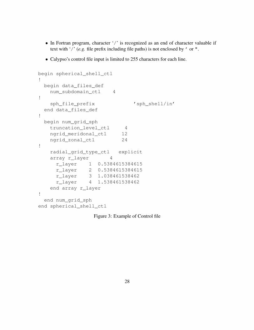
• In Fortran program, character ‘/’ is recognized as an end of character valuable iftext with ‘/’ (e.g. file prefix including file paths) is not enclosed by ’ or ".

• Calypso’s control file input is limited to 255 characters for each line.

begin spherical_shell_ctl!

begin data_files_defnum_subdomain_ctl 4

!sph_file_prefix ’sph_shell/in’

end data_files_def!

begin num_grid_sphtruncation_level_ctl 4ngrid_meridonal_ctl 12ngrid_zonal_ctl 24

!radial_grid_type_ctl explicitarray r_layer 4

r_layer 1 0.5384615384615r_layer 2 0.5384615384615r_layer 3 1.038461538462r_layer 4 1.538461538462

end array r_layer!

end num_grid_sphend spherical_shell_ctl

Figure 3: Example of Control file

28

8 ExamplesSeveral examples are provided in the examples directory. There are three subdirecto-ries as examples. README files are also provided to perform these examples in eachsubdirectory.

assemble sph Examples for assembling program of spectrum data. (see section 15)

dynamo benchmark Examples for dynamo benchmark by Christensen et. al. (2001)

heat composition source Examples for the heat and composition diffusion prob-lem including source term )

heterogineous temp Examples for the heat and composition diffusion problem in-cluding thermal and compositional heterogeneity at boundaries.)

spherical shell Examples for preprocessing program (see Section 9)

8.1 Examples for preprocessing programFour examples illustrate the use of the preprocessing program. The examples include

Chebyshev points Example to generate indexing data using Chebyshev collocationpoints

equidistance Example to generate indexing data with equi-distance grid

explicitly defined Example to generate indexing data with explicitly defined ra-dial points

with inner core Example to generate indexing data including inner core and exter-nal of the fluid shell.

The program gen_sph_grids generate spherical harmonics indexing file under thedirectory defined by the file control_sph_shell.

8.2 Examples of dynamo benchmarkThere are four examples for simulations using dynamo benchmark test as following.

Case 0 Example of dynamo benchmark case 0 (Thermally driven convection withoutmagnetic field)

29

Case 1 Example of dynamo benchmark case 1 (Dynamo model with co-rotating andelectrically insulated inner core)

Case 2 Example of dynamo benchmark case 2 (Dynamo model with rotatable and con-ductive inner core)

Compositional case 1 Example of dynamo benchmark case 1 using compositionalvariation instead of temperature

The process of the simulation in these examples is the same using 4 MPI processes:

1. Change to the directory for Benchmark Case 1 (for example)

[username]$ cd [CALYPSO_DIR]/examples/dynamo_benchmark/dynamobench_case1

2. Create the grid files for the simulation

[dynamobench_case_1]$ [CALYPSO_DIR]/bin/gen_sph_grids

3. Create initial field (Benchmark Case 1 only, see section 12)

[dynamobench_case_1]$ [CALYPSO_DIR]/bin/sph_initial_field

4. Run simulation program

[dynamobench_case_1]$ mpirun -np 4 [CALYPSO_DIR]/bin/sph_mhd

5. To continue the simulation, change the parameter rst_ctl in control_MHDfrom dynamo_benchmark_1 to start_from_rst_file and continue sim-ulation by repeating step 2.

6. To check the results for dynamo benchmark, run

[dynamobench_case_1]$ mpirun -np 4 [CALYPSO_DIR]/bin/sph_dynamobench

Each example has the following input and data outputs.

30

8.2.1 Data files and directories for Case 0

control sph shell Control file for spherical shell preprocessing

control MHD Control file for simulation

control snapshot Control file for postprocessing

sph lm31r48c 4 Spherical shell indexing data directory

rst 4 Spectr data directory for restarting

field Field data directory for for visualization

setions Cross section data directory for for visualization





control psf CMB Control file for section at CMB (See Section 10.5)

control psf eq Control file for section at equatorial plane (See Section 10.5)

control psf z0.3 Control file for section at z = 0.3 (See Section 10.5)

control psf s0.55 Control file for cylindrical surface at s = 0.55 (See Section 10.5)

control iso temp Control file for isosurface of temperature (See Section 10.6)





setions Cross section data directory for for visualization (See Section 10.5)

isourfaces Isosurface data directory for for visualization (See Section 10.6)

After running the program, the following files are written.

sph pwr volume s.dat Mean square data over the fluid shell.

31





control psf CMB Control file for section at CMB (See Section 10.5)

control psf ICB Control file for section at ICB (See Section 10.5)

control psf eq Control file for section at equatorial plane (See Section 10.5)

control psf z0.3 Control file for section at z = 0.3 (See Section 10.5)

control psf s0.55 Control file for cylindrical surface at s = 0.55 (See Section 10.5)




setions Cross section data directory for for visualization (See Section 10.5)

After running the program, the following files are written.

sph pwr volume s.dat Mean square data over the fluid shell.

8.2.4 Data files and directories for Compositional Case 1

const sph initial spectr.f90 Source code to generate initial field (need )







32

8.3 Example of data assembling programAn example for spectrum data assembling program is provided in assemble_sph di-rectory. This example uses simulation results of dynamo benchmark case 1. First, copydata from dynamo benchmark case 1 as

[assemble_sph]$ cp ../dynamo_benchmark/dynamobench_case_1/sph_lm31r48c_4/* sph_lm31r48c_4/[assemble_sph]$ cp ../dynamo_benchmark/dynamobench_case_1/rst_4/rst.* 4domains/

Then, construct new domain decomposition data as

[sph_lm31r48c_4]$ sph_lm31r48c_2[sph_lm31r48c_2]$ [CALYPSO_DIR]/bin/gen_sph_grids[sph_lm31r48c_2]$ cd ../

Finally restart data for new configuration is generated by assemble_sph in 2doaminsdirectory.

[sph_lm31r48c_2]$ [CALYPSO_DIR]/bin/assemble_sph

8.4 Example of treatment of heat and composition source termThis example solves heat and composition diffusion with including source terms. In thisexample, only temperature and composition are solved by

∂T

∂t= κT∇2T + qT ,

∂C

∂t= κC∇2C + qC ,

In the present example, diffusivities are fixed to be κT = κC = 1. Heat and compositionsources are given as qT = 2

rand qC = 1.0, respectively. The source terms are given in the

initial field data. The procedure of the simulation is the same as for the dynamo benchmarkCase 1. However, initial field generation program sph_initial_field is required tobuild by the following process:

1. Copy source file const_sph_initial_spectr.f90 to[CALYPSO_DIR]/src/programs/data_utilities/INITIAL_FIELD.

\verb|$[sph_initial_field]$ INITIAL_FIELD|

2. Build initial field generation program again.

33

[sph_initial_field]$ cd [CALYPSO_DIR]/work[work]$ make

3. Return to the example directory

[work]$ cd [CALYPSO]/examples/heat_composition_source

After building sph_initial_field, the procedure is the same as for the dynamobenchmarks. Aftrer the simulation, Y 0

0 component of temperature and composition as afunction of radius and time is written in picked_mode.dat.

8.5 Example of thermal and compositional boundary conditions byexternal file

Heterogeneous boundary are input using an external file. An example to set thermaland compositional boundary conditions is given in heterogineous_temp directory.As in the heat source example, only the diffusion problem is solved in this example.In file bc_spectr.btx, temperature boundary conditions are defined for Y 0

0 , Y 1s1 ,

Y 1c1 , and ,Y 2c

2 component, and compositional boundary is defined for Y 00 , Y 2s

2 , and Y 2c2

components. The radial profile of these spherical harmonics coefficients are written inpicked_mode.dat.

34

9 Preprocessing program (gen sph grid)

Simulation(sph_mhd)


FEM mesh data



(sph_zm_snapshot)

Spectr index data


Output data


Surface data(VTK)

Figure 4: Generated files by preprocessing program in Data flow.

This program generates index table and a communication table for parallel sphericalharmonics, table of integrals for Coriolis term, and FEM mesh information to generatevisualization data (see Figure 4). This program needs control file for input. This programcan perform with any number of MPI processes less than the number of subdomains. Theoutput files include the indexing tables.

Table 2: List of files for gen sph grid

extension Parallelization I/Ocontrol_sph_grid Single Input

[sph_prefix].[domain#].rj Distributed Output[sph_prefix].[domain#].rlm Distributed Output[sph_prefix].[domain#].rtm Distributed Output[sph_prefix].[domain#].rtp Distributed Output[sph_prefix].[domain#].gfm Distributed Output

radial_info.dat Single Output

35

9.1 Position of radial gridThe preprocessing program sets the radial grid spacing, either by a list in the control fileor by setting an equidistant grid or Chebyshev collocation points.

In equidistance grid, radial grids are defined by

r(k) = ri + (ro − ri)k − kICB

N,

where, kICB is the grid points number at ICB. The radial grid set from the closest pointsof minimum radius defined by [Min radius ctl] in control file to the closest pointsof the maximum radius defined by [Max radius ctl] in control file, and radial gridnumber for the innermost points is set to k = 1.

In Chebyshev collocation points, radial grids in the fluid shell are defined by

r(k) = ri +(ro − ri)

2

[1

2− cos

(πk − kICB

N

)],

For the inner core (r < ri), grid points is defined by

r(k) = ri −(ro − ri)

2

[1

2− cos

(πk − kICB

N

)],

and, grid points in the external of the shell (r > ro) is defined by

r(k) = ro +(ro − ri)

2

[1

2− cos

(πk − kCMB

N

)],

where, kCMB is the grid point number at CMB.

9.2 Control file (control sph shell)

Control files for Calypso consists of blocks starting and ending with begin and end, re-spectively. Entities with more than one components are defined between begin arrayand end array flags. The number of components of an array must be defined at begin arrayline. If blocks to be defined in an external file, the external file name is defined by fileflag.

Control file (control sph shell) consists the following items. Detailed descrip-tion for each item can be checked by clicking ”(Detail)” at the end of each item.spherical_shell_ctl

36

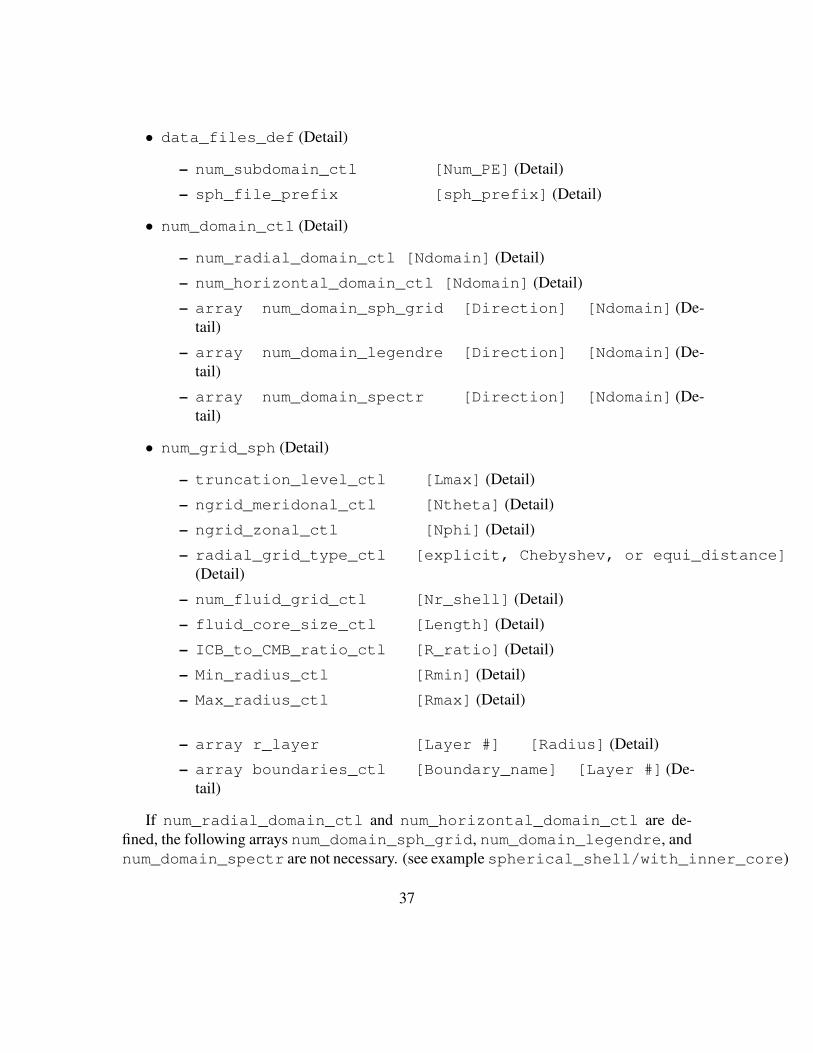
• data_files_def (Detail)

– num_subdomain_ctl [Num_PE] (Detail)

– sph_file_prefix [sph_prefix] (Detail)

• num_domain_ctl (Detail)

– num_radial_domain_ctl [Ndomain] (Detail)

– num_horizontal_domain_ctl [Ndomain] (Detail)

– array num_domain_sph_grid [Direction] [Ndomain] (De-tail)

– array num_domain_legendre [Direction] [Ndomain] (De-tail)

– array num_domain_spectr [Direction] [Ndomain] (De-tail)

• num_grid_sph (Detail)

– truncation_level_ctl [Lmax] (Detail)

– ngrid_meridonal_ctl [Ntheta] (Detail)

– ngrid_zonal_ctl [Nphi] (Detail)

– radial_grid_type_ctl [explicit, Chebyshev, or equi_distance](Detail)

– num_fluid_grid_ctl [Nr_shell] (Detail)

– fluid_core_size_ctl [Length] (Detail)

– ICB_to_CMB_ratio_ctl [R_ratio] (Detail)

– Min_radius_ctl [Rmin] (Detail)

– Max_radius_ctl [Rmax] (Detail)

– array r_layer [Layer #] [Radius] (Detail)

– array boundaries_ctl [Boundary_name] [Layer #] (De-tail)

If num_radial_domain_ctl and num_horizontal_domain_ctl are de-fined, the following arrays num_domain_sph_grid, num_domain_legendre, andnum_domain_spectr are not necessary. (see example spherical_shell/with_inner_core)

37

9.3 Spectrum index datagen_sph_grid generates indexing table of the spherical transform. To perform spheri-cal harmonics transform with distributed memory computers, data communication table isalso included in these files. Calypso needs four indexing data for the spherical transform.

[sph_prefix].[domain#].rj Indexing table for spectrum data f(r, l,m) to cal-culate linear terms. In program, spherical harmonics modes (l,m) is indexed byj = l(l+1)+m. The spectrum data are decomposed by spherical harmonics modesj. Data communication table for Legendre transform is included. The data also havethe radial index of the ICB and CMB.

[sph_prefix].[domain#].rlm Indexing table for spectrum data f(r, l,m) forLegendre transform. The spectrum data are decomposed by radial direction r andspherical harmonics order m. Data communication table to caricurate liner terms isincluded.

[sph_prefix].[domain#].rtm Indexing table for data f(r, θ,m) for Legendretransform. The data are decomposed by radial direction r and spherical harmonicsorder m. Data communication table for backward Fourier transform is included.

[sph_prefix].[domain#].rtp Indexing table for data f(r, θ,m) for Fourier trans-form and field data f(r, θ, φ). The data are decomposed by radial direction r andmeridional direction θ. Data communication table for forward Legendre transformis included.

9.4 Finite element mesh dataCalypso generates field data for visualization with XDMF or VTK format. To generatefield data file, the preprocessing program generates FEM mesh data for each subdomain ofspherical grid (r, θ, φ) under the Cartesian coordinate (x, y, z). The mesh data file is writ-ten as GeoFEM (http://geofem.tokyo.rist.or.jp) mesh data format, whichconsists of each subdomain mesh and communication table among overlapped nodes.

9.5 Radial grid dataThe preprocessing program generates radius of each layer in radial_info.dat ifradial_grid_type_ctl is set to Chebyshev or equi_distance. This file con-sists of blocks array r_layer and array boundaries_ctl for control file. Thisdata may be useful if you want to modify radial grid spacing by yourself.

38

http://geofem.tokyo.rist.or.jp

9.6 How to define spatial resolution and parallelization?Calypso uses spherical harmonics expansion method and in horizontal discretization andfinite difference methods in the radial direction. In the spherical harmonics expansionmethods, nonlinear terms are solved in the grid space while time integration and dif-fusion terms are solved in the spectrum space. We need to set truncation degree lmaxof the spherical harmonics and number of grids in the three direction (Nr, Nθ, Nφ) inthe preprocessing program. The following condition is required (or recommended) forlmax and (Nr, Nθ, Nφ). lmax is defined by truncation_level_ctl, and Nr for thefluid shell (outer core) is defined by num_fluid_grid_ctl. Nθ and Nφ is defined byngrid_meridonal_ctl and ngrid_zonal_ctl, respectively.

• Nφ = 2Nθ.

• Nθ must be more than lmax + 1, but

• To eliminate aliasing in the spherical transform, Nθ ≥ 1.5 (lmax + 1) is highly rec-ommended.

• Nφ should consists of products among power of 2, power of 3, and power of 5.

Calypso is parallelized 2-dimensionally and direction of the parallelization is changed inthe operations in the spherical transform (See Figure 5). Two dimensional paralleliza-tion delivers many parallelize configuration. Here is the approach how to find the bestconfiguration:

• Maximum parallelization level in horizontal direction is (lmax + 1) /2, and Nr + 1is the maximum level in radial direction.

• Decompose number of radial points Nr + 1 and truncation degree (lmax + 1) /2 intoprime numbers.

• Decide number of MPI processes from the prime numbers.

• Choose the number of decomposition in the radial and horizontal direction as closeas possible.

Here is an example for the case with (Nr, lmax) = (89, 95). The maximum number ofparallelization is 90× 48 = 4320 processes. Nr + 1 and (lmax + 1) /2 can be decomposedinto 90 = 2×32×5 and 48 = 24×3. Now, if 160 processes run is intended, 160 = 10×16is the closest number of decompositions. Comparing with the prime numbers of the spatialresolution, radial and horizontal decomposition will be 10 and 16, respectively.

39

Communication

Communication

Legendre transform

θθ

Spectrum datafor time integration

Grid space datafor nonlinear terms

Figure 5: Parallelization and data communication in Calypso in the case using 9 (3x3)processors. Data are decomposed in radial and meridional direction for nonlinear termevaluations, decomposed in radial and harmonic order for Legendre transform, and de-composed in spherical harmonics for linear calculations.

40

10 Simulation program (sph mhd)The name of the simulation program is sph mhd. This program requires control MHDas a Control file. This program performs with the indexing file for spherical harmonics andCoriolis term integration file generated by the preprocessing program gen sph grid.Data files for this program are listed in Table 3. Indexing data for spherical harmonics

Simulation(sph_mhd)


FEM mesh data



(sph_zm_snapshot)

Spectr index data


Output data


Surface data(VTK)

Figure 6: Data flow for the simulation program.

which starting with [sph_prefix] are obtained by the preprocessing program gen_sph_grid.The boundary condition data file [boundary_data_name] is optionally required ifboundary conditions for temperature and composition are not homogenous.

41

Table 3: List of files for simulation sph mhd

name Parallelization I/Ocontrol_MHD Serial Input

[sph_prefix].[domain#].rj Distributed Input[sph_prefix].[domain#].rlm Distributed Input[sph_prefix].[domain#].rtm Distributed Input[sph_prefix].[domain#].rtp Distributed Input[sph_prefix].[domain#].gfm Distributed Input

[boundary_data_name] Single Input[rst_prefix].[step#].[domain#].fst Distributed Input/Output

[vol_pwr_prefix]_s.dat Single Output[vol_pwr_prefix]_l.dat Single Output[vol_pwr_prefix]_m.dat Single Output[vol_pwr_prefix]_lm.dat Single Output[vol_ave_prefix].dat Single Output

[layer_pwr_prefix]_s.dat Single Output[layer_pwr_prefix]_l.dat Single Output[layer_pwr_prefix]_m.dat Single Output[layer_pwr_prefix]_lm.dat Single Output[gauss_coef_prefix].dat Single Output[picked_sph_prefix].dat Single Output

[nusselt_number_prefix].dat Single Output[fld_prefix].[step#].[domain#].[extension] - Output

[section_prefix].[step#].[extension] Single Output[isosurface_prefix].[step#].[extension] Single Output

42

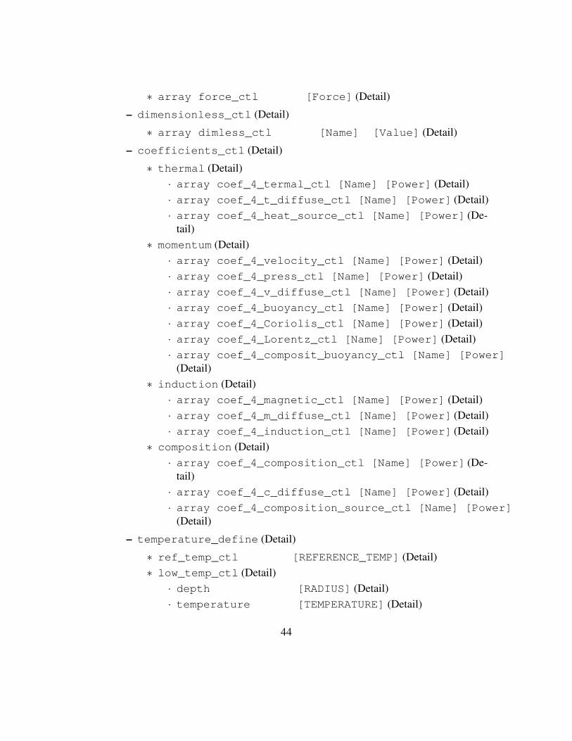
10.1 Control fileThe format of the control file control_MHD is described below. The detail of each blockis described in section A. You can jump to detailed description by clicking ”(Detail)”.

MHD_control (Header of the control file)



– num_smp_ctl [Num_Threads] (Detail)


– boundary_data_file_name [boundary_data_name] (De-tail)

– restart_file_prefix [rst_prefix] (Detail)

– field_file_prefix [fld_prefix] (Detail)

– field_file_fmt_ctl [fld_format] (Detail)

• model

– phys_values_ctl (Detail)

∗ array nod_value_ctl [Field] [Viz_flag] [Monitor_flag](Detail)

– time_evolution_ctl (Detail)

∗ array time_evo_ctl [Field] (Detail)

– boundary_condition (Detail)

∗ array bc_temperature [Group] [Type] [Value](Detail)∗ array bc_velocity [Group] [Type] [Value]

(Detail)∗ array bc_composition [Group] [Type] [Value]

(Detail)∗ array bc_magnetic_field [Group] [Type] [Value]

(Detail)

– forces_define (Detail)

43

∗ array force_ctl [Force] (Detail)

– dimensionless_ctl (Detail)

∗ array dimless_ctl [Name] [Value] (Detail)

– coefficients_ctl (Detail)

∗ thermal (Detail)· array coef_4_termal_ctl [Name] [Power] (Detail)· array coef_4_t_diffuse_ctl [Name] [Power] (Detail)· array coef_4_heat_source_ctl [Name] [Power] (De-

tail)∗ momentum (Detail)· array coef_4_velocity_ctl [Name] [Power] (Detail)· array coef_4_press_ctl [Name] [Power] (Detail)· array coef_4_v_diffuse_ctl [Name] [Power] (Detail)· array coef_4_buoyancy_ctl [Name] [Power] (Detail)· array coef_4_Coriolis_ctl [Name] [Power] (Detail)· array coef_4_Lorentz_ctl [Name] [Power] (Detail)· array coef_4_composit_buoyancy_ctl [Name] [Power]

(Detail)∗ induction (Detail)· array coef_4_magnetic_ctl [Name] [Power] (Detail)· array coef_4_m_diffuse_ctl [Name] [Power] (Detail)· array coef_4_induction_ctl [Name] [Power] (Detail)

∗ composition (Detail)· array coef_4_composition_ctl [Name] [Power] (De-

tail)· array coef_4_c_diffuse_ctl [Name] [Power] (Detail)· array coef_4_composition_source_ctl [Name] [Power]

(Detail)

– temperature_define (Detail)

∗ ref_temp_ctl [REFERENCE_TEMP] (Detail)∗ low_temp_ctl (Detail)· depth [RADIUS] (Detail)· temperature [TEMPERATURE] (Detail)

44

∗ high_temp_ctl (Detail)· depth [RADIUS] (Detail)· temperature [TEMPERATURE] (Detail)

• control

– time_step_ctl (Detail)

∗ elapsed_time_ctl [ELAPSED_TIME] (Detail)∗ i_step_init_ctl [ISTEP_START] (Detail)∗ i_step_finish_ctl [ISTEP_FINISH] (Detail)∗ i_step_check_ctl [ISTEP_MONITOR] (Detail)∗ i_step_rst_ctl [ISTEP_RESTART] (Detail)∗ i_step_field_ctl [ISTEP_FIELD] (Detail)∗ i_step_sectioning_ctl [ISTEP_SECTION] (Detail)∗ i_step_isosurface_ctl [ISTEP_ISOSURFACE] (Detail)∗ dt_ctl [DELTA_TIME] (Detail)∗ time_init_ctl [INITIAL_TIME] (Detail)

– restart_file_ctl (Detail)

∗ rst_ctl [INITIAL_TYPE] (Detail)

– time_loop_ctl (Detail)

∗ scheme_ctl [EVOLUTION_SCHEME] (Detail)∗ coef_imp_v_ctl [COEF_INP_U] (Detail)∗ coef_imp_t_ctl [COEF_INP_T] (Detail)∗ coef_imp_b_ctl [COEF_INP_B] (Detail)∗ coef_imp_c_ctl [COEF_INP_C] (Detail)∗ FFT_library_ctl [FFT_Name] (Detail)∗ Legendre_trans_loop_ctl [Leg_Loop] (Detail)

• sph_monitor_ctl (Detail)

– volume_average_prefix [vol_ave_prefix] (De-tail)

– volume_pwr_spectr_prefix [vol_pwr_prefix] (De-tail)

45

– layered_pwr_spectr_prefix [layer_pwr_prefix](Detail)

– picked_sph_prefix [picked_sph_prefix](Detail)

– gauss_coefs_prefix [gauss_coef_prefix](Detail)

– gauss_coefs_radius_ctl [gauss_coef_radius](Detail)

– nusselt_number_prefix [nusselt_number_prefix](Detail)

– array pick_layer_ctl [Layer #] (Detail)

– array pick_sph_spectr_ctl [Degree] [Order](Detail)

– array pick_sph_degree_ctl [Degree] (Detail)

– array pick_sph_order_ctl [Order] (Detail)

– array pick_gauss_coefs_ctl [Degree] [Order](Detail)

– array pick_gauss_coef_degree_ctl [Degree] (Detail)

– array pick_gauss_coef_order_ctl [Order] (Detail)

– nphi_mid_eq_ctl [Nphi_mid_equator] (Detail)

• visual_control (Detail)

– array cross_section_ctl [File or Block] (Detail)

– array isosurface_ctl [File or Block] (Detail)

10.2 Spectrum data for restartingSpectrum data is used for restarting data and generating field data by Data transform pro-gram sph_snapshot, sph_zm_snapshot, or sph_dynamobench. This file issaved for each subdomain (MPI processes), then [step #] and [domain #] are addedin the file name. The [step #] is calculated by time step / [ISTEP_RESTART].

46

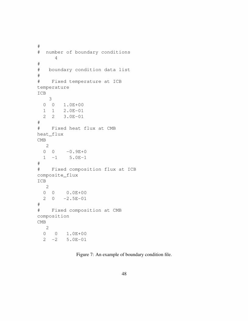
10.3 Thermal and compositional boundary condition data fileThermal and compositional heterogeneity at boundaries are defined by a external filenamed [boundary_data_name]. In this file, temperature, composition, heat flux,or compositional flux at ICB or CMB can be defined by spherical harmonics coeffi-cients. To use boundary conditions in [boundary_data_name], file name is de-fined by boundary_data_file_name column in control file, and boundary conditiontype [type] is set to fixed_file or fixed_flux_file in bc_temperature orbc_composition column. By setting fixed_file or fixed_flux_file in con-trol file, boundary conditions are copied from the file [boundary_data_name].

An example of the boundary condition file is shown in Figure 7. As for the control file,a line starting from ’#’ or ’!’ is recognized as a comment line. In [boundary_data_name],boundary condition data is defined as following:

1. Number of total boundary conditions to be defined in this file.

2. Field name to define the first boundary condition

3. Place to define the first boundary condition (ICB or CMB)

4. Number of spherical harmonics modes for each boundary condition

5. Spectrum data for the boundary conditions (degree l, order m, and harmonics coef-ficients)

6. After finishing the list of spectrum data return to Step 2 for the next boundary con-dition

If harmonics coefficients of the boundary conditions are not listed in item 5, 0.0 is au-tomatically applied for the harmonics coefficients of the boundary conditions. So, onlynon-zero components need to be listed in the boundary condition file.

10.4 Field data for visualizationField data is used for the visualization processes. Field data are written with XDMF format(http://www.xdmf.org/index.php/Main_Page), merged VTK, or distributedVTK format (http://www.vtk.org/VTK/img/file-formats.pdf). The out-put data format is defined by fld_format. Visualization applications which we checkedare listed in Table 4. Because the field data is written by using Cartesian coordinate(x, y, z) system, coordinate conversion is required to plot vector field in spherical coor-dinate (r, θ, φ) or cylindrical coordinate (s, φ, z). We will introduce a example of visual-ization process using ParaView in Section 18.

47

http://www.xdmf.org/index.php/Main_Page

http://www.vtk.org/VTK/img/file-formats.pdf

## number of boundary conditions

4## boundary condition data list## Fixed temperature at ICBtemperatureICB

30 0 1.0E+001 1 2.0E-012 2 3.0E-01

## Fixed heat flux at CMBheat_fluxCMB

20 0 -0.9E+01 -1 5.0E-1

## Fixed composition flux at ICBcomposite_fluxICB

20 0 0.0E+002 0 -2.5E-01

## Fixed composition at CMBcompositionCMB

20 0 1.0E+002 -2 5.0E-01

Figure 7: An example of boundary condition file.

48

Table 4: Checked visualization application

Format ApplicationDistributed VTK ParaView (http://www.paraview.org)

Merged VTK ParaView, VisIt (https://wci.llnl.gov/codes/visit/)Mayavi (http://mayavi.sourceforge.net/)

XDMF ParaView, VisIt

10.4.1 Distributed VTK data

Distributed VTK data have the following advantage and disadvantages to use:

• Advantage

– Faster output

– No external library is required

• Disadvantage

– Many data files are generated

– Total data file size is large

– Only ParaView supports this format

Distributed VTK data consist files listed in Table 5. For ParaView, all subdomain data isread by choosing [fld_prefix].[step#].pvtk in file menu.

Table 5: List of written files for distributed VTK format

name[fld_prefix].[step#].[domain#].vtk VTK data for each subdomain

[fld_prefix].[step#].pvtk Subdomain file list for Paraview

10.4.2 Merged VTK data

Merged VTK data have the following advantage and disadvantages to use:

49

http://www.paraview.org

https://wci.llnl.gov/codes/visit/

http://mayavi.sourceforge.net/

• Advantage

– Merged field data is generated

– No external library is required

– Many applications support VTK format

• Disadvantage

– Very slow to output

– Total data file size is large

Merged VTK data generate files listed in Table 6.

Table 6: List of written files for merged VTK format

name[fld_prefix].[step#].vtk Merged VTK data

10.4.3 Merged XDMF data

Merged XDMF data have the following advantage and disadvantages to use:

• Advantage

– Fastest output

– Merged field data is generated

– File size is smaller than the VTK formats

• Disadvantage

– Parallel HDF5 library should be required to use

Merged XDMF data generate files listed in Table 7. For ParaView, all subdomain data isread by choosing [fld_prefix].solution.xdmf in file menu.

50

Table 7: List of written files for XDMF format

name[fld_prefix].mesh.h5 HDF5 file for geometry data

[fld_prefix].[step#].h5 HDF5 file for field data[fld_prefix].solution.xdmf HDF5 file lists to be read

10.5 Cross section data (Parallel Surfacing moduleCalypso can output cross section data for visualization with finer time increment than thewhole domain data. The cross section data consist of triangle patches with VTK format,then data can be visualized by Paraview like as the whole field data. This cross sectioningmodule can output arbitrary quadrature surface, but plane, sphere, and cylindrical sectionwould be useful for the geodynamo simulations.

To output cross sectioning, increment of the surface output data should be defined byi_step_sectioning_ctl in time_step_ctl block. And, array blockcross_section_ctl in visual_control section is required to define cross sec-tions. Each cross_section_ctl block defines one cross section. Each cross sectioncan also define by an external file by specifying external file name with file label. Thesections shown in Table 8 are supported in the sectioning module. These surfaces aredefined in the Cartesian coordinate. The easiest approarch is using sections defined by

Table 8: Supported cross sections

Surface type equationQuadrature surface ax2 + by2 + cz2 + dyz + ezx+ fxy + gx+ hy + jz + k = 0

Plane surface a (x− x0) + b (y − y0) + c (z − z0) = 0

Sphere (x− x0)2 + (y − y0)2 + (z − z0)2 = r2

Ellipsoid(x− x0a

)2

+

(y − y0b

)2

+

(z − z0c

)2

= 1

quadrature function with ten coefficients from a to k in the control array coefs_ctl.A plane surface is defined by a normal vector (a, b, c) and one point including the

surface (x0, y0, z0) in arrays normal_vector and center_position, respectively.A sphere surface is defined by the position of the center (x0, y0, z0) and radius r in

array center_position and radius, respectively.

51

An Ellipsoid surface is defined the position of the center (x0, y0, z0) and length of theeach axis (a, b, c) in arrays center_position and axial_length, respectively. Ifone component of the axial_length is set to 0, surfacing module generate a Ellipsoidaltube along with the axis where axial_length is set to 0.

Area for visualization can be defined by array chosen_ele_grp_ctl by choosingouter_core, inner_core, and all. Fields to display is defined in array output_field.In array output_field, field type in Table 9 needs to defined. The same field can bedefined more than once in array output_field to output vector field in Cartesian co-ordinate and radial component, for example.

Table 9: List of field type for cross sectioning and isosurface module

Definition Field typescalar scalar fieldvector Cartesian vector field

x x-componenty y-componentz z-component

radial radial (r-) componenttheta θ-componentphi φ-component

cylinder_r cylindrical radial (s-) componentmagnitude magnitude of vector

10.5.1 Control file

The format of the control file or block for cross sections is described below. The detail ofeach block is described in section A. cross_section_ctl block can be read from anexternal file. To define the external file name, as file cross_section_ctl [file name]in control_MHD or control_snapshot. You can jump to detailed description byclicking ”(Detail)”.

cross_section_ctl (Header of the control file)

• section_file_prefix [section_prefix] (Detail)

• surface_define (Detail)

52

– section_method [METHOD] (Detail)

– array coefs_ctl [TERM] [COEFFICIENT] (Detail)

– radius [SIZE] (Detail)

– array normal_vector [DIRECTION] [COMPONENT] (Detail)

– array axial_length [DIRECTION] [COMPONENT] (Detail)

– array center_position [DIRECTION] [COMPONENT] (Detail)

– array section_area_ctl [AREA_NAME] (Detail)

• output_field_define (Detail)

– array output_field [FIELD] [COMPONENT] (Detail)

10.6 Isosurface dataCalypso can also output isosurface data for visualization. Generally, data size of the iso-surface is much larger than the sectioning data. The isosurface data is also written as aunstructured grid data with VTK format. The isosurface also consists of triangle patches.

To output cross sectioning, increment of the surface output data should be defined byi_step_isosurface_ctl in time_step_ctl block. And, array block isosurface_ctlin visual_control section is required to define cross sections. Each isosurface_ctlblock defines one cross section. Each cross section can also define by an external file byspecifying external file name with file label.

10.6.1 Control file

The format of the control file or block for isosurfaces is described below. The detail ofeach block is described in section A. isosurface_ctl block can be read from an exter-nal file. To define the external file name, as file isosurface_ctl [file name]in control_MHD or control_snapshot. You can jump to detailed description byclicking ”(Detail)”.

isosurface_ctl (Header of the control file)

• isosurface_file_prefix [file_prefix] (Detail)

• isosurf_define (Detail)

– isosurf_field [FIELD] (Detail)

53

– isosurf_component [COMPONENT] (Detail)

– isosurf_value [VALUE] (Detail)

– array isosurf_area_ctl [AREA_NAME] (Detail)

• field_on_isosurf (Detail)

– result_type [TYPE] (Detail)

– result_value [VALUE] (Detail)

– array output_field [FIELD] [COMPONENT] (Detail)

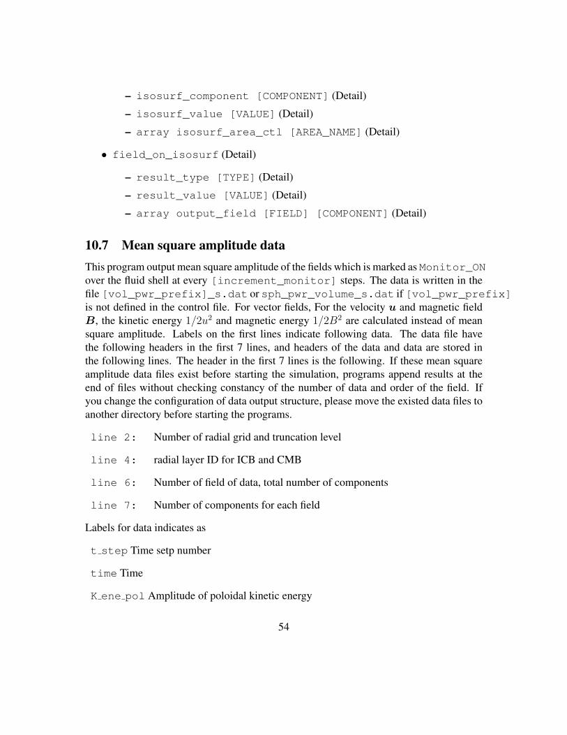
10.7 Mean square amplitude dataThis program output mean square amplitude of the fields which is marked as Monitor_ONover the fluid shell at every [increment_monitor] steps. The data is written in thefile [vol_pwr_prefix]_s.dat or sph_pwr_volume_s.dat if [vol_pwr_prefix]is not defined in the control file. For vector fields, For the velocity u and magnetic fieldB, the kinetic energy 1/2u2 and magnetic energy 1/2B2 are calculated instead of meansquare amplitude. Labels on the first lines indicate following data. The data file havethe following headers in the first 7 lines, and headers of the data and data are stored inthe following lines. The header in the first 7 lines is the following. If these mean squareamplitude data files exist before starting the simulation, programs append results at theend of files without checking constancy of the number of data and order of the field. Ifyou change the configuration of data output structure, please move the existed data files toanother directory before starting the programs.

line 2: Number of radial grid and truncation level

line 4: radial layer ID for ICB and CMB

line 6: Number of field of data, total number of components

line 7: Number of components for each field

Labels for data indicates as

t step Time setp number

time Time

K ene pol Amplitude of poloidal kinetic energy

54

K ene tor Amplitude of toroidal kinetic energy

K ene Amplitude of total kinetic energy

M ene pol Amplitude of poloidal magnetic energy

M ene tor Amplitude of toroidal magnetic energy

M ene Amplitude of total magnetic energy

[Field] pol Mean square amplitude of poloidal component of [Field]

[Field] tor Mean square amplitude of toroidal component of [Field]

[Field] Mean square amplitude of [Field]

10.7.1 Volume average data

Volume average data are written by defining volume average prefix in control file.Volume average data are written in [vol_ave_prefix].dat with same format asRMS amplitude data. If you need the sphere average data for specific radial point, you canuse picked spectrum data for l = m = 0 at specific radius.

10.7.2 Volume spectrum data

Volume spectrum data are written by defining volume pwr spectr prefix in con-trol file. By defining volume pwr spectr prefix, following spectrum data averagedover the fluid shell is written. Data format is the same as the volume mean square data, butdegree l, order m, or meridional wave number l −m is added in the list of data.

[vol pwr prefix l.dat Volume average of mean square amplitude of the fields asa function of spherical harmonic degree l. For scalar field, the spectrum is

fsq(l) =1

V

m=l∑m=−l

∫(fml )2 dV.

For vector field, spectrum for the poloidal and toroidal components are written by

BSsq(l) =1

V

m=l∑m=−l

∫(B m

Sl )2 dV,

BTsq(l) =1

V

m=l∑m=−l

∫(B m

Tl )2 dV.

55

If the vector field F is not solenoidal (i.e. ∇ · F 6= 0), The poloidal component ofmean square data are included mean square field of the potential components as

FSsq(l) =1

V

m=l∑m=−l

∫ [(B m

Sl )2 + (−∇φ m

Fl )2] dV.

[vol pwr prefix] m.dat Volume average of mean square amplitude of the fieldsas a function of spherical harmonic order m. The zonal wave number is referred inthis spectrum data. For scalar field, the spectrum is

fsq(m) =1

V

l=m∑l=0

∫ [(fml )2 +

(f−ml

)2]dV.


BSsq(m) =1

V

l=m∑l=0

∫ [(B m

Sl )2 +

(B −mSl

)2]dV,

BTsq(m) =1

V

l=m∑l=0

∫ [(B m

Tl )2 +

(B −mTl

)2]dV.

[vol pwr prefix] lm.dat Volume average of mean square amplitude of the fieldsas a function of spherical harmonic order n = l − m. The wave number in thelatitude direction is referred in this spectrum data. For scalar field, the spectrum is

fsq(n) =1

V

l=l−n∑l=n

∫ [(f l−nl

)2+(f−l+nl

)2]dV.


BSsq(n) =1

V

l=l−n∑l=n

∫ [(B l−nSl

)2+(B −l+nSl

)2]dV,

BTsq(n) =1

V

l=l−n∑l=n

∫ [(B l−nT l

)2+(B −l+nT l

)2]dV.

56

10.7.3 layered spectrum data

Spectrum data for the each radial position are written by defining layered pwr spectr prefixin control file. By defining layered pwr spectr prefix, following spectrum dataaveraged over the fluid shell is written. Data format is the same as the volume spectrumdata, but radial grid point and radius of the layer is added in the list. The following filesare generated. The radial points for output is listed in the array spectr_layer_ctl. Ifspectr_layer_ctl is not defined, mean square data at all radial levels will be written.See example of dynamo benchmark case 2.

[layer pwr prefix] s.dat Surface average of mean square amplitude of the fields.

[layer pwr prefix] l.dat Surface average of mean square amplitude of the fieldsas a function of spherical harmonic degree l and radial grid id k. For scalar field, thespectrum is

fsq(k, l) =1

S

m=l∑m=−l

∫(fml )2 dS.


BSsq(k, l) =1

S

m=l∑m=−l

∫(B m

Sl )2 dS,

BTsq(k, l) =1

S

m=l∑m=−l

∫(B m

Tl )2 dS.

[layer pwr prefix] m.dat Surace average of mean square amplitude of the fieldsas a function of spherical harmonic order m and radial grid id k. The zonal wavenumber is referred in this spectrum data. For scalar field, the spectrum is

fsq(k,m) =1

S

l=L∑l=m

∫ [(fml )2 +

(f−ml

)2]dS.


BSsq(k,m) =1

S

l=L∑l=m

∫ [(B m

Sl )2 +

(B −mSl

)2]dS,

BTsq(k,m) =1

S

l=L∑l=m

∫ [(B m

Tl )2 +

(B −mTl

)2]dS.

57

[layer pwr prefix] lm.dat Surface average of mean square amplitude of thefields as a function of spherical harmonic order n = l − m and radial grid id k.The wave number in the latitude direction is referred in this spectrum data. Forscalar field, the spectrum is

fsq(k, n) =1

S

l=L∑l=n

∫ [(f l−nl

)2+(f−l+nl

)2]dS.


BSsq(k, n) =1

S

l=L∑l=n

∫ [(B l−nSl

)2+(B −l+nSl

)2]dS,

BTsq(k, n) =1

S

l=L∑l=n

∫ [(B l−nT l

)2+(B −l+nT l

)2]dS.

10.8 Gauss coefficient data [gauss coef prefix].dat

This program output selected Gauss coefficients of the magnetic field. Gauss coefficients isevaluated for radius defined by [gauss_coef_radius] every [increment_monitor]steps. Gauss coefficients are evaluated by using poloidal magnetic field at CMB B m

Sl (ro)and radius defined by [gauss_coef_radius] re as

gml =l

r2e

(rore

)lB mSl (ro),

hml =l

r2e

(rore

)lB −mSl (ro).

The data file has the following headers in the first three lines,

line 2: Number of saved Gauss coefficients and reference radius.

line 3: Labels of Gauss coefficients data.

The data consists of time step, time, and Gauss coefficients for each step in one line. If theGauss coefficients data file exist before starting the simulation, programs append Gausscoefficients at the end of files without checking constancy of the number of data and orderof the field. If you change the configuration of data output structure, please move the oldGauss coefficients file to another directory before starting the programs.

58

10.9 Spectrum monitor data [picked sph prefix].dat

This program outputs spherical harmonics coefficients at specified spherical harmonicsmodes and radial points in single text file. Spectrum data marked [Monitor_On] arewritten in our line for each spherical harmonics mode and radial point every[increment_monitor] steps. If the spectrum monitor data file exist before startingthe simulation, programs append spectrum data at the end of files without checking con-stancy of the number of data and order of the field. If you change the configuration of dataoutput structure, please move the old spectrum monitor file to another directory beforestarting the programs.

If a vector field F is not a solenoidal field, F is described by the spherical harmonicscoefficients of the poloidal F m

Sl , toroidal F mTl , and potential ϕml components as

F (r, θ, φ) = − 1

r2∂ϕ0

0

∂rr +

L∑l=1

l∑m=−l

[∇×∇× (F mSl r) +∇× (F m

Tl )−∇ (ϕml Yml )] .

In Calypso, the following coefficients are written for the non-solenoidal vector.

[field_name]_pol :

F mSl −

r2

l (l + 1)

∂ϕml∂r

for (l 6= 0)

−r2∂ϕ00

∂rfor (l = 0)

[field_name]_dpdr :

∂F m

Sl

∂r− ϕml for (l 6= 0)

0 for (l = 0)

[field_name]_tor : F mTl

10.10 Nusselt number data [nusselt number prefix].dat

CAUTION: Nusselt number is not evaluated if heat source is exsist. The Nusselt num-ber Nu at CMB and ICB is written for each step in one line. The Nusselt number isevaluated by

Nu =< ∂T/∂r >

∂Tdiff/∂r,

where, < ∂T/∂r > and Tdiff are the horizontal average of the temperature gradient atICB and CMB and diffusive temperature profile, respectively. Tdiff is evaluated without

59

heat source, as

Tdiff =roTo − riTiro − ri

+rori (Ti − To)

ro − ri1

r.

This diffusive temperature profile is for the case without heat source in the fluid. If simu-lation is performed including the heat source, this data file does not written. If the Nusseltnumber data file exist before starting the simulation, programs append spectrum data atthe end of files without checking constancy. If you change the configuration of data outputstructure, please move the old spectrum monitor file to another directory before startingthe programs.

60

11 Data transform program(sph snapshot and sph zm snapshot)

Simulation(sph_mhd)


FEM mesh data



(sph_zm_snapshot)

Spectr index data


Output data


Surface data(VTK)

Figure 8: Data flow for data transform program.

Simulation program outputs spectrum data as a whole field data. This program gen-erates field data from spectrum data for visualization. This program also can pick Gausscoefficients, mean square data over sphere or each surface from spectrum data as the sim-ulation program.

This program requires control file control_snapshot. File format of the controlfile is same as the control field for simulation control MHD.

The same files as the simulation program are read in this program, and field data aregenerated from the snapshots of spectrum data. The monitoring data for snapshots canalso be generated. [step #] is added in the file name, and the [step #] is calculatedby time step/[ISTEP_FIELD].

We recommend to output cross section data at y = 0 by using sectioning module (see10.5) for zonal mean snapshot program sph_zm_snapshot to reduce data size.

61

Table 10: List of files for simulation sph snap and sph zm snap

name Parallelization I/Ocontrol_snapshot Serial Input

[sph_prefix].[domain#].rj Distributed Input[sph_prefix].[domain#].rlm Distributed Input[sph_prefix].[domain#].rtm Distributed Input[sph_prefix].[domain#].rtp Distributed Input[sph_prefix].[domain#].gfm Distributed Input

[boundary_data_name] Single Input[rst_prefix].[step#].[domain#].fst Distributed Input

[vol_pwr_prefix].dat Single Output[vol_pwr_prefix]_l.dat Single Output[vol_pwr_prefix]_m.dat Single Output[vol_pwr_prefix]_lm.dat Single Output[vol_ave_prefix].dat Single Output

[layer_pwr_prefix]_l.dat Single Output[layer_pwr_prefix]_m.dat Single Output[layer_pwr_prefix]_lm.dat Single Output[gauss_coef_prefix].dat Single Output[picked_sph_prefix].dat Single Output

[nusselt_number_prefix].dat Single Output[fld_prefix].[step#].[domain#].[extension] - Output

62

12 Initial field generation program(sph initial field)

Initial eld(sph_initial_eld)


Spectr index data


Output data

Figure 9: Data flow for initial field generation program.

The initial fields for dynamo benchmark can set in the simulation program by setting[INITIAL_TYPE] flag. This program is used to generate initial field by user. The heatsource qT and light element source qC are also defined by this program because qT and qCare defined as scalar fields. The Fortran source file to define initial fieldconst_sph_initial_spectr.f90 is saved in src/programs/data_utilities/INITIAL_FIELD/ directory, and please compile again after modifying this module.This program also needs the files listed in Table 11. This program generates the spectrum

Table 11: List of files for simulation sph initial field


[sph_prefix].[domain#].rj Distributed Input[sph_prefix].[domain#].rlm Distributed Input[sph_prefix].[domain#].rtm Distributed Input[sph_prefix].[domain#].rtp Distributed Input[rst_prefix].0.[domain#].fst Distributed Input/Output

data files [rst_prefix].0.[domain#].fst. To use generated initial data file,

63

please set [ISTEP START] to be 0 and [INITIAL TYPE] to be start from rst file.

12.1 Definition of the initial fieldTo construct Initial field data, you need to edit the source code const_sph_initial_spectr.f90in src/programs/data_utilities/INITIAL_FIELD/ directory. The moduleconst_sph_initial_spectr consists of the following subroutines:

sph_initial_spectrum: Top subroutine to construct initial field.

set_initial_velocity: Routine to construct initial velocity.

set_initial_temperature: Routine to construct initial temperature.

set_initial_composition: Routine to construct initial composition.

set_initial_magne_sph: Routine to construct initial magnetic field.

set_initial_heat_source_sph: Routine to construct heat source.

set_initial_light_source_sph: Routine to construct composition source.

The construction routine for each field are called from the top routineconst_sph_initial_spectr.f90. If lines to call subroutines are commented out,corresponding initial fields are set to 0. In addition, the initial fields to be constructed needto be defined by nod_value_ctl array in the control_MHD.

Table 12: Field name and corresponding field id in Calypso

field name scalar poloidal toroidalVelocity - ipol%i_velo itor%i_velo

Magnetic field - ipol%i_magne itor%i_magneCurrent density - ipol%i_current itor%i_current

Temperature ipol%i_temp - -Composition ipol%i_light - -Heat source ipol%i_heat_source - -

Composition source ipol%i_light_source - -

64

Initial fields need to be defined by the spherical harmonics coefficients at each radialpoints as array d_rj(i,i_field), where i and i_field are the local address of thespectrum data and field id, respectively. The address of the fields are listed in Table 12.

In Calypso, local data address for each MPI process is used for the spectrum data ad-dress i. To find the local address i, two functions are required.First, j = find_local_sph_mode_address(l,m) returns the local spherical har-monics address j from aa spherical harmonics mode Y m

l . If process does not have thedata for Y m

l , j is set to 0. Second, i = local_sph_data_address(k,j) re-turns the local data address i from radial grid number k and local spherical harmonicsid j. For do loops in the radial direction, the total number of radial grid points, radial ad-dress for ICB, and radial address for CMB are defined as nidx_rj(1), nlayer_ICB,and nlayer_CMB, respectively. The radius for the k-th grid points can be obtained byr = radius_1d_rj_r(k). The subroutines to define initial temperature for the dy-namo benchmark Case 1 is shown below as an example.

After updating the source code, the program sph_initial_field needs to beupdated. To update the program, move to the work directory [CALYPSO_HOME]/workand run make command as

% cd \verb|[CALYPSO_HOME]/work|% make

Then, the program sph_initial_field and sph_add_initial_field are up-dated.

!subroutine set_initial_temperature

!use m_sph_spectr_data

!integer ( kind = kint) :: inod, k, jjreal (kind = kreal) :: pi, rr, xr, shellreal(kind = kreal), parameter :: A_temp = 0.1d0

!!!$omp parallel do

do inod = 1, nnod_rjd_rj(inod,ipol%i_temp) = zero

end do!$omp end parallel do

65

!pi = four * atan(one)shell = r_CMB - r_ICB

!! search address for (l = m = 0)

jj = find_local_sph_mode_address(0, 0)!! set reference temperature if (l = m = 0) mode is there

if (jj .gt. 0) thendo k = 1, nlayer_ICB-1inod = local_sph_data_address(k,jj)d_rj(inod,ipol%i_temp) = 1.0d0

end dodo k = nlayer_ICB, nlayer_CMBinod = local_sph_data_address(k,jj)d_rj(inod,ipol%i_temp) = (ar_1d_rj(k,1) * 20.d0/13.0d0 &

& - 1.0d0 ) * 7.0d0 / 13.0d0end do

end if!!! Find local addrtess for (l,m) = (4,4)

jj = find_local_sph_mode_address(4, 4)! jj = find_local_sph_mode_address(5, 5)!! If data for (l,m) = (4,4) is there, set initial temperature

if (jj .gt. 0) then! Set initial field from ICB to CMB

do k = nlayer_ICB, nlayer_CMB!! Set radius data

rr = radius_1d_rj_r(k)! Set 1d address to substitute at (Nr, j)

inod = local_sph_data_address(k,jj)!! set initial temperature

xr = two * rr - one * (r_CMB+r_ICB) / shelld_rj(inod,ipol%i_temp) = (one-three*xr**2+three*xr**4-xr**6) &

66

& * A_temp * three / (sqrt(two*pi))end do

end if!! Center

if(inod_rj_center .gt. 0) thenjj = find_local_sph_mode_address(0, 0)inod = local_sph_data_address(1,jj)d_rj(inod_rj_center,ipol%i_temp) = d_rj(inod,ipol%i_temp)

end if!

end subroutine set_initial_temperature!

13 Initial field modification program(sph add initial field)

Initial eld(sph_initial_eld)


Spectr index data


Output data

Figure 10: Data flow for initial field modification program.

Caution: This program overwrites existing initial field data. Please run it aftertaking a backup.

This program modifies or adds new data to an initial field file. It could be usedto start a new geodynamo simulation by adding seed magnetic field or source terms to

67

a non-magnetic convection simulation. The initial fields to be added are also definedin const_sph_initial_spectr.f90. data_utilities/INITIAL_FIELD/directory. This program also needs the files listed in Table 13. This program generates the

Table 13: List of files for simulation sph add initial field


[sph_prefix].[domain#].rj Distributed Input[sph_prefix].[domain#].rlm Distributed Input[sph_prefix].[domain#].rtm Distributed Input[sph_prefix].[domain#].rtp Distributed Input

[rst_prefix].[step #].[domain#].fst Distributed Input/Output

spectrum data files [rst_prefix].[step#].[domain#].fst. To use generatedinitial data file, set [ISTEP START] and [ISTEP_RESTART] to be appropriate timestep and increment, respectively. To read the original initial field data, [INITIAL TYPE]is set to be start from rst file in control_MHD. In other words, the [step #]in the file name, [ISTEP START], and [ISTEP_RESTART] in the control file shouldbe the consistent.

This program also uses the module file const_sph_initial_spectr.f90 todefine the initial field. The initial fields are defined as following the previous section12.1. After updating the source code, the program sph_initial_field needs to beupdated. After modifying const_sph_initial_spectr.f90, the program is buildby make command in the work directory [CALYPSO_HOME]/work.

14 Check program for dynamo benchmark(sph dynamobench)

This program is only used to check solution for dynamo benchmark by Christensen et. al.The following files are used for this program.

68

Table 14: List of files for dynamo benchmark check sph dynamobench

name Parallelization I/Ocontrol_snapshot Serial Input

[sph_prefix].[domain#].rj Distributed Input[sph_prefix].[domain#].rlm Distributed Input[sph_prefix].[domain#].rtm Distributed Input[sph_prefix].[domain#].rtp Distributed Input

[rst_prefix].[step#].[domain#].fst Distributed Inputdynamobench.dat Single Output

14.1 Dynamo benchmark data dynamobench.datIn benchmark test by Christensen et. al., both global values and local values are checked.

As global results, Kinetic energy1

V

∫1

2u2dV in the fluid shell, magnetic energy in

the fluid shell1

V

1

EPm

∫1

2B2dV (for case 1 and 2), and magnetic energy in the solid

inner sphere1

Vi

1

EPm

∫1

2B2dVi (for case 2 only). Benchmark also requests By in-

creasing number of grid point at mid-dpeth of the fluid shell in the equatorial plane bynphi mid eq ctl, program can find accurate solution for the point where ur = 0 and∂ur/∂φ > 0. Angular frequency of the field pattern with respect to the φ direction isalso required. The benchmark test also requires temperature and θ component of velocity.In the text file dynamobench.dat, the following data are written in one line for every[i_step_rst_ctl] step.

t step: Time step number

time: Time

KE pol: Poloidal kinetic energy

KE tor: Toroidal kinetic energy

KE total: Total kinetic energy

ME pol: Poloidal magnetic energy (Case 1 and 2)

ME tor: Toroidal magnetic energy (Case 1 and 2)

69

ME total: Total magnetic energy (Case 1 and 2)

ME pol ic: Poloidal magnetic energy in inner core (Case 2)

ME tor icore: Toroidal magnetic energy in inner core (Case 2)

ME total icore: Total magnetic energy in inner core (Case 2)

omega ic z: Angular velocity of inner core rotation (Case 2)

MAG torque ic z: Magnetic torque integrated over the inner core (Case 2)

phi 1...4: Longitude where ur = 0 and ∂ur/∂φ > 0 at mid-depth in equatorialplane.

omega vp44: Drift frequency evaluated by V 4S4 component

omega vt54: Drift frequency evaluated by V 4T5 component

B theta: Θ component of magnetic field at requested point.

v phi: φ component of velocity at requested point.

temp: Temperature at requested point.

t_step time KE_pol KE_tor KE_total ME_pol ME_tor ME_total ME_pol_icore ME_tor_icore ME_total_icore

omega_ic_z MAG_torque_ic_z phi_1 phi_2 phi_3phi_4 omega_vp44 omega_vt54 B_theta v_phi temp

20000 9.999999999998981E-001 1.534059732073072E+001 2.431439471284618E+001 3.965499203357688E+001 2.405694011955009E+000 1.648662987055900E+000 4.054356999010911E+000 3.908687924452961E+001 4.812865754441352E-001 3.956816581997376E+001 5.220517005592486E+000 -2.321885847438682E+002 3.594175626663308E-001 1.930213889461227E+000 3.501010216256124E+000 5.071806543051021E+000 7.808553595635292E-001 -1.649583441437563E-001 -5.136522824340612E+000 -8.047915942925034E+0003.752181234262930E-001...

70

Assemble(assemble_sph)


Spectr index data

Input data Program(Serial)

Output data

New spectrindex data


Figure 11: Data flow for spectrum data assemble program

15 Data assemble program (assemble sph)Calypso uses distributed data files for simulations. This program is to generate new spec-trum data for restarting with different spatial resolution or parallel configuration. This pro-gram organizes new spectral data by using specter indexing data using different domaindecomposition. The following files used for data IO. If radial resolution is changed fromthe original data, the program makes new spectrum data by linear interpolation. If new datahave smaller or larger truncation degree, the program fills zero to the new spectrum data ortruncates the data to fit the new spatial resolution, respectively. This program can performwith any number of MPI processes, but we recommend to run the program with one pro-cess or the same number of processes as the number of subdomains for the target configura-tion which is defined by num_new_domain_ctl. Data files for the program are shownIn Table 15. The time and number of time step can also be changed by this program. Thenew time and time step are defined by the parameters in new_time_step_ctl block.The step number of the restart data will be i_step_init_ctl / i_step_rst_ctlin new_time_step_ctl. If new_time_step_ctl block is not defined, time andtime step informations are carried from the original restart data.

15.1 Format of control fileControl file consists the following groups.assemble_control


71

Table 15: List of files for assemble sph

extension Distributed? I/Ocontrol_sph_assemble Serial Input

[sph_prefix].[domain#].rj Distributed Input[new_sph_prefix].[domain#].rj Distributed Input

[rst_prefix].[step#].[domain#].fst Distributed Input[new_rst_prefix].[step#].[domain#].fst Distributed Output



– restart_file_prefix [rst_prefix] (Detail)

• new_data_files_def (Detail)

– num_new_domain_ctl [new_num_domain] (Detail)

– new_sph_mode_prefix [new_sph_prefix] (Detail)

– new_restart_prefix [new_rst_prefix] (Detail)

– delete_original_data_flag [YES or NO] (Detail)

• control

– time_step_ctl (Detail)

∗ i_step_init_ctl [integer] (Detail)∗ i_step_finish_ctl [integer] (Detail)∗ i_step_rst_ctl [integer] (Detail)

– new_time_step_ctl (Detail)

∗ i_step_init_ctl [integer] (Detail)∗ i_step_rst_ctl [integer] (Detail)∗ time_init_ctl [INITIAL_TIME] (Detail)

• newrst_magne_ctl (Detail)

– magnetic_field_ratio_ctl [ratio] (Detail)

72

16 Module dependency program (module dependency)This program is only used to generate Makefile in work directory. Most of case, Fortran90 modules have to compiled prior to be referred by another fortran90 routines. Thisprogram is generates dependency lists in Makefile. To use this program, the followinglimitation is required.

• One source code has to consist of one module.

• The module name should be the same as the file name.

17 Time averaging programsThese small programs are used to evaluate time average and standard deviation of the timeevolution data.

17.1 Averaging for mean square and power spectrum(t ave sph mean square)

This program generate time average and standard deviation of power spectrum data. Theprogram processes one of data files listed in Table 16. The number for the first and secondinteractive input is also listed in Table 16. For the third input, the file name excluding.dat is required. Start and end time is also required in the last input. If data is end beforethe end time, the program will finish at the end of file. t_ave and t_sigma are added atthe beginning of the input file name for the time average and standard deviation data file,respectively.

17.2 Averaging for picked harmonics mode data(t ave picked sph coefs)

This program generate time average and standard deviation of spherical harmonic coeffi-cients which selected in the file [picked_sph_prefix].dat. In this program, fileprefix [picked_sph_prefix] and start and end time are required in the interactiveinput. If data is end before the end time, the program will finish at the end of file. t_aveand t_sigma are added at the beginning of the input file name for the time average andstandard deviation data file, respectively.

73

Table 16: List of programs to take time average

name First input Second input[vol_pwr_prefix]_s.dat 1 1[vol_pwr_prefix]_l.dat 2 1[vol_pwr_prefix]_m.dat 2 1[vol_pwr_prefix]_lm.dat 2 1[layer_pwr_prefix]_s.dat 1 0[layer_pwr_prefix]_l.dat 2 0[layer_pwr_prefix]_m.dat 2 0[layer_pwr_prefix]_lm.dat 2 0

18 Visualization using field dataThe field data is written by XDMF or VTK data format using Cartesian coordinate. In thissection we briefly introduce how to display the radial magnetic field using ParaView as anexample.

After the starting Paraview, the file to be read is chosen in the file menu, and press”apply”, button. Then, Paraview load the data from files (see Figure 12). Because themagnetic field is saved by the Cartesian coordinate, the radial magnetic field is obtainedby the calculator tool. The procedure is as following (see Figure 13)

1. Push calculator button.

2. Choose ”Point Data” in Attribute menu

3. Input data name for radial magnetic field (”B r” in Figure 13)

4. Enter the equation to evaluate radial mantic field Br = B · r/|r|.

5. Finally, push ”Apply” button.

After obtaining the radial mantric field, the image in figure 14 is obtained by using ”slice”and ”Contour” tools with appropriate color mapping.

74

Figure 12: File open window for ParaView

75

Figure 13: File open window for ParaView

Figure 14: Visualization of radial magnetic field by Paraview.

76

References[1] Bullard, E. C. and Gellman, H., Homogeneous dynamos and terrestrial magnetism,

Proc. of the Roy. Soc. of London, A247, 213–278, 1954.

[2] Christensen, U.R., Aubert, J., Cardin, P., Dormy, E., Gibbons, S., Glatzmaier, G.A., Grote, E., Honkura, H., Jones, C., Kono, M., Matsushima, M., Sakuraba, A.,Takahashi, F., Tilgner, A., Wicht, J. and Zhang, K., A numerical dynamo benchmark,Physics of the Earth and Planetary Interiors, 128, 25–34, 2001.

77

Appendix A Definition of parameters for control files

A.1 data files def

File names and number of processes and threads are defined in this block.(Back to control MHD)(Back to control sph shell)(Back to control assemble sph)

num subdomain ctl [Num_PE]Number of subdomain for the MPI program [Num_PE] is defined by integer. If numberof processes in mpirun -np is different from number of subdomains, program willbe stopped with message.

num smp ctl [Num_Threads]Number of SMP threads for OpenMP [Num_Threads] is defined by integer. You canset larger number than the actual umber of thread to be used. If actual number of thread isless than this number, number of threads is set to the number which is defined in this field.

sph file prefix [sph_prefix]File prefix of spherical harmonics indexing and FEM mesh file [sph_prefix] is de-fined by text. Process ID and extension are added after this file prefix.

boundary data file name [boundary_data_name]File name of boundary condition data file [boundary_data_name] is defined by text.

restart file prefix [rst_prefix]File prefix of spectrum data for restarting and snapshots [rst_prefix] is defined bytext. Step number, process ID, and extension are added after this file prefix.

field file prefix [fld_prefix]File prefix of field data for visualize snapshots [fld_prefix] is defined by text. Stepnumber and file extension are added after this file prefix.

field file fmt ctl [fld_format]Field data field format for visualize snapshots [fld_format] is defined by text. Thefollowing formats are currently supported.

78

single HDF5 Merged HDF5 file (Available if HDF5 library is linked)

single VTK Merged VTK file (Default)

VTK Distributed VTK file

A.2 phys values ctl

Fields for the simulation are defined in this block.(Back to control MHD)

array nod value ctl [Field] [Viz_flag] [Monitor_flag]Fields name [Field] for the simulation are listed in this array. If required fields forsimulation are not in the list, simulation program adds required field in the list, but doesnot output any field data and monitoring data. [Viz_flag] is set to output of the fielddata for visualization by

VIz On Write field data to VTK file

VIz Off Do not write field data to VTK file.

In the [Monitor_flag], output in the monitoring data is defined by

Monitor On Write spectrum into monitoring data

Monitor Off Do not write spectrum into monitoring data

Supported field in the present version is listed in Table 17

A.3 time evolution ctl

Fields for time evolution are defined in this block.(Back to control MHD)

array time evo ctl [Field]Fields name for time evolution are listed in this array in [Field] by text. Available fieldsare listed in Table 18.

A.4 boundary condition

Boundary condition are defined in this block.(Back to control MHD)

79

Table 17: List of field name

[Name] field name Descriptionvelocity Velocity uvorticity Vorticity ω = ∇× upressure Pressure P

temperature Temperature Tperturbation_temp Perturbation of temperature Θ = T − T0

heat_source Heat source qTcomposition Composition variation C

composition_source Composition source qCmagnetic_field Magnetic field Bcurrent_density Current density J = ∇×Belectric_field Electric field E = σ (J − u×B)

inertia Inertia term −ω × uviscous_diffusion Viscous diffusion −ν∇×∇× u

buoyancy Thermal buoyancy −αTTgcomposite_buoyancy Compositional buoyancy −αCCg

Lorentz_force Lorentz force J ×BCoriolis_force Coriolis force −2Ωz × u

thermal_diffusion Termal diffusion κT∇2Tgrad_temp Temperature gradient ∇Theat_flux Advective heat flux uTheat_advect Heat advection −u · ∇T = −∇ · (uT )

composition_diffusion Compositional diffusion κC∇2Cgrad_composition Composition gradient ∇Ccomposite_flux Advective composition flux uC

composition_advect Compositional advection −u · ∇C = −∇ · (uC)magnetic_diffusion Magnetic diffusion −η∇×∇×B

poynting_flux Poynting flux E ×Brot_Lorentz_force Curl of Lorentz force ∇× (J ×B)rot_Coriolis_force Curl of Coriolis force −2Ω∇× (z × u)

rot_buoyancy Curl of thermal buoyancy −∇× (αTTg)rot_composite_buoyancy Curl of compositional buoyancy −∇× (αCCg)

buoyancy_flux Buoyancy flux −αTTg · uLorentz_work Work of Lorentz force u · (J ×B)

80

Table 18: List of field name for time evolution

label field name Descriptionvelocity Velocity u

temperature Temperature Tcomposition Composition variation C

magnetic_field Magnetic field B

array bc temperature [Group] [Type] [Value]Boundary conditions for temperature are defined by this array. Position of boundary isdefined in [Group] column by ICB or CMB. The following type of boundary conditionsare available for temperature in [Type] column.

fixed Fixed homogeneous temperature on the boundary. The fixed value is defined in[Value] by real.

fixed file Fixed temperature defined by external file. [Value] in this line is ig-nored. See section 10.3.

fixed flux Fixed homogeneous heat flux on the boundary. The value is defined in[Value] by real. Positive value indicates outward flux from fluid shell. (e.g. Fluxto center at ICB and Flux to mantle at CMB are positive.)

fixed flux file Fixed heat flux defined by external file. [Value] in this line isignored. See section 10.3.

array bc velocity [Group] [Type] [Value]Boundary conditions for velocity are defined by this array. Position of boundary is definedin [Group] by ICB or CMB. The following boundary conditions are available for velocityin [Type] column.

non slip sph Non-slip boundary is applied to the boundary defined in [Group].Real value is required in [Value], but they value is not used in the program.

free slip sph Free-slip boundary is applied to the boundary defined in [Group].Real value is required in [Value], but they value is not used in the program.

rot inner core If this condition is set, inner core (r < ri) rotation is solved by usingviscous torque and Lorentz torque. This boundary condition can be used for ICB,

81

and grid is filled to center. Real value is required in [Value], but they value is notused in the program.

rot x Set constant rotation around x-axis in [Value] by real. Rotation vector can bedefined with rot y and rot z.

rot y Set constant rotation around y-axis in [Value] by real. Rotation vector can bedefined with rot z and rot x.

rot z Set constant rotation around z-axis in [Value] by real. Rotation vector can bedefined with rot x and rot y.

array bc magnetic field [Group] [Type] [Value]Boundary conditions for magnetic field are defined by this array. Position of boundary isdefined in [Group] by to Center, ICB, or CMB. The following boundary conditionsare available for magnetic field in [Type] column.

insulatorMagnetic field is connected to potential field at boundary defined in [Group].real value is required at [Value], but they value is not used in the program.

sph to center If this condition is set, magnetic field in conductive inner core (r < ri)is solved. This boundary condition can be used for ICB, and grid is filled to center.The value at [Value] does not used.

array bc composition [Group] [Type] [Value]Boundary conditions for composition variation are defined by this array. Position ofboundary is defined in [Group] by ICB or CMB. The following boundary conditionsare available for composition variation in [Type] column.

fixed Fixed homogeneous composition on the boundary. The fixed value is defined in[Value] by real.

fixed file Fixed composition defined by external file. [Value] in this line is ig-nored. See section 10.3.

fixed flux Fixed homogeneous compositional flux on the boundary. The value isdefined in [Value] by real. Positive value indicates outward flux from fluid shell.(e.g. Flux to center at ICB and Flux to mantle at CMB are positive.)

fixed flux file Fixed compositional flux defined by external file. [Value] in thisline is ignored. See section 10.3.

82

A.5 forces define

Forces for the momentum equation are defined in this block.(Back to control MHD)

array force ctl [Force]Name of forces for momentum equation are listed in [Force] by text. The followingfields are available.

Table 19: List of force

Label Field name EquationCoriolis Coriolis force −2Ωz × uLorentz Lorentz force J ×Bgravity Thermal buoyancy −αTTg

Composite_gravity Compositional buoyancy −αCCg

A.6 dimensionless ctl

Dimensionless numbers are defined in this block.(Back to control MHD)

array dimless ctl [Name] [Value]Dimensionless are listed in this array. The name is defined in [Name] by text, and valueis defined in [Value] by real. These name of the dimensionless numbers are used toconstruct coefficients for each terms in governing equations. The following names can notbe used because of reserved name in the program.

Table 20: List of reserved name of dimensionless numbers

label field name valueZero zero 0.0One one 1.0Two two 2.0

Radial_35 Ratio of outer core thickness to whole core 0.65 = 1− 0.35

83

A.7 coefficients ctl

Coefficients of each term in governing equations are defined in this block. Each co-efficients are defined by list of name of dimensionless number [Name] and its power[Power]. For example, coefficient for Coriolis term for the dynamo benchmark 2E−1 isdefined as

array coef_4_Coriolis_ctl 2coef_4_Coriolis_ctl Two 1.0coef_4_Coriolis_ctl Ekman_number -1.0

end array coef_4_Coriolis_ctl

(Back to control MHD)

A.7.1 thermal

Coefficients of each term in heat equation are defined in this block.(Back to control MHD)

coef 4 termal ctl [Name] [Power]

Coefficient for evolution of temperature∂T

∂tand advection of heat (u · ∇)T is defined by

this array.

coef 4 t diffuse ctl [Name] [Power]Coefficient for thermal diffusion κT∇2T is defined by this array.

coef 4 heat source ctll [Name] [Power]Coefficient for heat source qT is defined by this array.

A.7.2 momentum

Coefficients of each term in momentum equation are defined in this block.(Back to control MHD)

coef 4 velocity ctl [Name] [Power]

Coefficient for evolution of velocity∂u

∂t(or

∂ω

∂tfor the vorticity equation) and advection

−ω × u (or −∇× (ω × u) for the vorticity equation) is defined by this array.

84

coef 4 press ctl [Name] [Power]Coefficient for pressure gradient −∇P is defined by this array. Pressure does not appearthe vorticity equation which is used for the time integration. But this coefficient is used toevaluate pressure field.

coef 4 v diffuse ctl [Name] [Power]Coefficient for viscous diffusion −ν∇×∇× u is defined by this array.

coef 4 buoyancy ctl [Name] [Power]Coefficient for buoyancy −αTTg is defined by this array.

coef 4 Coriolis ctl [Name] [Power]Coefficient for Coriolis force −2Ωz × u is defined by this array.

coef 4 Lorentz ctl [Name] [Power]Coefficient for Lorentz force ρ−1

0 J ×B is defined by this array.

coef 4 composit buoyancy ctl [Name] [Power]Coefficient for compositional buoyancy −αCCg is defined by this array.

A.7.3 induction

Coefficients of each term in magnetic induction equation are defined in this block.(Back to control MHD)

coef 4 magnetic ctl [Name] [Power]

Coefficient for evolution of temperature∂B

∂tis defined by this array.

coef 4 m diffuse ctl [Name] [Power]Coefficient for magnetic diffusion −η∇×∇×B is defined by this array.

coef 4 induction ctl [Name] [Power]Coefficient for magnetic induction∇× (u×B) is defined by this array.

85

A.7.4 composition

Coefficients of each term in composition equation are defined in this block.(Back to control MHD)

coef 4 composition ctl [Name] [Power]

Coefficient for evolution of composition variation∂C

∂tand advection of heat (u · ∇)C is

defined by this array.

coef 4 c diffuse ctl [Name] [Power]Coefficient for compositional diffusion κC∇2C is defined by this array.

coef 4 composition source ctll [Name] [Power]Coefficient for composition source qC is defined by this array.

A.8 temperature define

Reference of temperature T0 is defined in this block. If reference of temperature is defined,perturbation of temperature Θ = T − T0 is used for time evolution and buoyancy.(Back to control MHD)

ref temp ctl [REFERENCE_TEMP]Type of reference temperature is defined by text. The following options are available for[REFERENCE_TEMP].

none Reference of temperature is not defined. Temperature T is used to time evolutionand thermal buoyancy.

spherical shell Reference of temperature is set by

T0 =1

(rh − rl)

[rlTl − rhTh +

rlrhr

(Th − Tl)].

low temp ctl Amplitude of low reference temperature Tl and its radius rl (Generallyrl = ro) are defined in this block.

high temp ctl Amplitude of high reference temperature Th and its radius rh (Gener-ally rh = ri) are defined in this block.

86

depth [RADIUS]Radius for reference temperature is defined by real.

temperature [TEMPERATURE]Temperature for reference temperature is defined by real.

A.9 time step ctl

Time stepping parameters are defined in this block.(Back to control MHD)(Back to control assemble sph)

elapsed time ctl [ELAPSED_TIME]Elapsed (wall clock) time (second) for simulation [ELAPSED_TIME] is defined by real.This parameter varies if end step [ISTEP_FINISH] is defined to -1. If simulation runsfor given time, program output spectrum data [rst_prefix].elaps.[process #].fstimmediately, and finish the simulation.

i step init ctl [ISTEP_START]Start step of simulation [ISTEP_START] is defined by integer. if [ISTEP_START]is set to -1 and [INITIAL_TYPE] is set to start_from_rst_file, program readspectrum data file [rst_prefix].elaps.[process #].fst and start the simu-lation.

i step finish ctl [ISTEP_FINISH]End step of simulation [ISTEP_FINISH] is defined by integer. If this value is set to-1, simulation stops when elapsed time reaches to [ELAPSED_TIME].

i step check ctl [ISTEP_MONITOR]Increment of time step for monitoring data [ISTEP_MONITOR] is defined by integer.

i step rst ctl [ISTEP_RESTART]Increment of time step to output spectrum data for restarting [ISTEP_RESTART] isdefined by integer.

87

i step field ctl [ISTEP_FIELD]Increment of time step to output field data for visualization [ISTEP_FIELD] is definedby integer. If [ISTEP_FIELD] is set to be 0, no field data are written.

i step sectioning ctl [ISTEP_SECTION]Increment of time step to output cross section data for visualization [ISTEP_SECTION]is defined by integer. If [ISTEP_SECTION] is set to be 0, no cross section data arewritten.

i step isosurface ctl [ISTEP_ISOSURFACE]Increment of time step to output isosurface data for visualization [ISTEP_ISOSURFACE]is defined by integer. If [ISTEP_ISOSURFACE] is set to be 0, no isosurface data arewritten.

dt ctl [DELTA_TIME]Length of time step ∆t is defined by real value.

time init ctl [INITIAL_TIME]Initial time t0 is defined by real value. This value is ignored if simulation starts from restartdata.

A.10 new time step ctl

Time stepping parameters to update initial data are defined in this block. Items in thisblock is the same as i step field ctl. (Back to control assemble sph)

A.11 restart file ctl

Initial field for simulation is defined in this block.(Back to control MHD)

rst ctl [INITIAL_TYPE]Type of Initial field is defined by text. The following parameters are available for [INITIAL_TYPE].

No data No initial data file. Small temperature perturbation and seed magnetic field areset as an initial field.

88

start from rst file Initial field is read from spectrum data file. File prefix isdefined by restart file prefix.

Dynamo benchmark 0 Generate initial field for dynamo benchmark case 0



Pseudo vacuum benchmarkGenerate initial field for pseudo vacuum dynamo bench-mark

A.12 time loop ctl

Time evolution scheme is defined in this block.(Back to control MHD)

scheme ctl [EVOLUTION_SCHEME]Time evolution scheme is defined by text. Currently, Crank-Nicolson scheme is only avail-able for diffusion terms.

Crank NicolsonCrank-Nicolson scheme for diffusion terms and second order Adams-Bashforth scheme the other terms.

coef imp v ctl [COEF_INP_U]Coefficients for the implicit parts of the Crank-Nicolson scheme for viscous diffusion[COEF_INP_U] is defined by real.

coef imp t ctl [COEF_INP_T]Coefficients for the implicit parts of the Crank-Nicolson scheme for thermal diffusion[COEF_INP_T] is defined by real.

coef imp b ctl [COEF_INP_B]Coefficients for the implicit parts of the Crank-Nicolson scheme for magnetic diffusion[COEF_INP_B] is defined by real.

coef imp c ctl [COEF_INP_C]Coefficients for the implicit parts of the Crank-Nicolson scheme for compositional diffu-sion [COEF_INP_C] is defined by real.

89

FFT library ctl [FFT_Name]FFT library name for Fourier transform is defined by text. The following libraries areavailable for [FFT_Name]. If this flag is not defined, program searches the fastest libraryin the initialization process.

FFTW Use FFTW

FFTPACK Use FFTPACK

Legendre trans loop ctl [FFT_Name]Loop configuration for Legendre transform is defined by text. The following settingsare available for [Leg_Loop]. If this flag is not defined, program searches the fastestapproarch in the initialization process.

Inner radial loop Loop for the radial grids is set as the innermost loop

Outer radial loop Loop for the radial grids is set as the outermost loop

Long loop Long one-dimentional loop is used

A.13 sph monitor ctl

Monitoring data is defined in this block. Monitoring data output (mean square, average,Gauss coefficients, or specific components of spectrum data) are flagged by Monitor Onin nod value ctl array.(Back to control MHD)

volume average prefix [vol_ave_prefix]File prefix for volume average data [vol_ave_prefix] is defined by Text. Programadd .dat extension after this file prefix. If this file prefix is not defined, volume averagedata are not generated.

volume pwr spectr prefix [vol_pwr_prefix]File prefix for mean square spectrum data averaged over the fluid shell [vol_pwr_prefix]is defined by Text.

Spectrum as a function of degree l is written in [vol_pwr_prefix])_l.dat,spectrum as a function of order m is written in [vol_pwr_prefix]_m.dat, and spec-trum as a function of (l−m) is written in [vol_pwr_prefix]_lm.dat. This prefix isalso used for the file name of the volume mean square data as [vol_pwr_prefix]_s.dat.

90

If this file prefix is not defined, volume spectrum data are not generated and volume meansquare data is written as sph_pwr_volume_s.dat.

layered pwr spectr prefix [layer_pwr_prefix]File prefix for mean square spectrum data averaged over each sphere surface [layer_pwr_prefix]is defined by Text.

Spectrum as a function of degree l is written in [layer_pwr_prefix]_l.dat,spectrum as a function of order m is written in [layer_pwr_prefix]_m.dat, andspectrum as a function of (l − m) is written in [layer_pwr_prefix]_lm.dat. Ifthis file prefix is not defined, sphere averaged spectrum data are not generated.

picked sph prefix [picked_sph_prefix]File prefix for picked spectrum data [picked_sph_prefix] is defined by Text. Pro-gram add .dat extension after this file prefix. If this file prefix is not defined, pickedspectrum data are not generated.

gauss coefs prefix [gauss_coef_prefix]File prefix for Gauss coefficients [gauss_coef_prefix] is defined by Text. Programadd .dat extension after this file prefix. If this file prefix is not defined, Gauss coefficientsdata are not generated.

gauss coefs radius ctl [gauss_coef_radius]Normalized radius to obtain Gauss coefficients [gauss_coef_radius] is defined byreal. Gauss coefficients are evaluated from the poloidal magnetic field at CMB by as-suming electrically insulated mantle. Do not set [gauss_coef_radius] less than theouter core radius ro.

nusselt number prefix [nusselt_number_prefix]File prefix for Nusselt number data at ICB and CMB [nusselt_number_prefix] isdefined by Text. Program add .dat extension after this file prefix. If this file prefix is notdefined, Nusselt number data are not generated.CAUTION: Nusselt number is not evaluated if heat source exsists.

array spectr layer ctl [Layer #] List of radial grid point number [Layer #]to output power spectrum data by integer. If this array is not defined, layered mean squaredata are written for all radial grid points.

91

array pick layer ctl [Layer #] List of radial grid point number [Layer #]to output picked spectrum data by integer. If this array is not defined, picked spectrum dataare written for all radial grid points.

array pick sph spectr ctl [Degree] [Order]List of spherical harmonics mode l and m of spectrum data to output. [Degree] and[Order] are defined by integer.

array pick sph degree ctl [Degree]Degrees l to output spectrum data are listed in [Degree] by integer. All spectrum datawith listed degree l is output in file.

array pick sph order ctl [Order]Order m to output spectrum data are listed in [Order] by integer. All spectrum datawith listed order m is output in file.

array pick gauss coefs ctl [Degree] [Order]List of spherical harmonics mode l andm of Gauss coefficients to output. [Degree] and[Order] are defined by integer.

array pick gauss coef degree ctl [Degree]Degrees l to output Gauss coefficients are listed in [Degree] by integer. All Gausscoefficients with listed l is output in file.

array pick gauss coef order ctl [Order]Orders m to output Gauss coefficients are listed in [Order] by integer. All Gauss coef-ficients with listed order m is output in file.

nphi mid eq ctl [Nphi_mid_equator]Number of grid points [Nphi_mid_equator]in longitudinal direction to evaluate mid-depth of the shell in the equatorial plane for dynamo benchmark is defined as integer. If[Nphi_mid_equator] is not defined or less than zero, [Nphi_mid_equator] isset set number grid as the input spherical transform data.

92

A.14 visual control

Visualization modules are defined in this block. Parameters for cross sections and isosur-faces are defined in this block.(Back to visual control)

A.15 cross section ctl

Control parameters for cross sectioning are defined in this block.(Back to cross section ctl)

section file prefix [file_prefix]File prefix for cross section data is defined as character [file_prefix].

A.15.1 surface define

Each cross section is defined in this block.(Back to cross section ctl)

section method [METHOD]Method of the cross sectioning is defined as character [METHOD]. Supported cross sectionis shown in Table 21

Table 21: Supported cross sections

[METHOD] Surface typeequation Quadrature surfaceplane Plane surfacesphere Sphere

ellipsoid Ellipsoid

coefs ctl [TERM] [COEFFICIENT]This array defines coefficients for a quadrature surface described by

ax2 + by2 + cz2 + dyz + ezx+ fxy + gx+ hy + jz + k = 0.

93

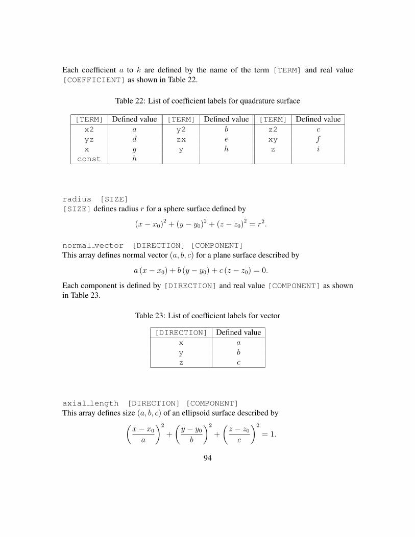
Each coefficient a to k are defined by the name of the term [TERM] and real value[COEFFICIENT] as shown in Table 22.

Table 22: List of coefficient labels for quadrature surface

[TERM] Defined value [TERM] Defined value [TERM] Defined valuex2 a y2 b z2 cyz d zx e xy fx g y h z i

const h

radius [SIZE][SIZE] defines radius r for a sphere surface defined by

(x− x0)2 + (y − y0)2 + (z − z0)2 = r2.

normal vector [DIRECTION] [COMPONENT]This array defines normal vector (a, b, c) for a plane surface described by

a (x− x0) + b (y − y0) + c (z − z0) = 0.

Each component is defined by [DIRECTION] and real value [COMPONENT] as shownin Table 23.

Table 23: List of coefficient labels for vector

[DIRECTION] Defined valuex ay bz c

axial length [DIRECTION] [COMPONENT]This array defines size (a, b, c) of an ellipsoid surface described by(

x− x0a

)2

+

(y − y0b

)2

+

(z − z0c

)2

= 1.

94

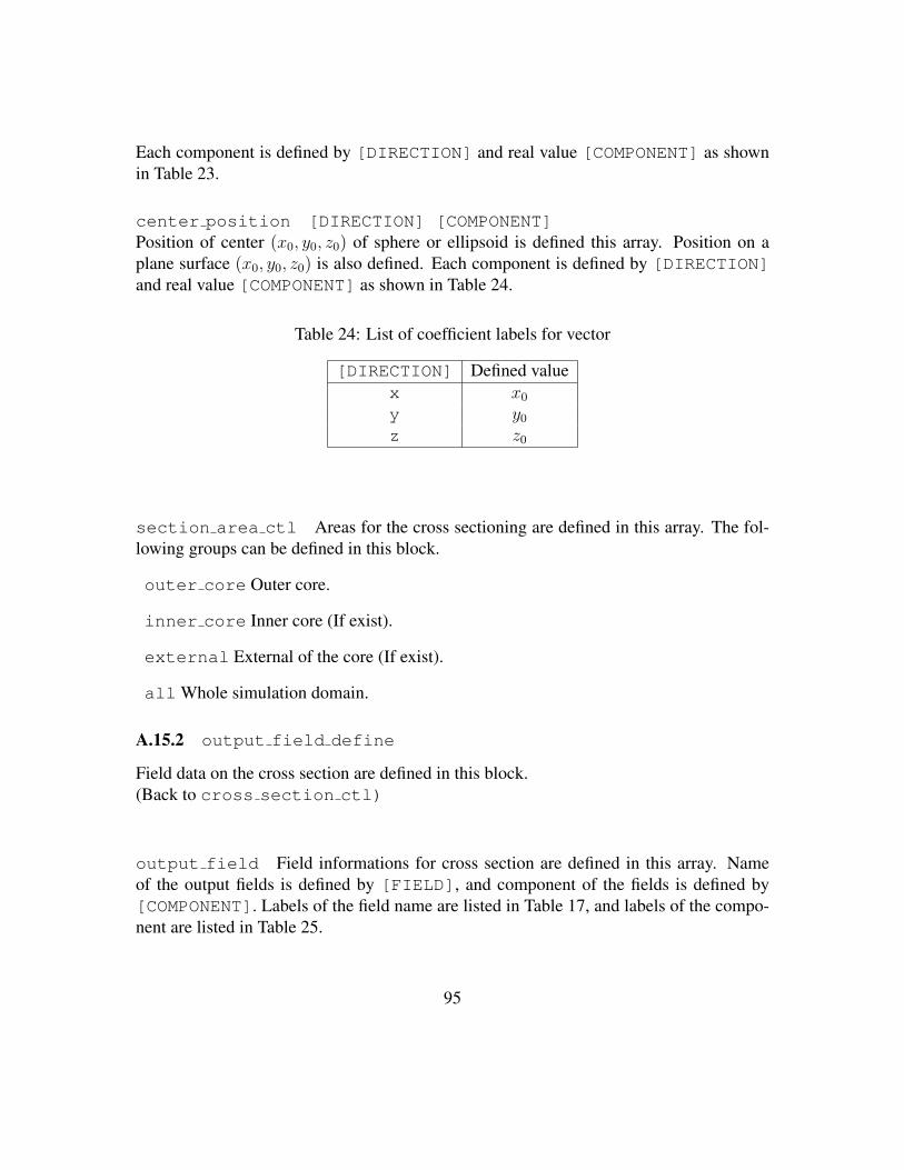
Each component is defined by [DIRECTION] and real value [COMPONENT] as shownin Table 23.

center position [DIRECTION] [COMPONENT]Position of center (x0, y0, z0) of sphere or ellipsoid is defined this array. Position on aplane surface (x0, y0, z0) is also defined. Each component is defined by [DIRECTION]and real value [COMPONENT] as shown in Table 24.

Table 24: List of coefficient labels for vector

[DIRECTION] Defined valuex x0y y0z z0

section area ctl Areas for the cross sectioning are defined in this array. The fol-lowing groups can be defined in this block.

outer core Outer core.

inner core Inner core (If exist).

external External of the core (If exist).

all Whole simulation domain.

A.15.2 output field define

Field data on the cross section are defined in this block.(Back to cross section ctl)

output field Field informations for cross section are defined in this array. Nameof the output fields is defined by [FIELD], and component of the fields is defined by[COMPONENT]. Labels of the field name are listed in Table 17, and labels of the compo-nent are listed in Table 25.

95

Table 25: List of field type for cross sectioning and isosurface module

[COMPONENT] Field typescalar scalar fieldvector Cartesian vector field

x x-componenty y-componentz z-component

radial radial (r-) componenttheta θ-componentphi φ-component

cylinder_r cylindrical radial (s-) componentmagnitude magnitude of vector

isosurface file prefix [file_prefix]File prefix for isosurface data is defined as character [file_prefix].

A.15.3 isosurf define

Each isosurface is defined in this block.(Back to isosurface ctl)

isosurf field Field name for isosurface is defined by [FIELD]. Labels of the fieldname are listed in Table 17.

isosurf component Component name for isosurface is defined by [COMPONENT].Labels of the component are listed in Table 25.

isosurf value Isosurface value is defined as real value VALUE.

isosurf area ctl Areas for the isosurfacing are defined in this array. The samegroups can be defined as section area ctl.

96

A.15.4 field on isosurf

Field data on the isosurface are defined in this block.(Back to isosurface ctl)

result type Output data type is defined by [TYPE]. Following types can be defined:

constantConstant value is set as a result field. The amplitude is set by result_value.

field field data on the isosurface are written. Fields to be written are defined byoutput_field array.

result value Isosurface value is defined as real value VALUE.

output field Field informations for cross section are defined in this array. Nameof the output fields is defined by [FIELD], and component of the fields is defined by[COMPONENT]. Labels of the field name are listed in Table 17, and labels of the compo-nent are listed in Table 25.

A.16 num domain ctl

Parallelization is defined in this block. Domain decomposition is defined for spectrumdata, field data, and Legendre transform.(Back to control sph shell)

num radial domain ctl [Ndomain]Number of subdomains in the radial direction for the spherical grid (r, θ, φ) and sphericaltransforms (r, θ,m) and (r, l,m).

num horizontal domain ctl [Ndomain]Number of subdomains in the horizontal direction. The number will be the number of sub-domains for the meridional directios for the spherical grid (r, θ, φ) and Fourier transform(r, θ,m). For Legendre transform (r, θ,m) and (r, l,m), the number will be the numberof subdomains for the h.armonics ordedr m.

97

num domain sph grid [Direction] [Ndomain]Definition of number of subdomains for physical data in spherical coordinate (r, θ, φ).Direction radial or meridional is set in [Direction], and number of subdomains[Ndomain] are defined in the integer field.

num domain legendre [Direction] [Ndomain]Definition of number of subdomains for Legendre transform between (r, θ,m) and (r, l,m).Direction radial or zonal is set in [Direction], and number of subdomains [Ndomain]are defined in the integer field.

num domain spectr [Direction] [Ndomain]Definition of number of subdomains for spectrum data in (r, l,m). Direction modes is setin the [Direction] field, and number of subdomains [Ndomain] are defined in theinteger field.

A.17 num grid sph

Spatial resolution of the spherical shell is defined in this block.(Back to control sph shell)

truncation level ctl [Lmax]Truncation level L is defined by integer. Spherical harmonics is truncated by triangular0 ≤ l ≤ L and 0 < m < l.

ngrid meridonal ctl [Ntheta]Number of grid in the meridional direction [Ntheta] is defined by integer.

ngrid zonal ctl [Nphi]Number of grid in the zonal direction [Nphi] is defined by integer.

raidal grid type ctl [explicit, Chebyshev, or equi_distance]Type of the radial grid spacing is defined by text. The following types are supported inCalypso.

explicit Equi-distance grid

Chebyshev Chebyshev collocation points

equi distance Set explicitly by r_layer array

98

num fluid grid ctl [Nr_shell](This option works with radial_grid_type_ctl is explicit or Chebyshev.)Number of layer in the fluid shell [Nr_shell] is defined by integer. Number of gridsincluding CMB and ICB will be ([Nr_shell] + 1).

fluid core size ctl [Length](This option works with radial_grid_type_ctl is explicit or Chebyshev.)Size of the outer core [Length] (= ro − ri) is defined by real.

ICB to CMB ratio ctl [R_ratio](This option works with radial_grid_type_ctl is explicit or Chebyshev.)Ratio of the inner core radius to outer core [R_ratio] (= ri/ro) is defined by real.

Min radius ctl [Rmin](This option works with radial_grid_type_ctl is explicit or Chebyshev.)Minimum radius of the domains [Rmin] is defined by real. If this value is not defined,ICB becomes inner boundary of the domain.

Max radius ctl [Rmax](This option works with radial_grid_type_ctl is explicit or Chebyshev.)Maximum radius of the domains [Rmax] is defined by real. If this value is not defined,CMB becomes outer boundary of the domain.

r layer [Layer #] [Radius](This option works with [radial_grid_type_ctl] is explicit.) List of the ra-dial grid points in the simulation domain. Index of the radial point [Layer #] is definedby integer, and radius [Radius] is defined by real.

array boundaries ctl [Boundary_name] [Layer #](This option works with [radial_grid_type_ctl] is explicit.) Boundaries of

the simulation domain is defined by [Layer #] in [r_layer] array. The followingboundary name can be defined for [Boundary_name].

to Center Inner boundary of the domain to fill the center.

ICB ICB

CMB CMB

99

A.18 new data files def

File names and number of processes for new domain decomposed data are defined in thisblock.(Back to control assemble sph)

num new domain ctl [new_num_domain]Number of subdomain for new new decomposed data [new_num_domain] is definedby integer.

new sph mode prefix [new_sph_prefix]File prefix of new spherical harmonics indexing [new_sph_prefix] is defined by text.

new restart prefix [new_rst_prefix]File prefix of new spectrum data [new_rst_prefix] is defined by text.

delete original data flag [delete_original_data_flag]If this flag set to YES, original specter data is deleted at the end of program.

A.19 newrst magne ctl

Parameters to modify magnetic field are defined in this block.(Back to control assemble sph)

magnetic field ratio ctl [ratio]Ratio of new magnetic field data to original magnetic field [ratio] is defined by real.

100

Appendix B GNU GENERAL PUBLIC LICENSECopyright c© 1989, 1991 Free Software Foundation, Inc.

51 Franklin Street, Fifth Floor, Boston, MA 02110-1301, USA

Everyone is permitted to copy and distribute verbatim copies of this license document,but changing it is not allowed.

Preamble

The licenses for most software are designed to take away your freedom to share andchange it. By contrast, the GNU General Public License is intended to guarantee yourfreedom to share and change free software—to make sure the software is free for all itsusers. This General Public License applies to most of the Free Software Foundation’ssoftware and to any other program whose authors commit to using it. (Some other FreeSoftware Foundation software is covered by the GNU Library General Public Licenseinstead.) You can apply it to your programs, too.

When we speak of free software, we are referring to freedom, not price. Our GeneralPublic Licenses are designed to make sure that you have the freedom to distribute copiesof free software (and charge for this service if you wish), that you receive source code orcan get it if you want it, that you can change the software or use pieces of it in new freeprograms; and that you know you can do these things.

To protect your rights, we need to make restrictions that forbid anyone to deny youthese rights or to ask you to surrender the rights. These restrictions translate to certainresponsibilities for you if you distribute copies of the software, or if you modify it.

For example, if you distribute copies of such a program, whether gratis or for a fee,you must give the recipients all the rights that you have. You must make sure that they,too, receive or can get the source code. And you must show them these terms so they knowtheir rights.

We protect your rights with two steps: (1) copyright the software, and (2) offer you thislicense which gives you legal permission to copy, distribute and/or modify the software.

Also, for each author’s protection and ours, we want to make certain that everyoneunderstands that there is no warranty for this free software. If the software is modified bysomeone else and passed on, we want its recipients to know that what they have is not theoriginal, so that any problems introduced by others will not reflect on the original authors’reputations.

Finally, any free program is threatened constantly by software patents. We wish toavoid the danger that redistributors of a free program will individually obtain patent li-

101

censes, in effect making the program proprietary. To prevent this, we have made it clearthat any patent must be licensed for everyone’s free use or not licensed at all.

The precise terms and conditions for copying, distribution and modification follow.

TERMS AND CONDITIONS FOR COPYING, DISTRIBUTIONAND MODIFICATION

0. This License applies to any program or other work which contains a notice placedby the copyright holder saying it may be distributed under the terms of this GeneralPublic License. The “Program”, below, refers to any such program or work, anda “work based on the Program” means either the Program or any derivative workunder copyright law: that is to say, a work containing the Program or a portionof it, either verbatim or with modifications and/or translated into another language.(Hereinafter, translation is included without limitation in the term “modification”.)Each licensee is addressed as “you”.

Activities other than copying, distribution and modification are not covered by thisLicense; they are outside its scope. The act of running the Program is not restricted,and the output from the Program is covered only if its contents constitute a workbased on the Program (independent of having been made by running the Program).Whether that is true depends on what the Program does.

1. You may copy and distribute verbatim copies of the Program’s source code as youreceive it, in any medium, provided that you conspicuously and appropriately pub-lish on each copy an appropriate copyright notice and disclaimer of warranty; keepintact all the notices that refer to this License and to the absence of any warranty;and give any other recipients of the Program a copy of this License along with theProgram.

You may charge a fee for the physical act of transferring a copy, and you may atyour option offer warranty protection in exchange for a fee.

2. You may modify your copy or copies of the Program or any portion of it, thus form-ing a work based on the Program, and copy and distribute such modifications orwork under the terms of Section 1 above, provided that you also meet all of theseconditions:

(a) You must cause the modified files to carry prominent notices stating that youchanged the files and the date of any change.

102

(b) You must cause any work that you distribute or publish, that in whole or in partcontains or is derived from the Program or any part thereof, to be licensed as awhole at no charge to all third parties under the terms of this License.

(c) If the modified program normally reads commands interactively when run, youmust cause it, when started running for such interactive use in the most ordi-nary way, to print or display an announcement including an appropriate copy-right notice and a notice that there is no warranty (or else, saying that youprovide a warranty) and that users may redistribute the program under theseconditions, and telling the user how to view a copy of this License. (Excep-tion: if the Program itself is interactive but does not normally print such anannouncement, your work based on the Program is not required to print anannouncement.)

These requirements apply to the modified work as a whole. If identifiable sectionsof that work are not derived from the Program, and can be reasonably consideredindependent and separate works in themselves, then this License, and its terms, donot apply to those sections when you distribute them as separate works. But whenyou distribute the same sections as part of a whole which is a work based on theProgram, the distribution of the whole must be on the terms of this License, whosepermissions for other licensees extend to the entire whole, and thus to each and everypart regardless of who wrote it.

Thus, it is not the intent of this section to claim rights or contest your rights towork written entirely by you; rather, the intent is to exercise the right to control thedistribution of derivative or collective works based on the Program.

In addition, mere aggregation of another work not based on the Program with theProgram (or with a work based on the Program) on a volume of a storage or distri-bution medium does not bring the other work under the scope of this License.

3. You may copy and distribute the Program (or a work based on it, under Section 2) inobject code or executable form under the terms of Sections 1 and 2 above providedthat you also do one of the following:

(a) Accompany it with the complete corresponding machine-readable source code,which must be distributed under the terms of Sections 1 and 2 above on amedium customarily used for software interchange; or,

(b) Accompany it with a written offer, valid for at least three years, to give anythird party, for a charge no more than your cost of physically performing sourcedistribution, a complete machine-readable copy of the corresponding source

103

code, to be distributed under the terms of Sections 1 and 2 above on a mediumcustomarily used for software interchange; or,

(c) Accompany it with the information you received as to the offer to distributecorresponding source code. (This alternative is allowed only for noncommer-cial distribution and only if you received the program in object code or exe-cutable form with such an offer, in accord with Subsection b above.)

The source code for a work means the preferred form of the work for making mod-ifications to it. For an executable work, complete source code means all the sourcecode for all modules it contains, plus any associated interface definition files, plusthe scripts used to control compilation and installation of the executable. However,as a special exception, the source code distributed need not include anything that isnormally distributed (in either source or binary form) with the major components(compiler, kernel, and so on) of the operating system on which the executable runs,unless that component itself accompanies the executable.

If distribution of executable or object code is made by offering access to copy froma designated place, then offering equivalent access to copy the source code from thesame place counts as distribution of the source code, even though third parties arenot compelled to copy the source along with the object code.

4. You may not copy, modify, sublicense, or distribute the Program except as expresslyprovided under this License. Any attempt otherwise to copy, modify, sublicense ordistribute the Program is void, and will automatically terminate your rights underthis License. However, parties who have received copies, or rights, from you underthis License will not have their licenses terminated so long as such parties remain infull compliance.

5. You are not required to accept this License, since you have not signed it. However,nothing else grants you permission to modify or distribute the Program or its deriva-tive works. These actions are prohibited by law if you do not accept this License.Therefore, by modifying or distributing the Program (or any work based on the Pro-gram), you indicate your acceptance of this License to do so, and all its terms andconditions for copying, distributing or modifying the Program or works based on it.

6. Each time you redistribute the Program (or any work based on the Program), the re-cipient automatically receives a license from the original licensor to copy, distributeor modify the Program subject to these terms and conditions. You may not imposeany further restrictions on the recipients’ exercise of the rights granted herein. Youare not responsible for enforcing compliance by third parties to this License.

104

7. If, as a consequence of a court judgment or allegation of patent infringement orfor any other reason (not limited to patent issues), conditions are imposed on you(whether by court order, agreement or otherwise) that contradict the conditions ofthis License, they do not excuse you from the conditions of this License. If youcannot distribute so as to satisfy simultaneously your obligations under this Licenseand any other pertinent obligations, then as a consequence you may not distributethe Program at all. For example, if a patent license would not permit royalty-freeredistribution of the Program by all those who receive copies directly or indirectlythrough you, then the only way you could satisfy both it and this License would beto refrain entirely from distribution of the Program.

If any portion of this section is held invalid or unenforceable under any particularcircumstance, the balance of the section is intended to apply and the section as awhole is intended to apply in other circumstances.

It is not the purpose of this section to induce you to infringe any patents or otherproperty right claims or to contest validity of any such claims; this section hasthe sole purpose of protecting the integrity of the free software distribution sys-tem, which is implemented by public license practices. Many people have madegenerous contributions to the wide range of software distributed through that systemin reliance on consistent application of that system; it is up to the author/donor todecide if he or she is willing to distribute software through any other system and alicensee cannot impose that choice.

This section is intended to make thoroughly clear what is believed to be a conse-quence of the rest of this License.

8. If the distribution and/or use of the Program is restricted in certain countries eitherby patents or by copyrighted interfaces, the original copyright holder who places theProgram under this License may add an explicit geographical distribution limitationexcluding those countries, so that distribution is permitted only in or among coun-tries not thus excluded. In such case, this License incorporates the limitation as ifwritten in the body of this License.

9. The Free Software Foundation may publish revised and/or new versions of the Gen-eral Public License from time to time. Such new versions will be similar in spirit tothe present version, but may differ in detail to address new problems or concerns.

Each version is given a distinguishing version number. If the Program specifies aversion number of this License which applies to it and “any later version”, you havethe option of following the terms and conditions either of that version or of any laterversion published by the Free Software Foundation. If the Program does not specify

105

a version number of this License, you may choose any version ever published by theFree Software Foundation.

10. If you wish to incorporate parts of the Program into other free programs whosedistribution conditions are different, write to the author to ask for permission. Forsoftware which is copyrighted by the Free Software Foundation, write to the FreeSoftware Foundation; we sometimes make exceptions for this. Our decision will beguided by the two goals of preserving the free status of all derivatives of our freesoftware and of promoting the sharing and reuse of software generally.

NO WARRANTY

11. BECAUSE THE PROGRAM IS LICENSED FREE OF CHARGE, THERE IS NO WAR-RANTY FOR THE PROGRAM, TO THE EXTENT PERMITTED BY APPLICABLE LAW.EXCEPT WHEN OTHERWISE STATED IN WRITING THE COPYRIGHT HOLDERS AND/OR

OTHER PARTIES PROVIDE THE PROGRAM “AS IS” WITHOUT WARRANTY OF ANY

KIND, EITHER EXPRESSED OR IMPLIED, INCLUDING, BUT NOT LIMITED TO, THE

IMPLIED WARRANTIES OF MERCHANTABILITY AND FITNESS FOR A PARTICU-LAR PURPOSE. THE ENTIRE RISK AS TO THE QUALITY AND PERFORMANCE OF

THE PROGRAM IS WITH YOU. SHOULD THE PROGRAM PROVE DEFECTIVE, YOU

ASSUME THE COST OF ALL NECESSARY SERVICING, REPAIR OR CORRECTION.

12. IN NO EVENT UNLESS REQUIRED BY APPLICABLE LAW OR AGREED TO IN WRIT-ING WILL ANY COPYRIGHT HOLDER, OR ANY OTHER PARTY WHO MAY MOD-IFY AND/OR REDISTRIBUTE THE PROGRAM AS PERMITTED ABOVE, BE LIABLE

TO YOU FOR DAMAGES, INCLUDING ANY GENERAL, SPECIAL, INCIDENTAL OR

CONSEQUENTIAL DAMAGES ARISING OUT OF THE USE OR INABILITY TO USE

THE PROGRAM (INCLUDING BUT NOT LIMITED TO LOSS OF DATA OR DATA BE-ING RENDERED INACCURATE OR LOSSES SUSTAINED BY YOU OR THIRD PARTIES

OR A FAILURE OF THE PROGRAM TO OPERATE WITH ANY OTHER PROGRAMS),EVEN IF SUCH HOLDER OR OTHER PARTY HAS BEEN ADVISED OF THE POSSIBIL-ITY OF SUCH DAMAGES.

END OF TERMS AND CONDITIONS

106

Appendix: How to Apply These Terms to Your New Pro-gramsIf you develop a new program, and you want it to be of the greatest possible use to the pub-lic, the best way to achieve this is to make it free software which everyone can redistributeand change under these terms.

To do so, attach the following notices to the program. It is safest to attach them to thestart of each source file to most effectively convey the exclusion of warranty; and each fileshould have at least the “copyright” line and a pointer to where the full notice is found.

one line to give the program’s name and a brief idea of what it does.Copyright (C) yyyy name of author

This program is free software; you can redistribute it and/or modify it underthe terms of the GNU General Public License as published by the Free Soft-ware Foundation; either version 2 of the License, or (at your option) any laterversion.

This program is distributed in the hope that it will be useful, but WITHOUTANY WARRANTY; without even the implied warranty of MERCHANTABIL-ITY or FITNESS FOR A PARTICULAR PURPOSE. See the GNU GeneralPublic License for more details.

You should have received a copy of the GNU General Public License alongwith this program; if not, write to the Free Software Foundation, Inc., 51Franklin Street, Fifth Floor, Boston, MA 02110-1301, USA.

Also add information on how to contact you by electronic and paper mail.If the program is interactive, make it output a short notice like this when it starts in an

interactive mode:

Gnomovision version 69, Copyright (C) yyyy name of authorGnomovision comes with ABSOLUTELY NO WARRANTY; for details type‘show w’.This is free software, and you are welcome to redistribute it under certainconditions; type ‘show c’ for details.

The hypothetical commands show w and show c should show the appropriate partsof the General Public License. Of course, the commands you use may be called some-thing other than show w and show c; they could even be mouse-clicks or menu items—whatever suits your program.

107

You should also get your employer (if you work as a programmer) or your school, ifany, to sign a “copyright disclaimer” for the program, if necessary. Here is a sample; alterthe names:

Yoyodyne, Inc., hereby disclaims all copyright interest in the program‘Gnomovision’ (which makes passes at compilers) written by James Hacker.

signature of Ty Coon, 1 April 1989Ty Coon, President of Vice

This General Public License does not permit incorporating your program into propri-etary programs. If your program is a subroutine library, you may consider it more usefulto permit linking proprietary applications with the library. If this is what you want to do,use the GNU Library General Public License instead of this License.

108

calypso - geodynamics · preface calypso is a program package of magnetohydrodynamics (mhd)...

Documents