CAPACITY PLANNING AND RANGE SETTING IN QUANTITY FLEXIBILITY CONTRACTS AS A MANUFACTURER

A THESIS SUBMITTED TO THE GRADUATE SCHOOL OF NATURAL AND APPLIED SCIENCES

OF THE MIDDLE EAST TECHNICAL UNIVERSITY

BY

ŞAFAK PESEN

IN PARTIAL FULFILLMENT OF THE REQUIREMENTS FOR THE DEGREE OF

MASTER OF SCIENCE

IN

THE DEPARTMENT OF INDUSTRIAL ENGINEERING

JULY 2003

Approval of the Graduate School Natural And Applied Sciences

__________________________

Prof. Dr. Tayfur Öztürk Director

I certify that this thesis satisfies all the requirements as a thesis for the degree of Master of Science.

__________________________

Prof. Dr. Çağlar Güven Head of Department

This is to certify that we have read this thesis and that in our opinion it is fully adequate, in scope and quality, as a thesis for the degree of Master of Science.

__________________________

Assoc. Prof. Dr. Sinan Kayalıgil Supervisor

Examining Committee Members

Prof. Dr. Murat Köksalan ____________________________

Assoc. Prof. Dr. Refik Güllü ____________________________

Assoc. Prof. Dr. Yasemin Serin ____________________________

Assoc. Prof. Dr. Sinan Kayalıgil ____________________________

Assist. Prof. Dr. Emre Berk ____________________________

iii

ABSTRACT

CAPACITY PLANNING AND RANGE SETTING IN QUANTITY

FLEXIBILITY CONTRACTS AS A MANUFACTURER

Pesen, Şafak

M. S., Department of Industrial Engineering

Supervisor: Assoc. Prof. Dr. Sinan Kayalıgil

June 2003, 223 pages

Quantity Flexibility contract is an arrangement where parties agree upon a scheme of

forming ranges on volumes for their future transactions. The contract is based on

setting upper and lower limits on replenishment orders as simple multiples of point

estimates updated, published and committed by the buyers. We introduce a

manufacturer with a limited capacity; also capable of subcontracting, for deliveries

with a known lead time. He offers a Quantity Flexibility (QF) contract to a buyer

while he has an active contract with another buyer serving a market with known

demand forecast distributions. Using two-stage stochastic programming we study the

effects of flexibility multiples and the environmental factors on the buyers’

incentives and manufacturer’s capacity planning. Finally, the motivations of the

Supply Chain actors to behave independently or to be involved into the integrated

iv

supply chain where information asymmetry is removed are investigated. Our

experiments underline the critical roles played by the forecast accuracy and

information sharing.

Keywords: Supply Chain Management, Supply Contracts, Quantity Flexibility,

Capacity Planning, Stochastic Programming, Benders Decomposition.

v

ÖZ

MİKTAR ESNEKLİĞİ KONTRATLARINDA İMALATÇI

AÇISINDAN KAPASİTE PLANLAMA VE ARALIK BELİRLEME

Pesen, Şafak

Yüksek Lisans, Endüstri Mühendisliği Bölümü

Tez Danışmanı: Doç. Dr. Sinan Kayalıgil

Haziran 2003, 223 sayfa

Miktar Esnekliği kontratı, tarafların gelecek siparişlerinin miktarları için aralık

belirleme metodunda anlaşma sağladığı bir düzenlemedir. Bu kontrat tipi, müşterinin

değiştirdiği, ilan ettiği ve taahhüt ettiği nokta tahminlerinin basit katları olarak alt ve

üst sınırları düzenlenen sipariş miktarlarına dayanmaktadır. Kapasitesi sınırlı, aynı

zamanda sabit tedarik zamanında fason üretimi teslim alabilen bir imalatçı ele

alınmıştır. İmalatçı, talep tahmini dağılımları bilinen bir pazara mal satan bir

müşteriyle miktar esnekliği (ME) kontratı yapmışken, başka bir müşteriye de ME

kontratı önerir. İki aşamalı rassal programlama kullanılarak esneklik çarpanlarının ve

çevresel etkilerin müşterilerin davranışlarına ve imalatçı firmanın kapasite

planlamasına etkileri incelenmiştir. Son olarak, tedarik zinciri aktörlerinin tek

başlarına hareket etme ya da tüm kararların paylaşıldığı entegre tedarik zincirine

vi

dahil olma tutumları belirlenmiştir. Deneylerimiz, tahmin doğruluğu ve bilgi

paylaşımının oynadığı kritik rolleri vurgulamaktadır.

Anahtar Kelimeler: Tedarik Zinciri Yönetimi, Tedarik Kontratları, Miktar Esnekliği,

Kapasite Planlama, Rassal Programlama, Benders Ayrışması.

vii

To my Family and Esteban

viii

ACKNOWLEDGMENTS I would like to express many thanks firstly for my dear supervisor Assoc. Prof. Dr.

Sinan Kayalıgil, not only for his endless and enduring supervision, but also for the

encouragement he provided me for research.

I also want to thank to my family for their confidence in me, and for their effort in

designing my new house, while I am writing my thesis. Thanks to my sister, Devrim,

for her motivation for research.

I owe many thanks to Filiz, for having a thesis study upon mine, and for the

excitement she gives to me to carry on everywhere and every time.

I would like to thank to Memoş for the magic opinion of Copy and Paste to Notepad,

to Pınar for Ctrl+R and Ctrl+H, to Şükran Teyze for her catering and support, to

Ozan for his technical support, and to Gülsen for her non-existing PC.

Finally, I want to express gratitude to my estimated husband, Özgür, who will be the

actual husband in 16th August, 2003, for his deep patience and love that hearten me

to study more and more to be with him as soon as possible.

ix

TABLE OF CONTENTS

ABSTRACT…………………………………………………………....

iii

ÖZ……………………………………………………………………....

v

DEDICATION………………………………………………………....

vii

ACKNOWLEDGMENTS………………………………………….......

viii

TABLE OF CONTENTS……………………………………………....

ix

LIST OF TABLES…………………………………………………......

xii

LIST OF FIGURES…………………………………………………….

xv

CHAPTER

1. INTRODUCTION…………....................................................

1

2. LITERATURE REVIEW…………………………………….

11

3. ENVIRONMENT AND MODELING……………………….

29

3.1 Environment……………………………………………

30

3.2 Modeling……………………………………………….

39

3.3 Stochastic Modeling……………………........................

49

4. TWO-STAGE STOCHASTIC MODELING AND SOLUTION METHOD............................................................

64

4.1 Two-Stage Stochastic Models and Benders Decomposition………………………………………....

65

4.2 Benders Decomposition………………………………..

77

5. EXPERIMENT…………………………………………….....

82

x

5.1 Experimental Factors…………………………………..

83

5.2 Data Generation………………………………………..

85

5.2.1 Generation of Factor Levels……………………

86

5.2.2 Generation of Demand Data……………………

101

5.3 Statistical Analysis……………………………………..

104

5.4 GAMS Model…………………………………………..

106

6. ANALYSIS………………………………………………......

108

6.1 Initial Observations………………………………….....

109

6.2 Statistical Models Constructed…………………………

120

6.3 Analysis of Test Results……………………………......

129

6.3.1 First Case: 2nd Buyer Determines her Flexibility Parameters……………………………...............

129

6.3.2 Second Case: Manufacturer Determines the Flexibility Parameters to be Offered to the 2nd Buyer…………………………………………...

140

6.3.3 Individual Cases versus Integrated Supply Chain…………………………………………...

148

7. CONCLUSION………………………………………………

158

REFERENCES………………………………………………………....

165

APPENDICES A. DEMAND DATA GENERATED FOR THE FIRST AND

SECOND BUYERS IN MEDIUM AND HIGH DEVAR…...

168

B. DEMAND DATA GENERATED FOR THE MANUFACTURER IN MEDIUM AND HIGH DEVAR…...

176

C. SAMPLES GENERATED FOR THE SUPPLY CHAIN ACTORS AND INTEGRATED SUPPLY CHAIN IN MEDIUM AND HIGH DEVAR……………………………..

184

D. GAMS MODEL OF THE TWO-STAGE STOCHASTIC MODEL OF THE FIRST BUYER…………………………... 188

xi

E. AVERAGE COST OF THE SUPPLY CHAIN ACTORS IN THE DECENTRALIZED ENVIRONMENT IN THE SECOND CASE……………………………………………..

201

F. AVERAGE COST OF THE SUPPLY CHAIN ACTORS IN THE CENTRALIZED ENVIRONMENT IN THE SECOND CASE…………………………………………………………

203

G. SINGLE FACTOR MODEL RESULTS OF THE FIRST CASE…………………………………………………………

205

H. SUBCONTRACTING OPTION USED VERSUS REALIZED REPLENISHMENT AMOUNTS THROUGH FOUR PERIODS……………………………………………..

214

I. SINGLE FACTOR MODEL RESULTS OF THE SECOND CASE………………………………………………………… 217

xii

LIST OF TABLES

TABLE

5.1 Coefficient of Variation in different DEVAR levels..................

87

5.2 Flexibility Parameters of the First Buyer in different FLEX levels............................................................................................

89

5.3 Flexibility Parameters of the Second Buyer in medium DEVAR level in the First Case.………………………………..

92

5.4 Flexibility Parameters of the Manufacturer in medium DEVAR level and in different FLEX levels in the First Case…………………………………………………………….

93

5.5 Flexibility Parameters of the Second Buyer in high DEVAR level in the First Case..................................................................

93

5.6 Flexibility Parameters of the Manufacturer in high DEVAR level and in different FLEX levels in the First Case...................

94

5.7 Total Cost versus Downward Incremental Flexibility…………

96

5.8 Total Cost versus Upward Incremental Flexibility.....................

96

5.9 Flexibility Parameters of the Manufacturer in medium DEVAR level and in different FLEX levels in the Second Case.............................................................................................

98

5.10 Flexibility Parameters of the Second Buyer in medium DEVAR level in the Second Case...............................................

98

5.11 Flexibility Parameters of the Manufacturer in high DEVAR level and in different FLEX levels in the Second Case...............

99

5.12 Flexibility Parameters of the Second Buyer in high DEVAR level in the Second Case..............................................................

99

5.13 Unit Costs of the Supply Chain Actors.......................................

100

xiii

6.1 Notations of the First Buyer’s Decisions on a Rolling Horizon.

110

6.2 Notations of the Manufacturer’s Decisions on a Rolling Horizon........................................................................................

112

6.3 Decisions of the First Buyer in her Individual Environment (Decentralized Environment)…………………………………..

114

6.4 Decisions of the Second Buyer in her Individual Environment.. 115

6.5 Decisions of the Manufacturer in his Individual Environment... 116

6.6 Decisions of the First Buyer in the Integrated Supply Chain Environment (Centralized Environment)………………………

117

6.7 Decisions of the Second Buyer in the Integrated Supply Chain Environment……………………………………………………

118

6.8 Decisions of the Manufacturer in the Integrated Supply Chain Environment……………………………………………………

119

6.9 Statistical Model Content of the First Buyer.............................

123

6.10 Statistical Model Contents of the Manufacturer.........................

124

6.11 Statistical Model Contents of the Second Buyer.........................

125

6.12 Average Costs of the Supply Chain Actors in the Decentralized Environment…………………………………….

126

6.13 Average Costs of the Supply Chain Actors in the Centralized Environment……………………………………………………

127

6.14 Cost Rankings and Comparison of Differences for SC Actors in the Decentralized Environment [First Case]………………...

130

6.15 Cost Rankings and Comparison of Differences for SC Actors in the Centralized Environment [First Case]……………….......

134

6.16 Different Results of Duncan’s Tests for the First Buyer and the Manufacturer in the Centralized Environment [First Case]……

135

6.17 Cost Rankings and Comparison of Differences for SC Actors in the Decentralized Environment [Second Case]……………...

141

6.18 Different Results of Duncan’s Tests for the Manufacturer in the Decentralized Environment [Second Case]………………...

142

xiv

6.19 Cost Rankings and Comparison of Differences for SC Actors in the Centralized Environment [Second Case]………………..

144

6.20 Different Results of Duncan’s Tests for the First Buyer and the Manufacturer in the Centralized Environment [Second Case]…

145

6.21 Decentralized versus Centralized Environments for the First Buyer in the First Case................................................................

149

6.22 Decentralized versus Centralized Environments for the First Buyer in the Second Case............................................................

150

6.23 Decentralized versus Centralized Environments for the Second Buyer in the First Case................................................................

151

6.24 Decentralized versus Centralized Environments for the Second Buyer in the Second Case............................................................

152

6.25 Decentralized versus Centralized Environments in for the Manufacturer in the First and Second Cases...............................

153

6.26 Decentralized versus Centralized Environments for the Overall System in the First Case..............................................................

155

6.27 Decentralized versus Centralized Environments for the Overall System in the Second Case..........................................................

156

xv

LIST OF FIGURES

FIGURE

3.1 Sequences of the Events……………………………………......

35

3.2 Picture of the Environment………………………………….....

37

3.3 Scheme of Product Delivery…………………………………...

38

3.4 Notation Changes on a Rolling Horizon……………………….

42

3.5 Scenario Trees of the First and Second Buyers………………...

51

3.6 Scenario Tree of the Manufacturer…………………………......

55

4.1 Benders Decomposition Algorithm………………………….....

79

5.1 The Flexibility Parameters as Decision Variables and Parameters……………………………………………………...

90

5.2 Decision Process of the Second Buyer and its Interactions……

91

5.3 Total Cost versus Downward Incremental Flexibility Graph.....

96

5.4 Total Cost versus Upward Incremental Flexibility Graph..........

97

5.5 Scenario Tree generated for the First Buyer…………………...

102

6.1 Different Cases for the Identity of the Decision Maker of the Second Buyer’s Flexibility Parameters………………………...

121

6.2 Different Environments in which the SC Actors are involved…

121

6.3 Different Levels of DEVAR, FLEX, and Cost Factors………...

122

1

CHAPTER I

INTRODUCTION

A Supply Chain (SC) is a network of organizations that are involved in the

different processes and activities that produce value in the form of products and

services in the hands of ultimate consumer. Supply Chain Management (SCM) deals

with the management of material, information and financial flows in this network

consisting of vendors, manufacturers, distributors and customers. That is, supply

chain consists of multiple decision makers with possibly conflicting objectives linked

by a flow of goods, information and funds.

Operations Management area is split into three main application contexts,

namely customer management, production management, and product development.

Customer management concerns the activities related to identify the key target

market and implement programs with key customers. Production management

includes different processes such as procurement, forecasting, order fulfillment,

quality control and planning, and logistics. Product development, when dealt with

according to SCM, involves strategies such as the design for SCM, and the design for

localization. When production management area is taken into consideration, broad

types of SCM problems in this specific context can be classified as SC configuration

and SC coordination.

2

Configuration mainly involves problems at a strategic level dealing with the

design of the supply chain network, in particular supply, production and distribution

networks. Relevant decisions in the design of the supply network concern the make

or buy problem, the supply strategy, the sourcing policies, and the manufacturer

selection process. To sum up, solving a configuration problem means to determine

the nodes of SC and related linkages as well as identify the actors that operate them.

Coordination problems concern the management of the supply chain network

prevalently under tactical and operating perspectives. Hence, the coordination

problems in a SC are quite complex that they arise from the need of integrating

operational decisions, which are generally made by several different decision

makers. Such decisions, which can concern a single function or different functions,

and involve more than one organization, should be coherently guided in order to

increase the total SC performance, that is, channel coordination. The channel

coordination is achieved in two broad categories, which are centralized and

decentralized decision making processes.

A centralized decision making process is associated with a unique decision

maker in the SC who should possess all the information on the whole SC that is

relevant with making decision as well as with the contractual power to have such

decisions to be implemented. When the decision making process is decentralized,

several decision makers exists in the SC who generally possess information on only a

part of the SC, pursue different objectives, possibly conflicting among each other.

Hence, in the selection of a SCM model appropriate to a given problem, beside the

quite obvious importance related to whether the coordination is intra functional,

3

inter-functional, or inter organizational, a key issue is to realize whether the decision

making process will occur in a centralized or decentralized fashion.

Consequently, coordination has become an important issue in the

optimization of the performance of the supply chain. Some contractual arrangements

are used to improve the efficiency of the supply chain. These arrangements include

the reallocation of decision rights, rules for sharing the costs of inventory and stock

out, and policies governing pricing either to the end customer or between supply

chain partners. In other words, a contractual arrangement, i.e. supply chain contract,

is a coordination mechanism that provides incentives to all of its members, so that

the decentralized supply chain behaves nearly or exactly the same as the integrated

one.

The contract analysis offer guidance in negotiating the terms of the

relationship between the buyer and the manufacturer, i.e., supply chain actors. Most

of the published works in the field treat the terms of contractual relationship as

decision variables, such as price, lead time, and bounds on order size.

Contracts are designed to motivate the parties to pursue certain contract

structures. Firstly, the buyer and manufacturer share the risks arising from various

sources of uncertainty. (e.g., market demand, delivery time, product quality, etc.).

Minimum purchase agreements or penalties for returns are often included in

contracts to protect the manufacturer against this risk happening. Secondly, by

channel coordination, the causes of the inefficiency of the supply chain can be

identified and the structure of the relationship can be modified. Also, by explaining

shared allowances as well as specifying penalties for non-cooperative behavior, long

term partnerships can be facilitated. Finally, like lead time, on time delivery rates and

4

conformance rates, the terms of a relationship are made explicitly in order to make

the expectations of each party concrete.

The set of parameters over which supply contracts are observed can be

classified in some categories, which are horizon length, pricing, periodicity of

ordering, quantity commitment, time and quantity flexibility, delivery commitment,

quality, and information sharing.

The main types of contracts in some of the categories declared above can be

stated as follows;

The total minimum quantity commitment: The buyer guarantees that his

cumulative orders for all periods in the contract horizon will exceed a specified

minimum quantity. In return, the manufacturer offers price discounts. Backup

agreements are in this category.

The total minimum quantity commitment with flexibility: The manufacturer

imposes restrictions on the total purchases at the discounted price. Any quantity

ordered above the restriction is available at a higher price.

The periodical stationary commitment: The buyer is required to purchase a

fixed amount in each period. Discounts are given based on the level of minimum

commitment. Additional units can be purchased at an extra cost. Often, the

manufacturer imposes restrictions on the total purchases at the discounted price. Any

quantity ordered above the restriction is available at a higher price.

The periodical commitment with order bands: The buyer is required to restrict

the order quantities to be within constant specified lower and upper limits. The unit

price depends on the band-width and increases with the band-width.

5

The periodical commitment with rolling horizon flexibility: At the beginning

of the horizon, the buyer commits to purchase given quantities every period. The

buyer has a limited flexibility to purchase quantities different from the original

commitments. The buyer is allowed to update the previously made commitments,

within a given limitation. The unit price decreases with the allowed flexibility.

Quantity flexibility contracts are included in this type of contracts.

The periodical commitment with options: At the beginning of the horizon, the

buyer commits to purchase given quantities every period. The buyer has a limited

flexibility to purchase options at unit option price from the manufacturer that allows

him to buy additional units, by paying an exercise price. So, options permit the buyer

to adjust orders quantities to the observed demands. Under some assumptions, these

contracts with options encompass backup agreements contracts, periodical

commitment contracts with flexibility (quantity flexibility contracts) and pay-to-

delay arrangements.

Delivery commitment: The manufacturer makes a commitment for the

material delivery process. A commitment on the lead time would specify delay in

delivery of the material. Thus, there a chance of adjusting lead time via the

contractual agreement. Service level agreements on lead time for the entire order or

on fraction of the order are common.

Quality commitment: The manufacturer and the buyer have a relationship

premised on the quality of the delivered product, in terms of defects rates, stipulation

of penalties for defective products. The quality is treated as a product attribute which

has a positive effect on both sales volume and production cost.

6

Information sharing: In the contractual agreement, the information flow

between a buyer and a manufacturer is characterized. The contract outlines what

types of information will be shared between the buyer and manufacturer.

Thus far, the categories described (Delft, Vial 2001) are mainly concerned

with the timing and quantity of material flows and the associated financial transfers.

The specific contracts, namely Quantity Flexibility Contracts, Backup Agreements,

Option Contract, and Pay-to-Delay Capacity Reservation Contracts will be

particularly illustrated in the following.

Quantity Flexibility contracts is a way to encourage the buyer to forecast and

plan more deliberately and honestly, on the other hand, the manufacturer might need

to provide a price break to give the buyer an incentive to participate. In such

arrangements, the buyer commits to purchase no less than a certain percentage ω

below the forecast and the manufacturer guarantees to deliver up to a certain

percentage α above the forecast. After observing the demand for a short period, the

buyer can decide to order any quantity between (1- ω)q and (1+ α)q at the wholesale

price c, where q is the initial order placed by the buyer. The QF relationship between

the manufacturer and the buyer can be described by the following parameters c, (α,

ω), where c is the transfer price.

Backup agreements are contracts between a catalog company and

manufacturers, which are similar to quantity flexibility contracts. Under a backup

agreement, the catalog company commits to purchase y units before the selling

season, and the manufacturer holds back a fraction ρ of the commitment (ρy) and

delivers the remaining units ((1-ρ)y) before the start of the fashion season. After

observing demand, the catalog company can order up to this backup quantity at the

7

same purchase price and receive quick delivery, but will pay a penalty cost b for any

backup units that it does not buy. Backup agreements intend to help catalog company

reduce the impact of uncertainty about demand.

In Option contract, before the beginning of the horizon the buyer makes three

decisions. He places firm orders for goods to be delivered at the beginning of periods

one and two at a regular price, ω. In addition, at the beginning of the selling season,

he purchases options (n) at an option price, ω0, from the manufacturer. After

observing demand in period one, he has the opportunity to order (exercise) additional

units of the product (up to the number of options purchased) at an exercise price, ωe,

before the start of period two.

Under pay-to-delay capacity reservation agreements, a buyer makes a total

reservation z of which he is obligated to purchase at least y<z units (called take-or-

pay). He pays a unit of cost cf for the take-or-pay capacity and a unit option cost of co

for z-y units. Additional units up to a maximum z-y can be bought at an extra unit of

cost of ce. That is, allocation and reservation for capacity is offered by a

manufacturer in return for a fixed up-front payment. The buyer could place orders at

a later date and use the up-front payment towards actual procurement costs. A large

portion of the allocation is usually take-or-pay capacity, for which the manufacturer

will have to pay the production cost even if he does not need the products.

Among the SCM models that adopt a decentralized decision making process,

we analyze the supply chain contracts, which include the quantity flexibility, the

backup agreements, options and pay-to-delay reservations. From these contracts,

aiming at achieving channel coordination and risk sharing among the SC actors, the

quantity flexibility contract is selected to study. Quantity flexibility models are

8

coordination mechanisms that divide the costs of demand uncertainty among the SC

actors. In this particular arrangement, the buyer, who is facing with the uncertain

demand, tries to forecast his own replenishment amounts to the manufacturer. Since

the informed amounts are only forecasts, the manufacturer, deals with, this time,

uncertain buyer’s orders. The buyer and manufacturer have their own rolling ranges,

over which quantities are restricted. Further, in the future according to the

flexibilities introduced, forecasts are given the chance of adjustment within the

specified ranges. However, these ranges are neither independent of the parties’

decisions nor are separated from one another through time. Therefore, by quantity

flexibility models, the costly effects of uncertainty on the decision making processes

of the SC actors, are tried to be reduced by giving ranges which provide the

modifications of the declared forecasts in rolling horizon basis.

A key component of decision making under uncertainty is the representation

of the stochastic parameters. Two distinct ways of representing uncertainty exist. The

scenario-based approach attempts to represent a random parameter by forecasting all

its possible future outcomes. The main drawback of this technique is that the number

of scenarios increases exponentially with the number of uncertain parameters,

leading to an exponential increase in the problem size. To avoid this difficulty,

continuous probability distributions for the random parameters are frequently used.

At the expense of introducing nonlinearities into the problem through multivariate

integration over the continuous probability space, a considerable decrease in the size

of the problem is usually achieved. This approach has been widely invoked in the

literature as it captures the essential features of demand uncertainty and is convenient

to use.

9

One of the most widely used techniques for decision making under

uncertainty is two-stage stochastic programming. In this technique, the decision

variables of the problem are partitioned in two sets. The first-stage variables, also

known as design variables, correspond to those decisions that need to be made prior

to resolution of uncertainty (“here and now” decisions). For instance, due to the

significant lead times associated with the activities such as raw material

consumption, capacity utilization, budget allocation in stock management and final

product production, decisions covering these tasks can be modeled as “here and

now” decisions. Subsequently, based on these decisions and the realization of the

random events, the second-stage or control decisions are made subject to the

restrictions of the second-stage recourse problem (“wait and see” decisions). For

example, post-production activities such as inventory management, flow of materials

throughout the production system and supply of finished good product to the

customer, can be fine-tuned in a “wait and see” setting after the realization of the

random demand. The presence of uncertainty is translated into the stochastic nature

of the costs associated with the second-stage decisions. Then, the overall objective

function consists of the sum of the first-stage decision costs and the expected second-

stage recourse costs in terms of the first stage (design) variables. Hence, the overall

problem can be expressed in two-stage stochastic programming model where there is

an interaction between the first stage (outer) and second stage (inner) problems.

Stochastic programming with recourse models are ideally suited for analyzing

resource acquisition planning problems from two perspectives. They combine

deterministic mathematical programming models for allocation resources optimally

10

with decision analysis models that provide hedging strategies in an uncertain

environment.

The main challenge associated with solving two-stage stochastic problems is

the evaluation of the expectation of the inner recourse problem. For the scenario-

based representation of uncertainty, this can be achieved by explicitly associating a

second-stage variable with each scenario and solving the large-scale formulation by

efficient solution techniques such as Dantzig-Wolfe decomposition and Benders

decomposition. For continuous probability distributions, this challenge has been

primarily resolved through discretization of the probability space for approximating

the multivariate probability integrals. The two most commonly used discretization

strategies are Monte Carlo sampling and Gaussian quadrature.

11

CHAPTER II

LITERATURE REVIEW

In Quantity Flexibility contract, the buyer is pushed to forecast and plan more

deliberately and honestly, whereas, the manufacturer might need to provide a price

break to give the buyer an incentive to participate. In this arrangement, the buyer

commits to purchase no less than a certain percentage ω below the forecast and the

manufacturer guarantees to deliver up to a certain percentage α above the forecast.

After observing the demand for a short period, the buyer can decide to order any

quantity between (1- ω)q and (1+ α)q at the wholesale price c, where q is the initial

order placed by the buyer. The QF relationship between the manufacturer and the

buyer can be described by the following parameters c, (α, ω), where c is the

transfer price.

Tsay and Lovejoy (1999) extend the QF contract in a multi-echelon SC with a

rolling production planning horizon. They study the impact of system flexibility on

inventory characteristics and the patterns by which forecast and order variability

spread along the supply chain. They also work on the design of QF contracts, i.e.

providing insights as to where to position flexibility for the greatest benefit, and how

much to pay for it, in particular by analyzing the buyer’s “willingness to pay” for

flexibility. Their analysis provides heuristics based on open loop feedback control

logic indicating how the buyer should construct his replenishment amounts in light of

12

the market demand and the flexibility parameters, as well as how the manufacturer

should behave (submission of orders, forecasting to its own upstream manufacturer)

in order to fulfill its contractual commitment to support the buyer’s order sequence.

In their extensive numerical studies, they evaluate the impact of demand variance,

flexibility parameters on the inventory costs, fill-rate, and variability in the other and

forecast processes. They conclude that the presence of flexibility can diminish the

transmission of the variability up to the chain, and suggest that inventory

management can be viewed as the management of process flexibilities. Different

from Tsay and Lovejoy, we include capacity restriction for the replenishments. We

also have the option of subcontracting in order to increase the capacity specified for

the amount to be replenished.

Tsay (1999) considers a decentralized supply relationship in which the

buyer’s advance forecast need not imply complete commitment to its subsequent

purchase quantity in response to improved demand information. Rather than

assuming a passive manufacturer who simply accommodates the buyer’s actions, he

develops a behavioral model of each party’s local incentives. By examining the

incentives on each side of the relationship, he has found that inefficiency will result

in the absence of additional structure. He identified particular forms of behavior,

such as over forecasting, or simply making decisions based on a local rather than

global perspective. He has shown that these problems can be at least partially

remedied by the QF contract, where the buyer commits to a minimum purchase and

the manufacturer guarantees a maximum coverage. He states that there is a trade off

between flexibility and unit price, with the buyer willingly paying more for increased

flexibility. He has demonstrated that incentives and information are distinct causes of

13

inefficiency. However, his results demonstrate efficiency only under shared beliefs.

The issue of coordination under information asymmetry remains unresolved.

Bassok and Anupindi (1997), analyze a supply contract for a single product

that specifies the cumulative orders placed by a buyer, over a finite horizon, be at

least as large as a given quantity. They assume the demand for the product is

uncertain and the buyer makes a commitment a priori to purchase a minimum

quantity periodically. They derive structure of the optimal purchase policy for the

buyer for a given total minimum quantity commitment and a discount price. They

show that the policy is characterized in terms of the order-up-to-levels of the finite

horizon version of the standard newsboy problem with discounted purchase price and

the order-up-to-level of a single period standard newsboy problem with no

commitment to the manufacturer but with zero purchase cost and discounted price.

Their main contributions are that they introduce the notion of a minimum

commitment over the horizon in stochastic environment and they show that this

policy can be used to evaluate and compare different contracts, determine whether a

contract is profitable, and identify the best contract. Using computational study, they

demonstrate the effect of commitments, coefficient of variation of demand,

percentage discount and penalty costs on savings.

Li and Kouvelis (1999) analyze different types of SC contracts, which are

based on quantity and time flexibility. In time inflexible contracts, the buyer is

required to specify at time 0 how many units he intends to purchase from the

manufacturer, but the contract does not require to specify when those units will be

purchased. After the buyer signed the time-flexible contract, he can observe the price

movement and decide dynamically when to trigger a buy. Besides time flexibility, in

14

SC contract with quantity flexibility, the buyer signs a contract of Q units with a

manufacturer and the contract has α x 100% quantity flexibility, where α is between

zero and one. The manufacturer does not require the buyer to purchase all Q units

from him later. The buyer can purchase a total of x units from the manufacturer

where QxQ ≤≤− )1( α . The authors develop a model where demand is deterministic

and price is uncertain. Moreover, they study the buyer’s decision when to purchase

and how many units to order in each purchase such that the expected net present

value of the purchase cost plus inventory holding cost is minimized. They discussed

optimal purchasing strategies for both time-flexible and time-inflexible contracts

with risk-sharing features and illustrate how time flexibility, quantity flexibility,

manufacturer selection, and risk sharing, when carefully exercised, can effectively

reduce the sourcing cost in environments of price uncertainty.

Bassok, Srinivasan, Bixby and Wiesel (1997) study the supply contract where

at the beginning of the contract, the buyer makes purchasing commitments to the

manufacturer for each period. The buyer may have some flexibility to purchase

quantities that actually deviate from the original commitments. Moreover, as time

passes and more information about the actual demand is collected, the buyer may

update the previous commitments, in a way that is agreed upon. They develop a

heuristic that determines nearly optimal commitments and purchasing quantities. The

heuristic is used to evaluate the worth of flexibility to adjust the commitments and

orders according to the changing conditions of the marketplace. It does capture the

dynamic nature of the problem by maximizing the probability of reaching the base-

stock levels that are optimal for the news-vendor problem and provides a mechanism

to determine the static commitments.

15

Anupindi and Bassok (1998b) address two main streams of research; analysis

and design of contracts. They focus on the issue of quantity commitments and

flexibility. They motivate and present several types of contracts structured using

quantity commitments and flexibility. The contracts; total minimum quantity

commitment, total minimum dollar volume commitment, rolling horizon flexibility

and periodical commitments with options are analyzed analytically. Their rolling

horizon flexibility contract analyzed for a multi-echelon system is called quantity

flexibility contract by Tsay and Lovejoy (1999). In RHF, at the beginning of the

horizon, the buyer commits to purchase a certain quantity every period. The buyer

has limited flexibility to purchase quantities that are somewhat different than the

original commitments, and is also allowed to update the previously made

commitments within a given range of (1-αd)Qt-1 and (1+αu)Qt-1, where αd and αu are

downward and upward flexibility parameters, respectively. They describe that the

quantity commitments provide the manufacturer with reliable information with

respect to the buyer’s overall demand and specific future orders and reduce the

uncertainty passed onto the manufacturer and share the risks due to uncertainty

between the two parties. In the paper, they concentrate on incentive contracts and

assume symmetric information between the two parties and suggest commitments

together with options as a mechanism to achieve coordination of the channel.

Bassok and Anupindi (1998) address Rolling Horizon Flexibility (RHF)

contracts. Under such a contract, a buyer has to commit orders for requirements of

components in each period, at the beginning of the horizon. Usually, the

manufacturer provides flexibility to adjust the current order and future commitments

in a limited way and in a rolling horizon fashion. They present a general model to

16

study RHF contracts and propose two measurements for the order process that

capture the variability in the order process and advance information shared between

the manufacturer and buyer through commitments. Also, they propose several

heuristics and derive a lower bound to the optimal solution of RHF contract.

Effectiveness of the heuristics for both stationary and non-stationary demands is

numerically demonstrated. Their work is similar to Tsay and Lovejoy (1999) in many

respects, but focuses on a more in-depth analysis of a single stage system which

faces non-stationary demand. They show that often “unlimited” flexibility offered by

a newsvendor model is unnecessary; larger flexibilities allow a buyer to offer higher

service levels, the variability in the order process is lower than the variability in the

demand process, the mean absolute deviation of the commitment from the actual

order decreases as we get closer to the period in which orders are placed.

Milner and Rosenblatt (1997) analyze a setting where the buyer places orders

for two periods, and may then adjust the second order after observing demand in first

period. Their study differs from the contract in Bassok and Aupindi (1997) in that

there is per unit penalty for any adjustments. They describe the optimal behavior of

the buyer, both in the initial orders and subsequent adjustment. The optimal

adjustment is characterized by a range [L, U], where the endpoints are simple

functions of the cost parameters and the demand distributions. If the pre-adjustment

inventory position on entering the second period falls in this interval, no adjustment

should be made. Otherwise, to get to the closest boundary of the interval an

adjustment is carried out. Closed forms are not available for the optimal initial

orders, but some structural properties are presented. Finally, parameter combinations,

which characterize the buyer’s preference for either the flexible contract, a non-

17

flexible contract, or no contract at all, are derived. The manufacturer’s preferences

are not considered.

Chen and Krass (2001) address a buyer-manufacturer arrangement of

particular importance namely total order quantity commitment (TOQC). They

consider the procurement and inventory control problem in which the buyer can

combine the two different purchasing strategies; purchasing on a commitment basis

and on an as-ordered basis. On the commitment basis, the buyer ensures that her

cumulative-order quantities during the contract period should be no less than the

committed amount, which she has agreed at the beginning of the contract period.

After the quantity specified in the commitment has been purchased, any additional

units can be purchased on the as-ordered basis. To encourage the buyer to commit to

greater quantities, the manufacturer usually provides a quantity discount pricing

schedule according to which, the greater the commitment, the lower the per unit

price. In addition, the buyer still reserves the flexibility to place delivery orders

depending upon her inventory replenishment policy. That is, the buyer does not have

to set a predetermined delivery schedule with the manufacturer. The optimal

inventory replenishment policy is shown to be dual order-up-to levels under a given

TOQC, and the optimal TOQC is also demonstrated to be mathematically

straightforward to obtain. They extend the model of Bassok and Anupindi (1997) to a

more general setting, which account for, non-stationary demand distributions,

different per unit prices for purchases on commitment basis and as-ordered basis.

Plambeck and Taylor (2002) consider a setting in which two buyers invest in

innovation (product development, marketing) and obtain supply from a single

manufacturer through quantity flexibility contracts, which specify the minimum

18

quantity the manufacturer must supply and the minimum quantity the buyer must

purchase. They show that the potential for renegotiation of the supply contracts has

important implications for the way firms make investments in innovation and

capacity, the way capacity is allocated, and the resulting profits of SC actors.

Conducting cooperative game theory, they provide the conditions under which the

potential for renegotiation motivates or slows down the buyer’s incentive to invest in

innovation. They demonstrate that, when the parameters of the quantity flexibility

contracts are chosen optimally, renegotiation always increases the expected total

system profit. Although renegotiation involves costly delay, managerial effort, and

legal fees, they have also assumed that renegotiation is costless.

Under a backup agreement similar to quantity flexibility contract, the catalog

company commits to purchase y units before the selling season, and the manufacturer

holds back a fraction ρ of the commitment (ρy) and delivers the remaining units ((1-

ρ)y) before the start of the fashion season. After the demand is observed, the catalog

company can order up to this backup quantity at the same purchase price and receive

quick delivery, but will pay a penalty cost b for any backup units that it does not buy.

Eppen and Iyer (1997) develop a stochastic programming model of backup

agreements. In particular, they study the impact of contract parameters (b, ρ) on the

expected catalog company’s profit. An increase in the value of b is accompanied by a

reduced advantage of using a backup agreement, whereas oppose occurs for an

increase of ρ. The latter effect is reduced by an increase of b. They also develop an

expression to measure the impact of backup agreements on the manufacturer’s profit

and show that for certain values of (b, ρ) both the catalog company and manufacturer

profits improve. They conclude that backup is an important practice in the

19

merchandising of fashion goods that can benefit both the buyer and the manufacturer,

and adjusting the order commitment in response to the offered ρ can have a

significant impact on expected profit.

In Option contract, the buyer makes a firm order, q, at the beginning of the

season at a wholesale price, ω. In addition, he purchases options (n) at an option

price, ω0. After the demand of first period is observed, the buyer may choose to order

(exercise) additional units of the product (up to the number of options purchased) at

an exercise price, ωe, before the start of period two.

Barnes-Schuster, Bassok and Anupindi (2000) investigate the role of options

in a buyer-manufacturer system. They illustrate how options provide flexibility to a

buyer to respond to market changes in the second period and demonstrate the

benefits of options in improving channel performance. They show that backup

agreements, two-period quantity flexibility contracts, and pay-to-delay arrangements

are special cases of their general model. They show that if the exercise price is

piecewise linear, channel coordination can be achieved unconditionally. The

manufacturer can then implement the channel coordination solution using either a

simple or bundled all unit quantity discount schemes. For a Stackelberg game model

of the manufacturer-buyer system in which the manufacturer is restricted to linear

pricing schemes, they numerically evaluate the value of options and coordination as a

function of demand correlation and the service level offered, providing several

managerial insights. Finally, they have illustrated how return policies, in conjunction

with linear prices, can be used to coordinate the channel and allow the manufacturer

to extract the channel profits.

20

Spinler, Huchzermeir and Kleindorfer (2002) consider contracts that provide

options as opposed to a fixed contract on the manufacturer’s capacity. Extending the

theory of real options, they propose a game-theoretic framework to value options on

capacity to produce non-storable goods or dated services, such as electricity or

transportation service. They incorporate all relevant exogenous risk factors, i.e.,

demand, price and cost risk, into a game theoretic market model for the valuation of

options on capacity. They also derive analytical expressions for the buyer’s optimal

reservation quantity and the seller’s optimal options tariff, making explicit the risk-

sharing benefits of options contracts accruing to both buyer and seller. They have

demonstrated gains in economic efficiency for the options plus spot market, which

render risk-sharing and planning instruments via options particularly attractive.

Finally, they showed that the gains increase with higher risk of finding a last-minute

buyer and with increasing cost gap between long term and short term allocation.

Under pay-to-delay capacity reservation agreements, a buyer makes a total

reservation z of which he is obligated to purchase at least y<z units (called take-or-

pay). He pays a unit of cost for the take-or-pay capacity. Additional units up to a

maximum z-y can be bought at an extra unit of cost. The buyer could place orders at

a later date and use the up-front payment towards actual procurement costs.

Brown and Lee (2000) consider a two-stage “flexible” supply contracts for

advanced reservation of capacity or advanced procurement of supply. With a contract

of this type, an initial quantity decision is made with limited demand information.

After learning new information about the demand, a final decision can be made that

is constrained by the initial decision. They consider the scenario where a large

supplier offers a standard contract to a small manufacturer. They focus on a general

21

options-futures contract that allows for initial reservation of capacity as a less

expensive, non-refundable firm commitment, i.e., futures or as a more expensive but

flexible option, i.e., options. The demand signal is defined as to be the information

that arrives after the initial decision point and before the final decision point. They

characterize the impact of demand signal quality on optimal quantity decisions. They

show that for the options-futures contract, the number of options increases and the

number of futures decreases with increasing demand signal quality. Finally, they find

that for the backup and quantity flexibility contracts, the initial order quantity does

not behave monotonically with demand signal quality. They display the bounds (1-

ω)q and (1+ α)q of QF contracts as number of futures and total reservation,

respectively.

Erkoc and Wu (2002) study capacity reservation contracts in high-tech

manufacturing, where the manufacturer shares the risk of capacity expansion with

the buyer. They focus on short-life-cycle; make to order products under stochastic

demand. The manufacturer and the buyer are defined as partners who enter a

“design-win” agreement to develop the product, and who share demand information.

The manufacturer would expand her capacity in any case, but reservation may

encourage her to expand more aggressively. To reserve capacity, the buyer pays a fee

upfront while the fee is deductible from the order payment. They show that as the

buyer’s revenue margin decreases, the manufacturer faces a sequence of three profit

scenarios for the specification of the optimal reservation fee, with a decreasing

desirability. They examine the effects of market size and demand variability to the

contract conditions, and show that it is demand variability that affects the reservation

fee. They propose two channel coordination contracts, which are capacity reservation

22

with partially deductible payments and coordination via cost sharing contracts.

Finally, they discuss additional cases where the manufacturer has the option not to

comply with the contract, and when the buyer’s market size is only partially known.

Huang, Sethi and Yan (2002) study a buyer’s problem involving a purchase

contract with a demand forecast update. Because of the presence of a lead time, the

buyer makes an initial purchase decision with a preliminary forecast. The purchase

contract provides the buyer a chance to adjust an initial commitment based on an

updated demand forecast obtained at a later stage. An adjustment, if any, incurs a

fixed as well as a variable cost. They formulate the buyer’s problem as a two-stage

dynamic programming problem, where the decisions are the initial order quantity and

the reaction plan which specifies how to adjust the initial order in view of the

improved demand information obtained at stage 2. They obtain the critical value of

the fixed contract exercise cost, below which the buyer would sign the contract.

Their model could be considered as a two-stage extension of the classical

newsvendor problem to allow for a contract, a fixed cost, a forecast update, and a

possibility of the initial order adjustment, while, at the same time, preserving the

explicitness of the solution. They prove that the optimal cost function is monotone

with respect to the contract exercise cost. In addition, they demonstrate the

asymptotic property of the cost function.

Quantity flexibility models are coordination mechanisms that divide the costs

of demand uncertainty among the SC actors. That is, QF contract involves decision

making under uncertainty. In quantity flexibility contracts, decisions are of the form;

first predict to prescribe, and then see to specify. First, the buyer predicts the demand

for the periods in the planning horizon. Then they are prescribed as forecasted

23

delivery ranges from the manufacturer. After the demand is realized, the buyer

experiences, i.e., sees the demand of the first period; he specifies the actual release

quantity for the first period to the manufacturer to be replenished. He also has the

option to adjust the estimated replenishment schedule within the specified bounds

constructed according to the QF parameters on a rolling horizon basis. Then one

period passed, and the newly predicted replenishment ranges are prescribed as

forecasted delivery ranges from the manufacturer. Consequently, the problem can be

seen as two-stage stochastic problem and can be separated in two parts. The former,

that is first stage, consists of the estimated replenishment schedule to be transferred

to the manufacturer, which is prior to realization of uncertain demand, and the latter,

that is, second stage includes the buyer’s actual replenishment schedule after the

demand appears.

Birge (1997) describes the basic methodology for the stochastic programming

models. He explores recent advances in computational capabilities for stochastic

programs and the structure of problems that enables these procedures. After

describing various solution techniques and their computational implementations, he

provides some insight into the range of possible applications of the methods through

a set of examples from actual practice such as finance, manufacturing,

telecommunication and transportation. The paper’s emphasis is on computational

methods with results in practically sized, large-scale problems. He reviewed methods

that achieve improved solutions for stochastic models over simplified deterministic

models.

Delft and Vial (2001) propose a stochastic programming approach for

quantitative analysis of supply contracts with options, involving flexibility between a

24

buyer and a manufacturer, in a supply chain framework. Specifically, they consider

the case of multi-period contracts in the face of correlated demands and briefly

reviewed the main types of the contracts in the literature. To design such contracts,

one has to estimate the savings or costs induced for parties, as well as the optimal

orders and commitments. They show how to model the stochastic process of the

demand and the decision problem for both parties using the algebraic modeling

language AMPL. They compute the optimal strategy for the buyer and manufacturer

separately. They then compare the individual performance with the global optimum

of a centralized policy in a vertical integrated framework. Finally, they compute the

economic performance of these contracts, giving evidence that the methodology

allows to gain insight into realistic problems.

Gupta and Maranas (2000) propose a two-stage stochastic programming

approach for incorporating uncertainty in multisite midterm supply chain planning

problems. In the decision making framework, the production decisions are made

“here and now” prior to the resolution of uncertainty, while the supply chain

decisions are postponed in a “wait and see” mode. The challenge associated with the

expectation evaluation of the inner optimization problem is resolved by obtaining its

closed form solution using linear programming duality. Under the normal

distribution assumption for the stochastic product demands, the evaluation of the

expected second stage costs is achieved by analytical integration resulting in an

equivalent convex mixed integer nonlinear problem. Computational requirements for

the proposed methodology are shown to be much smaller than those for Monte Carlo

sampling. In addition, the cost savings achieved by modeling uncertainty at the

planing stage are quantified on the basis of a rolling horizon simulation study.

25

Gupta, Maranas and McDonald (2000) utilize the framework of midterm,

multisite supply chain planning under demand uncertainty to safeguard inventory

reduction at the production sites and excessive shortage at the customer. A chance

constraint programming approach in conjunction with a two-stage stochastic

programming methodology is utilized for capturing the tradeoff between customer

demand satisfaction and production costs. In the proposed model, the production

decisions are made before demand realization while the supply chain decisions are

delayed until the realization of demand. The challenge associated with obtaining the

second stage recourse function is resolved by first obtaining a closed form solution of

the inner optimization problem using linear programming duality followed by

expectation evaluation by analytical integration. Furthermore, analytical expressions

for the mean and standard deviation of the inventory are derived and used for setting

the appropriate customer demand satisfaction levels in the supply chain. Finally, they

show that significant improvement in guaranteed service levels can be obtained for a

small increase in the total cost.

Chen, Li and Tirupati (2002) consider the role of product mix flexibility,

defined as the ability to produce a variety of products, in an environment

characterized by multiple products, uncertainty in product life cycles and dynamic

demands. Using a scenario-based approach for capturing the evolution of demand,

they develop a stochastic programming model for strategic decisions related to long

term technology and capacity planning. The model captures stochastic and dynamic

demand, technology mix between dedicated and flexible technologies, economies of

scope and economies of scale. Since the resulting stochastic program is quite large

and not easy to solve with standard packages, they develop a solution procedure to

26

facilitate implementation the approach. They first demonstrate their algorithm, using

augmented Lagrangian method. However, since augmented Lagrangian function is

not separable although its feasible region is separable, they propose to use restricted

simplical decomposition method which is designed to solve convex programming

problems with linear constraints more efficiently than simplical decomposition. By

the utilization of this method, they provide optimal solutions for moderate sized

nonlinear problems by solving a series of linear problems with linear costs in

reasonable time.

Liu and Sahinidis (1996) develop a two-stage stochastic programming

approach for process planning under uncertainty. The paper considers the process

planing problem with some or all of the parameters that determine the economics of

the production plan being random. They first address the case in which forecasts for

prices, demands, and availability come in a finite number of possible scenarios, each

of which has an associated probability. They take a two-stage approach to this

problem. In the first stage, they assume that, due to lead times and contractual

requirements for plant construction, capital investment decisions must be made here-

and-now. These capacity expansion decisions must be optimal in a probabilistic

sense. As the realization of the random parameters is unknown at the time of

planning, all different possible scenarios must be anticipated. Subsequently,

outcomes of the random variables will be revealed, and, for each second-stage

scenario, an optimal operating plan will be selected. Then, they devise a

decomposition algorithm for the solution of the stochastic model. The case of

continuous random variable is handled through the same algorithmic framework

without requiring any a priori discretization of their probability space. Finally a

27

method is proposed for comparing stochastic and fuzzy programming approaches

and they state that in the absence of probability distributions, the comparison favors

stochastic programming.

Schweitzer (1994) deals with two-stage and multi-stage stochastic

programming, with focusing on stochastic quadratic and convex programming, and

on stochastic programming continuous in time. In the study, the uncertainty of the

stochastic linear problems is defined by stochastic processes. An adaptation of

Benders decomposition algorithm to two-stage stochastic linear programs is

discussed and used for two-stage stochastic linear programs with large or infinite

number of scenarios. By methods of estimating expected values, an estimated

optimal value for the problem is obtained. He discusses the efficiency of that

estimator and the use of variance reduction technique to improve the estimation of

the optimal value of the problem and to reduce the number of samples that are used

by the algorithms. Two efficient algorithms to solve multi-stage stochastic linear

programs are developed. One provides an upper bound for multi-stage stochastic

linear programs with Gaussian right-hand-side. The second is an interior random

vector algorithm for multi-stage stochastic linear program.

Through flexibility contracts, the risks due to uncertainty are shared between

the manufacturer and the buyer, i.e., SC actors. The QF contract, which is one of

these flexibility contracts, is a formal agreement specifically between a manufacturer

and a buyer which explicitly specifies the buyer’s attitude for updating prior

forecasts of replenishment quantities. In most of the published works in the field,

capacity restriction of the manufacturer who guarantees to replenish the amount

within the bounds constructed with the contract parameters to the buyer, and the

28

capacity allocation risk are not taken into account, which yields a cost, in fact. This

risk happens to be due to the fact that there is an uncertain market demand with

whom the buyer is facing, and so is the manufacturer due to the buyer’s adjustable

estimated replenishment amounts.

Hence, we first intend to analyze the behavior of the manufacturer in capacity

planning while he has a limited capacity for production. Due to the obligation of

providing the prescribed release amount to the buyer, in order to relax the capacity

limitation constraint, the manufacturer is also given an outsourced production option

for analysis of his incentives.

Moreover, in literature, the contracts are usually established between a buyer

and a manufacturer, i.e., contract has two players. Thus, we are encouraged with the

challenging analysis of the case where a second buyer is introduced to the system

offering a QF contract to the manufacturer having a limited capacity for production. .

Thus far, in related works, the problem of stochastic demand in quantity

flexibility contracts is tried to be overcome by constructing the deterministic version

of the problem upon considering the worst case of the buyer’s actual release

schedule, i.e., her giving orders at the upper bound. Since the estimated

replenishment amounts are determined prior to the realization of the uncertain market

demand, and the actual ones after the realization, we aim to formulate the model of

QF contract as a two-stage stochastic programming model with the intention of

transferring the cost of uncertainty to the deterministic part of the problem as a

recourse.

29

CHAPTER III

ENVIRONMENT AND MODELING

The purpose of supply chain management (SCM) is to improve the overall

efficiency of a network of manufacturers, buyers and customers, while preserving a

decentralized approach to the decision making process. Coordination between the

supply chain (SC) actors can be achieved through appropriate exchange of

information. In this respect, contracts, one of which is Quantity Flexibility (QF)

contract, offer a large variety of possibilities to the mutual benefits of the contractors.

The environment where the SC actors exist in fact establishes the

characteristics of the interactions between the actors in a contract framework. It also

includes the type of information shared and the restrictions affecting the interactions

between the parties. We make our analysis on the basis of the incentives of the SC

actors and link their behaviors to individual and system wide performance. The

attitudes of the actors who are offered QF contract, or actors who are offering a QF

contract, are analyzed separately within the environment specified. Moreover, the

changes in the attitudes of each party are examined thoroughly, when the benefit of

the overall system is tried to be maximized. That is, we aim to present a structure for

the analysis of quantity flexibility contracts, with the particular assumptions that seek

the challenge for flexibility; suggest forecasting and ordering policies, for SC actors.

Therefore, the environment that will be pictured constitutes the core of our study.

30

The organization of this chapter is as follows. In $3.1, the description of the

environment analyzed, the definition of the problem and the underlying assumptions

are given. In $3.2, the mathematical models for supply chain contractors

individually, and for the integrated SC are illustrated. Finally, in $3.3, the stochastic

programming models for each party and the integrated supply chain constructed are

discussed.

3.1. ENVIRONMENT

We consider a supply chain composed of a single manufacturer and two

buyers. The manufacturer produces a finished good that is immediately delivered to

and sold by the buyers. The buyers sell the same product which faces a stochastic

demand. They are an intermediary between the market and the manufacturer. There

is no upstream supplier for the manufacturer. We assume that the manufacturer

produces products immediately and delivers to the buyers just after the production

and the buyers supply the market demand instantaneously. Since they face

independent market demands, they are assumed to be independent.

The first buyer has a quantity flexibility contract already agreed upon, which

is identified with the upward and downward flexibility parameters, 1ω and 1α ,

respectively. In other words, by the QF contract, the buyer commits to purchase no

less than a certain percentage 1ω below the forecast and the manufacturer guarantees

to deliver up to a certain percentage 1α above the forecast. After observing the

demand for the current period, the buyer can decide to order any quantity between

(1- 1ω )q and (1+ 1α )q, where q is the initial order placed by the buyer and ),( 11 αω

31

are the QF parameters known by the manufacturer. The buyer is allowed to carry

inventory and to backorder any unsatisfied demand for any number of periods. The

unit inventory carrying and backordering costs, are hb and bb, respectively.

As an example from the industry, Nippon Otis, a manufacturer of elevator

equipment, implicitly maintains such contract with Tsuchiya, its supplier of parts and

switches (Lovejoy 1998). Another example from the electronics industry is

Solectron, a leading contract manufacturer for many electronics firm. It has installed

such agreements with both its customer and its raw material suppliers, implying that

benefits may accrue to either end of such a contract (Ng 1997).

Upon the manufacturer’s QF contract with the first buyer, the second buyer is

introduced to the supply chain environment to study the effects of a new QF contract.

We aim to analyze the second buyer’s and the manufacturer’s incentives when the

second buyer is offered a QF contract with the manufacturer having another QF

contract already signed with the first buyer. The purpose is to explore effects of the

existing contract under limited production capacity for the manufacturer. At the

beginning of the planning horizon, the contract flexibility parameters of the second

buyer have not been specified. We try to analyze two cases where her flexibility

parameters are determined in two different ways. In the first case, the second buyer

finds out her optimal contract upward and downward flexibility parameters in the

first period, and then carries on predicting and specifying her replenishment schedule

according to the pre-found contract parameters. After the determination of the

),( 22 αω pair by herself, the contract parameters are informed to the manufacturer.

The response of the manufacturer is explained below. In the second case, the

manufacturer determines the contract flexibility parameters to be offered to the

32

second buyer. Again, at the beginning of the planning horizon, he finds out the

optimal flexibility parameters and offers to the second buyer. The second buyer is

also allowed to carry inventory and to backorder any unsatisfied demand for any

number of periods as in the first buyer’s case. She is assumed to have the same unit

inventory carrying and backordering costs as the first buyer; hb and bb ,

respectively.

The manufacturer provides the same products to the buyers who have QF

contracts associated with the contract parameters specified beforehand. The

manufacturer is given a limited capacity which is fixed so as to cover a large

percentage (we take it as 80%) of average total demands of the two buyers.

Moreover, two additional capacity options are offered to the manufacturer. The first

one is subcontracting with a constant lead time of one period. The other one is

immediate subcontracting with zero lead time for the current period in case of

inadequate limited capacity and just arrived order from the subcontractor with a

constant lead time of one period.

The manufacturer in turn, has his quantity flexibility parameters; ),( 11 mm αω

and ),( 22 mm αω particular for the first and second buyer as if he has a QF contract

with himself though he has no upstream supplier. These two flexibility pair sets are

not in relation with the flexibility parameters of the buyers. The ),( 11 mm αω pair is

stated at the beginning of the planning horizon, and the other flexibility pair,

),( 22 mm αω is the same as the one found in the two different cases which are

explained in the introduction of the second buyer. The quantity flexibility parameters

of the manufacturer can be seen as the flexibility granted to the capacity of the

manufacturer himself. From a different point of view, they can be seen as restrictions

33

generated for his release amounts. Thus, by making himself subject to the flexibility

options or subject to some restrictions for his release amounts provided by his own

QF parameters, the manufacturer is encouraged to manage his release amounts for

buyers in line with the limited capacity and additional capacity options. As said by

the QF contract, he guarantees to release the exact ordered amounts for the current

period by the two buyers, thus, he is only allowed to carry inventory. The

manufacturer has only unit costs of inventory carrying, hm , subcontracting, sm and

immediate subcontracting, subex .

It is assumed that the market demand which the buyers face is uncertain and

non-stationary and the demands for all periods are independent of each other. First,

the two buyers meet the market demand realizations for the first period and generate

the market demand forecasts for the coming periods over the finite planning horizon.

Then, according to the contract flexibility and cost parameters, they construct their

own replenishment schedules to be presented to the upstream manufacturer. These

are comprised of each one’s actual replenishment requests for the current period and

estimated replenishment amounts for the remaining periods. They also determine

their intended future replenishment amounts for the coming periods. However, these

intended future replenishment decisions are not informed to the manufacturer. They

can be seen as intended future self plans. The main function of the self plans is to

develop a course of action with tighter bounds than those asked from the

manufacturer. These have the possibility to be modified on a rolling horizon basis.

As time passed, they will be the actual replenishment amounts of the current period.

According to the actual replenishment need for the current period, and

estimated replenishment amounts for the later periods informed by the two buyers,

34

the manufacturer guarantees to release the given actual amounts for the current

period, unless they are outside the bounds denoted by QF contract. Upon taking the

given capacity limit and subcontracting options into account, he also prepares the

estimated release amounts and intended future release amounts for the coming

periods according to his own estimates for the replenishments of the buyers. He has

the same reasons (as the buyers) of being more conservative in inferring period-to-

period variation for his internal plans. Not only, the estimated release amounts, but

also the intended future release amounts can be modified on a rolling horizon basis.

If there happens to be a subcontracting decision for the second period, he

gives the order of the amount to the subcontractor due to the one period

subcontracting lead time. Unless the limited capacity and the just arrived order from

the subcontractor are insufficient; the immediate subcontracting option is never

employed. After the manufacturer supplies the exact release amounts requested by

the buyers, the buyers satisfy their realized market demand totally or partially at their

own discretion.

Then one period passes, the two buyers face the actual market demands for

the second period and they in turn modify estimated market demands for the coming

periods. Within the given bounds constructed by the contract flexibility parameters

and estimated replenishment amounts determined in the first period, the buyers

establish their new replenishment schedules. Then, they inform their schedules to the

manufacturer. On the other hand, the manufacturer faced with the new replenishment

schedules requested by the buyers reestablishes his new release schedules within his

pre-specified flexibility bounds. Upon the reestablishment, he considers his capacity

limit, and the amount ordered to the subcontractor in the first period, which has just

35

arrived, and the subcontracting options for the following periods. Then, the

manufacturer delivers the exact replenishment amounts once again, and the events

carry on in the sequence stated above for the following periods.

The sequence of the events can be seen in Figure 3.1.

Figure 3.1 Sequences of the Events

Market Demand1

realized at TMarket Demand2

realized at TInventory / Backorder1 at T-1

Replenishment Schedule1 at T-1

Intended Future Replenishments amount1 at T-1

Inventory / Backorder2 at T-1

Replenishment Schedule2 at T-1

1st Buyer prepares her Replenishment Schedule at T

2nd Buyer prepares her Replenishment Schedule at T

1st Buyer prepares her Intended Future Replenishment amounts at T

2nd Buyer prepares her Intended Future Replenishment amounts at T

Inventory1 at T-1

Release Schedule1 at T-1

Intended Future Release amounts1 at T-1

Inventory2 at T-1

Release Schedule2 at T-1

Intended Future Release amounts2 at T-1

Manufacturer prepares his Release Schedule for 1st Buyer at T

Manufacturer prepares his Release Schedule for 2nd Buyer at T

Manufacturer prepares his Intended Future Release amounts for 1st Buyer at T

Manufacturer prepares his Intended Future Release amounts for 2nd Buyer at T

Manufacturer delivers to the 1st Buyer at T

Manufacturer delivers to the 2nd Buyer at T

1st Buyer delivers to her Customers at T

2nd Buyer delivers to her Customers at T

Inventory / Backorder1 at T

Inventory / Backorder2 at T

Manufacturer’s Total Pooled Inventory at T

Inventory for 1st Buyer at T

Inventory for 2nd Buyer at T

Order is given to the Subcontractor at T

Subcontracted Order of T-1 arrives T T+1

Intended Future Replenishments amount2

at T-1

36

In accordance with the sequence of events displayed above, and the

environment illustrated in Figure 3.2, the two buyers face the realized market

demand for the current period. After the realizations of market demand, the buyers

determine their actual replenishment requests, for the current period, according to

their initial carried and backordered amounts without violating the bounds specified

by the estimated replenishment amounts settled on in the previous period. In the

current period, not only the estimated replenishment, but also the intended future

replenishment amounts for the following periods have the option to be adjusted. The

buyers try to estimate these replenishment amounts in such a way that the bounds

which will be constructed by them will neither restrict nor boost their actual

replenishment amounts in the coming periods. That is, the buyers have tradeoffs in

estimating the replenishment amounts, and in building the bounds such that they will

satisfy the realized demand without carrying too much inventory and without too

much backordering. Moreover, when low market demand is realized, by the QF

contract, they have the option of ordering less than their estimated replenishment

amounts from the manufacturer within the bounds constructed by the QF contract.

Or, when the opposite occurs, they have the opportunity to request more than their

estimated replenishment amounts without violating the bounds established.

37

Figure 3.2 Picture of the Environment

The manufacturer guarantees to release exact replenishment amounts received

from the buyer and tries to manage his limited capacity with additional

subcontracting options. Since the given estimated replenishments of the buyers have

the option to be adjusted, the manufacturer, in fact, face with uncertain actual

replenishment amounts to be asked by the buyers for the following periods.

Therefore, the manufacturer also has a tradeoff between allocating his capacity in

full, ordering large amounts to the subcontractor, hence carry inventory; versus

restricting his capacity, using the immediate subcontracting option in the current

period, which is highly expensive.

Furthermore, the same type of product is provided to both buyers. Hence, for

each buyer individually, the manufacturer has the option of pooling inventory. This

is separated from the total inventory for the satisfaction of the actual replenishment

amounts by the actual release amounts for the buyers. The potential for inventory

carrying of the manufacturer can be seen precisely in Figure 3.3.

Manufacturer

1st Buyer

2nd Buyer

Market Demand1

Market Demand2

Replenishment Order1

Replenishment Order2

Release Order1

Release Order2

Replenishment Order1

Replenishment Order2

Market Demand1

Market Demand2

Release Schedule1

Release Schedule2

Replenishment Schedule1

Replenishment Schedule2

Product Flow Information Flow

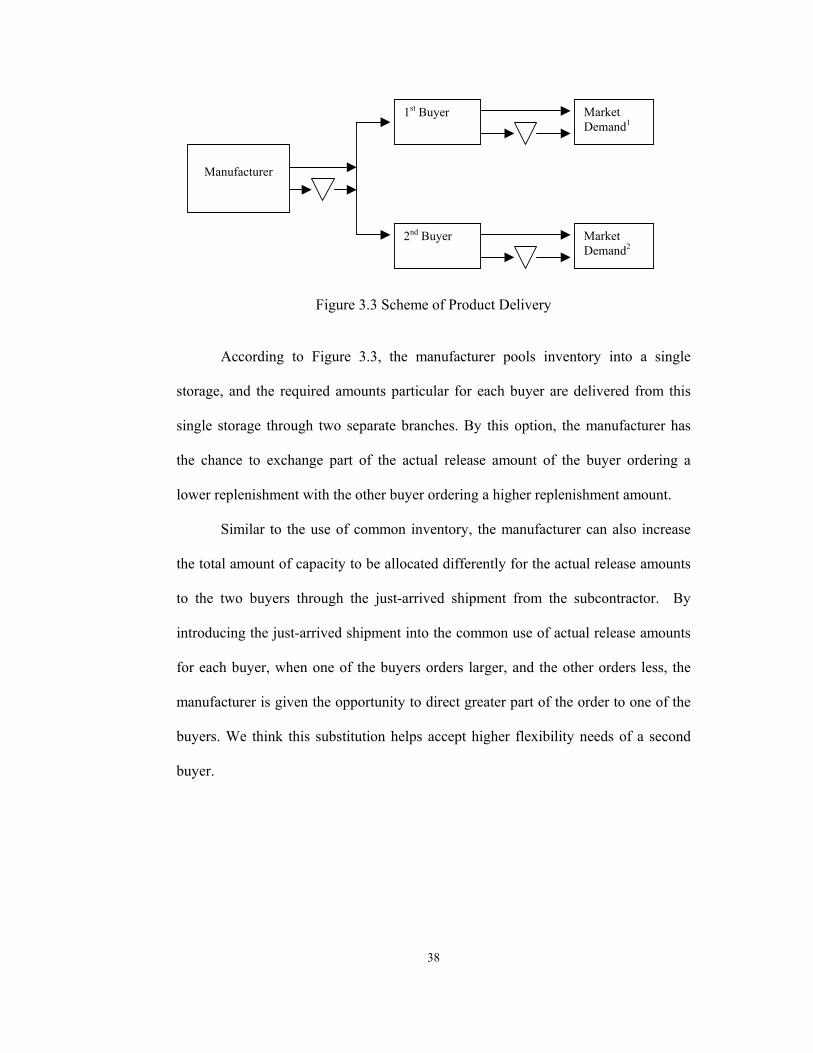
38

Figure 3.3 Scheme of Product Delivery

According to Figure 3.3, the manufacturer pools inventory into a single

storage, and the required amounts particular for each buyer are delivered from this

single storage through two separate branches. By this option, the manufacturer has

the chance to exchange part of the actual release amount of the buyer ordering a

lower replenishment with the other buyer ordering a higher replenishment amount.

Similar to the use of common inventory, the manufacturer can also increase

the total amount of capacity to be allocated differently for the actual release amounts

to the two buyers through the just-arrived shipment from the subcontractor. By

introducing the just-arrived shipment into the common use of actual release amounts

for each buyer, when one of the buyers orders larger, and the other orders less, the

manufacturer is given the opportunity to direct greater part of the order to one of the

buyers. We think this substitution helps accept higher flexibility needs of a second

buyer.

Manufacturer

1st Buyer

2nd Buyer

Market Demand1

Market Demand2

39

3.2. MODELING

To evaluate the impact of a given contract on the behavior of the SC actors

and on the performance of the system, it is necessary to perform a quantitative

analysis. Analytically, this necessitates building a mathematical model that describes

the environment (demand, capacity and subcontracting decisions, and sequence of

the events stated in the previous section.) and the use of mathematical tools to treat

these models. To illustrate our point, we focus on the model for quantity flexibility

contract presented by Tsay and Lovejoy (1999). Different from Tsay and Lovejoy,

we add the second buyer into the supply chain environment. We intend to analyze

not only the second buyer’s incentives when she is offered a QF contract with a

manufacturer, but also the manufacturer’s incentives when he has a QF contract with

a buyer and offers a QF contract to another buyer. Furthermore, a capacity limitation

for the release amounts of the manufacturer is introduced. Also, two subcontracting

options with constant lead times of one period and zero period, are included in the

capacity consideration. That is, the manufacturer is given costly capacity options to

be able to guarantee the replenishment schedules formed by the buyers.

In this study, we try to address the objectives; (i) to provide a structure for the

analysis of quantity flexibility contracts, with the assumption of non-stationary and

uncertain market demand that offer a challenge for flexibility; (ii) suggest forecasting

and ordering policies, for buyers who are obliged to purchase a certain fraction of

their estimates, for manufacturer who guarantees to provide a certain amount of the

buyer’s replenishment amounts; (iii) link all these behaviors to individual and system

wide performance, and (iv) see the impact of parameters on the behaviors.

40

Our supply chain planning problem involves medium and short term decision

types. The former, includes outsourced production capacity and range setting

decisions, and the latter comprises of decisions on production, inventory holding, and

allocation of flexible capacity. Medium term typically refers to months, whereas

short term is in the order of days or weeks.

In order to carry out quantitative analysis for the described multi period

supply chain problem, we construct models to be presented immediately after the

related notations are displayed.

BUYERS’ CASE:

The notations used for the first and second buyers are as in the following;

T :number of periods in the finite planning horizon.

)(0 tbM :realized demand of buyer b in the current period t, where b=1, 2.

)(0 jtbM + :random demand occurrence of buyer b in period (t+j), where b=1, 2, and

j=1,…,T-1.

)(0 jtbf + :actual replenishment amount of buyer b in period (t+j), which is intended

future replenishment amount, for all periods except current period t. b=1, 2 and

j=0,…,T-1.

)(tbf j :estimated replenishment amount of period (t+j) of buyer b, which is passed

on to the manufacturer in period t. b=1, 2, and j=1,…, T-1.

)( jtinvb + :amount of ending inventory of buyer b in period (t+j), where b=1, 2 and

j=0,…, T-1.

)( jtbackb + :amount of backordered demand by buyer b in period (t+j), where b=1,

2 and j=0,…,T-1.

41

),( bb αω :downward and upward flexibilities for buyer b, where b=1,2.

],...,,,[ 1321bT

bbbb−= ωωωωω , ],...,,,[ 1321

bT

bbbb−= ααααα

),( bb ΑΩ :cumulative downward and upward flexibilities for buyer b, where b=1,2.

],...,,,[ 1210bT

bbbb−ΩΩΩ=Ω ω , ],...,,,[ 1210

bT

bbbb−ΑΑΑΑ=Α

hb :unit inventory holding cost for both buyers per period.

bb :unit backordering cost for both buyers per period.

There is a relation between ),( bb αω and ),( bb ΑΩ , which can be expressed

as in the following equations;

∏=

−=Ω−j

q

bq

bj

1

)1(]1[ ω and ∏=

+=Α+j

q

bq

bj

1

)1(]1[ α

The number of periods in the finite planning horizon does not differ as time

passes. That is, the horizon length does not decrease. Thus, the current period is

always represented with the same index t, and the later periods with the index (t+j),

as time passes. It is illustrated more precisely in Figure 3.4. Also, from the figure, the

relation between the actual replenishment amounts, )(0 jtbf + and the estimated

replenishment amounts, )(tbf j can be captured.

42

Figure 3.4 Notation Changes on a Rolling Horizon

Buyers’ Model (BUY-DETb):

The model for the buyer b can be stated briefly as in the following;

Min ∑−

=

+×++×1

0)]()([

T

jjtbackbbbjtinvbhb

s.t.

)()()1()1()()( 00 jtbMjtbfjtbackbjtinvbjtbackbjtinvb +−++−+−−+=+−+

1,,0 −=∀ Tj Κ (1)

)1()1()()1()1( 1111 −+≤≤−− ++++ tbftbftbf jbjjj

bj αω 2,,0 −=∀ Tj Κ (2)

)()1()()()1( 0 tbfjtbftbf jbjj

bj Α+≤+≤Ω− 1,,0 −=∀ Tj Κ (3)

The objective function of the buyer’s model is the minimization of inventory

and backordering costs.

t+T-1t t+1 t+2 t+3

f0b(t)

f0b(t+1) f0b(t+2) f0b(t+3) f0b(t+T-1)

f1b(t) f2b(t) f3b(t) fT-1b(t)

t+T-1t t+1 t+2 t+3

t+T-1 t t+1 t+2 t+3

Buyer’s Horizon

Buyer’s Horizon

Buyer’s Horizon

One Period passes

One Period passes

f0b(t)

f0b(t+1) f0b(t+2) f0b(t+3) f0b(t+T-1)

f1b(t) f2b(t) f3b(t) fT-1b(t)

f0b(t)

f0b(t+1) f0b(t+2) f0b(t+3) f0b(t+T-1)

f1b(t) f2b(t) f3b(t) fT-1b(t)

43

(1) Inventory Balance constraints, imply the market demand in period t,

)(0 jtbM + can be satisfied totally or partially by the actual replenishment amount in

period (t+j), )(0 jtbf + .

(2) Incremental Revision constraints, imply the estimated replenishment

amount for future period (t+j), )(tbf j , can not be revised upward by a fraction of

more than αj+1b or downward by more than ωj+1

b of the estimated replenishment

amounts determined in the previous period (t+j-1), )1(1 −+ tf j .

(3) Cumulative Flexibility constraints, imply the estimated replenishment

amount for period (t+j) determined in the current period t, )(tbf j , suggests bounds

on the decision for the actual replenishment amount for period (t+j), )(0 jtbf + .

In other words, the replenishment amounts for the second and later periods

(t+j) where j=1,…,T-1, are estimated in the current period t. These estimated

replenishment amounts, )(tbf j ’s, establish bounds for the intended future

replenishment amounts for period (t+j), )(0 jtbf + . The incremental revision

constraints puts bounds on estimated replenishment amounts based on earlier

estimates and the cumulative constraints puts bounds on actual replenishment

amounts based on the estimated replenishment amounts.

MANUFACTURER’S CASE:

For the manufacturer, the following notations are used;

T :number of periods in the finite planning horizon.

)(0 tbf :realized actual replenishment amount of buyer b in the current period

t, where b=1, 2.

44

)(0 jtbf + :random occurrence of actual replenishment of buyer b in period (t+j),

where b=1, 2 and j=1,…T-1.

)(0 jtbr + :actual release amount for the request of buyer b in period (t+j), which is

intended future release amount except r0b(current period t). b=1, 2 and j=0,…,T-1.

)(tbrj :estimated release amount of period (t+j) for buyer b in period t, where b=1, 2,

and j=1,..., T-1.

)( jtinvmb + :amount of ending inventory for buyer b in period (t+j), where b=1, 2

and j=0,…, T-1.

)( jtinvmpb + :amount of inventory taken from the total pooled inventory for buyer

b in period (t+j), for the usage in period (t+1), where b=1, 2 and j=0,…,T-1.

)(tSUB :order arrived in period t, which is given to the subcontractor in period (t-1).

)( jtsub + :amount of order given to the subcontractor in period (t+j-1) and to have

delivered in period (t+j), where j=0,…,T-1.

bsub exp :amount of order given to the subcontractor in the current period t, and to

be delivered in that period, where b=1,2.

)( jtcap + :amount of capacity used for the sum of the actual release amounts in

period (t+j), where j=0,…,T.

CAP :fixed capacity available through all periods.

),( mbmb αω :downward and upward flexibilities for the manufacturer particular for

buyer b, where b=1, 2.

],...,,,[ 1321mbT

mbmbmbmb−= ωωωωω , ],...,,,[ 1321

mbT

mbmbmbmb−= ααααα

),( bb ΑΩ :cumulative downward and upward flexibilities for the manufacturer for

particular buyer b, where b=1,2.

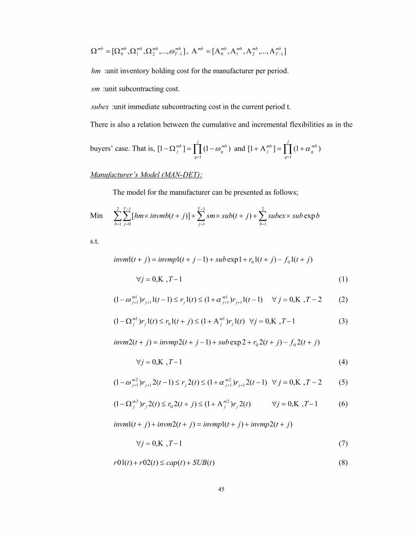
45

],...,,,[ 1210mbT

mbmbmbmb−ΩΩΩ=Ω ω , ],...,,,[ 1210

mbT

mbmbmbmb−ΑΑΑΑ=Α

hm :unit inventory holding cost for the manufacturer per period.

sm :unit subcontracting cost.

subex :unit immediate subcontracting cost in the current period t.

There is also a relation between the cumulative and incremental flexibilities as in the

buyers’ case. That is, ∏=

−=Ω−j

q

mbq

mbj

1

)1(]1[ ω and ∏=

+=Α+j

q

mbq

mbj

1

)1(]1[ α

Manufacturer’s Model (MAN-DET):

The model for the manufacturer can be presented as follows;

Min ∑∑ ∑∑=

−

= =

−

=

×++×++×2

1

1

0

2

1

1

1

exp)()]([b

T

j b

T

j

bsubsubexjtsubsmjtinvmbhm

s.t.

)(1)(11exp)1(1)(1 00 jtfjtrsubjtinvmpjtinvm +−+++−+=+

1,,0 −=∀ Tj Κ (1)

)1(1)1()(1)1(1)1( 1111

11 −+≤≤−− ++++ trtrtr j

mjjj

mj αω 2,,0 −=∀ Tj Κ (2)

)(1)1()(1)(1)1( 10

1 trjtrtr jmjj

mj Α+≤+≤Ω− 1,,0 −=∀ Tj Κ (3)

)(2)(22exp)1(2)(2 00 jtfjtrsubjtinvmpjtinvm +−+++−+=+

1,,0 −=∀ Tj Κ (4)

)1(2)1()(2)1(2)1( 1211

21 −+≤≤−− ++++ trtrtr j

mjjj

mj αω 2,,0 −=∀ Tj Κ (5)

)(2)1()(2)(2)1( 20

2 trjtrtr jmjj

mj Α+≤+≤Ω− 1,,0 −=∀ Tj Κ (6)

)(2)(1)(2)(1 jtinvmpjtinvmpjtinvmjtinvm +++=+++

1,,0 −=∀ Tj Κ (7)

)()()(02)(01 tSUBtcaptrtr +≤+ (8)

46

)()()(02)(01 jtsubjtcapjtrjtr +++≤+++ 1,,1 −=∀ Tj Κ (9)

CAPjtcap ≤+ )( 1,,0 −=∀ Tj Κ (10)

The objective function of the manufacturer’s model is the minimization of

inventory carrying, subcontracting and immediate subcontracting costs.

(1) and (4), Inventory Balance constraints, imply the actual replenishment

amount of buyer b in period (t+j), )(0 jtbf + should be satisfied exactly, by the

actual release amount in period (t+j), )(0 jtbr + .

(2) and (5), Incremental Revision constraints, imply the estimated release

amount for future period (t+j), )(tbrj , can not be revised upward by a fraction of

more than αj+1m or downward by more than ωj+1

m of the estimated release amount

determined in the previous period (t+j-1), )1(1 −+ tbrj .

(3) and (6), Cumulative Flexibility constraints, imply the estimated release

amount for period (t+j) determined in the current period t, )(tbrj , suggests bounds on

the decision for the actual release amount for period (t+j), )(0 jtbr + .

(7) Inventory Pooling constraints, imply inventory carrying decisions

resulting from the satisfaction of the actual replenishment amounts are served by the

total pooled inventory from which the required amounts can be released separately.

(8), (9), and (10) Capacity Limitation constraint, imply the sum of the actual

release amounts in period (t+j) for both buyers can not exceed the capacity limit. We

have a costly option to each of the given constant capacity limit for later periods.

Due to one period lead time subcontracting, the order given in the period t won’t be

on hand until period (t+1).

47

Quantity Flexibility contracts, help improve the joint performance of the

buyers and the manufacturer acting independently within the contract framework. To

this end, buyers face random market demand. The buyers only know the actual

market demand for the current period and they forecast for the coming periods. After

the realization of market demand of the current period, they convey information on

the actual replenishment and estimated replenishment amounts that they will request,

to the manufacturer. On the other hand, the manufacturer has his own ordering

information for the buyers, where only the actual replenishment amounts for the

current period is identified exactly as soon as he is informed and later periods’ actual

replenishment amounts are random. In other words, the manufacturer has no

information about the market demand. The manufacturer only knows the exact actual

replenishment amounts for the current period, and forecasts the replenishment

amounts for the coming periods for his future plans. Hence, there is information

discrepancy between the SC parties, where the buyers face market demand, and the

manufacturer faces replenishment amounts.

INTEGRATED SUPPLY CHAIN ENVIRONMENT:

Under the consideration of random market demand assumption, we construct

an integrated supply chain model, where the buyers’ actual replenishment amounts

for the current period and intended future replenishment amounts for the following

periods, are directly and immediately transmitted to the manufacturer as their exact

amounts. However, in the separate case, the buyers did not inform their intended

future replenishment amounts to the manufacturer. That is to say, in the integrated

SC model, there is no information asymmetry between the supply chain actors. All

48

information about the market demand, intended future replenishment decisions of the

buyers are passed on to the manufacturer, so are the information of intended future

release and subcontracting decisions of the manufacturer to the buyers.

All assumptions and particular parameters stated before the separate

formulations of the models of SC actors are also valid for the integrated supply chain

model.

Then, the model constructed for the integrated supply chain can be presented

as follows;

Integrated Supply Chain Model (INTSC-DET):

Min ∑∑=

−

=

++×++×2

1

1

0

)]()([b

T

j

jtbackbbbjtinvbhb

∑∑ ∑∑=

−

= =

−

=

×++×++×2

1

1

0

2

1

1

1

exp)()]([b

T

j b

T

j

bsubsubexjtsubsmjtinvmbhm

s.t.

Equations (1), (2), and (3) in the formulations of BUY-DET1 and BUY-DET2.

Equations (2), (3), (5), (6), (7), (8), (9), and (10) in the formulation of MAN-DET.

)(1)(11exp)1(1)(1 00 jtfjtrsubjtinvmpjtinvm +−+++−+=+ 1,,0 −=∀ Tj Κ (1)

)(2)(22exp)1(2)(2 00 jtfjtrsubjtinvmpjtinvm +−+++−+=+

1,,0 −=∀ Tj Κ (2)

The objective function of the integrated SC model is the minimization of

aggregated inventory carrying and backordering costs of the buyers; inventory

carrying, subcontracting and immediate subcontracting costs of the manufacturer.

49

(1) and (2), Inventory Balance constraints of the manufacturer for each buyer,

imply that the actual replenishment amount of buyer b in period (t+j), )(0 jtbf + ,

should be satisfied totally, by the actual release amount in period (t+j), )(0 jtbr + . In

these constraints, )(0 tperiodcurrentbf is the actual replenishment amount of buyer

b, and )(0 jtbf + is the intended future replenishment amount for period (t+j)

determined by buyer b, that is, )(0 jtbf + ’s are not random.

In the buyer’s case, )(10 jtM + and )(20 jtM + ’s in inventory balance

constraints are the random demand occurrences for the first and second buyers,

respectively. For the manufacturer’s case, )(0 jtbf + ’s in inventory balance

constraints are the random actual replenishment amounts of each buyer. In this

integrated supply chain model, since )(0 jtbf + ’s become a common decision for

both parties, only )(0 jtbM + ’s of each buyer are random demand occurrences for the

buyers, and the manufacturer faces the determined actual replenishment amounts.

3.3. STOCHASTIC MODELLING

In view of the fact that the market demand is not deterministic, the problem

under consideration happens to be a stochastic linear program. For the involvement

of the stochastic demand into the problem, a scenario based approach is utilized. A

scenario can be defined as a combination of the realizations of the stochastic

variables, i.e., market demand for all periods in the planning horizon.

In our study, the stochastic variables for the first and second buyers are the

uncertain market demand. Since, these variables occur in inventory balance

50

constraints, the actual replenishment decision variables are constructed scenario

based, so are the inventory carrying and backordering decision variables.

However, for the manufacturer, the actual replenishment amounts are the

stochastic variables. Thus, the actual release decision variables in inventory balance

constraints are constructed scenario based. Since the actual release decision variables

are involved also in the capacity limitation constraints where the subcontracting

decision variables are stated, these variables are also scenario based. The

subcontracting decisions for each period are constructed according to the

combination of pairs of scenarios of the actual replenishment amounts of the buyers.

For the manufacturer, there will be a unique set of decisions which consists of the

amounts of inventory carried, inventory pooled, actual release amounts for the first

and second buyer, and amount of order to be given to the subcontractor, for each

period in a given scenario.

We introduce the assumption that the random market demands are described

by finitely many mutually exclusive scenarios each with its particular probability.

That is, the random market demand, Mt+1, Mt+2,…Mt+T-1, is assumed to have a

discrete probability distribution. Mt,sc is demand with probability psc, where sc

denotes the particular scenario. Scenarios can be represented by scenario trees, where

each branch correspond to a scenario, sc. This makes it possible to formulate the

deterministic equivalent of the problem as a finite dimensional mathematical

programming problem, where deterministic variables are continuous and the random

variables are discrete. Many of the studies in the field employ discrete probability

distribution assumption in order to solve the stochastic programming models. In case

random variables are continuous; the formulation will result in nonlinearities.

51

Furthermore, in the scenario based decision problem we are formulating, we

have to include nonanticipativity constraints, implying that we can not anticipate the

future. A solution to a stochastic programming problem, in the form of a sequence of

responses to random events, is nonanticipative if each given response depends only

on the past events and not on future events. That is, the future is uncertain and so

today’s decision can not take the advantage of knowledge of the future. For instance,

when the levels of a scenario tree are taken into consideration, scenarios with a

common history, i.e., who inherit from the same branch of the tree, must (logically)

have the same set of decisions as the common ancestors.

BUYERS’ CASE:

According to the scenario based approach with discrete random variables, we

have generated a scenario tree with 4 levels for the buyers. This represents 4 time

periods in the planning horizon for the buyers. On the first level, there is only one

demand value with probability one, since the market demand of the current period is

a realized amount of a random demand process. The same holds true for the second

buyer. The scenario tree, which is the same in principle for both buyers, is presented

in Figure 3.5.

Figure 3.5 Scenario Tree of the First and Second Buyers

REALIZED DEMAND

A B

E F

K L M N K L M N K L M N K L M N N

G H

C D

H

52

In the figure above, following the current period, i.e., the top of the tree, in

the second and later periods, there are 4 possible demand occurrences.

From the tree in the figure, the nonanticipativity occurrences can be easily

captured. For instance, every one of the 64 scenarios inherits from a single node

resulting in the same carried inventory or backordered amount of the first period. For

instance, the first 16 scenarios, at the bottom of the scenario tree, stem from a single

branch on the second level, implying that they have the same value for the ending

inventory or backordered amounts in the second period. Thus, scenarios, which stem

from the same branch, i.e., which share a common history, have the same set of

inventory carrying and backordering decisions to inherit from.

For the stochastic programming models, the notations are somewhat

modified. The notations used for the buyers are the following;

T :number of periods in the finite planning horizon.

SC :number of scenarios generated.

klbsc , :scenarios at level l with common ancestor k, where l=1,…,T-1.

),(0 bsctbM :actual market demand of buyer b in the current period t under scenario

scb, where b=1,2 and scb=1,…SC. It has identical values for all scenarios, 1 through

SC.

),(0 bscjtbM + :random demand occurrence of buyer b in period (t+j) under

scenario scb , where b=1, 2, j=0,…,T-1 and scb=1,…,SC.

),(0 bscjtbf + :actual replenishment amount of buyer b in period (t+j) under

scenario scb, which is intended future replenishment for all periods except current

period t. b=1, 2, j=0,…,T-1 and scb=1,…,SC.

53

)(tbf j :estimated replenishment amount of period (t+j) of buyer b in period t, which

is passed onto the manufacturer. b=1, 2 and j=0,…,T-1. It is assumed that )(tbf j ’s

are statistically independent of ),(0 bscjtbf + ’s.

),( bscjtinvb + :amount of ending inventory of buyer b in period (t+j) under scenario

scb, where b=1, 2, j=0,…,T-1 and scb=1,…,SC.

),( bscjtbackb + :amount of backordered demand by buyer b in period (t+j) under

scenario scb, where b=1, 2, j=0,…,T-1 and scb=1,…,SC.

)( bscprobb :probability associated with scenario scb for buyer b, where b=1,2 and

scb=1,…,SC.

The ),( bb αω and ),( bb ΑΩ pair, hb and bb notations are same as in BUY-DET1 and

BUY-DET2.

Buyers’ Stochastic Model (BUY-STOCHb):

Then, the stochastic programming model for the buyers can be stated briefly

as in the following;

Min ]),(),()[(1

1

0∑∑

=

−

=

+×++×SC

sc

T

jbbb

b

scjtbackbbbscjtinvbhbscprobb

s.t.

),(),(),1(),1(),(),(

00 bbbb

bb

scjtbMscjtbfscjtbackbscjtinvbscjtbackbscjtinvb

+−++−+−−+=+−+

SCscandTj b ,,11,,0 ΚΚ =∀−=∀ (1)

)1()1()()1()1( 1111 −+≤≤−− ++++ tbftbftbf jbjjj

bj αω 2,,0 −=∀ Tj Κ (2)

)()1(),()()1( 0 tbfscjtbftbf jbjbj

bj Α+≤+≤Ω−

54

SCscandTj b ,,11,,0 ΚΚ =∀−=∀ (3)

),(),( ,, klb

klb csjtinvbscjtinvb ′+=+

SCscandTj klb ,,11,,0 , ΚΚ =∀−=∀ (4)

The objective function of the buyer’s model is the minimization of the

expected inventory carrying and expected backordering costs.

(1) Inventory Balance constraints, imply the market demand in period (t+j)

under scenario scb, ),(0 bscjtbM + can be satisfied totally or partially, by the actual

replenishment amount in period (t+j) under scenario scb, ),(0 bscjtbf + .

(2) Incremental Revision constraints, imply estimated replenishment amount

for future period (t+j), )(tbf j can not be revised upward by a fraction of more than

αj+1b or downward by more than ωj+1

b of the estimated replenishment amounts

determined in the previous period, (t+j-1), )1(1 −+ tbf j .

(3) Cumulative Flexibility constraints, imply the estimated replenishment

amount for period (t+j) determined in the current period t, )(tbf j , suggests bounds on

the decision for the actual replenishment amount for period (t+j) under scenario scb,

),(0 bscjtbf + .

(4) Nonanticipativity constraints, imply the scenarios having a common

history have the same set of inventory carrying and backordering decisions to inherit

from. That is, they aren’t identical for all periods but start with identical figures so

much as the common ancestors.

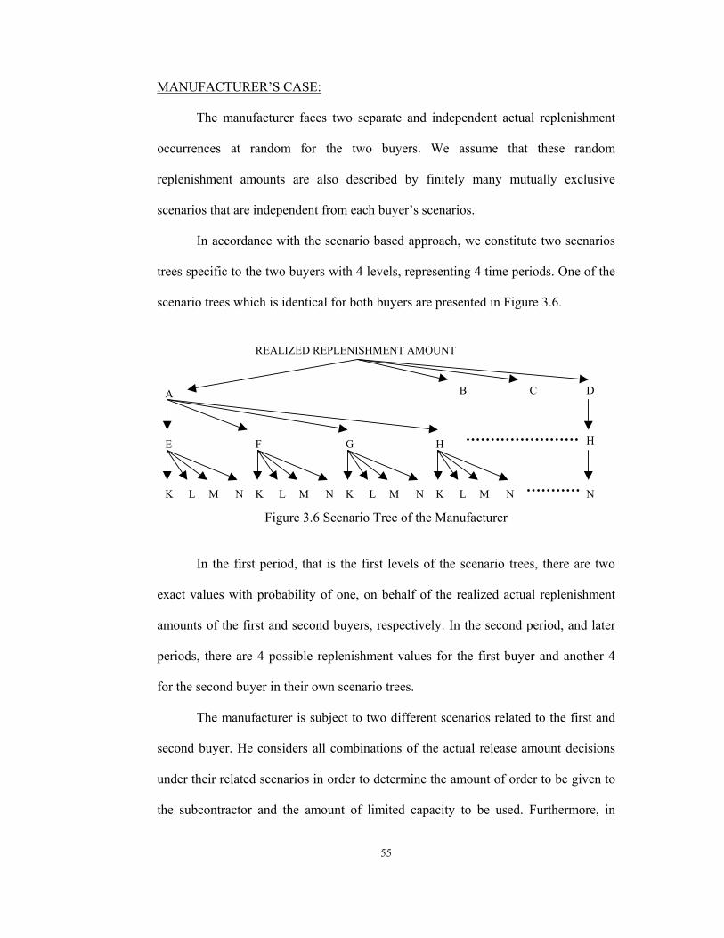
55

MANUFACTURER’S CASE:

The manufacturer faces two separate and independent actual replenishment

occurrences at random for the two buyers. We assume that these random

replenishment amounts are also described by finitely many mutually exclusive

scenarios that are independent from each buyer’s scenarios.

In accordance with the scenario based approach, we constitute two scenarios

trees specific to the two buyers with 4 levels, representing 4 time periods. One of the

scenario trees which is identical for both buyers are presented in Figure 3.6.

Figure 3.6 Scenario Tree of the Manufacturer

In the first period, that is the first levels of the scenario trees, there are two

exact values with probability of one, on behalf of the realized actual replenishment

amounts of the first and second buyers, respectively. In the second period, and later

periods, there are 4 possible replenishment values for the first buyer and another 4

for the second buyer in their own scenario trees.

The manufacturer is subject to two different scenarios related to the first and

second buyer. He considers all combinations of the actual release amount decisions

under their related scenarios in order to determine the amount of order to be given to

the subcontractor and the amount of limited capacity to be used. Furthermore, in

REALIZED REPLENISHMENT AMOUNT

A B

E F

K L M N K L M N K L M N K L M N N

G H

C D

H

56

order to determine how many units to pool into the total inventory, the manufacturer

takes all combinations of the amount of inventory carrying decisions under all

scenarios generated for the buyers individually.

As in the buyer case, there are also nonanticipativity constraints for the

inventory carrying and inventory pooling decisions. That is to say, scenarios that

originate from the same branch will have the same set of inventory carrying and

pooling decisions.

For the manufacturer, the following notations are used;

T :number of periods in the finite planning horizon.

SC :number of scenarios generated.

klbsc , :scenarios at level l with common ancestor k, where l=1,…,T-1.

),(0 bsctbf :actual replenishment amount of buyer b in the current period t under

scenario scb , where b=1,2 and scb=1,…,SC. It has identical values for all scenarios 1

through SC.

),(0 bscjtbf + :random occurrence of actual replenishment amount of buyer b

estimated in period (t+j) under scenario scb, where b=1, 2, j=0,…,T-1 and

scb=1,…,SC.

),(0 bscjtbr + :actual release amount for the request of buyer b in period (t+j) under

scenario scb, which is intended future release for all periods except current period t.

b=1, 2, j=0,…,T-1 and scb=1,…,SC.

)(tbrj :estimated release amount of period (t+j) for buyer b in period t, where b=1, 2

and j=0,…,T-1.

57

),( bscjtinvmb + :amount of ending inventory for buyer b in period (t+j) under

scenario scb, where b=1, 2, j=0,…,T-1 and scb=1,…,SC.

),( bscjtinvmpb + :amount of inventory taken from the total pooled inventory for

buyer b in period (t+j) under scenario scb for the usage in period (t+j+1) under

scenario scb, where b=1, 2, j=0,…,T-1 and scb=1,…,SC.

)(tSUB :order arrived in period t, which is given to the subcontractor in period (t-1).

),,( 21 scscjtsub + :amount of order given to the subcontractor in period (t+j-1) and

to have delivered in period (t+j) under the combination of scenarios sc1 and sc2,

where j=0,…T-1, sc1=1,…,SC and sc2=1,…,SC.

),,( 21 scscjtcap + :amount of capacity used for the sum of the actual release

amounts in period (t+j) under the combination of scenarios sc1 and sc2, where

j=0,…T-1, sc1=1,…SC and sc2=1,…,SC.

)( bscprobsb :probability associated with scenario scb of the manufacturer for buyer

b, where b=1,2 and scb=1,…,SC.

The bsub exp , CAP , ),( mbmb αω , ),( mbmb ΑΩ hm , sm , and subex notations are

same as in MANUF-DET.

58

Manufacturer’s Stochastic Model (MAN-STOCH):

The model for the manufacturer can be displayed as follows;

Min ∑∑∑=

−

=

++×2

1

1

0)],()[(

b

SC

sc

T

jbb

b

scjtinvmbhmscprobsb

∑∑∑ ++×−

=

SC

sc

SC

sc

T

j

scscjtsubsmscprobsscprobs1 2

1

12121 )],,()[(2)(1

∑=

×2

1exp

bbsubsubex

s.t.

),(1),(11exp),1(1),(1 101011 scjtfscjtrsubscjtinvmpscjtinvm +−+++−+=+

SCscandTj ,,11,,0 1 ΚΚ =−=∀ (1)

)1(1)1()(1)1(1)1( 1111

11 −+≤≤−− ++++ trtrtr j

mjjj

mj αω 2,,0 −=∀ Tj Κ (2)

)(1)1(),(1)(1)1( 110

1 trscjtrtr jmjj

mj Α+≤+≤Ω−

SCscandTj ,,11,,0 1 ΚΚ =−=∀ (3)

),(2),(22exp),1(2),(2 202022 scjtfscjtrsubscjtinvmpscjtinvm +−+++−+=+

SCscandTj ,,11,,0 2 ΚΚ =−=∀ (4)

)1(2)1()(2)1(2)1( 1211

21 −+≤≤−− ++++ trtrtr j

mjjj

mj αω 2,,0 −= Tjfor Κ (5)

)(2)1(),(2)(2)1( 220

2 trscjtrtr jmjj

mj Α+≤+≤Ω−

SCscandTj ,,11,,0 2 ΚΚ =−=∀ (6)

),(2),(1),(2),(1 2121 scjtinvmpscjtinvmpscjtinvmscjtinvm +++=+++

SCscandSCscandTj ,,1,,11,,0 21 ΚΚΚ ==−=∀ (7)

)(),,(),(02),(01 2121 tSUBscsctcapsctrsctr +≤+

SCscandSCsc ,,1,,1 21 ΚΚ == (8)

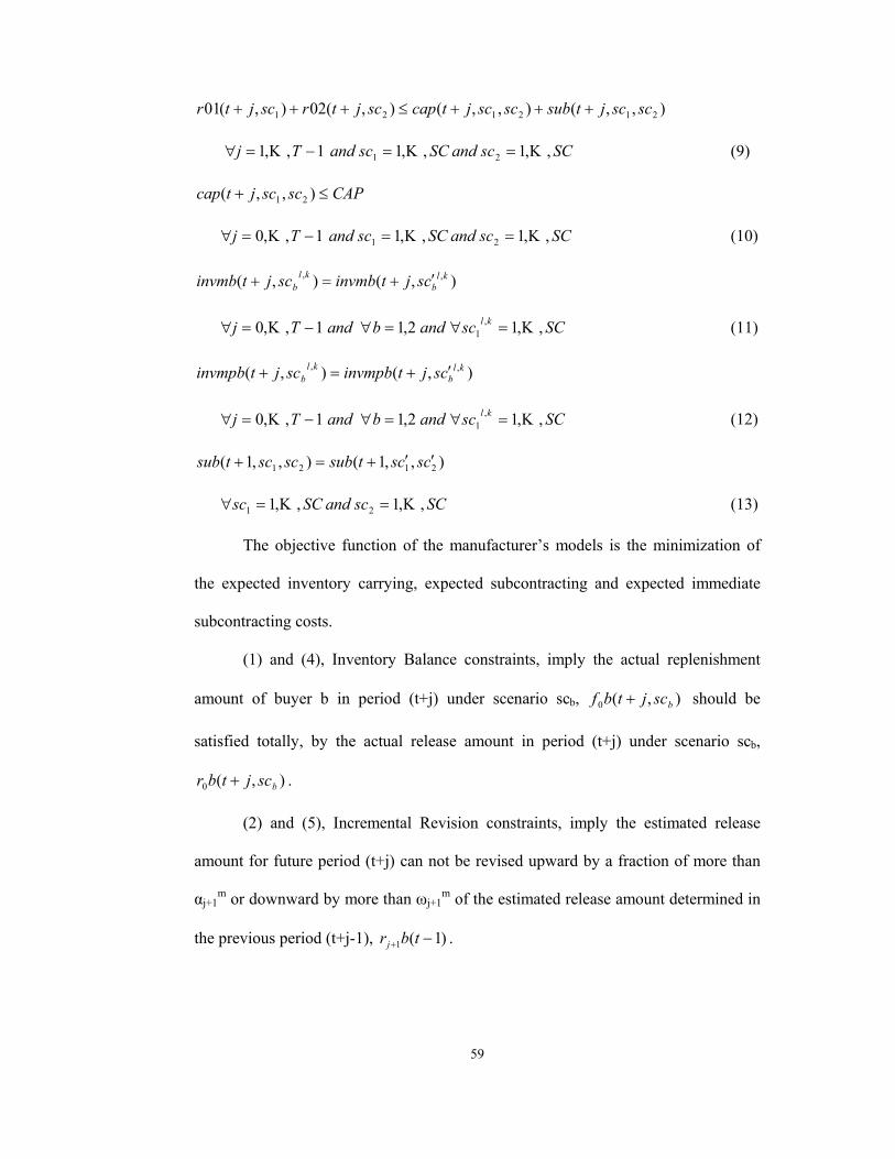
59

),,(),,(),(02),(01 212121 scscjtsubscscjtcapscjtrscjtr +++≤+++

SCscandSCscandTj ,,1,,11,,1 21 ΚΚΚ ==−=∀ (9)

CAPscscjtcap ≤+ ),,( 21

SCscandSCscandTj ,,1,,11,,0 21 ΚΚΚ ==−=∀ (10)

),(),( ,, klb

klb csjtinvmbscjtinvmb ′+=+

SCscandbandTj kl ,,12,11,,0 ,1 ΚΚ =∀=∀−=∀ (11)

),(),( ,, klb

klb csjtinvmpbscjtinvmpb ′+=+

SCscandbandTj kl ,,12,11,,0 ,1 ΚΚ =∀=∀−=∀ (12)

),,1(),,1( 2121 cscstsubscsctsub ′′+=+

SCscandSCsc ,,1,,1 21 ΚΚ ==∀ (13)

The objective function of the manufacturer’s models is the minimization of

the expected inventory carrying, expected subcontracting and expected immediate

subcontracting costs.

(1) and (4), Inventory Balance constraints, imply the actual replenishment

amount of buyer b in period (t+j) under scenario scb, ),(0 bscjtbf + should be

satisfied totally, by the actual release amount in period (t+j) under scenario scb,

),(0 bscjtbr + .

(2) and (5), Incremental Revision constraints, imply the estimated release

amount for future period (t+j) can not be revised upward by a fraction of more than

αj+1m or downward by more than ωj+1

m of the estimated release amount determined in

the previous period (t+j-1), )1(1 −+ tbrj .

60

(3) and (6), Cumulative Flexibility constraints, imply the estimated release

amount for period (t+j) determined in the current period t, )(tbrj , suggests bounds on

the decision for the actual release amount for period (t+j) under scenario scb ,

),(0 bscjtbr + .

(7) Inventory Pooling constraints, imply inventory carrying decisions in

scenario sc1 and sc2 resulting from the satisfaction of the actual replenishment

amounts in scenario sc1 and sc2 are served by the total pooled inventory from which

the required amounts can be released separately.

(8), (9), and (10) Capacity Limitation constraint, imply the sum of the actual

release amounts in period (t+j) under the combination of scenario sc1 and sc2 can not

exceed the capacity limit. We have a costly option to each of the given constant

capacity limit for later periods. Due to the one period lead time subcontracting, the

order given in the period t won’t be on hand until period (t+1).

(11), and (12), Nonanticipativity constraints of the manufacturer, imply

scenarios having a common history have the same set of inventory carrying and

pooling decisions for buyer b to inherit from.

(13), Nonanticipativity constraints for subcontracting decision for period

(t+1), imply the subcontracting decision for the delivery in period

(t+1), ),,( 21 scscjtsub + , should be the same under all combinations of the scenarios

sc1 and sc2, since the order should be given in period t to have delivered in period

(t+1).

61

INTEGRATED SUPPLY CHAIN ENVIRONMENT

An integrated supply chain model, where there is no information asymmetry

between the supply chain actors is constructed. That is to say, in the integrated SC

model, all information about the market demand, intended future replenishment

decisions of the buyers are passed on to the manufacturer, so are the information of

intended future release and subcontracting decisions of the manufacturer to the

buyers. The reason to analyze this case is to see the impacts of the information

sharing on the individual and system wide performance.

For the integrated supply chain model, the scenario trees constructed

separately for each buyer are combined. The random occurrences in integrated SC

model are only at the buyer-market interface. The buyers determine their scenario

based decisions such as actual replenishment amounts, amount of ending inventory

and backordered demand for each period by taking the scenario trees of each one into

account. According to the actual and intended future replenishment amount decisions

of the periods in a given scenario, which are determined by the buyers; the

manufacturer prepares his actual and intended future release amounts, respectively.

Moreover, he determines his amount of ending inventory, inventory pooled and order

to be given to the subcontractor for each period given a scenario.

Integrated Supply Chain Stochastic Model (INTSC-STOCH):

Finally, the integrated supply chain model can be illustrated as below;

Min ∑∑∑= =

−

=

++×++×2

1 1

1

0

]),(),()[(b

SC

sc

T

jbbb

b

scjtbackbbbscjtinvbhbscprobb

∑∑∑=

−

=

++×2

1

1

0

)],()[(b

SC

sc

T

jbb

b

scjtinvmbhmscprobsb

62

∑∑∑ ++×−

=

SC

sc

SC

sc

T

jscscjtsubsmscprobsscprobs

1 2

1

12121 )],,()[(2)(1

∑=

×2

1exp

bbsubsubex

s.t.

Equations (1), (2), (3), and (4) in the formulations of BUY-STOCH1 and BUY-

STOCH2.

Equations (2), (3), (5), (6), (7), (8), (9), (10), (11), (12), and (13) in the formulation

of MAN-STOCH.

),(1),(11exp),1(1),(1 101011 scjtfscjtrsubscjtinvmpscjtinvm +−+++−+=+

SCscandTj ,,11,,0 1 ΚΚ =−=∀ (1)

),(2),(22exp),1(2),(2 202022 scjtfscjtrsubscjtinvmpscjtinvm +−+++−+=+

SCscandTj ,,11,,0 2 ΚΚ =−=∀ (2)

The objective function of the integrated SC model is the minimization of the

expected aggregate inventory carrying and backordering costs of buyers; expected

inventory carrying, subcontracting and immediate subcontracting costs of

manufacturer.

(1) and (2), Inventory Balance constraints of the manufacturer for buyer b,

imply the actual replenishment amount of buyer b in period (t+j) under scenario scb,

),(0 bscjtbf + should be satisfied totally, by the actual release amount in period (t+j)

under scenario scb, ),(0 bscjtbr + . In these constraints, ),(0 bsctbf is the actual

replenishment amount under scenario scb and ),(0 bscjtbf + is the intended future

replenishment amount determined by buyer b, for period (t+j) under scenario scb.

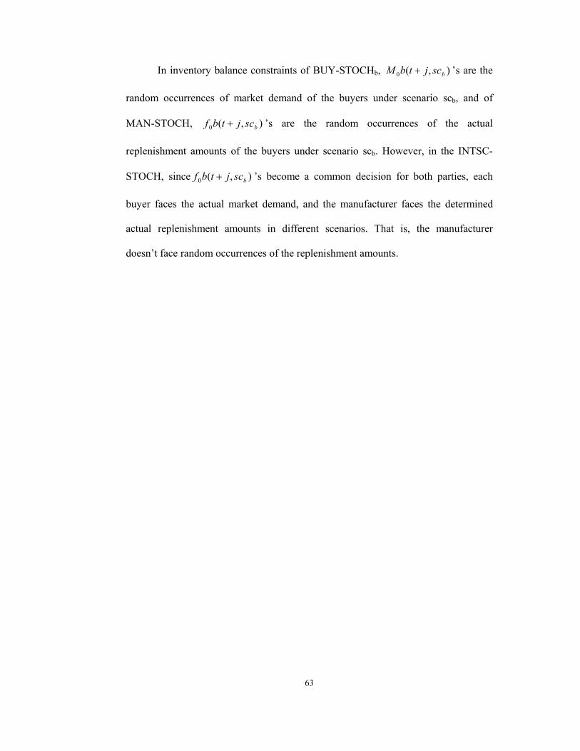
63

In inventory balance constraints of BUY-STOCHb, ),(0 bscjtbM + ’s are the

random occurrences of market demand of the buyers under scenario scb, and of

MAN-STOCH, ),(0 bscjtbf + ’s are the random occurrences of the actual

replenishment amounts of the buyers under scenario scb. However, in the INTSC-

STOCH, since ),(0 bscjtbf + ’s become a common decision for both parties, each

buyer faces the actual market demand, and the manufacturer faces the determined

actual replenishment amounts in different scenarios. That is, the manufacturer

doesn’t face random occurrences of the replenishment amounts.

64

CHAPTER IV

TWO-STAGE STOCHASTIC MODELLING AND SOLUTION

METHOD

The two-stage stochastic programming is chosen as a technique for

formulation, since the decision variables of the problem can be partitioned into two

sets. The first-stage variables correspond to the decisions that need to be made prior

to realization of uncertain demand, are here and now decisions. The replenishment

amount estimates, for the buyers and the estimated release amounts, for the

manufacturer, which are independent of random occurrences and are determined

prior to demand realizations of uncertain demand, are the first stage variables.

Subsequently, based on these estimated replenishment and release decisions and a

given realization of the random demand the second-stage decisions are made wait

and see decisions. That is to say, the actual replenishment and release amounts are

decided in accordance with the values of the first stage variables.

The presence of uncertainty is translated into the stochastic nature of the costs

associated with the second-stage decisions. Therefore, the objective function consists

of the sum of the first-stage decision costs and the expected second-stage recourse

costs. Since all inventory carrying, backordering, actual replenishment, actual release

and subcontracting decision variables are made accordance with a random

realization, they are “wait and see” decision variables. Thus, in all two-stage

65

stochastic programming models for the SC actors, there exist no first stage costs.

This means that both the buyers and the manufacturer are free in their decisions in

the estimates. However, these estimates put bounds on the wait and see decisions, the

actual replenishment and actual release amounts, and so affect the capacity and

subcontracting decisions.

This chapter is organized as follows. In $3.1, the structure of a two-stage

stochastic programming model is introduced. Then, the two-stage stochastic models

for the buyers, the manufacturer, and the integrated supply chain are presented. In

$3.2, the applications of Benders decomposition algorithm for the models presented

in the previous section are displayed.

4.1 TWO STAGE STOCHASTIC MODELS AND BENDERS

DECOMPOSITION

The two-stage stochastic programming model for the buyer b can be

presented as follows;

Min Q

⎥⎥⎥⎥⎥⎥⎥⎥⎥⎥⎥⎥

⎦

⎤

⎢⎢⎢⎢⎢⎢⎢⎢⎢⎢⎢⎢

⎣

⎡

−=∀

Α+≤+≤Ω−

−=∀+−++−+−−+

=+−+

+×++×

=

∑−

=

−++

1,...,0

)()1()()()1(1,...,0

)()()1()1()()(

..

)()(min

0

00

1

1

,)],1(),...1(),([ 000

Tj

tbfjtbftbfTj

jtbjtbfjtbackbjtinvbjtbackbjtinvb

ts

jtbackbbbjtinvbhb

EQ

jbjj

bj

T

j

Tttt µµµµ

66

s.t.

)1()1()()1()1( 1111 −+≤≤−− ++++ tbftbftbf jbjjj

bj αω

2,...,0 −=∀ Tj

The outer problem consists of the first stage variables, that is, the estimated

replenishment amounts, )(tbf j ’s. The inner problem is the recourse function which

is comprised of the second stage variables, that is, the scenario dependent variables.

It is the recourse paid to the overall problem due to the uncertainty. The interaction

between the outer and inner problems takes place through the incremental flexibility

constraints. Our aim is to obtain a closed form for Q (recourse function) in terms of

the first stage variables. This is achieved by solving the inner recourse problem

followed by analytical expectation evaluation. The approach is similar to all other

problems, i.e., problems of the manufacturer and the integrated SC.

The main challenge associated with solving two-stage stochastic problems is

the evaluation of the expectation of the inner recourse problem. For the scenario-

based representation of uncertainty, this can be achieved by explicitly associating a

second-stage variable with each scenario and solving the large-scale formulation by

efficient solution techniques such as Dantzig-Wolfe decomposition and Benders

decomposition.

The stochastic programming model is difficult to solve since the number of

variables and constraints can obviously become very large as the number of

scenarios grows. The number of scenarios, in turn, grows exponentially in terms of

the sample space for random demands. Benders decomposition has been used in

stochastic programming as a method for breaking the model down into small

components that can be analyzed separately. Not only due to this feature of Benders

67

decomposition, but also in order to incorporate the stochastic terms through

expectations by obtaining the closed form of the recourse function, Benders

Decomposition Algorithm is used to solve the stochastic programming models for

SC actors and the integrated supply chain.

In the decomposition algorithm, the stochastic supply chain planning model is

solved iteratively through a sequence of LP sub problems and LP master problems,

with the former minimizing the objective that provides upper bounds (UB) to the

expected total cost. Since some decision variables are taken as given to the sub

problem, it supplies upper bound for the overall problem. The latter providing lower

bounds (LB), minimizes the maximum cut, i.e., LB. The cuts are generated by sum

of the expected total cost suggested by the sub problem and the dualized costs at each

iteration. The dualized costs where the master problem decision variables exist gives

the LB character since it represents the possible reduction from the expected total

cost.

We partition the stochastic LP problem according to the first and second

decision stages stated in the introduction part of this chapter. In the master problem,

the estimated replenishment and release amounts are determined, and then in the sub

problem, the decisions for the actual replenishment by the buyers and release

amounts by the manufacturer, inventory carried, amount backordered and amount

subcontracted are decided. For instance for the first buyer, the master problem

includes all estimated replenishment decisions, )(tbf j ’s which are in fact the “here

and now” decisions determined prior to a realization of the random demand. The sub

problem involves the remaining scenario based decisions; which are actual

replenishment amounts, ),(0 bscjtbf + , amount of ending inventory, ),( bscjtinvb +

68

and amount backordered, ),( bscjtbackb + . That is, the sub problem includes the

“wait and see” decisions which are determined after the realization of the random

demand and according to the predetermined master problem decisions. The sub and

master problems are identical for both buyers.

However, for the manufacturer, the sub problem consists of the scenario

based decisions, i.e. “wait and see” decisions, which are not only actual release

amounts, ),(0 bscjtbr + , inventory carried, ),( bscjtinvmb + , inventory pooled,

),( bscjtinvmpb + , but also includes amount to be ordered from the one period lead

time subcontractor, ),,( 21 scscjtsub + and the same from the immediate

subcontractor, bsubexp . The master model produces the “here and now” decisions,

which are the estimated release decisions, )(tbrj to serve each buyer.

From the buyer’s point of view, the purpose of the master problem is to find

the optimal estimated replenishment decisions, to minimize the expected total cost

transferred from the sub problem prior to the realization of the random demand. The

purpose of the sub problem is to act upon the master problem suggestions, i.e.,

estimated replenishment amounts of the future periods. This is done by evaluating

the expected total cost under the individual scenarios that might occur and determine

the “wait and see” decisions under each scenario. For the manufacturer, the master

problem aims to find the optimal estimated release amounts that will be conveyed on

to the sub problem. Then, the sub problem analyzes the suggestions of the master

problem upon taking all possible scenarios individually each being aggregated over

the buyers.

69

Buyer’s Two-Stage Stochastic Model:

Given any buyer, Nj tbf )( of the master problem decisions in iteration N of

the decomposition algorithm are passed from the master problem to the sub problem.

The sub problem and master problem at iteration N can be stated as follows;

SUB PROBLEM

Min ]),(),()[(1

1

0∑∑

=

−

=

+×++×SC

sc

T

jbbb

b

scjtbackbbbscjtinvbhbscprobb

s.t.

),(),(),1(),1(),(),(

00 bbbb

bb

scjtbMscjtbfscjtbackbscjtinvbscjtbackbscjtinvb

+−++−+−−+=+−+

SCscandTj b ,,11,,0 ΚΚ =∀−=∀ (1)

)()1(),()()1( 0 tbfscjtbftbf jbjbj

bj Α+≤+≤Ω−

SCscandTj b ,,11,,0 ΚΚ =∀−=∀ (2)

),(),( ,, klb

klb csjtinvbscjtinvb ′+=+

SCscandTj klb ,,11,,0 , ΚΚ =∀−=∀ (3)

The objective function of the sub problem of the buyers is the minimization

of the expected inventory carrying and backordering costs over the scenarios.

(2) Cumulative Flexibility constraints imply the estimated replenishment

amount for period (t+j) determined in the master problem, )(tbf j , impose bounds on

the decision for the actual replenishment amount for period (t+j) under any scenario

scb, ),(0 bscjtbf + .

(1) and (3) are the same as the equations (1) and (4) in BUY-STOCHb

described in the previous chapter, respectively.

70

MASTER PROBLEM

Min M

s.t.

)1()1()()1()1( 1111 −+≤≤−− ++++ tbftbftbf jbjjj

bj αω 2,,0 −=∀ Tj Κ (4)

[ ]∑∑=

−

=

++×++×≥SC

sc

T

j

Nb

Nbb scjtbackbbbscjtinvbhbscprobbM

1

1

0)),(()),(()(

∑∑−

= =

++−Α++2

1 10 ]),()()1[()(

T

j

SC

sc

Nbj

bj

Nbsc

b

bscjtbftbfjtUρ

∑∑−

= =

Ω−−++2

1 10 )]()1(),([)(

T

j

SC

scj

bj

Nb

Nbsc

b

btbfscjtbfjtLρ (5)

The objective function of the master problem of the buyers is the

minimization of the maximum cut generated in the sub problem.

(4) is the same as equation (2) in BUY-STOCHb.

In (5), Nbsc jtU

b)( +ρ and Nb

sc jtLb

)( +ρ ‘s are the dual multipliers of the

cumulative flexibility constraints (2) in the sub problem; i.e., of the upper and lower

bounds for the intended future replenishment amounts;

)()1(),(0 tbfscjtbf jbjb Α+≤+ and ),()()1( 0 bj

bj scjtbftbf +≤Ω− , respectively and

Nbscjtbf ),(0 + , N

bscjtinvb ),( + and Nbscjtbackb ),( + are the given optimal

values of the sub problem at iteration N. The master decision variables, which are the

estimated replenishment amounts for period (t+j), )(tbf j ’s, appear in the incremental

revision constraints (4) and second part of (5).

Constraint (5) is the so-called Benders cut, and can be considered as an

aggregate representation of all scenarios on the total cost suggested by the sub

problem decision variables in iteration N. At the beginning, there are no cuts in the

71

master problem, and then they are sequentially added one by one after solving a sub

problem in each iteration. The second buyer has an identical formulation.

Manufacturer’s Two-Stage Stochastic Model:

The manufacturer faces two different random occurrences of actual

replenishment in all the periods. He is informed only of the current period’s actual

replenishment amounts by the buyers through their orders. For other periods, he has

his own inferences on the replenishments concerning the two buyers. The Nj tbr )( ’s

for buyer b determined in the master problem in iteration N is transferred to the sub

problem. The sub problem and master problem of the manufacturer at the iteration N

is presented as follows.

SUB PROBLEM

Min ∑∑∑=

−

=

++×2

1

1

0)],()[(

b

SC

sc

T

jbb

b

scjtinvmbhmscprobsb

∑∑∑ ++×−

=

SC

sc

SC

sc

T

jscscjtsubsmscprobsscprobs

1 2

1

12121 )],,()[(2)(1

∑=

×2

1exp

bbsubsubex

s.t.

),(1),(11exp),1(1),(1 101011 scjtfscjtrsubscjtinvmpscjtinvm +−+++−+=+

SCscandTj ,,11,,0 1 ΚΚ =−=∀ (1)

)(1)1(),(1)(1)1( 110

1 trscjtrtr jmjj

mj Α+≤+≤Ω−

SCscandTj ,,11,,0 1 ΚΚ =−=∀ (2)

),(2),(22exp),1(2),(2 202022 scjtfscjtrsubscjtinvmpscjtinvm +−+++−+=+

72

SCscandTj ,,11,,0 2 ΚΚ =−=∀ (3)

)(2)1(),(2)(2)1( 220

2 trscjtrtr jmjj

mj Α+≤+≤Ω−

SCscandTj ,,11,,0 2 ΚΚ =−=∀ (4)

),(2),(1),(2),(1 2121 scjtinvmpscjtinvmpscjtinvmscjtinvm +++=+++

SCscandSCscandTj ,,1,,11,,0 21 ΚΚΚ ==−=∀ (5)

)(),,(),(02),(01 2121 tSUBscsctcapsctrsctr +≤+

SCscandSCsc ,,1,,1 21 ΚΚ == (6)

),,(),,(),(02),(01 212121 scscjtsubscscjtcapscjtrscjtr +++≤+++

SCscandSCscandTj ,,1,,11,,0 21 ΚΚΚ ==−=∀ (7)

CAPscscjtcap ≤+ ),,( 21

SCscandSCscandTj ,,1,,11,,0 21 ΚΚΚ ==−=∀ (8)

),(),( ,, klb

klb csjtinvmbscjtinvmb ′+=+

SCscandbandTj kl ,,12,11,,0 ,1 ΚΚ =∀=∀−=∀ (9)

),(),( ,, klb

klb csjtinvmpbscjtinvmpb ′+=+

SCscandbandTj kl ,,12,11,,0 ,1 ΚΚ =∀=∀−=∀ (10)

),,1(),,1( 2121 cscstsubscsctsub ′′+=+ SCscandSCsc ,,1,,1 21 ΚΚ ==∀ (11)

The objective function of the sub problem for the manufacturer is the

minimization of the expected inventory carrying, subcontracting and immediate

subcontracting costs over the scenarios.

(2) and (4), Cumulative Flexibility constraints imply the estimated release

amount for period (t+j) determined in master problem, )(tbrj , impose bounds on the

decision for the actual release amount under any scenario scb, ),(0 bscjtbr + .

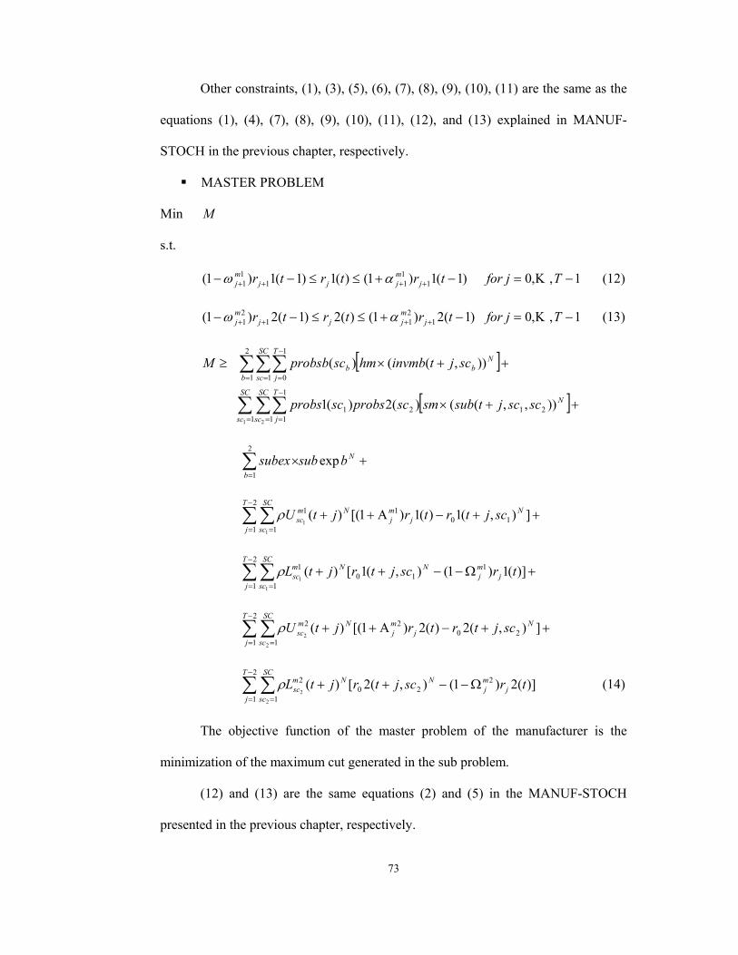
73

Other constraints, (1), (3), (5), (6), (7), (8), (9), (10), (11) are the same as the

equations (1), (4), (7), (8), (9), (10), (11), (12), and (13) explained in MANUF-

STOCH in the previous chapter, respectively.

MASTER PROBLEM

Min M

s.t.

)1(1)1()(1)1(1)1( 1111

11 −+≤≤−− ++++ trtrtr j

mjjj

mj αω 1,,0 −= Tjfor Κ (12)

)1(2)1()(2)1(2)1( 1211

21 −+≤≤−− ++++ trtrtr j

mjjj

mj αω 1,,0 −= Tjfor Κ (13)

[ ]

[ ]∑ ∑∑

∑∑∑

= =

−

=

= =

−

=

++×

++×≥

SC

sc

SC

sc

NT

j

b

SC

sc

T

j

Nbb

scscjtsubsmscprobsscprobs

scjtinvmbhmscprobsbM

1 1212

1

11

2

1 1

1

0

1 2

)),,(()(2)(1

)),(()(

+×∑=

N

bbsubsubex exp

2

1

∑∑−

= =

++−Α++2

1 110

11

1

1]),(1)(1)1[()(

T

j

SC

sc

Nj

mj

Nmsc scjtrtrjtUρ

∑∑−

= =

+Ω−−++2

1 1

110

1

1

1)](1)1(),(1[)(

T

j

SC

scj

mj

NNmsc trscjtrjtLρ

∑∑−

= =

++−Α++2

1 120

22

2

2]),(2)(2)1[()(

T

j

SC

sc

Nj

mj

Nmsc scjtrtrjtUρ

∑∑−

= =

Ω−−++2

1 1

220

2

2

2)](2)1(),(2[)(

T

j

SC

scj

mj

NNmsc trscjtrjtLρ (14)

The objective function of the master problem of the manufacturer is the

minimization of the maximum cut generated in the sub problem.

(12) and (13) are the same equations (2) and (5) in the MANUF-STOCH

presented in the previous chapter, respectively.

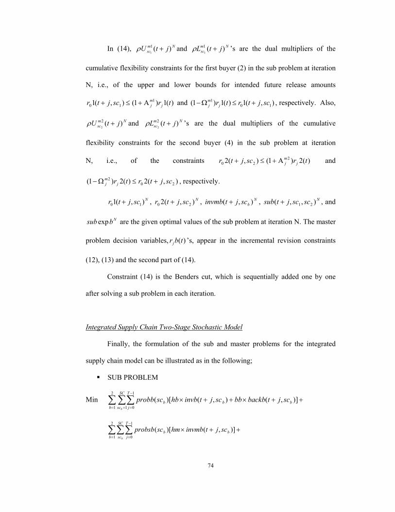
74

In (14), Nmsc jtU )(1

1+ρ and Nm

sc jtL )(11

+ρ ’s are the dual multipliers of the

cumulative flexibility constraints for the first buyer (2) in the sub problem at iteration

N, i.e., of the upper and lower bounds for intended future release amounts

)(1)1(),(1 110 trscjtr j

mjΑ+≤+ and ),(1)(1)1( 10

1 scjtrtrjmj +≤Ω− , respectively. Also,

Nmsc jtU )(2

2+ρ and Nm

sc jtL )(22

+ρ ’s are the dual multipliers of the cumulative

flexibility constraints for the second buyer (4) in the sub problem at iteration

N, i.e., of the constraints )(2)1(),(2 220 trscjtr j

mjΑ+≤+ and

),(2)(2)1( 202 scjtrtrj

mj +≤Ω− , respectively.

Nscjtr ),(1 10 + , Nscjtr ),(2 20 + , Nbscjtinvmb ),( + , Nscscjtsub ),,( 21+ , and

Nbsub exp are the given optimal values of the sub problem at iteration N. The master

problem decision variables, )(tbrj ’s, appear in the incremental revision constraints

(12), (13) and the second part of (14).

Constraint (14) is the Benders cut, which is sequentially added one by one

after solving a sub problem in each iteration.

Integrated Supply Chain Two-Stage Stochastic Model

Finally, the formulation of the sub and master problems for the integrated

supply chain model can be illustrated as in the following;

SUB PROBLEM

Min ∑∑∑= =

−

=

++×++×2

1 1

1

0]),(),()[(

b

SC

sc

T

jbbb

b

scjtbackbbbscjtinvbhbscprobb

∑∑∑=

−

=

++×2

1

1

0)],()[(

b

SC

sc

T

jbb

b

scjtinvmbhmscprobsb

75

∑∑∑ ++×−

=

SC

sc

SC

sc

T

jscscjtsubsmscprobsscprobs

1 2

1

12121 )],,()[(2)(1

∑=

×2

1exp

bbsubsubex

s.t

Equations (1), (2), and (3) in the sub problems of each buyer

Equations (2), (3), (4), (6), (7), (8), (9), (10), and (11) in the sub problem of the

manufacturer

),(1),(11exp),1(1),(1 101011 scjtfscjtrsubscjtinvmpscjtinvm +−+++−+=+

SCscandTj ,,11,,0 1 ΚΚ =−=∀ (1)

),(2),(22exp),1(2),(2 202022 scjtfscjtrsubscjtinvmpscjtinvm +−+++−+=+

SCscandTj ,,11,,0 2 ΚΚ =−=∀ (2)

The objective function of the integrated supply chain model is the

combination of the objective function in the buyers’ and manufacturer’s sub

problems.

(1) and (2), Inventory Balance constraints of the manufacturer for buyer b

imply the actual replenishment amount of buyer b in period (t+j) under scenario scb

should be satisfied totally, by the actual release amount in period (t+j) under scenario

scb, ),(0 bscjtbr + . In these constraints, ),(0 bsctbf is the actual replenishment

amount under scenario scb and ),(0 bscjtbf + is the intended future replenishment

amount determined by buyer b, for period (t+j) under scenario scb.

MASTER PROBLEM

Min M

s.t.

76

Equations (4) in the master problems of each buyer

Equations (12) and (13) in the master problem of the manufacturer

[ ]∑∑∑= =

−

=

++×++≥2

1 1

1

0)),(()),(()(

b

SC

sc

T

j

Nb

Nbb scjtbackbbbscjtinvbhbscprobbM

[ ]∑∑∑= =

−

=

++×2

1 1

1

0)),(()(

b

SC

sc

T

j

Nbb scjtinvmbhmscprobsb

[ ]∑ ∑∑= =

−

=

++×SC

sc

SC

sc

NT

jscscjtsubsmscprobsscprobs

1 1212

1

11

1 2

)),,(()(2)(1

+×∑=

N

bbsubsubex exp

2

1

∑ ∑∑=

−

= =⎩⎨⎧

++−Α++2

1

2

1 10 ]),()()1[()(

b

T

j

SC

sc

Nbj

bj

Nbsc

b

bscjtbftbfjtUρ

+⎭⎬⎫

Ω−−++∑∑−

= =

2

1 10 )]()1(),([)(

T

j

SC

scj

bj

Nb

Nbsc

b

btbfscjtbfjtLρ

∑ ∑∑=

−

= =⎩⎨⎧

++−Α++2

1

2

1 10 ]),()()1[()(

b

T

j

SC

sc

Nbj

mbj

Nmbsc

b

bscjtbrtbrjtUρ

⎭⎬⎫

Ω−−++∑ ∑−

= =

2

1 10

1

)]()1(),([)(T

j

SC

scj

mbj

Nb

Nmbsc

b

btbrscjtbrjtLρ (3)

The objective function of the master problem of the integrated supply chain is

the minimization of the maximum cut generated in the sub problem.

In (3), Nbsc jtU

b)( +ρ , Nb

sc jtLb

)( +ρ and Nmbsc jtU

b)( +ρ , Nmb

sc jtLb

)( +ρ ’s are the

dual multipliers of the cumulative flexibility constraints of each buyer and of the

manufacturer for each buyer in their sub problems, Nbscjtbf ),(0 + and,

Nbscjtbr ),(0 + , N

bscjtinvb ),( + , Nbscjtbackb ),( + , N

bscjtinvmb ),( + ,

77

Nscscjtsub ),,( 21+ , and Nbsub exp are the given optimal values of the sub problem

at iteration N.

Constraint (3) is the Benders cut which is consecutively added one by one

after solving a sub problem in each iteration.

4.2 BENDERS DECOMPOSITION ALGORITHM

Our main interest is to solve the two-sage stochastic programming models.

Thus, we utilize Benders Decomposition algorithm, where the stochastic model is

solved iteratively through a sequence of LP sub problems and LP master problems

and which guarantees convergence.

The algorithm for the buyers can be presented as follows;

Step 1 Set N to 1. Select Ntbf )(1 from WCP. Set UB= +infinity and LB= -

infinity

Step 2 Solve Sub Problem(N)

Step 2.1 Update the upper bound by setting UB=minUB, expected total costN

Step 3 Solve the Master Problem(N) to determine 11 )( +Ntbf and a lower

bound to total cost. Set LB equal to the solution of this Master

Problem(N)

Step 4 If UB-LB < tolerance, stop. Otherwise, set N=N+1, and go to Step 2.

In Benders decomposition algorithm for the manufacturer, Ntbf )(1 is

replaced by Ntbr )(1 which is found by solving WCP of the manufacturer. The

expected total cost at iteration N is comprised of the Nbscjtbr ),(0 + ,

78

Nbscjtinvmb ),( + , N

bscjtinvmpb ),( + and Nscscjtsub ),,( 21+ . The steps to follow

are the same as in the buyer’s case.

In step 1 of both algorithm applications, the initial values, 1)(tbf j and 1)(tbrj

can be obtained by solving, what we called “the worst case problem” (WCP). WCP

is acquired by replacing each random market demand and each random

replenishment amount by its worst scenario, that is, by the largest amount of possible

demand and replenishment values of each period. By this way, the estimated

replenishment and release amounts are initially determined as if the biggest value of

the demand or replenishment is realized, respectively.

At the beginning, the WCP is selected to employ for the manufacturer in

order not to generate such estimated release amounts that will be short of satisfying

the total actual replenishment amounts for the two buyers. That is, not to get into

infeasibility in inventory balance constraints of the manufacturer for the buyers

individually in the sub problem. Although, there is no possibility to get into

infeasibility in inventory balance constraints of the two buyers due to allowing for

backorders, to be consistent for all the SC actors, the WCP is employed also in the

buyer’s case.

The Benders decomposition algorithm for the buyers can be illustrated in

Figure 4.1. First by the worst case problem (WCP), the initial optimal estimated

replenishment amounts are determined. Then, they are input to the sub problem.

After taking the suggestions of the WCP into consideration, the sub problem

determines the actual replenishment amounts, inventory carrying and backordering

amounts in expected value terms, considering all scenarios. The expected total cost

found in each optimization of the sub problem supplies a new upper bound (UB) for

79

the overall problem. The new UB found at each iteration should be less than or equal

to the UB found at the previous iteration. This is due not to make an iteration which

is not close to the optimal solution with respect to the solution of the previous

iteration and to reduce the gap between the UB and LB more efficiently. Afterwards,

the expected total cost, and the most recent optimal values of the sub problem

decisions are transferred to the master problem. New optimal estimated

replenishment amounts are determined in the master problem, where the optimal

objective function value establishes a lower bound (LB) for the overall problem. The

main problem takes all previously generated LB’s into account. Since a new cut is

added to the master problem at each iteration, the new LB is found on minimizing

the maximum cut, i.e., LB. Thus, the algorithm tightens the lower bounds iteratively.

When the gap between UB and LB is less than a predetermined tolerance (0.0001),

the problem is said to be solved with sufficient accuracy.

Figure 4.1 Benders Decomposition Algorithm

The figure of the algorithm for the manufacturer is not presented, since it has

the same approach with the buyers’.

Master Problem

Sub Problem

Supplies LB and a Replenishment Schedule.

1)( +Nj tbf ’s are

transferred

Supplies UB and Expected total cost expressions over scenarios dependent on the Replenishment Schedule.

Nbscjtbf ),(0 + , N

bscjtinvb ),( + , N

bscjtbackb ),( + ’s are transferred

Initialization (WCP)

Terminate

80

The Benders cut stated above assumes that all sub problems are feasible.

However, the trial points generated by the master problem may not necessarily be

feasible for all realizations of the random parameters. An approach appropriate for

this supply chain planning problem, which is adding feasibility constraints to the

master problem, is taken into account for implementation.

The feasibility constraints for the buyers are presented below.

10

1 )()1(),()()1( ++ Α+≤+≤Ω− Nj

bj

Nb

Nj

bj tbfscjtbftbf

SCscandTj b ,,12,,1 ΚΚ =−=∀ (1)

For the buyer’s case, the above formulation implies the new optimal

estimated replenishment amounts generated by the master problem at iteration N;

construct such bounds that they should cover at least the actual replenishment

amount values in any scenario scb predetermined in the sub problem at iteration N.

For the manufacturer’s case, only the estimated replenishment and

predetermined actual replenishment amounts are replaced by estimated release and

predetermined actual release amounts, respectively.

Although the loop terminates due to the achievement of satisfactory

convergence, the estimated replenishment and estimated release amounts can take

such values that they can make the sub problem infeasible. By the feasibility

constraints presented above, the stated case is prevented.

In our analysis, specifically, given the capacity limit and the release schedule

of the first buyer, after introducing the second buyer, the capacity planning issue of

the manufacturer and the effect of the contract parameters specified by the second

buyer herself are tried to be examined.

81

In this study, we try to address the objectives; to provide a structure for the

analysis of quantity flexibility contracts, with the assumption of stationary and

uncertain market demand that seeks the challenge for flexibility; suggest forecasting

and ordering policies, for buyers who are obliged to purchase a certain amount of

their estimates, for manufacturer who guarantees to provide a certain amount of the

buyer’s replenishment amounts; and link these behaviors to individual and system

wide performance, so guide the negotiation of contracts.

82

CHAPTER V

EXPERIMENT

This study is based mainly on the incentives of the second buyer who is

offered a QF contract by a manufacturer, and the incentives of the manufacturer

offering a QF contract to the second buyer while he has an active QF contract with

another buyer.

We try to analyze the causes and effects for the attitudes of the Supply Chain

(SC) actors individually and their attitudes in the integrated supply chain with the

environment forming these attitudes. We intend to find out answers to some research

questions such as how much flexibility the manufacturer can tolerate without any

increase in costs, how the choice of flexibility is affected by demand variability, and

how much the manufacturer’s own capacity is utilized in the presence of prior

commitments.

This chapter states why demand variation, flexibility tightness and cost are

selected as the three main factors, and how the levels and the values for these levels

are effective. In $5.1, the definition of the factors for the analysis and their

determined levels are presented. In $5.2, the approach taken for data generation is

displayed. In $5.3, how the samples for the full factorial experiment are created is

stated. Finally, in $5.4, an example for the General Algebraic Modeling Systems

83

(GAMS) utilization and the application of Benders Decomposition algorithm are

presented.

5.1 EXPERIMENTAL FACTORS

In order to carry out our analysis for the effect of a QF contract, its usage, its

options offered to all the parties in the supply chain environment, the individual and

systemwide attitudes of SC actors, we construct a full factorial experiment. For the

experiment, three factors are specified, which are demand variation, flexibility

tightness requested and offered, and cost rates. By the full factorial experiment, we

try to discover all causes and effects of the events established by changing all

possible levels of the experimental factors determined.

The demand variation is selected as a factor to experiment with in order to

examine the effect of variation on the usage of quantity flexibility option. The option

of quantity flexibility means whether the SC actor takes advantage of the upward or

downward flexibility. In other words, when a larger amount of demand than expected

occurs, the buyer can replenish up to her upper bound set by her estimation in the

previous period. When the opposite occurs, she can replenish less than her estimation

made similarly.

The experimental factor, demand variation (DEVAR), is defined as the

coefficient of variation of the discrete demand values that can occur in a period. The

coefficient of variation is a way to express the variation as a fraction of the mean. It

is useful when comparing variability of two or more data sets that differ considerably

in their observations.

84

We try two levels which are medium and high variation based on the

coefficient of variation. In our full factorial experiment, we aim to analyze at which

amount the flexibility option is required or at which amount the effect of flexibility is

effective in different situations with the factor, DEVAR, set at levels medium or

high. Moreover, the distribution of the benefits among the SC actors in the

decentralized and centralized environments, and the system wide performance at

different levels of demand variation are examined.

Flexibility tightness (FLEX) is chosen as the second factor. Flexibility

tightness is defined by rigidity of the flexibility offered or requested. The tightness of

flexibility has two levels namely tight and loose flexibility. By the selection of the

flexibility tightness as a factor, we intend to analyze the attitudes of the SC actors in

the individual and in the integrated SC environments. Especially, in the integrated

SC, when the tightness of flexibility is changed for a party, whether the option

provides an overall benefit only to that party or to other parties is investigated. We

also try to examine the usage of flexibility when the actors face with different

demand values. For instance, when the buyer faces a high demand, her attitude when

she is given a tight or loose flexibility option and the reason of her attitude are

questioned. For the first case, where the flexibility parameters are determined by the

second buyer; the first buyer and the manufacturer have their own set of defined

flexibility parameters. The flexibility of the first buyer can be tight or loose and those

of the manufacturer can as well be tight or loose. Taking the combinations of the two

parties into account, this factor has four levels for the analysis. In the second case

where the manufacturer determines his quantity flexibility parameters for the second

buyer, the first buyer is given the loose flexibility level determined in the first case.

85

Then, there will be again four combinations to examine for the second buyer and the

manufacturer.

Our final factor is the cost, specifically the costs of inventory carrying,

backordering, subcontracting and immediate subcontracting, (COST). This factor has

two levels, which are low and high cost. In the determining the values of inventory

carrying, backordering costs, etc., we intend to generate four different situations

where the cost burden is transferred first on none of the parties, then only on the

manufacturer, then only on the buyers, and finally, on all. That is, similar to FLEX,

this factor has four combinations, which include the combination of the low and high

unit cost components of the two buyers and the low and high cost of the

manufacturer. The inventory carrying costs of the two buyers and the manufacturer

are taken as the same. Other costs are determined relative to the inventory carrying

cost taken as a base. The burden on the buyers is handled by increasing the

backordering costs of the buyers. By increasing the subcontracting and immediate

subcontracting costs, the manufacturer is given the burden of the cost. By the cost

factor, we try to find answers to the questions; who gets the most benefit, and

whether the attitudes of the SC actors differ in the individual and coordinated

environments. These are studied under the conditions where the cost burden is

transferred onto different parties.

5.2 DATA GENERATION

The effects of the environmental characteristics consisting of the relations

between the actors, the information shared by the parties, the type of the demand

86

they face with, the quantity flexibility parameters specified, and the cost parameters

that applies are investigated. We make our experiment by taking a rolling planning

horizon of 4 periods. 4 periods is appropriate for our analysis since subcontracting

lead time is one period and we want to see the effects of lead time, also we aim to

observe the rolling horizon fashion and the two buyers’ planned inventories and their

utilizations of the flexibility options provided. Our approach is to give minimum and

maximum values for the factor levels such as medium and high DEVAR, tight and

loose FLEX, and low and high COST. For the analysis, the two-stage stochastic

models presented in the previous chapter are constructed with the specified demand

variation, flexibility tightness and cost factor levels.

5.2.1 GENERATION OF FACTOR LEVELS

In order to carry out our full factorial experiment, we first define values for

the levels of the experimental factors. Then, to obtain the numerical results for the

specified analysis, we generate the data to be utilized in the two-stage stochastic

models constructed in the previous chapter.

DEMAND VARIATION

For the factor of DEVAR, the logic is based on coefficient of variation (CV).

For the levels, medium and high DEVAR, the CV values tested can be seen in the

Table 5.1.

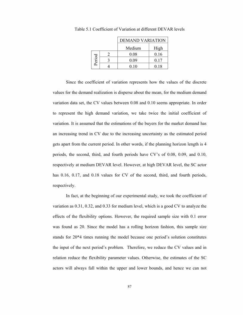
87

Table 5.1 Coefficient of Variation at different DEVAR levels

DEMAND VARIATION

Medium High 2 0.08 0.16 3 0.09 0.17

Perio

d

4 0.10 0.18

Since the coefficient of variation represents how the values of the discrete

values for the demand realization is disperse about the mean, for the medium demand

variation data set, the CV values between 0.08 and 0.10 seems appropriate. In order

to represent the high demand variation, we take twice the initial coefficient of

variation. It is assumed that the estimations of the buyers for the market demand has

an increasing trend in CV due to the increasing uncertainty as the estimated period

gets apart from the current period. In other words, if the planning horizon length is 4

periods, the second, third, and fourth periods have CV’s of 0.08, 0.09, and 0.10,

respectively at medium DEVAR level. However, at high DEVAR level, the SC actor

has 0.16, 0.17, and 0.18 values for CV of the second, third, and fourth periods,

respectively.

In fact, at the beginning of our experimental study, we took the coefficient of

variation as 0.31, 0.32, and 0.33 for medium level, which is a good CV to analyze the

effects of the flexibility options. However, the required sample size with 0.1 error

was found as 20. Since the model has a rolling horizon fashion, this sample size

stands for 20*4 times running the model because one period’s solution constitutes

the input of the next period’s problem. Therefore, we reduce the CV values and in

relation reduce the flexibility parameter values. Otherwise, the estimates of the SC

actors will always fall within the upper and lower bounds, and hence we can not

88

observe the conditions where the flexibility options are used effectively and where

they are inadequate.

FLEXIBILITY TIGHTNESS

For the factor FLEX, the level values are determined in such a way that they

give the opportunity to all SC parties to exploit the flexibility option. They are found

by performing some pilot runs, and examining the attitudes of the SC actors in the

specified environment. In the tight flexibility level of the first buyer and the

manufacturer, they are given the flexibilities which provide the SC actors to utilize

the bounds constructed. However, in the loose flexibility level, the estimates by the

actors can fall within the bounds; consequently they carry limited inventory or

backorder less. We expect to see the effect of the flexibility tightness mainly at high

DEVAR level.

According to the model presented in the study by Tsay and Lovejoy (1999),

one of the specifications of their proposition is that the flexibility parameters of the

upstream party should not be less than the flexibility parameters of the downstream

parties. They showed that by the proposition, a party which has more flexibility in its

supply process than it offers its customers can meet all obligations with zero

inventory. They state that when the opposite occurs, the party will absorb the

flexibility with no benefit to the system. Therefore, the flexibility parameters of the

manufacturer for the first and second buyers are determined relative to theirs. When

the second buyer determines her contract parameters, the manufacturer settles on his

own flexibility parameters in the same proportion obtained by dividing the tight

flexibility parameter of the manufacturer for the first buyer by the tight flexibility of

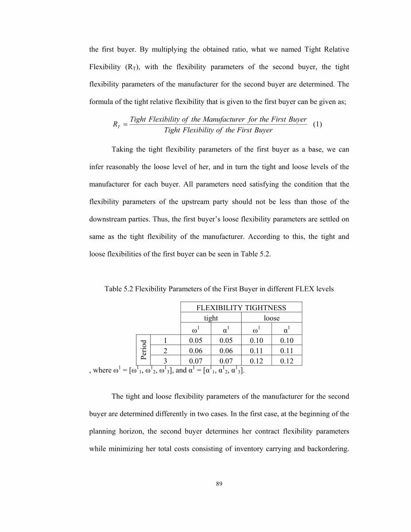
89

the first buyer. By multiplying the obtained ratio, what we named Tight Relative

Flexibility (RT), with the flexibility parameters of the second buyer, the tight

flexibility parameters of the manufacturer for the second buyer are determined. The

formula of the tight relative flexibility that is given to the first buyer can be given as;

BuyerFirsttheofyFlexibilitTightBuyerFirsttheforerManufacturtheofyFlexibilitTightRT = (1)

Taking the tight flexibility parameters of the first buyer as a base, we can

infer reasonably the loose level of her, and in turn the tight and loose levels of the

manufacturer for each buyer. All parameters need satisfying the condition that the

flexibility parameters of the upstream party should not be less than those of the

downstream parties. Thus, the first buyer’s loose flexibility parameters are settled on

same as the tight flexibility of the manufacturer. According to this, the tight and

loose flexibilities of the first buyer can be seen in Table 5.2.

Table 5.2 Flexibility Parameters of the First Buyer in different FLEX levels

FLEXIBILITY TIGHTNESS tight loose ω1 α1 ω1 α1

1 0.05 0.05 0.10 0.10 2 0.06 0.06 0.11 0.11

Perio

d

3 0.07 0.07 0.12 0.12 , where ω1 = [ω1

1, ω12, ω1

3], and α1 = [α11, α1

2, α13].

The tight and loose flexibility parameters of the manufacturer for the second

buyer are determined differently in two cases. In the first case, at the beginning of the

planning horizon, the second buyer determines her contract flexibility parameters

while minimizing her total costs consisting of inventory carrying and backordering.

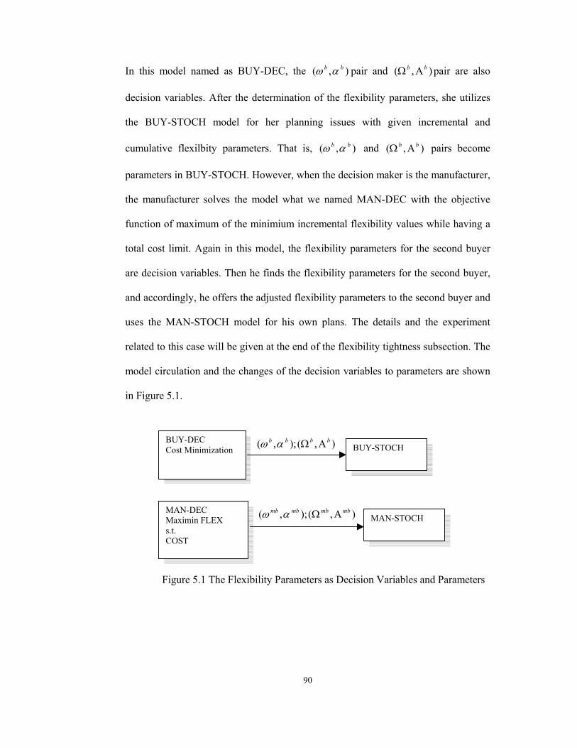
90

In this model named as BUY-DEC, the ),( bb αω pair and ),( bb ΑΩ pair are also

decision variables. After the determination of the flexibility parameters, she utilizes

the BUY-STOCH model for her planning issues with given incremental and

cumulative flexilbity parameters. That is, ),( bb αω and ),( bb ΑΩ pairs become

parameters in BUY-STOCH. However, when the decision maker is the manufacturer,

the manufacturer solves the model what we named MAN-DEC with the objective

function of maximum of the minimium incremental flexibility values while having a

total cost limit. Again in this model, the flexibility parameters for the second buyer

are decision variables. Then he finds the flexibility parameters for the second buyer,

and accordingly, he offers the adjusted flexibility parameters to the second buyer and

uses the MAN-STOCH model for his own plans. The details and the experiment

related to this case will be given at the end of the flexibility tightness subsection. The

model circulation and the changes of the decision variables to parameters are shown

in Figure 5.1.

Figure 5.1 The Flexibility Parameters as Decision Variables and Parameters

BUY-DEC Cost Minimization BUY-STOCH ),();,( bbbb ΑΩαω

MAN-DEC Maximin FLEX s.t. COST

MAN-STOCH ),();,( mbmbmbmb ΑΩαω

91

The decision process of the flexibility parameters of the second buyer and the

manufacturer, and the interaction between the two SC actors are presented in Figure

5.2.

Figure 5.2 Decision Process of the Second Buyer and its Interactions

The second buyer decides both the incremental and cumulative flexibility

parameters which are utilized for her medium and short term decisions. The

downward arc represents the interaction between the second buyer and the

manufacturer. That is, the values of the parameters determined provide the lower and

upper bounds for the replenishment amounts to be requested from the manufacturer.

The manufacturer’s tight and loose flexibility parameters are settled on by

multiplying the parameters of the second buyer with RT and RL, respectively. Since

the tight flexibility of the first buyer is taken as a base, the RL, i.e., the Loose

Relative Flexibility, can be defined as follows;

Second Buyer

Manufacturer

Incremental Flexibility parameters of the Second Buyer, ),( 22 αω Cumulative

Flexibility parameters of the Second Buyer,

),( 22 ΑΩ

Cumulative Flexibility parameters of the Manufacturer,

),( 22 mm ΑΩ

Incremental Flexibility parameters of the Manufacturer, ),( 22 mm αω

Cumulative Flexibility parameters of the Second Buyer, ),( 22 ΑΩ

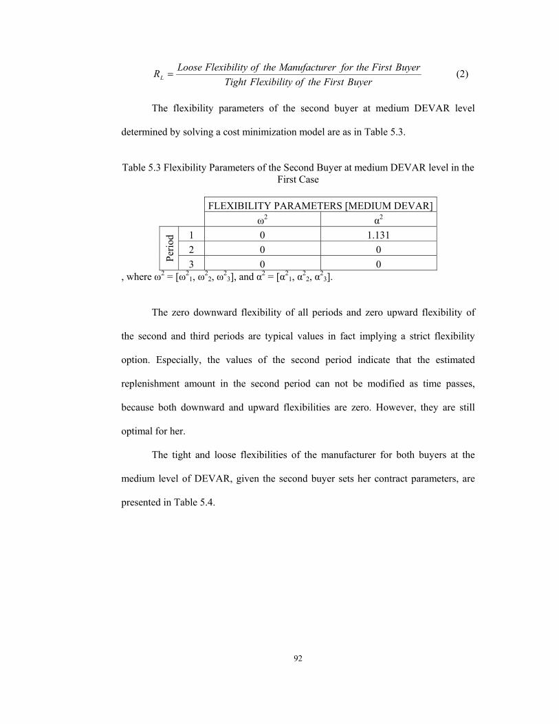
92

BuyerFirsttheofyFlexibilitTightBuyerFirsttheforerManufacturtheofyFlexibilitLooseRL = (2)

The flexibility parameters of the second buyer at medium DEVAR level

determined by solving a cost minimization model are as in Table 5.3.

Table 5.3 Flexibility Parameters of the Second Buyer at medium DEVAR level in the

First Case

FLEXIBILITY PARAMETERS [MEDIUM DEVAR] ω2 α2

1 0 1.131 2 0 0

Perio

d

3 0 0 , where ω2 = [ω2

1, ω22, ω2

3], and α2 = [α21, α2

2, α23].

The zero downward flexibility of all periods and zero upward flexibility of

the second and third periods are typical values in fact implying a strict flexibility

option. Especially, the values of the second period indicate that the estimated

replenishment amount in the second period can not be modified as time passes,

because both downward and upward flexibilities are zero. However, they are still

optimal for her.

The tight and loose flexibilities of the manufacturer for both buyers at the

medium level of DEVAR, given the second buyer sets her contract parameters, are

presented in Table 5.4.

93

Table 5.4 Flexibility Parameters of the Manufacturer at medium DEVAR level and in different FLEX levels in the First Case

FLEXIBILITY TIGHTNESS [MEDIUM DEVAR] SECOND BUYER DETERMINES HER CONTRACT PARAMETERS for FIRST BUYER for SECOND BUYER tight loose tight loose ωm1 αm1 ωm1 αm1 ωm2 αm2 ωm2 αm2

1 0.1 0.1 0.2 0.2 0.05 1.23 0.16 1.44 2 0.11 0.11 0.21 0.21 0.05 0.05 0.16 0.14

Perio

d

3 0.12 0.11 0.22 0.22 0.05 0.05 0.16 0.14 , where ωm1 = [ωm1

1, ωm12, ωm1

3], and αm1 = [αm11, αm1

2, αm13]; and ωm2 = [ωm2

1, ωm22,

ωm23], and αm2 = [αm2

1, αm22, αm2

3].

The incremental flexibilities of the manufacturer for the second buyer are

determined by multiplying the flexibility values determined by the second buyer with

RT and RL for tight and loose levels, respectively. Therefore, in this case, first the

second buyer determines her parameters, and then the manufacturer does.

The flexibility parameters of the second buyer at high DEVAR level are as in

Table 5.5.

Table 5.5 Flexibility Parameters of the Second Buyer at high DEVAR level in the

First Case

FLEXIBILITY PARAMETERS [HIGH DEVAR] ω2 α2

1 0 1.24 2 0 0

Perio

d

3 0 0.044 , where ω2 = [ω2

1, ω22, ω2

3], and α2 = [α21, α2

2, α23].

In high DEVAR, it is observed that the second buyer tries to have higher

flexibility values with respect to medium level. However, the zero value of the

94

downward flexibilities of all periods does not change meaning that they are still

optimal for her.

The tight and loose flexibility parameters of the manufacturer for the high

level of the factor DEVAR, for the second buyer’s offering her contract parameters,

is presented in Table 5.6.

Table 5.6 Flexibility Parameters of the Manufacturer in high DEVAR level and in

different FLEX levels in the First Case

FLEXIBILITY TIGHTNESS [HIGH DEVAR] SECOND BUYER DETERMINES HER CONTRACT PARAMETERS for FIRST BUYER for SECOND BUYER tight loose tight loose ωm1 αm1 ωm1 αm1 ωm2 αm2 ωm2 αm2

1 0.1 0.1 0.2 0.2 0.05 1.35 0.16 1.56 2 0.11 0.11 0.21 0.21 0.05 0.05 0.16 0.14

Perio

d

3 0.12 0.11 0.22 0.22 0.05 0.09 0.16 0.19 , where ωm1 = [ωm1

1, ωm12, ωm1

3], and αm1 = [αm11, αm1

2, αm13]; and ωm2 = [ωm2

1, ωm22,

ωm23], and αm2 = [αm2

1, αm22, αm2

3].

In the second case, the manufacturer determines first his own flexibility

parameters, and then the parameters to be offered to the second buyer. The

manufacturer first intends to offer such contract flexibility parameters that they will

be appealing to the second buyer in order to involve her into the supply chain game.

The second buyer’s flexibility parameters are settled on by dividing the determined

parameters of the manufacturer by the tight relative flexibility, RT stated in the first

case.

Since the cumulative flexibility parameters, Ω andΑ ’s, are formed from the

incremental flexibility parameters, ω andα ’s, we compute only the incremental

flexibility parameters in our analysis. We try to maximize the least incremental

95

flexibility parameter to be offered to the second buyer. However, this is related to the

cost which is comprised of the inventory carrying and subcontracting costs of the

manufacturer.

We first find the minimum total cost in the Worst Case Problem, while not

taking the choice of the flexibility parameters into account. This is achieved by

solving the initial model where the largest replenishment amounts are included.

Then, we include the optimal WCP cost as a total cost constraint to the other problem

where the lowest incremental flexibility parameters are maximized.

We try to see the effect of the flexibility parameters offered to the second

buyer on the manufacturer. Thus, instead of writing the maximum of the possible

replenishment occurrences into the WCP, we include the largest amount possible that

can be requested by the second buyer from the manufacturer given the opportunity of

the QF contract. This critical amount is the upper bound formed by the estimated

replenishment amount in the previous period times the cumulative flexibility,

i.e., )1( 2jΑ+ . The j

2Α ‘s are found by dividing the flexibility parameters of the

manufacturer for the second buyer by the tight relative flexibility, RT that is given to

the first buyer.

We see that when the constraint setting an upper bound to the total cost of

WCP is relaxed, the flexibility parameters increase. That is, there is a tradeoff

between the total cost to the manufacturer and flexibility offered to the second buyer.

We make some pilot runs to examine the effect of the total cost limitation on the

flexibility.

96

Table 5.7 Total Cost versus Downward Incremental Flexibility

Downward Incremental Flexibility 1st Period 2nd Period 3rd Period

2010 0.068 0.068 0.068

2050 0.073 0.073 0.073

2100 0.08 0.08 0.08

2400 0.12 0.155 0.144 B

ound

on

Tota

l Cos

t

on th

e M

anuf

actu

rer

2700 0.158 0.737 0.158

Total Cost vs Downward Incremental Flexibility

0

0,1

0,2

0,3

0,4

0,5

0,6

0,7

0,8

2010 2050 2100 2400 2700Total Cost

Dow

nwar

d In

crem

enta

l Fl

exib

ility 1st Period

2nd Period

3rd Period

Figure 5.3 Total Cost versus Downward Incremental Flexibility Graph

Table 5.8 Total Cost versus Upward Incremental Flexibility

Upward Incremental Flexibility 1st Period 2nd Period 3rd Period

2010 0.068 0.068 0.068

2050 0.073 0.073 0.073

2100 0.08 0.08 0.08

2400 0.12 0.12 0.12

Bou

nd o

n To

tal C

ost

On

the

Man

ufac

ture

r

2700 0.158 0.158 0.158

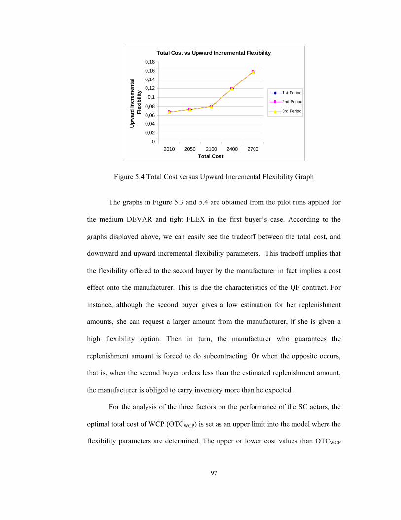
97

Total Cost vs Upward Incremental Flexibility

0

0,02

0,04

0,06

0,08

0,1

0,12

0,14

0,16

0,18

2010 2050 2100 2400 2700Total Cost

Upw

ard

Incr

emen

tal

Flex

ibili

ty 1st Period

2nd Period

3rd Period

Figure 5.4 Total Cost versus Upward Incremental Flexibility Graph

The graphs in Figure 5.3 and 5.4 are obtained from the pilot runs applied for

the medium DEVAR and tight FLEX in the first buyer’s case. According to the

graphs displayed above, we can easily see the tradeoff between the total cost, and

downward and upward incremental flexibility parameters. This tradeoff implies that

the flexibility offered to the second buyer by the manufacturer in fact implies a cost

effect onto the manufacturer. This is due the characteristics of the QF contract. For

instance, although the second buyer gives a low estimation for her replenishment

amounts, she can request a larger amount from the manufacturer, if she is given a

high flexibility option. Then in turn, the manufacturer who guarantees the

replenishment amount is forced to do subcontracting. Or when the opposite occurs,

that is, when the second buyer orders less than the estimated replenishment amount,

the manufacturer is obliged to carry inventory more than he expected.

For the analysis of the three factors on the performance of the SC actors, the

optimal total cost of WCP (OTCWCP) is set as an upper limit into the model where the

flexibility parameters are determined. The upper or lower cost values than OTCWCP

98

are not included, since the optimal WCP cost is the critical cost level, where the

largest replenishment amounts possible are included to the initial model.

The tight and loose flexibilities of the manufacturer for both buyers for

DEVAR set at medium level can be seen in Table 5.9.

Table 5.9 Flexibility Parameters of the Manufacturer at medium DEVAR level and in

different FLEX levels in the Second Case

FLEXIBILITY TIGHTNESS [MEDIUM DEVAR] MANUFACTURER DETERMINES THE CONTRACT PARAMETERS for FIRST BUYER for SECOND BUYER tight loose tight loose ωm1 αm1 ωm1 αm1 ωm2 αm2 ωm2 αm2

1 0.1 0.1 0.2 0.2 0.068 0.068 0.093 0.093 2 0.11 0.11 0.21 0.21 0.068 0.068 0.093 0.093

Perio

d

3 0.12 0.11 0.22 0.22 0.068 0.068 0.093 0.093 , where ωm1 = [ωm1

1, ωm12, ωm1

3], and αm1 = [αm11, αm1

2, αm13]; and ωm2 = [ωm2

1, ωm22,

ωm23], and αm2 = [αm2

1, αm22, αm2

3].

Then, the tight and loose flexibility parameters of the second buyer offered by

the manufacturer, at medium DEVAR level, are as in Table5.10.

Table 5.10 Flexibility Parameters of the Second Buyer at medium DEVAR level in

the Second Case

FLEXIBILITY TIGHTNESS [MEDIUM DEVAR] tight loose ω2 α2 ω2 α2

1 0.016 0.019 0.043 0.043 2 0.016 0.020 0.042 0.044

Perio

d

3 0.015 0.020 0.041 0.044 , where ω2 = [ω2

1, ω22, ω2

3], and α2 = [α21, α2

2, α23].

Since the loose flexibility option is provided to the manufacturer by

increasing the upper total cost limit, these incremental flexibility values are

99

determined by dividing the flexibility parameters of the manufacturer for the second

buyer by RT.

The tight and loose flexibility parameters of the manufacturer for DEVAR

factor at the high level are presented in Table 5.11.

Table 5.11 Flexibility Parameters of the Manufacturer at high DEVAR level and in

different FLEX levels in the Second Case

FLEXIBILITY TIGHTNESS [HIGH DEVAR] MANUFACTURER DETERMINES THE CONTRACT PARAMETERS for FIRST BUYER for SECOND BUYER tight loose tight loose ωm1 αm1 ωm1 αm1 ωm2 αm2 ωm2 αm2

1 0.1 0.1 0.2 0.2 0.117 0.117 0.139 0.139 2 0.11 0.11 0.21 0.21 0.117 0.117 0.14 0.139

Perio

d

3 0.12 0.11 0.22 0.22 0.128 0.117 0.139 0.139 , where ωm1 = [ωm1

1, ωm12, ωm1

3], and αm1 = [αm11, αm1

2, αm13]; and ωm2 = [ωm2

1, ωm22,

ωm23], and αm2 = [αm2

1, αm22, αm2

3].

Then, the tight and loose flexibility parameters of the second buyer offered by

the manufacturer at high DEVAR level are as in Table 5.12.

Table 5.12 Flexibility Parameters of the Second Buyer at high DEVAR level in the

Second Case

FLEXIBILITY TIGHTNESS [HIGH DEVAR] tight loose ω2 α2 ω2 α2

1 0.068 0.066 0.091 0.087 2 0.067 0.067 0.092 0.088

Perio

d

3 0.078 0.067 0.090 0.088 , where ω2 = [ω2

1, ω22, ω2

3], and α2 = [α21, α2

2, α23].

100

COST

For the final factor, cost, the levels are determined such that the cost burden

on each party can be easily controlled. Since SC actors exist in the same

environment; we assume they have the identical inventory carrying costs. As

described in the previous section, the inventory costs of the buyers and the

manufacturer are taken as the base, and all the other costs are determined

accordingly. We also assume that cost values do not differ from period to period. The

unit costs for the buyers and the manufacturer can be seen in Table 5.13.

Table 5.13 Unit Costs of the Supply Chain Actors

COST ($) Low High

inventory holding cost 1 1 backordering cost 3 8

subcontracting cost 2 4 immediate subcontracting cost 4 8

According to the cost values presented in the table above, the tradeoff on the

manufacturer’s side arises in the backordering and subcontracting costs. The low cost

values create no burden on any parties. However, by high backordering cost, the

buyers are forced to carry more inventory in order not to experience shortage.

However, this often results in requesting more from the manufacturer. Thus, the

manufacturer who has a limited capacity is then forced to do more subcontracting, so

has a high cost. Hence, the cost burden is given onto the buyer directly, and also onto

the manufacturer indirectly. In the other case, in which the subcontracting cost is

high, the manufacturer tries to do less subcontracting which is in relation with the

replenishment amounts requested by the buyers, thus, by increasing the

101

subcontracting cost, the burden is given onto the manufacturer. Lastly, when the

costs of the SC parties are all high, the burden is given on all. That is, both buyers try

to make less backordering and the manufacturer tries to do less subcontracting, hence

the objectives are in severe conflict.

5.2.2 GENERATION OF DEMAND DATA

Since the market demand is stochastic, to introduce random market demand

into the problem, a scenario based approach is utilized. The details of the scenario

based approach are introduced in Chapter 3. For the scenario based approach, we

generate discrete alternative values for each period except the current period at the

beginning. The approach for data generation is based on the coefficient of variation

(CV) of the data.

At the beginning of the planning horizon, it is assumed that the buyers have

forecasts performed in the previous period. They are initially assumed given to the

problem and they are taken as the mean of the demand of the related period. The

market demand the buyers face over the horizon is not stationary. We assume they

have some demand information about the market demands through all periods. They

have an increasing coefficient of variation as going away from the current period,

corresponding to an increasing forecast error. However, as time passes, the forecasts

for the demand of the periods are modified by the buyers, forecast CV values

gradually decrease. That is, getting closer to the current period, less uncertainty is

encountered. Therefore, for consistency of treatment, the CV of the period (t+j)

changes to the CV of period (t+j-1) after the calendar moves one period ahead.

102

According to the scenario tree introduced in chapter 3, the data for the first

period, is a single value, since it is the realized market demand for the current period.

The buyer has complete and accurate information for the current period alone. For

the next, second and third periods, 4 possible demand occurrences are generated in

each. Therefore, 43=64 scenarios are constructed. Each has its own chance to be

realized.

For the generation of the data, the CV and the mean values are taken into

account. The approach taken in the demand data generation is finding 4 discrete

values that give the desired CV and mean, where the former represents the forecast

error and the latter, the forecast of the SC actor for all periods except the current

period.

An example of the scenario tree generated for the first buyer can be seen in

Figure 5.5.

Figure 5.5 Scenario Tree generated for the First Buyer

On the first level of the scenario tree in the above figure, there is an exact

value which is the realized market demand. At the second level, i.e., second period,

500

Discrete Demand Values 605 495 575 510

0.3 0.1 0.2 0.4

660 540 520 635

0.3 0.2 0.1 0.4

615 485 585 500

0.3 0.1 0.2 0.4

Probabilities

Period (t+1)

Current Period t

Period (t+3)

Period (t+2)

Mean: 550 and CV: 0.08

Mean: 550 and CV: 0.10

Mean: 600 and CV: 0.09

0.027 0.002 0.004 0.064 Scenario Probabilities

103

and other levels as well, the mean represents the forecast of the buyer for that period.

The discrete values are the random alternative demand occurrences along with their

associated probabilities. The coefficient of variation at a level represents the variance

of the discrete values at that level.

As one period passes, we go down on the scenario tree, another level is

appended to the bottom, and the first level is omitted. This time the second period

becomes the current period; the third period becomes the period just following the

current period. The third and later periods now have different discrete values from

the first scenario tree. They have different (lower) CV, since they become closer to

the current period. However, they are assumed to have the same mean and the same

probabilities. This is because probabilities refer to scenarios (i.e., P(sci)=pi) and are

independent of time. The demand data generated for the first and second buyers at

particular demand variation levels are presented in Appendix A.

As in the buyer’s case, it is also assumed that the forecasts made by the

manufacturer in the previous period are supplied to the problem initially. The

manufacturer forecasts the actual replenishments of the buyers with an increasing CV

getting apart from the current period as well. To be consistent between the SC actors,

the manufacturer and the buyers are assumed to have their initial forecasts identical

to each other. Though the means of their forecasts are assumed to be the same for the

periods, the discrete values, and the associated probabilities to these discrete values

are different for the buyers and the manufacturer. Moreover, it is assumed that the

manufacturer also modifies his forecasts about the actual replenishments of the

buyers as time passes.

104

The manufacturer is subject to two independent scenario trees each related to

a different buyer’s replenishment amounts. On the first levels of the scenario trees,

there are two exact values representing each buyer’s realized actual replenishment

amount. Since the manufacturer encounters two separate scenario trees for each

buyer in the decisions of inventory carrying, production, capacity usage and

subcontracting, he takes all combinations of the two 64 scenarios, thus he is subject

to 64x64 cases in total. The demand data generated for the manufacturer at particular

demand variation levels are presented in Appendix B.

We analyze the manufacturer’s incentives in allocating his limited capacity

and in his subcontracting decisions in a QF environment. The purpose is to examine

at what amount the manufacturer uses his limited capacity, at what amount he gives

orders to the subcontractor and in which situations he determines to subcontract. In

order to determine the fixed capacity limit, we try to cover a large percentage of the

total demands of the buyers. We select this percentage as 80%. The maximum of the

sums of the demand estimations for each period made by each buyer is selected for

calculation. According to the demand data generated for both buyers, the

manufacturer’s capacity is determined as 1000 units covering at least 80% of the

maximum estimated total demand.

5.3 STATISTICAL ANALYSIS

In order to analyze the attitudes of the SC actors and their benefits gathered

both in the individual and in the integrated supply chain environment, we conduct a

statistical analysis on the performance measures determined. We try whether the

105

performance measures obtained are significantly different for different levels of the

three factors, DEVAR, FLEX, and COST.

We first determine the required sample size for the statistical analysis. For the

first and second buyers, there are 64 scenarios having different probabilities of

occurrence. In order to make our analysis on the performance measures determined

for the SC actors, we determined the required sample size to construct a 90%

confidence interval (CI) for the 64 scenarios. Since all periods in the planning

horizon are independent from each other, we independently calculate the sample size

for each period considering the mean and variation of that period’s demand.

According to the determined sample size for each period, the maximum sample size

among all periods is obtained. Then, utilizing the Random Data Generation option of

the statistical software MINITAB, we take a specified number of samples from 64

scenarios and make our analysis using these samples.

For the manufacturer, the randomness stem from the actual replenishment

amounts of the two buyers. Therefore, in order to determine the required sample size,

pilot runs are carried out. Same as the buyers’ cases, the periods in the planning

horizon are independent from each other. The required sample size is calculated for

the first and the second buyer’s replenishment amounts individually. The

manufacturer is subject to the combination of both buyers’ replenishment amounts,

where they are also independent from each buyer’s. Thus, the summation of the

means and variations of first and second buyers for each period is also calculated to

determine the sample size. The maximum among these three calculated sample sizes

is taken to generate samples from the combination of 64 scenarios for each buyer,

106

that is, from 64x64 scenarios. The samples generated for each SC actor is given in

Appendix C.

The required sample size for the integrated supply chain is determined with

the same approach utilized in the calculations of the manufacturer’s required sample

size.

5.4 GAMS MODEL

In order to solve the two-stage stochastic models constructed, the

optimization software General Algebraic Modeling (GAMS) is run. This

optimization software has many advantages that encourage us its use. It provides a

high-level language for the compact representation of large and complex models,

allows changes to be made in model specification simply and safely, permits model

descriptions that are independent of solution algorithms, and finally solves more than

one model in a single run.

Since our model gets larger as the number of scenarios gets larger, the

GAMS/Cplex solver is selected. GAMS/Cplex allows for combining the high level

modeling capabilities of GAMS with the power of Cplex optimizers. While

numerous solving options are available, GAMS/Cplex automatically calculates and

sets most options at the best values for specific problems.

Moreover, for the initial models in the case where the second buyer

determines her flexibility parameters, and the case where the manufacturer

determines the flexibility parameters to be offered to the second buyer, a non-linear

programming model is solved. For the non-linear model, MINOS, which is a general

107

purpose nonlinear programming solver is utilized. GAMS/MINOS is designed to find

solutions that are locally optimal.

In the application of the Benders Decomposition Algorithm, there is a loop,

where sub and master problems are iteratively solved. One single GAMS model is

comprised of three models, which are the Worst Case Problem (WCP), the sub

problem and the master problem. Initially, the WCP is solved. The solutions are

introduced to the sub problem. By the LOOP option in GAMS, we construct a loop

where the sub problem is solved first. The solutions of the sub problem at each

iteration are saved in specified parameters, and are introduced to the master problem

as numerical values. Thus, at each iteration one constraint is added to the master

problem. Afterwards, the master problem is solved. Then the new master problem

solutions are included into the sub problem as numerical values, and new sub

problem is solved. When the terminating condition, which is written again at the

beginning of the loop, is satisfied, the loop terminates. Thus, by the LOOP option,

the two-stage stochastic programming models constructed are solved in a single run.

An example for the two-stage stochastic model of the first buyer applied in

GAMS is presented in Appendix D.

108

CHAPTER VI

ANALYSIS

In this study, we analyze the attitudes of SC actors in a specified environment

and their incentives in their medium and short term decisions. The environmental

characteristics are comprised of who determines the contract flexibility parameters,

how the values of the flexibility parameters are decided, the tightness of the

flexibilities, the variability of the demand the SC actors face, and the costs associated

with their medium and short term decisions.

Given the different factors levels explained in the previous chapter, and the

decision making situations of the flexibility parameters for the second buyer, a full

factorial experiment is performed. The objective of this experiment is to investigate

the individual and system wide behaviors of the SC actors in different cases and

under the effects of the environmental characteristics.

In this chapter, the effects of the factor levels on the average cost of each SC

actor are analyzed statically utilizing the SAS (Statistical Analysis System) software.

In $6.1, some initial observations related with the attitudes in the determination of

the flexibility parameters and the character of typical sample runs, are presented. In

$6.2, the approaches taken in modeling to compare different factors are stated. In

$6.3, the outcomes of the full factorial experiment and the underlying reasoning

behind these particular behaviors are proposed. Moreover, a statistical analysis to

109

compare whether there is a significant difference between individual and coordinated

activity is performed.

6.1 INITIAL OBSERVATIONS

Before analyzing the system in detail, we want to give some initial

observations about the behavior of the SC actors in a given sample under specific

factor levels.

In both cases, where the decision maker (DM) of the flexibility parameters to

be applied to the second buyer differs, the DM’s try to realize relatively higher

flexibility parameter values as the DEVAR gets higher. This implies that as DEVAR

gets higher, the willingness to use the flexibility options provided by the QF

contracts and to pay the price for the option increases.

Although the constant capacity limit is set to cover at least 80% of the

maximum total demand forecasts over the two buyers, the order amount given to the

subcontractor is higher than 20%, which indicates that the manufacturer does not use

his capacity in full. The reason for this is that the manufacturer opts to carry

inventory into the future periods. Since he does not know the intended future

replenishment amounts of the buyers by certainty, he makes his plans according to

his forecasts. Thus, he tries to cover all possible forecasted replenishment values, and

often gives larger than possibly needed orders to the subcontractor.

The manufacturer’s average cost increases in the second case where he

determines the flexibility parameters with respect to the one in the first case. This is

due to the replenishment amounts requested by the second buyer. Since she

110

determines the parameters herself in the first case, she makes contract obligations

more efficient, that is, more effective bounds are constructed so that her estimates

can fall within them. Thus, she can request less when a lower demand occurs, which

in fact affects the cost of the manufacturer in a positive way.

We are also interested in the information sharing and control scheme of the

SC actors, that is, their environments. The decisions of the buyers and the

manufacturer in the individual and the integrated supply chain environments under

identical realized demand quantities are presented below. The purpose is to display

the change in the estimated replenishment amounts as time passes, and the changes

in the decisions where all actors are involved in a single game. First, we present

Table 6.1 and 6.2 for the SC actors to display their decisions through the passage of

time for four periods.

Table 6.1 Notations of the First Buyer’s Decisions on a Rolling Horizon

FIRST BUYER

t=1 µ01(1) t=2 µ01(2) t=3 µ01(3) t=4 µ01(4) Before After Before After Before After Before After inv1(0) inv1(1) inv1(1) inv1(2) inv1(2) inv1(3) inv1(3) inv1(4)

back1(0) back1(1) back1(1) back1(2) back1(2) back1(3) back1(3) back1(4)

f11(0) f01(1)

f21(0) f11(1) f11(1) f01(2)

f31(0) f21(1) f21(1) f11(2) f11(2) f01(3)

f31(1) f31(1) f21(2) f21(2) f11(3) f11(3) f01(4)

f01(2) f31(2) f31(2) f21(3) f21(3) f11(4)

f01(3) f01(3) f31(3) f31(3) f21(4)

f01(4) f01(4) f01(4) f31(4)

f01(5) f01(5) f01(5)

f01(6) f01(6)

f01(7)

111

Every period is depicted in two columns, denoted by “before” and “after”.

The former shows input data coming from the end of the previous period which is

utilized in the current period. The latter shows the decisions of the current period and

the input data to be exploited in the next period. The decisions of not only the

estimated replenishments in period t, )(tbf j ’s, but also the inventory carrying or

backordering as of end of period t, )(tinvb and )(tbackb are transferred to the next

period (t+1) as input. The )(tbf j ’s are also conveyed to the manufacturer.

The )(0 tbf ’s are the actual replenishment amounts decided according to the realized

demand, )(0 tbµ ’s. The )(0 jtbf + ’s are the intended future replenishment amounts,

which are in fact the internal plans and which will be the actual replenishment

amount as period (t+j) becomes the current period. As seen from the table above,

there is a dynamics through all periods. For instance, the estimate for the third period

made initially, )0(13f changes to the estimate made in the first period )1(12f , then to

the estimate made in the second period )2(11f , and eventually the actual

replenishment amount requested in the third period )3(10f .

112

Table 6.2 Notations of the Manufacturer’s Decisions on a Rolling Horizon

MANUFACTURER For First Buyer

t=1 f01(1) t=2 f01(2) t=3 f01(3) t=4 f01(4) Before After Before After Before After Before After

invmp1(0) subexp1 invmp1(1) subexp1 invmp1(2) subexp1 invmp1(3) subexp1 invm1(1) invm1(2) invm1(3) invm1(4)

r11(0) r01(1)

r21(0) r11(1) r11(1) r01(2)

r31(0) r21(1) r21(1) r11(2) r11(2) r01(3)

r31(1) r31(1) r21(2) r21(2) r11(3) r11(3) r01(4)

r01(2) r31(2) r31(2) r21(3) r21(3) r11(4)

r01(3) r01(3) r31(3) r31(3) r21(4)

r01(4) r01(4) r01(4) r31(4)

r01(5) r01(5) r01(5)

r01(6) r01(6)

For Second Buyer r01(7)

t=1 f02(1) t=2 f02(2) t=3 f02(3) t=4 f02(4) Before After Before After Before After Before After

invmp2(0) subexp2 invmp2(1) subexp2 invmp2(2) subexp2 invmp2(3) subexp2 invm2(1) invm2(2) invm2(3) invm2(4)

r12(0) r02(1)

r22(0) r12(1) r12(1) r02(2)

r32(0) r22(1) r22(1) r12(2) r12(2) r02(3)

r32(1) r32(1) r22(2) r22(2) r12(3) r12(3) r02(4)

r02(2) r32(2) r32(2) r22(3) r22(3) r12(4)

r02(3) r02(3) r32(3) r32(3) r22(4)

r02(4) r02(4) r02(4) r32(4)

r02(5) r02(5) r02(5)

r02(6) r02(6)

r02(7) sub(2) sub(3) sub(4) sub(5)

The table above is similar to the buyer’s tables. It is composed of two

separate tables one for the first and one for the second buyer. The )(10 tf , as can be

followed in Table 6.1 and )(20 tf ’s are the realized replenishment amounts of the first

113

and second buyers in period t, respectively. The manufacturer has release schedules

specific for each buyer. The decisions of not only the estimated releases in period

t, )(tbrj ’s, but also the subcontracting, )1( +tsub ’s, are conveyed to the next period

(t+1) as in the buyers’ cases. )(exp tbsub ’s are the immediate subcontracting

decisions not transferred to the next period. )(tinvmb ’s are the resultant inventory in

period t, and )(tinvmpb ’s are the inventory taken from the total pooled inventory in

period t which will be used in period (t+1) (i.e., )(1 tinvm and )(2 tinvm can be

realloacted). )(0 jtbr + ’s are the intended future release amounts that can be modified

on a rolling horizon basis. )1( +tsub ’s refer to the order given to the subcontractor in

period t to be received in period (t+1).

The example is given for the case where the second buyer determines the

flexibility parameters. The DEVAR level is high, and the FLEX level of both the

first buyer and the manufacturer are tight. In the sample, the demand realizations for

the first buyer are 500, 600, 720, and 440 units for the first, second, third, and fourth

periods, respectively. The actual and estimated replenishment, inventory carrying

and backordering decisions taken in the individual environment of the first buyer are

presented in Table 6.3.

114

Table 6.3 Decisions of the First Buyer in her Individual (Decentralized) Environment

FIRST BUYER INDIVIDUAL ENVIRONMENT

t=1 µ01(1)=500 t=2 µ01(2)=600 t=3 µ01(3)=720 t=4 µ01(4)=440 Before After Before After Before After Before After

inv1(0)=0 inv1(1)=0 inv1(1)=0 inv1(2)=0 inv1(2)=0 inv1(3)=0 inv1(3)=0 inv1(4)=151.7back1(0)=0 back1(1)=0 back1(1)=0 back1(2)=0 back1(2)=0 back1(3)=5.5 back1(3)=5.5 back1(4)=0

500.0 500

550.0 583.0 583.0 600

660.0 642.0 642.0 680.5 680.5 714.5

577.9 577.9 593.0 593.0 628.6 628.6 597.1

604.5 604.5 646.9 646.9 608.0

554.2 554.2 579.7

503.8

Since the estimated replenishment amount for the third period determined in

the second period is low (680.5 relative to the realized demand 720), the first buyer

unavoidably backorders some part of the third period’s demand. However, due to the

backordering, she determines the estimated replenishments to be utilized in the next

period, with higher values. However, in the fourth period, she realizes a low demand

again, and ends up with inventory. She, in turn, lowers her estimated replenishment

amounts, as seen in the table above. For instance, the value of )2(13f , i.e., 604.5

units, which refers to the fifth period’s estimate in the second period happens to be

enlarged to 646.9 units in third period, and in the fourth period, the estimate, )4(11f

takes the lower value of 608 units. For the intended future replenishment amounts, no

numerical values are included, since the internal plans are determined subject to each

64 scenario. This situation for the intended future replenishment and release amounts

is also valid for the other SC actors.

115

The decisions of the second buyer in a sample are included in Table 6.4.

Table 6.4 Decisions of the Second Buyer in her Individual Environment

SECOND BUYER INDIVIDUAL ENVIRONMENT

t=1 µ02(1)=550 t=2 µ02(2)=650 t=3 µ02(3)=740 t=4 µ02(4)=720 Before After Before After Before After Before After

inv2(0)=0 inv2(1)=0 inv2(1)=0 inv2(2)=0 inv2(1)=0 inv2(2)=0 inv2(1)=0 inv2(2)=0 back2(0)=0 back2(1)=0 back2(1)=0 back2(2)=0 back2(1)=0 back2(2)=0 back2(1)=0 back2(2)=0.1

550.0 550

600.0 600.0 600.0 650

650.0 650.0 650.0 650.0 650.0 740

307.8 307.8 321.4 321.4 321.4 321.4 719.9

342.0 342.0 357.1 357.1 357.1

307.8 307.8 321.4

282.2

Since her downward incremental flexibilities, jω ’s, for all periods and the

upward, jα ’s for the second period are zero, the estimated replenishment amount of

period (t+2) can not be modified as time passes. As seen from the table above, the

value of )1(12f , i.e., the estimate for the third period made in the first period, is 650

units, which does not change as time passes. The value of )2(11f , i.e., the estimate in

the second period, is again 650 units.

The replenishment amounts determined by the two buyers are requested from

the manufacturer. The manufacturer being ordered the realized replenishment

amounts makes the following set of decisions presented in Table 6.5.

116

Table 6.5 Decisions of the Manufacturer in his Individual Environment

MANUFACTURER INDIVIDUAL ENVIRONMENT For First Buyer

t=1 f01(1)=500 t=2 f01(2)=600 t=3 f01(3)=714.5 t=4 f01(4)=597.1Before After Before After Before After Before After

invmp1(0)=0 subexp1=22.5 invmp1(1)=0 subexp1=0 invmp1(2)=130 subexp1=0 invmp1(3)=13 subexp1=0

invm1(1)=0 invm1(2)=0 invm1(3)=0 invm1(4)=30.6

500.0 477.5

550.0 600.0 600.0 600.0

600.0 589.7 589.7 536.6 536.6 584.5

482.5 482.5 540.4 540.4 599.8 599.8 614.7

526.3 526.3 589.5 589.5 654.3

482.5 482.5 540.4

For Second Buyer 453.2

t=1 f02(1)=550 t=2 f02(2)=650 t=3 f02(3)=740 t=4 f02(4)=719.9

Before After Before After Before After Before After

invmp2(0)=0 subexp2=27.5 invmp2(1)=0 subexp2=0 invmp2(2)=0 subexp2=0 invmp2(3)=32.7 subexp2=0

invm2(1)=0 invm2(2)=130 invm2(3)=45.7 invm2(4)=32.7

500.0 522.5

550.0 570.0 570.0 780.0

600.0 617.5 617.5 586.6 586.6 785.7

267.7 267.7 291.7 291.7 306.3 306.3 719.9

290.0 290.0 316.0 316.0 331.8

267.7 267.7 291.7

245.4

sub(2)=380 sub(3)=370.2 sub(4)=334.6 sub(5)=437

It is observed that all realized replenishment amounts are satisfied by that

period’s release amounts and by the subcontracting and the inventory carried from

the previous period, except the first period. The manufacturer is forced to

immediately subcontract 22.5 and 27.5 units for the first and second buyer,

respectively in the first period due to the insufficient capacity. The large

subcontracting amounts can be easily detected. These large amounts are not only due

to the limited capacity of the manufacturer. They are also built up in trying to carry

117

inventory for the future periods. Since he doesn’t know the intended future

replenishment amounts of the buyers, he makes his plans according to his own

forecasts. For instance, in the first period, his forecasts for the first buyer are 660,

440, 480, and 595 units for the second period. However, the first buyer’s intended

future replenishment amounts determined in the first period are 612.5, 553.85, and

600 units over all scenarios. Due to the obligation to release the requested

replenishment amounts to be requested later, he tries to make his subcontracting

decision covering all possible forecasted replenishments which are often larger than

the internal self plans of the buyers.

The three tables, (Table 6.3-5), above are defined by the three SC actors’

acting individually. Now three tables for the SC actors will be presented when they

play the same supply chain game in a coordinated manner, with demand realizations

for the two buyers held identical. The intuition is that, in this specific environment,

the decisions of the first buyer and the manufacturer differ when the medium and

short term decisions of each SC actor are accurately informed to each other.

Table 6.6 Decisions of the First Buyer in the Integrated Supply Chain

(Centralized) Environment

FIRST BUYER

INTEGRATED SUPPLY CHAIN ENVIRONMENT

t=1 µ01(1)=500 t=2 µ01(2)=600 t=3 µ01(3)=720 t=4 µ01(4)=440 Before After Before After Before After Before After

inv1(0)=0 inv1(1)=0 inv1(1)=0 inv1(2)=0 inv1(2)=0 inv1(3)=0 inv1(3)=0 inv1(4)=87.1 back1(0)=0 back1(1)=0 back1(1)=0 back1(2)=0 back1(2)=0 back1(3)=70 back1(3)=70 back1(4)=0

500.0 500

550.0 583.0 583.0 600

660.0 642.0 642.0 619.0 619.0 650

577.9 577.9 593.0 593.0 628.6 628.6 597.1

604.5 604.5 646.7 646.7 607.9

581.8 581.8 593.0

503.8

118

Table 6.7 Decisions of the Second Buyer in the Integrated Supply Chain Environment

SECOND BUYER

INTEGRATED SUPPLY CHAIN ENVIRONMENT

t=1 µ02(1)=550 t=2 µ02(2)=650 t=3 µ02(3)=740 t=4 µ02(4)=720 Before After Before After Before After Before After

inv2(0)=0 inv2(1)=0 inv2(1)=0 inv2(2)=0 inv2(1)=0 inv2(2)=0 inv2(1)=0 inv2(2)=0 back2(0)=0 back2(1)=0 back2(1)=0 back2(2)=0 back2(1)=0 back2(2)=0 back2(1)=0 back2(2)=0.1

550.0 550

600.0 600.0 600.0 650

650.0 650.0 650.0 650.0 650.0 740

307.8 307.8 321.4 321.4 321.4 321.4 719.9

342.0 342.0 357.1 357.1 357.1

307.9 307.9 321.4

282.2

119

Table 6.8 Decisions of the Manufacturer in the Integrated Supply Chain Environment

MANUFACTURER

INTEGRATED SUPPLY CHAIN ENVIRONMENT

For First Buyer

t=1 f01(1)=500 t=2 f01(2)=600 t=3 f01(3)=650 t=4 f01(4)=597.1Before After Before After Before After Before After

invmp1(0)=0 subexp1=22.5 invmp1(1)=0 subexp1=0 invmp1(2)=12.2 subexp1=0 invmp1(3)=0 subexp1=0

invm1(1)=0 invm1(2)=0 invm1(3)=0 invm1(4)=61.5

500.0 477.5

550.0 610.5 610.5 600.0

600.0 643.0 643.0 579.9 579.9 637.8

503.1 503.1 563.5 563.5 600.0 600.0 658.6

526.3 526.3 589.5 589.5 524.6

506.5 506.5 567.3

For Second Buyer 438.6

t=1 f02(1)=550 t=2 f02(2)=650 t=3 f02(3)=740 t=4 f02(4)=719.9

Before After Before After Before After Before After

invmp2(0)=0 subexp2=27.5 invmp2(1)=0 subexp2=0 invmp2(2)=0 subexp2=0 invmp2(3)=0 subexp2=68.6

invm2(1)=0 invm2(2)=12.2 invm2(3)=0 invm2(4)=0

500.0 522.5

550.0 570.0 570.0 662.2

600.0 617.5 617.5 586.6 586.6 740.0

267.7 267.7 291.7 291.7 277.2 277.2 651.3

297.4 297.4 324.1 324.1 313.5

267.7 267.7 291.7

245.4

sub(2)=262.2 sub(3)=377.8 sub(4)=309.9 sub(5)=256.1

The manufacturer now sees the intended future replenishment decisions. He

determines the amount of inventory carried and order to be given to the subcontractor

based on these intended future plans. It can easily be observed that the amount of

inventory carried and order given to the subcontractor definitely decrease in the

integrated supply chain, (i.e., in the centralized environment). For instance,

the )2(sub , )4(sub and )5(sub values decrease from 380, 334.6, and 437 units to

262.2, 309.9, and 256.1 units, respectively. Also, the inventory of 130 units carried

120

from the second period to the third period decreases to 12.2 units in the integrated

supply chain solution. However, in the integrated SC, the manufacturer is forced to

use the immediate subcontracting option in the fourth period, whereas he doesn’t

order to the subcontractor in his individual environment.

The first buyer in turn does not get into a better position when he is involved

into the integrated supply chain. She only backorders 5.5 units in her individual

environment, whereas in the integrated SC, she backorders 70 units, which indeed

yields high cost for her. But, the inventory carried in the fourth period of the first

buyer decreases from 151.7 to 87.1 units.

Finally, for this particular sample, only the manufacturer favors to be

involved in the integrated supply chain. The first buyer is willing to behave

individually, because in order to make the systemwide performance better, the cost

burden due to the subcontracting is put onto her. As a result of the information

shared, the estimated replenishment and release amounts also change to a certain

extent. However, the second buyer’s estimates and decisions of inventory carrying

and backordering do not change, indicating that the cost substitution occurs between

the first buyer and the manufacturer. Being the DM of her flexibility parameters, i.e.,

figuring some part of the environmental characteristics, she gets the advantage of the

flexibility parameters in her offered QF contract.

6.2. STATISTICAL EXPERIMENTATION MODELS

In order to analyze the consequences of the factor levels on the accrued costs

of the SC actors, we construct different statistical models. The difference is sought

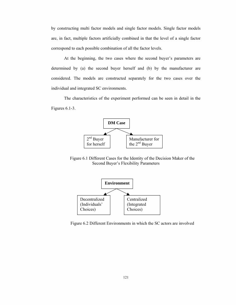
121

by constructing multi factor models and single factor models. Single factor models

are, in fact, multiple factors artificially combined in that the level of a single factor

correspond to each possible combination of all the factor levels.

At the beginning, the two cases where the second buyer’s parameters are

determined by (a) the second buyer herself and (b) by the manufacturer are

considered. The models are constructed separately for the two cases over the

individual and integrated SC environments.

The characteristics of the experiment performed can be seen in detail in the

Figures 6.1-3.

Figure 6.1 Different Cases for the Identity of the Decision Maker of the Second Buyer’s Flexibility Parameters

Figure 6.2 Different Environments in which the SC actors are involved

DM Case

2nd Buyer for herself

Manufacturer for the 2nd Buyer

Environment

Decentralized (Individuals’ Choices)

Centralized (Integrated Choices)

122

Figure 6.3 Different Levels of DEVAR, FLEX and COST Factors

As seen in Figure 6.3, the DEVAR factor is systemwide, whereas the FLEX

and COST factors are dependent on the SC actors. In the first case, the tight and

loose FLEX levels of the first buyer implies the incremental flexibility parameters

that are utilized by her, and are in relation with the manufacturer with the cumulative

flexibility parameters, which are in fact multiples of the incremental ones. The

manufacturer in turn has tight and loose FLEX levels for each buyer, which are used

for his own plans. In the second case, the tight and loose FLEX levels of the second

buyer indicates the incremental flexibility parameters offered after the determination

of the tight and loose incremental flexibility parameters of the manufacturer. The

determination processes for both cases are explained in the previous chapter.

Different approaches in designing the models are taken into account. In the

multi factor models, initially, the DEVAR factor is not involved, since it is a

systemwide factor, whereas the others are SC actor dependent. The FLEX and COST

factors are analyzed in different DEVAR levels to see the effects of the two factor

levels in a particular environment. Then, to capture the effect of DEVAR where the

Factor

DEVAR COST FLEX

Medium High Tight Loose Low High

Systemwide (common)

SC Actor dependent (by actor)

123

other factors are assigned differently, models consisting of the three factor levels are

constructed. Thirdly, all combinations of the FLEX and COST factor level are

assigned as levels of a single factor. Finally, the DEVAR factor is also included, and

every viable combination of levels for these three factors is treated as levels of a

single factor. The aim in these last experiments is to see the effect of every

combination of the factors within all possible combinations in the two different

cases.

In the case, where the second buyer determines her own flexibility

parameters, the factor levels to be analyzed differ for the SC actors both in the

individual and in the integrated supply chain environments. Since the first buyer has

loose and tight FLEX levels in her separate environment, a model having only two

factors, FLEX and COST (with two levels for each factor) at different DEVAR

levels is constructed. The model content is presented in Table 6.9.

Table 6.9 Statistical Model Content of the First Buyer in her Individual Environment

DEVAR level FLEXIBILITY TIGHTNESS(FB,FM)

Medium (M) or High (H) tight (T,*) loose (L,*)

low (L,*)

CO

ST(C

B,C

M)

high (H,*)

* represents all different levels of the manufacturer.

In Table 6.9, the notation (FB,FM) and (CB,CM) stands for the FLEX levels of

the buyers and the manufacturer, and COST levels of the buyers and the

manufacturer, respectively.

Since the second buyer determines her flexibility parameters, there are no

loose or tight levels of her FLEX parameter. Hence, a model consisting of only one

124

factor, COST with two levels, low and high is constructed at particular DEVAR

levels for the second buyer.

As for the manufacturer, at a specific DEVAR level, the model has two

factors, FLEX and COST, with four settings each. The four settings of each FLEX

and COST factors are comprised of the combination of the buyers’ and the

manufacturer’s FLEX levels and combination of two parties’ COST levels,

respectively. This is due to the fact that the loose or tight FLEX and low or high

COST levels of the buyers in fact affect the actual replenishment amounts to be

requested from the manufacturer. Since the decisions of inventory carrying,

subcontracting and immediate subcontracting are related to the exact replenishment

amounts, the manufacturer also faces effects of the FLEX and COST levels of the

buyers. Hence, the manufacturer’s model content can be presented in Table 6.10.

Table 6.10 Statistical Model Content of the Manufacturer in his Individual Environment

DEVAR Level FLEXIBILITY TIGHTNESS(FB,FM)

Medium (M) or High (H) (T,T) (T,L) (L,T) (L,L) (L,L) (L,H) (H,L)

CO

ST(C

B,C

M)

(H,H)

For the integrated supply chain, all FLEX and COST levels affect individual

costs of the SC actors. This is true as they act in a coherent system, where all

information about the medium and short term decisions are perfectly shared. For

instance, although the second buyer has no distinction as to loose or tight level of

FLEX, the tight or loose FLEX levels of the first buyer and the manufacturer can

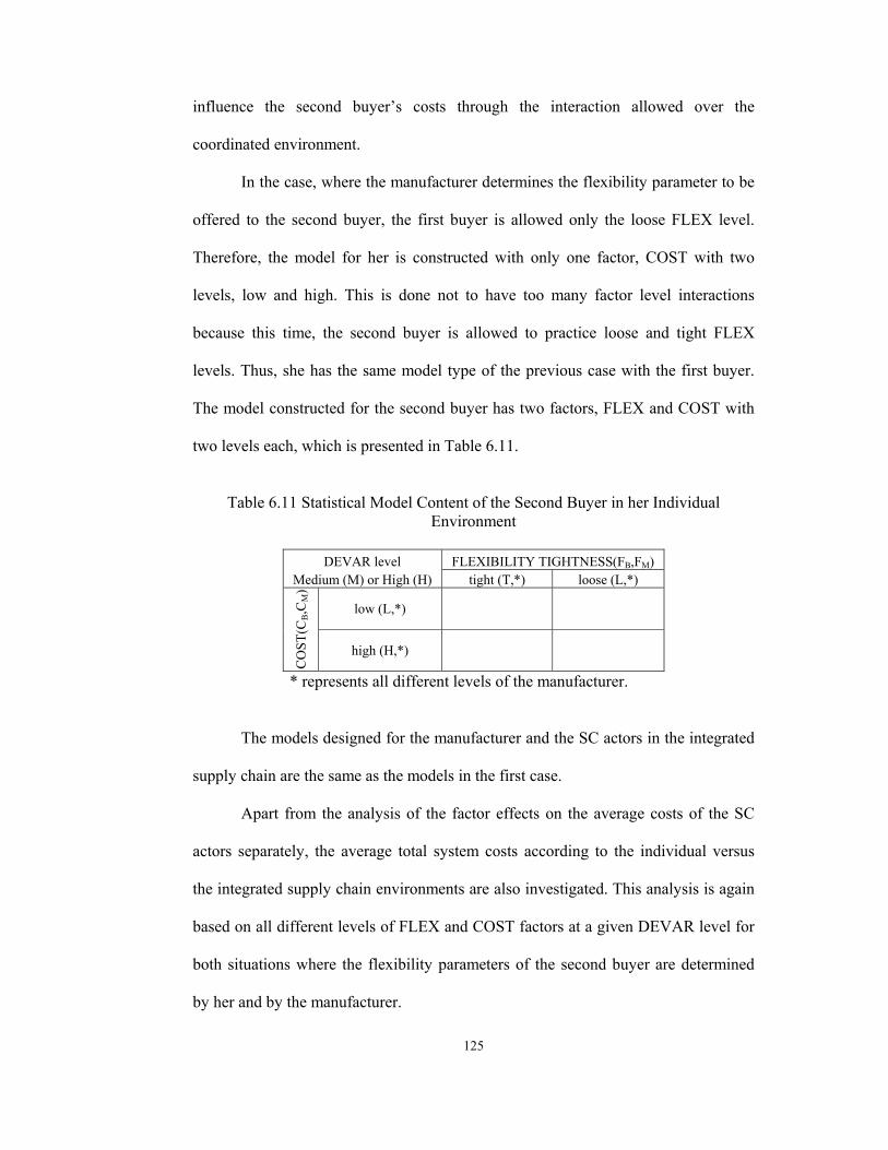
125

influence the second buyer’s costs through the interaction allowed over the

coordinated environment.

In the case, where the manufacturer determines the flexibility parameter to be

offered to the second buyer, the first buyer is allowed only the loose FLEX level.

Therefore, the model for her is constructed with only one factor, COST with two

levels, low and high. This is done not to have too many factor level interactions

because this time, the second buyer is allowed to practice loose and tight FLEX

levels. Thus, she has the same model type of the previous case with the first buyer.

The model constructed for the second buyer has two factors, FLEX and COST with

two levels each, which is presented in Table 6.11.

Table 6.11 Statistical Model Content of the Second Buyer in her Individual

Environment

DEVAR level FLEXIBILITY TIGHTNESS(FB,FM) Medium (M) or High (H) tight (T,*) loose (L,*)

low (L,*)

CO

ST(C

B,C

M)

high (H,*)

* represents all different levels of the manufacturer.

The models designed for the manufacturer and the SC actors in the integrated

supply chain are the same as the models in the first case.

Apart from the analysis of the factor effects on the average costs of the SC

actors separately, the average total system costs according to the individual versus

the integrated supply chain environments are also investigated. This analysis is again

based on all different levels of FLEX and COST factors at a given DEVAR level for

both situations where the flexibility parameters of the second buyer are determined

by her and by the manufacturer.

126

The average costs of the SC actors and the overall system in the decentralized

and centralized environments with respect to different factor levels in the first DM

case are presented in Table 6.12 and Table 6.13 below. The average cost table in

both environments, in the second case can be seen in Appendix E and Appendix F.

Table 6.12 Average Costs of the SC Actors in the Decentralized Environment

DEVAR: Medium/High ; FLEX: Tight/Loose ; COST: Low/High DECENTRALIZED ENVIRONMENT

DEVAR (FB1, FM) / (CB, CM) 1st Buyer 2nd Buyer Manufacturer Total (T,T) / (L,L) 85.9 63.3 2360.0 2509.2 (T,T) / (L,H) 85.9 63.3 4318.7 4467.9 (T,T) / (H,L) 85.9 63.3 2360.1 2509.3 (T,T) / (H,H) 85.9 63.3 4318.9 4468.1 (T,L) / (L,L) 85.9 63.3 2359.2 2508.3 (T,L) / (L,H) 85.9 63.3 4317.4 4466.6 (T,L) / (H,L) 85.9 63.3 2359.2 2508.4 (T,L) / (H,H) 85.9 63.3 4317.6 4466.8 (L,T) / (L,L) 0.0 63.3 2313.4 2376.7 (L,T) / (L,H) 0.0 63.3 4178.8 4242.1 (L,T) / (H,L) 0.2 63.3 2313.6 2377.2 (L,T) / (H,H) 0.2 63.3 4179.5 4243.1 (L,L) / (L,L) 0.0 63.3 2312.5 2375.8 (L,L) / (L,H) 0.0 63.3 4177.5 4240.8 (L,L) / (H,L) 0.2 63.3 2312.7 2376.3

MED

IUM

DEV

AR

(L,L) / (H,H) 0.2 63.3 4178.2 4241.8 (T,T) / (L,L) 290.1 86.8 3211.6 3588.5 (T,T) / (L,H) 290.1 86.8 5913.4 6290.2 (T,T) / (H,L) 370.7 86.8 3302.5 3760.0 (T,T) / (H,H) 370.7 86.8 6095.4 6552.9 (T,L) / (L,L) 290.1 86.8 3210.8 3587.6 (T,L) / (L,H) 290.1 86.8 5912.7 6289.6 (T,L) / (H,L) 370.7 86.8 3306.7 3764.2 (T,L) / (H,H) 370.7 86.8 6084.2 6541.7 (L,T) / (L,L) 130.6 86.8 3144.5 3361.8 (L,T) / (L,H) 130.6 86.8 5711.8 5929.1 (L,T) / (H,L) 130.9 86.8 3144.8 3362.5 (L,T) / (H,H) 130.9 86.8 5712.5 5930.2 (L,L) / (L,L) 130.6 86.8 3143.9 3361.2 (L,L) / (L,H) 130.6 86.8 5710.9 5928.2 (L,L) / (H,L) 130.9 86.8 3144.1 3361.8

HIG

H D

EVA

R

(L,L) / (H,H) 130.9 86.8 5711.5 5929.2

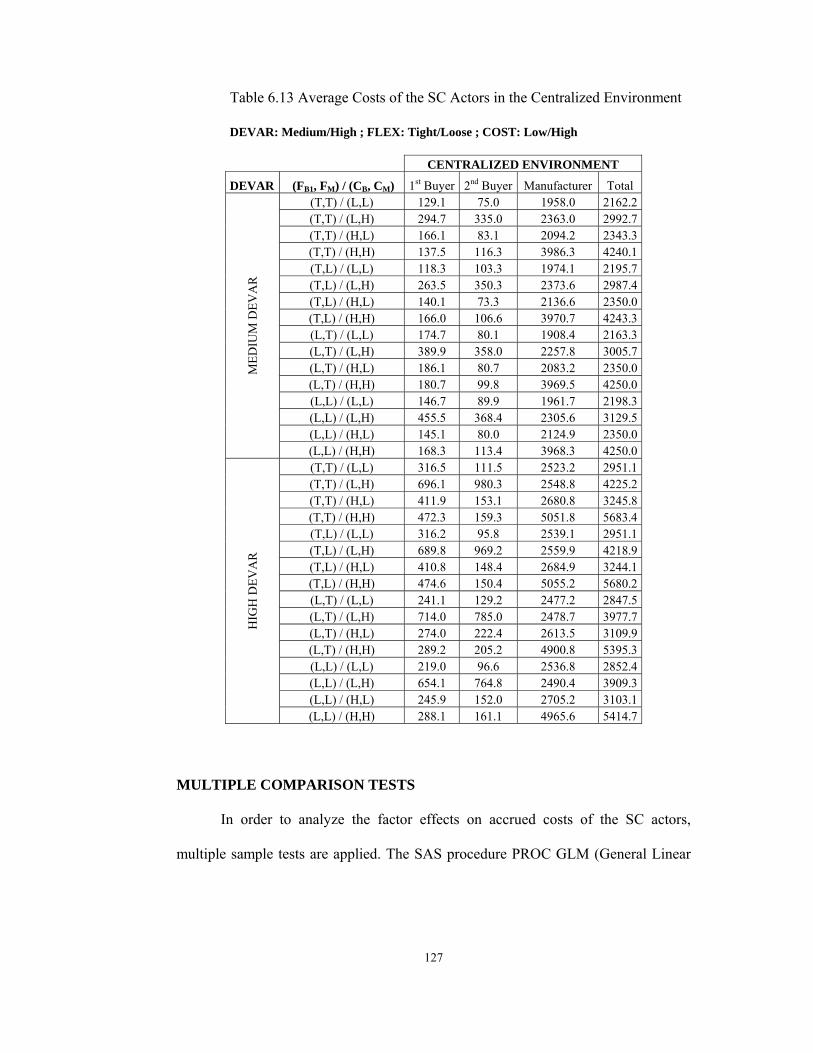
127

Table 6.13 Average Costs of the SC Actors in the Centralized Environment

DEVAR: Medium/High ; FLEX: Tight/Loose ; COST: Low/High CENTRALIZED ENVIRONMENT

DEVAR (FB1, FM) / (CB, CM) 1st Buyer 2nd Buyer Manufacturer Total (T,T) / (L,L) 129.1 75.0 1958.0 2162.2 (T,T) / (L,H) 294.7 335.0 2363.0 2992.7 (T,T) / (H,L) 166.1 83.1 2094.2 2343.3 (T,T) / (H,H) 137.5 116.3 3986.3 4240.1 (T,L) / (L,L) 118.3 103.3 1974.1 2195.7 (T,L) / (L,H) 263.5 350.3 2373.6 2987.4 (T,L) / (H,L) 140.1 73.3 2136.6 2350.0 (T,L) / (H,H) 166.0 106.6 3970.7 4243.3 (L,T) / (L,L) 174.7 80.1 1908.4 2163.3 (L,T) / (L,H) 389.9 358.0 2257.8 3005.7 (L,T) / (H,L) 186.1 80.7 2083.2 2350.0 (L,T) / (H,H) 180.7 99.8 3969.5 4250.0 (L,L) / (L,L) 146.7 89.9 1961.7 2198.3 (L,L) / (L,H) 455.5 368.4 2305.6 3129.5 (L,L) / (H,L) 145.1 80.0 2124.9 2350.0

MED

IUM

DEV

AR

(L,L) / (H,H) 168.3 113.4 3968.3 4250.0 (T,T) / (L,L) 316.5 111.5 2523.2 2951.1 (T,T) / (L,H) 696.1 980.3 2548.8 4225.2 (T,T) / (H,L) 411.9 153.1 2680.8 3245.8 (T,T) / (H,H) 472.3 159.3 5051.8 5683.4 (T,L) / (L,L) 316.2 95.8 2539.1 2951.1 (T,L) / (L,H) 689.8 969.2 2559.9 4218.9 (T,L) / (H,L) 410.8 148.4 2684.9 3244.1 (T,L) / (H,H) 474.6 150.4 5055.2 5680.2 (L,T) / (L,L) 241.1 129.2 2477.2 2847.5 (L,T) / (L,H) 714.0 785.0 2478.7 3977.7 (L,T) / (H,L) 274.0 222.4 2613.5 3109.9 (L,T) / (H,H) 289.2 205.2 4900.8 5395.3 (L,L) / (L,L) 219.0 96.6 2536.8 2852.4 (L,L) / (L,H) 654.1 764.8 2490.4 3909.3 (L,L) / (H,L) 245.9 152.0 2705.2 3103.1

HIG

H D

EVA

R

(L,L) / (H,H) 288.1 161.1 4965.6 5414.7

MULTIPLE COMPARISON TESTS

In order to analyze the factor effects on accrued costs of the SC actors,

multiple sample tests are applied. The SAS procedure PROC GLM (General Linear

128

Model) offers an option-rich procedure that performs many tests including ANOVA,

and multiple sample tests such as Tukey’s and Duncan’s test.

ANOVA and a non-parametric test Kruskal-Wallis can only detect whether

means vary among samples, but neither can tell which samples specifically differ or

how they differ from one another. The multiple sample tests aim at simultaneous

multiple pairwise comparison of many pairs of samples.

If we test all possible pairs of means using t-tests, the probability of type I

error for the entire set of comparisons can increase dramatically. There are several

procedures available to avoid this problem. Among the more popular of these

procedures are the Newman-Keusl test, Tukey’s test, and Duncan’s multiple range

tests. The most commonly used Tukey’s test evaluates Type I experiment wise error

rates (rather than comparison error rate obtained for individual tests) for multiple

pairwise comparisons of means of all involved samples. There is also Duncan’s test

which tells whether a given mean differs from a given number of adjacent means. It

is a result-guided test that compares the treatment means while controlling the

comparison wise error rate and uses a least significance range value for sets of

adjacent means.

Tukey’s and Duncan’s tests are selected for the comparison of the means at

different factor levels. Not at all time, but in some cases, these two tests raise

conflicts in their comparison results. According to the results of the two tests, the

reasoning behind the consequences are tried to be explained.

129

6.3 ANALYSIS OF THE TEST RESULTS

In the statistical analysis, the main differences of the means of various factor

levels for the SC actors are investigated first in individual and then in the integrated

supply chain environments. The effects of the different levels of the factors on the

behavior of the SC actors, their medium and short term decisions, and whether they

benefit from knowing the others’ decisions are all analyzed.

6.3.1 FIRST CASE: 2ND BUYER DETERMINES HER OWN FLEXIBILITY

PARAMETERS

According to different DEVAR levels, in the first case, where the second

buyer determines her flexibility parameters, the results of Tukey’s and Duncan’s

tests in multi factor models for all SC actors in their decentralized environments, are

summarized from the highest to lowest cost in Table 6.14 below.

130

Table 6.14 Cost Rankings and Comparison of Differences for SC Actors in the Decentralized Environment [First Case]

Medium DEVAR High DEVAR DM

Cas

e

Envi

ronm

ent

SC A

ctor

FLEX (FB1,FM) COST (CB,CM) FLEX (FB1,FM) COST (CB,CM)

(T,*) (H,*) (T,*) (H,*)

(L,*) (L,*) (L,*) (L,*)

FIR

ST B

UY

ER

(H,*) (H,*)

(L,*) (L,*)

SEC

ON

D B

UY

ER

(T,T) (H,H) (T,T) (H,H)

(T,L) (L,H) (T,L) (L,H)

(L,T) (H,L) (L,T) (H,L)

(L,L) (L,L) (L,L) (L,L)

2ND B

UY

ER F

OR

HER

SELF

DEC

ENTR

ALI

ZED

MA

NU

FAC

TUR

ER

* represents all different levels of the manufacturer

In the first case, the first buyer is tested with tight and loose flexibility

options. At both DEVAR levels, the average cost of the first buyer decreases as her

flexibility parameters get looser. When a high or low demand is realized at the

current period, her estimates comfortably fall within the bounds constructed by the

flexibility constraints at the loose FLEX level. Due to the characteristics of the QF

contract; the first buyer gets the benefit of flexibility option provided and either

carries less inventory or backorders fewer units. However, when the COST factor

level changes from low to high levels, the average costs do not differ significantly.

131

That is, the buyer gets very limited benefit with the low level of COST. According to

the model constructed with the merged single factor where the level corresponds to

each combinations of the FLEX and COST levels, the loose-low [(L,*)/(L,*)]

combination favors all, but it is not found different from the loose-high [(L,*)/(H,*)]

combination, whereas the tight-low [(T,*)/(L,*)] combination is put in a different

group by both Tukey’s and Duncan’s tests. This result again supports the fact that the

benefit obtained from the loose level of FLEX outweighs the benefit obtained from

the low level of COST whether the level of DEVAR is medium or high. This is due

to the fact that the replenishment amounts are decided more effectively by the option

provided by the loose level of FLEX. All test results of the first case in single factor

models are presented in Appendix G.

The second buyer has no loose or tight levels of FLEX, since she determines

the flexibility parameters upon minimizing her inventory carrying and backordering

costs. Being the decision maker (DM) also results in being indifferent to all DEVAR

and COST levels. She also doesn’t get into a better position as her unit costs decrease

because she is given the option of deciding her flexibility parameters in all

combinations of DEVAR and COST. For instance, at a particular DEVAR level,

although she has high unit cost of inventory carrying and backordering, the decision

of flexibility parameters do not differ from the low COST level. This due to the fixed

(i.e., held constant across treatments) realized demand amount, and fixed demand

estimations involved in her replenishment plans given the DEVAR level. According

to the tests, she gets no advantage from the low level of COST. That is, being the

DM of her own flexibility parameters outweighs the effects of the other factors.

132

The manufacturer on the other hand, does not get any benefit from the loose

levels of FLEX for the first buyer and for himself at high DEVAR level. The

manufacturer tries to carry inventory for the future periods, instead of using the

flexibility option in certain cases though the realized replenishment amounts turn out

to be less. Also, the subcontracting amounts decided according to forecasts of the

replenishment amounts, are large most of the time. Those are due to trying to cover

all possible replenishment forecasts since he doesn’t know the exact intended future

replenishment amounts of the buyers, nor is he accurately informed of the forecast

distributions. Therefore, in some cases, when a relatively less amount of

replenishment is realized, the excess subcontracting amount causes the manufacturer

use his limited capacity not in full. Although he tries to compensate his excessive

amount by low production later, he sometimes carries inventory since his estimated

release amounts are already assigned to high values.

However, when the DEVAR level is medium, the FLEX level effects change.

The combination of the loose level of the first buyer and the loose level of the

manufacturer, i.e., (FB,FM)=(L,L), and (L,T) results in less cost onto the manufacturer

than (T,L) and (T,T) combinations. That is, the benefit obtained by the loose FLEX

level of the first buyer has a positive effect on the manufacturer due to the restricted

replenishment amount requested. Also, loose FLEX of the first buyer outweighs the

loose or tight FLEX level of the manufacturer. Although at both DEVAR levels, the

first buyer gets the benefit of her flexibility option, the effect on the manufacturer is

realized only in the medium DEVAR due to the uncertainty getting lower. Less

variation in the replenishment forecasts leads to less subcontracting, less inventory

133

carried for the future periods, and high capacity utilization, which is a good

indication of the critical role played by more accurate information.

Also, at both DEVAR levels, the average costs of the manufacturer definitely

increases when the COST level is high. This is due to the information asymmetry.

Whether the inventory carrying and subcontracting costs increase or not, the

replenishment amounts requested from the manufacturer do not change. Thus, the

manufacturer who guarantees to release the realized replenishment amounts with his

limited capacity gives the similar set of decisions, but at a higher cost for the high

COST level.

The results of Tukey’s and Duncan’s tests for all SC actors for the centralized

environment at different DEVAR levels, in the first case, are summarized from the

highest to lowest cost in Table 6.15 below.

134

Table 6.15 Cost Rankings and Comparison of Differences for SC Actors in the Centralized Environment [First Case]

Medium DEVAR High DEVAR D

M C

ase

Envi

ronm

ent

SC A

ctor

FLEX (FB1,FM) COST (CB,CM) FLEX (FB1,FM) COST (CB1,CM)

(L,T) (L,H) (T,T) (L,H)

(L,L) (H,H) (T,L) (H,H)

(T,T) (H,L) (L,T) (L,T) (H,L) (H,L)

(T,L) (L,L) (L,L) (L,L)FIR

ST B

UY

ER

(L,L) (L,H) (T,T) (L,H)

(T,L) (H,H) (T,L) (H,H)

(L,T) (L,L) (L,T) (H,L)

(T,T) (H,L) (L,L) (L,L) SEC

ON

D B

UY

ER

(T,L) (H,H) (T,L) (H,H)

(T,T) (L,H) (T,T) (H,L)

(L,L) (H,L) (L,L) (L,H)

(L,T) (L,L) (L,T) (L,L)

2ND B

UY

ER D

ETER

MIN

ES F

OR

HER

SELF

CEN

TRA

LIZE

D

MA

NU

FAC

TUR

ER

Table 6.16 stands for the conflicting results of the Tukey’s and Duncan’s tests

in the centralized environment for the first buyer and the manufacturer. Only, the

results of the Duncan’s test which are different from the Tukey’s test are presented.

135

Table 6.16 Different Results of Duncan’s Tests for the First Buyer and the Manufacturer in the Centralized Environment

Medium DEVAR D

M C

ase

Envi

ronm

ent

SC A

ctor

FLEX (FB1,FM) COST (CB,CM) (L,T)

(L,L) (L,L)

(T,T) (T,T)

(T,L) FIR

ST B

UY

ER

(H,H)

(L,H)

(H,L)

(L,L) 2ND B

UY

ER D

ETER

MIN

ES F

OR

HER

SELF

CEN

TRA

LIZE

D

MA

NU

FAC

TUR

ER

In the second buyer making decisions case, the attitudes of the SC actors at

different levels of the factors change in the integrated supply chain over the

decentralized (i.e., individuals’) environment due to information sharing and being

oriented systemwise. This time, the manufacturer’s factor levels also affect the first

buyer’s decisions. The levels of FLEX raise differences for the first buyer in high

DEVAR setting. The loose FLEX level again does good to the first buyer whether

the manufacturer has tight or loose FLEX. Although the cost does not differ to her in

the decentralized environment, the cost levels which are in fact effectual on the

manufacturer’s decision, have their impacts on the first buyer. For instance, the low

COST levels of the buyers and the high levels for the manufacturer results in the

highest average cost to her, since the system wide performance is taken into account.

136

To improve the system wide performance, some part of the cost burden arising from

the high COST level of the manufacturer is directed to the first buyer. This means

that when information is shared, instead of subcontracting, the first buyer is forced to

backorder and requests less amount of replenishment from the manufacturer.

However, when her unit inventory carrying and backordering costs are also high, the

effects of the levels of the manufacturer’s cost do not differ. That is, he gets into the

best condition in the centralized environment only when the costs of the buyer and

the manufacturer are at their low level. Hence, when the buyer has loose FLEX at the

high COST level on parties, she does not favor information sharing from her point of

view.

However, in medium DEVAR, the opportunities provided by loose FLEX

level are lost. According to Tukey’s test, the levels are indifferent, whereas according

to Duncan’s test, the FLEX combination set, (FB,FM)=(L,T), (L,L) have higher

costs than the set, (T,T), (T,L). When the system wide performance is taken into

consideration, the benefit arising from the manufacturer’s loose flexibility has

positive effect on the first buyer. That is, in medium DEVAR, the loose FLEX level

of the manufacturer gives benefit not only to the manufacturer but also to the first

buyer, while outweighing the benefit provided by the loose FLEX level of the first

buyer. Again in medium DEVAR, the high COST level of the manufacturer results in

the highest cost to the first buyer. However, according to Duncan’s test in single

factor model, when her cost is high, whether the cost of the manufacturer is high or

not, she pays a higher cost with respect to the low COST levels of both actors. All

these results in medium DEVAR are that the first buyer gets into a worse situation

when the manufacturer is involved into the supply chain. That is, she can not utilize

137

the flexibility option provided to her to fully reduce her costs, and the burden of the

manufacturer’s cost is partly transferred onto her. The reason of this situation at

medium DEVAR level is indeed the lower uncertainty. When there is less variation,

the first buyer favors behaving individually, whereas in high DEVAR, due to the

increasing uncertainty, from the tight FLEX level point of view, she gets into a better

or at least not worse position when the manufacturer is involved in the coordination.

For the second buyer acting in the integrated supply chain, according to the

multi factor models, the FLEX levels of other parties cause indifferent average costs

in high DEVAR, since she freely determines her optimal flexibility parameters.

However, in the single factor model, only at the cost combination, (CB,CM)=(L,H),

the loose FLEX level of the manufacturer gives little benefit to her. When the FLEX

level is set at a particular level, the low COST of her and the high of the

manufacturer result in the highest average cost to her at both DEVAR levels.

Although she has the low COST, the burden of the high COST of the manufacturer is

directed to her. This means that instead of subcontracting which is definitely required

due to the limited capacity of the manufacturer, the second buyer is forced not to

meet some part of the realized demand on time for the entire chain’s sake. She

consequently requests less than immediately needed replenishment from the

manufacturer.

However, the results of the usage of the flexibility options are different in the

medium DEVAR. In multi-factor models, the loose levels of FLEX do not yield

differences in her costs, since she determines her optimal flexibility parameters.

However, in the model where all FLEX and COST combinations are assigned to a

composite single factor, it is observed that at the cost combination (CB,CM)=(L,H),

138

loose level of the manufacturer negatively affects the second buyer, meaning that the

cost of the flexibility option used by the manufacturer is billed to her. That is, when

acting in an overall system dependent on the other actors, the second buyer is willing

to have the manufacturer be tight in his medium and short term decisions, to be able

to get the benefit from him. This way, the manufacturer is forced to accept the larger

portion of the systemwide costs.

The manufacturer involved in the integrated supply chain gets no advantage

from the loose FLEX level, in both medium and high DEVAR levels. When the

single factor model for the manufacturer is analyzed at high DEVAR level, it is

observed that when the manufacturer’s flexibility parameters get looser, his costs

increase when (CB,CM)=(H,H), (H,L). Although the loose FLEX level of the

manufacturer is expected to give benefit to the manufacturer, he gets into a worse

situation. When the cost of both parties are high, i.e., cost burden is given on both

parties, there is no way to decrease his costs. Thus, in order to make the system wide

performance better, the benefit of the manufacturer due to the loose FLEX level is

directed to the buyers. That is, the buyers try to make him be loose in his plans, and

make not only themselves but also the overall system be in a better condition. Since

the manufacturer has a limited capacity, i.e., has an inflexible environment, the cost

of uncertainty is paid by him. That is, he is forced to carry larger inventory instead of

using loose FLEX option in order not to use the expensive immediate subcontracting

option in the future periods. However, when the level of DEVAR is medium, the

manufacturer gets the benefit of loose FLEX level, in (CB,CM)=(H,H) combination.

In high DEVAR, the manufacturer has the highest average cost at the cost

combination (CB,CM)=(H,H), since there is no way for him to be in a better

139

condition. In medium DEVAR, all (CB,CM) levels result in different average costs for

the manufacturer according to Duncan’s test, meaning that all cost levels of the

buyers and the manufacturer in fact affect the system wide performance. When the

levels of COST are sorted in descending order of average cost, the sequence, (H,H),

(L,H), (H,L) and (L,L) is obtained. The order implies that, the high cost of the

manufacturer always results in high average costs for him and the integrated SC. The

different resulting average costs among all COST levels exist in medium DEVAR

due to the less uncertainty. That is, the significant effects of the cost are more deeply

observed in medium DEVAR, meaning that less variation results in higher marginal

differences for the manufacturer.

When all results of the tests with respect to decentralized and centralized

environments are taken into consideration, it is observed that the manufacturer

always favors to be involved in the coordinated environment. Due to his limited

capacity, and due to trying to cover all replenishment forecasts, he often orders larger

amounts to the subcontractor, which in fact results in not utilizing his established

capacity in full. The stated case can be captured from an example given in Appendix

H. For the example presented, the DEVAR level is high, and the FLEX and COST

combinations are (FB,FM)=(T,T), (CB,CM)=(L,L), respectively. From the example

constructed for both decentralized and centralized environments, it can easily be

detected that, the subcontracting amounts decreases considerably, and capacity

utilization increases, from 0.94% to 0.99%, which in fact yields lower costs to the

manufacturer. On the other hand, especially the first buyer often favors not to be in

the integrated supply chain, due to the cost burden of the manufacturer directed to

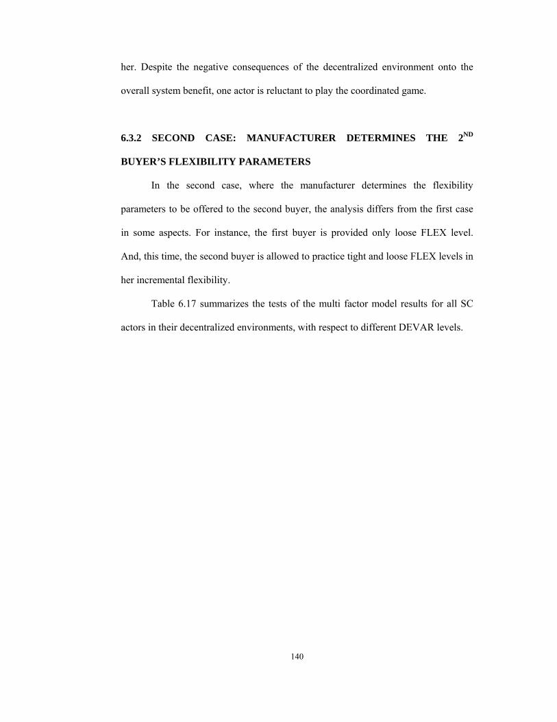
140

her. Despite the negative consequences of the decentralized environment onto the

overall system benefit, one actor is reluctant to play the coordinated game.

6.3.2 SECOND CASE: MANUFACTURER DETERMINES THE 2ND

BUYER’S FLEXIBILITY PARAMETERS

In the second case, where the manufacturer determines the flexibility

parameters to be offered to the second buyer, the analysis differs from the first case

in some aspects. For instance, the first buyer is provided only loose FLEX level.

And, this time, the second buyer is allowed to practice tight and loose FLEX levels in

her incremental flexibility.

Table 6.17 summarizes the tests of the multi factor model results for all SC

actors in their decentralized environments, with respect to different DEVAR levels.

141

Table 6.17 Cost Rankings and Comparison of Differences for SC Actors in the Decentralized Environment [Second Case]

Medium DEVAR High DEVAR DM

Cas

e

Envi

ronm

ent

SC A

ctor

FLEX(FB2,FM) COST (CB,CM) FLEX (FB2,FM) COST (CB,CM)

(H,*) (H,*)

(L,*) (L,*)

FIR

ST B

UY

ER

(T,*) (H,*) (T,*) (H,*)

(L,*) (L,*) (L,*) (L,*)

SEC

ON

D B

UY

ER

(T,T) (H,H) (T,T) (H,H)

(T,L) (L,H) (T,L) (L,H)

(L,T) (H,L) (L,T) (H,L)

(L,L) (L,L) (L,L) (L,L)

MA

NU

FAC

TUR

ER D

ETER

MIN

ES F

OR

2N

D B

UY

ER

DEC

ENTR

ALI

ZED

MA

NU

FAC

TUR

ER

* represents all different levels of the manufacturer

For the first buyer in her separate solution, there is no FLEX factor taken into

account, since she is provided only loose FLEX level. In high DEVAR, she is

indifferent in the COST levels, whereas in medium DEVAR, she has higher costs at

high levels of COST due to less uncertainty calling for the small differences in

quantities caused by the given loose FLEX level.

The second buyer has higher costs with respect to the first case, because this

time, the manufacturer determines the parameters, which are stated in Table E.1 in

Appendix E. She is provided tight and loose FLEX levels as presented in the

142

previous chapter. In medium DEVAR, she has less average costs at loose level of

FLEX. That is, her estimates fall within the bounds constructed by the flexibility

parameters, meaning that she gets the benefit of the flexibility option provided. She

is indifferent to both levels of COST at the two levels of DEVAR. According to the

Tukey’s test in the single factor model, in high DEVAR, the result indicates that she

is indifferent to all combinations of FLEX and COST levels. But, the results

according to the Duncan’s test in the single factor model and to both tests in the

multi factor model support the benefit gained due to the loose FLEX level by the

second buyer whatever the COST level is. All single factor model results in the

second case are presented in Appendix I.

Table 6.18 shows the different result of the Duncan’s test from Tukey’s test

for the manufacturer in the decentralized environment

Table 6.18 Different Results of Duncan’s Tests for the Manufacturer in the

Decentralized Environment

Medium DEVARD

M C

ase

Envi

ronm

ent

SC A

ctor

FLEX (FB2,FM)

(T,T)

(T,L)

(L,T)

(L,L)MA

NU

FAC

TUR

ER

DET

ERM

INES

FO

R 2

ND

BU

YER

CEN

TRA

LIZE

D

MA

NU

FAC

TUR

ER

The manufacturer in turn, has similar results as in the first case, where the

DM is the second buyer. Although he determines the flexibility parameters; in high

143

DEVAR, he doesn’t have differences in average costs as his incremental flexibility

parameters get looser. Since the parameters are determined to satisfy a total cost

limit, which is the optimal total cost of WCP obtained with the parameter decisions

neglected, the flexibility parameters are not sufficient to provide him with lower

average cost. However, in medium DEVAR, according to the results of Duncan’s

test applied in the multi factor model, which is presented in Table 6.18, the benefit

gained by the manufacturer due to the manufacturer’s loose FLEX is significant.

Similar to the first case results presented in Table 6.14, the high level of

COST absolutely results in high costs, at both DEVAR levels. Although the

inventory carrying and subcontracting costs gets high, the buyers do not change their

amounts of replenishments requested from the manufacturer, since they act all

independently from their own interests’ perspective.

In the integrated supply chain, the SC actors are concerned with all

combinations of the levels of FLEX and COST factors at a particular DEVAR level.

Although there is no loose or tight FLEX level distinction for the first buyer, in fact

the loose and tight FLEX levels of the second buyer and of the manufacturer affect

her.

The test results for SC actors in the centralized environment are presented in

Table 6.19.

144

Table 6.19 Cost Rankings and Comparison of Differences for SC Actors in the Centralized Environment [Second Case]

Medium DEVAR High DEVAR DM

Cas

e

Envi

ronm

ent

SC A

ctor

FLEX (FB2,FM) COST (CB,CM) FLEX (FB2,FM) COST (CB,CM) (T,T) (L,H) (L,T) (L,H)

(T,L) (H,H) (T,T) (H,H)

(L,L) (H,L) (T,L) (H,L)

(L,T) (L,L) (L,L) (L,L) FIR

ST B

UY

ER

(T,L) (L,H) (T,L) (L,H)

(T,T) (H,L) (T,T) (H,L)

(L,T) (H,H) (L,L) (L,L) (H,H)

(L,L) (L,L) (L,T) (L,L) SEC

ON

D B

UY

ER

(L,T) (H,H) (T,L) (H,H)

(L,L) (H,L) (L,T) (L,H)

(T,L) (L,H) (T,T) (H,L)

(T,T) (L,L) (L,L) (L,L)

MA

NU

FAC

TUR

ER D

ETER

MIN

ES F

OR

2N

D B

UY

ER

CEN

TRA

LIZE

D

MA

NU

FAC

TUR

ER

Unmatching results of Duncan’s test for the SC actors in the integrated supply

chain are presented in Table 6.20.

145

Table 6.20 Different Results of Duncan’s Tests for the SC Actors in the Centralized Environment [Second Case]

Medium DEVAR High DEVAR D

M C

ase

Envi

ronm

ent

SC A

ctor

FLEX (FB2,FM) COST (CB,CM) FLEX (FB2,FM) COST (CB,CM) (T,T) (L,H) (L,T) (L,H)

(T,L) (T,L) (H,H) (H,H) (T,T) (T,T) (H,H)

(L,L) (L,L) (H,L) (H,L) (T,L) (T,L) (H,L) (H,L)

(L,T) (L,L) (L,L) (L,L)FIR

ST B

UY

ER

(T,L)

(T,T) (T,T)

(L,L) (L,L)

(L,T) SEC

ON

D B

UY

ER

(H,H)

(L,H)

(H,L) (H,L)

(L,L)

MA

NU

FAC

TUR

ER D

ETER

MIN

ES F

OR

2N

D B

UY

ER

CEN

TRA

LIZE

D

MA

NU

FAC

TUR

ER

When the test results at both DEVAR levels are examined, it is observed that

the tight FLEX level of the manufacturer gives burden onto the first buyer. Also,

when this level is taken into account alone, it is seen that the loose FLEX level of the

second buyer also makes her cost higher. On the other hand, upon the loose FLEX

level of the manufacturer, the loose FLEX level of the second buyer grants benefit to

the first buyer since they are on the same side, i.e., they both request replenishment

from the manufacturer. Since the benefit arising from the loose FLEX level of the

146

manufacturer is directed to buyers in order to improve the systemwide performance,

when the second buyer is provided with loose FLEX level, the first buyer also gets

benefit from her loose FLEX level.

In high DEVAR, the first buyer has the highest average cost at the cost

combination (CB,CM)=(L,H) as in the first case. However, other (CB,CM)

combinations have unmatching outcomes in Tukey’s and Duncan’s tests. Tukey’s

test results in no different average costs for the cost combinations other than the

(CB,CM)=(L,H). Duncan’s test says that the low COST level of the manufacturer

yields significantly less average costs to the first buyer. In medium DEVAR, Tukey’s

test yields no difference for the average costs of the first buyer at all COST levels,

whereas Duncan’s test says the high COST level of the manufacturer results in

significantly higher cost for the first buyer than the low COST level of him. The

negative or positive effect of the manufacturer’s cost is all due to trying to direct his

cost burden onto the first buyer in order to make the system wide performance better.

However, the tests results are not decisive due to less number of samples. Thus,

lower error rate may be selected in determining the required sample size.

For the second buyer acting in integrated supply chain, the same results

gathered for the first buyer in the first case are obtained. The second buyer gets the

benefit as her flexibility parameters get looser while yielding better position not only

for her part but also in the overall system at both DEVAR levels. Also at either

DEVAR level, the (CB,CM)=(L,H) combination gives the highest average cost on the

second buyer as in the first buyer’s case. The reasoning behind this result is that in

order to reduce the subcontracting requirement due to the high subcontracting costs,

the buyers are forced to backorder some amount of their customer demand just to

147

improve the system wide performance. We also see that at high DEVAR level, the

second buyer wants the manufacturer be tight in his plans, while she maintains a

loose FLEX level. Since larger amount of the system wide cost is formed by the

manufacturer’s costs, she asks him to be tight and perform less subcontracting. In

medium DEVAR, she gets the most benefit when both parties have loose FLEX

levels due to less uncertainty, where the positive outcomes of flexibility usage can be

more easily captured.

The manufacturer, who plays his game with the buyers in the integrated

supply chain, is indifferent at all levels of FLEX at both DEVAR levels. Since he

determines the flexibility parameters with a limited total cost constraint, and since

the loose flexibility option is given to the first buyer at the beginning of the game,

being indifferent among FLEX levels is expected. Then, it can be concluded that the

system wide performance is based on the FLEX levels of the buyers, not of the

manufacturer. In high DEVAR, since there is no way to reduce the total system cost,

the highest average cost for the manufacturer occurs in the cost combination

(CB,CM)=(H,H), as expected. On the other hand, in the high DEVAR, Duncan’s test

indicates that the cost combinations, (L,H), (H,L) and (H,L), (L,L) are not

significantly different from each other, which means that his average cost can

decrease when there is some possibility for cost substitution among the buyers and

the manufacturer.

148

6.3.3 INDIVIDUAL versus INTEGRATED SUPPLY CHAIN

ENVIRONMENTS (Decentralized versus Centralized Environments)

Apart from the analysis of the factor levels on the attitudes of the SC actors,

and their underlying reasons in the individual and in the integrated supply chain

environments, the roles in playing the supply chain game separately or all together

are also investigated. In order to find out who wants to play on his own or who wants

to cooperate with the other parties, a single factor model where the factor

corresponds to being individual or being involved in the integrated supply chain is

constructed. For all SC actors, the single factor model is built for each combination

of FLEX and COST levels at a particular DEVAR level.

In the two cases, where the decision maker (DM) of the flexibility parameters

for the second buyer is alternated, combinations in which the first buyer favors

information asymmetry and in which she does not, are presented in Table 6.21 and

6.22. Favorable stands for support to be involved in the integrated supply chain,

unfavorable means the opposite, and no difference indicates the means of the

decentralized and centralized are not different.

149

Table 6.21 Decentralized versus Centralized Environments for the First Buyer in the First Case

2nd Buyer determines her flexibility parameters DEVAR: Medium/High ; FLEX: Tight/Loose ; COST: Low/High

FIRST BUYER FLEXIBILITY

TIGHTNESS (FB1,FM)COST

(CB,CM) Medium DEVAR High DEVAR

(L,L) - ο (L,H) - - (H,L) - ο

(T,T)

(H,H) - ο (L,L) - ο (L,H) - - (H,L) - ο

(T,L)

(H,H) - ο (L,L) - - (L,H) - - (H,L) - -

(L,T)

(H,H) - - (L,L) - - (L,H) - - (H,L) - -

(L,L)

(H,H) - - *: favorable -: unfavorable ο: no difference

As seen from the table, in the loose FLEX level, whether the first buyer has a

high or low COST level, she would never like to be involved in the integrated supply

chain at both DEVAR levels. Since risk increases at high DEVAR level, she tries to

carry more inventory for the future periods. Also, as the discrete possible demand

values are far apart from the forecast with this level of DEVAR, the chance of either

backordering or carrying large inventory increases. Thus, at high DEVAR level,

when she has tight FLEX level, she sometimes favors to be placed in the integrated

supply chain. On the other hand, in medium DEVAR, the case where she is provided

tight flexibility parameters, she has already got the advantage of flexibility options

due to less variation of her demand forecasts.

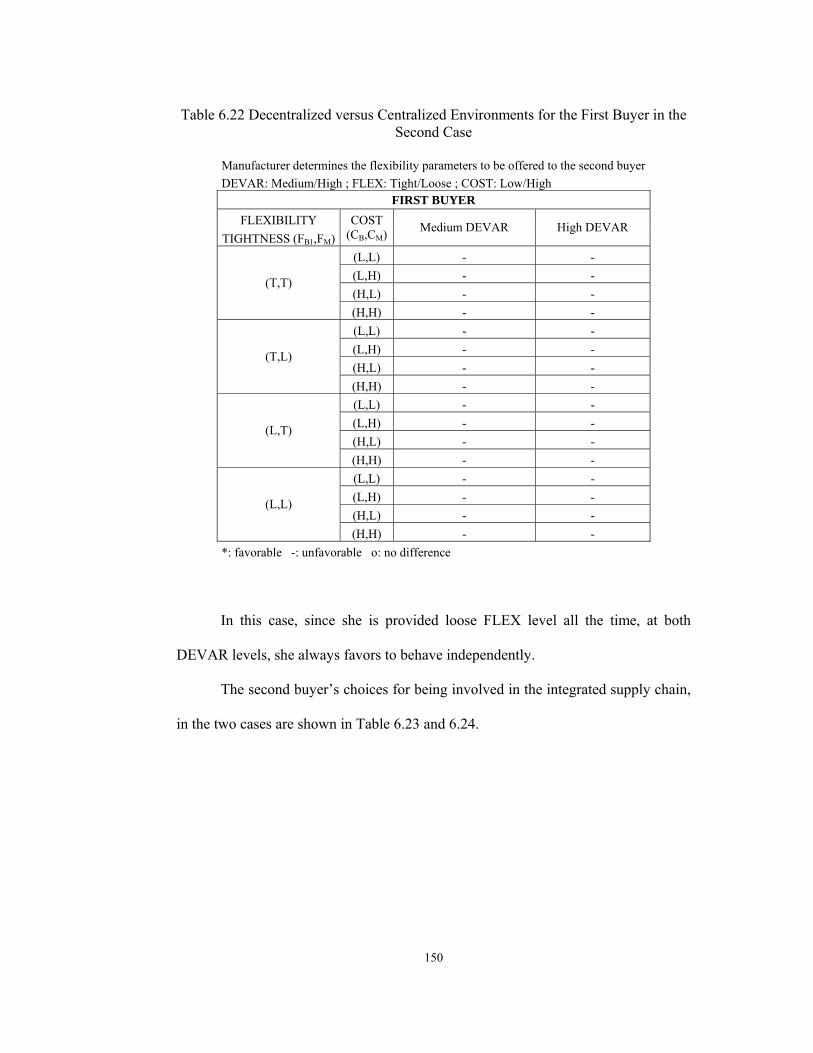
150

Table 6.22 Decentralized versus Centralized Environments for the First Buyer in the

Second Case

Manufacturer determines the flexibility parameters to be offered to the second buyer DEVAR: Medium/High ; FLEX: Tight/Loose ; COST: Low/High

FIRST BUYER FLEXIBILITY

TIGHTNESS (FB1,FM)COST

(CB,CM) Medium DEVAR High DEVAR

(L,L) - - (L,H) - - (H,L) - -

(T,T)

(H,H) - - (L,L) - - (L,H) - - (H,L) - -

(T,L)

(H,H) - - (L,L) - - (L,H) - - (H,L) - -

(L,T)

(H,H) - - (L,L) - - (L,H) - - (H,L) - -

(L,L)

(H,H) - - *: favorable -: unfavorable ο: no difference

In this case, since she is provided loose FLEX level all the time, at both

DEVAR levels, she always favors to behave independently.

The second buyer’s choices for being involved in the integrated supply chain,

in the two cases are shown in Table 6.23 and 6.24.

151

Table 6.23 Decentralized versus Centralized Environments for the Second Buyer in the First Case

2nd Buyer determines her flexibility parameters DEVAR: Medium/High ; FLEX: Tight/Loose ; COST: Low/High

SECOND BUYER FLEXIBILITY

TIGHTNESS (FB1,FM)COST

(CB,CM) Medium DEVAR High DEVAR

(L,L) ο ο (L,H) - - (H,L) ο ο

(T,T)

(H,H) ο ο (L,L) ο ο (L,H) - - (H,L) ο ο

(T,L)

(H,H) ο ο (L,L) ο ο (L,H) - - (H,L) ο -

(L,T)

(H,H) ο - (L,L) ο ο (L,H) - - (H,L) ο ο

(L,L)

(H,H) ο ο *: favorable -: unfavorable ο: no difference

Since the second buyer determines her flexibility parameters while

minimizing her inventory carrying and backordering costs; most of the time, she is

indifferent in behaving independently or not, at both DEVAR levels. She favors

being isolated at the cost combination (CB,CM) = (L,H). Because in the integrated

supply chain, the cost burden of the manufacturer is always directed to the buyers.

Apart from the particular cost combination, in high DEVAR, when she has loose

level of FLEX and the manufacturer has tight level of FLEX at (CB,CM)=(H,L) and

(H,H), she is again willing to behave independently, due to her high level of COST.

In her decentralized environment, she pays not too much for the high COST level,

152

although in the coordinated one, she pays more in order to make the overall system

benefit.

Table 6.24 Decentralized versus Centralized Environments for the Second Buyer in

the Second Case

Manufacturer determines the flexibility parameters to be offered to the second buyer DEVAR: Medium/High ; FLEX: Tight/Loose ; COST: Low/High

SECOND BUYER FLEXIBILITY

TIGHTNESS (FB1,FM)COST

(CB,CM) Medium DEVAR High DEVAR

(L,L) ο ο (L,H) - - (H,L) ο -

(T,T)

(H,H) ο ο (L,L) ο ο (L,H) - - (H,L) ο -

(T,L)

(H,H) ο ο (L,L) ο - (L,H) - - (H,L) ο -

(L,T)

(H,H) ο - (L,L) ο - (L,H) - - (H,L) ο -

(L,L)

(H,H) ο - *: favorable -: unfavorable ο: no difference

When she is offered the flexibility parameters determined by the

manufacturer, she is again indifferent to being involved in the integrated supply

chain or not, except in the cost combination of (CB,CM)=(L,H), with medium

DEVAR. This indicates that the manufacturer in fact offers sufficiently appealing

contract parameters. At high DEVAR level, she does not want to play all together,

because she is willing to use the advantage provided by the loose FLEX level, and

not to pay the cost burden of the manufacturer to put the system in a better position.

153

However, when she has tight FLEX, either with the cost burden given to both sides,

(H,H) or with low setting to all, (L,L); she is again indifferent at high DEVAR level.

This indicates that the COST level being different between the two sides does not

favor her to be involved in the centralized environment. That is, she gets the

advantage of her appealing contract parameters, when the costs are not different.

The manufacturer’s incentives related to behaving individually or not, in the

two different cases are similar to each other. Thus, the results are displayed together

in Table 6.25.

Table 6.25 Decentralized versus Centralized Environments for the Manufacturer in

the First and Second Cases

2nd Buyer determines her flexibility parameters Manufacturer determines the flexibility parameters to be offered to the second buyer DEVAR: Medium/High ; FLEX: Tight/Loose ; COST: Low/High

MANUFACTURER FLEXIBILITY

TIGHTNESS (FBb,FM)COST

(CB,CM) Medium DEVAR High DEVAR

(L,L) * * (L,H) * * (H,L) * *

(T,T)

(H,H) * * (L,L) * * (L,H) * * (H,L) * *

(T,L)

(H,H) * * (L,L) * * (L,H) * * (H,L) * *

(L,T)

(H,H) * * (L,L) * * (L,H) * * (H,L) * *

(L,L)

(H,H) * * *: favorable -: unfavorable ο: no difference For the first case, b=1 ; For the second case, b=2

154

As seen from the table, the manufacturer always wants to be involved in the

integrated supply chain. He would rather know every medium and short term

decisions of the buyers, and inform them what they request will cost to him directly,

i.e., subcontracting costs, to them and the overall system. Since he can know the

intended future replenishments, i.e., the internal self plans of the buyers; instead of

planning according to his own replenishment forecasts, management of his capacity

usage and subcontracting decisions according to the intended future replenishment

amounts will definitely favor him.

Different from the costs of the SC actors, the total system cost is also

statistically analyzed to examine whether to act in the decentralized or in the

centralized manner improves the overall system benefit. For the analysis, the models

are run based on each combination of the FLEX and COST levels at a particular

DEVAR level.

The tests results according to the two cases where the decision maker of the

flexibility parameters for the second buyer are different are presented in Table 6.26

and 6.27.

155

Table 6.26 Decentralized versus Centralized Environments for the Overall System in the First Case

2nd Buyer determines her flexibility parameters DEVAR: Medium/High ; FLEX: Tight/Loose ; COST: Low/High

OVERALL SYSTEM FLEXIBILITY

TIGHTNESS (FB1,FM)COST

(CB,CM) Medium DEVAR High DEVAR

(L,L) * * (L,H) * * (H,L) * *

(T,T)

(H,H) * * (L,L) * * (L,H) * * (H,L) * *

(T,L)

(H,H) * * (L,L) * * (L,H) * * (H,L) * *

(L,T)

(H,H) ο ο (L,L) * * (L,H) * * (H,L) * *

(L,L)

(H,H) ο ο *: favorable -: unfavorable ο: no difference

When the second buyer determines the flexibility parameters not considering

the others, it easily detected that, involving all SC actors into the supply chain game,

always favors the overall system benefit, except the cost combination (CB,CM)=(H,H)

upon the flexibility tightness combinations (FB,FM)=(L,T), (L,L). The reason for

the exception is that there is no way to reduce the overall cost, when the cost burden

is given to all the parties. The flexibility tightness exception stems from the fact that

the COST effect outweighs the FLEX effect. Although, the buyers get the benefit of

loose FLEX level, the manufacturer’s resulting cost offset their advantages. The

lesson from this is to enquire about the sources of costs to reap the benefits of

coordinated activity.

156

Table 6.27 Decentralized versus Centralized Environments for the Overall System in the Second Case

Manufacturer determines the flexibility parameters to be offered to the second buyer DEVAR: Medium/High ; FLEX: Tight/Loose ; COST: Low/High

OVERALL SYSTEM FLEXIBILITY

TIGHTNESS (FB2,FM)COST

(CB,CM) Medium DEVAR High DEVAR

(L,L) * * (L,H) * * (H,L) ο *

(T,T)

(H,H) ο * (L,L) * * (L,H) * * (H,L) ο ο

(T,L)

(H,H) ο * (L,L) ο * (L,H) * * (H,L) ο *

(L,T)

(H,H) ο * (L,L) ο * (L,H) * * (H,L) ο *

(L,L)

(H,H) ο * *: favorable -: unfavorable ο: no difference

When the manufacturer determines the flexibility parameters to be offered to

the second buyer, the overall system’s choice to involve all SC actors into the supply

chain game changes dramatically. Since the major part of the system cost is

comprised of the manufacturer’s inventory carrying and subcontracting cost, being

the DM makes the system behave like him, i.e., favoring integrated supply chain,

especially in high DEVAR. However, in medium DEVAR, at the cost combinations

(CB,CM)=(H,H), (H,L), the overall system is indifferent to the choice. Although the

buyers favor to be independent, i.e., in a decentralized manner; in medium DEVAR,

the high COST level of the manufacturer results in such a high cost that the overall

system cost gets high as in the integrated supply chain. Thus, due to less variation,

157

the system can not make itself better though information is fully shared. Moreover, at

the (H,L) combination, larger subcontracting amounts are realized due to high unit

cost of backordering in the centralized environment. In the decentralized

environment, though the high backordering cost doesn’t yield high costs for the

buyers, the subcontracting costs raised by the requested replenishment amounts cause

the overall system be indifferent in individual and integrated supply chain

environments. Whereas in high DEVAR, it can put itself in a better position by

involving all in a single game, since it has room to make possible adjustments in cost

substitution among SC actors such as using the flexibility options more efficiently.

That is, the higher the risk is, the more effectively the option is exploited.

158

CHAPTER VII

CONCLUSION

Demand forecast and volatility, inventory carrying, backordering, and

subcontracting costs, risk tolerance, capacity reservation, lead times are the drivers

that impact supply contracts

In this study, we aim to present a structure for the analysis of the incentives of

a buyer who is offered a Quantity Flexibility (QF) contract by a manufacturer having

a working QF contract with another buyer.

A QF contract is an arrangement that forces the parties plan more deliberately

to make the performance of not only theirs but also the overall system better. In this

particular type of contract, the buyer commits not to purchase less than a certain

percentage ω below her estimate and the manufacturer guarantees to release up to a

certain percentage α above her estimate. This feature of QF contract provides some

challenging effects such as less amount of inventory carried or demand backordered.

In this particular study, although the manufacturer has no relation with an

upstream supplier, he is treated as if he has a QF contract with himself. The aim is to

provide a QF environment to the manufacturer to manage his medium and short term

decisions with more control and deliberation.

The two buyers serve to their own markets and the manufacturer supplies the

same item to both buyers. All parties have their own forecast information with some

159

inaccuracy. Only the realized requirement for the current period and the

replenishment schedules for both buyers are informed to the manufacturer. The

manufacturer involved into the supply chain picture is given a limited capacity, but

also provided with two subcontracting options of different lead times.

The market demands and the actual replenishment amounts that the buyers

and the manufacturer face, are not deterministic. Hence, the models constructed for

all parties with the objective of cost minimization turns out to be stochastic models.

In the formulation of these stochastic models, a scenario based approach is utilized.

In these models, some decision variables are independent and some are dependent on

the realizations of the random variables. The former ones are called “here and now”

decisions, and the latter ones are called “wait and see” decisions. The model is

divided into two stages, where the independent and the dependent decision variables

are in the first and second stages, respectively. The two-stage stochastic models of all

parties are solved using Benders Decomposition algorithm.

We analyze the attitudes of the SC actors in both the individual and the

integrated supply chain environments, where there is no information asymmetry in

the latter. For the analysis, three factors are decided to apply, which are demand

variation, DEVAR, flexibility tightness, FLEX, and cost, COST. The values of these

particular factor levels are determined with the approach of being at the reasonable

minimum and maximum extremes.

Moreover, two main cases related to the second buyer are generated. In the

first case, the decision maker (DM) of the flexibility parameters to be used by the

second buyer is herself, whereas in the second case the DM is the manufacturer.

According to these two cases, at different factor levels, the incentives of all SC actors

160

in their individual, i.e., decentralized and in the integrated supply chain, i.e.,

centralized environments are questioned.

For the analysis some samples are taken from the possible scenarios

generated which are not identical for the buyers and the manufacturer. According to

the results of these samples, multiple comparisons are carried out by utilizing the

statistical software, SAS, with the multiple test options it provides. The Tukey’s and

Duncan’s tests are applied for the comparisons, where the former evaluates the Type

I experiment wise error rate, and the latter, comparison wise error rate.

In accordance with the multiple test results, it can be concluded that in the

first case, the second buyer is indifferent to behave independently or be involved in

the integrated supply chain due to being the DM of her flexibility parameters. That

is, she gets the advantage of the flexibility option provided by the QF contract. In the

second case, she is mostly indifferent in medium DEVAR, indicating that the

flexibility parameters offered to her are sufficiently appealing. However, in high

DEVAR, she favors begin independent due to increasing uncertainty.

In both cases, the first buyer often favors being alone in the QF environment.

Since she is given the flexibility parameters beforehand, she always exploits the

flexibility option provided when she is on her own. However, when she is involved

into the integrated supply chain, she is always given the cost burden of the

manufacturer and sometimes of the second buyer, too.

Moreover, at either DEVAR levels, the cost combination (CB,CM)=(L,H)

gives the highest cost for the two buyers in the centralized environment. This is due

to the high cost of subcontracting. Since the aim is to improve the systemwide

performance, in order not to give larger orders to the subcontractor, the buyers are

161

forced to backorder some amount of their customer demand. Since the high COST of

the manufacturer results in high average costs for him and the integrated SC, when a

cost reduction program is activated, it should start at the manufacturer.

However, the manufacturer is willing to be involved in the integrated supply

chain all the time and in all different environmental factors. This typical behavior is

due to the limited capacity, and the expensive subcontracting option. Especially, as

the demand variation increases, i.e., uncertainty increases, the willingness to have the

information of the others’ decisions and to inform others of his, increases.

Less variation in the replenishment forecasts, i.e., medium DEVAR yields in

less subcontracting, less inventory carried for the future periods, and high capacity

utilization. This is also achieved by the loose FLEX of the buyers resulting less

replenishment amounts requested from him. Thus, the manufacturer gets into a better

position in his individual environment, when the buyers also get the benefit of loose

FLEX and low COST, and then request less. However, the marginal improvement is

not as big as the one in the integrated supply chain. Since the manufacturer has a

limited capacity, i.e., he has a restricted environment, he has to do subcontracting.

Some part of the cost of this compulsion can be directed to others in the integrated

supply chain environment which results in less cost than in his individual

environment.

It is also observed that in some cases, the limited capacity of the manufacturer

is not utilized in full. Due to the intention to cover all forecasted replenishments,

larger amounts are ordered to the subcontractor. When a relatively less replenishment

amount is realized, the excess subcontracting amount arrives regardless of the actual

need which reduces the capacity utilization.

162

Another characteristic result is that as the demand variation increases, the

values of the flexibility parameters of the second buyer increase in both cases. This

indicates that as uncertainty increases, the willingness to have more flexibility option

and worth of flexibility increase in order to offset the variation effect by the

opportunities provided.

Moreover, when the DM is the manufacturer, the system model often

suggests similar decisions as to being independent or not, as the manufacturer. Due

to being the creator of the environment characteristics, the system behaves like him.

Furthermore, in medium DEVAR, the positive outcomes of the flexibility

usage can be more easily captured due to lower uncertainty, i.e., less possibility for

the realizations of large and small demands or replenishments. It can also be

concluded that the system wide performance is mostly based on the FLEX levels of

the buyers, not of the manufacturer in both cases.

Additionally, although the buyers favor to be independent, i.e., in a

decentralized manner; in medium DEVAR; the high COST level of the manufacturer

results in such a high cost that the overall system cost gets high as in the integrated

supply chain. Thus, due to less variation, the system can not make itself better though

information is fully shared. Whereas in high DEVAR, it can put itself in a better

position in the centralized environment due to information sharing and control. That

is, the higher the risk is, the more effectively the option is exploited for the overall

system.

It is also observed that information sharing gives benefit to the overall system

most of the time. This also indicates that apart from the involvers of the QF contract

who are the buyers and the manufacturer, also the customers can take a part in the

163

contracts, so that more accurate information will be gathered, which will definitely

improve the system.

In this study, the stochastic random variables are assumed to have discrete

distributions to avoid nonlinearities. As a future research, they can be assumed to

have continuous distributions, and instead of struggling with the nonlinearities, some

heuristic approaches can be generated.

Another future research direction can be the analysis of the limited capacity

amount and trying to figure out at which level, the manufacturer can exploit the

flexibility option while taking the buyers’ choices into account. Also, the tradeoff

between having a limited capacity and investing for the expansion of the restricted

capacity can be investigated.

Moreover, what rations the limited capacity of the manufacturer, the effect of

the flexibility given for each buyer on the capacity allocation, and ways to coordinate

for the limited capacity can be the possible future research questions.

Game theoretic approaches may be applied between the two buyers and

between one buyer and the manufacturer to analyze the attitudes and the possible

negotiations opportunities. Also the buyers can incorporate within each other by

informing some part of their decisions to the other one to utilize the limited capacity,

and hence improve the performance of both.

Finally, for continuous probability distributions, Monte Carlo sampling and

Gaussian quadrature, which are the two most commonly used discreatization

stragtegies can be applied for the probability space for approximating the

multivariate probability integrals.

164

Moreover, some comparison test results do not agree, i.e., are inconclusive to

decide which factor affects the others or the reasoning underlying the consequences.

To overcome the indecisiveness of the test results, sample size can be increased for

the analysis. That is, the error rate in selecting the required sample size may be

decreased as a future research.

165

REFERENCES

[1] Anupindi, R., and Bassok, Y. (1998b), “Supply Contracts with Quantity Commitments and Stochastic Demand”. In S. Tayur, M. Magazine, and R. Ganeshan, Quantitative Models for Supply Chain Management, Kluwer Academic Publishers.

[2] Barnes-Schuster, D., Bassok, Y., and Anupindi, R. (2000), “Coordination and Flexibility in Supply Contracts with Options”. Working Paper, University of Chicago, under review for Journal of MSOM.

[3] Bassok, Y., and Anupindi, R. (1997), “Analysis of Supply Contracts with Total Minimum Commitment”. IIE Transactions, Vol. 28, 373-381.

[4] Bassok, Y., and Anupindi, R. (1998), “Analysis of Supply Contracts with Commitments and Flexibility”. Working Paper, Northwestern University.

[5] Bassok, Y., Bixby, A., Srinivasan, R., and Wiesel, H.Z. (1998), “Design of Component-Supply Contract with Commitment-Revision Flexibility”. Journal of Research and Development, Vol. 41, No. 6, 693-705.

[6] Birge, J. R. (1997), “Stochastic Programming Computation and applications”. INFORMS Journal of Computing, Vol. 9, No. 9, 111-133.

[7] Brown, A. O., and Lee, H. L. (2000), “The Impact of Demand Signal Quality on Optimal Decisions in Supply Contracts”. Working Paper, Vanderbilt University, Nashville, TN.

[8] Chen, F. Y., and Krass, D. (2001), “Analysis of Supply Contracts with Minimum Total Order Quantity Commitments and Non-Stationary Demands”. European Journal of Operational Research, Vol. 131, 309-323.

166

[9] Chen, Z., Li, S., and Tirupati, D. (2002), “A Scenario-based Stochastic Programming Approach for Technology and Capacity Planning”. Computers and Operations Research, Vol. 29, 781-806. [10] Delft, Ch. Van., and Vial, J.-Ph. (2001), “Quantitative Analysis of Multi-Periodic Supply Chain Contracts with Options via Stochastic Programming”. Working Paper, Department of Management Studies, University of Geneva.

[11] Eppen, G. D., and Iyer, A. V. (1997), “Backup Agreements in Fashion Buying-The Value of Upstream Flexibility”. Management Science, Vol. 43, No. 11, 1469-1484.

[12] Erkoc, M., and Wu, S. D. (2002), “Managing High-Tech Capacity Expansion via Reservation Contracts”. Working Paper, P. C. Rossin College of Engineering, Lehigh University, Bethlehem, PA.

[13] Gupta, A., and Maranas, C. D. (2000), “A Two-Stage Modeling and Solution Framework for Multisite Midterm Planning under Demand Uncertainty”. Industrial and Engineering Chemistry Research, Vol. 39, 3799-3813.

[14] Gupta, A., Maranas, C. D., and McDonald, C. M. (2000), “Mid-term Supply Chain Planning under Demand Uncertainty: Customer Demand Satisfaction and Inventory Management”. Computers and Chemical Engineering, Vol. 24, 2613-2621.

[15] Huang, H., Sethi, S. P., and Yan, H. (2002), “Purchase Contract Management with Demand Forecast Updates”. IIE Transaction: Scheduling and Logistics, under review.

[16] Li, C., and Kouvelis, P. (1999), “Flexible and Risk-Sharing Supply Contracts under Price Uncertainty”. Management Science, Vol. 45, No. 10, 1378-1398.

[17] Liu, M. L., and Sahinidis, N. V. (1996), “Optimization in Process Planning under Uncertainty”. Ind. Eng. Chem. Res., Vol. 35, 4154-4165.

[18] Milner, J. M., and Rosenblatt, M. J. (1997), “Two Period Supply Contracts: Order Adjustments and Penalties”. Working Paper, Olin School of Business, University of Washington.

167

[19] Plambeck, E. L., and Taylor, T. A. (2002), “Renegotiation of Supply Contracts”. Stanford Graduate School of Business Research Paper Series, Research Paper No.1764, submitted to Management Science.

[20] Schweitzer, E. (1994), “Multi-stage Mathematical Modeling under Uncertainty”. Research Thesis, Israel Institute of Technology.

[21] Spinler, S., Huchzermeir, A., and Kleindorfer, P. R. (2002), “The Valuation of Options on Capacity”. Working Paper, submitted to Management Science.

[22] Tsay, A. A., and Lovejoy, W. S. (1999), “Quantity Flexibility Contracts and Supply Chain Performance”. Manufacturing and Service Operations Management, Vol. 1, No. 2, 89-111.

[23] Tsay, A. A. (1999), “The Quantity Flexibility Contract and Supplier-Customer Incentives”. Management Science, Vol. 45, No. 10, 1339-1358.

168

APPENDIX A

DEMAND DATA GENERATED FOR THE FIRST AND SECOND

BUYERS IN MEDIUM ANG HIGH DEVAR

Table A.1 Demand Data Generated for the First Buyer in Medium DEVAR

1ST BUYER MEDIUM DEVAR Discrete Values Probabilities 1ST PERIOD 500 2ND PERIOD 605 0.3 495 0.1 575 0.2 510 0.4 MEAN 550 3RD PERIOD 660 0.2 540 0.3 520 0.1 635 0.4 MEAN 600 4TH PERIOD 615 0.3 485 0.1 585 0.2 500 0.4 MEAN 550 2ND PERIOD 3RD PERIOD 660 0.2 540 0.3 560 0.1 625 0.4 MEAN 600 4TH PERIOD 605 0.3 495 0.1 595 0.2 500 0.4 MEAN 550 5TH PERIOD 660 0.2 600 540 0.3 500 0.1 640 0.4 MEAN 600

169

1ST BUYER Discrete Values Probabilities 3RD PERIOD 4TH PERIOD 605 0.3 495 0.1 575 0.2 510 0.4 MEAN 550 5TH PERIOD 660 0.2 540 0.3 520 0.1 635 0.4 MEAN 600 6TH PERIOD 615 0.3 550 485 0.1 585 0.2 500 0.4 MEAN 550 4TH PERIOD 5TH PERIOD 660 0.2 540 0.3 560 0.1 625 0.4 MEAN 600 6TH PERIOD 605 0.3 495 0.1 595 0.2 500 0.4 MEAN 550 7TH PERIOD 555 0.1 500 445 0.3 455 0.2 550 0.4 MEAN 500

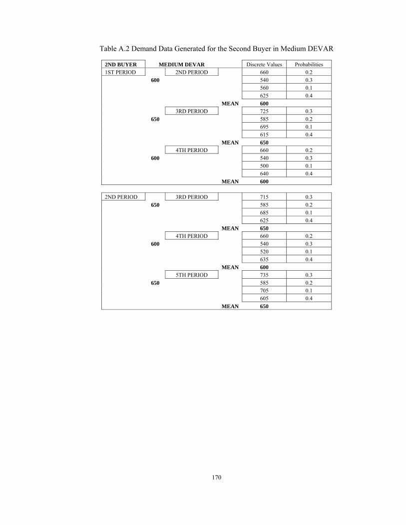
170

Table A.2 Demand Data Generated for the Second Buyer in Medium DEVAR

2ND BUYER MEDIUM DEVAR Discrete Values Probabilities 1ST PERIOD 2ND PERIOD 660 0.2 600 540 0.3 560 0.1 625 0.4 MEAN 600 3RD PERIOD 725 0.3 650 585 0.2 695 0.1 615 0.4 MEAN 650 4TH PERIOD 660 0.2 600 540 0.3 500 0.1 640 0.4 MEAN 600 2ND PERIOD 3RD PERIOD 715 0.3 650 585 0.2 685 0.1 625 0.4 MEAN 650 4TH PERIOD 660 0.2 600 540 0.3 520 0.1 635 0.4 MEAN 600 5TH PERIOD 735 0.3 650 585 0.2 705 0.1 605 0.4 MEAN 650

171

2ND BUYER Discrete Values Probabilities 3RD PERIOD 4TH PERIOD 660 0.2 600 540 0.3 560 0.1 625 0.4 MEAN 600 5TH PERIOD 725 0.3 650 585 0.2 695 0.1 615 0.4 MEAN 650 6TH PERIOD 660 0.2 600 540 0.3 500 0.1 640 0.4 MEAN 600 4TH PERIOD 5TH PERIOD 715 0.3 650 585 0.2 685 0.1 625 0.4 MEAN 650 6TH PERIOD 660 0.2 600 540 0.3 520 0.1 635 0.4 MEAN 600 7TH PERIOD 615 0.3 550 485 0.1 585 0.2 500 0.4 MEAN 550

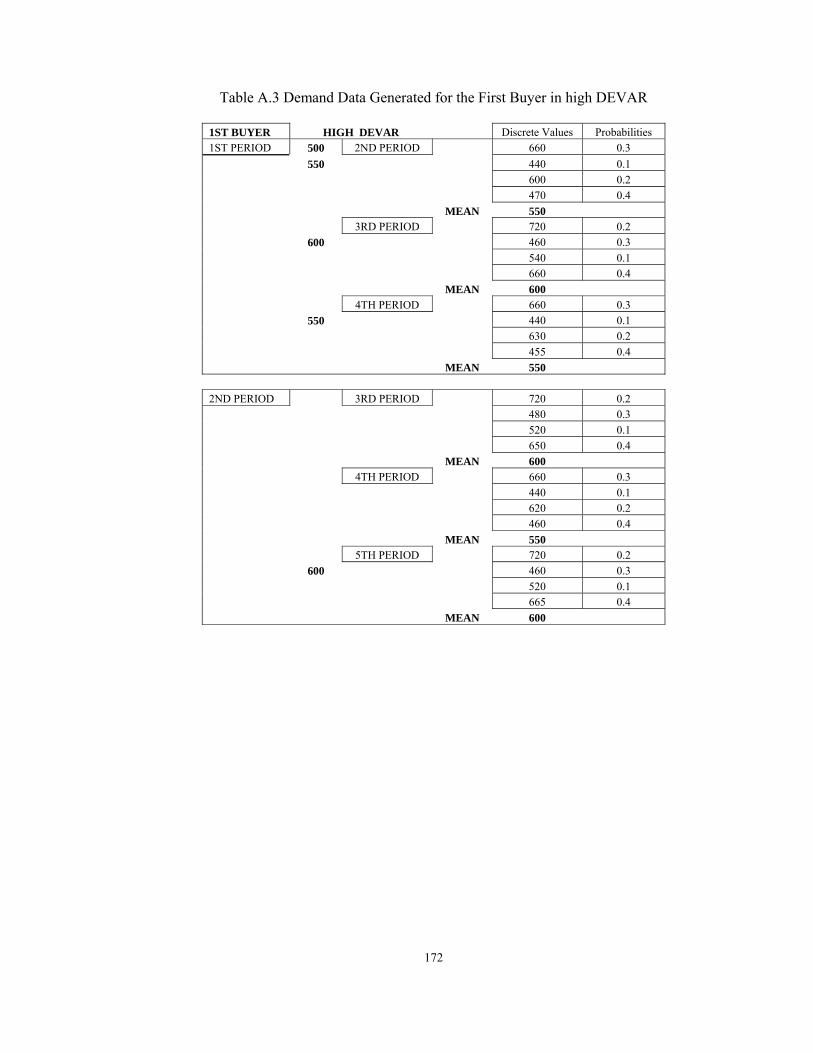
172

Table A.3 Demand Data Generated for the First Buyer in high DEVAR

1ST BUYER HIGH DEVAR Discrete Values Probabilities 1ST PERIOD 500 2ND PERIOD 660 0.3 550 440 0.1 600 0.2 470 0.4 MEAN 550 3RD PERIOD 720 0.2 600 460 0.3 540 0.1 660 0.4 MEAN 600 4TH PERIOD 660 0.3 550 440 0.1 630 0.2 455 0.4 MEAN 550 2ND PERIOD 3RD PERIOD 720 0.2 480 0.3 520 0.1 650 0.4 MEAN 600 4TH PERIOD 660 0.3 440 0.1 620 0.2 460 0.4 MEAN 550 5TH PERIOD 720 0.2 600 460 0.3 520 0.1 665 0.4 MEAN 600

173

1ST BUYER Discrete Values Probabilities 3RD PERIOD 4TH PERIOD 660 0.3 440 0.1 600 0.2 470 0.4 MEAN 550 5TH PERIOD 720 0.2 460 0.3 540 0.1 660 0.4 MEAN 600 6TH PERIOD 660 0.3 550 440 0.1 630 0.2 455 0.4 MEAN 550 4TH PERIOD 5TH PERIOD 720 0.2 480 0.3 520 0.1 650 0.4 MEAN 600 6TH PERIOD 660 0.3 440 0.1 620 0.2 460 0.4 MEAN 550 7TH PERIOD 600 0.1 500 400 0.3 420 0.2 590 0.4 MEAN 500

174

Table A.4 Demand Data Generated for the Second Buyer in High DEVAR

2ND BUYER HIGH DEVAR Discrete Values Probabilities 1ST PERIOD 2ND PERIOD 720 0.2 600 480 0.3 520 0.1 650 0.4 MEAN 600 3RD PERIOD 800 0.3 650 520 0.2 700 0.1 590 0.4 MEAN 650 4TH PERIOD 720 0.2 600 460 0.3 520 0.1 665 0.4 MEAN 600 2ND PERIOD 3RD PERIOD 780 0.3 650 520 0.2 740 0.1 595 0.4 MEAN 650 4TH PERIOD 720 0.2 600 460 0.3 540 0.1 660 0.4 MEAN 600 5TH PERIOD 800 0.3 650 520 0.2 760 0.1 575 0.4 MEAN 650

175

2ND BUYER Discrete Values Probabilities 3RD PERIOD 4TH PERIOD 720 0.2 480 0.3 520 0.1 650 0.4 MEAN 600 5TH PERIOD 800 0.3 520 0.2 700 0.1 590 0.4 MEAN 650 6TH PERIOD 720 0.2 600 460 0.3 520 0.1 665 0.4 MEAN 600 4TH PERIOD 5TH PERIOD 780 0.3 650 520 0.2 740 0.1 595 0.4 MEAN 650 6TH PERIOD 720 0.2 600 460 0.3 540 0.1 660 0.4 MEAN 600 7TH PERIOD 660 0.3 550 440 0.1 630 0.2 455 0.4 MEAN 550

176

APPENDIX B

DEMAND DATA GENERATED FOR THE MANUFACTURER IN

MEDIUM AND HIGH DEVAR

Table B.1 Demand Data Generated for the Manufacturer in Medium DEVAR

MANUFACTURER FOR 1ST BUYER MEDIUM DEVAR Discrete Values Probabilities 1ST PERIOD 2ND PERIOD 605 0.2 550 495 0.3 525 0.1 570 0.4 MEAN 550 3RD PERIOD 660 0.3 600 540 0.1 550 0.4 640 0.2 MEAN 600 4TH PERIOD 605 0.2 550 475 0.3 505 0.1 590 0.4 MEAN 550 MANUFACTURER FOR 2ND BUYER Discrete Values Probabilities 1ST PERIOD 2ND PERIOD 660 0.3 600 540 0.1 560 0.4 620 0.2 MEAN 600 3RD PERIOD 715 0.1 650 585 0.3 595 0.2 710 0.4 MEAN 650 4TH PERIOD 660 0.3 600 530 0.1 545 0.4 655 0.2 MEAN 600

177

MANUFACTURER FOR 1ST BUYER Discrete Values Probabilities 2ND PERIOD 3RD PERIOD 660 0.3 540 0.1 560 0.4 620 0.2 MEAN 600 4TH PERIOD 605 0.2 485 0.3 495 0.1 585 0.4 MEAN 550 5TH PERIOD 660 0.3 600 530 0.1 545 0.4 655 0.2 MEAN 600 MANUFACTURER FOR 2ND BUYER Discrete Values Probabilities 2ND PERIOD 3RD PERIOD 715 0.1 585 0.3 615 0.2 700 0.4 MEAN 650 4TH PERIOD 660 0.3 540 0.1 550 0.4 640 0.2 MEAN 600 5TH PERIOD 725 0.1 650 565 0.3 630 0.2 705 0.4 MEAN 650

178

MANUFACTURER FOR 1ST BUYER Discrete Values Probabilities 3RD PERIOD 4TH PERIOD 605 0.2 495 0.3 525 0.1 570 0.4 MEAN 550 5TH PERIOD 660 0.3 540 0.1 550 0.4 640 0.2 MEAN 600 6TH PERIOD 605 0.2 550 475 0.3 505 0.1 590 0.4 MEAN 550 MANUFACTURER FOR 2ND BUYER Discrete Values Probabilities 3RD PERIOD 4TH PERIOD 660 0.3 540 0.1 560 0.4 620 0.2 MEAN 600 5TH PERIOD 715 0.1 585 0.3 595 0.2 710 0.4 MEAN 650 6TH PERIOD 660 0.3 600 530 0.1 545 0.4 655 0.2 MEAN 600

179

MANUFACTURER FOR 1ST BUYER Discrete Values Probabilities 4TH PERIOD 5TH PERIOD 660 0.3 540 0.1 560 0.4 620 0.2 MEAN 600 6TH PERIOD 605 0.2 485 0.3 495 0.1 585 0.4 MEAN 550 7TH PERIOD 565 0.3 500 420 0.2 485 0.1 495 0.4 MEAN 500 MANUFACTURER FOR 2ND BUYER Discrete Values Probabilities 4TH PERIOD 5TH PERIOD 715 0.1 585 0.3 615 0.2 700 0.4 MEAN 650 6TH PERIOD 660 0.3 540 0.1 550 0.4 640 0.2 MEAN 600 7TH PERIOD 605 0.2 550 475 0.3 505 0.1 590 0.4 MEAN 550

180

Table B.2 Demand Data Generated for the Manufacturer in High DEVAR

MANUFACTURER FOR 1ST BUYER HIGH

DEVAR Discrete Values Probabilities 1ST PERIOD 2ND PERIOD 660 0.2 550 440 0.3 480 0.1 595 0.4 MEAN 550 3RD PERIOD 720 0.3 600 480 0.1 505 0.4 670 0.2 MEAN 600 4TH PERIOD 660 0.2 550 420 0.3 460 0.1 615 0.4 MEAN 550 MANUFACTURER FOR 2ND BUYER Discrete Values Probabilities 1ST PERIOD 2ND PERIOD 720 0.3 600 480 0.1 515 0.4 650 0.2 MEAN 600 3RD PERIOD 780 0.1 650 520 0.3 580 0.2 750 0.4 MEAN 650 4TH PERIOD 720 0.3 600 480 0.1 500 0.4 680 0.2 MEAN 600

181

MANUFACTURER FOR 1ST BUYER Discrete Values Probabilities 2ND PERIOD 3RD PERIOD 720 0.3 600 480 0.1 515 0.4 650 0.2 MEAN 600 4TH PERIOD 660 0.2 550 420 0.3 500 0.1 605 0.4 MEAN 550 5TH PERIOD 720 0.3 600 480 0.1 500 0.4 680 0.2 MEAN 600 MANUFACTURER FOR 2ND BUYER Discrete Values Probabilities 2ND PERIOD 3RD PERIOD 780 0.1 650 520 0.3 600 0.2 740 0.4 MEAN 650 4TH PERIOD 720 0.3 600 480 0.1 505 0.4 670 0.2 MEAN 600 5TH PERIOD 780 0.1 650 520 0.3 560 0.2 760 0.4 MEAN 650

182

MANUFACTURER FOR 1ST BUYER Discrete Values Probabilities 3RD PERIOD 4TH PERIOD 660 0.2 550 440 0.3 480 0.1 595 0.4 MEAN 550 5TH PERIOD 720 0.3 600 480 0.1 505 0.4 670 0.2 MEAN 600 6TH PERIOD 660 0.2 550 420 0.3 460 0.1 615 0.4 MEAN 550 MANUFACTURER FOR 2ND BUYER Discrete Values Probabilities 3RD PERIOD 4TH PERIOD 720 0.3 600 480 0.1 515 0.4 650 0.2 MEAN 600 5TH PERIOD 780 0.1 650 520 0.3 580 0.2 750 0.4 MEAN 650 6TH PERIOD 720 0.3 600 480 0.1 500 0.4 680 0.2 MEAN 600

183

MANUFACTURER FOR 1ST BUYER Discrete Values Probabilities 4TH PERIOD 5TH PERIOD 720 0.3 600 480 0.1 515 0.4 650 0.2 MEAN 600 6TH PERIOD 660 0.2 550 420 0.3 500 0.1 605 0.4 MEAN 550 7TH PERIOD 620 0.3 500 400 0.2 580 0.1 440 0.4 MEAN 500 MANUFACTURER FOR 2ND BUYER Discrete Values Probabilities 4TH PERIOD 5TH PERIOD 780 0.1 650 520 0.3 600 0.2 740 0.4 MEAN 650 6TH PERIOD 720 0.3 600 480 0.1 505 0.4 670 0.2 MEAN 600 7TH PERIOD 660 0.2 550 420 0.3 460 0.1 615 0.4 MEAN 550

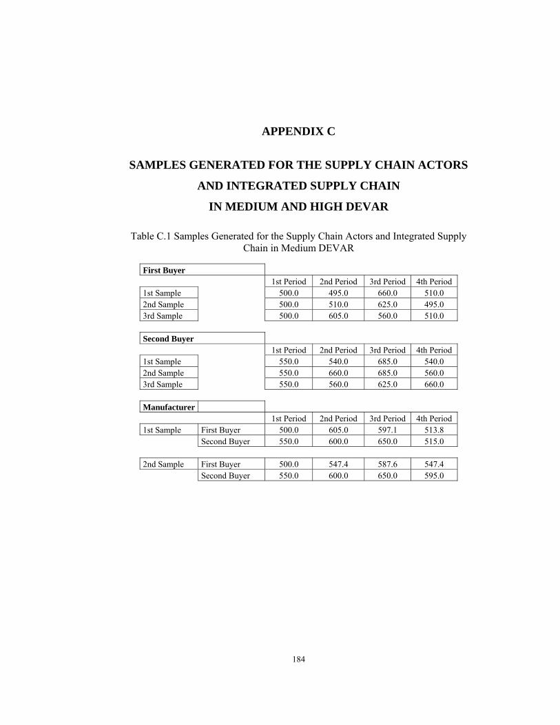
184

APPENDIX C

SAMPLES GENERATED FOR THE SUPPLY CHAIN ACTORS

AND INTEGRATED SUPPLY CHAIN

IN MEDIUM AND HIGH DEVAR

Table C.1 Samples Generated for the Supply Chain Actors and Integrated Supply

Chain in Medium DEVAR

First Buyer 1st Period 2nd Period 3rd Period 4th Period 1st Sample 500.0 495.0 660.0 510.0 2nd Sample 500.0 510.0 625.0 495.0 3rd Sample 500.0 605.0 560.0 510.0 Second Buyer 1st Period 2nd Period 3rd Period 4th Period 1st Sample 550.0 540.0 685.0 540.0 2nd Sample 550.0 660.0 685.0 560.0 3rd Sample 550.0 560.0 625.0 660.0 Manufacturer 1st Period 2nd Period 3rd Period 4th Period 1st Sample First Buyer 500.0 605.0 597.1 513.8 Second Buyer 550.0 600.0 650.0 515.0 2nd Sample First Buyer 500.0 547.4 587.6 547.4 Second Buyer 550.0 600.0 650.0 595.0

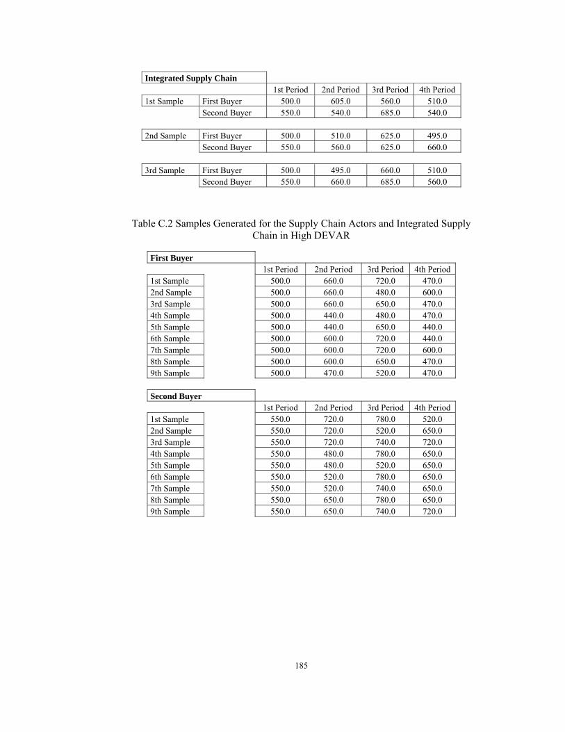
185

Integrated Supply Chain 1st Period 2nd Period 3rd Period 4th Period 1st Sample First Buyer 500.0 605.0 560.0 510.0 Second Buyer 550.0 540.0 685.0 540.0 2nd Sample First Buyer 500.0 510.0 625.0 495.0 Second Buyer 550.0 560.0 625.0 660.0 3rd Sample First Buyer 500.0 495.0 660.0 510.0 Second Buyer 550.0 660.0 685.0 560.0

Table C.2 Samples Generated for the Supply Chain Actors and Integrated Supply Chain in High DEVAR

First Buyer 1st Period 2nd Period 3rd Period 4th Period 1st Sample 500.0 660.0 720.0 470.0 2nd Sample 500.0 660.0 480.0 600.0 3rd Sample 500.0 660.0 650.0 470.0 4th Sample 500.0 440.0 480.0 470.0 5th Sample 500.0 440.0 650.0 440.0 6th Sample 500.0 600.0 720.0 440.0 7th Sample 500.0 600.0 720.0 600.0 8th Sample 500.0 600.0 650.0 470.0 9th Sample 500.0 470.0 520.0 470.0 Second Buyer 1st Period 2nd Period 3rd Period 4th Period 1st Sample 550.0 720.0 780.0 520.0 2nd Sample 550.0 720.0 520.0 650.0 3rd Sample 550.0 720.0 740.0 720.0 4th Sample 550.0 480.0 780.0 650.0 5th Sample 550.0 480.0 520.0 650.0 6th Sample 550.0 520.0 780.0 650.0 7th Sample 550.0 520.0 740.0 650.0 8th Sample 550.0 650.0 780.0 650.0 9th Sample 550.0 650.0 740.0 720.0

186

Manufacturer 1st Period 2nd Period 3rd Period 4th Period 1st Sample First Buyer 500.0 612.5 714.5 622.7 Second Buyer 550.0 720.0 650.0 520.0 2nd Sample First Buyer 500.0 612.5 646.5 552.2 Second Buyer 550.0 720.0 740.0 719.9 3rd Sample First Buyer 500.0 612.5 697.9 597.1 Second Buyer 550.0 600.0 660.0 650.0 4th Sample First Buyer 500.0 553.9 573.3 529.5 Second Buyer 550.0 600.0 700.0 650.0 5th Sample First Buyer 500.0 553.9 573.3 541.0 Second Buyer 550.0 600.0 650.0 400.0 6th Sample First Buyer 500.0 600.0 714.5 597.1 Second Buyer 550.0 650.0 740.0 719.9 7th Sample First Buyer 500.0 600.0 714.5 605.5 Second Buyer 550.0 650.0 780.0 650.0 8th Sample First Buyer 500.0 600.0 650.0 595.4 Second Buyer 550.0 720.0 780.0 520.0 9th Sample First Buyer 500.0 553.9 573.3 529.5 Second Buyer 550.0 600.0 660.0 650.0

187

Integrated Supply Chain 1st Period 2nd Period 3rd Period 4th Period 1st Sample First Buyer 500.0 660.0 720.0 470.0 Second Buyer 550.0 720.0 520.0 650.0 2nd Sample First Buyer 500.0 660.0 480.0 600.0 Second Buyer 550.0 720.0 740.0 720.0 3rd Sample First Buyer 500.0 660.0 650.0 470.0 Second Buyer 550.0 480.0 780.0 650.0 4th Sample First Buyer 500.0 440.0 480.0 470.0 Second Buyer 550.0 520.0 780.0 650.0 5th Sample First Buyer 500.0 440.0 650.0 440.0 Second Buyer 550.0 480.0 520.0 650.0 6th Sample First Buyer 500.0 600.0 720.0 440.0 Second Buyer 550.0 650.0 740.0 720.0 7th Sample First Buyer 500.0 600.0 720.0 600.0 Second Buyer 550.0 650.0 780.0 650.0 8th Sample First Buyer 500.0 600.0 650.0 470.0 Second Buyer 550.0 720.0 780.0 520.0 9th Sample First Buyer 500.0 470.0 520.0 470.0 Second Buyer 550.0 520.0 740.0 650.0

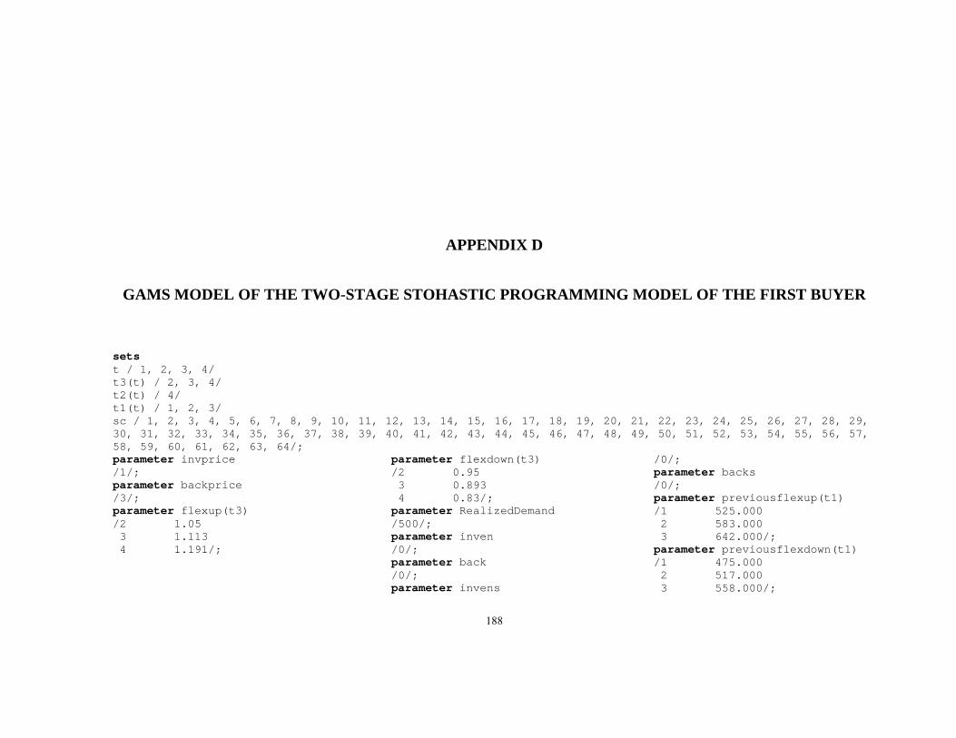
188

APPENDIX D

GAMS MODEL OF THE TWO-STAGE STOHASTIC PROGRAMMING MODEL OF THE FIRST BUYER

sets t / 1, 2, 3, 4/ t3(t) / 2, 3, 4/ t2(t) / 4/ t1(t) / 1, 2, 3/ sc / 1, 2, 3, 4, 5, 6, 7, 8, 9, 10, 11, 12, 13, 14, 15, 16, 17, 18, 19, 20, 21, 22, 23, 24, 25, 26, 27, 28, 29, 30, 31, 32, 33, 34, 35, 36, 37, 38, 39, 40, 41, 42, 43, 44, 45, 46, 47, 48, 49, 50, 51, 52, 53, 54, 55, 56, 57, 58, 59, 60, 61, 62, 63, 64/; parameter invprice /1/; parameter backprice /3/; parameter flexup(t3) /2 1.05 3 1.113 4 1.191/;

parameter flexdown(t3) /2 0.95 3 0.893 4 0.83/; parameter RealizedDemand /500/; parameter inven /0/; parameter back /0/; parameter invens

/0/; parameter backs /0/; parameter previousflexup(t1) /1 525.000 2 583.000 3 642.000/; parameter previousflexdown(t1) /1 475.000 2 517.000 3 558.000/;

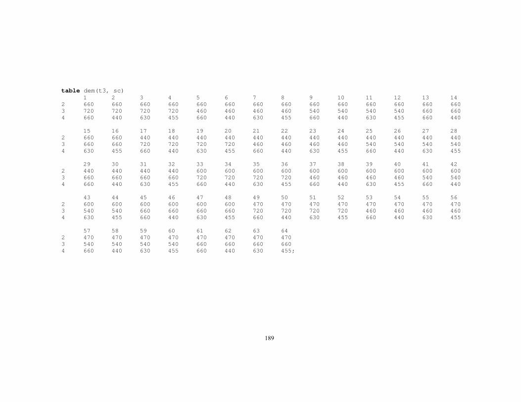
189

table dem(t3, sc) 1 2 3 4 5 6 7 8 9 10 11 12 13 14 2 660 660 660 660 660 660 660 660 660 660 660 660 660 660 3 720 720 720 720 460 460 460 460 540 540 540 540 660 660 4 660 440 630 455 660 440 630 455 660 440 630 455 660 440

15 16 17 18 19 20 21 22 23 24 25 26 27 28 2 660 660 440 440 440 440 440 440 440 440 440 440 440 440 3 660 660 720 720 720 720 460 460 460 460 540 540 540 540 4 630 455 660 440 630 455 660 440 630 455 660 440 630 455

29 30 31 32 33 34 35 36 37 38 39 40 41 42 2 440 440 440 440 600 600 600 600 600 600 600 600 600 600 3 660 660 660 660 720 720 720 720 460 460 460 460 540 540 4 660 440 630 455 660 440 630 455 660 440 630 455 660 440

43 44 45 46 47 48 49 50 51 52 53 54 55 56 2 600 600 600 600 600 600 470 470 470 470 470 470 470 470 3 540 540 660 660 660 660 720 720 720 720 460 460 460 460 4 630 455 660 440 630 455 660 440 630 455 660 440 630 455

57 58 59 60 61 62 63 64 2 470 470 470 470 470 470 470 470 3 540 540 540 540 660 660 660 660 4 660 440 630 455 660 440 630 455;

190

parameter prob(sc) /1 0.018 2 0.006 3 0.012 4 0.024 5 0.027 6 0.009 7 0.018 8 0.036 9 0.009 10 0.003 11 0.006 12 0.012 13 0.036 14 0.012 15 0.024 16 0.048

17 0.006 18 0.002 19 0.004 20 0.008 21 0.009 22 0.003 23 0.006 24 0.012 25 0.003 26 0.001 27 0.002 28 0.004 29 0.012 30 0.004 31 0.008 32 0.016

33 0.012 34 0.004 35 0.008 36 0.016 37 0.018 38 0.006 39 0.012 40 0.024 41 0.006 42 0.002 43 0.004 44 0.008 45 0.024 46 0.008 47 0.016 48 0.032

49 0.024 50 0.008 51 0.016 52 0.032 53 0.036 54 0.012 55 0.024 56 0.048 57 0.012 58 0.004 59 0.008 60 0.016 61 0.048 62 0.016 63 0.032 64 0.064/;

variables inv1(t) back1(t) invs1(t,sc) backs1(t,sc) f0(t) f1(t3) f0s(t,sc) f1s(t2,sc) zWCP zSUB zMASTER M;

positive variable inv1 back1 invs1 backs1 f0 f1 invs1 backs1 f0s f1s;

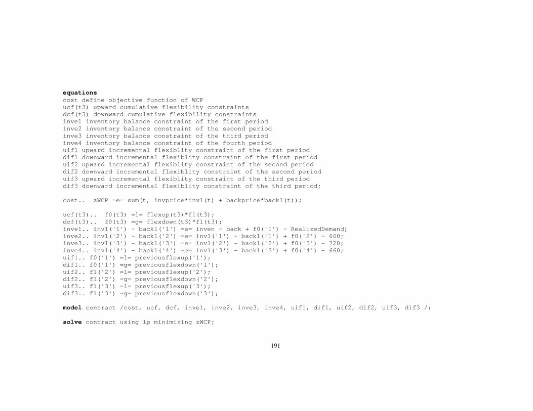
191

equations cost define objective function of WCP ucf(t3) upward cumulative flexibility constraints dcf(t3) downward cumulative flexibility constraints inve1 inventory balance constraint of the first period inve2 inventory balance constraint of the second period inve3 inventory balance constraint of the third period inve4 inventory balance constraint of the fourth period uif1 upward incremental flexiblity constraint of the first period dif1 downward incremental flexiblity constraint of the first period uif2 upward incremental flexiblity constraint of the second period dif2 downward incremental flexiblity constraint of the second period uif3 upward incremental flexiblity constraint of the third period dif3 downward incremental flexiblity constraint of the third period; cost.. zWCP =e= sum(t, invprice*inv1(t) + backprice*back1(t)); ucf(t3).. f0(t3) =l= flexup(t3)*f1(t3); dcf(t3).. f0(t3) =g= flexdown(t3)*f1(t3); inve1.. inv1('1') - back1('1') =e= inven - back + f0('1') - RealizedDemand; inve2.. inv1('2') - back1('2') =e= inv1('1') - back1('1') + f0('2') - 660; inve3.. inv1('3') - back1('3') =e= inv1('2') - back1('2') + f0('3') - 720; inve4.. inv1('4') - back1('4') =e= inv1('3') - back1('3') + f0('4') - 660; uif1.. f0('1') =l= previousflexup('1'); dif1.. f0('1') =g= previousflexdown('1'); uif2.. f1('2') =l= previousflexup('2'); dif2.. f1('2') =g= previousflexdown('2'); uif3.. f1('3') =l= previousflexup('3'); dif3.. f1('3') =g= previousflexdown('3'); model contract /cost, ucf, dcf, inve1, inve2, inve3, inve4, uif1, dif1, uif2, dif2, uif3, dif3 /; solve contract using lp minimizing zWCP;

192

equations cost2 define objective function of Sub Problem inves1(sc) inventory balance constraint of the first period inves2(sc) inventory balance constraint of the second period inves3(sc) inventory balance constraint of the third period inves4(sc) inventory balance constraint of the fourth period ucfs2(sc) upward cumulative flexibility constraint of the second period dcfs2(sc) downward cumulative flexibility constraint of the second period ucfs3(sc) upward cumulative flexibility constraint of the third period dcfs3(sc) downward cumulative flexibility constraint of the third period ucfs4(sc) upward cumulative flexibility constraint of the fourth period dcfs4(sc) downward cumulative flexibility constraint of the fourth period uifs1(sc) upward incremental flexiblity constraint of the first period difs1(sc) downward incremental flexiblity constraint of the first period nonantci11 nonanticipativity constraints for inventory carried of first period ... nonantci163 nonanticipativity constraints for inventory carried of first period nonantci21 nonanticipativity constraints for inventory carried of second period ... nonantci260 nonanticipativity constraints for inventory carried of second period nonantci31 nonanticipativity constraints for inventory carried of third period ... nonantci348 nonanticipativity constraints for inventory carried of third period nonantcb11 nonanticipativity constraints for amount backordered of first period ... nonantcb163 nonanticipativity constraints for amount backordered of first period nonantcb21 nonanticipativity constraints for amount backordered of second period ... nonantcb260 nonanticipativity constraints for amount backordered of second period nonantcb31 nonanticipativity constraints for amount backordered of third period ... nonantcb348 nonanticipativity constraints for amount backordered of third period; cost2.. zSUB =e= sum(sc, prob(sc)*sum(t, invprice*invs1(t, sc) + backprice*backs1(t, sc))); inves1(sc).. invs1('1', sc) - backs1('1', sc) =e= invens - backs + f0s('1', sc) - RealizedDemand;

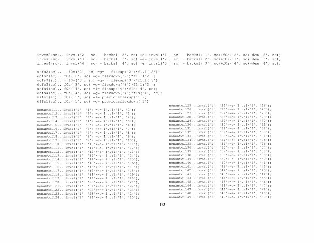
193

inves2(sc).. invs1('2', sc) - backs1('2', sc) =e= invs1('1', sc) - backs1('1', sc)+f0s('2', sc)-dem('2', sc); inves3(sc).. invs1('3', sc) - backs1('3', sc) =e= invs1('2', sc) - backs1('2', sc)+f0s('3', sc)-dem('3', sc); inves4(sc).. invs1('4', sc) - backs1('4', sc) =e= invs1('3', sc) - backs1('3', sc)+f0s('4', sc)-dem('4', sc); ucfs2(sc).. - f0s('2', sc) =g= - flexup('2')*f1.l('2'); dcfs2(sc).. f0s('2', sc) =g= flexdown('2')*f1.l('2'); ucfs3(sc).. - f0s('3', sc) =g= - flexup('3')*f1.l('3'); dcfs3(sc).. f0s('3', sc) =g= flexdown('3')*f1.l('3'); ucfs4(sc).. f0s('4', sc) =l= flexup('4')*f1s('4', sc); dcfs4(sc).. f0s('4', sc) =g= flexdown('4')*f1s('4', sc); uifs1(sc).. f0s('1', sc) =l= previousflexup('1'); difs1(sc).. f0s('1', sc) =g= previousflexdown('1'); nonantci11.. invs1('1', '1') =e= invs1('1', '2'); nonantci12.. invs1('1', '2') =e= invs1('1', '3'); nonantci13.. invs1('1', '3') =e= invs1('1', '4'); nonantci14.. invs1('1', '4') =e= invs1('1', '5'); nonantci15.. invs1('1', '5') =e= invs1('1', '6'); nonantci16.. invs1('1', '6') =e= invs1('1', '7'); nonantci17.. invs1('1', '7') =e= invs1('1', '8'); nonantci18.. invs1('1', '8') =e= invs1('1', '9'); nonantci19.. invs1('1', '9') =e= invs1('1', '10'); nonantci110.. invs1('1', '10')=e= invs1('1', '11'); nonantci111.. invs1('1', '11')=e= invs1('1', '12'); nonantci112.. invs1('1', '12')=e= invs1('1', '13'); nonantci113.. invs1('1', '13')=e= invs1('1', '14'); nonantci114.. invs1('1', '14')=e= invs1('1', '15'); nonantci115.. invs1('1', '15')=e= invs1('1', '16'); nonantci116.. invs1('1', '16')=e= invs1('1', '17'); nonantci117.. invs1('1', '17')=e= invs1('1', '18'); nonantci118.. invs1('1', '18')=e= invs1('1', '19'); nonantci119.. invs1('1', '19')=e= invs1('1', '20'); nonantci120.. invs1('1', '20')=e= invs1('1', '21'); nonantci121.. invs1('1', '21')=e= invs1('1', '22'); nonantci122.. invs1('1', '22')=e= invs1('1', '23'); nonantci123.. invs1('1', '23')=e= invs1('1', '24'); nonantci124.. invs1('1', '24')=e= invs1('1', '25');

nonantci125.. invs1('1', '25')=e= invs1('1', '26'); nonantci126.. invs1('1', '26')=e= invs1('1', '27'); nonantci127.. invs1('1', '27')=e= invs1('1', '28'); nonantci128.. invs1('1', '28')=e= invs1('1', '29'); nonantci129.. invs1('1', '29')=e= invs1('1', '30'); nonantci130.. invs1('1', '30')=e= invs1('1', '31'); nonantci131.. invs1('1', '31')=e= invs1('1', '32'); nonantci132.. invs1('1', '32')=e= invs1('1', '33'); nonantci133.. invs1('1', '33')=e= invs1('1', '34'); nonantci134.. invs1('1', '34')=e= invs1('1', '35'); nonantci135.. invs1('1', '35')=e= invs1('1', '36'); nonantci136.. invs1('1', '36')=e= invs1('1', '37'); nonantci137.. invs1('1', '37')=e= invs1('1', '38'); nonantci138.. invs1('1', '38')=e= invs1('1', '39'); nonantci139.. invs1('1', '39')=e= invs1('1', '40'); nonantci140.. invs1('1', '40')=e= invs1('1', '41'); nonantci141.. invs1('1', '41')=e= invs1('1', '42'); nonantci142.. invs1('1', '42')=e= invs1('1', '43'); nonantci143.. invs1('1', '43')=e= invs1('1', '44'); nonantci144.. invs1('1', '44')=e= invs1('1', '45'); nonantci145.. invs1('1', '45')=e= invs1('1', '46'); nonantci146.. invs1('1', '46')=e= invs1('1', '47'); nonantci147.. invs1('1', '47')=e= invs1('1', '48'); nonantci148.. invs1('1', '48')=e= invs1('1', '49'); nonantci149.. invs1('1', '49')=e= invs1('1', '50');

194

nonantci150.. invs1('1', '50')=e= invs1('1', '51'); nonantci151.. invs1('1', '51')=e= invs1('1', '52'); nonantci152.. invs1('1', '52')=e= invs1('1', '53'); nonantci153.. invs1('1', '53')=e= invs1('1', '54'); nonantci154.. invs1('1', '54')=e= invs1('1', '55'); nonantci155.. invs1('1', '55')=e= invs1('1', '56'); nonantci156.. invs1('1', '56')=e= invs1('1', '57'); nonantci157.. invs1('1', '57')=e= invs1('1', '58'); nonantci158.. invs1('1', '58')=e= invs1('1', '59'); nonantci159.. invs1('1', '59')=e= invs1('1', '60'); nonantci160.. invs1('1', '60')=e= invs1('1', '61'); nonantci161.. invs1('1', '61')=e= invs1('1', '62'); nonantci162.. invs1('1', '62')=e= invs1('1', '63'); nonantci163.. invs1('1', '63')=e= invs1('1', '64'); nonantci21.. invs1('2', '1') =e= invs1('2', '2'); nonantci22.. invs1('2', '2') =e= invs1('2', '3'); nonantci23.. invs1('2', '3') =e= invs1('2', '4'); nonantci24.. invs1('2', '4') =e= invs1('2', '5'); nonantci25.. invs1('2', '5') =e= invs1('2', '6'); nonantci26.. invs1('2', '6') =e= invs1('2', '7'); nonantci27.. invs1('2', '7') =e= invs1('2', '8'); nonantci28.. invs1('2', '8') =e= invs1('2', '9'); nonantci29.. invs1('2', '9') =e= invs1('2', '10'); nonantci210.. invs1('2', '10')=e= invs1('2', '11'); nonantci211.. invs1('2', '11')=e= invs1('2', '12'); nonantci212.. invs1('2', '12')=e= invs1('2', '13'); nonantci213.. invs1('2', '13')=e= invs1('2', '14'); nonantci214.. invs1('2', '14')=e= invs1('2', '15'); nonantci215.. invs1('2', '15')=e= invs1('2', '16'); nonantci216.. invs1('2', '17')=e= invs1('2', '18'); nonantci217.. invs1('2', '18')=e= invs1('2', '19'); nonantci218.. invs1('2', '19')=e= invs1('2', '20'); nonantci219.. invs1('2', '20')=e= invs1('2', '21'); nonantci220.. invs1('2', '21')=e= invs1('2', '22'); nonantci221.. invs1('2', '22')=e= invs1('2', '23'); nonantci222.. invs1('2', '23')=e= invs1('2', '24'); nonantci223.. invs1('2', '24')=e= invs1('2', '25'); nonantci224.. invs1('2', '25')=e= invs1('2', '26'); nonantci225.. invs1('2', '26')=e= invs1('2', '27');

nonantci226.. invs1('2', '27')=e= invs1('2', '28'); nonantci227.. invs1('2', '28')=e= invs1('2', '29'); nonantci228.. invs1('2', '29')=e= invs1('2', '30'); nonantci229.. invs1('2', '30')=e= invs1('2', '31'); nonantci230.. invs1('2', '31')=e= invs1('2', '32'); nonantci231.. invs1('2', '33')=e= invs1('2', '34'); nonantci232.. invs1('2', '34')=e= invs1('2', '35'); nonantci233.. invs1('2', '35')=e= invs1('2', '36'); nonantci234.. invs1('2', '36')=e= invs1('2', '37'); nonantci235.. invs1('2', '37')=e= invs1('2', '38'); nonantci236.. invs1('2', '38')=e= invs1('2', '39'); nonantci237.. invs1('2', '39')=e= invs1('2', '40'); nonantci238.. invs1('2', '40')=e= invs1('2', '41'); nonantci239.. invs1('2', '41')=e= invs1('2', '42'); nonantci240.. invs1('2', '42')=e= invs1('2', '43'); nonantci241.. invs1('2', '43')=e= invs1('2', '44'); nonantci242.. invs1('2', '44')=e= invs1('2', '45'); nonantci243.. invs1('2', '45')=e= invs1('2', '46'); nonantci244.. invs1('2', '46')=e= invs1('2', '47'); nonantci245.. invs1('2', '47')=e= invs1('2', '48'); nonantci246.. invs1('2', '49')=e= invs1('2', '50'); nonantci247.. invs1('2', '50')=e= invs1('2', '51'); nonantci248.. invs1('2', '51')=e= invs1('2', '52'); nonantci249.. invs1('2', '52')=e= invs1('2', '53'); nonantci250.. invs1('2', '53')=e= invs1('2', '54'); nonantci251.. invs1('2', '54')=e= invs1('2', '55'); nonantci252.. invs1('2', '55')=e= invs1('2', '56'); nonantci253.. invs1('2', '56')=e= invs1('2', '57'); nonantci254.. invs1('2', '57')=e= invs1('2', '58'); nonantci255.. invs1('2', '58')=e= invs1('2', '59'); nonantci256.. invs1('2', '59')=e= invs1('2', '60'); nonantci257.. invs1('2', '60')=e= invs1('2', '61'); nonantci258.. invs1('2', '61')=e= invs1('2', '62'); nonantci259.. invs1('2', '62')=e= invs1('2', '63'); nonantci260.. invs1('2', '63')=e= invs1('2', '64'); nonantci31.. invs1('3', '1') =e= invs1('3', '2'); nonantci32.. invs1('3', '2') =e= invs1('3', '3'); nonantci33.. invs1('3', '3') =e= invs1('3', '4'); nonantci34.. invs1('3', '5') =e= invs1('3', '6');

195

nonantci35.. invs1('3', '6') =e= invs1('3', '7'); nonantci36.. invs1('3', '7') =e= invs1('3', '8'); nonantci37.. invs1('3', '9') =e= invs1('3', '10'); nonantci38.. invs1('3', '10') =e= invs1('3', '11'); nonantci39.. invs1('3', '11') =e= invs1('3', '12'); nonantci310.. invs1('3', '13')=e= invs1('3', '14'); nonantci311.. invs1('3', '14')=e= invs1('3', '15'); nonantci312.. invs1('3', '15')=e= invs1('3', '16'); nonantci313.. invs1('3', '17')=e= invs1('3', '18'); nonantci314.. invs1('3', '18')=e= invs1('3', '19'); nonantci315.. invs1('3', '19')=e= invs1('3', '20'); nonantci316.. invs1('3', '21')=e= invs1('3', '22'); nonantci317.. invs1('3', '22')=e= invs1('3', '23'); nonantci318.. invs1('3', '23')=e= invs1('3', '24'); nonantci319.. invs1('3', '25')=e= invs1('3', '26'); nonantci320.. invs1('3', '26')=e= invs1('3', '27'); nonantci321.. invs1('3', '27')=e= invs1('3', '28'); nonantci322.. invs1('3', '29')=e= invs1('3', '30'); nonantci323.. invs1('3', '30')=e= invs1('3', '31'); nonantci324.. invs1('3', '31')=e= invs1('3', '32'); nonantci325.. invs1('3', '33')=e= invs1('3', '34'); nonantci326.. invs1('3', '34')=e= invs1('3', '35'); nonantci327.. invs1('3', '35')=e= invs1('3', '36'); nonantci328.. invs1('3', '37')=e= invs1('3', '38'); nonantci329.. invs1('3', '38')=e= invs1('3', '39'); nonantci330.. invs1('3', '39')=e= invs1('3', '40'); nonantci331.. invs1('3', '41')=e= invs1('3', '42'); nonantci332.. invs1('3', '42')=e= invs1('3', '43'); nonantci333.. invs1('3', '43')=e= invs1('3', '44'); nonantci334.. invs1('3', '45')=e= invs1('3', '46'); nonantci335.. invs1('3', '46')=e= invs1('3', '47'); nonantci336.. invs1('3', '47')=e= invs1('3', '48'); nonantci337.. invs1('3', '49')=e= invs1('3', '50'); nonantci338.. invs1('3', '50')=e= invs1('3', '51'); nonantci339.. invs1('3', '51')=e= invs1('3', '52'); nonantci340.. invs1('3', '53')=e= invs1('3', '54'); nonantci341.. invs1('3', '54')=e= invs1('3', '55'); nonantci342.. invs1('3', '55')=e= invs1('3', '56'); nonantci343.. invs1('3', '57')=e= invs1('3', '58');

nonantci344.. invs1('3', '58')=e= invs1('3', '59'); nonantci345.. invs1('3', '59')=e= invs1('3', '60'); nonantci346.. invs1('3', '61')=e= invs1('3', '62'); nonantci347.. invs1('3', '62')=e= invs1('3', '63'); nonantci348.. invs1('3', '63')=e= invs1('3', '64'); nonantcb11.. backs1('1', '1') =e= backs1('1', '2'); nonantcb12.. backs1('1', '2') =e= backs1('1', '3'); nonantcb13.. backs1('1', '3') =e= backs1('1', '4'); nonantcb14.. backs1('1', '4') =e= backs1('1', '5'); nonantcb15.. backs1('1', '5') =e= backs1('1', '6'); nonantcb16.. backs1('1', '6') =e= backs1('1', '7'); nonantcb17.. backs1('1', '7') =e= backs1('1', '8'); nonantcb18.. backs1('1', '8') =e= backs1('1', '9'); nonantcb19.. backs1('1', '9')=e= backs1('1', '10'); nonantcb110.. backs1('1', '10')=e=backs1('1','11'); nonantcb111.. backs1('1', '11')=e=backs1('1','12'); nonantcb112.. backs1('1', '12')=e=backs1('1','13'); nonantcb113.. backs1('1', '13')=e=backs1('1','14'); nonantcb114.. backs1('1', '14')=e=backs1('1','15'); nonantcb115.. backs1('1', '15')=e=backs1('1','16'); nonantcb116.. backs1('1', '16')=e=backs1('1','17'); nonantcb117.. backs1('1', '17')=e=backs1('1','18'); nonantcb118.. backs1('1', '18')=e=backs1('1','19'); nonantcb119.. backs1('1', '19')=e=backs1('1','20'); nonantcb120.. backs1('1', '20')=e=backs1('1','21'); nonantcb121.. backs1('1', '21')=e=backs1('1','22'); nonantcb122.. backs1('1', '22')=e=backs1('1','23'); nonantcb123.. backs1('1', '23')=e=backs1('1','24'); nonantcb124.. backs1('1', '24')=e=backs1('1','25'); nonantcb125.. backs1('1', '25')=e=backs1('1','26'); nonantcb126.. backs1('1', '26')=e=backs1('1','27'); nonantcb127.. backs1('1', '27')=e=backs1('1','28'); nonantcb128.. backs1('1', '28')=e=backs1('1','29'); nonantcb129.. backs1('1', '29')=e=backs1('1','30'); nonantcb130.. backs1('1', '30')=e=backs1('1','31'); nonantcb131.. backs1('1', '31')=e=backs1('1','32'); nonantcb132.. backs1('1', '32')=e=backs1('1','33'); nonantcb133.. backs1('1', '33')=e=backs1('1','34'); nonantcb134.. backs1('1', '34')=e=backs1('1','35');

196

nonantcb135.. backs1('1', '35')=e=backs1('1','36'); nonantcb136.. backs1('1', '36')=e=backs1('1','37'); nonantcb137.. backs1('1', '37')=e=backs1('1','38'); nonantcb138.. backs1('1', '38')=e=backs1('1','39'); nonantcb139.. backs1('1', '39')=e=backs1('1','40'); nonantcb140.. backs1('1', '40')=e=backs1('1','41'); nonantcb141.. backs1('1', '41')=e=backs1('1','42'); nonantcb142.. backs1('1', '42')=e=backs1('1','43'); nonantcb143.. backs1('1', '43')=e=backs1('1','44'); nonantcb144.. backs1('1', '44')=e=backs1('1','45'); nonantcb145.. backs1('1', '45')=e=backs1('1','46'); nonantcb146.. backs1('1', '46')=e=backs1('1','47'); nonantcb147.. backs1('1', '47')=e=backs1('1','48'); nonantcb148.. backs1('1', '48')=e=backs1('1','49'); nonantcb149.. backs1('1', '49')=e=backs1('1','50'); nonantcb150.. backs1('1', '50')=e=backs1('1','51'); nonantcb151.. backs1('1', '51')=e=backs1('1','52'); nonantcb152.. backs1('1', '52')=e=backs1('1','53'); nonantcb153.. backs1('1', '53')=e=backs1('1','54'); nonantcb154.. backs1('1', '54')=e=backs1('1','55'); nonantcb155.. backs1('1', '55')=e=backs1('1','56'); nonantcb156.. backs1('1', '56')=e=backs1('1','57'); nonantcb157.. backs1('1', '57')=e=backs1('1','58'); nonantcb158.. backs1('1', '58')=e=backs1('1','59'); nonantcb159.. backs1('1', '59')=e=backs1('1','60'); nonantcb160.. backs1('1', '60')=e=backs1('1','61'); nonantcb161.. backs1('1', '61')=e=backs1('1','62'); nonantcb162.. backs1('1', '62')=e=backs1('1','63'); nonantcb163.. backs1('1', '63')=e=backs1('1','64'); nonantcb21.. backs1('2', '1') =e= backs1('2', '2'); nonantcb22.. backs1('2', '2') =e= backs1('2', '3'); nonantcb23.. backs1('2', '3') =e= backs1('2', '4'); nonantcb24.. backs1('2', '4') =e= backs1('2', '5'); nonantcb25.. backs1('2', '5') =e= backs1('2', '6'); nonantcb26.. backs1('2', '6') =e= backs1('2', '7'); nonantcb27.. backs1('2', '7') =e= backs1('2', '8'); nonantcb28.. backs1('2', '8') =e= backs1('2', '9'); nonantcb29.. backs1('2', '9') =e= backs1('2','10'); nonantcb210.. backs1('2', '10')=e= backs1('2',11');

nonantcb211.. backs1('2', '11')=e=backs1('2','12'); nonantcb212.. backs1('2', '12')=e=backs1('2','13'); nonantcb213.. backs1('2', '13')=e=backs1('2','14'); nonantcb214.. backs1('2', '14')=e=backs1('2','15'); nonantcb215.. backs1('2', '15')=e=backs1('2','16'); nonantcb216.. backs1('2', '17')=e=backs1('2','18'); nonantcb217.. backs1('2', '18')=e=backs1('2','19'); nonantcb218.. backs1('2', '19')=e=backs1('2','20'); nonantcb219.. backs1('2', '20')=e=backs1('2','21'); nonantcb220.. backs1('2', '21')=e=backs1('2','22'); nonantcb221.. backs1('2', '22')=e=backs1('2','23'); nonantcb222.. backs1('2', '23')=e=backs1('2','24'); nonantcb223.. backs1('2', '24')=e=backs1('2','25'); nonantcb224.. backs1('2', '25')=e=backs1('2','26'); nonantcb225.. backs1('2', '26')=e=backs1('2','27'); nonantcb226.. backs1('2', '27')=e=backs1('2','28'); nonantcb227.. backs1('2', '28')=e=backs1('2','29'); nonantcb228.. backs1('2', '29')=e=backs1('2','30'); nonantcb229.. backs1('2', '30')=e=backs1('2','31'); nonantcb230.. backs1('2', '31')=e=backs1('2','32'); nonantcb231.. backs1('2', '33')=e=backs1('2','34'); nonantcb232.. backs1('2', '34')=e=backs1('2','35'); nonantcb233.. backs1('2', '35')=e=backs1('2','36'); nonantcb234.. backs1('2', '36')=e=backs1('2','37'); nonantcb235.. backs1('2', '37')=e=backs1('2','38'); nonantcb236.. backs1('2', '38')=e=backs1('2','39'); nonantcb237.. backs1('2', '39')=e=backs1('2','40'); nonantcb238.. backs1('2', '40')=e=backs1('2','41'); nonantcb239.. backs1('2', '41')=e=backs1('2','42'); nonantcb240.. backs1('2', '42')=e=backs1('2','43'); nonantcb241.. backs1('2', '43')=e=backs1('2','44'); nonantcb242.. backs1('2', '44')=e=backs1('2','45'); nonantcb243.. backs1('2', '45')=e=backs1('2','46'); nonantcb244.. backs1('2', '46')=e=backs1('2','47'); nonantcb245.. backs1('2', '47')=e=backs1('2','48'); nonantcb246.. backs1('2', '49')=e=backs1('2','50'); nonantcb247.. backs1('2', '50')=e=backs1('2','51'); nonantcb248.. backs1('2', '51')=e=backs1('2','52'); nonantcb249.. backs1('2', '52')=e=backs1('2','53');

197

nonantcb250.. backs1('2', '53')=e=backs1('2','54'); nonantcb251.. backs1('2', '54')=e=backs1('2','55'); nonantcb252.. backs1('2', '55')=e=backs1('2','56'); nonantcb253.. backs1('2', '56')=e=backs1('2','57'); nonantcb254.. backs1('2', '57')=e=backs1('2','58'); nonantcb255.. backs1('2', '58')=e=backs1('2','59'); nonantcb256.. backs1('2', '59')=e=backs1('2','60'); nonantcb257.. backs1('2', '60')=e=backs1('2','61'); nonantcb258.. backs1('2', '61')=e=backs1('2','62'); nonantcb259.. backs1('2', '62')=e=backs1('2','63'); nonantcb260.. backs1('2', '63')=e=backs1('2','64'); nonantcb31.. backs1('3', '1') =e= backs1('3', '2'); nonantcb32.. backs1('3', '2') =e= backs1('3', '3'); nonantcb33.. backs1('3', '3') =e= backs1('3', '4'); nonantcb34.. backs1('3', '5') =e= backs1('3', '6'); nonantcb35.. backs1('3', '6') =e= backs1('3', '7'); nonantcb36.. backs1('3', '7') =e= backs1('3', '8'); nonantcb37.. backs1('3', '9') =e= backs1('3','10'); nonantcb38.. backs1('3', '10') =e=backs1('3','11'); nonantcb39.. backs1('3', '11')=e=backs1('3', '12'); nonantcb310.. backs1('3', '13')=e=backs1('3','14'); nonantcb311.. backs1('3', '14')=e=backs1('3','15'); nonantcb312.. backs1('3', '15')=e=backs1('3','16'); nonantcb313.. backs1('3', '17')=e=backs1('3','18'); nonantcb314.. backs1('3', '18')=e=backs1('3','19'); nonantcb315.. backs1('3', '19')=e=backs1('3','20'); nonantcb316.. backs1('3', '21')=e=backs1('3','22'); nonantcb317.. backs1('3', '22')=e=backs1('3','23'); nonantcb318.. backs1('3', '23')=e=backs1('3','24'); nonantcb319.. backs1('3', '25')=e=backs1('3','26'); nonantcb320.. backs1('3', '26')=e=backs1('3','27'); nonantcb321.. backs1('3', '27')=e=backs1('3','28'); nonantcb322.. backs1('3', '29')=e=backs1('3','30'); nonantcb323.. backs1('3', '30')=e=backs1('3','31'); nonantcb324.. backs1('3', '31')=e=backs1('3','32'); nonantcb325.. backs1('3', '33')=e=backs1('3','34'); nonantcb326.. backs1('3', '34')=e=backs1('3','35'); nonantcb327.. backs1('3', '35')=e=backs1('3','36'); nonantcb328.. backs1('3', '37')=e=backs1('3','38');

nonantcb329.. backs1('3', '38')=e=backs1('3','39'); nonantcb330.. backs1('3', '39')=e=backs1('3','40'); nonantcb331.. backs1('3', '41')=e=backs1('3','42'); nonantcb332.. backs1('3', '42')=e=backs1('3','43'); nonantcb333.. backs1('3', '43')=e=backs1('3','44'); nonantcb334.. backs1('3', '45')=e=backs1('3','46'); nonantcb335.. backs1('3', '46')=e=backs1('3','47'); nonantcb336.. backs1('3', '47')=e=backs1('3','48'); nonantcb337.. backs1('3', '49')=e=backs1('3','50'); nonantcb338.. backs1('3', '50')=e=backs1('3','51'); nonantcb339.. backs1('3', '51')=e=backs1('3','52'); nonantcb340.. backs1('3', '53')=e=backs1('3','54'); nonantcb341.. backs1('3', '54')=e=backs1('3','55'); nonantcb342.. backs1('3', '55')=e=backs1('3','56'); nonantcb343.. backs1('3', '57')=e=backs1('3','58'); nonantcb344.. backs1('3', '58')=e=backs1('3','59'); nonantcb345.. backs1('3', '59')=e=backs1('3','60'); nonantcb346.. backs1('3', '61')=e=backs1('3','62'); nonantcb347.. backs1('3', '62')=e=backs1('3','63'); nonantcb348.. backs1('3', '63')=e=backs1('3','64'); model sub /cost2, inves1, inves2, inves3, inves4, ucfs2, dcfs2, ucfs3, dcfs3, ucfs4, dcfs4, uifs1, difs1, nonantci11, nonantci12, nonantci13, nonantci14, nonantci15, nonantci16, nonantci17, nonantci18, nonantci19, nonantci110, nonantci111, nonantci112, nonantci113, nonantci114, nonantci115, nonantci116, nonantci117, nonantci118, nonantci119, nonantci120, nonantci121, nonantci122, nonantci123, nonantci124, nonantci125, nonantci126, nonantci127, nonantci128, nonantci129, nonantci130, nonantci131, nonantci132, nonantci133, nonantci134, nonantci135, nonantci136, nonantci137, nonantci138, nonantci139, nonantci140, nonantci141, nonantci142, nonantci143, nonantci144, nonantci145, nonantci146, nonantci147, nonantci148, nonantci149, nonantci150, nonantci151, nonantci152, nonantci153, nonantci154, nonantci155, nonantci156, nonantci157, nonantci158, nonantci159, nonantci160, nonantci161, nonantci162, nonantci163, nonantci21,

198

nonantci22, nonantci23, nonantci24, nonantci25, nonantci26, nonantci27, nonantci28, nonantci29, nonantci210, nonantci211, nonantci212, nonantci213, nonantci214, nonantci215, nonantci216, nonantci217, nonantci218, nonantci219, nonantci220, nonantci221, nonantci222, nonantci223, nonantci224, nonantci225, nonantci226, nonantci227, nonantci228, nonantci229, nonantci230, nonantci231, nonantci232, nonantci233, nonantci234, nonantci235, nonantci236, nonantci237, nonantci238, nonantci239, nonantci240,nonantci241, nonantci242, nonantci243, nonantci244, nonantci245, nonantci246, nonantci247, nonantci248, nonantci249, nonantci250, nonantci251, nonantci252, nonantci253, nonantci254, nonantci255, nonantci256, nonantci257, nonantci258, nonantci259, nonantci260, nonantci31, nonantci32, nonantci33, nonantci34, nonantci35, nonantci36, nonantci37, nonantci38, nonantci39, nonantci310, nonantci311, nonantci312, nonantci313, nonantci314, nonantci315, nonantci316, nonantci317, nonantci318, nonantci319, nonantci320, nonantci321, nonantci322, nonantci323, nonantci324, nonantci325, nonantci326, nonantci327, nonantci328, nonantci329, nonantci330, nonantci331, nonantci332, nonantci333, nonantci334, nonantci335, nonantci336, nonantci337, nonantci338, nonantci339, nonantci340, nonantci341, nonantci342, nonantci343, nonantci344, nonantci345, nonantci346, nonantci347, nonantci348, nonantcb11, nonantcb12, nonantcb13, nonantcb14, nonantcb15, nonantcb16, nonantcb17, nonantcb18, nonantcb19, nonantcb110, nonantcb111, nonantcb112, nonantcb113, nonantcb114, nonantcb115, nonantcb116, nonantcb117, nonantcb118, nonantcb119, nonantcb120, nonantcb121, nonantcb122, nonantcb123, nonantcb124, nonantcb125, nonantcb126, nonantcb127, nonantcb128, nonantcb129, nonantcb130, nonantcb131, nonantcb132, nonantcb133, nonantcb134, nonantcb135, nonantcb136, nonantcb137, nonantcb138, nonantcb139, nonantcb140, nonantcb141, nonantcb142, nonantcb143, nonantcb144, nonantcb145, nonantcb146, nonantcb147, nonantcb148,

nonantcb149, nonantcb150, nonantcb151, nonantcb152, nonantcb153, nonantcb154, nonantcb155, nonantcb156, nonantcb157, nonantcb158, nonantcb159, nonantcb160, nonantcb161, nonantcb162, nonantcb163, nonantcb21, nonantcb22, nonantcb23, nonantcb24, nonantcb25, nonantcb26, nonantcb27, nonantcb28, nonantcb29, nonantcb210, nonantcb211, nonantcb212, nonantcb213, nonantcb214, nonantcb215, nonantcb216, nonantcb217, nonantcb218, nonantcb219, nonantcb220, nonantcb221, nonantcb222, nonantcb223, nonantcb224, nonantcb225, nonantcb226, nonantcb227, nonantcb228, nonantcb229, nonantcb230, nonantcb231, nonantcb232, nonantcb233, nonantcb234, nonantcb235, nonantcb236, nonantcb237, nonantcb238, nonantcb239, nonantcb240, nonantcb241, nonantcb242, nonantcb243, nonantcb244, nonantcb245, nonantcb246, nonantcb247, nonantcb248, nonantcb249, nonantcb250, nonantcb251, nonantcb252, nonantcb253, nonantcb254, nonantcb255, nonantcb256, nonantcb257, nonantcb258, nonantcb259, nonantcb260, nonantcb31, nonantcb32, nonantcb33, nonantcb34, nonantcb35, nonantcb36, nonantcb37, nonantcb38, nonantcb39, nonantcb310, nonantcb311, nonantcb312, nonantcb313, nonantcb314, nonantcb315, nonantcb316, nonantcb317, nonantcb318, nonantcb319, nonantcb320, nonantcb321, nonantcb322, nonantcb323, nonantcb324, nonantcb325, nonantcb326, nonantcb327, nonantcb328, nonantcb329, nonantcb330, nonantcb331, nonantcb332, nonantcb333, nonantcb334, nonantcb335, nonantcb336, nonantcb337, nonantcb338, nonantcb339, nonantcb340, nonantcb341, nonantcb342, nonantcb343, nonantcb344, nonantcb345, nonantcb346, nonantcb347, nonantcb348 /;

199

set ss / 1*20/ s(ss); parameter rep(ss, *) pinvs1(t, sc, ss) pbacks1(t, sc, ss) dualucfs2(sc, ss) dualdcfs2(sc, ss) dualucfs3(sc, ss) dualdcfs3(sc, ss) lastff0(*, sc) ff0(*, sc, ss); equations cost3 define objective function of Master Problem uifmaster2 upward incremental flexibility of the second period difmaster2 downward incremental flexibility of the second period uifmaster3 upward incremental flexibility of the third period difmaster3 downward incremental flexibility of the third period benderscuts(ss) Bender's CUT fc1(sc) Feasibility constraints fc2(sc) Feasibility constraints fc3(sc) Feasibility constraints fc4(sc) Feasibility constraints; cost3.. zMASTER =e= M; uifmaster2.. f1('2') =l= previousflexup('2'); difmaster2.. f1('2') =g= previousflexdown('2'); uifmaster3.. f1('3') =l= previousflexup('3'); difmaster3.. f1('3') =g= previousflexdown('3'); fc1(sc).. lastff0('2', sc) =l= flexup('2')*f1('2'); fc2(sc).. lastff0('2', sc) =g= flexdown('2')*f1('2');

200

fc3(sc).. lastff0('3', sc) =l= flexup('3')*f1('3'); fc4(sc).. lastff0('3', sc) =g= flexdown('3')*f1('3'); benderscuts(s).. M =g= sum(sc, prob(sc)*(sum(t, invprice*pinvs1(t, sc, s) + backprice*pbacks1(t, sc, s)))) + sum(sc, dualucfs2(sc, s)*( - flexup('2')*f1('2') + ff0('2',sc, s))) + sum(sc, dualdcfs2(sc, s)*(flexdown('2')*f1('2') - ff0('2', sc, s))) + sum(sc, dualucfs3(sc, s)*(- flexup('3')*f1('3') + ff0('3',sc, s))) + sum(sc, dualdcfs3(sc, s)*(flexdown('3')*f1('3') - ff0('3', sc, s))); model master /cost3, uifmaster2, difmaster2, uifmaster3, difmaster3, fc1, fc2, fc3, fc4, benderscuts/; rep('1', 'gap') = inf; rep('1', 'lb') = -inf; rep('1', 'ub') = inf; loop (ss$(rep(ss, 'gap') > 0.01 ), solve sub using lp minimizing zSUB; rep(ss + 1, 'subopt') = zSUB.l; rep(ss + 1, 'ub') = min(rep(ss, 'ub'), rep(ss + 1, 'subopt')); s(ss) = ord(ss); pinvs1(t, sc, ss) = invs1.l(t, sc); pbacks1(t, sc, ss) = backs1.l(t, sc); dualucfs2(sc, ss) = ucfs2.m(sc); dualdcfs2(sc, ss) = dcfs2.m(sc); dualucfs3(sc, ss) = ucfs3.m(sc); dualdcfs3(sc, ss) = dcfs3.m(sc); ff0('2', sc, ss) = f0s.l('2', sc); ff0('3', sc, ss) = f0s.l('3', sc); lastff0('2', sc ) = f0s.l('2', sc); lastff0('3', sc ) = f0s.l('3', sc); solve master using lp minimizing zMASTER; rep(ss + 1, 'mastopt') = zMASTER.l; rep(ss + 1, 'lb') = rep(ss + 1, 'mastopt'); rep(ss + 1, 'gap') = rep(ss + 1, 'ub') - rep(ss + 1, 'lb'); ); display M.l, inv1.l, back1.l, invs1.l, backs1.l, f0s.l, f1.l, p, rep;

201

APPENDIX E

AVERAGE COSTS OF THE SUPPLY CHAIN ACTORS IN

DECENTRALIZED ENVIRONMENT IN THE SECOND CASE

Table E.1 Average Costs of the SC Actors in the Decentralized Environment in Medium DEVAR

DEVAR: Medium/High ; FLEX: Tight/Loose ; COST: Low/High DECENTRALIZED ENVIRONMENT

DEVAR (FB2, FM) / (CB, CM) 1st Buyer 2nd Buyer Manufacturer Total (T.T) / (L.L) 0.0 213.9 2442.9 2656.8 (T.T) / (L.H) 0.0 213.9 4556.5 4770.4 (T.T) / (H.L) 0.2 305.6 2479.4 2785.2 (T.T) / (H.H) 0.2 305.6 4629.8 4935.6 (T.L) / (L.L) 0.0 213.9 2441.0 2654.9 (T.L) / (L.H) 0.0 213.9 4553.5 4767.4 (T.L) / (H.L) 0.2 305.6 2477.5 2783.3 (T.L) / (H.H) 0.2 305.6 4626.8 4932.6 (L.T) / (L.L) 0.0 92.8 2386.5 2479.3 (L.T) / (L.H) 0.0 92.8 4397.1 4489.9 (L.T) / (H.L) 0.2 92.8 2408.9 2501.9 (L.T) / (H.H) 0.2 92.8 4437.8 4530.8 (L.L) / (L.L) 0.0 92.8 2384.8 2477.6 (L.L) / (L.H) 0.0 92.8 4394.5 4487.3 (L.L) / (H.L) 0.2 92.8 2407.3 2500.3

MED

IUM

DEV

AR

(L.L) / (H.H) 0.2 92.8 4435.2 4528.2

202

Table E.2 Average Costs of the SC Actors in the Decentralized Environment in High DEVAR

DEVAR: Medium/High ; FLEX: Tight/Loose ; COST: Low/High DECENTRALIZED ENVIRONMENT

DEVAR (FB2. FM) / (CB. CM) 1st

Buyer 2nd Buyer Manufacturer Total (T.T) / (L.L) 130.6 164.7 3172.0 3467.3 (T.T) / (L.H) 130.6 164.7 5790.4 6085.7 (T.T) / (H.L) 130.9 265.6 3294.8 3691.2 (T.T) / (H.H) 130.9 265.6 6013.4 6409.9 (T.L) / (L.L) 130.6 164.7 3169.5 3464.8 (T.L) / (L.H) 130.6 164.7 5787.4 6082.7 (T.L) / (H.L) 130.9 265.6 3292.3 3688.8 (T.L) / (H.H) 130.9 265.6 6010.3 6406.7 (L.T) / (L.L) 130.6 100.1 3157.8 3388.4 (L.T) / (L.H) 130.6 100.1 5745.0 5975.7 (L.T) / (H.L) 130.9 96.4 3192.0 3419.3 (L.T) / (H.H) 130.9 96.4 5806.0 6033.2 (L.L) / (L.L) 130.6 100.1 3155.5 3386.2 (L.L) / (L.H) 130.6 100.1 5742.1 5972.7 (L.L) / (H.L) 130.9 96.4 3189.9 3417.1

HIG

H D

EVA

R

(L.L) / (H.H) 130.9 96.4 5803.0 6030.3

203

APPENDIX F

AVERAGE COSTS OF THE SUPPLY CHAIN ACTORS IN

CENTRALIZED ENVIRONMENT IN THE SECOND CASE

Table F.1 Average Costs of the SC Actors in the Centralized Environment in Medium DEVAR

DEVAR: Medium/High ; FLEX: Tight/Loose ; COST: Low/High CENTRALIZED ENVIRONMENT

DEVAR (FB2. FM) / (CB. CM) 1st

Buyer 2nd Buyer Manufacturer Total (T.T) / (L.L) 187.0 212.1 1986.5 2385.5 (T.T) / (L.H) 255.0 638.6 2016.4 2910.1 (T.T) / (H.L) 213.1 330.3 2047.2 2590.7 (T.T) / (H.H) 213.3 334.5 4054.2 4601.9 (T.L) / (L.L) 180.9 212.1 1998.9 2391.8 (T.L) / (L.H) 256.7 638.6 2016.7 2912.0 (T.L) / (H.L) 184.6 330.3 2075.7 2590.7 (T.L) / (H.H) 213.3 335.4 4068.1 4616.7 (L.T) / (L.L) 144.6 121.2 1970.8 2236.6 (L.T) / (L.H) 174.5 582.6 2192.7 2949.9 (L.T) / (H.L) 195.7 132.5 2009.4 2337.6 (L.T) / (H.H) 175.4 117.5 3971.2 4264.1 (L.L) / (L.L) 206.3 119.0 1914.5 2239.8 (L.L) / (L.H) 200.6 567.2 2184.2 2951.9 (L.L) / (H.L) 210.9 122.7 1993.9 2327.5

MED

IUM

DEV

AR

(L.L) / (H.H) 205.4 105.2 3953.3 4263.9

204

Table F.2 Average Costs of the SC Actors in the Centralized Environment in High DEVAR

DEVAR: Medium/High ; FLEX: Tight/Loose ; COST: Low/High CENTRALIZED ENVIRONMENT

DEVAR (FB2. FM) / (CB. CM) 1st

Buyer 2nd Buyer Manufacturer Total (T.T) / (L.L) 241.4 261.7 2437.3 2940.4 (T.T) / (L.H) 441.0 1070.6 2409.9 3921.4 (T.T) / (H.L) 265.7 377.2 2602.2 3245.2 (T.T) / (H.H) 298.8 316.7 4812.5 5427.9 (T.L) / (L.L) 228.4 262.5 2444.3 2935.2 (T.L) / (L.H) 355.9 1077.1 2434.6 3867.6 (T.L) / (H.L) 294.2 458.5 2619.9 3372.7 (T.L) / (H.H) 296.9 317.9 4815.0 5429.7 (L.T) / (L.L) 246.4 241.3 2419.8 2907.5 (L.T) / (L.H) 509.2 912.4 2468.2 3889.9 (L.T) / (H.L) 278.2 216.7 2644.7 3139.6 (L.T) / (H.H) 333.5 201.8 4887.7 5422.9 (L.L) / (L.L) 242.0 233.6 2439.8 2915.4 (L.L) / (L.H) 321.7 1079.0 2458.7 3859.3 (L.L) / (H.L) 250.4 217.9 2660.2 3128.5

HIG

H D

EVA

R

(L.L) / (H.H) 296.8 218.7 4861.6 5377.1

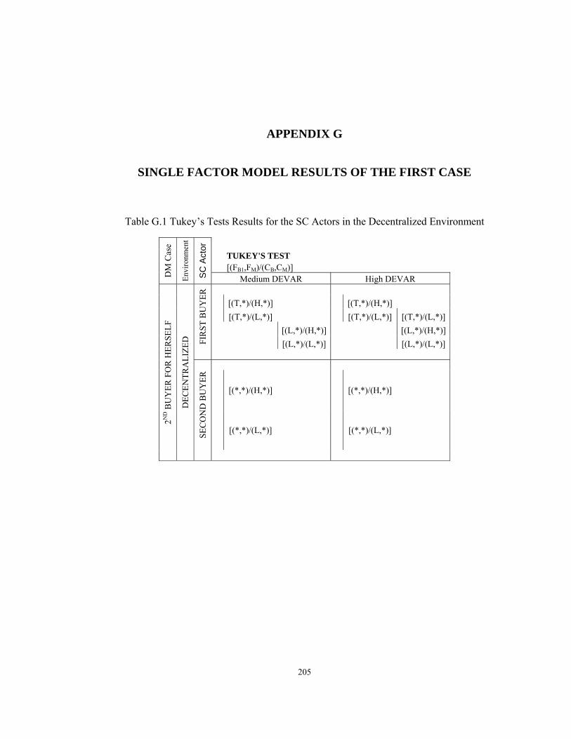
205

APPENDIX G

SINGLE FACTOR MODEL RESULTS OF THE FIRST CASE

Table G.1 Tukey’s Tests Results for the SC Actors in the Decentralized Environment

TUKEY'S TEST [(FB1,FM)/(CB,CM)]

DM

Cas

e

Envi

ronm

ent

SC A

ctor

Medium DEVAR High DEVAR [(T,*)/(H,*)] [(T,*)/(H,*)] [(T,*)/(L,*)] [(T,*)/(L,*)] [(T,*)/(L,*)] [(L,*)/(H,*)] [(L,*)/(H,*)]

FIR

ST B

UY

ER

[(L,*)/(L,*)] [(L,*)/(L,*)]

[(*,*)/(H,*)] [(*,*)/(H,*)]

SEC

ON

D B

UY

ER

[(*,*)/(L,*)] [(*,*)/(L,*)]

2ND B

UY

ER F

OR

HER

SELF

DEC

ENTR

ALI

ZED

206

TUKEY'S TEST [(FB1,FM)/(CB,CM)]

DM

Cas

e

Envi

ronm

ent

SC A

ctor

Medium DEVAR High DEVAR

[(T,T)/(H,H)] [(T,T)/(H,H)]

[(T,T)/(L,H)] [(T,L)/(H,H)]

[(T,L)/(H,H)] [(T,T)/(L,H)]

[(T,L)/(L,H)] [(T,L)/(L,H)]

[(L,T)/(H,H)] [(L,T)/(H,H)]

[(L,T)/(L,H)] [(L,T)/(L,H)]

[(L,L)/(H,H)] [(L,L)/(H,H)]

[(L,L)/(L,H)] [(L,L)/(L,H)]

[(T,T)/(H,L)] [(T,T)/(H,L)]

[(T,T)/(L,L)] [(T,L)/(H,L)]

[(T,L)/(H,L)] [(T,T)/(L,L)]

[(T,L)/(L,L)] [(T,L)/(L,L)]

[(L,T)/(H,L)] [(L,T)/(H,L)]

[(L,T)/(L,L)] [(L,T)/(L,L)]

[(L,L)/(H,L)] [(L,L)/(H,L)]

[(L,L)/(L,L)] [(L,L)/(L,L)]

2ND B

UY

ER F

OR

HER

SELF

DEC

ENTR

ALI

ZED

MA

NU

FAC

TUR

ER

207

Table G.2 Different Results of Duncan’s Tests for the SC Actors in the Decentralized Environment

DUNCAN'S TEST [(FB1,FM)/(CB,CM)]

DM

Cas

e

Envi

ronm

ent

SC A

ctor

Medium DEVAR High DEVAR [(T,*)/(H,*)] [(T,*)/(L,*)] [(T,*)/(L,*)] [(L,*)/(H,*)]

FIR

ST B

UY

ER

[(L,*)/(L,*)]

[(*,*)/(H,*)] [(*,*)/(H,*)]

SEC

ON

D B

UY

ER

[(*,*)/(L,*)] [(*,*)/(L,*)]

[(T,T)/(H,H)]

[(T,T)/(L,H)]

[(T,L)/(H,H)]

[(T,L)/(L,H)]

[(L,T)/(H,H)]

[(L,T)/(L,H)]

[(L,L)/(H,H)]

[(L,L)/(L,H)]

[(T,T)/(H,L)]

[(T,T)/(L,L)]

[(T,L)/(H,L)]

[(T,L)/(L,L)]

[(L,T)/(H,L)]

[(L,T)/(L,L)]

[(L,L)/(H,L)]

[(L,L)/(L,L)]

2ND B

UY

ER F

OR

HER

SELF

DEC

ENTR

ALI

ZED

MA

NU

FAC

TUR

ER

208

Table G.3 Tukey’s Tests Results for the First Buyer in the Centralized Environment

TUKEY'S TEST [(FB1,FM)/(CB,CM)] D

M C

ase

Envi

ronm

ent

SC A

ctor

Medium DEVAR High DEVAR [(L,L)/(L,H)] [(L,T)/(L,H)] [(L,T)/(L,H)] [(L,T)/(L,H)] [(T,T)/(L,H)] [(T,T)/(L,H)] [(T,T)/(L,H)] [(T,T)/(L,H)] [(T,T)/(L,H)] [(T,L)/(L,H)] [(T,L)/(L,H)] [(T,L)/(L,H)] [(T,L)/(L,H)] [(L,L)/(L,H)] [(L,L)/(L,H)] [(L,T)/(H,L)] [(T,L)/(H,H)] [(T,L)/(H,H)] [(L,T)/(H,H)] [(T,T)/(H,H)] [(T,T)/(H,H)] [(L,T)/(L,L)] [(T,T)/(H,L)] [(T,T)/(H,L)] [(L,L)/(H,H)] [(T,L)/(H,L)] [(T,L)/(H,L)] [(T,T)/(H,L)] [(T,T)/(L,L)] [(T,L)/(H,H)] [(T,L)/(L,L)] [(L,L)/(L,L)] [(L,T)/(H,H)] [(L,L)/(H,L)] [(L,L)/(H,H)] [(T,L)/(H,L)] [(L,T)/(H,L)] [(T,T)/(H,H)] [(L,L)/(H,L)] [(T,T)/(L,L)] [(L,T)/(L,L)] [(T,L)/(L,L)] [(L,L)/(L,L)]

2ND B

UY

ER D

ETER

MIN

ES F

OR

HER

SELF

CEN

TRA

LIZE

D

FIR

ST B

UY

ER

209

Table G.4 Tukey’s Tests Results for the Second Buyer in the Centralized Environment

TUKEY'S TEST [(FB1,FM)/(CB,CM)] D

M C

ase

Envi

ronm

ent

SC A

ctor

Medium DEVAR High DEVAR [(L,L)/(L,H)] [(T,T)/(L,H)] [(L,T)/(L,H)] [(L,T)/(L,H)] [(T,L)/(L,H)] [(T,L)/(L,H)] [(T,L)/(L,H)] [(L,T)/(L,H)] [(T,T)/(L,H)] [(T,T)/(L,H)] [(L,L)/(L,H)] [(T,T)/(H,H)] [(T,T)/(H,H)] [(L,T)/(H,L)] [(L,L)/(H,H)] [(L,L)/(H,H)] [(L,T)/(H,H)] [(T,L)/(H,H)] [(T,L)/(H,H)] [(L,L)/(H,H)] [(T,L)/(L,L)] [(T,L)/(L,L)] [(T,T)/(H,H)] [(L,T)/(H,H)] [(L,T)/(H,H)] [(T,T)/(H,L)] [(L,L)/(L,L)] [(L,L)/(L,L)] [(L,L)/(H,L)] [(T,T)/(H,L)] [(T,T)/(H,L)] [(T,L)/(H,H)] [(L,T)/(H,L)] [(L,T)/(H,L)] [(T,L)/(H,L)] [(L,T)/(L,L)] [(L,T)/(L,L)] [(L,T)/(L,L)] [(L,L)/(H,L)] [(L,L)/(H,L)] [(T,T)/(L,L)] [(T,T)/(L,L)] [(T,T)/(L,L)] [(L,L)/(L,L)] [(T,L)/(H,L)] [(T,L)/(L,L)]

2ND B

UY

ER D

ETER

MIN

ES F

OR

HER

SELF

CEN

TRA

LIZE

D

SEC

ON

D B

UY

ER

210

Table G.5 Tukey’s Tests Results for the Manufacturer in the Centralized Environment

TUKEY'S TEST [(FB1,FM)/(CB,CM)] D

M C

ase

Envi

ronm

ent

SC A

ctor

Medium DEVAR High DEVAR [(T,T)/(H,H)] [(T,L)/(H,H)] [(T,L)/(H,H)] [(T,T)/(H,H)] [(L,T)/(H,H)] [(L,L)/(H,H)] [(L,L)/(H,H)] [(L,T)/(H,H)] [(T,L)/(L,H)] [(L,L)/(H,L)] [(T,T)/(L,H)] [(T,L)/(H,L)] [(L,L)/(L,H)] [(T,T)/(H,L)] [(L,T)/(L,H)] [(L,T)/(H,L)] [(T,L)/(H,L)] [(T,L)/(L,H)] [(L,L)/(H,L)] [(T,T)/(L,H)] [(T,T)/(H,L)] [(T,L)/(L,L)] [(L,T)/(H,L)] [(L,L)/(L,L)] [(T,L)/(L,L)] [(T,T)/(L,L)] [(L,L)/(L,L)] [(L,L)/(L,H)] [(T,T)/(L,L)] [(L,T)/(L,H)] [(L,T)/(L,L)] [(L,T)/(L,L)]

2ND B

UY

ER D

ETER

MIN

ES F

OR

HER

SELF

CEN

TRA

LIZE

D

MA

NU

FAC

TUR

ER

211

Table G.6 Different Results of Duncan’s Tests for the First Buyer in the Centralized Environment

DUNCAN'S TEST [(FB1,FM)/(CB,CM)] D

M C

ase

Envi

ronm

ent

SC A

ctor

Medium DEVAR High DEVAR [(L,L)/(L,H)] [(L,T)/(L,H)] [(L,T)/(L,H)] [(L,T)/(L,H)] [(T,T)/(L,H)] [(T,T)/(L,H)] [(T,T)/(L,H)] [(T,L)/(L,H)] [(T,L)/(L,H)] [(T,L)/(L,H)] [(L,L)/(L,H)] [(L,T)/(H,L)] [(L,T)/(H,L)] [(T,L)/(H,H)] [(L,T)/(H,H)] [(L,T)/(H,H)] [(T,T)/(H,H)] [(L,T)/(L,L)] [(L,T)/(L,L)] [(T,T)/(H,L)] [(T,T)/(H,L)] [(L,L)/(H,H)] [(L,L)/(H,H)] [(T,L)/(H,L)] [(T,L)/(H,L)] [(T,L)/(H,L)] [(T,T)/(H,L)] [(T,T)/(H,L)] [(T,T)/(L,L)] [(T,T)/(L,L)] [(T,T)/(L,L)] [(T,L)/(H,H)] [(T,L)/(H,H)] [(T,L)/(L,L)] [(T,L)/(L,L)] [(T,L)/(L,L)] [(L,L)/(L,L)] [(L,T)/(H,H)] [(L,T)/(H,H)] [(L,L)/(H,L)] [(L,L)/(H,H)] [(L,L)/(H,H)] [(T,L)/(H,L)] [(L,T)/(H,L)] [(L,T)/(H,L)] [(T,T)/(H,H)] [(L,L)/(H,L)] [(L,L)/(H,L)] [(T,T)/(L,L)] [(L,T)/(L,L)] [(L,T)/(L,L)] [(T,L)/(L,L)] [(L,L)/(L,L)]

2ND B

UY

ER D

ETER

MIN

ES F

OR

HER

SELF

CEN

TRA

LIZE

D

FIR

ST B

UY

ER

212

Table G.7 Different Results of Duncan’s Tests for the Second Buyer in the Centralized Environment

DUNCAN'S TEST [(FB1,FM)/(CB,CM)] D

M C

ase

Envi

ronm

ent

SC A

ctor

Medium DEVAR High DEVAR [(L,L)/(L,H)] [(T,T)/(L,H)] [(L,T)/(L,H)] [(T,L)/(L,H)] [(T,L)/(L,H)] [(L,T)/(L,H)] [(T,T)/(L,H)] [(L,L)/(L,H)] [(T,T)/(H,H)] [(L,T)/(H,L)] [(L,L)/(H,H)] [(L,T)/(H,H)] [(T,L)/(H,H)] [(L,L)/(H,H)] [(T,L)/(L,L)] [(T,T)/(H,H)] [(L,T)/(H,H)] [(T,T)/(H,L)] [(L,L)/(L,L)] [(L,L)/(H,L)] [(T,T)/(H,L)] [(T,L)/(H,H)] [(L,T)/(H,L)] [(T,L)/(H,L)] [(L,T)/(L,L)] [(L,T)/(L,L)] [(L,L)/(H,L)] [(T,T)/(L,L)] [(T,T)/(L,L)] [(L,L)/(L,L)] [(T,L)/(H,L)] [(T,L)/(L,L)]

2ND B

UY

ER D

ETER

MIN

ES F

OR

HER

SELF

CEN

TRA

LIZE

D

SEC

ON

D B

UY

ER

213

Table G.8 Different Results of Duncan’s Tests for the Manufacturer in the Centralized Environment

DUNCAN'S TEST [(FB1,FM)/(CB,CM)] D

M C

ase

Envi

ronm

ent

SC A

ctor

Medium DEVAR [(T,T)/(H,H)] [(T,L)/(H,H)] [(L,T)/(H,H)] [(L,L)/(H,H)] [(T,L)/(L,H)] [(T,T)/(L,H)] [(L,L)/(L,H)] [(L,T)/(L,H)] [(L,T)/(L,H)] [(T,L)/(H,L)] [(T,L)/(H,L)] [(T,L)/(H,L)] [(L,L)/(H,L)] [(L,L)/(H,L)] [(L,L)/(H,L)] [(T,T)/(H,L)] [(T,T)/(H,L)] [(T,T)/(H,L)] [(L,T)/(H,L)] [(L,T)/(H,L)] [(L,T)/(H,L)] [(T,L)/(L,L)] [(T,L)/(L,L)] [(L,L)/(L,L)] [(L,L)/(L,L)] [(T,T)/(L,L)] [(L,T)/(L,L)]

2ND B

UY

ER D

ETER

MIN

ES F

OR

HER

SELF

CEN

TRA

LIZE

D

MA

NU

FAC

TUR

ER

214

APPENDIX H

SUBCONTRACTING OPTION USED VERSUS REALIZED REPLENISHMENT AMOUNTS THROUGH

FOUR PERIODS

215

Table H.1 Subcontracting Option used versus Total Realized Replenishment Amounts through four Periods in the Decentralized Environment

DECENTRALIZED ENVIRONMENT H / (T,T) / (L,L) First Buyer's Realized Replenishment amounts Second Buyer's Realized Replenishment amounts

1st Period 2nd Period 3rd Period 4th Period 1st Period 2nd Period 3rd Period 4th Period 1st sample 500.0 612.5 714.5 622.7 550.0 720.0 650.0 520.0 2nd sample 500.0 612.5 646.5 552.2 550.0 720.0 740.0 719.9 3rd sample 500.0 612.5 697.9 597.1 550.0 600.0 660.0 650.0 4th sample 500.0 553.9 573.3 529.5 550.0 600.0 700.0 650.0 5th sample 500.0 553.9 573.3 541.0 550.0 600.0 650.0 400.0 6th sample 500.0 600.0 714.5 597.1 550.0 650.0 740.0 719.9 7th sample 500.0 600.0 714.5 605.5 550.0 650.0 780.0 650.0 8th sample 500.0 600.0 650.0 595.4 550.0 720.0 780.0 520.0 9th sample 500.0 553.9 573.3 529.5 550.0 600.0 660.0 650.0

Total Order Amounts Subcontracting option used Total Realized Replenishment given to the Subcontractor versus

Amounts in Four Periods in Four Periods Total Realized Replenishment amounts 4889.8 1340.0 0.27 5041.1 1491.3 0.30 4867.5 1317.7 0.27 4656.7 1106.9 0.24 4368.1 818.3 0.19 5071.6 1521.8 0.30 5050.0 1500.2 0.30 4915.4 1365.7 0.28 4616.7 1066.9 0.23

average: 0.26

216

Table H.2 Subcontracting Option used versus Total Realized Replenishment Amounts through four Periods in the Centralized Environment

CENTRALIZED ENVIRONMENT H / (T,T) / (L,L) First Buyer's Realized Replenishment amounts Second Buyer's Realized Replenishment amounts 1st Period 2nd Period 3rd Period 4th Period 1st Period 2nd Period 3rd Period 4th Period 1st sample 500 660 720 470 550 720 520 650 2nd sample 500 660 480 600 550 720 740 720 3rd sample 500 660 650 470 550 480 780 650 4th sample 500 440 480 470 550 520 780 650 5th sample 500 440 650 440 550 480 520 650 6th sample 500 600 720 440 550 650 740 720 7th sample 500 600 720 600 550 650 780 650 8th sample 500 600 650 470 550 720 780 520 9th sample 500 470 520 470 550 520 740 650

Total Order Amounts Subcontracting option used Total Realized Replenishment given to the Subcontractor versus

Amounts in Four Periods in Four Periods Total Realized Replenishment amounts 4790.0 1060.0 0.22 4970.0 1170.0 0.24 4740.0 1079.6 0.23 4390.0 788.7 0.18 4230.0 630.8 0.15 4920.0 1206.1 0.25 5050.0 1350.0 0.27 4790.0 1032.7 0.22 4420.0 824.9 0.19

average: 0.21

217

APPENDIX I

SINGLE FACTOR MODEL RESULTS OF THE SECOND CASE

Table I.1 Tukey’s Test Results for the SC Actors in the Decentralized Environment

TUKEY'S TEST [(FB2,FM)/(CB,CM)]

DM

Cas

e

Envi

ronm

ent

SC A

ctor

Medium DEVAR High DEVAR

[(*,*)/(H,*)]

[(*,*)/(H,*)]

FIR

ST B

UY

ER

[(*,*)/(L,*)]

[(*,*)/(L,*)]

[(T,*)/(H,*)] [(T,*)/(H,*)]

[(T,*)/(L,*)] [(T,*)/(L,*)] [(T,*)/(L,*)]

[(L,*)/(L,*)] [(L,*)/(H,*)]

SEC

ON

D B

UY

ER

[(L,*)/(H,*)] [(L,*)/(L,*)] MA

NU

FAC

TUR

ER D

ETER

MIN

ES F

OR

2N

D

BU

YER

DEC

ENTR

ALI

ZED

218

[(T,T)/(H,H)] [(T,T)/(H,H)]

[(T,L)/(H,H)] [(T,L)/(H,H)]

[(T,T)/(L,H)] [(L,T)/(H,H)]

[(T,L)/(L,H)] [(L,L)/(H,H)]

[(L,T)/(H,H)] [(T,T)/(L,H)]

[(L,L)/(H,H)] [(T,L)/(L,H)]

[(L,T)/(L,H)] [(L,T)/(L,H)]

[(L,L)/(L,H)] [(L,L)/(L,H)]

[(T,T)/(H,L)] [(T,T)/(H,L)]

[(T,L)/(H,L)] [(T,L)/(H,L)]

[(T,T)/(L,L)] [(L,T)/(H,L)]

[(T,L)/(L,L)] [(L,L)/(H,L)]

[(L,T)/(H,L)] [(T,T)/(L,L)]

[(L,L)/(H,L)] [(T,L)/(L,L)]

[(L,T)/(L,L)] [(L,T)/(L,L)]

MA

NU

FAC

TUR

ER D

ETER

MIN

ES F

OR

2N

D B

UY

ER

DEC

ENTR

ALI

ZED

MA

NU

FAC

TUR

ER

[(L,L)/(L,L)] [(L,L)/(L,L)]

Table I.2 Different Results of Duncan’s Tests for the Second Buyer in the

Decentralized Environment

DUNCAN'S TEST

[(FB2,FM)/(CB,CM)] DM

Cas

e

Envi

ronm

ent

SC A

ctor

High DEVAR

[(T,*)/(H,*)]

[(T,*)/(L,*)] [(T,*)/(L,*)]

[(L,*)/(H,*)]

[(L,*)/(L,*)]MA

NU

FAC

TUR

ER

DET

ERM

INES

FO

R 2

ND

BU

YER

DEC

ENTR

ALI

ZED

SEC

ON

D B

UY

ER

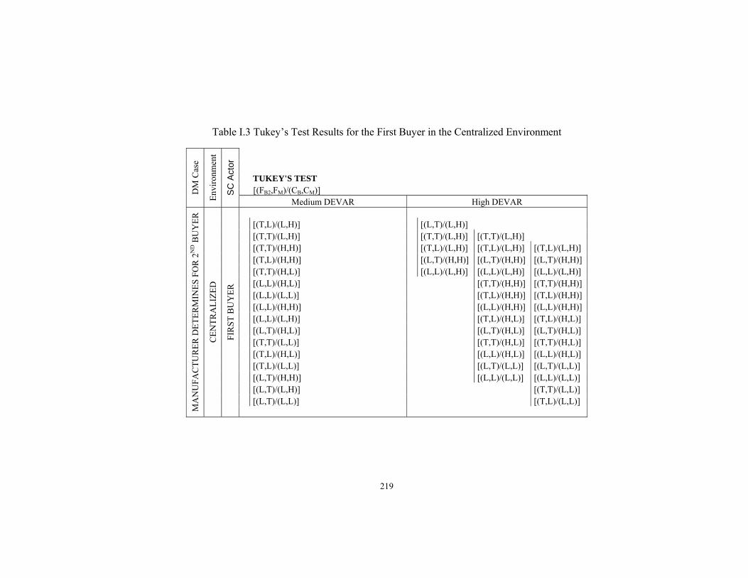
219

Table I.3 Tukey’s Test Results for the First Buyer in the Centralized Environment

TUKEY'S TEST [(FB2,FM)/(CB,CM)] D

M C

ase

Envi

ronm

ent

SC A

ctor

Medium DEVAR High DEVAR [(T,L)/(L,H)] [(L,T)/(L,H)] [(T,T)/(L,H)] [(T,T)/(L,H)] [(T,T)/(L,H)] [(T,T)/(H,H)] [(T,L)/(L,H)] [(T,L)/(L,H)] [(T,L)/(L,H)] [(T,L)/(H,H)] [(L,T)/(H,H)] [(L,T)/(H,H)] [(L,T)/(H,H)] [(T,T)/(H,L)] [(L,L)/(L,H)] [(L,L)/(L,H)] [(L,L)/(L,H)] [(L,L)/(H,L)] [(T,T)/(H,H)] [(T,T)/(H,H)] [(L,L)/(L,L)] [(T,L)/(H,H)] [(T,L)/(H,H)] [(L,L)/(H,H)] [(L,L)/(H,H)] [(L,L)/(H,H)] [(L,L)/(L,H)] [(T,L)/(H,L)] [(T,L)/(H,L)] [(L,T)/(H,L)] [(L,T)/(H,L)] [(L,T)/(H,L)] [(T,T)/(L,L)] [(T,T)/(H,L)] [(T,T)/(H,L)] [(T,L)/(H,L)] [(L,L)/(H,L)] [(L,L)/(H,L)] [(T,L)/(L,L)] [(L,T)/(L,L)] [(L,T)/(L,L)] [(L,T)/(H,H)] [(L,L)/(L,L)] [(L,L)/(L,L)] [(L,T)/(L,H)] [(T,T)/(L,L)] [(L,T)/(L,L)] [(T,L)/(L,L)]

MA

NU

FAC

TUR

ER D

ETER

MIN

ES F

OR

2N

D B

UY

ER

CEN

TRA

LIZE

D

FIR

ST B

UY

ER

220

Table I.4 Tukey’s Test Results for the Second Buyer in the Centralized Environment

TUKEY'S TEST [(FB2,FM)/(CB,CM)] D

M C

ase

Envi

ronm

ent

SC A

ctor

Medium DEVAR High DEVAR [(T,T)/(L,H)] [(L,L)/(L,H)] [(T,L)/(L,H)] [(T,L)/(L,H)] [(L,T)/(L,H)] [(T,T)/(L,H)] [(L,L)/(L,H)] [(L,L)/(L,H)] [(L,T)/(L,H)] [(T,L)/(H,H)] [(T,L)/(H,H)] [(T,L)/(H,H)] [(T,L)/(H,L)] [(T,T)/(H,H)] [(T,T)/(H,H)] [(T,T)/(H,H)] [(T,T)/(H,L)] [(T,T)/(H,L)] [(T,T)/(H,L)] [(T,T)/(H,L)] [(T,L)/(H,H)] [(T,L)/(H,L)] [(T,L)/(H,L)] [(T,L)/(H,L)] [(T,T)/(H,H)] [(T,T)/(L,L)] [(T,T)/(L,L)] [(T,T)/(L,L)] [(T,L)/(L,L)] [(T,L)/(L,L)] [(T,L)/(L,L)] [(T,L)/(L,L)] [(T,T)/(L,L)] [(L,T)/(H,L)] [(L,T)/(H,L)] [(L,T)/(L,L)] [(L,L)/(H,L)] [(L,L)/(H,L)] [(L,L)/(L,L)] [(L,T)/(L,L)] [(L,L)/(H,H)] [(L,L)/(L,L)] [(L,L)/(H,L)] [(L,T)/(H,H)] [(L,T)/(H,L)] [(L,L)/(H,H)] [(L,T)/(H,H)]

MA

NU

FAC

TUR

ER D

ETER

MIN

ES F

OR

2N

D B

UY

ER

CEN

TRA

LIZE

D

SEC

ON

D B

UY

ER

221

Table I.5 Tukey’s Test Results for the Manufacturer in the Centralized Environment

TUKEY'S TEST [(FB2,FM)/(CB,CM)] D

M C

ase

Envi

ronm

ent

SC A

ctor

Medium DEVAR High DEVAR [(T,L)/(H,H)] [(L,T)/(H,H)] [(T,T)/(H,H)] [(L,L)/(H,H)] [(L,T)/(H,H)] [(T,L)/(H,H)] [(L,L)/(H,H)] [(T,T)/(H,H)] [(L,T)/(L,H)] [(L,L)/(H,L)] [(L,L)/(L,H)] [(L,T)/(H,L)] [(T,L)/(H,L)] [(T,L)/(H,L)] [(T,T)/(H,L)] [(T,T)/(H,L)] [(T,L)/(L,H)] [(L,T)/(L,H)] [(T,T)/(L,H)] [(L,L)/(L,H)] [(L,T)/(H,L)] [(T,L)/(L,L)] [(T,L)/(L,L)] [(L,L)/(L,L)] [(L,L)/(H,L)] [(T,T)/(L,L)] [(T,T)/(L,L)] [(T,L)/(L,H)] [(L,T)/(L,L)] [(L,T)/(L,L)] [(L,L)/(L,L)] [(T,T)/(L,H)]

MA

NU

FAC

TUR

ER D

ETER

MIN

ES F

OR

2N

D B

UY

ER

CEN

TRA

LIZE

D

MA

NU

FAC

TUR

ER

222

Table I.6 Different Results of Duncan’s Tests for the First Buyer in the Centralized Environment

DUNCAN'S TEST [(FB2,FM)/(CB,CM)] D

M C

ase

Envi

ronm

ent

SC A

ctor

Medium DEVAR High DEVAR [(T,L)/(L,H)] [(L,T)/(L,H)] [(T,T)/(L,H)] [(T,T)/(L,H)] [(T,T)/(L,H)] [(T,T)/(H,H)] [(T,T)/(H,H)] [(T,L)/(L,H)] [(T,L)/(L,H)] [(T,L)/(H,H)] [(T,L)/(H,H)] [(L,T)/(H,H)] [(L,T)/(H,H)] [(T,T)/(H,L)] [(T,T)/(H,L)] [(L,L)/(L,H)] [(L,L)/(L,H)] [(L,L)/(H,L)] [(L,L)/(H,L)] [(T,T)/(H,H)] [(T,T)/(H,H)] [(L,L)/(L,L)] [(L,L)/(L,L)] [(T,L)/(H,H)] [(T,L)/(H,H)] [(L,L)/(H,H)] [(L,L)/(H,H)] [(L,L)/(H,H)] [(L,L)/(H,H)] [(L,L)/(L,H)] [(L,L)/(L,H)] [(T,L)/(H,L)] [(T,L)/(H,L)] [(L,T)/(H,L)] [(L,T)/(H,L)] [(L,T)/(H,L)] [(L,T)/(H,L)] [(T,T)/(L,L)] [(T,T)/(L,L)] [(T,T)/(H,L)] [(T,T)/(H,L)] [(T,L)/(H,L)] [(T,L)/(H,L)] [(L,L)/(H,L)] [(L,L)/(H,L)] [(T,L)/(L,L)] [(T,L)/(L,L)] [(L,T)/(L,L)] [(L,T)/(L,L)] [(L,T)/(H,H)] [(L,T)/(H,H)] [(L,L)/(L,L)] [(L,L)/(L,L)] [(L,T)/(L,H)] [(L,T)/(L,H)] [(T,T)/(L,L)] [(T,T)/(L,L)] [(L,T)/(L,L)] [(T,L)/(L,L)]

MA

NU

FAC

TUR

ER D

ETER

MIN

ES F

OR

2N

D B

UY

ER

CEN

TRA

LIZE

D

FIR

ST B

UY

ER

223

Table I.7 Different Results of Duncan’s Tests for the Second Buyer in the Centralized Environment

DUNCAN'S TEST [(FB2,FM)/(CB,CM)] D

M C

ase

Envi

ronm

ent

SC A

ctor

Medium DEVAR High DEVAR

[(T,T)/(L,H)] [(L,L)/(L,H)] [(T,L)/(L,H)] [(T,L)/(L,H)] [(L,T)/(L,H)] [(T,T)/(L,H)] [(L,L)/(L,H)] [(L,L)/(L,H)] [(L,T)/(L,H)] [(T,L)/(H,H)] [(T,L)/(H,H)] [(T,L)/(H,L)] [(T,T)/(H,H)] [(T,T)/(H,H)] [(T,T)/(H,L)] [(T,T)/(H,L)] [(T,T)/(H,L)] [(T,T)/(H,L)] [(T,L)/(H,H)] [(T,L)/(H,H)] [(T,L)/(H,L)] [(T,L)/(H,L)] [(T,T)/(H,H)] [(T,T)/(H,H)] [(T,T)/(L,L)] [(T,L)/(L,L)] [(T,L)/(L,L)] [(T,T)/(L,L)] [(L,T)/(H,L)] [(L,T)/(L,L)] [(L,L)/(H,L)] [(L,L)/(L,L)] [(L,T)/(L,L)] [(L,L)/(H,H)] [(L,L)/(L,L)] [(L,L)/(H,L)] [(L,T)/(H,H)] [(L,T)/(H,L)] [(L,L)/(H,H)] [(L,T)/(H,H)]

MA

NU

FAC

TUR

ER D

ETER

MIN

ES F

OR

2N

D B

UY

ER

CEN

TRA

LIZE

D

SEC

ON

D B

UY

ER