Capital Inflows: Macroeconomic Implications and Policy Responses

Roberto Cardarelli, Selim Elekdag, and M. Ayhan Kose

WP/09/40

© 2009 International Monetary Fund WP/09/40 IMF Working Paper Asia and Pacific Department and Research Department

Capital Inflows: Macroeconomic Implications and Policy Responses

Prepared by Roberto Cardarelli, Selim Elekdag, and M. Ayhan Kose1

Authorized for distribution by Stijn Claessens and Joshua Felman

March 2009

Abstract

This Working Paper should not be reported as representing the views of the IMF. The views expressed in this Working Paper are those of the author(s) and do not necessarily represent those of the IMF or IMF policy. Working Papers describe research in progress by the author(s) and are published to elicit comments and to further debate.

This paper examines the macroeconomic implications of, and policy responses to surges in private capital inflows across a large group of emerging and advanced economies. In particular, we identify 109 episodes of large net private capital inflows to 52 countries over 1987–2007. Episodes of large capital inflows are often associated with real exchange rate appreciations and deteriorating current account balances. More importantly, such episodes tend to be accompanied by an acceleration of GDP growth, but afterwards growth has often dropped significantly. A comprehensive assessment of various policy responses to the large inflow episodes leads to three major conclusions. First, keeping public expenditure growth steady during episodes can help limit real currency appreciation and foster better growth outcomes in their aftermath. Second, resisting nominal exchange rate appreciation through sterilized intervention is likely to be ineffective when the influx of capital is persistent. Third, tightening capital controls has not in general been associated with better outcomes.

JEL Classification Numbers: F30; F32; F34

Keywords: Capital inflows, sudden stops, crises, sterilization, capital controls.

Author’s E-Mail Address: rcardarelli@imf.org; selekdag@imf.org; akose@imf.org

1 Earlier versions of this paper were presented at an IMF workshop and the 2009 AEA meetings in San Francisco. We are grateful for helpful comments from Tim Callen, Menzie Chinn, Charles Collyns, Tim Lane, Carlos Vegh and seminar participants. Gavin Asdorian, Stephanie Denis, and Ben Sutton provided excellent research assistance.

2

Contents

I. Introduction ............................................................................................................................4

II. Database and Methodology...................................................................................................6 A. Database ....................................................................................................................6 B. Methodology .............................................................................................................7

III. Capital Inflows: Basic Stylized Facts ................................................................................10 A. Capital Inflows Over Time .....................................................................................10 B. Episodes of Large Capital Inflows ..........................................................................11

IV. Policy Responses to Large Capital Inflows .......................................................................11 A. Exchange Rate Policy .............................................................................................13 B. Sterilization Policy ..................................................................................................17 C. Fiscal Policy ............................................................................................................19 D. Capital Controls ......................................................................................................20

V. Policy Responses: Basic Stylized Facts ..............................................................................22 A. Policy Reponses During Episodes of Large Capital Inflows..................................23

VI. Linking Macroeconomic Outcomes and Policy Responses...............................................24 A. Macroeconomic Outcomes: Basic Stylized Facts...................................................24 B. How to Avoid a Hard Landing After the Inflows?..................................................25 C. How to Contain Real Exchange Rate Appreciation? ..............................................26 D. Any Role for Capital Controls? ..............................................................................27 E. Do Persistence of Inflows and External Imbalances Matter?..................................29

VII. Conclusions ......................................................................................................................30 References................................................................................................................................54 Figures 1. Net Private Capital Inflows to Emerging Markets...............................................................36 2. Mexico: Identification of Large Net Private Capital Inflow Episodes ................................37 3. Gross Capital Flows, Current Account Balance, and Reserve Accumulation.....................38 4. Current Account Balances, Capital Inflows, and Reserves by Region................................39 5. Net FDP and Non-FDI Inflows by Region ..........................................................................40 6. Basic Characteristics of Episodes of Large Net Private Capital Inflows.............................41 7. Exchange Market Pressures (EMP) Across Regions ...........................................................42 8. Exchange Market Pressures, Sterilization, and Government Expenditures.........................43 9. Evolution of Capital Controls ..............................................................................................44 10. Policy Indicators and Episodes of Large Capital Inflows..................................................45 11. Selected Macroeconomic Variables During Large Capital Inflows ..................................46 12. Post-Inflow GDP Growth and Policies ..............................................................................47 13. Real Exchange Rate Appreciation and Policies When Inflation Accelerates....................48

3

14. Macroeconomic Outcomes and Capital Controls ..............................................................49 15. Exchange Market Pressures and Duration of Capital Inflow Episodes .............................50 16. Fiscal Policy and Balance of Payment Pressures...............................................................51 17. Regional Dimensions .........................................................................................................52 Tables 1. List of Net Private Capital Inflow Episodes ........................................................................32 2. Episodes of Large Net Private Capital Inflows: Summary Statistics ..................................33 3. Post-Inflows GDP Growth Regressions...............................................................................34 4. Real Exchange Rate Regressions.........................................................................................35 Appendix..................................................................................................................................53

4

I. INTRODUCTION

The past two decades have witnessed two waves of large capital inflows sweeping through many emerging market economies. The first wave commenced in the early 1990s and ended with the Asian crisis in 1997. The second one started in 2003, and ebbed in 2008 in the wake of the global financial crisis (see Figure 1). While capital inflows often help deliver the economic benefits of increased financial integration, they also create important challenges for policy-makers because of their potential to generate over-heating, loss of competitiveness, and increased vulnerability to crisis.2 In order to mitigate these adverse effects, policies in emerging market countries have responded to large capital inflows in a variety of ways. For example, while some countries have let exchange rates move upwards, in many cases the monetary authorities have intervened heavily in foreign exchange markets to resist currency appreciation. To varying degrees, they have sought to neutralize the monetary impact of intervention through sterilization, with a view to forestalling an excessively rapid expansion of domestic demand. Controls on capital inflows have been introduced or tightened, and controls on outflows eased, to relieve upward pressure on exchange rates. Fiscal policies have also responded—in some cases stronger revenue growth from buoyant activity has been harnessed to achieve better fiscal outcomes, although in many countries rising revenues have led to higher government spending. Interestingly, policy concerns associated with the second wave of large inflows mirrored those in the first half of the 1990s when renewed access to international capital markets in the wake of the resolution of the debt crisis resulted in a surge in the availability of external capital. An important lesson from the earlier period is that the policy choices made in response to the arrival of capital inflows may have an important bearing on macroeconomic outcomes, including the consequences of their abrupt reversal (Montiel, 1999). This paper reviews the experience with large capital inflows over the past two decades in a large number of emerging market and advanced economies, characterizes the various policy responses adopted, and assesses their macroeconomic implications. In particular, we focus on three major questions. First, what are the macroeconomic implications of these episodes? Second, what policy challenges are created by surges of net private capital inflows? Third, and most importantly, what policy measures have been adopted in the past, and did they work? For example, did they help mitigate the risk of sharp reversals of large capital inflows? 2 There has been an intensive debate about the long-term growth benefits of capital inflows in the literature. While some view increasing capital account liberalization and unfettered capital flows as a serious impediment to global financial stability (e.g., Rodrik and Subramanian, 2009), leading to calls for capital controls, some others argue that increased openness to capital flows has, by and large, proven essential for countries aiming to upgrade from lower to middle income status (e.g., Mishkin, 2009). Kose and others (2009), and Obstfeld (2009) present surveys of the large literature about the growth and stability benefits of capital inflows.

5

While a number of earlier studies have examined the policy responses to capital inflows focusing on the experience during the 1990s for a limited number of country case studies, there has been less study of recent episodes and few attempts at a comprehensive cross-country examination of the policy responses. Examples of the first type of studies include Calvo, Leiderman, and Reinhart (1996), Fernández-Arias and Montiel (1996) and Glick (1998).3 In a recent paper, Reinhart and Reinhart (2008) analyze the macroeconomic implications of a large set of surges in capital flows that took place over the period 1980–2007. They document that global factors, including changes in commodity prices, international interest rates, and growth in advanced countries, are the driving forces of international capital flows—echoing the conclusions of earlier work by Calvo and others (1993). They also report that episodes of large inflows tend to end in a variety of economic crises, such as debt defaults, banking crisis, and currency crashes. Our paper contributes to this large literature in at least three major dimensions. First, we identify episodes of large net private capital inflows to a comprehensive sample of advanced and developing countries using a consistent set of criteria. Our methodology leads to 109 episodes of large net private capital inflows to 52 countries over the period 1987–2007, of which 87 episodes were completed by 2006. Second, we provide an extensive discussion of various policy measures and identify these using a wide set of indicators. In particular, we use a variety of quantitative indicators to describe policies regarding the exchange rate, sterilization, the fiscal stance, and capital controls. Moreover, unlike earlier studies, we study the effectiveness of these policy responses to surges in capital inflows considering whether they help a country achieve a soft landing, that is, a moderate decline in GDP growth after the inflows abated. Our findings indicate that episodes of large capital inflows were associated with an acceleration of GDP growth, but afterwards growth often dropped significantly. In fact, post-inflow decline in GDP growth is significantly larger for episodes that end abruptly. Over one third of the completed episodes ended with a sudden stop or a currency crisis, suggesting that “abrupt” endings are not a rare phenomenon. In particular, of the 87 completed episodes, 34 ended with a sudden stop and 13 with a currency crisis. Our results also suggest that the fluctuations in GDP growth have been accompanied by large swings in aggregate demand and in the current account balance, with a strong deterioration of the current account during the inflow period and a sharp reversal at the end. The end of the inflow episodes typically entailed a sharp reversal of non-FDI flows while FDI proved much

3 Kahler, 1998, Montiel (1999), Reinhart and Reinhart (2000), Edwards (2000), and Driver, Sinclair and Thoenissen (2005) are some other studies in the first group. World Bank (1997) provides an early example of a cross-country analysis of policy responses to capital inflows.

6

more resilient. In addition, the surge in capital inflows also appears to be associated with a real effective exchange rate appreciation. With respect to policy choices, four interesting results emerge. First, countries that experience more volatile macroeconomic fluctuations—including a sharp reversal of the inflows—tend to be those with higher current account deficits and with stronger increases in both aggregate demand and the real value of the currency during the period of capital inflows. Second, episodes where the decline in GDP growth following the surge in inflows was more moderate tend to be those in which the authorities exercised greater fiscal restraint during the inflow period, which helped contain aggregate demand and limit real appreciation. This findings suggests that keeping public expenditure growth steady during episodes—rather than ratcheting up spending—can help currency appreciation and foster better macroeconomic outcomes in their aftermath. Third, we find that countries resisting nominal exchange rate appreciation through intervention were generally not able to moderate real appreciation in the face of a persistent surge in capital inflows, and faced more serious adverse macroeconomic consequences when the surge eventually stopped. Fourth, and finally, tightening capital controls has not in general been associated with lower real appreciation, nor with a reduced vulnerability to a sharp reversal of the inflows. The rest of the paper is structured as follows. Section II provides information about our database and methodology used to identify large capital inflows. Next, we document the main stylized facts associated with surges in capital inflows. This is followed by a discussion of possible policy responses to cope with large capital inflows. In section V, we briefly discuss the main features of the policy responses to capital inflows. Section VI establishes empirical links between macroeconomic outcomes and policy responses. Section VII concludes.

II. DATABASE AND METHODOLOGY

A. Database We study the macroeconomic implications of policy responses to surges in capital inflows using a large sample of advanced, emerging, and developing countries. In particular, our dataset comprises annual data over the 1985–2007 period for 52 countries—8 advanced and 44 developing. The latter group includes many emerging market economies while the group of industrial countries corresponds to a sub-sample of the OECD economies which are small and open. We provide the list of these countries in Appendix. Most of our macroeconomic and financial series are from the IMF’s International Financial Statistics. We supplement that

7

with data from various other sources, including the IMF’s World Economic Outlook and Balance of Payments databases. We focus on private capital flows which are based on the nature of the recipient sector. That is, only changes in foreign assets and liabilities of the domestic private sector—as recorded in the IMF’s Balance of Payment (BOP) database—are taken into account, independently of the nature of the foreign counterpart. The main difference compared to a “source” concept of private inflows is the exclusion of sovereign borrowing (specifically, the changes in the government’s assets and liabilities vis-à-vis the foreign private sector) and the inclusion of private borrowing from external official sources. While this difference may be relevant for the early to mid-1990s, it is less likely to be relevant over the recent past, given the decline in sovereign borrowing and official lending. The net private capital inflows series used in the paper are constructed in five steps: First calculate (net) foreign direct investment (FDI) taking direct investments into the recipient country and subtracting direct investments abroad. Second, we strip out assets that are classified under the monetary authority and the general government for each of the remaining categories: portfolio investments, financial derivatives, and other investments. We then do the same for liabilities, in effect yielding assets and liabilities that are private in nature. Third, these series of private assets and liabilities are netted, yielding net inflows for the three categories.4 Fourth, we add FDI to the net private portfolio investment, financial derivative, and other investment categories, yielding our definition of net private capital inflows. Fifth, and finally, we scale the total net private capital inflows by GDP to get the net private capital inflows-to-GDP ratio.

B. Methodology In order to systematically assess countries’ experiences with large net capital inflows, we employ a consistent set of criteria to identify episodes of large net private capital inflows to the countries in our sample that have occurred over the past two decades. Specifically, we employ two criteria which take into account both country- and region-specific dimensions associated with episodes.5 The country-specific dimension of the episodes is captured by the criterion that the ratio of net capital inflows to GDP for a particular country must be significantly larger than the trend of capital inflows to that country. In other words, inflows should be large relative to a country’s historical experience. 4 Note that we add rather than subtract the liabilities because outflows are recorded as negative numbers in the IMF’s BOP presentation.

5 The regions we consider are Latin America, Emerging Asia, Emerging Europe and Commonwealth of Independent States (CIS), and an aggregate group of other emerging market countries. In addition to these, the group of advanced countries is considered as a separate region. See Appendix for the list of countries we use and their distribution into regional groups.

8

The regional dimension is captured by the criterion that capital inflows are significantly larger than a regional threshold, even if they are not out of line with country-specific historical trends. This criterion takes into account that a steady stream of large inflows may have affected the trend of inflows. Therefore, even if inflows are not out of line relative to trend, they still may be large relative to the regional experience. Therefore, an episode is defined as a year or string of years in which at least one of these criteria is met. How does our methodology of identifying episodes work in practice? The episodes are based on the deviations of the net private capital inflows-to-GDP ratio (NPCIR) from its trend. In particular, a rolling, backward looking Hodrick-Prescott (HP) filter is applied to the NPCIR series of each country. A rolling trend was used to capture the real time nature of policy decisions that have been made historically.6 Similar methodologies have been used in the literature, as in, for example, Gourinchas and others (2001). Initially, the first five years of the data is used to determine the trend, with subsequent years added on a rolling basis. The NPCIR series starts well before the 1990s for most cases, which is the sample period we focus on, thereby allowing enough years to establish a stable trend. After we establish the trend, for country i that belongs to region j, we identify a certain year t as an episode year, if either the deviation of NPCIR from its trend in year t is larger than one historical standard deviation, and the NPCIR exceeds 1 percent of GDP, or the NPCIR exceeds the 75th percentile of the distribution of NPCIRs for the region j over the whole sample. Therefore, each episode begins in the first year in which one of these criteria is satisfied, and continues in the subsequent years if they keep meeting these criteria. In effect, a string of episode years makes up an episode. At times, this methodology identifies episodes in clusters. However, such sequences of episodes would make the identification of pre- and post-episode periods ambiguous. As a result, episodes that are too close together would prevent the characterization of how policies and macroeconomic outcomes have evolved before, during, and after the inflow events. Therefore, the criteria discussed above are amended in two ways to ensure that they do not identify any episodes in the two years prior to each episode of large capital inflows: First, if the end-year of an episode immediately precedes the first year of another episode, then the two episodes are combined to form a single episode. Second, if there is only one year between two identified episodes, both episodes are combined to include the year in the middle only if the NPCIR in that middle year is positive. However, if the NPCIR in the year

6 We use a smoothing parameter of 1000 to determine the trend. This trend is quite robust to other values of the smoothing parameter. We choose the smoothing parameter to ensure cross-country consistency so that the episodes identified matched those in the literature. For some countries there is not enough observations to use the rolling HP trend (mostly countries in Central and Eastern Europe). In these cases, the HP filter is applied to the entire NPCIR series, rather than on a rolling basis, using a smoothing parameter of 100.

9

between the two identified episodes is negative, the first episode (usually the one with the lower average NPCIR) is excluded. An important feature of these episodes is how they ended. In particular, an episode is considered to end “abruptly” if the ratio of net private capital inflows to GDP in the year after the episode terminates is more than 5 percentage point of GDP lower than at the end of the episode—closely following the definition of “sudden stops” in the literature (see Mauro and Becker, 2005). An episode is also considered to finish abruptly if its end coincides with a currency crisis, that is, with a steep depreciation of the exchange rate.7 We briefly focus on the case of Mexico to illustrate the mechanics of our methodology. The available NPCIR time series along with the fitted rolling trend and the regional NPCIR threshold (of 4.8 percent of GDP) are shown in Figure 2. The rolling trend depicted in the figure shows the end point of each rolling HP trend. As subsequent years are added to the sample, the HP trend therefore changes, as does its endpoint, by definition. The rolling trend shown in the figure is therefore the series of endpoints based on these sequential trends. To this trend, we add the standard deviations of the NPCIR, which is also updated on a rolling basis consistent with the trend. The year 1990 is identified as an episode year because the inflows to Mexico exceeded the trend by more than one standard deviation. In contrast, the year 1994 is also identified as an event year because, although less than one standard deviation about the rolling trend, inflows in that year were 4.9 percent of GDP, thereby (marginally) exceeding the regional threshold (of 4.8 percent of GDP). Together, the episode years ranging from 1990-1994 comprise a single multi-year episode, whereas 1997 and 2000 are single year episodes.8 It is also worth noting that even though the NPCIR in 1995 declines by only 3 percent relative to 1994, the collapse of the peso in the aftermath of the episode easily meets the Frankel and Rose (1996) definition of currency crises mentioned above, and is therefore counted as an abrupt ending of an episode. We identify 109 episodes of large net private capital inflows since 1987; 87 of these were completed by 2006. We provide the list of these episodes in Table 1. In order to check whether the episodes we identified closely match the historical experiences of the countries in our sample, we compare the inflow episodes examined in the literature with those we identify. Many of the studies in the literature have examined the experience with capital

7 A currency crisis is defined as in Frankel and Rose (1996)—a depreciation of at least 25 percent cumulative over a 12-month period, and at least 10 percentage points greater than in the preceding 12 months.

8 Although episode years were identified in the early 1980s, they were not included in the analysis because our study focuses on the post-1990s experience.

10

flows during the 1990s for a limited number of country case studies.9 The events we identify closely match the episodes discussed in the literature. As some of the identified episodes in 1990s preceded crises, they should be well-known for those familiar with the literature.

III. CAPITAL INFLOWS: BASIC STYLIZED FACTS

In this section, we first briefly document the main stylized facts associated with the temporal dynamics of capital inflows. We then discuss the main features of the episodes of large capital inflows we identified in the previous section.

A. Capital Inflows Over Time

Using the net private capital inflows-to-GDP ratio, Figure 1 shows that there have been two great waves of private capital flows to emerging market countries in the past two decades. The first began in the early 1990s, then ended abruptly with the 1997–98 Asian crisis. The second wave was building since 2002, then accelerated in 2007, with inflows far exceeding 2006. The second wave has started abated in 2008 as the flows of international capital have been curtailed because of the global financial crisis. Looking at the nature and composition of the inflows reveals some interesting differences between the second wave of capital inflows and the one in the 1990s. In particular, the latest wave was taking place in the context of much stronger current account positions for most (but not all) emerging market countries, and a substantial acceleration in the accumulation of foreign reserves (Figure 3). The second surge in private capital inflows was also accompanied by a sharp increase in outflows, in line with the global trend toward the increasing diversification of international portfolios.

Another important feature of the second wave of net capital inflows to emerging markets—which differentiates it from the 1990s—is the predominance of net foreign direct investment (FDI) flows relative to net “financial” flows (portfolio and other flows) in all four regions (Figures 4 and 5). This reflects the continued strength in FDI inflows, together with the rapid increase in financial outflows from emerging markets which has largely offset the acceleration of financial inflows in most of these countries. In sum, the second cycle of capital inflows was different from the previous one, as it involved a larger set of countries, was underpinned by generally more solid current account positions (with the notable exception of emerging European countries), and took taking place

9 The studies we surveyed include Reinhart and Smith (1997), Reinhart and Reinhart (1998), Montiel (1999), Montiel and Reinhart (1999), Ariyoshi and others (2000), Cowan and De Gregorio (2005), Goldfajn and Minella (2005), and Magud and Reinhart (2006). A matrix summarizing the narratives of policy responses to well-documented large capital inflows episodes is available upon request.

11

in a more financially integrated world economy, where significant financial outflows were at least partially offsetting the inflows of capital to emerging markets.

B. Episodes of Large Capital Inflows

As we discuss in the previous section, we identify 109 episodes of large net private capital inflows since 1987 across 52 countries. Viewed from a regional perspective, these episodes show several interesting patterns, broadly in line with the stylized facts documented above: First, the incidence of episodes over time mirrors trends in net private capital inflows to emerging markets, with two waves of episodes of large capital inflows to emerging markets since the late 1980s—one in the mid-1990s and the recent one, starting in 2002 (Figure 6, upper panel). Second, episodes completed during the first wave (between 1987 and 1998) generally involved a smaller volume of flows relative to GDP, especially compared to episodes that were ongoing as of 2007; but they lasted longer than those that ended between 1999 and 2006 (Table 2). Third, Emerging Asian and Latin American countries dominated the first wave of episodes, while the more recent episodes have been more concentrated in emerging Europe and other emerging market countries (Figure 6, middle panel). Fourth, over one third of the completed episodes ended with a sudden stop or a currency crisis (Table 2), suggesting that “abrupt” endings are not a rare phenomenon. In particular, of the 87 completed episodes, 34 ended with a sudden stop and 13 with a currency crisis. In 7 episodes, a sudden stop coincided with a currency crisis. Lastly, our findings also indicate that late and ongoing episodes are characterized by larger FDI flows, relative to the episodes completed in the 1990s (Figure 6, lower panel).

IV. POLICY RESPONSES TO LARGE CAPITAL INFLOWS The influx of large capital inflows has induced policy makers to adopt a variety of measures to prevent overheating and real currency appreciation, and reduce the economy’s vulnerability to a sharp reversal of inflows. These measures include exchange rate intervention, sterilization, fiscal policy, and capital controls. A key policy decision for countries facing large capital inflows is to what extent to resist pressures for the currency to appreciate by intervening in the foreign exchange market (see Lipschitz, Lane, and Mourmouras, 2005; Driver, Sinclair, and Thoenissen, 2005). One of the main motivations for intervention is the concern that massive capital inflows may induce a steep exchange rate appreciation in a short period of time, damaging the competitiveness of export sectors and potentially reducing economic growth. Moreover, if net capital inflows take place in the context of a current account deficit, the real appreciation could exacerbate the external imbalances, heightening the vulnerability to a sharp reversal of capital inflows.

12

However, the accumulation of foreign reserves required to keep the exchange rate from appreciating may lead to excessively loose monetary conditions, thus creating the potential for overheating and financial system vulnerabilities. In this case, the real appreciation could occur via higher inflation, rather than through an increase in nominal exchange rates. Allowing the exchange rate to fluctuate could discourage short-term speculative capital inflows by introducing uncertainty on the changes in the value of the currency (see Calvo and others, 1996). The “impossible trinity” paradigm of open economy macroeconomics—the inability simultaneously to target the exchange rate, run an independent monetary policy, and allow full capital mobility—suggests that, in the absence of direct capital controls, countries facing large capital inflows need to choose between nominal appreciation and inflation (see Obstfeld and Taylor, 2000). In practice, however, given that capital mobility is not perfect—even in the absence of direct capital controls—policy makers may have more scope to pursue intermediate options than this paradigm would suggest, and they have generally used the full menu of available measures.10 When policy makers have intervened to prevent exchange rate appreciation, they have often sought to sterilize the monetary impact of intervention through open market operations and

other measures (such as increasing bank reserve requirements or transferring government deposits from the banking system to the central bank).11 While the motives for sterilization are clear, its effectiveness is less so and it can entail substantial costs. As sterilization is designed to prevent a decline in interest rates, it maintains the incentives for continuing capital inflows, thus perpetuating the problem. Moreover, sterilization often implies quasi-fiscal costs, since it generally involves the central bank exchanging high-yield domestic assets for low-yield reserves. If sterilization is implemented by increasing unremunerated bank reserve requirements, this cost is shifted to the banking system, promoting disintermediation. Fiscal policy is another instrument available to attenuate the effects of capital flows on aggregate demand and the real exchange rate during a surge of inflows and in its aftermath. Fiscal policy in emerging markets receiving capital inflows is typically procyclical, as a fast growing economy generates revenues that feed higher government spending, thus aggravating overheating problems (see Kaminski, Reinhart, and Vegh, 2004). By contrast,

10 See Reinhart and Reinhart (2000), Montiel (1999), and World Bank (1997) for a survey of the theory behind policy responses to capital inflows, and some empirical evidence.

11 With perfect substitution between domestic and foreign assets, maintaining predetermined exchange rates would amount to giving up monetary autonomy, as suggested by the strict form of the “impossible trinity”. Under these circumstances, sterilization would be futile as any uncovered interest rate differential would be quickly eliminated by international interest arbitrage. However, interest rate differentials can and do persist because foreign and domestic assets are not perfect substitutes.

13

greater restraint on expenditure growth has at least three benefits. First, by dampening aggregate demand during the period of high inflows, it allows lower interest rates than otherwise and may therefore reduce incentives for inflows. Second, fiscal restraint alleviates the appreciating pressures on the exchange rate directly, given the bias of public spending toward nontraded goods (see Calvo, Leiderman and Reinhart, 1996). Third, to the extent that it helps address or forestall debt sustainability concerns, it may provide greater scope for a countercyclical fiscal response to cushion economic activity when the inflows stop. While discretionary fiscal tightening during a period of capital inflows may be problematic, due to political constraints and implementation lags, the avoidance of fiscal excesses—holding the line on spending—could play an important stabilization role. In particular, fiscal rules based on cyclically adjusted balances could help resist the political and social pressures for additional spending in the face of large capital inflows. For example, Chile aims at a cyclically-adjusted fiscal surplus, with an additional adjuster to save excess copper revenues, contributing to offset appreciation pressures on the currency In some cases, policymakers in emerging markets have tried to restrict the net inflow of capital by imposing controls on capital inflows or by removing controls on capital outflows. Countries employ such control measures to attain a variety of policy objectives, including discouraging capital inflows to reduce upward pressures on the exchange rate, reducing the risk associated with the sudden reversal of inflows, and maintaining some degree of monetary policy independence. For the purposes of this paper, these policy choices are characterized using across four dimensions. In particular, we use a set of quantitative indicators to describe policies regarding the exchange rate, sterilization, the fiscal stance, and capital controls. We now turn to a discussion of how each of these indicators are developed.

A. Exchange Rate Policy The influx of large net capital inflows tends to put upward pressure on the exchange rate. This often prompts policymakers to adopt a set of policies ranging from outright currency appreciation to intervention in foreign currency markets. To gauge the authorities’ tendency to resist exchange rate appreciations, we first develop a quantitative measure based on an exchange market pressure index. We then use this measure to develop an index of resistance to exchange market pressures, or simply, a resistance index. This index will then determine the degree by which policymakers resist market-based exchange rate fluctuations. Exchange Market Pressures Index

14

Although there are a number of studies presenting methods to measure exchange market pressures (EMP), most of them are derived from the model by Girton and Roper (1977). The idea is that an excess supply of foreign exchange can be met through several, though not mutually exclusive, channels. Therefore, large capital inflows generating an abundance of foreign exchange could be accommodated by a set of policies ranging from a complete offset of pressures by accumulating reserves, or by allowing market forces to bring about an appreciation of the currency. Our EMP measure is a combination of movements in the exchange rate and international reserves (see Bayoumi and Eichengreen, 1998). In theory, for a pure float, the change in the exchange rate would exactly correspond to the index of exchange market pressures. At the other extreme, for a peg, the exchange rate would be constant and fluctuations in EMP would be driven entirely by changes in reserves through intervention. The formal definition of our EMP index comprises several components. First, using monthly data, we define the year-over-year percentage change of the nominal bilateral exchange rate of country i in year t (Δ%eri,t) against a reference country as identified in Levi-Yeyati and Sturzenegger (2005), where an increase implies an appreciation:

, , 1,

, 1

% i t i ti t

i t

er erer

er−

−

−Δ =

Second, using monthly data, we define the year-over-year change in foreign reserves (Δresi,t), where the change in net foreign assets (NFA) is scaled by the lagged value of the monetary base (MB),12 which although standard practice, can be traced back to Girton and Roper (1977):

, , 1,

, 1

i t i ti t

i t

NFA NFAres

MB−

−

−Δ =

Third, we calculate the standard deviations for each year using monthly data for each of these series (Δ%eri,t and Δresi,t). Then, for each year, we compute the regional averages for each of these series, denoting them

,% i terσΔ and ,i tresσΔ , respectively. Hence, these standard deviations

12 Using the IMF’s IFS database, we define NFA=FA – FL, where FA (IFS line 11) and FL (IFS line 16c) denote foreign assets and foreign liabilities, respectively, where the IFS line codes are in parentheses. This data is from the balance sheet of the monetary authority and is converted into U.S. dollars (IFS line ae, end-of-period, bilateral market exchange rate). The monetary base (or reserve money) series (IFS line 14) is also converted in to U.S. dollars.

15

will be different across the five regions we examine, and also over the years in our sample.13 Finally, we define the EMP index that will be used throughout the paper:

, ,

, , ,%

1 1%i t i t

i t i t i ter res

EMP er resσ σΔ Δ

= Δ + Δ

The index is scaled by the individual standard deviations of each component. These weights equalize the volatilities of each component and ensure that neither of them dominates the index as in other studies the literature. Weymark (1997) uses model-consistent weights, and in particular weights that are based on the estimated interest rate elasticity of the demand for money. Pentecost and others (2001) uses principal component analysis to obtain the weights. We follow Eichengreen, Rose and Wyplosz (1996), Kaminsky and Reinhart (1999), and Van Poeck and others (2007), who use variance-smoothing weights. Using regional—rather than country-specific—standard deviations avoids the risk that countries with hardly any significant changes in their exchange rate implicated them with implementing a flexible exchange rate policy owing to the tiny standard deviation of these changes. If exchange rate fluctuations are small, then this would imply a tiny value for the standard deviation of the exchange rate change. In turn, this would inflate the weight on the first term of the EMP (the exchange rate term), thereby causing it to dominate the index spuriously. The use of regional standard deviations alleviates this problem. Bertoli, Gallo, and Ricchiuti (2006) provides a discussion of some of these issues pertaining to EMP indices. There are some other formulations of the EMP index in the literature. For example, a common specification includes a short-term interest rate term. However, such EMP indices have typically been used to determine the episodes of speculative attacks on the currency (see, for example, Eichengreen, Rose, and Wyplosz, 1996). Furthermore, as will be discussed below, we do not want to contaminate the EMP index with an interest rate variable, since we use fluctuations of the short-term interest rate as a separate measure to gauge the stance of monetary policy. Resistance Index Using the EMP index described above, we now present the resistance index that will be used to characterize exchange rate policy throughout the paper. We first scale the first component

13 Consider exchange rates: First, we take the monthly changes, yielding 12 data points for each country in a given year. Second, rather than taking the standard deviation of each country, we take the standard deviation of all of the countries within each of our five regions. The reason we do this is because for some countries the standard deviations are extremely small, which inflates the weights of the EMP.

16

of the EMP by its standard deviation ,, %( % )

i ti t erer σΔΔ . Next, we divide this component by

the EMP index itself. Finally, this ratio is subtracted from unity yielding our resistance to exchange market pressures index, or simply, the resistance index:

Resistance Indexi,t , ,

, ,, ,

% %

% %1

i t i t

i t i ti t i t

er res

er resEMP EMP

σ σΔ Δ

⎡ ⎤ ⎡ ⎤⎛ ⎞ ⎛ ⎞Δ Δ⎢ ⎥ ⎢ ⎥= − =⎜ ⎟ ⎜ ⎟⎜ ⎟ ⎜ ⎟⎢ ⎥ ⎢ ⎥⎝ ⎠ ⎝ ⎠⎣ ⎦ ⎣ ⎦

Although this raw index can take on any values, we standardize it so that it is bounded by the unit interval.14 When the index is equal to 0, it means that no resistance is made to exchange market pressures: Either the exchange rate is allowed to float freely, or a “leaning with the wind” policy is followed that exacerbates the exogenous pressures on the exchange rate, rather than relieving them. For these cases, the index would have negative values. When the index is equal to 1, it means that the maximum amount of resistance is attempted: Either the exchange rate is prevented from moving at all, or extreme forms of a “leaning against the wind” policy are followed that make the exchange rate move in the opposite direction to which it would have occurred in the absence of intervention). These are the cases where the index would have values larger than 1. Intermediate values of the index between 0 and 1 indicate the extent to which market pressures are relieved by intervention in the foreign exchange market. In sum, dividing the changes in foreign reserves by EMP index yields a ratio measuring the proportion of exchange market pressures that are resisted through intervention. Values of the resistance index closer to 1 imply a greater degree of resistance to exchange rate fluctuations. The literature on the EMP is closely related to at least two other strands of research. First, similar to EMP indices, there are measures of exchange rate flexibility. For example, based on the work of Glick, Kretzmer, and Wihlborg (1995), Glick and Wihlborg (1997), Bayoumi and Eichengreen (1998), and Baig (2001) develops a measure of exchange rate flexibility which compares the volatility of exchange rate movements to that of the sum of exchange rate and reserve volatilities. In a sense, this indicator characterizes the degree of relative exchange rate variability to that of reserves. Such indicators seem particularly useful when using higher-frequency data and looking at short-run properties. However, these indicators, because they are based on standard deviations (which can not be negative by definition), will not be able to capture upward or downward pressures on the exchange rate and are therefore less suitable for our purposes. 14 Specifically, if the raw index is negative or zero is given the value of 0; if it’s between 0 and 0.25 is given the value of 0.2; if it’s between 0.25 and 0.5 is given the value of 0.4; if it’s between 0.5 and 0.75 is given the value of 0.6; if it’s between 0.75 and 1, is given the value of 0.8; if it’s 1 or above is given the value of 1.

17

The second strand of the literature focuses on the classification of exchange rate regimes based on the IMF’s Annual Report on Exchange Arrangements and Exchange Restrictions (AREAER), which classifies countries according to their announced regimes. However, what countries report and what they do in practice, in terms of their exchange rate policies, differ (Calvo and Reinhart, 2002). In other words, there is a stark difference between the exchange rate policies announced (de jure) and those implemented (de facto), a finding reinforced by Reinhart and Rogoff (2004). To this end, a branch of the literature has attempted to uncover the actual exchange rate regimes countries try to maintain. Levy-Yeyati and Sturzenegger (2005) use the variability in the exchange rate, the depreciation rate, and international reserves to categorize exchange rate regimes. While it is useful to group countries into certain regimes for each year, it is less so in the context of our paper because we consider episodes which may span several years and therefore regimes.

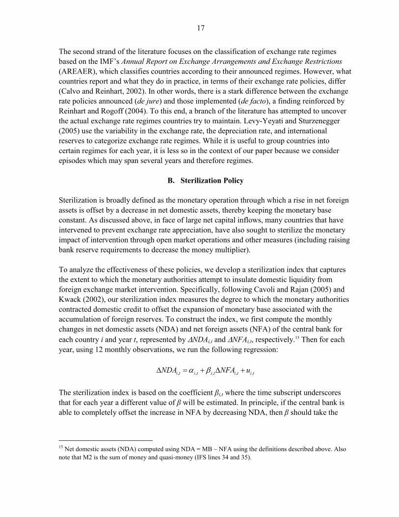
B. Sterilization Policy Sterilization is broadly defined as the monetary operation through which a rise in net foreign assets is offset by a decrease in net domestic assets, thereby keeping the monetary base constant. As discussed above, in face of large net capital inflows, many countries that have intervened to prevent exchange rate appreciation, have also sought to sterilize the monetary impact of intervention through open market operations and other measures (including raising bank reserve requirements to decrease the money multiplier). To analyze the effectiveness of these policies, we develop a sterilization index that captures the extent to which the monetary authorities attempt to insulate domestic liquidity from foreign exchange market intervention. Specifically, following Cavoli and Rajan (2005) and Kwack (2002), our sterilization index measures the degree to which the monetary authorities contracted domestic credit to offset the expansion of monetary base associated with the accumulation of foreign reserves. To construct the index, we first compute the monthly changes in net domestic assets (NDA) and net foreign assets (NFA) of the central bank for each country i and year t, represented by ΔNDAi,t and ΔNFAi,t, respectively.15 Then for each year, using 12 monthly observations, we run the following regression:

, , , , ,i t i t i t i t i tNDA NFA uα βΔ = + Δ + The sterilization index is based on the coefficient βi,t where the time subscript underscores that for each year a different value of β will be estimated. In principle, if the central bank is able to completely offset the increase in NFA by decreasing NDA, then β should take the

15 Net domestic assets (NDA) computed using NDA = MB – NFA using the definitions described above. Also note that M2 is the sum of money and quasi-money (IFS lines 34 and 35).

18

value of –1. In contrast, an estimate of β approaching zero implies little sterilization efforts by the central bank. The second step is to simply multiply β by –1. Therefore, an estimated value of the sterilization index equal to unity implies full sterilization, whereas a value of zero represents no sterilization.16 While we use this index, we also estimate a broader sterilization index that reflects the central bank’s effort to prevent the increase in monetary base from causing an expansion of money supply. This has generally occurred through an increase in the reserve requirements for the banking sector, which reduces the money multiplier. In this case, we follow the steps above except that instead of NDA, the change in M2 is used. The regression equation then takes the form:

, , , , , i t i t i t i t i tNFA vΔΜ2 α δ= + Δ + In this case, the estimated slope coefficient is easy to interpret. Recall that complete sterilization implies that the central bank is able to prevent the increase in NFA from expanding the money supply (M2). Therefore, a value of δ equal to 0 implies full monetary sterilization—NFA fluctuations are not transmitted to M2—whereas a value of 1 represents no sterilization. Although the results based on this broader index are consistent with the ones obtained using the narrower index, we chose to focus on the index based on NDA because it matched some country experiences better. The literature has proposed some other alternatives to measure sterilization policy. These can be broadly categorized into four groups. First, there are those indices based on simple ratios: either the ratio of broad money changes to those in reserves (ΔM2/ ΔNFA), or the ratio of NDA changes to those in reserves (ΔNDA/ ΔNFA) (see Carlson and Hernandez (2002) for the former). Second, there are studies that use the ordinary least squares regression approach we describe above. While these regressions can be augmented by additional explanatory variables, a key assumption made is the exogeneity of capital flows. Third, there are studies that allow for endogeneity, which are based on vector autoregressions (VARs), including work by Christensen (2004) and Moreno (1996). However, as discussed in Takagi and Esaka (1999), there are problems with the VAR approach as well.

16 The sterilization index can also take values larger than unity, which could be interpreted as over sterilization. As mentioned above, sterilization has generally occurred through open market operations, but also in several cases by transferring deposits of the government or pension funds, or the proceeds from privatization of public assets, from the banking system to the central bank. For example, when the authorities offset the purchase of foreign exchange by transferring the government deposits from commercial banks to the central bank, the stock of monetary base is unchanged, as they have exchanged a claim on the domestic banking sector for an external claim.

19

In addition, there are studies that try to assess sterilization policy by estimating a system of simultaneous equations. In contrast with the three methods just described, this approach allows the contemporaneous endogeneity associated with sterilization policy in the context of capital flows: while monetary conditions are affected by capital inflows partly through changes in foreign reserves, international capital flows also respond to changes in domestic monetary conditions, typically through higher interest rates. To this end, studies including Ouyang, Rajan, and Willet (2007) estimate a system of simultaneous equations to measure sterilization policy. While this approach could alleviate endogeneity issues, it requires time series that are available for only a handful of countries used in our sample. Therefore, our sterilization index seems to strike the appropriate balance between technical sophistication and cross-country consistency (also in terms of data requirements). Furthermore, as will be discussed below, our sterilization index generally seems to match country experiences well. A policy of aggressive sterilization usually raises domestic interest rates. The standard mechanism for the increase in interest rates works as follows: to induce investors to hold the increased supply of short-term paper owing to open market operations, the price of this paper need to fall and yields need to increase. In other words, a decrease in central banks’ NDA leads to an increase in interest rates. Therefore, movements in short-term interest rates can be seen as counterparts of changes in central banks’ domestic assets and thus of the sterilization effort. The sterilization index could also be interpreted as a measure for the stance of monetary policy. In practice, however, using the sterilization index as a measure of the monetary policy stance is complicated by the fact that the demand for money balances could be highly unstable, especially in countries with high and volatile inflation (Kaminsky, Reinhart, and Vegh, 2004). Hence, an increase in the monetary base (low sterilization) may not reflect expansionary monetary policy, but simply the accommodation of a higher demand for money. In light of these considerations, we also consider changes in short-term interest rates as an alternative gauge of the monetary policy stance. Since we characterize policies over an entire episode, we are unable to capture the initial bout of aggressive sterilization that is usually the first line of defense against surges of capital inflows. Within an episode, the quasi-fiscal costs of sterilization start adding up over time (usually spanning several months), and its effectiveness diminishes. Therefore, while a country may have implemented a determined policy of sterilization at the onset of large capital inflows, our measure will only capture the average behavior over the entire duration of the episode.

C. Fiscal Policy Another instrument available to mitigate the effects of capital flow surges on aggregate demand and the real exchange rate is countercyclical fiscal policy. We represent the cyclical

20

stance of fiscal policy in response to large net capital inflows by the change in the growth of real noninterest government expenditure. This measure of fiscal policy is useful for at least three reasons. First, because the concept of policy cyclicality is important to the extent that it can help guide actual policy, it makes sense to define policy cyclicality in terms of actual instruments rather than outcomes (which are endogenous, including, for example, fiscal balances). Second, although both government spending and tax rates can gauge the cyclical stance of fiscal policy, there is no systematic data on tax rates. Third, As emphasized by Kaminsky, Reinhart, and Vegh (2004), considering fiscal variables as a proportion of GDP, could yield misleading results because the cyclical stance of fiscal policy may be dominated by the cyclical behavior of output. Following Gavin and Perotti (1997), Braun (2001), Dixon (2003), Lane (2003), and Calderon and Schmidt-Hebbel (2003), we use the real noninterest government expenditure growth to measure to stance of fiscal policy.17 To complement this indicator, we also calculate the deviation of real government spending from trend, using the Hodrick-Prescott filter. This is an attempt to refine our primary measure towards achieving a structurally adjusted characterization of the fiscal policy stance.

D. Capital Controls Capital controls are one of the more controversial choices available to policymakers during periods of large net capital flows. They are used to meet certain policy objectives, including discouraging capital inflows outright, thereby reducing upward pressures on the exchange rate, lowering the risk associated with asset prices bubbles and the sudden reversal of inflows, and maintaining some degree of monetary policy independence. We mainly focus on the implications of the temporary use of capital controls during the periods of inflow surges in countries with fairly liberalized capital accounts. Nonetheless, there is a large literature analyzing the growth and stability outcomes of capital controls for countries at different stages of the liberalization process (see Kose and others, 2009). We first present a conceptual framework motivating both the theoretical and practical rationales for implementing capital controls. From a theoretical viewpoint, the perspective of a simple neoclassical model is useful. In such a model capital inflows—assumed to be foreign direct investment (FDI) in its purest form—increase a country’s stock of physical capital thereby supporting growth. Along with the assumption of an abundant supply of foreign capital implies that a country should borrow capital to the point where the marginal value of capital is equal to the world interest rate. However, if the supply of capital is upward

17 The IMF’s World Economic Outlook (WEO) database was used to produce this measure. First, interest expenditures were subtracted from government expenditures (using WEO codes: GGENL – GGEI). Then, nominal noninterest expenditures were scaled by CPI (WEO code PCPI) to yield the real noninterest government expenditure series.

21

sloping, the increasing marginal cost of capital implies as argued by Cardoso and Goldfajn (1998) a restriction of capital inflows below the competitive level, offering a rationale for using taxes or quantitative restrictions on foreign borrowing. However, departing from the simple model discussed above, theory indicates that controls can be welfare reducing, unless they are a “second-best” option that mitigates the effects of another market failure (see Neely, 1999). In a survey on market distortions and second-best arguments that justify intervention over international capital transactions, one type of market failure cited by Dooley (1995) is myopic private speculation. Rodrik and Velasco (1999) and Rodrik and Subramanian (2009) present both theoretical and empirical arguments making a case for discouraging (short-term) inflows. Stiglitz (2004) provides two theoretical models whereby increased financial market integration leads to increased income and consumption volatility. Although capital controls cover a wide range of measures regulating inflows and outflows of foreign capital, they generally take two broad forms: direct (or administrative) and indirect (or market-based) controls. Direct controls are associated with administrative measures, such as direct prohibitions and explicit limits on the volume of transactions. For example, Malaysia introduced a set of direct capital controls in 1998 involving various quantitative restrictions on cross-border trade of its currency and credit transactions (to dampen large net capital outflows). As another example of the direct taxation of inflows, Brazil created a facility for fixed income investments subject to an ‘entrance tax’ on the initial exchange rate transaction in 1994. Indirect capital controls include explicit or implicit taxation of financial flows and differential exchange rates for capital transactions. For example, in order to discourage capital inflows, Chile imposed an implicit tax in 1991 in the form of an unremunerated reserve requirement (URR) on specified inflows for up to one year (the encaje); which was substantially relaxed in 1998. In 1993, Colombia also implemented a variation of a URR. The traditional approach to measuring capital controls is based on the IMF’s Annual Report on Exchange Arrangements and Exchange Restrictions (AREAER) which provides information on different types of controls. Early work quantifying the narrative descriptions in the AREAER has simply used a binary measure (Grilli and Milesi-Ferretti, 1995). More sophisticated approaches use finer measures of controls, but still essentially summarize the information in the AREAER (Chinn and Ito, 2006; Edwards, 2005; Miniane, 2004; Mody and Murshid, 2005; and Quinn, 2003). With the expansion of the set of control categories and further refinements in the 1996 issue of the AREAER, it is now possible to distinguish between controls on inflows from those on outflows beginning in 1995 (see Schindler, 2009). Therefore, in line with previous studies, the degree to which the authorities restrict net inflows of capital by imposing administrative controls on capital inflows is captured through

22

an index based on the IMF’s AREAER. The same source is used to construct a second index that measures the degree to which authorities react to the surge in capital inflows by liberalizing a variety of restrictions on capital outflows.18 That said, it is a challenge to effectively quantify the extent of capital controls. In particular, it would be desirable to capture the degree of enforcement of capital controls. Moreover, the impact of a measure would depend on a broad assessment of the openness of the capital account. Our measure of capital controls, like others in the literature, are inherently coarse. This implies that even if a country may have tightened controls on inflows, our measure may not be able to detect such policy changes at times.

V. POLICY RESPONSES: BASIC STYLIZED FACTS Recent years have seen substantial changes in the use of these various policy responses compared to the 1990s. The second wave of capital inflows has been associated with strong exchange market pressures in all regions, which have been resisted through the accumulation of foreign reserves, while also allowing some upward movements in exchange rates (Figure 7). This pattern is significantly different from the earlier wave of net capital inflows, when, for most emerging market countries, pressures on exchange rates were negative, reflecting large current account deficits, and exchange rates typically depreciated. Emerging Asia was the one region experiencing positive exchange market pressures over 1994–96, but these pressures were absorbed through reserve accumulation. The fact that foreign exchange reserves increased over the 1990s may indicate an asymmetry in the response to exchange rate pressures, with a tendency to intervene to prevent the appreciation of the currency, but not to stem a depreciation (except when the pressures became extreme in a financial crisis, as shown by the large reduction of reserves in 1997 in emerging Asia and in 2001 in Latin America and other emerging markets). Over the period 2004–2007, there has been substantial exchange rate appreciation in the face of high and rising positive exchange market pressures, reflecting the trend toward increasing exchange rate flexibility in many countries, especially in emerging Asia. Nevertheless, the relatively

18 The AREAER has indices on nine different dimensions of capital controls, both on inflows and outflows, including controls on capital and money market instruments, on direct investment, and on personal capital movements. The types of controls covered in the 1996 AREAER and beyond include controls on capital and money market instruments, credit operations, derivatives and other instruments, direct investment, personal capital movements, real estate transactions, provisions specific to commercial banks and other credit institutions, and institutional investors, and lastly, surrender requirements. Along with many other studies, the indices used in this paper are the averages across these nine dimensions. Note that the AREAER published before 1996, although similar in scope, is not as detailed as the newer refined versions. Also, whereas the latest AREAER distinguishes between controls on inflows and outflows separately, the older vintages do not. Nonetheless, in line with Miniane (2004), we utilize the more detailed coverage in the recent AREAER, but then backcast both indices in proportion to the older pre-1996 AREAER vintages.

23

high values of the resistance index in all emerging market regions over the recent past reflects the continued widespread desire to limit the extent of exchange rate appreciation (Figure 8, top panel). The degree of sterilization has seen some convergence across regions (Figure 8, middle panel). The high values of the index in the early 1990s and the early 2000s—the beginning of the two waves of large capital inflows—suggest an aggressive sterilization effort when capital begins to pour in. This index subsequently tapers off around 2006, perhaps indicating that, as intervention continued, the authorities became increasingly conscious of its cost.19 The pattern of real government expenditure reveals that in the emerging market countries considered in our sample, real government expenditure growth accelerated starting in 2005, especially in Latin America and emerging Europe and the CIS (Figure 8, bottom panel). Finally, the indices of capital controls in emerging market regions (Figure 9) suggest that controls on capital inflows have been relaxed since the late 1990s, although in the aggregate the changes have been relatively slow. Emerging European and CIS countries have moved furthest, with emerging Asian countries remaining quite restrictive. Restrictions on residents’ capital outflows have also been progressively loosened in emerging Europe and the CIS, and other emerging market regions, and only more recently in emerging Asia and Latin America, with the latter region starting from a relatively more open position.

A. Policy Reponses During Episodes of Large Capital Inflows

How do the policy responses change during the episodes we identified? To answer this question, for each episode, the averages of policy indicators over the years of the episodes, the two years before its beginning and the two years after its end are first estimated. We report the medians across these averages in the figures because the median is a measure of central tendency that is robust to episodes that may be outliers. We split the set of identified episodes into groups according to various criteria and employ a statistical test that will assess whether the medians across these groups are equivalent or not.20

19 At the same time, the slight decline of the index over the last two decades could reflect both the increased degree of financial integration—that heightens the substitutability of domestic and foreign assets and thus makes sterilization less effective—and the increased demand for money balances from lower inflation and higher output growth—which reduced the need to sterilize the inflationary impact of the increase in reserves.

20 We use a nonparametric test based on the work by Wilcoxon (1945) and Mann and Whitney (1947) which tests the null hypothesis that the two groups were drawn from populations with the same median. The rank-based nonparametric test is based on the comparison of the number of observations above and below the overall median in each subgroup, and is sometimes referred to as the median test (Conover, 1980). Under the null hypothesis, the median chi-squared test statistic is asymptotically distributed as chi-squared with one degree of freedom in the case of two subgroups. If the null is rejected at the 10 percent level of better, then the test indicates that the difference between the medians across the two groups of episodes is genuinely different.

24

Looking specifically at the episodes of large capital inflows, the policy responses are characterized by the following general trends (see Figure 10). First, the resistance index tends to increase during an episode. This is especially the case for episodes completed before 1998 for which the increase in the index during the inflow period is statistically significant, based on the nonparametric test discussed above. Second, sterilization does not tend to increase during an episode, relative to the two years beforehand. This result seems consistent with the temporary nature of the sterilization efforts during the episodes discussed above, as many countries were unable to sustain aggressive sterilization over the inflow periods, at least partly because of the associated quasi-fiscal costs. Third, real government expenditures tend to increase strongly as capital inflows surge, suggesting that fiscal policy has generally been procyclical. Finally, controls on inward capital flows appear to have been tightened (even if not significantly so) during the episodes completed before 1998. By contrast, during the more recent episodes capital controls appear to have been eased, in line with the general trend toward increased financial integration and greater capital mobility. For completed episodes, the surge of capital inflows has not coincided with a relaxation of controls on capital outflows. However, these restrictions appear to be less strict during the ongoing episodes.

VI. LINKING MACROECONOMIC OUTCOMES AND POLICY RESPONSES In this section, we first document some basic stylized facts regarding the dynamics of key macroeconomic indicators in the context of large capital inflows. We then examine the macroeconomic consequences of the policy responses to large capital inflows. Our analysis focuses especially on how successful these policies were in reducing the economy’s vulnerability to an abrupt and costly end to the inflows.

A. Macroeconomic Outcomes: Basic Stylized Facts To document the basic stylized facts associated with macroeconomic outcomes, we study the behavior of real GDP growth, real aggregate demand, the current account balance, and the real effective exchange rate before, during, and after the episodes (Figure 11). We report four major results. First, episodes of large capital inflows were associated with an acceleration of GDP growth, but afterwards growth has often dropped significantly. In fact, post-inflow decline in GDP growth is significantly larger for episodes that end abruptly. In these cases, average GDP growth in the two years after the end of the episodes tends to be about 3 percentage points lower than during the episode, and about 1 percentage point lower than during the two years before the episode. This suggests that for episodes ending abruptly, it may take some time to fully recover from the economic slowdown associated with such hard landings.

25

Second, the fluctuations in GDP growth have been accompanied by large swings in aggregate demand and in the current account balance, with a strong deterioration of the current account during the inflow period and a sharp reversal at the end. Third, consistent with the literature on capital outflows, the end of the inflow episodes typically entailed a sharp reversal of non-FDI flows, while FDI proved much more resilient. Fourth, the surge in capital inflows also appears to be associated with a real effective exchange rate appreciation, but the lack of statistical significance in the difference between median appreciation before and during the surge in capital inflows reflects the considerable variation across country experience. Moreover, the mechanism generating real appreciation during an episode has not, on average, been higher inflation. This reflects the fact that, for a significant group of episodes, the surge in capital inflows occurred in the context of inflation stabilization plans.21

B. How to Avoid a Hard Landing After the Inflows? In light of the stylized facts documented above, an important test of the effectiveness of policies during the inflow period is whether they helped a country achieve a soft landing, that is, a moderate decline in GDP growth after the inflows abated. Episodes characterized by a sharper post-inflow decline in GDP growth tend to be those with a faster acceleration in domestic demand, a sharper rise in inflation, and a larger real appreciation during the inflow period (Figure 12, upper panel). These episodes are also those that lasted longer, as shown by the much higher cumulative size of the inflows. Examples in this group of episodes are Thailand 1988–96, Argentina 1992–94 and 1997–99, and Mexico 1990–94. Hence, the sharper post-inflow decline in GDP growth seems to be associated with persistent, expansionary capital inflows, which compound external imbalances and sow the seeds of the eventual sharp reversal. From a policy perspective, it is striking that “hard landings” have also been associated with a strong increase in government spending during the inflow period, while expenditure restraint helps reduce upward pressures on both aggregate demand and the real exchange rate and facilitates a soft landing (Figure 12, lower panel).22 By contrast, a higher degree of resistance

21 Examples are Peru 1992–97, Brazil 1994–96, Bulgaria 1992–93, and Latvia 1994–95. As noted in Calvo and Vegh (1999), except for the behavior of inflation, exchange rate based-inflation stabilization typically leads to the same outcome as an “exogenous” capital inflow, that is, a surge in capital inflows, a pick-up in aggregate demand, and a larger real appreciation of the domestic currency that, together with larger current account deficits, sow the seeds of a much stronger decline in GDP growth at the end of the episodes.

22 The fiscal policy indicator reported in this and following figures is the cyclical component of government spending. The same results are obtained using the growth in real government spending.

26

to exchange rate changes during the inflow period and a greater degree of sterilization were unable to prevent real appreciation, and generally unsuccessful in achieving a soft landing. As said before, this may reflect the fact that sterilization efforts tend to induce higher nominal interest rates and thus perpetuate the inflows (Reinhart and Reinhart, 1998). The results of basic cross-section regressions on the sample of events confirm the correlation between post-inflows GDP growth and the macroeconomic policies captured by the event analysis. It is important to underscore that these regressions are to assess whether the associated discussed thus far, hold up when controlling for multiple factors. That is, the regressions should be interpreted as a multivariate correlation analysis, rather than seen as implying any causal relationships. In particular, Table 3 shows that countercyclical fiscal policy through expenditure restraint during the episodes of large capital inflows is associated with a smaller post-inflow decline in GDP growth, even after controlling for other factors that may have had a role in this decline—such as changes in the terms of trade, world output growth, and the real U.S. Fed funds rate. The regressions also present evidence indicating that greater resistance to exchange market pressures is associated with a sharper economic slowdown in the aftermath of the episodes–possibly an implication of the larger relative price adjustment associated with this strategy, as we discuss in the next subsection. Moreover, episodes that ended with a “sudden stop” tend to have a sharper decline of GDP growth in the aftermath of the episode, and also tend to be associated with a higher resistance to exchange market pressures—20 of the 34 episodes that ended with a “sudden stop” are characterized by a high (above median) value of the resistance index.23 However, while these regressions help analyze the correlation between the dependent and policy variables in a multivariate context, we recognize that they do not control for the endogeneity and should therefore not be interpreted as indicating a causal relationship among them.

C. How to Contain Real Exchange Rate Appreciation? The earlier findings suggest that a smaller real appreciation in response to large capital inflows may help reduce an economy’s vulnerability to a sharp and costly reversal. But what policies have been effective in containing upward pressures on the exchange rate? Splitting the episodes between those with high (above-median) real appreciation and those with low (below-median) real appreciation offers a first attempt at answering this question.24

23 In the regression, external factors—real U.S. fund rate and world output growth—also matter, suggesting that countries’ policy responses may not entirely circumvent a reversal of the inflows associated with changes in global factors.

24 The correlation between the extent of real appreciation and macroeconomic policies is analyzed here only in the context of episodes during which inflation accelerated—43 of the total 109 episodes—as these are more likely to be driven by an exogenous shock to capital inflows, rather than exchange-rate based inflation stabilization programs.

27

Figure 13 reveals that greater real appreciation has been associated with a stronger acceleration of CPI inflation, more sterilized intervention, and rising government expenditure. These results suggest that a policy of sterilized intervention is unlikely to prevent real appreciation, and often tends to be associated with higher inflation. As discussed above, the increasing quasi-fiscal costs of sterilization may eventually induce policymakers to give up complete sterilization efforts: the additional liquidity from incomplete sterilization may then add to inflationary pressures. Moreover, in these episodes, a greater increase in nominal interest rates—that is, a more countercyclical monetary policy—is strongly associated with greater real appreciation, as higher returns on domestic assets end up attracting more capital inflows and fueling the upward pressures on the currency. In contrast, countercyclical fiscal policy in the form of slower growth in government expenditure is again strongly associated with lower real appreciation. Finally, tighter controls on capital flows do not appear to be associated with lower real appreciation as we discuss later. To assess the strength of these correlations, a cross-section regression was run on the sample of events. This relates the extent of real exchange rate appreciation during the period of capital inflows to the policy responses we considered along with other factors that may also lead to real appreciation—including the cumulative size of the inflows, movements in the terms of trade, and changes in the output gap. The results support the conclusion that a policy of resistance to exchange market pressures does not seem to be associated with lower real appreciation, while countercyclical fiscal policies have had the desired effect (Table 4). As mentioned above, the main purpose of these regressions was to assess a multivariate association between the real exchange rate and our policy measures, controlling for other factors that may influence the dependent variable.

D. Any Role for Capital Controls? We now investigate the role of capital controls using the episodes of large inflows we identified. Episodes characterized by tighter controls on inflows are associated with narrower current account deficits and lower net private inflows, including lower net FDI flows (Figure 14, top panel). While stricter inflow controls are accompanied by lower-post inflow growth and a larger appreciation of the currency, these distinctions are not statistically significant. In contrast, inflation rates have been significantly higher in episodes with tighter controls. Does having capital controls in place reduce vulnerability to financial crises and sudden stops? Episodes that ended in an abrupt reversal of net inflows do not seem to be associated

28

with lower capital controls (Figure 14, bottom panel).25 Using the full sample of episodes, the results suggest that there has not been any statistically significant change in the median of capital controls during episodes relative to the periods before or after. Consistent with this finding, recent studies also document that countries with capital controls are in fact more susceptible to crises (Glick, Guo, and Hutchison, 2006). This could simply be because of a “selection effect”—often it is countries with weaker macroeconomic fundamentals that put controls in place to insulate themselves from crises. However, these studies find that, even after controlling for such effects, countries with controls have a higher likelihood of currency crises and sudden stops. Moreover, there seems to be little empirical evidence that the output costs of currency and banking crises are smaller in countries that restrict capital mobility. Another policy used by some countries to cope with large net inflows was the removal of controls on outflows. Evidence based on the wave of inflows during the 1990s suggests that elimination of controls on outflows has often led to larger inflows.26 However, our findings suggest that, in about 40 percent of episodes where rising gross outflows offset gross inflows, countries indeed relaxed capital controls on outflows. Most of these episodes occurred during the 2003–2006 period. In an attempt to gauge the robustness of these associations, we included a measure of capital controls to the regressions discussed above. More precisely, we added our measure of capital inflow restrictions based on the IMF’s AREAER as an explanatory variable to both the post-inflow growth and the real exchange rate specifications. We also tried the other measures of capital controls (including the one developed by Edwards, 2005) to assess the sensitivity of these additional regressions. Our findings indicate that while more restrictive controls on inflows may help avoid hard landings, none of the capital control measures is statistically significant in the real exchange rate equations.27

25 The evolution of capital controls is also examined using the full sample of episodes. The results suggest that there has not been any significant change in the median of capital controls during episodes relative to the periods before or after. 26 Liberalizing outflow restrictions may attract heavier inflows by sending a positive signal to markets increasing investor confidence, and thereby fuelling even larger inflows (Bartolini and Drazen, 1997), which is supported by evidence based on several countries (Reinhart and Reinhart, 1997). Edwards (2007) collects a number of recent studies about the effectiveness of capital controls. Analyzing the link between capital controls and interest rate differentials, Straetmans, Versteeg and Wolff (2008) report that capital controls do not provide governments extra monetary policy independence.

27 As an additional check, we also used the capital control measure developed by Edwards (2005), which is only statistically significant for the more parsimonious post-inflow growth regressions (the first three columns of Table 3). Overall, these results resonate the mixed findings in the literature regarding the macroeconomic implications of capital controls.

29

It is hard to draw a set of general results from the earlier literature about the effectiveness of capital controls as most of the studies are based on specific country cases (Ariyoshi and others, 2000). Overall, these studies suggest that controls on inflows did not affect the volume of net flows in most countries, although it seems that they were able to temporarily tilt the composition toward longer maturities in a few cases (Chile after 1991, see Edwards and Rigobon, 2005). Moreover, stricter controls on outflows appeared to reduce net capital flows and allow more independent monetary policy in Malaysia after 1998, but there is little support for such outcomes in other countries (Magud and Reinhart, 2007). Even in cases where a narrow range of objectives were met, controls had only temporary effects as market participants eventually found ways to circumvent them. Although there is little evidence that capital controls are effective at achieving their macroeconomic objectives beyond a limited period, they are associated with substantial microeconomic costs especially when they are sustained for a prolonged period of time (Kose and others, 2009). For example, capital controls are estimated to make it more difficult and expensive for small firms to raise capital (Forbes, 2007a). Moreover, multinational affiliates located in countries with capital controls face local borrowing costs that are much higher than affiliates of the same parent company borrowing locally in countries without capital controls (Desai, Foley, and Hines, 2004). Moreover, economic behavior is likely to be distorted by capital controls, and resources are wasted in seeking to circumvent controls (Johnson and Mitton, 2003; Forbes, 2007b). Capital controls also increase the cost of engaging in international trade even for those firms that do not intend to evade them because of expenses incurred to meet various inspection and reporting requirements associated with controls (Wei and Zhang, 2006). In sum, our results echo the mixed findings in the literature regarding the macroeconomic implications of capital controls. While capital controls may have macroeconomic benefits for certain countries, they also most certainly bring about microeconomic distortions discussed above. Capital controls are no substitute for sound macroeconomic policies including a prudent fiscal stance and a supporting exchange rate and monetary policy framework, as well as appropriate prudential measures.

E. Do Persistence of Inflows and External Imbalances Matter? Before concluding, we discuss three additional issues that warrant consideration: the persistence of inflow episodes, the initial current account positions, and regional factors. The policy responses and outcomes appear to depend on the persistence of inflows. For example, episodes that lasted less than two years display somewhat different patterns than longer episodes, with significantly larger resistance to exchange rate changes, less real appreciation and better post-inflow GDP growth (Figure 15, upper panel). However, these results do not show that resistance is more effective in such cases, as during short inflow episodes higher

30

resistance was not associated with significantly smaller real appreciation or better post-inflow growth (Figure 15, lower panel). This suggests that resisting exchange market pressures may be more feasible when facing transitory inflows, but does not generate significantly better outcomes. Moreover, in practice it may be difficult for policy makers to identify ex ante when an episode of inflows will turn out to be temporary. In addition, the fiscal policy response appears to have been less decisive in episodes associated with high balance of payment pressures (defined as an above-median sum of the current account and net private capital inflows). For such episodes, lower government spending growth is not associated with significantly lower real appreciation or better post-inflow GDP growth (Figure 16, upper panel). By contrast, fiscal spending restraint is associated with significantly better outcomes when the episodes are characterized by low balance of payment pressures (Figure 16, lower panel). This suggests that a countercyclical policy stance may be most important when inflows occur in the context of a large current account deficit. The importance of fiscal restraint in reducing the degree of real exchange rate appreciation and in smoothing GDP fluctuations in the periods surrounding the episodes is also borne out from a regional perspective. The regions with stronger real appreciation during the episodes, Latin America and emerging Europe and the CIS, are also those with larger increases in public expenditure in those periods (Figure 17). By contrast, the advanced economies we considered, which have followed more countercyclical fiscal policies and have refrained from resisting exchange market pressures, appear to have experienced less real appreciation and smaller GDP growth fluctuations around the episodes.

VII. CONCLUSIONS

We analyze the lessons from the experience of large net private capital inflows over the last two decades, especially with regard to the macroeconomic consequences of the policy choices made in response to these inflows. While countries’ response to a surge of capital inflows depends on the specific nature of the inflows as well as on various aspects of their particular circumstances and objectives, four general patterns emerge from a systematic review of inflow episodes: First, countries with relatively high current account deficits have been more vulnerable to a sharp reversal of capital inflows, as they have been particularly affected by the increase in aggregate demand and the real appreciation of their currencies. Second, a clear policy message is that public expenditure restraint—rather than ratcheting up spending—during such episodes can contribute to a lower real exchange rate appreciation and a better post inflow GDP growth performance. Third, a policy of resistance to nominal exchange rate appreciation has not generally been successful in preventing real appreciation, and has often been followed by a sharper reversal of capital inflows, especially when these inflows have

31

persisted for a longer time. Fourth, and finally, our results suggest that restrictions on capital inflows have generally not been associated with lower real appreciation and softer landings at the end of episodes. These findings imply that the stabilization challenges from large capital inflows are most serious for countries with substantial current account imbalances. Especially in the context of relatively inflexible exchange rate policies, the most effective tool available to policymakers to avoid overheating and output instability is likely to be fiscal restraint. Our results also suggest that, even if a central bank initially intervenes to resist nominal exchange rate appreciation when capital inflows begin, this stance should be progressively relaxed if the inflows persist. This is because it becomes less likely that such a policy will succeed in avoiding real appreciation and a painful end to the inflows. The appropriate policy response to large capital inflows of course depends on a variety of country-specific circumstances, including the nature of the underlying inflows—in particular, the extent to which they reflect domestic or external factors and the extent to which the inflows are expected to be persistent—the stage of the business cycle and the fiscal policy situation. In addition, the quality of domestic financial markets also matters. Nevertheless, our findings do provide helpful guidance as to what has worked, and not worked, in the past. In addition to the macroeconomic policy instruments that form the focus of our paper, the policy makers have other tools at their disposal, which have not been analyzed systematically—notably financial supervision and regulation, but also a wider range of policies such as labor and product market reforms. The role of such policies in responding to capital inflows would be an important topic for future research.

32

Table 1. List of Net Private Capital Inflow Episodes

Cumulative Size Cumulative SizeCountry Duration (percent of GDP) Country Duration (percent of GDP)

Albania 1997 4.3 Malaysia 1989 – 1996 79.1Albania 2000 2.6 Malta 1993 – 2000 60.2Argentina 1992 – 1994 11.6 Malta ongoing since 2005 17.1Argentina 1997 – 1999 11.0 Mexico 1990 – 1994 26.3Australia 1988 – 1990 16.8 Mexico 1997 6.2Australia 1995 – 1999 24.8 Mexico 2000 4.9Australia ongoing since 2003 24.5 Morocco 1989 – 1994 21.0Brazil 1994 – 1996 11.3 Morocco 1997 – 2001 22.7Brazil 2000 – 2001 7.0 New Zealand 1992 7.0Bulgaria 1992 – 1993 7.4 New Zealand 1995 – 1997 19.0Bulgaria ongoing since 1997 118.4 New Zealand 2000 5.9Canada 1997 – 1998 3.8 New Zealand ongoing since 2004 31.4Chile 1988 – 1997 70.5 Norway 1993 4.3China 1993 – 1995 12.6 Norway 1996 – 1997 6.5China 2004 5.6 Pakistan 1991 – 1996 18.1Colombia 1993 – 1996 20.2 Pakistan ongoing since 2005 7.1Colombia 2004 – 2005 6.0 Paraguay 1994 – 1997 10.1Costa Rica 1987 – 1992 16.0 Paraguay 2005 4.5Costa Rica 1995 5.3 Peru 1992 – 1997 39.6Costa Rica 1999 6.1 Philippines 1987 – 1997 59.6Costa Rica ongoing since 2002 32.4 Poland 1995 – 2000 35.0Croatia 1997 – 1999 29.9 Romania 1990 – 1993 9.5Croatia ongoing since 2002 59.0 Romania 1996 – 1998 14.2Cyprus 1989 – 1992 21.4 Romania ongoing since 2004 42.3Cyprus 1997 3.3 Russia 2003 1.8Cyprus 1999 – 2001 15.5 Russia ongoing since 2006 4.1Cyprus ongoing since 2005 23.2 Singapore 1990 – 1991 16.2Czech Republic 1994 – 1995 24.0 Slovak Republic 1996 – 1998 31.4Czech Republic 2000 – 2002 26.3 Slovak Republic 2002 21.1Denmark 1994 5.8 Slovak Republic 2005 14.2Denmark 1997 5.0 Slovenia 1997 5.0Denmark 1999 5.1 Slovenia 2001 – 2002 14.7Egypt 1992 2.8 South Africa 1995 3.3Egypt 1997 – 1998 8.2 South Africa 2000 1.8Egypt ongoing since 2005 6.9 South Africa ongoing since 2004 12.4Estonia 1996 – 1998 38.6 Sweden 1988 – 1990 15.2Estonia ongoing since 2002 74.4 Sweden 1998 – 2000 14.4Hong Kong SAR 1997 7.5 Thailand 1988 – 1996 88.8Hong Kong SAR 2000 2.5 Thailand ongoing since 2005 12.2Hungary 1991 – 2000 75.3 Tunisia 1990 – 1994 19.8Hungary 2005 9.4 Tunisia 1998 – 1999 6.3Iceland 1996 – 2000 29.6 Tunisia ongoing since 2004 12.8Iceland ongoing since 2003 77.1 Turkey 1992 – 1993 4.4India 1988 – 1990 6.9 Turkey 1995 – 2000 15.3India 1994 3.2 Turkey ongoing since 2003 25.7India ongoing since 2002 18.3 Ukraine 2005 7.5Indonesia 1990 – 1996 26.3 Uruguay 1997 1.5Israel 1995 – 1997 17.4 Uruguay 2000 1.6Korea 1990 – 1996 18.9 Uruguay ongoing since 2005 12.0Korea 1999 – 2000 4.7 Venezuela 1991 – 1993 10.8Korea 2003 3.4 Venezuela 1997 – 1998 6.3Latvia 1994 – 1995 19.3 Vietnam 1994 9.1Latvia ongoing since 2001 84.7 Vietnam 1999 10.1Lithuania 1997 – 1998 21.0 Vietnam ongoing since 2003 38.4Lithuania ongoing since 2005 20.5

Source: Authors’ calculations. Note: Cumulative size refers to the cumulative net private capital inflows during episodes.

33

Table 2. Episodes of Large Net Private Capital Inflows: Summary Statistics

Completed Completedduring during All

1987-1998 1999-2006 Ongoing Episodes

Number of episodes 53 34 22 109

Average size (percent of GDP) /1 4.7 5.1 7.5 5.1(5.3) (5.8) (8.7) (6.1)

Duration (years) /1 3 1.5 3 2(3.3) (2.6) (3.6) (3.1)

Ended abruptly (number of episodes) 26 14 - 40

in sudden stop 22 12 - 34 in currency crisis 10 3 - 13

Source: Authors’ calculations. 1/ Median across episodes; means in parenthesis.

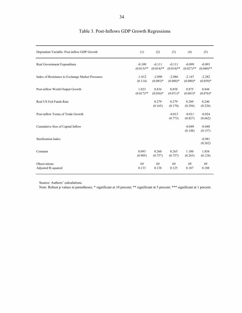
34

Table 3. Post-Inflows GDP Growth Regressions

Dependent Variable: Post-inflow GDP Growth (1) (2) (3) (4) (5)

Real Government Expenditure -0.109 -0.111 -0.111 -0.099 -0.093(0.015)** (0.014)** (0.014)** (0.027)** (0.040)**

Index of Resistance to Exchange Market Pressures -1.812 -2.090 -2.086 -2.147 -2.282(0.114) (0.085)* (0.088)* (0.080)* (0.059)*

Post-inflow World Output Growth 1.023 0.836 0.858 0.875 0.844(0.017)** (0.056)* (0.071)* (0.063)* (0.076)*

Real US Fed Funds Rate 0.279 0.279 0.209 0.240(0.165) (0.170) (0.294) (0.226)

Post-inflow Terms of Trade Growth -0.013 -0.011 -0.024(0.773) (0.827) (0.662)

Cumulative Size of Capital Inflow -0.049 -0.048(0.148) (0.157)

Sterilization Index -0.981(0.262)

Constant 0.093 0.260 0.265 1.100 1.854(0.905) (0.757) (0.757) (0.263) (0.124)

Observations 69 69 69 69 69Adjusted R-squared 0.133 0.138 0.125 0.187 0.188

Source: Authors’ calculations. Note: Robust p values in parentheses; * significant at 10 percent; ** significant at 5 percent; *** significant at 1 percent.

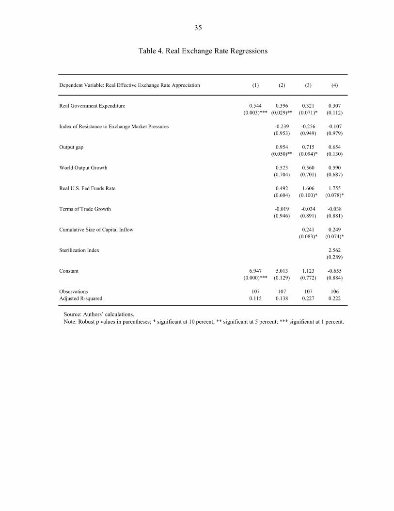
35

Table 4. Real Exchange Rate Regressions

Dependent Variable: Real Effective Exchange Rate Appreciation (1) (2) (3) (4)

Real Government Expenditure 0.544 0.396 0.321 0.307(0.003)*** (0.029)** (0.071)* (0.112)

Index of Resistance to Exchange Market Pressures -0.239 -0.256 -0.107(0.953) (0.949) (0.979)

Output gap 0.954 0.715 0.654(0.050)** (0.094)* (0.130)

World Output Growth 0.523 0.560 0.590(0.704) (0.701) (0.687)

Real U.S. Fed Funds Rate 0.492 1.606 1.755(0.604) (0.100)* (0.078)*

Terms of Trade Growth -0.019 -0.034 -0.038(0.946) (0.891) (0.881)

Cumulative Size of Capital Inflow 0.241 0.249(0.083)* (0.074)*

Sterilization Index 2.562(0.289)

Constant 6.947 5.013 1.123 -0.655(0.000)*** (0.129) (0.772) (0.884)

Observations 107 107 107 106Adjusted R-squared 0.115 0.138 0.227 0.222

Source: Authors’ calculations. Note: Robust p values in parentheses; * significant at 10 percent; ** significant at 5 percent; *** significant at 1 percent.

36

Figure 1. Net Private Capital Inflows to Emerging Markets

-1

0

1

2

3

4

5

6

7

8

9

10

1985 1990 1995 2000 2005-100

0

100

200

300

400

500

600

700

800

900

1000

Net private capital inflows (percent of total emerging market GDP, left scale)

Net private capital inflows (billions of U.S. dollars, right scale)

Sources: IMF, Balance of Payments Statistics; and authors’ calculations. Note: Value for 2008 are IMF staff projections.

37

Figure 2. Mexico: Identification of Large Net Private Capital Inflow Episodes

-15.0

-13.0

-11.0

-9.0

-7.0

-5.0

-3.0

-1.0

1.0

3.0

5.0

7.0

9.0

11.0

1970 1973 1976 1979 1982 1985 1988 1991 1994 1997 2000 2003 2006

Rolling trend

Rolling trend plus one standard deviation

Net Private Capital Flows(percent of GDP)

75th Percentile of Net Private

Capital Flow for Region

Episode year

Sources: IMF Balance of Payments Statistics; and authors’ calculations.

38

Figure 3. Gross Capital Flows, Current Account Balance, and Reserve Accumulation

-4

-2

0

2

4

6

8

10

12

1985 1990 1995 2000 2005-4

-2

0

2

4

6

8

10

12Current account balance

Gross private inflows

Gross private outflows

Accumulation of reserves

Sources: IMF, Balance of Payments Statistics and World Economic Outlook databases; and authors’ calculations. Note: Flows in percent of regional GDP; values for 2008 are IMF World Economic Outlook estimates.

39

Figure 4. Current Account Balances, Capital Inflows, and Reserves by Region

Latin America

-15

-10

-5

0

5

10

15

20

1985 1990 1995 2000 2005-15

-10

-5

0

5

10

15

20

Gross private capital inflowsGross private capital outflows

Accumulation of reservesCurrent accountNet private capital inflows

Emerging Asia

-15

-10

-5

0

5

10

15

20

1985 1990 1995 2000 2005-15

-10

-5

0

5

10

15

20

Gross private capital inflowsGross private capital outflows

Accumulation of reservesCurrent accountNet private capital inflows

Emerging Europe

-15

-10

-5

0

5

10

15

20

1985 1990 1995 2000 2005-15

-10

-5

0

5

10

15

20

Gross private capital inflowsGross private capital outflows

Accumulation of reservesCurrent accountNet private capital inflows

Other Emerging Markets

-15

-10

-5

0

5

10

15

20

1985 1990 1995 2000 2005-15

-10

-5

0

5

10

15

20

Gross private capital inflowsGross private capital outflows

Accumulation of reservesCurrent accountNet private capital inflows

Sources: IMF, Balance of Payments Statistics and World Economic Outlook databases; and authors’ calculations. Note: Flows in percent of regional GDP; values for 2008 are IMF World Economic Outlook estimates.

40

Figure 5. Net FDP and Non-FDI Inflows by Region

Latin America

-6

-4

-2

0

2

4

6

1985 1990 1995 2000 2005-6

-4

-2

0

2

4

6

Net FDI inlfowsNet portfolio inflowsNet other inflows

Emerging Asia

-6

-4

-2

0

2

4

6

1985 1990 1995 2000 2005-6

-4

-2

0

2

4

6

Net FDI inlfowsNet portfolio inflowsNet other inflows

Emerging Europe

-6

-4

-2

0

2

4

6

1985 1990 1995 2000 2005-6

-4

-2

0

2

4

6

Net FDI inlfowsNet portfolio inflowsNet other inflows

Other Emerging Markets

-6

-4

-2

0

2

4

6

1985 1990 1995 2000 2005-6

-4

-2

0

2

4

6

Net FDI inlfowsNet portfolio inflowsNet other inflows

Sources: IMF, Balance of Payments Statistics and World Economic Outlook databases; and authors’ calculations. Note: Flows in percent of regional GDP; values for 2008 are IMF World Economic Outlook estimates.

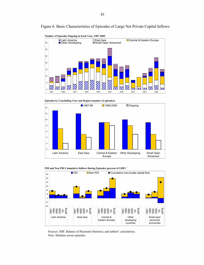
41

Figure 6. Basic Characteristics of Episodes of Large Net Private Capital Inflows

Number of Episodes Ongoing in Each Year, 1987-2005

Episodes by Concluding Year and Region (number of episodes).

FDI and Non FDI Cumulative Inflows During Episodes (percent of GDP) 1

0

5

10

15

20

25

30

35

1987 1989 1991 1993 1995 1997 1999 2001 2003 2005

Latin America East Asia Central & Eastern EuropeOther Developing Small Open Advanced

0

2

4

6

8

10

12

14

Latin America East Asia Central & EasternEurope

Other Developing Small OpenAdvanced

1987-98 1999-2006 Ongoing

-20

-10

0

10

20

30

40

50

60

1987

-19

9819

99-

2006 On

goin

g

1987

-19

9819

99-

2006 On

goin

g

1987

-19

9819

99-

2006 On

goin

g

1987

-19

9819

99-

2006 On

goin

g

1987

-19

9819

99-

2006 On

goin

g

Latin America East Asia Central &Eastern Europe

Otherdevelopingcountries

Small openadvancedeconomies

FDI Non-FDI Cumulative net private capital flow

Sources: IMF, Balance of Payments Statistics; and authors’ calculations. Note: Medians across episodes.

42

Figure 7. Exchange Market Pressures (EMP) Across Regions Latin America Other Emerging Markets

East Asia Small Open Advanced Economies

Central and Eastern Europe

-0.8

-0.6

-0.4

-0.2

0.0

0.2

0.4

0.6

0.8

1.0

1.2

1.4

1991 1992 1993 1994 1995 1996 1997 1998 1999 2000 2001 2002 2003 2004 2005 2006 2007

-1.5

-1.0

-0.5

0.0

0.5

1.0

1.5

1991 1992 1993 1994 1995 1996 1997 1998 1999 2000 2001 2002 2003 2004 2005 2006 2007

-2.0

-1.5

-1.0

-0.5

0.0

0.5

1.0

1.5

1991 1992 1993 1994 1995 1996 1997 1998 1999 2000 2001 2002 2003 2004 2005 2006 2007

-0.8

-0.6

-0.4

-0.2

0.0

0.2

0.4

0.6

0.8

1.0

1.2

1991 1992 1993 1994 1995 1996 1997 1998 1999 2000 2001 2002 2003 2004 2005 2006 2007

-2.5

-2.0

-1.5

-1.0

-0.5

0.0

0.5

1.0

1.5

1991 1992 1993 1994 1995 1996 1997 1998 1999 2000 2001 2002 2003 2004 2005 2006 2007

Change in exchange rates Change in reserves EMP

Source: Authors’ calculations.

43

Figure 8. Exchange Market Pressures, Sterilization, and Government Expenditures

Index of Resistance to Exchange Market Pressures

0.0033620.445199

-0.0177480.097496

-0.0242710.0771040.3727520.1785980.2599220.3226380.366253

0.250570.417094

0.67307

Sterilization Index

Real Government Expenditure Growth Rate

0.0

0.1

0.2

0.3

0.4

0.5

0.6

0.7

0.8

0.9

1.0

1991 1992 1993 1994 1995 1996 1997 1998 1999 2000 2001 2002 2003 2004 2005 2006 2007

Latin America East AsiaCentral and Eastern Europe Other Emerging MarketsAdvanced Economies

-0.6

-0.4

-0.2

0.0

0.2

0.4

0.6

0.8

1.0

1.2

1.4

1991 1992 1993 1994 1995 1996 1997 1998 1999 2000 2001 2002 2003 2004 2005 2006

-16

-12

-8

-4

0

4

8

12

16

20

1990 1991 1992 1993 1994 1995 1996 1997 1998 1999 2000 2001 2002 2003 2004 2005 2006

Source: Authors’ calculations. Note: Unweighted average of country-specific indicators.

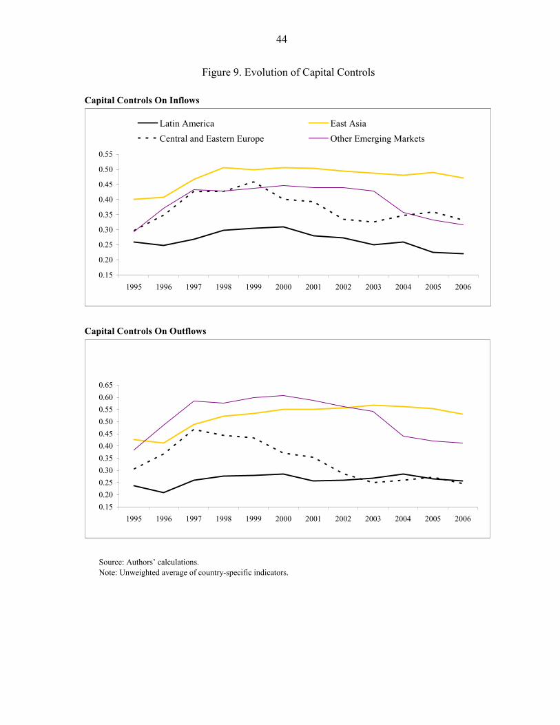
44

Figure 9. Evolution of Capital Controls Capital Controls On Inflows

Capital Controls On Outflows

0.15

0.20

0.25

0.30

0.35

0.40

0.45

0.50

0.55

1995 1996 1997 1998 1999 2000 2001 2002 2003 2004 2005 2006

Latin America East AsiaCentral and Eastern Europe Other Emerging Markets

0.150.200.250.300.350.400.450.500.550.600.65

1995 1996 1997 1998 1999 2000 2001 2002 2003 2004 2005 2006

Source: Authors’ calculations. Note: Unweighted average of country-specific indicators.

45

Figure 10. Policy Indicators and Episodes of Large Capital Inflows Index of Resistance to Exchange Market Pressures Sterilization Index

Real Government Expenditure Growth (in percent) Index of Controls on Capital Inflows

Index of Controls on Capital outflows

0.0

0.1

0.2

0.3

0.4

0.5

0.6

0.7

0.8

0.9

1.0

Episodes completed in1987-98

Episodes completed in1999-2006

Ongoing Episodes

Before During

0.0

1.0

2.0

3.0

4.0

5.0

6.0

7.0

8.0

9.0

10.0

Episodes completed in1987-98 (*)

Episodes completed in1999-2006 (*)

Ongoing Episodes

Before During

0.0

0.1

0.2

0.3

0.4

0.5

0.6

0.7

0.8

Episodes completed in1987-98 (*)

Episodes completed in1999-2006

Ongoing Episodes

Before During

0.00

0.05

0.10

0.15

0.20

0.25

0.30

0.35

0.40

0.45

Episodes completed in1987-98

Episodes completed in1999-2006

Ongoing Episodes

Before During

0.00

0.05

0.10

0.15

0.20

0.25

0.30

0.35

0.40

0.45

0.50

Episodes completed in 1987-98

Episodes completed in 1999-2006

Ongoing Episodes

Before During

Sources: IMF’s AREAER and IFS databases; and authors’ calculations. Note: Medians across episodes. “Before” (“After”) denotes averages of the indicators in the two years before (after) the episodes. The arrows indicate that the difference between medians is significant at a 10 percent level or better. For example, in the top left panel, the average resistance indexes during the episodes completed in 1987–1998 are statistically significantly different than the average resistance indexes in the two years before those episodes.

46

Figure 11. Selected Macroeconomic Variables During Large Capital Inflows

Real GDP Growth (percent) Current Account Balance (percent of GDP)

Real Domestic Demand Growth (percent) Real Exchange Rate Appreciation (percent)

CPI inflation (percent) Nominal Exchange Rate Appreciation (percent)

FDI Net Inflows (percent of GDP) Non-FDI Net Inflows (percent of GDP)

0

1

2

3

4

5

6

Before During After

-3.5

-3.0

-2.5

-2.0

-1.5

-1.0

-0.5

0.0

Before During After

-1.5

-1

-0.5

0

0.5

1

1.5

2

2.5

3

3.5

Before During After

0.0

0.5

1.0

1.5

2.0

2.5

3.0

3.5

4.0

4.5

5.0

Before During After

0

0.5

1

1.5

2

2.5

Before During After-1

-0.5

0

0.5

1

1.5

2

2.5

3

Before During After

0

1

2

3

4

5

6

7

8

9

Before During After-7

-6

-5

-4

-3

-2

-1

0

Before During After

Source: Authors’ calculations. Note: Medians across episodes. “Before” (“After”) denotes averages of the indicators in the two years before (after) the episodes. Arrows indicate that differences between medians are significant at the 10 percent level or better. Effective exchange rates used. Nominal (effective) exchange rate appreciation is the cumulative change within periods.

47

Figure 12. Post-Inflow GDP Growth and Policies Selected Macroeconomic Variables /1

Policy Indicators /1

-5 0 5 10 15 20

Post-Inflow GDP growth * /2

Real domestic demand growth * /3

CPI inflation /4

Current Account Balance /4

Real exchange rate appreciation * /5

Cumulative Size of Inflows * /7

Episodes with the weakest post-inflow GDP growthEpisodes with the strongest post-inflow GDP growth

-1.5 -1.0 -0.5 0.0 0.5 1.0 1.5 2.0 2.5

Real government expenditure * /6

Nominal interest rate /3

Index of resistance to exchange market pressure /4

Sterilization Index /4

Controls on capital inflows /4

Controls on capital outflows /4

Episodes with the weakest post-inflow GDP growthEpisodes with the strongest post-inflow GDP growth

Source: Authors’ calculations. 1/ Values reported are medians for the two groups of episodes. Episodes with the weakest strongest) post-inflow GDP growth are those with above (below) median difference between average GDP growth in the two years after the episode and the average during the episodes. The asterisk (*) indicates that the difference between medians is significant at a 10 percent level or better. 2/ In percent. Average real GDP growth in the two years after the episodes less average during episodes. 3/ In percent. Average during episodes minus average in the two years before the episode. 4/ In percent, but current account balance in percent of GDP. Average during episodes. 5/ In percent. Cumulative change during episodes. 6/ In percent. Average deviations from the (Hodrick-Prescott filter determined) trend of real government noninterest expenditure during the episodes minus the average in the two years before the episode. 7/ In percent of GDP.

48

Figure 13. Real Exchange Rate Appreciation and Policies When Inflation Accelerates 1/

-4.0 -2.0 0.0 2.0 4.0 6.0 8.0

CPI inflation /2

Real exchange rate appreciation * /3

Real government expenditure * /4

Nominal interest rate * /2

Index of Resistance to exchange market pressure /5

Sterilization Index* /5

Index of controls on capital inflows /5

Index of controls on capital outflows /5

Episodes with low REER appreciationEpisodes of high REER appreciation

Source: Authors’ calculations. 1/ Values reported are medians for the two groups of episodes. Episodes with high (low) real effective exchange rate (REER) appreciation are those with above (below) median cumulative REER appreciation in the group of events for which CPI inflation accelerates during the episode. The asterisk (*) indicates that the difference between medians is significant at a 10 percent confidence level or better. 2/ In percent. Average during the episode minus the average in the two years before episodes. 3/ In percent. Cumulative change during the episode. 4/ In percent. Average deviations from (Hodrick-Prescott filter determined) trend of real noninterest government expenditure during the episodes, minus the average in the in the two years before the episodes. 5/ Average during episodes.

49

Figure 14. Macroeconomic Outcomes and Capital Controls Capital Controls and Selected Macroeconomic Series 1/

Endings of Episodes and Controls on Capital Inflows 6/

-6.0 -4.0 -2.0 0.0 2.0 4.0 6.0 8.0 10.0

Post-Inflow GDP growth 2/

CPI inflation * 3/

Current account balance * 4/

Real exchange rate appreciation 5/

Average net private capital flow * 4/

Average net FDI 3/

Episodes with low capital controlsEpisodes with high capital controls

0.00

0.05

0.10

0.15

0.20

0.25

0.30

0.35

0.40

0.45

Before During After

Smooth endings Abrupt endings

Sources: IMF’s Annual Report on Exchange Arrangements and Exchange Restrictions (AREAER), Balance of Payments Statistics, International Financial Statistics databases, and authors’ calculations. 1/ Values reported are medians for the two groups of episodes. Episodes with high (low) capital controls are those with above (below) median values of the capital controls index discussed in the text, where higher (lower) values indicate tighter (looser) regulation of inflows. The asterisk (*) indicates that the differences between medians is significant at a 10 percent level or better. 2/ In percent. Average real GDP growth in the two years after the episodes less average during episodes. 3/ In percent. Average during episodes. 4/ In percent of GDP. Average during episodes. 5/ In percent. Cumulative change during episodes. 6/ Median value across all completed episodes using the index of capital controls discussed in the text where higher values indicate tighter regulation of inflows. “Before” denotes averages of the index in the two years before the episodes. “After” denotes averages of the index in the two years after the episodes.

50

Figure 15. Exchange Market Pressures and Duration of Capital Inflow Episodes 1/ Duration of Episodes

Index of Resistance to Exchange Market Pressures in One- or Two-Year Episodes

-6.0 -5.0 -4.0 -3.0 -2.0 -1.0 0.0 1.0 2.0 3.0

Post Inflow GDP growth * 2/

Current Account Balance * 3/

Real exchange rate appreciation 4/

Nominal exchange rate appreciation* 4/

Real government expenditures 5/

Index of resistance to exchange market pressures * 3/

Sterilization Index 3/

Index of controls on capital inflows * 3/

Index of controls on capital outflows * 3/

Episodes with duration 1-2 yearsEpisodes with duration 3+ years

-1.0 -0.5 0.0 0.5 1.0 1.5

Index of resistance to exchangemarket pressures * 3/

Post Inflow GDP growth 2/

Real exchange rate appreciation 4/

Nominal exchange rate appreciation4/

Episodes with low resistanceEpisodes with high resistance

Source: Authors’ calculations. 1/ Values reported are medians for the two groups of episodes. The asterisk (*) indicates that the difference between medians is significant at a 10 percent confidence level or better. 2/ In percent. Average in the two years after the episode minus the average during the episode. 3/ Average during the episode. Current account balance in percent of GDP. 4/ In percent. Average deviations from (Hodrick-Prescott filter determined) trend of real noninterest government expenditure during the episodes, minus the average in the in the two years before the episodes.

51

Figure 16. Fiscal Policy and Balance of Payment Pressures 1/

Duration of Episodes

Index of Resistance to Exchange Market Pressures in One- or Two-Year Episodes

-6.0 -5.0 -4.0 -3.0 -2.0 -1.0 0.0 1.0 2.0 3.0

Post Inflow GDP growth * 2/

Current Account Balance * 3/

Real exchange rate appreciation 4/

Nominal exchange rate appreciation* 4/

Real government expenditures 5/

Index of resistance to exchange market pressures * 3/

Sterilization Index 3/

Index of controls on capital inflows * 3/

Index of controls on capital outflows * 3/

Episodes with duration 1-2 yearsEpisodes with duration 3+ years

-1.0 -0.5 0.0 0.5 1.0 1.5

Index of resistance to exchangemarket pressures * 3/

Post Inflow GDP growth 2/

Real exchange rate appreciation 4/

Nominal exchange rate appreciation4/

Episodes with low resistanceEpisodes with high resistance

Source: Authors’ calculations. 1/ Values reported are medians for the two groups of episodes. Episodes with high (low) Balance of Payment (BoP) pressure are those with above (below) median sum of current account and net private capital inflows, as a percent of GDP, on average during the episode. The asterisk (*) indicates that the difference between medians is significant at a 10 percent confidence level or better. 2/ Average deviations from trend of real government expenditure (excluding interests) during the episodes, less average in the in the two years before the episodes. The trend component of real government expenditure is obtained through an HP filter. 3/ Average growth rate in the two years after an episode minus the average during the episode. 4/ Cumulative change of the real exchange rate index during the episode. 5/ In percent of GDP, average during episode.

52

Figure 17. Regional Dimensions

Real GDP Growth Rate (in percent)

Real Effective Exchange Rate Appreciation (in percent)

Real Government Expenditure Growth (in percent)

Index of resistance to exchange market pressure

0

1

2

3

4

5

6

7

8

9

Latin America East Asia Central EasternEurope

Other EM AdvancedEconomies

Before During After

0.0

0.1

0.2

0.3

0.4

0.5

0.6

0.7

0.8

0.9

Latin America East Asia Central EasternEurope

Other EM AdvancedEconomies

Before During After

-15

-10

-5

0

5

10

15

Latin America East Asia Central EasternEurope

Other EM AdvancedEconomies

Before During After

-3-2-2-1-1011223

Latin America East Asia Central EasternEurope

Other EM AdvancedEconomies

Before During After

Sources: IMF’s IFS database; and authors’ calculations. Note: Values reported are medians across completed episodes. CIS refers to the Commonwealth of Independent States. Real government expenditure growth refers to the average deviations from Hodrick-Prescott-trend of real noninterest government expenditure during the episodes, minus the average in the in the two years before the episodes.

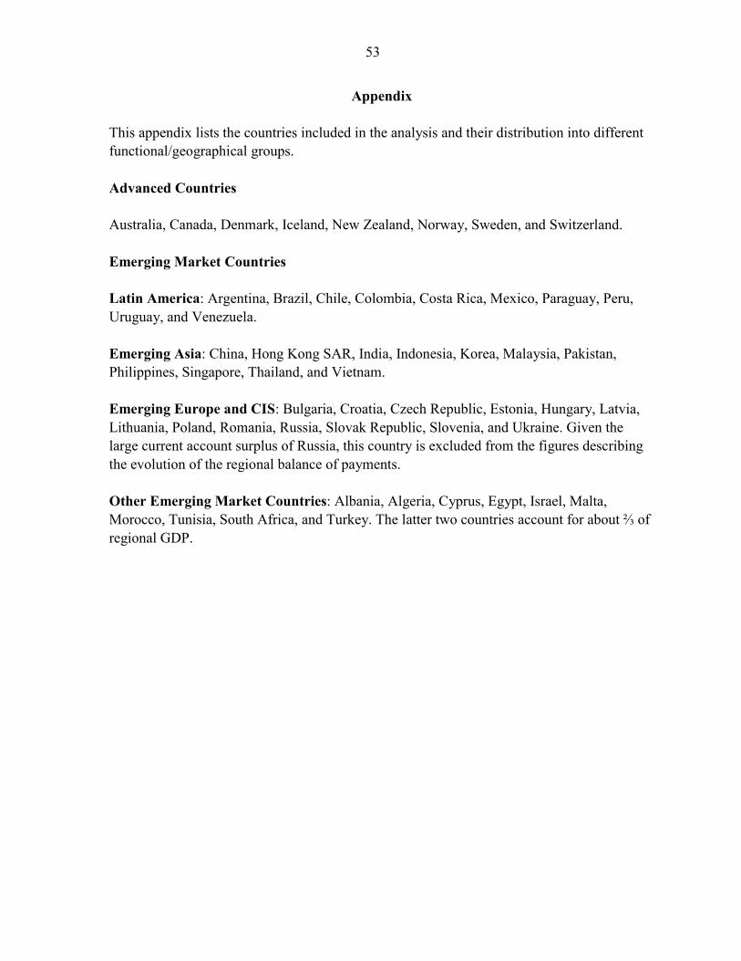
53

Appendix This appendix lists the countries included in the analysis and their distribution into different functional/geographical groups. Advanced Countries Australia, Canada, Denmark, Iceland, New Zealand, Norway, Sweden, and Switzerland. Emerging Market Countries Latin America: Argentina, Brazil, Chile, Colombia, Costa Rica, Mexico, Paraguay, Peru, Uruguay, and Venezuela. Emerging Asia: China, Hong Kong SAR, India, Indonesia, Korea, Malaysia, Pakistan, Philippines, Singapore, Thailand, and Vietnam. Emerging Europe and CIS: Bulgaria, Croatia, Czech Republic, Estonia, Hungary, Latvia, Lithuania, Poland, Romania, Russia, Slovak Republic, Slovenia, and Ukraine. Given the large current account surplus of Russia, this country is excluded from the figures describing the evolution of the regional balance of payments. Other Emerging Market Countries: Albania, Algeria, Cyprus, Egypt, Israel, Malta, Morocco, Tunisia, South Africa, and Turkey. The latter two countries account for about ⅔ of regional GDP.

54

References Ariyoshi, A., K. Habermeier, B. Laurens, I. Otker-Robe, J. Canales-Kriljenko, and

A. Kirilenko, 2000, Capital Controls: Country Experiences with Their Use and Liberalization, IMF Occasional Paper No. 190 (Washington: International Monetary Fund).

Baig, T., 2001, “Characterizing Exchange Rate Regimes in Post-Crisis East Asia,” IMF

Working Paper 01/152 (Washington: International Monetary Fund). Bartolini, L., and A. Drazen, 1997, “Capital-Account Liberalization as a Signal,” American

Economic Review, Vol. 87, No. 1 (March), pp. 138–54. Bayoumi, T., and B. Eichengreen, 1998, “Exchange Rate Volatility and Intervention:

Implications of the Theory of Optimum Currency Areas,” Journal of International Economics, Vol. 45, pp. 191–209.

Braun, M., 2001, “Why is Fiscal Policy Procyclical in Developing Countries?” Mimeo.

(Cambridge, Massachusetts: Harvard University). Bertoli, S., G. M. Gallo, and G. Ricchiuti, 2006, “Exchange Market Pressure: Some Caveats

in Empirical Applications,” Working Paper 2006/17 (Florence, Italy: Dipartimento di Statistica “Giuseppe Parenti”).

Calderon, C., and K. Schmidt-Hebbel, 2003, “Macroeconomic Policies and Performance in

Latin America,” Journal of International Money and Finance, Vol. 22, pp. 895–923. Calvo, G. A., L. Leiderman, and C. M. Reinhart, 1993 “Capital Inflows and Real Exchange

Rate Appreciation in Latin America: The Role of External Factors,” IMF Staff Papers, Vol. 40 No. 1, 108–51.

———, 1994, “The Capital Inflows Problem: Concepts and Issues,” Contemporary

Economic Policy, Vol. XII No. 3 (July), 54–66. ———, 1996, “Inflows of Capital to Developing Countries in the 1990s,” Journal of

Economic Perspectives, Vol. 10 (Spring), 123–39. Calvo, G. A., and C. A. Vegh, 1999, “Inflation Stabilization and Balance of Payment Crises

in Developing Countries,” in Handbook of Macroeconomics, Ed. 1, Vol. 1, pp. 1531-614, ed. by J. B. Taylor and M. Woodford (Elsevier).

55

Calvo, G. A., and C. M. Reinhart, 2002, “Fear of Floating,” Quarterly Journal of Economics, Vol. 117, No. 2, pp. 379–408.

Carlson, M., and L. Hernandez, 2002, “Determinants and Repercussions of the Composition

of Capital Inflows,” International Finance Discussion Papers, No. 2002–717 (Washington: Board of Governors, The Federal Reserve Board).

Cavoli, T., and R. S. Rajan, 2006, “Capital Inflows Problem in Selected Asian Economies in

the 1990s Revisited: The Role of Monetary Sterilization,” Asian Economic Journal Vol. 20, No. 4, pp. 409–23.

Chinn, M., and H. Ito, 2005, “What Matters for Financial Development? Capital Controls,

Institutions and Interactions,” forthcoming in Journal of Development Economics. Christensen, J., 2004, “Capital Inflows, Sterilization, and Commercial Bank Speculation: The

Case of the Czech Republic in the Mid-1990s,” IMF Working Paper 04/218 (Washington: International Monetary Fund).

Conover, W.J., 1980, Practical Nonparametric Statistics, Second Edition (New York: John

Wiley and Sons). Cowan, K, and J. De Gregorio, 2005, “International Borrowing, Capital Controls, and the

Exchange Rate Lessons from Chile,” NBER Working Paper No. 11382 (Cambridge, Massachusetts: National Bureau of Economic Research).

Desai, M., C. F. Foley, and J. R. Hines Jr., 2004, “Capital Controls, Liberalizations and

Foreign Direct Investment,” NBER Working Paper No. 10337 (Cambridge, Massachusetts: National Bureau of Economic Research).

Dixon, J., 2003, “Voracity, Volatility, and Growth,” Mimeo (Los Angeles, California:

UCLA). Driver, R., P. Sinclair, and C. Thoenissen, 2005, Exchange Rate, Capital Flows and Policy,

Routledge International Studies in Money and Banking (London and New York: Routledge)

Eichengreen, B., A. K. Rose, and Charles Wyplosz, 1996, “Contagious Currency Crises,”

NBER Working Paper No. 5681 (Cambridge, Massachusetts: National Bureau of Economic Research).

56

Edwards, S., 2000, Capital Flows and the Emerging Economies: Theory, Evidence, and Controversies, National Bureau of Economic Research Conference (Chicago, Illinois: The University of Chicago Press).

———, 2005, “Capital Controls, Sudden Stops, and Current Account Reversals,” NBER

Working Paper No. 11170 (Cambridge, Massachusetts: National Bureau of Economic Research).

———, 2007, “On Current Account Surpluses and the Correction of Global Imbalances,”

NBER Working Paper No. 12904 (Cambridge, Massachusetts: National Bureau of Economic Research).

———, 2007, Capital Controls and Capital Flows in Emerging Economies: Policies,

Practices and Consequences, National Bureau of Economic Research Conference (Chicago, Illinois: The University of Chicago Press).

———, and R. Rigobon, 2005, “Capital Controls, Exchange Rate Volatility and External

Vulnerability,” NBER Working Paper No. 11434 (Cambridge, Massachusetts: National Bureau of Economic Research).

Fama, E. F., L. Fisher, M. C. Jensen, and R. Roll, 1969, “The adjustment of stock prices to

new information,” International Economic Review, Vol. 10, No. 1 (February), pp. 1-21.

Fernandez-Arias, E., and P. J. Montiel, 1996, “The Surge in Capital Inflows to Developing

Countries: An Overview,” World Bank Economic Review, Vol.10, No.1, pp. 51–77 (Washington: The World Bank).

Forbes, K., 2005, “The Microeconomic Evidence on Capital Controls: No Free Lunch,”

NBER Working Paper No. 11372 (Cambridge, Massachusetts: National Bureau of Economic Research).

Frankel, J., and A. Rose, 1996, “Currency Crashes in Emerging Markets: An Empirical

Treatment,” Journal of International Economics, Vol. 41, No. 3/4, pp. 351–66. Freund, C., 2005, “Current account adjustment in industrial countries,” Journal of

International Money and Finance, Vol. 24, Issue 8 (December), pp. 1278–98. Gavin, M., and R. Perotti, 1997, “Fiscal Policy in Latin America,” NBER Macroeconomics

Annual, pp. 11–61 (Cambridge, Massachusetts: MIT Press).

57

Gibbons, M., R., 1987, “The Interrelations of Finance and Economics: Empirical Perspectives,” American Economic Review Papers and Proceedings, Vol. 77, No. 2, pp. 35–41.

Girton, L., and D. Roper, 1977, “A Monetary Model of Exchange Market Pressure Applied

to the Postwar Canadian Experience,” American Economic Review, Vol. 67, No. 4, pp. 537–48.

Glick, R., P. Kretzmer, and C. Wihlborg, 1995, “Real Exchange Rate Effects of Monetary

Disturbances Under Different Degrees of Exchange Rate Flexibility: An Empirical Analysis,” Journal of International Economics, Vol. 38, pp. 249–73.

Glick, R., and C. Wihlborg, 1997, “Exchange Rate Regimes and International Trade,” in

International Trade and Finance: New Frontiers for Research, ed. by Cohen, B. (Cambridge: Cambridge University Press).

Glick, R., ed., 1998, Managing Capital Flows and Exchange Rates: Perspectives from the

Pacific Basin (Cambridge, Massachusetts: Cambridge University Press). Glick, R., Xu. Guo, and M. Hutchison, 2006, “Currency Crises, Capital Account

Liberalization, and Selection Bias,” forthcoming in Review of Economics and Statistics.

Goldfajn, I., and A. Minella, 2005, “Capital Flows and Controls in Brazil: What Have We

Learned?” NBER Working Paper No. 11640 (Cambridge, Massachusetts: National Bureau of Economic Research).

Gourinchas, P., R. Valdes, and O. Landerretche, 2001, “Lending Booms: Latin America and

the World,” Economia, Vol. 1, No. 2 (Spring). Grilli, V., and G. M. Milesi-Ferretti, 1995, “Economic Effects and Structural Determinants of

Capital Controls,” IMF Staff Papers, Vol. 42, No. 3, pp. 517–51 (Washington: International Monetary Fund).

Hodrick, R., and E. C. Prescott, 1997, “Postwar U.S. Business Cycles: An Empirical

Investigation,” Journal of Money, Credit, and Banking, Vol. 29, No. 1 (February), pp. 1–16.

Kaminsky, G., C. M. Reinhart, and C. A. Végh, 2004, “When It Rains, It Pours: Procyclical

Capital Flows and Policies,” in NBER Macroeconomics Annual 2004, pp. 11–53, ed. by Mark Gertler and Kenneth S. Rogoff (Cambridge, Massachusetts: MIT Press).

58

Kahler, M., 1998, Capital Flows and Financial Crisis, A Council on Foreign Relations Book (Ithace, New York: Cornell University Press).

Kose, M. A., E. S. Prasad, K. Rogoff, S. J. Wie, 2009, “Financial Globalization: A

Reappraisal,” forthcoming in IMF Staff Papers. Kwack, S. Y., 2003, “An Empirical Assessment of Monetary Policy Responses to Capital

Inflows in East Asia before the Crisis,” International Economic Journal, Vol. 15, pp. 95–113.

Lane, P., 2003, “The Cyclical Behavior of Fiscal Policy: Evidence from the OECD,” Journal

of Public Economics, Vol. 86, pp. 2661–75. Levy Yeyati, E., and F. Sturzenegger, 2005, “Classifying Exchange Rate Regimes: Deeds vs.

Words,” European Economic Review, Vol. 49, No. 6 (August), pp. 1603–35. Lipschitz, L., T. D. Lane, and A. Mourmouras, 2002, “Capital Flows to Transition

Economies: Master or Servant,” IMF Working Paper 02/11 (Washington: International Monetary Fund).

Magud, N. and C. Reinhart, 2007, “Some Lessons for Policy Makers Who Deal With the

Mixed Blessing of Capital Inflows,” in Capital Controls and Capital Flows in Emerging Economies, ed. by Sebastian Edwards, 645–74 (Chicago, Illinois: The University of Chicago Press).

Mann, H.B., and D.R. Whitney, 1947, “On a Test of Whether One of Two Random Variables

is Stochastically Larger Than the Other,” Annals of Mathematical Statistics, Vol. 18, pp. 50–60.

Milesi-Ferreti, G. M., and A. Razin, 1998, “Sharp Reductions in Current Account Deficits:

An Empirical Analysis,” European Economic Review, Vol. 42 (April), pp. 897–908. Miniane, J. 2004, “A New Set of Measures on Capital Account Restrictions,” IMF Staff

Papers, Vol. 51, No. 2, pp. 276–308 (Washington: International Monetary Fund). Mody, A., and A. P. Murshid, 2005, “Growing Up With Capital Flows,” Journal of

International Economics, Vol. 65, No. 1 (January), pp. 249–66. Moreno, R., 1996, “Intervention, Sterilization, and Monetary Control in Korea and Taiwan,”

FRBSF Economic Review, Federal Reserve Board of San Franciso, Vol. 3, pp. 23–33.

59

Mauro, P., and T. Becker, 2006, “Output Drops and the Shocks That Matter,” IMF Working Paper 06/172 (Washington: International Monetary Fund).

Montiel, P. J., 1999, “Policy Responses to Volatile Capital Flows,” unpublished. Available

via the Internet: www.worldbank.org/research/interest/confs/past/paps15-16/montiel2.pdf.

———, and C. M. Reinhart, 1999, “Do Capital Controls and Macroeconomic Policies

Influence the Volume and Composition of Capital Flows? Evidence From the 1990s,” Journal of International Money and Finance, Vol. 18, No. 4 (August), pp. 619–635.

Obstfeld, M., 2009, “International Finance and Growth in Developing Countries: What Have

We Learned?” Forthcoming in IMF Staff Papers. ———, and A. Taylor, 2002, “Globalization and Capital Markets,” NBER, Working Paper

No. 8846 (Cambridge, Massachusetts: National Bureau of Economic Research). Ouyang, A. Y., R. S. Rajan, and T. D. Willet, 2007, “China as a Reserve Sink: The Evidence

from Offset and Sterilization Coefficients,” HKIMR Working Paper No. 10/2007 (Hong Kong SAR: Hong Kong Institute for Monetary Research.

Pentecost, E. J., C. Van Hooydonk, and A. Van Poeck, 2001, “Measuring and Estimating

Exchange Market Pressure in the EU,” Journal of International Money and Finance, Vol.20, pp.401–18.

Quinn, D., 1997, “The Correlates of Changes in International Financial Regulation,”

American Political Science Review, Vol. 91 (September), pp. 531–51. Rodrik, D., and A. Subramanian, 2008, “Why Did Financial Globalization Disappoint?”

Manuscript, Harvard University. Forthcoming in IMF Staff Papers. Reinhart, C. M., and V. Reinhart, 1998, “Some Lessons for Policymakers Who Deal With the

Mixed Blessing of Capital Inflows,” in Capital Flows and Financial Crises, pp. 93-127, ed. by Miles Kahler (Ithaca, New York: Cornell University Press).

———, 2008, “Capital Flow Bonanzas: An Encompassing View of the Past and Present,”

NBER Working Paper No. 14321 (Cambridge, Massachusetts: National Bureau of Economic Research).

Reinhart, C. M. and K. S. Rogoff, 2004, “The Modern History of Exchange Rate

Arrangements: A Reinterpretation,” Quarterly Journal of Economics, Vol. 119, No. 1, pp. 1–48.

60

Reinhart, C. M and K. S. Smith, 1997, “Too Much of a Good Thing: The Macroeconomic Effects of Taxing Capital Inflows,” Mimeo (Maryland: Department of Economics, University of Maryland, College Park).

Schindler, M., 2009, “Measuring Financial Integration: A New Dataset,” forthcoming in IMF

Staff Papers. Straetmans, S. T. M., R. Versteeg, and C. P. Wolff, 2008, “Are Capital Controls in the

Foreign Exchange Market Effective?” Working Paper (Netherlands: Maastricht University).

Takagi, S. and T. Esaka, 1999, “Sterilization and the Capital Inflow Problem in East Asia,”

Discussion Paper No. 86 (Tokyo: Economic Planning Agency). Van Poeck, A., J. Vanneste, and M. Veiner, 2007, “Exchange Rate Regimes and Exchange

Market Pressure in the New EU Member States,” Journal of Common Market Studies, Vol. 45, No.l 2, pp. 459–85.

Wei, S.-J., and Z. Zhang, 2006, “Collateral Damage: Exchange Controls and International

Trade,” IMF Working Paper 07/08 (Washington: International Monetary Fund). Wilcoxon, F., 1945, “Individual Comparisons by Ranking Methods,” Biometrics Bulletin,

Vol. 1, pp. 80–83. World Bank, 1997, Private Capital Flows to Developing Countries: The Road to Financial

Integration (New York: Oxford University Press).