Markovian Optimal Taxation: The Macroeconomic

Implications of Two Notions of Time Consistency

Salvador Ortigueira∗

Department of Economics

European University Institute

January 24, 2003

Abstract

In this paper we study optimal taxation in a dynamic game played by a sequence

of governments, one for each time period, and a private sector composed of a con-

tinuum of households. We focus on the Markov-perfect equilibrium of this game

under two assumptions on the extent of government’s intra-period commitment,

which in turn define two notions of time consistency of the Markov policy. Our re-

sults show that the extent of government’s intra-period commitment has important

quantitative implications for policies, welfare, and macroeconomic variables, and

consequently that it must be explicitly stated as one of the givens of the economy,

alongside preferences, markets and technology. We see this as an important result,

since most of the previous literature on Markovian optimal taxation has assumed, ei-

ther interchangeably or unnoticeably, different degrees of government’s intra-period

commitment.

Keywords: Markov-Perfect Optimal Taxation; Time-Consistent Policies; Instantaneous

and Non-Instantaneous Commitment; Numerical Methods.

JEL Classification Numbers: E61; E62.

∗I am grateful to Andrei Baliakin and Vladimir Petkov for their valuable suggestions. Address: Villa

San Paolo, Via della Piazzuola 43, 50133 Florence, Italy. E-mail: Salvador.Ortigueira@IUE.it.

1

1 Introduction

This paper analyzes optimal fiscal policy in a simple extension of the neoclassical

model of capital accumulation. Since we will be assuming that the government is unable

to commit to future policies, the Ramsey equilibrium becomes an invalid equilibrium

concept in our framework as it delivers time-inconsistent policies. Instead, we study the

Markov-perfect equilibria of a dynamic game played by a sequence of governments, one

for each time period, and the private sector, under two alternative assumptions on the

within-period timing of actions, which define two notions of time consistency. Our main

aim is to understand and quantify the effects of these two timings on the Markov-perfect

equilibrium of this game.

As noticed by Cohen and Michell (1988), the literature on Markovian optimal policies

has made use of two notions of time consistency involving different timings of actions

supported by different degrees of government’s intra-period commitment. And, more

importantly, they also note that the two notions have been used either interchangeably or

unnoticeably, thus hindering the assessment of the results. Under the first notion of time

consistency, which we call here genuinely time consistent, both the private sector and the

current government choose their actions simultaneously. Hence, the government does not

need to express any commitment to its policy since there is no time lag between the tax

and the consumption decisions. This notion of time consistency bears the strongest sense

of lack of commitment. Under the second notion, which we call quasi time consistent, the

current government moves first to set taxes before the household chooses consumption.

This allows the government to anticipate the private sector’s response to taxes, which

confers the government with instantaneous leadership. As a consequence, intra-period or

instantaneous commitment is needed, so that the private sector will not expect a change

in taxes after consumption has been decided. This second notion of time consistency

bears a weaker sense of lack of commitment.

Analyses of Markovian optimal taxes where one or the other of these notions of time

consistency is adopted abound in the literature: Turnovsky and Brock (1980) and Judd

(1998, Ch. 16) present a simple model with valued government expenditure, and derive

Markovian optimal taxes under the assumption that the government and the private sec-

tor move simultaneously (genuinely-time-consistent taxes). Klein, Rıos-Rull and Krusell

2

(2003) study optimal taxes in a similar model, assuming that the government moves first

(quasi-time-consistent taxes).

However, the extent to which the choice of the timing of actions affects the level of

optimal taxes and other macroeconomic variables is not well understood. Even though

the distinction between the two scenarios is subtle, there is no reason to believe that it

has only negligible effects on welfare and on macroeconomic variables. In this paper we

ask the following questions: How do Markovian optimal taxes change with the timing

of actions? Does the government attain higher welfare when granted with instantaneous

commitment, and moves first? Are the effects of the timing of actions quantitatively

important? The only attempt we are aware of to answer these questions is in Cohen

and Michell (1988). Although their analysis sheds new light on how to calculate time-

consistent policies, it presents some limitations to address the above-mentioned questions.

First, their model is not a fully-fledged macroeconomic model. Second, they assume a

quadratic loss function and a linear law of motion for the state variable, so that the model

can be solved analytically. As is well known, deviations from the linear-quadratic structure

typically break up the possibility of analytical solutions, and leave numerical methods

as the only resource to find solutions. For reasons that will become clear below, the

application of numerical methods in this type of models is not a straightforward endeavor,

and even in simple, one-sector economies such as the one studied in this paper computing

numerical solutions poses a number of challenges, especially for the case of quasi-time-

consistent Markovian optimal policies. This latter type of policy is the focus in Klein,

Krusell and Rıos-Rull (2003), but they only compute steady-state values. Thus, their

numerical approach not only falls short in providing a full description of the equilibrium

solution, but also leaves unanswered important questions about the properties of the

computed stationary values. One of these questions is related to the stability of such

steady state. Since in dynamic games with a continuum of players the uniqueness of the

equilibrium is not guaranteed, a check of stability seems to be mandatory before drawing

any conclusions from the computed stationary values.

In this paper we answer the questions posed above within the context of a neoclassical

model of capital accumulation that includes valued government expenditure and income

taxation. This model is completely standard in the recent literature of optimal taxation

[see Judd (1998, Ch. 16), Klein, Rıos-Rull and Krusell (2003) for an analysis of Markovian

3

optimal taxation, and Phelan and Stachetti (2001) for an analysis of optimal taxation

under sequential equilibria]. Our main result is that the timing of actions within a time

period has sizable quantitative implications both in terms of tax rates and welfare in a

Markov-perfect equilibrium. For our benchmark economy, tax rates on total income in a

Markov equilibrium with simultaneous moves (genuinely-time-consistent taxes) are half

the tax rates in a Markov equilibrium with government’s instantaneous leadership (quasi-

time-consistent taxation). In terms of welfare, government’s leadership bears a cost of 7%

of consumption of the private good. Thus, our results unambiguously show that the timing

of actions is a key ingredient of the environment in the analysis of Markovian optimal

taxes, and that, contrary to previous studies in this area, it must be explicitly stated

alongside other ingredients such as preferences, markets and technology. Furthermore,

our analysis also sheds light on the issue of optimal fiscal constitutions. Our quantitative

exercise shows that the optimal fiscal constitution must limit the government’s ability to

commit, if the alternative is to grant intra-period commitment. A final contribution of

this paper is to show how a projection method can be applied to the computation of the

Markov-perfect equilibria in this type of models. We compute these equilibria for a wide

range of the state space, which allows us not only to derive its global properties, but also

to carry out a welfare analysis.

Projection methods [see Judd (1992),(1998) and Miranda and Fackler (2002)] are a

natural and efficient way to solve functional equation problems, and, more specifically, to

solve dynamic games. The application of these methods has proved extremely useful to

solve dynamic games arising in models of industrial organization. In a recent paper, Vede-

nov and Miranda (2001) apply a projection method to a dynamic duopoly game in which

competing firms can invest in physical capital. A similar method is applied by Miranda

and Rui (1996) to models of world commodity markets where two countries compete us-

ing strategic storage. Our model in this paper has, however, remarkable differences with

respect to models of dynamic duopoly games. On the one hand, one of our players is the

private sector which is made up of a continuum of households, and “plays” through the

market. On the other hand, we cannot assume symmetric strategies as is usually done in

duopoly games.

The paper is organized as follows. Section 2 presents the model and a formal definition

of the Markov-perfect equilibrium under both notions of time consistency. In Section 3

4

the model is parameterized and calibrated, and the equilibria are computed. Section 4

presents an extension of the model with endogenous leisure-labor choice. The Markov-

perfect equilibrium is presented, and the macroeconomic and welfare consequences of the

timing of actions are discussed. Section 5 presents our computational approach, Section

6 concludes, and Section 7 contains the Appendix.

2 The Model and Equilibrium Definitions

In this section we present a simple model of capital accumulation with valued govern-

ment expenditure. The government uses taxes on total income to finance its expenditures.

Households

There is a measure one of identical households. Household’s lifetime utility is given

by∞X�=0

���(��� ��)� (2.1)

where �� denotes the level of private-good consumption, and �� is the level of public-good

consumption. The instantaneous utility function, � , is assumed to be increasing in both

arguments, jointly concave and continuously differentiable. The household supplies one

unit of labor time inelastically, whereby it receives a wage rate ��. It also owns a stock

of capital, ��, which rents at a rate ��, and whose rate of depreciation is denoted by

0 1. Total income is subject to taxation. The household’s budget constraint, in

combination with the law of motion for capital, yields,

�� + ��+1 = �� + (1− ��)[�� + (�� − )��]� (2.2)

where �� is the tax rate on total income net of capital depreciation.

The Firms’ Sector

The firms’ sector employs capital and labor to produce the aggregate good. Total

production is given by,

� = � (��� 1) = �(��)� (2.3)

where �� is the aggregate stock of capital, and � is a neoclassical production function.

Firms are competitive, and therefore,

�� = ��(��)� (2.4)

5

�� = �(��)− ����� (2.5)

Government

The government is assumed to run a balanced budget, which implies that at every

period total expenditure must equal total income from taxes,

�� = ��[�� + (�� − )��] = ��[�(��)− ��]� (2.6)

where the second equality follows from the zero-profit condition in the firms’ sector.

2.1 Markovian Optimal Taxation

When the government lacks the ability to commit to future policies, the Ramsey solu-

tion becomes a less interesting equilibrium concept, since it is time inconsistent. Among

all equilibrium concepts delivering time-consistent policies, the Markov-perfect equilib-

rium stands out for a number of reasons, such as the simplicity with which it embeds

rational behavior, or its power to enhance the model’s predictability by yielding a lower

number of equilibria than alternative equilibrium concepts1. In contrast to the Ramsey

equilibrium, the government is now assumed to act sequentially. Thus, we can think of

a sequence of governments, each foreseeing how its successors will behave, that chooses

the tax rate on total income, conditioning on the aggregate stock of capital, to maximize

social welfare. Finally, and before moving to the characterization of the Markov-Perfect

equilibria under the two timings of actions described above, we want to notice that our

analysis will be restricted to the case of differentiable Markovian strategies. This is a

standard restriction in the literature of Markovian optimal taxation2.

2.1.1 Genuinely-Time-Consistent Markovian Optimal Taxes

In this section we characterize genuinely time consistent Markovian optimal taxes. The

period � government, and households choose their actions simultaneously. Each household

1For a more detailed discussion of the virtues of the Markov-Perfect equilibrium see Maskin and Tirole

(2001).2It has been recently shown [see Sorger (1998) for an application to resource games, and Krusell and

Smith (2003) for an application to models with quasi-geometric discounting] that the Markov-Perfect

equilibrium may be indeterminate if continuity and differentiability are not imposed.

6

decides how much to consume and save given its stock of capital, the economy-wide stock

of capital, and the expected tax policy for the current and future governments. The

current government chooses the tax rate for the current period given the economy-wide

stock of capital and the expected tax policy of future governments. Before providing a

definition of a genuinely-time-consistent Markovian equilibrium, let us present the problem

of a household, and of the current government in more detail.

The problem of the household

Let � denote the household’s stock of capital, and� the economy-wide stock of capital.

If the household expect that the current and future governments will set taxes according

to the policy �, where � is a function that maps the economy-wide stock of capital into

a tax rate on total income, its maximization problem can be compactly written as,

�(���;�) = ������0½�(�� �) + ��(�0� � 0;�)

¾� (2.7)

subject to the budget constraint,

�+ �0 = � + (1− �(�))[�(�) + (�(�)− )�]� (2.8)

where the economy-wide stock of capital is expected to evolve according to the law, say,

� 0 = �(�). In (2.7), �(���;�) is the value for a household with a stock of capital �,

when economy-wide capital is �, and the tax policy is �.

It is then clear from (2.7)-(2.8) that for a given tax policy, household’s consumption

is a function of � and � alone. Furthermore, if we now use the fact that all households

are identical, � = �, the consumption function in a competitive equilibrium under the

tax policy � must satisfy the following Euler equation,

��

µ�(�)� �(�)

¶= ���

µ�(� 0)� �(� 0)

¶ ·1 + (1− �(� 0))[��(� 0)− ]

¸� (2.9)

where � 0 in equilibrium is given by,

� 0 = � + (1− �(�))[�(�)− �]− �(�)� (2.10)

and

�(�) = �(�)[�(�)− �]� (2.11)

7

The problem of the government

The government’s objective function is to maximize social welfare. The period � gov-

ernment chooses the period � tax rate, � , taking as given the tax policy followed by

future governments. Since the government and the household move simultaneously, the

government cannot anticipate the household’s response to different tax rates. The only

trade-offs in the government’s problem are the amount of the public good to provide, and

next period’s capital stock. More specifically, the problem of the period � government is,

� (�) = ����

½�µ�(�)� G(�� � )

¶+ �� (� 0)

¾� (2.12)

where,

� 0 = � + (1− � )[�(�)− �]− �(�)� (2.13)

and

G(�� � ) = � [�(�)− �]� (2.14)

Proposition 1: The tax policy that solves the government’s problem is the solution to

the following Generalized Euler Equation:

�� = �·� 0��

0� + �

0� ·µ� 0� + 1− − � 0�

¶¸� (2.15)

where a subscript denotes the variable with respect to which the derivative is taken, and a

prime indicates the function is evaluated at next-period’ values.

The proof of this proposition is presented in the Appendix. Notice that functions’ ar-

guments in (2.15) have been dropped for expositional clarity, since there is no risk of

ambiguity.

The interpretation of the Generalized Euler Equation is reminiscent of that for the

household’ Euler equation. The government will set the tax rate so that the marginal

utility of taxation equates the marginal utility of investment in physical capital. The

marginal utility of taxation is the increase in government expenditure, G� , times themarginal utility of consuming the public good, ��, per unit of investment crowded-out,

which is exactly G� since current consumption is unaffected by the current tax rate,and therefore an increase in government expenditure translate into a one-to-one drop in

investment. Hence, today’s marginal utility of taxation is ��, the left-hand side of (2.15).

Seeing that the right-hand side of equation (2.5) is the marginal utility of investing in

8

capital is equally straightforward. An extra unit of investment today brings about and

increase in tomorrow’s output of � 0� + 1 − . The break down of this increase is: (i)� 0� is in consumption of the private good, which yields � 0��

0�; (ii) G0� is in government

expenditure from the increase in the tax base, which yields � 0�G0�; and (iii) the remaining� 0� + 1− −� 0� − G 0� is in taxation, and since tomorrow’s marginal utility of taxation is� 0�, this yields �

0� · (� 0� + 1− − � 0� − G0�). Adding up all these yields and discounting,

gives the right-hand side of the Generalized Euler Equation.

We can now define a Markov-perfect equilibrium for this economy.

Definition: A genuinely-time-consistent Markov equilibrium (GTCE) is a triple of func-

tions �(�), �(�) and � (�), such that: (i) �(�) solves the first-order condition of the

household sector [eqs. (2.9)-(2.11)]; (ii) �(�) solves the Euler equation of the govern-

ment [eqs. (2.13)-(2.15)]; and (iii) � (�) is the value function of the government, that is,

� (�) = � [�(�)�G(���(�))] + �� (� 0)�

2.1.2 Quasi-Time-Consistent Markovian Optimal Taxes

The period � government is now assumed to have instantaneous leadership in the

sense that it sets the period � tax rate before the household decides on consumption and

savings. Thus, when choosing among feasible tax rates, the government is able to asses

the household’s response to such taxes.

The problem of the household

When the household decides on consumption and savings, the period � government has

already set the period � tax rate. Then, the problem of a household with � units of capital

that has to pay taxes on current income at rate � , and that expects future governments

to follow the tax policy �, is

�(���; �) = ������0½�(�� �) + ��(�0� � 0; �)

¾� (2.16)

subject to the budget constraint,

�+ �0 = � + (1− � )[�(�) + (�(�)− )�]� (2.17)

where the economy-wide stock of capital is expected to evolve according to the law, say,

� 0 = H(�).

9

It thus follows from (2.16)-(2.17) that household’s consumption is a function of �,

� and � . Furthermore, using the representative household assumption, � = �, the

consumption function in a competitive equilibrium when today’s tax rate is � , and future

taxes are given by policy �, must satisfy the following Euler equation,

��

µC(�� �)� G(�� � )

¶= ���

µC(� 0� � 0)� G(� 0� � 0)

¶ ·1 + (1− � 0)[��(� 0)− ]

¸� (2.18)

where � 0 = �(� 0), and � 0 in equilibrium is given by,

� 0 = � + (1− �)[�(�)− �]− C(�� � )� (2.19)

and,

G(�� � ) = � [�(�)− �]� (2.20)

The problem of the government

As in the genuinely-time-consistent equilibrium, the current government chooses the

current tax rate, � , taking as given the tax policy followed by future governments. Now,

however, government’s leadership implies that it must internalize the effects of � on the

level of consumption as given by the consumption function that solves (2.18). More

specifically, the problem of the government is,

V(�) = ��� �

½�µC(�� � )� G(�� � )

¶+ V(� 0)

¾(2.21)

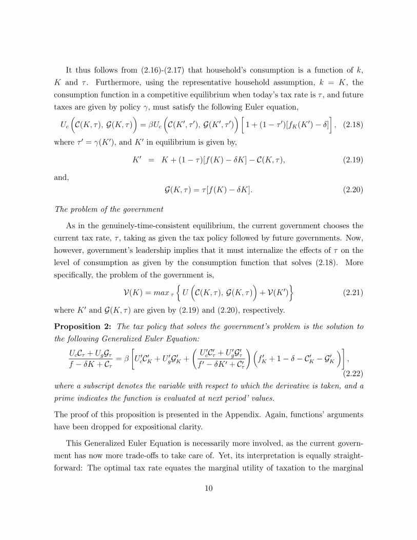
where � 0 and G(�� � ) are given by (2.19) and (2.20), respectively.Proposition 2: The tax policy that solves the government’s problem is the solution to

the following Generalized Euler Equation:

��C� + ��G�� − � + C� = �

"� 0�C0� + � 0�G0� +

Ã� 0�C0� + � 0�G0�� 0 − � 0 + C0�

!µ� 0� + 1− − C0� − G0�

¶#�

(2.22)

where a subscript denotes the variable with respect to which the derivative is taken, and a

prime indicates the function is evaluated at next period’ values.

The proof of this proposition is presented in the Appendix. Again, functions’ arguments

have been dropped for expositional clarity.

This Generalized Euler Equation is necessarily more involved, as the current govern-

ment has now more trade-offs to take care of. Yet, its interpretation is equally straight-

forward: The optimal tax rate equates the marginal utility of taxation to the marginal

10

utility of investing in capital. The only difference with respect to the case of genuinely-

time-consistent taxes relies in the determination of the marginal utility of taxation. Now,

current consumption changes with current taxes, and the increase in government expen-

diture does not imply a one-to-one decrease in investment.

The left-hand side of (2.22) is today’s marginal utility of taxation, which is made up

of three values: the change in utility from the consumption of the private good, ��C� ,the change in utility from the consumption of the public good, ��G� , and the lost ininvestment, � − � + C� . That is, the marginal value of taxation is the net gain in utilityper unit of investment crowded-out. The right-hand side of (2.22) is the marginal utility

of investing in capital. An extra unit of investment today brings about and increase in

tomorrow’s output of � 0� + 1− , whose break down is: (i) � 0� is in consumption of the

private good, which yields � 0��0� ; (ii) G0� is in government expenditure from the increase

in the tax base, which yields � 0�G0�; and (iii) the remaining � 0� + 1 − − � 0� − G0� is in

taxation, whose marginal utility has been calculated above. Adding up all these yields

and discounting, gives the right-hand side of the Generalized Euler Equation.

We define now a quasi-time-consistent Markov equilibrium for this economy.

Definition: A quasi-time-consistent Markov equilibrium (QTCE) is a triple of functions

C(�� �), �(�) and V(�), such that: (i) C(�� �) solves the first-order condition of thehousehold sector [eqs. (2.18)-(2.20)]; (ii) �(�) solves the Euler equation of the government

[eqs. (2.19), (2.20) and (2.22)]; and (iii) V(�) is the value function of the government,that is, V(�) = � [C(�� �(�))�G(�� �(�))] + �V(� 0)�

Before closing this section, and since we will present the welfare and macroeconomic

implications of the two notions of time consistency in the next, we find it convenient

to briefly introduce here the efficient equilibrium with lump-sum taxes (LSTE). Under

lump-sum taxes, the household’s Euler equation is undistorted, and the government will

set taxes so that the marginal utility of consuming the public good equals the marginal

utility of consuming the private good. That is, in the efficient equilibrium with lump-sum

taxes, the Generalized Euler Equation is replaced by the condition �� = ���

11

3 Welfare and Macroeconomic Implications

In this section we parameterize our economic model, assign values to its parame-

ters, and compute the equilibria defined above: The two Markov equilibria, GTCE and

QTCE; and the equilibrium with lump-sum taxes, LSTE. Then, we present and discuss

the welfare and macroeconomic effects of the two timings of actions embedded in those

two Markov equilibrium definitions. The functional forms for the production technology

and preferences are the standard Cobb-Douglas production function, and the CES utility

function, respectively. If we use � to denote the capital’s share of income, the production

function is,

�(��) = ���� (3.1)

where � 0 is a constant. Likewise, if we use 1!" to denote the elasticity of intertemporal

substitution of the composite good ���� , the instantaneous utility function is,

#(��� ��) =

³���

�

´1− − 11− " (3.2)

where $ 0 is a constant. In the limiting case where " = 1, this function is %&� ��+$ %&� ���

Regarding parameter values, we choose our benchmark economy as follows: The values

for � and " are arbitrarily set at 1; the value for � is set at 0.36, which is the capital’s

share of income in the US economy; is set at 0.09; the value for � is 0.96; finally, the

value for $ is set at 0.2 so that government spending as a share of income falls within the

range 15-25 per cent under both notions of time consistency. We will conduct a sensitivity

analysis with respect to " by also considering " = 5 and " = 10. Thus, our benchmark

economy is:

� = " = 1� � = 0�36� = 0�09� � = 0�96� and $ = 0�2�

The numerical approach to compute the Markov-perfect equilibria is explained in detail

in Section 5. As we have already advanced in the introductory section, our approach is

a version of a standard projection method with Chebyshev polynomials. Our computa-

tions are confined to values of the capital stock in the interval [3�75� 5�2], which contains

the steady-state capital stocks of the GTCE, QTCE, and the efficient equilibrium with

lump-sum taxes. The interval is sufficiently large to capture the global properties of the

equilibria along the transitional dynamics, and small enough so that arbitrarily low com-

12

putational errors can be attained without having to resort to “too” high-order Chebyshev

polynomials.

The results of our exercise in this section are presented in figures 1 to 4. Figure 1

presents net savings, tax policies, and consumption of the private and public goods in the

GTCE, QTCE, and the efficient equilibrium with lump-sum taxes. For our benchmark

economy, both tax policies, �(�) and �(�), are increasing functions of�, and taxes in the

QTCE are roughly 65% higher than those in the GTCE. Higher taxes translate into lower

savings, lower consumption of the private good, and higher consumption of the public

good. The steady-state capital stock in the QTCE is 4.2, while in the GTCE is 4.4. Both

steady-state capital stocks are below the level of the efficient equilibrium with lump-sum

taxes. Figure 2 plots the residuals of Chebyshev collocation for the Euler Equation, the

Generalized Euler Equation, and the Bellman Equation in the three computed equilibria:

GTCE, QTCE, and LSTE.

In Figures 3 and 4 we present the results of the sensitivity analysis with respect to ".

Figure 3 displays the GTCE for " = 1, " = 5 and " = 10. The effects of increases in " are

the expected ones. As the elasticity of intertemporal substitution, 1!", decreases, the tax

policy and consumption become flatter with respect to �. The steady-state capital stock

is, however, insensitive with respect to ". Figure 4 depicts the QTCE for the three values

of ". The results in terms of consumption and steady-state capital are qualitatively

the same as those in the GTEC. Regarding the tax policy, taxes shift upwards in the

considered state space, but are relatively less sensitive to increases in ", as compared to

the GTEC.

We can sum up our results about the effects of the timing of actions on equilibrium

outcomes by way of comparison with the efficient equilibrium with lump-sum taxes. If

the government is endowed with instantaneous commitment (moves first), there will be

underconsumption of the private good, and overconsumption of the public good. If the

government lacks instantaneous commitment (simultaneous moves) there will be overcon-

sumption of the private good, and underconsumption of the public good. The welfare

implications are discussed below.

Welfare Implications

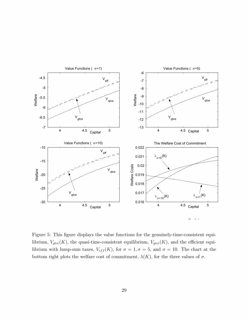
Value functions for the GTCE, QTCE and the efficient equilibrium with lump-sum

13

taxes for " = 1� " = 5, and " = 10 are plotted in Figure 5. The QTCE delivers the lowest

level of welfare. In order to provide a measure of the welfare consequences of the timing of

actions in the QTCE, we adopt an approach which has been first proposed to measure the

welfare cost of fluctuations, and then applied to measure the welfare cost of taxation. In

our model, it consists in computing the percentage increase in consumption of the private

good that would leave the representative household indifferent between the two timings of

actions. Since we do not restrict the initial capital stock, the welfare cost of endowing the

government with instantaneous commitment can be expressed as the following function

of �,

'(�) =

Ã1 + (1− �)(1− ")� (�)1 + (1− �)(1− ")V(�)

! 11−�

− 1 (3.3)

Equation (3.3) follows from equating lifetime utility under both timings of actions when

the instantaneous utility function is given by (3.2). In the limiting case where " = 1, the

welfare cost of instantaneous commitment is,

'(�) = (�)µ(1− �) [� (�)− V(�)]

¶− 1 (3.4)

In the bottom-right chart of Figure 5 we plot '(�) for the three values of "� The

welfare cost of instantaneous commitment is around 2% of consumption of the private

good, and there is no much variation with respect to the value of "� A lost of 2% of

consumption is typically considered a low welfare cost. It should be noticed, however,

that the model we used to derive this cost assumes that labor is inelastically supplied,

and therefore, it fails to comprise the effects of the timing of actions via distortions in

labor supply. In the next section we extend the model by introducing leisure in the utility

function.

4 The Model with Endogenous Labor Supply

In this section we study a more general version of the previous model with a leisure-

labor choice in the household problem. Household’s instantaneous utility is now given

by �(��� ��� %�), where %� stands for leisure, and the function � is assumed to have all the

standard properties. Production is now represented by � (��� *�), where *� denotes labor.

The normalization of the total endowment of time per period implies that %� = 1 − *�,

14

and therefore, only a new function needs to be solved for in equilibrium, which we denote

by *(�) under genuinely-time-consistent optimal taxation, and by N (�� � ) under quasi-time-consistent optimal taxation.

Genuinely-Time-Consistent Taxation

If households expect the current and future governments to set taxes according to

the tax policy �, the first-order conditions for leisure and consumption in a competitive

equilibrium under tax policy �, are, respectively,

��

µ�(�)� +(�)� �(�)

¶= ��

µ�(�)� +(�)� �(�)

¶(1− �(�))�� (��*(�))

��

µ�(�)� +(�)� �(�)

¶= ���

µ�(� 0)� +(� 0)� �(� 0)

¶×µ

1 + (1− �(� 0))[��(�0� *(� 0)− ]

¶�

where +(�) = 1−*(�), and � 0 and �(�) are given, respectively, by (2.10) and (2.11)

after substituting �(�) by � (��*(�)).

Likewise, following arguments similar to those in Section 2, the problem of the gov-

ernment yields the following Generalized Euler Equation,

�� = �·� 0��

0� − � 0�* 0

� + �0� ·µ� 0� + �

0�*

0� + 1− − � 0�

¶¸(4.1)

where, as in Section 2, we have omitted functions’ arguments, and primes mean that the

function is evaluated at next period’s values. The interpretation of this Generalized Euler

Equation is identical to the case of inelastic labor supply, and therefore, we will not repeat

it here. For the same reason, we also skip the formal definition of the Markov equilibrium

with simultaneous moves.

Quasi-Time-Consistent Taxation

Under quasi-time-consistent optimal taxation, the household’s first-order conditions

for leisure and consumption are, respectively,

��

µC(�� � )� L(�� �)�G(�� � )

¶= ��

µC(�� �)� L(�� � )�G(�� �)

¶(1− � )��(��N (�� � ))

��

µC(�� � )� L(�� �)�G(�� � )

¶= ���

µC(� 0� � 0)� L(� 0� � 0)�G(� 0� � 0)

¶×µ

1 + (1− � 0)[��(�0�N (� 0� � 0))− ]

¶�

15

where L(�� � ) = 1 − N (�� �), and � 0 = �(� 0). As before, � 0 and G(�� �) are given,respectively, by (3.19) and (2.20) after substituting �(�) by � (��N (�� � )).The government’s Euler equation is given by,

��C� − ��N� + ��G�� − � − (1− �)��N� + C� = �

·� 0�C 0� − � 0�N 0

� + �0�G 0� +

Ã� 0�C0� − � 0�N 0

� + �0�G0�

� 0 − � 0 − (1− �0)� 0�N 0� + C0�

! µ� 0� + �

0�N 0

� + 1− − G0� − C0�¶ ¸(4.2)

A Parameterized Economy with Endogenous Labor

The functional forms for the production and utility functions are the natural extensions

of the functions presented above. That is, the production function is Cobb-Douglas,

� (��� *�) = ���� *

1−�� (4.3)

where � 0, and 0 � 1 is the capital’s share of income. And instantaneous utility

is the CES function,

#(��� ��� %�) =

³���

� %

�

´1− − 11− " (4.4)

where , 0 is a constant parameter. In the limiting case where " = 1 this function is

%&� �� + $ %&� �� + , %&�%�.

We adopt the benchmark economy presented in the previous section, along with a

value for , equal to 0.2. Figures 6 and 7 show the genuinely-time-consistent, the quasi-

time-consistent and the efficient equilibrium for the benchmark economy with endogenous

labor. The results here are not qualitatively different from those in Section 3: Taxes are

higher when the government moves first, there is underconsumption of the private, un-

derinvestment, and overconsumption of the public good. When the government and the

private sector move simultaneously, there is overconsumption of private good, underin-

vestment, and underconsumption of the private good. Regarding the new endogenous

variable in this version of the model, labor, both Markov-perfect equilibria render under-

employment. It is clear from the top-left chart in Figure 7 that the high taxes of the

QTCE have the strongest distortionary effects on labor.

These results are, however, quantitatively very different. Here, taxes in the QTCE

are 100% higher than in the GTCE, as compared to the 65% in the model with inelastic

16

labor supply. The effects on welfare are also substantially higher in this version of the

model. The bottom-left chart in Figure 7 shows the welfare cost associated with govern-

ment’s instantaneous leadership, for all values of � in our state space. The proportion of

consumption of the private good that the representative household gives up ranges now

from 6�7% to 7%.

5 Numerical Strategy

In this section we present the strategy adopted for the computation of the Markov

equilibria. We restrict the discussion to the case of quasi-time-consistent taxes, since the

computation of genuinely time-consistent taxes is substantially simpler, and it can be

easily formulated as a particular case of the former. Also, we confine the presentation to

the model with exogenous labor.

Computation of Quasi-Time-Consistent Markov Equilibria.

We need to compute three functions, C(�� � ), �(�) and V(�), that solve the twoEuler equations (2.18)-(2.20) and (2.22), and the Bellman equation (2.21). First, we solve

for C(�� �) and �(�), and then we find V(�). We follow a standard projection methodwith Chebyshev polynomials and Chebyshev collocation. The basic idea is to approx-

imate the two unknown functions using Chebyshev polynomials, which are a basis for

the space of continuous functions, and then to compute the coefficients of the Chebyshev

polynomials so that these approximations exactly satisfy the two Euler equations at a

number of points. These latter points are the zeros of the Chebyshev polynomial whose

order is equal to the number of coefficients to be computed. Finally, and in order to verify

the quality of the approximation, we must check the errors at all points other than the

zeros of the Chebyshev polynomial. Even though the application of this method to our

problem at hand is quite straightforward, there are some specific features which need to

be embedded in this general algorithm. One of these features is the endogeneity of taxes,

which contributes to increase the non-linearity of the problem, and adds a new set of

restrictions.

The consumption function, C(�� �), is approximated by,

C(�� �� �) =�1X�=1

�2X�=1

���-��(�� �)� (5.1)

17

where the two-dimensional Chebyshev polynomials, -��(�� � ), are the tensor products of

the one-dimensional polynomials, that is, -��(�� � ) = -�−1[2(�−����)!(����−����)−1]-�−1[2(� − ����)!(���� − ����) − 1]. The one-dimensional Chebyshev polynomials areevaluated by recursion: -0(�) = 1� -1(�) = �� -�+1(�) = 2�-�(�) − -�−1(�)� Thematrix � = (���), . = 1� ���� /1; 0 = 1� ���� /2 is the matrix of unknown coefficients in

the consumption function. The values ����� ����� ���� and ���� are used to transform

the original variables, since the Chebyshev polynomials are defined in the interval [−1� 1].Notice that the election of���� and���� is free, and it simply indicates that� is confined

to the interval [���������]. We will set these two values so that the steady-state capital

stock lies within this interval. Since there is no way the steady-state equilibrium can be

known a priori, some experimentation is necessary in order to pin down an interval that

contains the steady-state capital stock. Regarding ���� and ����, it should be observed

that tax rates are endogenous, and, therefore, the election of the interval for taxes must

be consistent with the optimal rule for taxes. We will discuss this issue below.

The policy rule, �(�), is approximated by,

�(�� 1) =�3X�=1

1�-�−1[2(� −����)!(���� −����)− 1]� (5.2)

where the vector 1 = (11� ���� 1�3), is the vector of unknown coefficients in the policy rule.

The total number of coefficients to be determined is /1 × /2 + /3. These coefficientsare fixed by imposing that C(�� �� �) and �(�� 1) satisfy the two Euler equations at (/1×/2+/3)!2 collocation points. These points are the (/1×/2+/3)!2 roots of the Chebyshevpolynomial of order (/1 × /2 + /3)!2. Thus, the problem reduces to solving a system of

non-linear equations formed by the household’s Euler equation,

��

hC(��� �(��� 1)� �)� G(��� �(��� 1))

i−

���

hC(� 0

�� �(�0�� 1)� �)� G(� 0

�� �(�0�� 1))

i ³1 + (1− �(� 0

�� 1))[��(�0�)− ]

´= 0 (5.3)

and the government’s Euler equation,

��(��� �� 1)C�(��� �� 1) + ��(��� �� 1)G�(��� 1)

�(��)− �� + C� (��� �� 1)− �

½��(�

0�� �� 1)C�(� 0

�� �� 1)+

��(�0�� �� 1)G�(� 0

�� 1) +

��(�

0�� �� 1)C�(� 0

�� �� 1) + ��(�0�� �� 1)G�(� 0

�� 1)

�(� 0�)− � 0

� + C�(� 0�� �� 1)

!×

18

µ1 + (1− �(� 0

�� 1))[��(�0�)− ]− C�(� 0

�� �� 1)¶¾

= 0

(5.4)

evaluated at the collocation points ��, for . = 1� ���� (/1 × /2 + /3)!2; where � 0� is

� 0� = �� + (1− �(��� 1))

·�(��)− ��

¸− C

µ��� �(��� 1)� �

¶� (5.5)

The compact notation in (5.4) corresponds to,

��(��� �� 1) = ��

µC(��� �(��� 1)� �)� G(��� �(��� 1))

¶��(�

0�� �� 1) = ��

µC(� 0

�� �(�0�� 1)� �)� G(� 0

�� �(�0�� 1))

¶C� (��� �� 1) = C� (��� �(��� 1)� �)

C� (� 0�� �� 1) = C� (� 0

�� �(�0�� 1)� �)

�� (��� 1) = �� (��� �(��� 1))

�� (�0�� 1) = �� (�

0�� �(�

0�� 1))

for 2 = �� � and = �� � .

Since taxes are endogenous variables, we must guarantee that they lie in the interval

[����� ����]. In order to do so, we set ���� and ���� as,

���� = �./{�(��� 1)} (5.6)

���� = ���{�(��� 1)} (5.7)

The way we implement these two latter restrictions is the following: (i) we impose ���� =

�(����� 1) and ���� = �(����� 1), and then look for solutions to (5.3)-(5.5); (ii) then, we

impose ���� = �(����� 1) and ���� = �(����� 1) and look for solutions to (5.3)-(5.5); (iii)

finally, we look for Markov-perfect equilibria by imposing that the minimum or maximum

tax rates, or both, are in the interior of [���������].

One of the main difficulties in implementing the projection method is to come up

with a good initial guess for unknown coefficients so that a solution to the system of

Euler equations, evaluated at the collocation points, can be found. This is a problem

that typically arises when the system of equation is highly non-linear. In our model, the

19

problem is aggravated by the fact that taxes are endogenous. There are mainly two ways

to cope with this situation. The first one is to use the solution of degenerate cases, or

solutions of alternative, lower-quality methods as the initial the guess. The second one is

to use the solution of the least squares method, consisting in minimizing the sum of the

squared residuals, as the initial guess. This minimization problem always yield a solution,

and is extremely easy to implement.3 In this paper, we use the latter alternative to

obtain initial guesses. Some remarks are in order. Since uniqueness of the Markov-perfect

equilibrium can not be guaranteed, and since the problem of minimizing the sum of the

squared residuals can find a local minimum, some additional work is needed. What we

have done here is to use the solution of the minimization problem, and some conveniently

perturbed versions of this solution, as initial guesses. For our parameterization of the

model, and all sets of parameter values considered in this paper, we found a unique

solution to the system (5.3)-(5.5) rendering a stable equilibrium.

Finally, the computation of the value function is straightforward. Using the solutions

for C(��� �� �) and �(��� 1), the value function, V(�), is approximated by,

V(�� 3) =�4X�=1

3�-�−1[2(� −����)!(���� −����)− 1]�

where the vector 3 = (31� ���� 3�4), is the vector of unknown coefficients in the value

function. These coefficients are the solutions to the following system of /4 equations.

V(��� 3) = �·C(��� �(��� 1)� �)� G(��� �(��� 1))

¸+ V(� 0

�)

at the collocation points �1� ������4 , and where �0�, for . = 1� ���� /4, are given by equation

(5.5).

6 Conclusions

Since the seminal paper by Kydland and Prescott (1977), several authors have followed

different strategies to characterize time-consistent optimal fiscal policies. In this paper

we have studied Markovian optimal taxation under two alternative scenarios regarding

the within-period timing of actions. Our main motivation to bring the timing of actions

3For instance, Mathematica uses the Levenberg-Marquardt algorithm, which is a modification of the

Gauss-Newton algorithm, and is especially useful to solve non-linear least squares problems.

20

to the forefront in the analysis of Markovian taxation was the lack of precision, or even

total disregard, of the previous literature when it comes to specify the order of movements

within a period of time. This paper shows that the consequences of the timing of actions

on optimal policies and welfare are very large. Consequently, we draw a clear implication

from our results: In models of optimal taxation without government’s full commitment

to future taxes, the within-period timing of actions must be explicitly stated as one of

the givens of the economy, alongside preferences, markets and technology. A second

implication that emerges from our results is normative: The fiscal constitution should

not grant the government with instantaneous leadership, i.e., social welfare is maximized

when the government and households choose taxes and savings simultaneously.

Our analysis is carried out within a simple model of consumption and savings, aug-

mented to include valued government expenditure. The model is completely standard

in the literature of optimal taxation, and it comprises the main tensions arising in the

presence of income taxes. We use dynamic programming techniques to characterize the

Markov-Perfect equilibria of the game played by a sequence of governments and the pri-

vate sector. And then we use a version of a projection method to solve the two functional

equations (the Euler Equation of the household and the Euler equation of the government)

to find optimal taxes and savings. Our method to compute Markov-Perfect equilibria rep-

resents an important step with respect to previous analyses. Unlike other methods used

in this literature, it allows us to compute Markov-Perfect equilibria for a wide range of

the state space, and not only steady states. This turns out to be critical for our purposes

in this paper since it makes possible to carry out a welfare analysis.

Our findings in this paper prompt the analysis of a new set of questions regarding

the optimal determination of taxes. Allowing for different tax rates on capital and labor

income seems a natural extension to our analysis. It is not entirely obvious whether

the same result found in this paper –i.e.,that the timing of actions characterized by

simultaneous moves is welfare maximizing– would still apply to both tax rates. Another

extension worth investigating is to allow the government to issue debt. By doing so, the

government would have a tool to spread the burden of taxation over time, whose effects

on the optimal within-period timing of actions are also far from being obvious a priori.

The computational method used in this paper can be easily adjusted to address these,

and other, new questions.

21

7 Appendix

Proof of Proposition 1: The proof is straightforward. It simply combines the first-order

condition to problem (2.7)-(2.8), and the envelope condition. The first-order condition is,

��G� − �� 0� ·µ� − �

¶= 0 (7.1)

The envelope condition is

�� = ���� + �� · (G� + G���)

+�� 0� ·µ1 + [�� − ](1− �)− [� − �]�� − ��

¶(7.2)

which, after collecting terms and using the first-order condition, yields,

�� = ���� + �� ·µ�� + 1− − ��

¶(7.3)

Now, updating this equation one period ahead, and using the first-order condition it yields

equation (2.15) in Proposition 1.

Proof of Proposition 2: The proof follows the same arguments as in Proposition 1.

The first-order condition to the government’s problem, (2.19)-(2.21), is

��C� + ��G� − �V 0� ·µ� − � + C�

¶= 0 (7.4)

and the envelope condition, after using the first-order condition and rearranging terms,

yields,

V� = ��C� + ��G� + �V 0� ·µ1 + [�� − ](1− �)− C�

¶(7.5)

Now, updating one period ahead, and using again the first-order condition, gives the

expression presented in Proposition 2.

22

References

[1] Cohen, D. and P. Michel, (1988). “How Should Control Theory Be Used to Calculate

a Time-Consistent Government Policy?,” Review of Economic Studies, LV, 263-274.

[2] Judd, K., (1992). “Projection Methods for Solving Aggregate Growth Models,” Jour-

nal of Economic Theory, 58, 410-452.

[3] Judd, K., (1998). Numerical Methods in Economics, The MIT Press, Cambridge,

London.

[4] Klein, P., Krusell, P. and J.-V. Rıos-Rull, (2003). “Time-Consistent Public Expen-

ditures,” manuscript.

[5] Kydland, F. E. and E. C. Prescott, (1977). “Rules Rather than Discretion: The

Inconsistency of Optimal Plans,” Journal of Political Economy, 85, 473-491.

[6] Krusell, P. and A. Smith, (2003). “Consumption-Savings Decisions with Quasi-

Geometric Discounting,” Econometrica, 71, 365-375.

[7] Maskin, E. and J. Tirole, (2001). “Markov Perfect Equilibrium I. Observable Ac-

tions,” Journal of Economic Theory, 100, 191-219.

[8] Miranda, M. and P.L. Fackler (2002). Applied Computational Economics and Fi-

nance, The MIT Press, Cambridge, London.

[9] Miranda, M. and X. Rui, (1996). “Solving Nonlinear Dynamic Games via Orthog-

onal Collocation: An Application to International Commodity Markets,” Annals of

Operations Research, 68, 89-108.

[10] Vederov, D. V. and M. Miranda, (2001). “Numerical Solution of Dynamic Oligopoly

Games with Capital Accumulation,” Economic Theory, 18, 237-261.

[11] Phelan, C. and E. Stachetti, (2001). “Sequential Equilibria in a Ramsey Tax Model,”

Econometrica, 69, 1191-1218.

[12] Sorger, G., (1998). “Markov-Perfect Nash Equilibria in a Class of Resource Games,”

Economic Theory, 11, 79-100.

23

[13] Turnovsky, S. J. and W. A. Brock, (1980). “Time Consistency and Optimal Govern-

ment Policies in Perfect Foresight Equilibrium,” Journal of Public Economics, 13,

183-212.

24

4 4.5 5

-0.1

-0.05

0

0.05

0.1

0.15

Net

Sav

ings

Saving Functions

Capital 4 4.5 50.1

0.15

0.2

0.25

CapitalTa

x R

ates

Tax Policies

4 4.5 50.8

0.9

1

1.1

1.2

1.3

Capital

Con

sum

ptio

n

Consumption Functions

4 4.5 50.15

0.2

0.25

0.3

0.35

0.4

Capital

Publ

ic E

xpen

ditu

re

Public Expenditure

�(K)

�(K)

G(K,�(K))

G(K)

Geff(K)

C(K)

C(K,�(K))

Ceff(K)

Keff� -K

K�(K,�(K))-K

K�(K,�(K))-K

Figure 1: This figure displays net savings, tax rates, consumption of the private good,

and public expenditure under genuinely-time-consistent taxation (dash-dot lines), quasi-

time-consistent taxation (solid lines), and under lump-sum taxation (dashed lines).

25

4 4.5 5-1.5

-1

-0.5

0

0.5

1

1.5x 10-7

Capital

Euler Eq. Errors

4 4.5 5-2

-1

0

1

2x 10-7

Capital

Gov. Euler Eq. Errors

4 4.5 5-2

-1

0

1

2x 10-8

Capital

Bellman Eq. Errors

Figure 2: This figure displays the errors for the household’s Euler equation, the govern-

ment’s Euler equation, and the government’s Bellman equation for the genuinely-time-

consistent equilibrium (dashed-dot lines); the quasi-time-consistent equilibrium (solid

lines); and the efficient equilibrium with lump-sum taxes (dashed lines).

26

4 4.5 5

-0.1

-0.05

0

0.05

0.1

Net

Sav

ings

Capital 4 4.5 5

0.145

0.15

0.155

0.16

0.165

0.17

0.175

0.18

Capital

Tax

Rat

es

4 4.5 50.95

1

1.05

1.1

1.15

1.2

1.25

Capital

Con

sum

ptio

n

4 4.5 5

0.17

0.18

0.19

0.2

0.21

0.22

0.23

0.24

Capital

Publ

ic E

xpen

ditu

re�=1

�=5

�=10 �=1

�=5

�=10

�=1

�=5

�=10

�=1

�=5

�=10

The Saving Function in the GTCE

Public Expenditure in the GTCE The Consumption Function in the GTCE

The Tax Policy in the GTCE

Figure 3: This figure displays the Genuinely-Time-Consistent Markov Equilibrium

(GTCE) for " = 1, " = 5 and " = 10.

27

4 4.5 5

-0.1

-0.05

0

0.05

Net

Sav

ings

Capital 4 4.5 50.225

0.23

0.235

0.24

0.245

0.25

0.255

Capital

Tax

Rat

es

4 4.5 50.9

0.95

1

1.05

1.1

1.15

Capital

Con

sum

ptio

n

4 4.5 5

0.29

0.3

0.31

0.32

0.33

0.34

0.35

Capital

Publ

ic E

xpen

ditu

re

�=1

�=10

�=5

�=1

�=10

�=5

�=1

�=5

�=10

�=1

�=5

�=10

The Saving Function in the QTCE The Tax Policy in the QTCE

The Consumption Function in the QTCE Public Expenditure in the QTCE

Figure 4: This figure displays the Quasi-Time-Consistent Markov Equilibrium (QTCE)

for " = 1, " = 5 and " = 10.

28

4 4.5 5-7

-6.5

-6

-5.5

-5

-4.5

Wel

fare

Value Functions ( �=1)

Capital 4 4.5 5-13

-12

-11

-10

-9

-8

-7

-6

CapitalW

elfa

re

Value Functions ( �=5)

4 4.5 5-30

-25

-20

-15

-10

Wel

fare

Value Functions ( �=10)

4 4.5 50.016

0.017

0.018

0.019

0.02

0.021

0.022

Capital

Wel

fare

Cos

ts

The Welfare Cost of Commitment

Vqtce

Veff

Vgtce

Vqtce

Veff

Vgtce

Vqtce

Veff

Vgtce

��=5(K)

��=10(K) �

�=1(K)

Capital Capital

Figure 5: This figure displays the value functions for the genuinely-time-consistent equi-

librium, �����(�)� the quasi-time-consistent equilibrium, �����(�), and the efficient equi-

librium with lump-sum taxes, ����(�), for " = 1� " = 5� and " = 10. The chart at the

bottom right plots the welfare cost of commitment, '(�), for the three values of ".

29

3 3.5 4 4.5 5

-0.25-0.2

-0.15

-0.1

-0.05

0

0.05

0.1

Net

Sav

ings

Saving Functions

Capital 3 3.5 4 4.5 5

0.15

0.2

0.25

0.3

0.35

0.4

CapitalTa

x R

ates

Tax Policies

3 3.5 4 4.5 5

0.7

0.8

0.9

1

1.1

Capital

Con

sum

ptio

n

Consumption Functions

3 3.5 4 4.5 5

0.15

0.2

0.25

0.3

0.35

0.4

Capital

Publ

ic E

xpen

ditu

re

Public Expenditure

�(K)

�(K)

Keff� -K

K�(K,�(K))-K

K�(K,�(K))-K

G(K,�(K))

Geff(K)

G(K)

C(K)

C(K,�(K))

Ceff(K)

Figure 6: This figure displays net savings, tax rates, consumption of the private good,

and public expenditure under genuinely-time-consistent taxation (dash-dot lines), quasi-

time-consistent taxation (solid lines), and under lump-sum taxation (dashed lines) in the

model with endogenous labor.

30

3 3.5 4 4.5 5

0.75

0.8

0.85

0.9

Capital

Labo

r

Labor in the GTCE, QTCE and LSTE

3 3.5 4 4.5 5

-23

-22

-21

-20

-19

-18

-17

CapitalW

elfa

re

Value Functions GTCE, QTCE and LSTE

3 3.5 4 4.5 50.06

0.065

0.07

0.075

Capital

Wel

fare

Cos

t

The Welfare Cost of Commitment

��=1(K)

Vqtce

Veff

Vgtce Neff(K)

N(K)

N(K,�(K))

Figure 7: The top two charts in this figure display labor, and the value functions in

the model with endogenous labor in the genuinely-time-consistent equilibrium (dash-dot

lines), quasi-time-consistent equilibrium (solid lines), and the efficient equilibrium with

lump-sum taxes (dashed lines). The chart at the bottom displays the welfare cost, as a

percentage of consumption of the private good, of having a government with instantaneous

commitment.

31