capital-labor substitution and economic efficiency author
TRANSCRIPT

Capital-Labor Substitution and Economic EfficiencyAuthor(s): K. J. Arrow, H. B. Chenery, B. S. Minhas, R. M. SolowSource: The Review of Economics and Statistics, Vol. 43, No. 3 (Aug., 1961), pp. 225-250Published by: The MIT PressStable URL: http://www.jstor.org/stable/1927286Accessed: 18/11/2008 14:46
Your use of the JSTOR archive indicates your acceptance of JSTOR's Terms and Conditions of Use, available athttp://www.jstor.org/page/info/about/policies/terms.jsp. JSTOR's Terms and Conditions of Use provides, in part, that unlessyou have obtained prior permission, you may not download an entire issue of a journal or multiple copies of articles, and youmay use content in the JSTOR archive only for your personal, non-commercial use.
Please contact the publisher regarding any further use of this work. Publisher contact information may be obtained athttp://www.jstor.org/action/showPublisher?publisherCode=mitpress.
Each copy of any part of a JSTOR transmission must contain the same copyright notice that appears on the screen or printedpage of such transmission.
JSTOR is a not-for-profit organization founded in 1995 to build trusted digital archives for scholarship. We work with thescholarly community to preserve their work and the materials they rely upon, and to build a common research platform thatpromotes the discovery and use of these resources. For more information about JSTOR, please contact [email protected].
The MIT Press is collaborating with JSTOR to digitize, preserve and extend access to The Review ofEconomics and Statistics.
http://www.jstor.org
The Review of Economics and Statistics VOLUME XLIII AUGUST I96I NUMBER 3
CAPITAL-LABOR SUBSTITUTION AND ECONOMIC EFFICIENCY1
K. J. Arrow, H. B. Chenery, B. S. Minhas, and R. M. Solow
IN many branches of economic theory, it is necessary to make some assumption about
the extent to which capital and labor are sub- stitutable for each other. In the absence of em- pirical generalizations about this phenomenon, theorists have chosen simple hypotheses, which have become widely accepted through frequent repetition. Two competing alternatives hold the field at present: the Walras-Leontief-Har- rod-Domar assumption of constant input co- efficients; 2 and the Cobb-Douglas function, which implies a unitary elasticity of substitution between labor and capital. From a mathemati- cal point of view, zero and one are perhaps the most convenient alternatives for this elasticity. Economic analysis based on these assumptions, however, often leads to conclusions that are un- duly restrictive.
The crucial nature of the substitution as- sumption can be illustrated in various fields of economic theory:
(i) The unstable balance of the Harrod- Domar model of growth depends in a critical way on the asumption of zero substitution be- tween labor and capital, as Solow [I5], Swan [I8], and others have shown.
(ii) The effects of varying factor endow- ments on international trade hinge on the shape of particular production functions. In this case, either zero or unitary elasticities of substitution in all sectors of the economy lead to Samuelson's
strong assumption as to the invariability of the ranking of factor proportions. Variations in elasticity among sectors imply reversals of fac- tor intensities at different factor prices with quite different consequences for trade and factor returns.
(iii) In analyzing the relative shares of in- come received by the factors of production, it is tempting to assume unit elasticity of substitu- tion to agree with the supposed constancy of the labor share in the United States. Recent work has called into question both the observed constancy and the necessity of the assumption [9, I7].
Turning to empirical evidence, we find every indication of varying degrees of substitutability in different types of production. Technological alternatives are numerous and flexible in some sectors, limited in others; and uniform substi- tutability is most unlikely. The difference in elasticities is confirmed by direct observation of capital-labor proportions, which show much more variation among countries in some sectors than in others.
The starting point for the present study was the empirical observation that the value added per unit of labor used within a given industry varies across countries with the wage rate. Evidence of this relationship for 24 manufac- turing industries in a sample of I9 countries is given in section I. A regression of the labor productivity on the wage rate shows a highly significant correlation in all industries and also a considerable variation in the regression coeffi- cients.
These empirical findings led to attempts to derive a mathematical function having the prop- erties of (i) homogeneity, (ii) constant elastici- ty of substitution between capital and labor, and (iii) the possibility of different elasticities for
[ 2251
1 This study grows out of the research program of the Stanford Project for Quantitative Research in Economic De- velopment. It is one in a series of analyses based on inter- national comparisons of the economic structure. Hendrik Houthakker contributed substantially to the formulation of both the statistical and theoretical analyses. Arrow's par- ticipation was aided by Contract 25I(33), Task N4047-co4, Office of Naval Research.
2 It is only fair to note that the general equilibrium the- ories of Walras and Leontief never assume fixed proportions for gross aggregates like capital and labor.
2 26 THE REVIEW OF ECONOMICS AND STATISTICS
different industries. In section II it is shown that there is one general production function having these properties; it includes the Leon- tief and Cobb-Douglas functions as special cases.3 The function contains three parameters, which are identified as the substitution param- eter, the distribution parameter, and the effi- ciency parameter.
To test the validity of this formulation, we examine in section III the fragmentary inf or- mation available on direct use of capital and also the deviations from the regression analysis. These tests, while inconclusive, suggest the working hypothesis that the efficiency param- eter varies from country to country but that the other two are constants for each industry.
In this form, the constant-elasticity-of-sub- stitution (CES) production function implies a number of predictable differences in the struc- ture of production and trade between countries having different relative factor costs. Some of these are investigated in section IV through a comparison between Japan and the United States of factor use and relative prices. The re- sults indicate the extent of substitutability be- tween labor and capital in all sectors of the economy and also support the hypothesis of varying efficiency given in section III.
Finally, the CES production function is ap- plied in section V to a time-series analysis of all non-farm production in the United States. The results show an over-all elasticity of substitu- tion between capital and labor significantly less than unity and provide a further test of the validity of the production function itself.
I. Variation in Labor Inputs with Labor Cost
International comparisons are probably the best available source of information on the ef- fect of varying factor costs on factor inputs. The observed range of variation in the relative costs of labor and capital is of the order of 30: I, which is much greater than that observed in a single country over any period for which data are available. The observations on factor inputs refer to a specific industry or set of technologi- cal operations rather than to the different indus- tries conventionally employed in cross-section studies within a single country. Finally, taking
This function and its properties were arrived at inde- pendently by Solow and Arrow.
observations that are close together in time, one can assume access to approximately the same body of technological knowledge; while not strictly true, this hypothesis is more valid than the same assumption applied to time-series analysis.
A. Data The substantial number of industrial censuses
in the postwar period that use comparable in- dustrial classifications makes it possible to ex- ploit some of these potential advantages of in- ter-country analysis. The sample used, the data collected, and the relationships explored are de- termined primarily by the nature of the census materials.
Countries in the sample. The sample consists of countries having the requisite wage and out- put data in a reasonable number of industries. The countries, average wage rates, and number of industries available for each are shown in Table i. The data pertain to different years between I949 and I955.
TABLE I. - COUNTRIES IN THE SAMPLE
Average wage a Number of Year of (Current industries
Country Census dollars) used b
i. United States I954 384I 24
2. Canada 1954 3226 23
3. New Zealand I955/56 I980 22
4. Australia I955/56 I926 24
5. Denmark I954 I455 24
6. Norway I954 1393 22
7. Puerto Rico 1952 II82 17 8. United Kingdom I951 I059 24
9. Colombia I953 924 24 i o. Ireland I 953 900 I 5 I I. Mexico I95I 524 2 1
I2. Argentina 1950 5I9 24
13. Japan 1953 476 23
I4. El Salvador I951 445 i6 I 5. Brazil 1949 436 I0
i6. S. Rhodesia 1952 384 6 17. Ceylon 1952 26I I I i8. India 1953 24I I 7 I9. Iraq I954 2I3 2
a Unweighted average of wages in industries in sample. b Industry data are given in the appendix.
Industries. Data were collected for all indus- tries at the three-digit level of the United Na- tions International Standard Industrial Classi- fication having sufficient observations (at least io). The 24 industries analyzed are listed in Table 2 and defined in the ISIC. There is, of
CAPITAL-LABOR SUBSTITUTION AND ECONOMIC EFFICIENCY 227
course, considerable variation in the composi- tion of output within a given industrial category among countries at different income levels, which cannot be allowed for here.
Labor inputs and costs. Labor inputs are measured in man-years per $iooo of value add- ed. They include production workers, salaried employees, and working proprietors. Labor costs are measured by the average annual wage payment, computed as the total wage bill divid- ed by the number of employees. The data on wage payments for different countries include varying proportions of non-wage benefits, and we made no allowance for such variations. The data on employment are not corrected for inter- country differences in the number of hours worked per year or the age and sex composition of the labor force. The data for each industry are given in the appendix.
EIxchange rates. All conversions from local currency values into U.S. dollars were at official exchange rates or at free market rates where multiple exchange rates prevailed. No allow- ance was made for the variation in the purchas- ing power of the dollar between different cen- sus years.
Capital inputs. Data on capital inputs or rates of return are available only for a small number of countries and industries. They are therefore omitted from the initial statistical analysis and utilized in section III to test the validity of the production function that is pro- posed in section II.
B. Regression Analysis The variables available for statistical analy-
sis are as follows: V : value added in thousands of U.S. dol-
lars L : labor input in man-years W : money wage rate (total labor cost di-
vided by L) in dollars per man-year. As an aid in formulating the regression anal-
ysis, we make the following preliminary assump- tions, the validity of which will be examined in section III.
(i) Prices of products and material inputs do not vary systematically with the wage level.
(2) Overvaluation or undervaluation of ex- change rates is not related to the wage level.
(3) Variation in average plant size does not affect the factor inputs.
TABLE 2. - RESULTS OF REGRESSION ANALYSIS a
Regression Test of Significance on b equations Standard Coeff. of
isic error deter. Degrees of Confidence level for No. Industry Log a b Sb R2 freedom b different from I
202 Dairy products .4I9 .72I .073 .92I I4 99%? 203 Fruit and vegetable canning .355 .855 .075 .9IO I2 90
205 Grain and mill products .429 .909 .o96 .855 I4 *
206 Bakery products .304 g900 .o65 .927 I4 8o 207 Sugar .43I .78I .JI5 .790 II 90 220 Tobacco *564 .753 .I5I .629 I3 8o 23I Textile - spinning and weaving .296 .809 .o68 .892 I6 98 232 Knitting mills .270 .785 .o64 .9I5 I3 99 250 Lumber and wood .279 .86o .o66 .9IO i6 95 260 Furniture .226 .894 .042 .952 I4 95 27I Pulp and paper .478 .965 .IOI .858 I4 * 280 Printing and publishing .284 .868 .056 .940 I4 95 29I Leather finishing .292 .857 .062 .92I I2 95 3II Basic chemicals .460 .83I .070 .898 I4 95 3I2 Fats and oils .5I5 .839 .090 .869 12 90
3I9 Miscellaneous chemicals .483 .895 .059 .938 14 90
33I Clay products .273 .9I9 .o98 .878 II
332 Glass .285 .999 .o84 .92I II *
333 Ceramics .2IO .90I .044 .974 IO 95 334 Cement .560 .920 .I49 .770 IO 34I Iron and steel .363 .8II .05I .936 II 99 342 Non-ferrous metals .370 I.OII .J20 .886 8 *
350 Metal products .30I .902 .o88 .897 II *
370 Electric machinery .344 .870 .ii8 .804 I2 *
a From data given in the Appendix. * Not significant at 8o% or higher levels of confidence.
228 THE REVIEW OF ECONOMICS AND STATISTICS
(4) The same technological alternatives are available to all countries.
On these assumptions, we can treat $iooo of value added as a unit of physical output in each industry. We also assume a single production function for all countries, which implies that there will be a determinate relation between the labor input per unit of value added and the wage rate. Before exploring the possible forms of this function in detail, we tested two simple relations among the three variables statisti- cally:
V = c + dW + (ia)
log - = log a + b log W +,e. (ib) L
Both functions give good fits to the observa- tions, the logarithmic form being somewhat bet- ter. The results of the latter regression are shown in Table 2.4 It is apparent from the small standard errors of b and the high coeffi- cient of determination k2 that the fit is rela- tively good. In 20 out of 24 industries, over 85 per cent of the variation in labor productivity is explained by variation in wage rates alone.5
C. Implied Properties of the Production Function
The regression analysis provides an impor- tant basis for the derivation of a more general production function: the finding that a linear logarithmic function provides a good fit to the observations of wages and labor inputs. The theoretical analysis of the next section will therefore start from this assumption.
It is shown in section II that under the as- sumptions made here the coefficient b is equal to the elasticity of substitution between labor and capital. It is therefore of interest to deter- mine the number of industries in which the elasticity is significantly different from o or i,
the values most commonly assumed for it. Re-
sults of a t test of the second hypothesis are given in Table 2. In all cases, the value of b is significantly different from zero at a 90 per cent level of confidence. In I4 out of 24 industries it is significantly different from i at go per cent or higher levels of confidence. We therefore reject these hypotheses as inadequate descrip- tions of the possibilities for combining labor and capital, and we proceed to derive a pro- duction function that allows for a different elasticity in each industry.
II. A New Class of Production Functions
Section I presents observations on the rela- tion between V/L and w within each of several industries at a single point of time. It is a natural first step to give an account of the re- sults in terms of profit-maximizing responses to given factor prices. Under the assumptions of constant returns to scale and competitive la- bor markets, the standard theory of production shows how any particular production function entails a particular relation between V/L and w. We shall show that the reverse implication also holds: that a particular relation between VIL and w determines the corresponding pro- duction function up to one arbitrary constant.
A. Output per unmit of Labor, Real Wages, and the Production Function un- der Constanit Returns
If the production function in a particular in- dustry is written V = F(K,L), and assumed to be homogeneous of degree one, then V/L= F (K/L, i); and if we put V/L = y, K/L = x, we can say y = f (x). In these terms the marginal products of capital and labor are f' (x) and f (x) - xf ' (x) respectively. Let w be the wage rate with output as nume'raire. If the labor and product markets are competitive then
w = f(x) - xf'(x) (2)
which can be inverted to give a functional rela- tion between x and w, and thence, since y= f(x), a monotone increasing relation between y and w. Conversely, suppose we begin (as we do) with such an observed relation between y and w, say y = +(w). Then from (i) we see that
y = 0(y - x- dy(3) dx
4 Independently of this study, J. B. Minasian has fitted equation (ib) to U. S. interstate data for a number of in- dustries in "Elasticities of Substitution and Constant-Output Demand Curves for Labor," Journal of Political Economy, June I96I, 26I-270. (Note added in proof.)
5 For the economy as a whole, the level of wages depends on the level of labor productivity, but for a given industry the labor input per unit of output is adjusted to the prevail- ing wage level in the country with relatively small deviations due to the relative profitability of the given industry.
CAPITAL-LABOR SUBSTITUTION AND ECONOMIC EFFICIENCY 229
which is a differential equation for y(x). It will have a solution
y=f(x;A) (4a) where A is a constant of integration. Returning to the original variables we get the one-param- eter family of production functions
V = Lf (K/L; A). (4b) Of course for (4) to do duty as a production function it should have positive marginal pro- ductivities for both inputs and be subject to the usual diminishing returns when factor-propor- tions vary. An elementary calculation shows that these conditions are equivalent to requir- ing that f' (x) > o and f"(x) < o. The latter condition is also sufficient to permit the inver- sion of (2 ) . Geometrically these conditions state that output per unit of labor is an increas- ing function of the input of capital per unit of labor, convex from above, just as the curve is normally drawn. In addition one would desire that f (x) > o for x > o. All these requirements should hold for at least some value of A.
This way of generating production functions brings to light a connection with the elasticity of substitution which does not seem to have been noticed in the literature, although closely related results were obtained by Hicks and others (see Allen [2], 373). The slight differ- ence has to do with the treatment of product price. Let s stand for the marginal rate of sub- stitution between K and L (the ratio of the marginal product of L to that of K). Then the elasticity of substitution c- is defined simply as the elasticity of K/L with respect to s, along an isoquant. For constant returns to scale it turns out,6 in our notation,
f'(f - Xf')
xf" (5)
Now consider the relation between y and w as determined implicitly by (2). Differentiat- ing with respect to w we obtain
f. dxdy _ftt
dx dy f, dxdy dy dw dy dw dy dw
dx I and since d- = dy 7' dy_ f
dw xf" On all this see Allen [2], 340-43.
Thus the elasticity of y with respect to w is, from (2),
wdy fJ'(f - xf') (6) y dw xf" =
That is to say, if the relation between V/L and w arises from profit-maximization along a con- stant-returns-to-scale production function, the elasticity of the resulting curve is simply the elasticity of substitution. Information about a- can be obtained, under these assumptions, from observation of the joint variation of output per unit of labor and the real wage.
We may also observe another simple and in- teresting relation associated with production functions homogeneous of degree one. As has been seen the marginal productivity of capital is a decreasing function of x, the capital-labor ratio, while the marginal productivity of labor is of course an increasing function. Hence, for competitive markets, the gross rental, r, meas- ured with output as numefraire, is a decreasing function of the wage rate. More specifically, we may differentiate the relations, r = f' (x) and (2) to yield,
dr dw = f"(x); dw= - xf" -f = -xf" dx dx
so that dr (dr ) (dw I L dw dx dx x K'
whence the elasticity of the rate of return with respect to the wage rate is,
w dr wL r dw rK '
i.e., the ratio of labor's share to capital's share in value added.
B. Rationalizing the Data of Section I We found in section I that in general a linear
relationship between the logarithms of V/L and w, i.e.,
logy = log a + b logw (8) gives a good fit. Along such a curve, the elas- ticity of y with respect to w is constant and equal to b. We are forewarned that the implied production function will have a constant elas- ticity of substitution equal to b, so that in de- ducing it we provide a substantial generaliza- tion of the Cobb-Douglas function. Indeed the
230 THE REVIEW OF ECONOMICS AND STATISTICS
Cobb-Douglas family is the special case b= I in (8). Our empirical results imply that elas- ticities of substitution tend to be less than one, which contrasts strongly with the Cobb-Douglas view of the world. We will return subsequently to the distributional and other implications of this conclusion.
The differential equation (3) becomes
log y = log a + b log (y-xdy). (9) dx
dy Taking antilogarithms and solving for dyv we
find dy al/b y - yl/b y(i - ayP)
dx al/b x x
where we have set a= a-'/b and P i for
convenience. The equation dx dy
x y(I - ayP)
has a partial-fractions expansion: dx dy ayP-1 dy X y I - ayP
which can be integrated to yield I I
log x = log y- -log (i - ayP) + -log 8 p p
or
xP gyp I - ayP
which in turn can be solved for yP, and then y, to give
y = XQ(3 + aXP) -/P = (/3X-P + a)-1/P (IO)
Written out in full the production function is: V =L(,/K-PLP + a)-1/P
= (3K P + aL-P)k1p (II)
As for our requirements on the shape of the production function, it is clear that y > o for x > o as long as a > o and 3 > o. Differentia- tion of (io) shows that the only requirement for positive marginal productivities is , > o. A second differentiation yields one further condi- tion for diminishing returns, namely p + I > o which is equivalent to b > o and in accordance with our empirical results.
The family of production functions described by (io) or (ii) comprises all those which ex-
hibit a constant elasticity of substitution for all values of K/L. To be precise, the elasticity of substitution a- = i / ( i + p) = b. For this reason we will call ( iO) or ( i i ) a constant-elasticity- of-substitution production function (abbrevi- ated to CES).7 Admissible values of p run from --I to oo, which permits o- to range from + co to o. Since our empirical values of b are almost all significantly less than one, they imply posi- tive values of p and elasticities of substitution in different industries generally less than unity.
C. Properties of the CES Production Function We can write (i o) and (i i ) more symmetri-
cally by setting a+:1 = y-P and /3yP 8, in which notation they become
y y [8x P + (I_8)]-1/p (I2)
V = y[8KP + (i -8)L-P] -'/P (I3)
A change in the parameter y changes the out- put for any given set of inputs in the same pro- portion. It will therefore be referred to as the (neutral) efficiency parameter. The parameter p, as has just been seen, is a transform of the elasticity of substitution and will be termed the substitution parameter. It will be seen below (equation 23) that for any given value of C- (equivalently, for any given value of p), the functional distribution of income is determined by 8, the distribution parameter-
Apart from the efficiency parameter (which can be made equal to one by appropriate choice of output units), (I3) is a class of function known in the mathematical literature as a "mean value of order -p.") 8
The lowest admissible value for p is - i; this implies an infinite elasticity of substitution and therefore straight-line isoquants. One verifies this by putting p = -I in (I 3 ).
For values of p between - I and o we have elasticities of substitution greater than unity. From (I2) we see that y-*oc as x-*co, and y >y(i-8)-l/P as x-*o. That is to say, out- put per unit of labor becomes indefinitely large as the ratio of capital to labor increases; but as the capital/labor ratio approaches zero, the av-
7 We note that Trevor Swan has independently deduced the constant-elasticity-of-substitution property of (ii). The function itself was used by Solow [I5], 77, as an illustration.
8 See Hardy, Littlewood, and P6lya [71, I3. It may also be shown that the function (I3) is the most general func- tion which can be computed on a suitable slide rule.
CAPITAL-LABOR SUBSTITUTION AND ECONOMIC EFFICIENCY 21I
erage product of labor approaches a positive lower limit.
The case p = o yields an elasticity of sub- stitution of unity and should, therefore, lead back to the Cobb-Douglas function. This is not obvious from (I3), since as p-*o the right-hand side is an indeterminate form of the type i??. But in fact the limit is the Cobb-Douglas func- tion. This can be seen (a) by direct application of L'Hopital's Rule to (I3); (b) by integra- tion of (g) with b = i; or (c) by appealing to the purely mathematical theorem that the mean value of order zero is the geometric mean.9 Thus the limiting form of (I3) at p = o is in- deed V = yKIL1-. 1O
For o < p < oo, which is the empirically in- teresting case, we have o- < i. The behavior is quite different from the case - i < p < o. As X?co, y>y7(i 8) -1/P; as x-*o, y-*o. That is, as a fixed dose of labor is saturated with capital, the output per unit of labor reaches an upper limit. And as a fixed dose of capital is saturated with labor, the productivity of labor tends to zero.
Whenever p> - i, the isoquants have the right curvature (p =- i is the case of straight- line isoquants, and p < - i is ruled out pre- cisely because the isoquants have the wrong curvature). The cases p < o and p > o are dif- ferent; when p < o, the isoquants intersect the K and L axes, while when p> o, the isoquants only approach the axes asymptotically. Both cases are illustrated in Chart i of section IV.
Our survey of possible values of p concludes with two final remarks. The case p = i, a- = '2
is seen to be the ordinary harmonic mean. And as p-- oo, the elasticity of substitution tends to zero and we approach the case of fixed propor- tions. We may prove this by making the ap- propriate limiting process on (I3). And once again the general theory of mean values assures us that as a mean value of order - oo we have"
lim y[8K-P+(I-8)L-P]-1/P p ->oo
T r min (K,L) = min of n (I4)
This represents a svstem of rig)ht-ang)led iso-;0
quants with corners lying on a 450 line from the origin. But it is clearly more general than that, since the location of the corners can be changed simply measuring K and L in different units.
So far we have simply provided one possible rationalization of the data of section I. We turn next to some of the testable implications of the model, and in so doing we consider the possi- bility of lifting or at least testing the hypothesis of constant returns to scale. Further economic implications of the CES production function are discussed in section IV below.
D. Testable Implications of the Model i. Returns to scale. So far we have assumed
the existence of constant returns to scale. This is more than just convenience; it is at least suggested by the existence of a relationship between V/L and w, independent of the stock of capital. Indeed, homogeneity of degree one (together with competition in the labor and product markets) entails the existence of such a relationship. Clearly, not all production func- tions admit of a relationship between V/L and w = DV/IL; the class which does so, however, is somewhat broader than the homogeneous functions of degree one. We have the following precise result: if the labor and product markets are competitive, and if profit-maximizing be- havior along a production function V = F(K,L) leads to a functional relationship between w and V/L, then F(K,L) = H(C(K),L) where H is homogeneous of degree one in C and L, and C is an increasing function of K.
In proof, since w = DV/DL, we can write this functional relation as:
DV V
DL =*LJ
Since this holds independently of K we may hold K constant and proceed as with an ordi- nary differential equation. Introducing y= V/L, we have L Dy/DL + y = D V/DL and therefore
Dy/DL = k(y) - y . Since K is fixed we may L
write this dy dL
k(y)-y L and integrate to get
L = Cg(y) ('5)
'Hardy, Littlewood, and P6lya [7], I5, Theorem 3. "0This special case reinforces our singling-out of a as a
distribution parameter. "Hardy, Littlewood, and P6lya [7], I5, Theorem 4.
232 THE REVIEW OF ECONOMICS AND STATISTICS
whereg (y) = exp Y dy ; and C,thecon- h(y)-y
stant of integration must be taken as a function of K. (We also assume h(y) < y; that is, the average productivity of labor exceeds its mar- ginal productivity.) Upon inversion of (I 5) we have y as a function of L/C (K) alone, say y= G(L/C(K)) and therefore
V = LG L K H(C(K),L) (6)
as asserted, where H is homogeneous of degree one in its arguments. If K is to have positive marginal productivity, C must be an increasing function of K, since g(y) is decreasing.
Thus under our assumptions production ex- hibits constant returns to scale, not necessarily in K and L, but in C(K) and L. We have con- stant returns to scale if C is proportional to K. But C(K) can be given an interpretation in any case. Let P represent all non-labor income, whether returns to capital or not. Then by Euler's Theorem, P = C DH/DC. And v/aDK = (DH/DC) (dC/dK). Hence
C P Dv (I7)
DK so that C/C' represents the "present value" of the stream of profits, discounted by the mar- ginal productivity of capital.
The argument leading to (I6) provides us with an empirical test of the hypothesis of con- stant returns to scale. As we have noted, the latter is equivalent to C(K)/K being constant. But from (I5),
C LI (8) K K g(y) xg(y)
So a stringent test of the hypothesis is that xg(y) be constant within any industry and over all countries for which we have data on capital. The stringency of the test comes from the fact that it relies on data (namely K) which have not been used in the previous analysis. If the test is passed, then not only have we validated the assumption of constant returns, but also (I 5 ) and with it our whole approach to the pro- duction function.
When h(y) is obtained by solving for w in (8), the integration needed to determine g(y)
is a repetition of the argument leading to (io). Then,
- (I - ayP -l/p xg(y) K
Since ,B is a constant, a test of constancy of re- turns to scale is obtained by the condition that
C = (-k (I - ayP)-/P ('9)
is a constant. 2. Capital and the rate of return. It should
not be overlooked that up to the previous para- graph our production functions have appeared only as rationalizations of the observed relation between y and w under assumptions about com- petition. We can not be sure that they do in fact describe production relations (i.e., holding among V, L, and K), and it is indeed intrinsi- cally impossible to know this without data on K, or equivalently on the rate of return. Should such data be available, however, we can per- form some further very strong tests of the whole approach.
Suppose we have observations on K for a particular industry across several countries. Then we know x as well as y and we can test directly whether our deduced production func- tion (3) or (4) does in fact hold for some value of A. If it does, then this provides an estimate of A and a stringent external check on the validity of our approach.
This is merely a rephrasing of our test for constant returns, to emphasize that it really goes somewhat further; if the hypothesis of constant returns to scale is accepted, so is the validity of the implied production function.
3. Neutral variations in efficiency. From the argument leading to (io) and (ii), it is seen that the parameters a and p are derived directly from our empirical estimates of a and b in sec- tion I. But ,B is a constant of integration and can be determined only from observed data in- cluding measurements of K or x. Now the test quantity c in (i9) depends on a and p, but not on ,3, on the assumption that /B is constant across countries. Failure of data to pass the stringent test based on (I9) may be read as suggesting that ,8 varies across countries while a and p are the same. From (i i), this is equiva- lent to the statement that the efficiency of use
CAPITAL-LABOR SUBSTITUTION AND ECONOMIC EFFICIENCY 233
of capital varies from country to country, but not the efficiency of use of labor.
A more symmetrical (and more plausible) possibility is that international differences in efficiency affect both inputs equally. This amounts to assuming in (13) that the efficiency parameter y varies from country to country while 8 and p remain constant. Since //a = 8/(i-8), we can put this by saying that /8 and a vary proportionately. We can provide a test of this hypothesis.
From the definition of the elasticity of sub- stitution and its constancy and the competitive equivalence of factor price ratios and marginal rates of substitution, it follows that w/r is pro- portional to (K/L)'10 = (K/L)(1+P). It is easy enough to calculate the constant of proportion- ality directly; we have
W I8 K Al+P
r 8 L (20)
and
2/a /=/(I 8) = (r) (K )l+P (2I)
Thus for countries from which we have data on r and K, and given our estimate of p for an industry, we may compare the values of the right-hand side of (2I). If they are constant or nearly so, we conclude that there are neutral variations in efficiency from country to country, and we are able simultaneously to estimate 8. Then from 8 and p we can use (I2) to estimate the efficiency parameter y in each country in- volved, for this particular industry.
4. Factor intensity and the CES production f unction. From (20) we see that:
K w X = ~=(~Y.(2 oa) L I-S rJ 2a
Now imagine two industries each with a CES production function although with different parameters, and buying labor and capital in the same competitive market. Then
X1 8 1 Aal 82 A-2 W Aa-2
X2 I-81 I -82 r W( wy- r2) (22)
If 01 =0 (i.e., Pi = P2), then this relative fac- tor-intensity ratio is independent of the factor price ratio. That is, industry one, say, is more capital-intensive than industry two, at all pos-
sible price ratios. This is the case both for the Cobb-Douglas function (o-, = 0-2 = i) and the fixed-proportions case (o-, = 0-2 = a). But once O- z o-2, this factor-intensity property disap- pears and it is impossible to characterize one industry as more capital-intensive than the other independently of factor prices. For (22)
says quite clearly that there is always a critical value of w/r at which the factor-intensity ratio x1/x2 flips over from being greater than unity to being less. There is only one such critical value at which the industries change places with respect to relative capital-intensity. The nature of the switch is in accord with common sense: as wages increase relative to capital costs, ulti- mately the industry with the greater elasticity of substitution becomes more capital-intensive. Such switches in relative factor intensity should be observable if one compares countries with very different factor-price structures, which we have done for Japan and the United States in section IV.
The relative factor-intensity ratio plays an important role in discussions of the tendency of international trade in commodities to equalize factor prices in different countries (and for that matter, in the more general problem of the rela- tion between factor prices and commodity prices in any general equilibrium system).
5. Time series and technological change. The CES production function is intrinsically diffi- cult to fit directly to observations on output and inputs because of the non-linear way in which the parameter p enters. But, provided technical change is neutral or uniform, we may use the convenient factor-price properties of the func- tion to analyze time series and to estimate the magnitude of technical progress.
A uniform technical change is a shift in the production function leaving invariant the mar- ginal rate of substitution at each K/L ratio. From (I3) and (20), uniform technical prog- ress affects only the efficiency parameter y, and not the substitution or distribution parameters, p or o-.
One notes from (20) that
wL i-8 ( K \P
rK 8 L(23)
which is independent of y. Hence if historical shifts in a CES function are neutral, (23) should
234 THE REVIEW OF ECONOMICS AND STATISTICS
hold over time, and its validity provides a test of the hypothesis of neutrality.
Suppose we have observations on x and on w/r at two points on the production function, say two countries or two points of time in the same country. Then, from (2oa),
Xl [ (w/r)l]J (24)
x2 (wlr) 2
Thus an estimate of o- may be made. Note fur- ther that, since y does not enter into (20a), the estimate is valid even if the efficiency parameter has changed between the two observations, pro- vided the distribution and substitution param- eters have not, that is, provided that tech- nological change is neutral.12
If the hypothesis of neutrality is acceptable, we may try to trace the shifts in the efficiency parameter over time. One way to do this is to go back to (8). From V/L = awb and the defi- nitions of the parameters a,o-,8, and y, one cal- culates first that
wL I'1 wL _ VJ)Wl-b = aaWl-of
= ( I S)ay W . (25)
Two possibilities now present themselves. For given values of the parameters o- and 8, one
F ~~~~~~~~~~~1 a WAV /1A1'a
PA WA -1B +S- ~;-)-I
I __ -FA i28 PB WB 'YA (2iY ( a-) (28
can use (25) to compute the implied time-path of y. Or alternatively one may assume a con- stant geometric rate of technological change, so that y(t) = y, io\t, and fit
log (W) = [ log (I -8) + (a-I) log y0]
+ (I--a) logw + A(U-I)t (26)
to estimate o- and X. We return to this subject in section V.
6. Variation in commodity prices among countries. The accepted explanation of the vari- ation in commodity prices among countries is based on differences in capital intensity and factor costs. In our production function the
capital intensity depends both on o- and 8 (in- stead of only on 8, as in the Cobb-Douglas func- tion), and we also allow for differences in effi- ciency among sectors. The corresponding ex- planation of price differences is therefore more complex.
The price of a commodity in our model is defined as the direct labor and capital cost per unit of value added:
1 R P=Wl+Rk=Wl i+-( .x
where W and R are wages and return on capital in money terms (rather than using output as numeraire), I = L/V = i/y, and k = K/V.
Substituting from (I 2) for the labor coeffi- cient gives:
w ~~~~~~r P - [8x-P + (I 8) 1/P [- * x + I (27)
7Y w
in which the price of a commodity depends on factor costs and capital intensity. For a given production function, the ratio of prices in coun- tries A and B can be stated as a function of the factor prices only by using (2oa) to eliminate x:
The empirical significance of this result is dis- cussed in section IV-C.
III. Tests of the CES Production Function
The CES function may describe production relations in an industry with varying degrees of uniformity across countries. Two tests were outlined in section II-D that enable us to make a tentative choice among three hypotheses: (i) all three parameters the same in all countries, (ii) same o- and one other parameter the same, (iii) only o- the same. The evidence presented in section A below rejects the first hypothesis but supports the second. Furthermore, there appears to be some uniformity in the efficiency levels of different industries in the same coun- try; this possibility is analyzed in section B.
12 This method of estimating the elasticity of substitu- tion has been used by Kravis [9], 940-4I.
CAPITAL-LABOR SUBSTITUTION AND ECONOMIC EFFICIENCY 235
In section C we investigate the possible sources of bias in our previous estimates of o- in the light of these findings.
A. Generality of the Production Function The two tests given in (i 9) and (2 i) require
estimates of either the capital stock or the rate of return on capital. Although such data are notoriously scarce and unreliable, we have been able to assemble comparable information on
rates of return in four of the industries in Table 2 covering from three to five countries in each industry.13 The capital stock can be estimated from the rate of return, r, by the relation: K= (V-7m)rL/r.
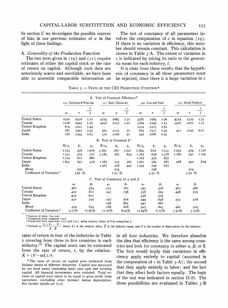
The test of constancy of all parameters in- volves the computation of c in equation (I9).
If there is no variation in efficiency, this num- ber should remain constant. This calculation is shown in Table 3-A. The extent of variation in c is indicated by taking its ratio to the geomet- ric mean for each industry, J.
It is clear from these results that the hypoth- esis of constancy in all three parameters must be rejected, since there is a large variation in c
in all four industries. We therefore abandon the idea that efficiency is the same among coun- tries and look for constancy in either a, /3, or S. The first would imply that variations in effi- ciency apply entirely to capital (assumed in the computation of c in Table 3-A); the second that they apply entirely to labor; and the last that they affect both factors equally. The logic of the test was indicated in section JI-D. The three possibilities are evaluated in Tables 3-B
TABLE 3. - TESTS OF THE CES PRODUCTION FUNCTION a
A. Test of Constant Efficiencyb
23I. Spinning & Weaving 31I. Basic Chemicals 34I. Iron and Steel 350. Metal Products
C c c c
w r c w r c w r c w r c
United States 2920 .0526 I.72 4754 .2083 2.3I 4387 *I984 2.96 43I4 *I359 2.35 Canada 2708 .0403 i.i6 4036 .2II5 2.0I 3769 *I740 2.13 3507 .I07I I.37 United Kingdom 874 .2022 I.44 .. I224 *I5I3 0.62
Japan 287 .I902 0.55 563 .2373 .70 664 .I9II 0.49 422 .2245 0.3I India 276 *I543 o.63 320 .2200 .5I 450 .2686 0.53
B. Test of Constant 5'
fi/a, at 'Yi fi/a, at 'Yi fi/ai at, 'i fi/a, aj 'Yi
United States I.I55 .536 i.oi6 3.283 .767 I.02I I.564 .6io I-733 I.039 .509 I-736 Canada I.352 .575 .77I 3.289 .767 .839 I.765 .638 I-378 i.i8o .541 I.292
United Kingdom I-5I4 .602 .880 .. I.. .265 .559 .857 Japan I.833 .647 .428 2.785 .734 .567 I.46I .584 .687 .968 .492 .6I9 India .. .. . 2.967 .748 .44I 1495 .599 .65 7
Mean .590 .754 .598 *5I4
Coefficient of Variationd 5.85 % 1.72 % 3.55 % 3.50 %
C. Test of Constancy of a and P at et at pis ai 6 i at ,8
United States .462 '534 .233 .765 .343 .536 .462 .480 Canada .452 .6iI .242 .796 .336 .593 .448 .529 United Kingdom 410 .62I .. .458 .579 ..
Japan .43 I .790 .297 .826 .444 .648 .53 5 .5I8 India .. .. .298 .883 .442 .66i
Mean .439 .639 .268 .8I8 .405 .603 .482 .509 Coefficient of Variationd 4.I7%o ii.85%o II.I9% 8.04% I2.84% 6.77% 77-4I% 3-79%
a Sources of data: See text. b Computed from equation (I9). c Computed from equations (2I) and (12), using country values of 3 in computing 'y. d Defined as - I X
_ where Xs is the country value, X is the industry mean, and N is the number of observations for the industry. NX
'3 The rates of return on capital were estimated from balance sheets of different industries. Capital was measured by net fixed assets (including land) plus cash and working capital. All financial investments were excluded. Total re- turns to capital were taken to be equal to gross profit from operations (excluding other income) minus depreciation. For further details see [I2].
236 THE REVIEW OF ECONOMICS AND STATISTICS
and 3-C by computing the coefficient of varia- tion for each parameter in each industry.
Of these three possibilities, the constancy of 8, implying neutral variations in efficiency, is much the closest approximation while there is little to choose between the other two. For the four industries taken together, the coefficient of variation in 8 is only 3.6 per cent, while it is more than twice as large for the other two pa- rameters. We therefore tentatively accept equa- tion (I2) or (I3) as the basic form of the CES production function. Constant c- and 8 charac- terize an industry in all countries, and differ- ences in efficiency are assumed to be concen- trated in y,.
The conclusion that observations on the same industry in different countries do not come from the same production function is so important that it should be tested in a way that does not depend on our particular choice of a production function. If in fact all countries fell on the same production function, homogeneous of degree one, then a high wage rate must arise from a high capital-labor ratio, which must, in turn, imply a low rate of return on capital. From Table 3 we see there is by and large an inverse correlation between wages and rates of return, but the variation in the latter seems much smaller than is consistent with the wide varia- tions in wage rates. This impression can be confirmed quantitatively with the aid of for- mula (7).
It is there noted that, for points on the same production function, homogeneous of degree one, the rate of return is a function of the wage rate, with an elasticity which is negative and equal in magnitude to the ratio of labor's share to capital's. We proceed as follows. Let v be the smallest observed value of this ratio. Then the elasticity of r, the rate of return, with re- spect to the wage rate, w, cannot exceed -v, so that,
og rli
where the subscripts refer to any two countries. If we choose the countries so that wo > w1, multiply through by the negative quantity log (w1/wo), and take antilogarithms, we find r1
',?) = ri, say. Then, if the two coun- tries were on the same production function, the rate of return in the low-wage country could not fall below the limit r1.
For each of the industries in Table 3, a com- parison was made of the rates of return in the lowest-wage country, with the corresponding lower bound r1, computed from the highest- wage country (the United States in each case). The results of this computation follow:
Industry 23I 3II 34I 350
r I.g9o .220 .269 .225
ii .244 .667 I.2I3 I.749
Thus in each case the actual rate of return in the lowest-wage country falls below the theo- retical minimum consistent with the assumption of a uniform production function, and in most cases very far below. The results of section A are thus strongly confirmed.
B. Effects of Varying Efficiency Since we have revised our interpretation of
the empirical evidence on the elasticity of sub- stitution, we can no longer take the regression coefficient b in section I as equal to o-. We now present a formula for determining o- from b when efficiency is known to vary with the wage rate and indicate the magnitude of the correc- tion involved. We then examine the residuals from the regression equations for further evi- dence of varying efficiency or other sources of bias in estimation.
i. Estimation of o-. It is plausible to assume that in each industry the efficiency parameter y varies among countries with the wage rate. Since the wage rate increases with both y and x, a country with high y is also likely to have been more efficient in the past and to have had high income and savings. Thus we expect x to be positively correlated with y across countries and y to increase with w. Assume for conven- ience that this variation takes the form:
(A ) (WA )e (29)
YB WB
where the subscripts refer to countries A and B. The effect of variation in efficiency on the out- put per unit of labor (y) can be shown from (25) to be:
YB YA WA
CAPITAL-LABOR SUBSTITUTION AND ECONOMIC EFFICIENCY 237
Substituting from (29) for the efficiency ratio and taking logs we get a formula comparable to equation (8) from which our elasticity esti- mates were derived:
log Y = (a + e - ea) log (W(3A Y'B WB
Comparing (8) and (3I), we see that the re- gression coefficient b is equal to (o-+e-eo-), or
b-e (32) b-e i - e
Therefore it is only when efficiency does not vary with w - i.e. when e = o - that b is equal to o-. For e > o, o- must be still smaller than b, and therefore, a fortiori, less than i
when b < i.
To get a rough idea of the magnitude of the correction, we normalized the y's in Table 3 sO that the United States value equals one in each case and then fitted log y to log w by least squares.14 We obtain the following result from the combined sample of I4 observations:
logy .323 log w -.039 R2 = .82. (.043)
The separate industries vary somewhat, but the number of observations in each is too small for reliable estimates. Another source of informa- tion on e is provided by the comparisons of Japan with the United States in section IV, which cover io manufacturing industries. Here the median value of (yJ/yu) is about .35, cor- responding to a value of e of about .5.
For values of b less than i, equation (32) shows that variation of efficiency with the wage rate will reduce the estimate of a-. Taking e= .3, values of b of .9, .8, and .7 yield values of .86, .7i, and .57. At the median value of b =.87 observed in Table 2, the corresponding C- is .8i.
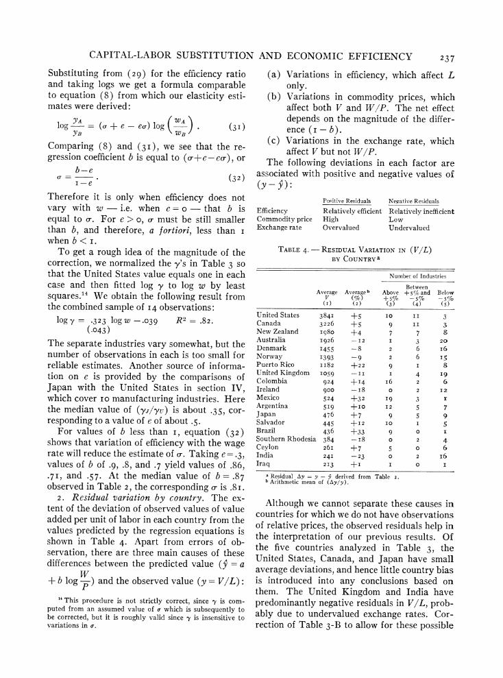
2. Residual variation by country. The ex- tent of the deviation of observed values of value added per unit of labor in each country from the values predicted by the regression equations is shown in Table 4. Apart from errors of ob- servation, there are three main causes of these differences between the predicted value (9 = a
+ b log p ) and the observed value (y = V/L):
(a) Variations in efficiency, which affect L only.
(b) Variations in commodity prices, which affect both V and W/P. The net effect depends on the magnitude of the differ- ence (i - b).
(c) Variations in the exchange rate, which affect V but not W/P.
The following deviations in each factor are associated with positive and negative values of (y - ):
Positive Residuals Negative Residuals
Efficiency Relatively efficient Relatively inefficient Commodity price High Low Exchange rate Overvalued Undervalued
TABLE 4.- RESIDUAL VARIATION IN (V/L) BY COUNTRY a
Number of Industries
Between Average Averageb Above +5% and Below
V (%) +5% -5% - 5s%io () (2) (3) (4) (5)
United States 384I +5 I0 II 3 Canada 3226 +5 9 II 3 New Zealand i980 +4 7 7 8 Australia I926 -I2 I 3 20
Denmark I455 -8 2 6 i6 Norway I393 -9 2 6 I5 Puerto Rico II82 +22 9 I 8 United Kingdom I059 -II I 4 I9
Colombia 924 +I4 i6 2 6 Ireland 900 -i8 0 2 I2
Mexico 524 +3 2 I9 3 X
Argentina 5I9 +I0 I2 5 7 Japan 476 +7 9 5 9 Salvador 445 + I2 Io I 5 Brazil 436 +33 9 0 1 Southern Rhodesia 384 -i8 0 2 4 Ceylon 26I +7 5 a 6 India 24I -23 0 2 i6 Iraq 2I3 +I I 0 I
a Residual Ay = y derived from Table 2. b Arithmetic mean of (Ay/y).
Although we cannot separate these causes in countries for which we do not have observations of relative prices, the observed residuals help in the interpretation of our previous results. Of the five countries analyzed in Table 3, the United States, Canada, and Japan have small average deviations, and hence little country bias is introduced into any conclusions based on them. The United Kingdom and India have predominantly negative residuals in V/L, prob- ably due to undervalued exchange rates. Cor- rection of Table 3-B to allow for these possible
"This procedure is not strictly correct, since y is com- puted from an assumed value of a which is subsequently to be corrected, but it is roughly valid since y is insensitive to variations in a.
238 THE REVIEW OF ECONOMICS AND STATISTICS
biases does not significantly affect the estimates of relative efficiency, however.
It seems plausible to interpret the systematic country deviations as due mainly to differences in exchange rates or in the level of protection. The United States, Canada, and Latin America have predominantly positive residuals, probab- ly due to overvalued exchange rates and (in Latin America) high levels of protection. West- ern Europe and India have predominantly negative deviations, probably because of rela- tively undervalued exchange rates. Variations in exchange rates and prices introduce a bias in estimation only if they are systematically related to the wage rate, which does not seem to be the case.
Although another comparative study [5] strongly suggests the importance of economies of scale, their effects are not apparent here in the residual variation in V/L. Larger plant size may account for part of the higher efficien- cy and positive deviations in the United States, but any such effect in other countries having large markets is concealed by the other sources of variation.
C. Effects of Price Variation Of the three sources of bias discussed in the
preceding section, the variation in commodity prices is probably the least important because it has a similar effect on both variables in the regression analysis. Since some data on rela- tive prices among countries are available, how- ever, it is desirable to test the magnitude of the error introduced by ignoring prices.
When commodity prices are known, the re- gression equation of (8) should be restated as follows, using the commodity price as the nu- meraire for both value added and wages:
log( a = + b log() (8a)
If prices are uncorrelated with wages, their omission affects the standard error but not the magnitude of the regression coefficient b. If prices are correlated with wages, the correction in the estimate of C- would be given by an equa- tion similar to (32 ).15 For example, an inverse relation between wages and prices would raise the estimate of C- for values of b less than i.
15If (PA/PB) = (WA/WB)t, then a = (b-f)/(i+f) if b is estimated from (8).
To test the quantitative significance of this correction, we have been able to assemble data for only two industries, neither of which cor- responds entirely either in coverage or time to the original data.'6 Estimating b alternatively from equations (8) and (8a) for the eleven countries available gives the following results:
Eq. (8) Eq. (8a)
Furniture (260) .8i4 .780
(.045) (.Io4) Knitting mill products (23 2) .692 .755
(.035) (.039)
In neither case is there a significant difference between the two estimates. Although this test by itself is by no means conclusive, such other evidence as is available on relative prices does not suggest that there are many sectors in which the estimate of o- would be significantly affected by this correction.
IV. Factor Substitution and the Economic Structure
Variations in production functions among in- dustries have a substantial effect on the struc- tural features of economies at different levels of income. In the present section, we shall in- vestigate the effects on factor proportions, com- modity prices, and comparative advantage that stem from differences in the parameters of the CES production function.
16 The sectors covered are both consumer goods, since we were unable to find comparable data on intermediate prod- ucts for any substantial number of countries. The prices used for sector 232 apply to all clothing rather than to 232
only. The price indexes are as follows for the ii countries: Price of Furniture Price of Knitted Goods
United States I00.00 100.00
Canada 154-70 148.9I
Australia 8I.95 73-58 New Zealand 94.82 I03.46 United Kingdom 66.46 60.30 Denmark 89.4I 77-I3
Norway 94.3 7 89.90 Argentina 223.00 139.0I Brazil 145.90 97.20 Colombia I82.60 2 25.70
Mexico I75.80 I24-58
Data are taken from Internationaler Vergleich der Preis fir die Lebenshaltung, Ergainzungsheft Nr. 4 Zu Reiche 9, Einzelhandelspreise in Ausland, Verlag W. Kohlhammer GMBH, Stuttgart und Mainz, Jahrgang, I959. The original data are in deutschmark purchasing power equivalents, from which the implied prices indexes were derived by taking the United States as a base. The exchange rates used in convert- ing the prices to dollars were the ones that were used in section I.
CAPITAL-LABOR SUBSTITUTION AND ECONOMIC EFFICIENCY 239
To carry out this analysis, it is necessary to have some indication of the values of the three parameters in sectors of the economy other than those examined in section I, and hence to have some direct observations on the use of capital. For this purpose, we shall determine the pa- rameters in the production function from data on comparable sectors in Japan and the United States. Although these two-point estimates may have substantial errors in individual sectors, the over-all results of this second method of estimation support the principal results of our earlier analysis and lead to some more general conclusions.
A. Production Functions from US..-Japanese Comparisons
The United States and Japan were selected for this analysis because of the availability of data on factor use, factor prices, and commodi- ty prices in a large number of sectors.'7 They also are convenient in having large differences in relative factor prices and factor proportions. The errors involved in estimating the elasticity of substitution are therefore less than they would be if there were less variation in the ob- served values. (For the data in section I, esti- mates based only on the United States and Japan differed by less than i O per cent on the average from the regression estimates.)
The elasticity of substitution can be esti- mated from these data by means of equation (24):
Xi (K/L) j rj XU (K/L) u Wu
ru J
where subscripts indicate the country. This method of estimation has the advantage of uti- lizing direct observations of capital as well as labor and of being independent of the varying value of the efficiency parameter y.
The data for this calculation are taken from input-output studies in the two countries and are summarized in Table 5. The main concep-
tual difference from section III is in the defini- tion of capital, which here includes only fixed capital. The labor cost in Japan makes allow- ance for the varying proportions of unpaid family workers in each sector. The variation in relative factor costs shown in column (4) is due entirely to differences in labor costs, since the relative cost of capital is assumed to be the same for all sectors.
The values of C- derived by this method vary considerably more than those derived from wage and labor inputs alone in section I. How- ever, for the I2 manufacturing sectors in which both are available, there is a significant correla- tion of .55 between the two estimates.'8 The weighted median of a- for these sectors is .93 as compared with .87 by the earlier analysis. The median c- is also .93 for all manufacturing. The omission of working capital provides a plau- sible explanation of this difference, since the little evidence available indicates that stocks of materials and goods in process are generally as high in low-wage as in high-wage countries. The elasticity of substitution between working capital and labor is therefore probably much less than unity. This correction is particularly important in trade and in manufacturing sectors having small amounts of fixed capital.
Since these two-country estimates are rea- sonably consistent with our earlier findings for the manufacturing sectors, we will tentatively accept them as indicative of elasticities of sub- stitution in non-manufacturing sectors, with qualifications for the omission of working capi- tal. Here the most notable results are the rela- tively high elasticities in agriculture and min- ing, and the low elasticity in electric power.'9 In trade, the omission of working capital prob- ably leads to a serious overestimate of the elas- ticity of substitution, while for other services we have no comparable data. The evidence of relative prices, however, suggests an elasticity for personal services, at least, of substantially less than unity.
"7The compilation of these data on a comparable basis has been done by Gary Bickel, who is conducting an exten- sive analysis of the relation between factor proportions and relative prices in the two countries. Further discussion of the data is given by Bickel [41.
18 In some sectors the correspondence between the in- dustries covered is very imperfect because the earlier esti- mates are on a 3-digit basis and cover only part of the 2-
digit class. 19 The transport sector involves a very large difference
in product mix, and the reliability of the estimate is doubtful.

240 THE REVIEW OF ECONOMICS AND STATISTICS
CHART I.-C.E.S. PRODUCTIONS FUNCTIONS
L LABOR
x-JAPANESE FACTOR PROPORTIONS
\D LU.S. FACTOR PROPORTIONS
\ / | PARAMETERS
/ ~~ ~~~~~~~~~~~A 1 5 .25
/ E C .8 .2
A / - x=2.0 D .8 .8
A ~~~~~~~~ / ~~~~~~E .4 .05
C
x~~~-
A=S~~~~~~~~~~~~~~ - ~~~~~~~~~~D CAPITAL
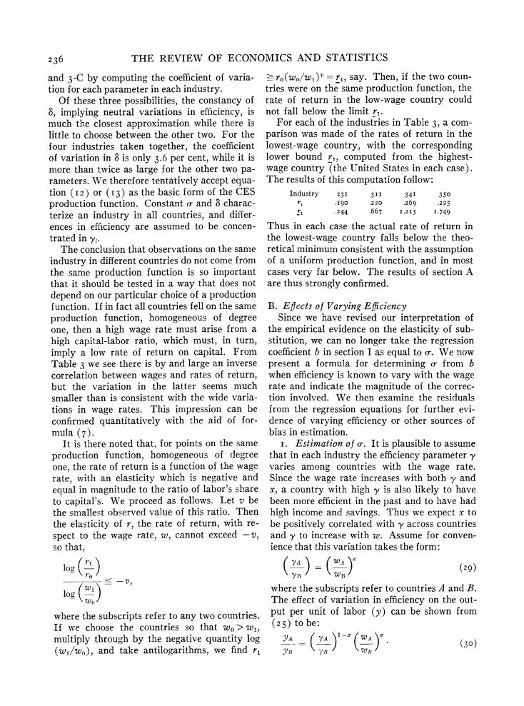
On the basis of this comparison, we have con- structed the five isoquants in Chart i to illus- trate the range of variation in o- and 8. Sectors
in Table 5 corresponding approximately to these sets of values are indicated in Table 6. The
TABLE 6.- ILLUSTRATIVE COMBINATIONS OF cy AND 8
6 Examples
A I.I5 .25 Agriculture, mining, paper, non-ferrous metals B i.O .2 Steel, rubber, transport equipment C .8 .2 Textiles, wood products, grain millling D .8 .8 Electric power E .4 .05 Apparel, personal services
effect of increasing o- in flattening the isoquant is shown by comparing E, C, B and A, while the effect of 8 on the capital intensity is shown by comparing C and D. The optimum factor proportions at average Japanese and United States factor prices are also indicated to illus- trate the discussion in the next section.
TABLE 5.- CALCULATION OF ELASTICITY OF SUBSTITUTION FROM FACTOR INPUTS AND FACTOR PRICES: JAPAN VS. UNITED STATESa
Capital Intensity Parameters Estimated Regression - Relative Factor Cost Estimate No. Sector Xu XJ XJ/Xu (Wj/Wu X ru/rj) a0 of a
(I) (2) (3) (4) (5) (6) (7)
I Primary Production
OI, 02, 03 Agriculture I9.5I .367 .019 .036 I.20 .396 04 Fishing 3.24 .490 .J52 *I33 .94 .20I Io Coal mining 4.87 .534 .IIO .093 .93 .i82
I2 Metal mining I3.34 .566 .042 J107 I.4I .2I5
I3 Petroleum & natural gas 40.57 .722 .oi8 .o96 I.7I .265
I4, I9 Non-metallic minerals IO-37 .777 .075 .III i.i8 .260
II Manufacturing
205 Grain mill. production 5.36 .549 .J03 .o6o .8i .286 .9I 20, 22 Processed food 5-II .374 .073 .o6I .93 .327 .82 23 Textiles 2.76 .340 .J23 .073 .80 .J59 .8I
232, 243 Apparel .99 .329 .332 .07I .42 .055
241, 242, 29 Leather products I.0I J.90 .I89 .o98 .72 .05I .86
25, 26 Lumber and wood prod. 3.58 .3I0 .o87 .054 .84 .i98 .87 27 Paper 7.3I .528 .072 .099 I.I4 .204 .96 28 Printing and publishing 3.45 .I43 .042 .072 I.2I .092 .87 30 Rubber 3.73 .332 .o89 .o84 .98 .I47
3I Chemicals 8.32 I.I25 .I35 *I57 .90 .325 .85 321, 329 Petroleum products 38.I8 .360 .094 .J5I I.04 .550
322,329 Coal 35.85 I.895 053 .I I3 I.35 .365 33 Non-metal. min. prod. 5.95 *4I4 .070 .o84 I.08 .J97 .95 34I, 35 Iron and steel 8.6o .986 .JI5 .II5 I.00 .273 .85 342 Non-ferrous metals II.45 I.I5I .JOI .I23 I.I0 1.287 I.0I 36, 37 Machinery 4.86 .469 .o97 .o83 .93 .i87 .87 38I Shipbuilding 4.76 .477 .IOO .094 .97 I 74
382 Transport equipment 5.oI .378 .075 .o83 I.04 .j69
III Utilities and Services
5II Electric power 46.I3 IO.50 .228 .I64 .82 .8I9
6i Trade 5.93 .349 .o59 .079 I.I2 .I87 7I Transport I5.7I .3I6 .020 .io6 I.74 .I70
a SOURCES: COlS. (I), (2), and (4) are taken from Bickel [4], based on U.S. and Japanese input-output materials; rjlru assumed to be 1.47 for all sectors. Col. (5) is calculated from equation (33). Col. (6) is calculated from equation (2oa). Col. (7) aggregated from Table 2 using the average proportions of value added in the two countries as weights.
CAPITAL-LABOR SUBSTITUTION AND ECONOMIC EFFICIENCY 24I
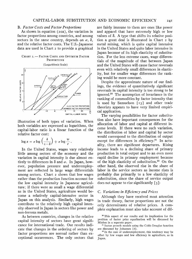
B. Factor Costs and Factor Proportions As shown in equation (2oa), the variation in
factor proportions among countries, and among sectors in the same country, depends on o-, 8, and the relative factor costs. The U.S.-Japanese data are used in Chart 2 to provide a graphical
CHART 2. - FACTOR COSTS AND OPTIMUM FAC TOR PROPORTIONS
(Logarithmic Scale)
20 -CHEMICALS L
TEXTILES
u10 0ON APPAREL METAL FERR
MININ METAL
w 1 < C / gPOWER
AGIULTURE
2 - X
/-U.S. FACTOR PROPORTIONS
-JAPNESE FACTOR PROPORTIONS
I .0 2 5 10 20 K
CAPITAL-LABOR RATIO
illustration of both types of variation. When both variables are expressed as logarithms, the capital-labor ratio is a linear function of the relative factor cost:
log x = a log + w log-.
In the United States, wages vary relatively little among sectors of the economy and the variation in capital intensity is due almost en- tirely to differences in 8 and o-. In Japan, how- ever, population pressure and underemploy- ment are reflected in large wage differentials among sectors. Chart 2 shows that low wages rather than the production function account for the low capital intensity in Japanese agricul- ture; if there were as small a wage differential as in the United States, agriculture would be- come a relatively capital-intensive sector in Japan on this analysis. Similarly, high wages contribute to the relatively high capital inten- sity observed in Japan in sectors like power and non-ferrous metals.
As between countries, changes in the relative capital intensity of sectors have great signifi- cance for international trade. Our results indi- cate that changes in the ordering of sectors by factor proportions are normal rather than ex- ceptional occurrences. The only sectors that
are fairly immune to them are ones like power and apparel that have extremely high or low values of 8. A type that shifts its relative posi- tion a great deal is illustrated in Chart 2 by metal mining, which is quite capital intensive in the United States and quite labor intensive in Japan because of its high elasticity of substitu- tion. For the less extreme cases, wage differen- tials of the magnitude of that between Japan and the United States will cause factor reversals even with relatively small differences in elastic- ity, but for smaller wage differences the rank- ing would be more constant.
Despite the approximate nature of our find- ings, the evidence of quantitatively significant reversals in capital intensity is too strong to be ignored.20 The assumption of invariance in the ranking of commodities by factor intensity that is used by Samuelson [ I 3 ] and other trade theorists appears to have very limited empiri- cal application.
The varying possibilities for factor substitu- tion also have important consequences for the allocation of labor and capital at different in- come levels. If there were no such variation, the distribution of labor and capital by sector would correspond to the distribution of output except for differences in efficiency.2' In actu- ality, there are significant departures. Rising income leads to a declining share of primary production in total output and to an even more rapid decline in primary employment because of the high elasticity of substitution.22 On the other hand, the observed rise in the share of labor in the service sectors as income rises is probably due primarily to a low elasticity of substitution, since the share of service output does not appear to rise significantly [ 5]
C. Variations in Efficiency and Prices Although they have received most attention
in trade theory, factor proportions are not the only determinants of relative prices. A com- plete explanation must also take account of dif-
'This aspect of our results and its implication for the problem of factor price equalization will be discussed by Minhas in a separate paper.
21 Sector growth models using the Cobb-Douglas function are discussed by Johansen [8].
22 In the case of underemployment, this tendency may be offset by low wages and low efficiency in agriculture, as in Japan.
242 THE REVIEW OF ECONOMICS AND STATISTICS
ferences in relative efficiency among countries and industries, about which there is little sys- tematic knowledge. We first present measures of relative efficiency in each sector derived from the Japan-United States comparison and then explore the combined effects of variation in all three parameters on relative prices among countries.
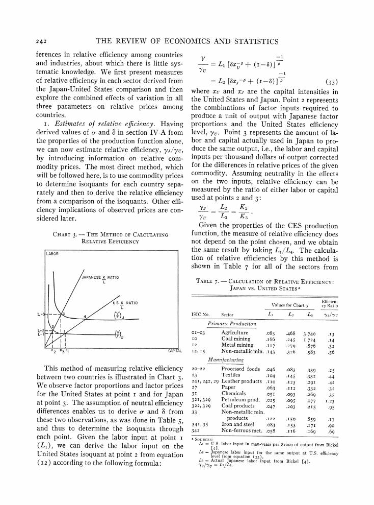
i. Estimates of relative efficiency. Having derived values of o- and 8 in section IV-A from the properties of the production function alone, we can now estimate relative efficiency, yJ/yu, by introducing information on relative com- modity prices. The most direct method, which will be followed here, is to use commodity prices to determine isoquants for each country sepa- rately and then to derive the relative efficiency from a comparison of the isoquants. Other effi- ciency implications of observed prices are con- sidered later.
CHART 3. - THE METHOD OF CALCULATING RELATIVE EFFICIENCY
LABOR
JAPANESE K RATIO
U K RATIO L
L- -2- L-2 I
K2 K3 K1 CAPITAL
This method of measuring relative efficiency between two countries is illustrated in Chart 3. We observe factor proportions and factor prices for the United States at point i and for Japan at point 3. The assumption of neutral efficiency differences enables us to derive o- and 8 from these two observations, as was done in Table 5, and thus to determine the isoquants through each point. Given the labor input at point i (L,), we can derive the labor input on the United States isoquant at point 2 from equation (I2) according to the following formula:
v -1 - L1 [8x P + (I P
Yu -1
- L2 [8Xj-P + (I -8) ] P (33) where xu and XJ are the capital intensities in the United States and Japan. Point 2 represents the combinations of factor inputs required to produce a unit of output with Japanese factor proportions and the United States efficiency level, yu. Point 3 represents the amount of la- bor and capital actually used in Japan to pro- duce the same output, i.e., the labor and capital inputs per thousand dollars of output corrected for the differences in relative prices of the given commodity. Assuming neutrality in the effects on the two inputs, relative efficiency can be measured by the ratio of either labor or capital used at points 2 and 3:
Y.T L2 K2
Yu L3 K3 Given the properties of the CES production
function, the measure of relative efficiency does not depend on the point chosen, and we obtain the same result by taking L1jL4. The calcula- tion of relative efficiencies by this method is shown in Table 7 for all of the sectors from
TABLE 7. - CALCULATION OF RELATIVE EFFICIENCY: JAPAN VS. UNITED STATESa
Efficien- Values for Chart 3 cy Ratio
ISIC No. Sector LI L. L3 J/lyu
Primiary Production
OI-03 Agriculture .083 *468 3.740 .J3 IO Coal mining .I66 .245 1.724 .I4 12 Metal mining .II7 .2 79 .876 .3 2 14, I5 Non-metallicmin. J143 .326 .583 .56
Manufcturing
20-22 Processed foods .046 .083 .339 .25
23 Textiles .104 .I45 .332 .44 24I, 242, 29 Leather products .IIO .123 .291 .42
27 Paper .o63 .112 .33 2 .3 2 3I Chemicals .05I .093 .269 .35 321, 329 Petroleum prod. .025 .095 .077 1.23
322, 329 Coal products .047 .203 .2I5 .95 33 Non-metallic min.
products .122 .150 .859 .17
341, 35 Iron and steel .o83 .153 .17I .90
342 Non-ferrous met. .058 .II6 .I69 .69 a SOURCES:
Li = U.S. labor input in man-years per $IOOO of output from Bickel L4W.
L2= Japanese labor input for the same output at U.S. efficiency level from equation (33).
L3 = Actual Japanese labor input from Bickel [41. yJl/8u = L2/L3.
CAPITAL-LABOR SUBSTITUTION AND ECONOMIC EFFICIENCY 2 43
Table 5 for which relative commodity prices are also available.
In manufacturing, the median efficiency level is .43 (or .35 weighted by value added) which is about the same as the average ratio of Japanese and American efficiency determined in section III.23 In primary production it is considerably lower, with agriculture and coal mining only one seventh of the American level.
Three factors may be suggested to explain these differences in relative efficiency.
(i) Limited natural resources doubtless ex- plain a large part of the lower efficiency of capi- tal and labor in primary production in Japan.
(ii) Competitive pressure in exports and import substitutes was suggested in [6] to be a cause of more rapid productivity increases in these sectors in Japan. Inefficient sectors (agri- culture, mining, food, non-metallic mineral products) produce for the home market in Japan and are protected by either transport costs or tariffs from foreign competition.
(iii) Relatively efficient sectors in Japan (petroleum products, coal products, steel, non- ferrous metals) are characterized by high capi- tal intensity, large plants, and continuous proc- essing. There may be technological reasons why it is easier to achieve comparable efficiency lev- els under these conditions.
Tests of these and other hypotheses regard- ing relative efficiency must await similar studies for other countries.
2. Relative commodity prices. Since we now have estimates of all three parameters in the production function, we can investigate their im- portance to the determination of relative com- modity prices.
To do this, we substitute representative val- ues of wlr 24 for the United States, Western Europe, and Japan in formula (28):
| __ (__) A 1_
P B W-8 YA ( A(WB A -
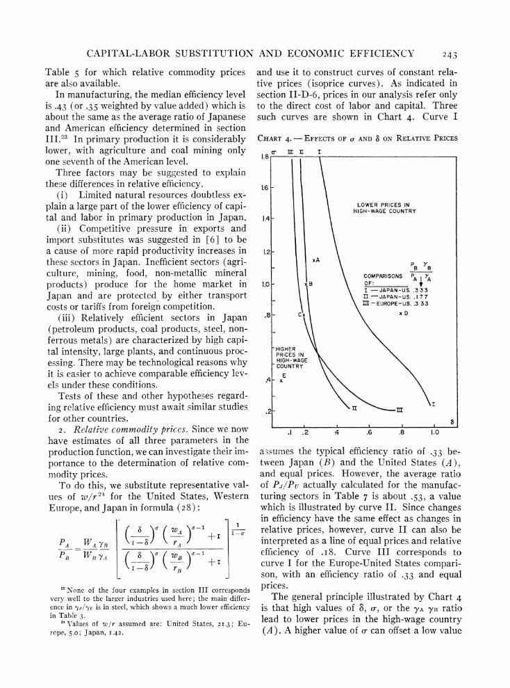
and use it to construct curves of constant rela- tive prices (isoprice curves). As indicated in section II-D-6, prices in our analysis refer only to the direct cost of labor and capital. Three such curves are shown in Chart 4. Curve I
CHART 4. - EFFECTS OF C AND 8 ON RELATIVE PRICES
CIllrIE I
1.8
1.6
LOWER PRICES IN HIGH-WAGE COUNTRY
14 -
1.2- xA
pB rB COMPARISONS P tA
1.0 x B OF: A4 I -JAPAN-U.S. .333
\II-JAPAN-US. .17 7 M II\EUROPE-US. .3 33
.8 C ;x xD
HIGHER PRICES IN HIGH-WAGE COUNTRY
.2-
.1 .2 4 .6 .8 1.0
assumes the typical efficiency ratio of .33 be- tween Japan (B) and the United States (A), and equal prices. However, the average ratio of Pj/Pu actually calculated for the manufac- turing sectors in Table 7 is about .53, a value which is illustrated by curve II. Since changes in efficiency have the same effect as changes in relative prices, however, curve II can also be interpreted as a line of equal prices and relative efficiency of .i8. Curve III corresponds to curve I for the Europe-United States compari- son, with an efficiency ratio of .33 and equal prices.
The general principle illustrated by Chart 4 is that high values of 8, a-, or the YA 71B ratio lead to lower prices in the high-wage country (A). A higher value of o- can offset a low value
23 None of the four examples in section III corresponds very well to the larger industries used here; the main differ- ence in yJ/yu is in steel, which shows a much lower efficiency in Table 3.
24 Values of w/r assumed are: United States, 2I.3; Eu- rope, 5.o; Japan, I.42.
244 THE REVIEW OF ECONOMICS AND STATISTICS
of 8 to a considerable extent. Representative combinations of o- and 8 are also shown in Chart 4, where the five illustrative sets of production parameters of Chart i are plotted. For a con- siderable number of the industrial sectors in Table 5, illustrated by the range of points A-B-C, variation in the elasticity of substitu- tion seems to be more important than variation in 8 in determining relative prices.
Actual price differences between Japan and the United States are affected as much by the cost of purchased inputs as by the value added component. Calculations for the ten manufac- turing sectors in Table 7 based on (28) give a range of direct costs in Japan of .3 to .95 of the United States value, but this element is only about 35 per cent of total cost on the average. The average price of purchased inputs in these sectors ranges from .93 to I.70 of their cost in the United States, which more than makes up for the lower cost of the factors used directly.25 An adequate explanation of the differences in relative prices therefore requires an analysis of total factor use rather than of the direct use by itself.26
V. Substitution and Technological Change A. Technological Change, Labor's Share,
and the Wage Rate i. Historical changes in labor's share. In
section II-D-5, some implications of the CES production function for time series were de- rived. In particular (25), it was shown that labor's share was governed by the relation,
=L (-) . (25a) V 7Y
Under the assumption of neutral technological change, the only parameter that varies is y. For an elasticity of substitution less than one,
labor's share rises when wage rates increase more rapidly than technological progress. (For o > I the relation is reversed; for o- = I, we are in the familiar Cobb-Douglas case where labor's share is independent of both neutral techno- logical progress and wage-rate changes.) The historically observed relative constancy of la- bor's share can be understood in these terms; labor's share is the resultant of offsetting trends; and further, for o- not too far from I, it is a relatively insensitive function of them.27
If in particular we add the assumption that technological change proceeds at a constant geometric rate, we have [cf. (26)]
wL log - = ao + a, log w + a2 t, (34)
where ao = crlog (I-8) + ( I-I) logyO, (35) a, = I-,a2 = -(I-). (35a)
From estimates of a, and a2, it is easy, from (35a), to solve for estimates of X and of the elasticity of substitution, which is I-a,. Equation (34) was fitted by least squares to the data for the United States non-farm production, I909-49, given in Solow; 28 it was found that a,= .43I and a2 =- .003. The corresponding estimate of o- is .569 and that of X = .oo8, which corresponds to an annual rate of growth of pro- ductivity of i.83 per cent. This figure agrees pretty well with most earlier estimates (Solow, [I4], 36, gives i.5 per cent; see also Abramo- vitz [ I ], I I).-
We can test for the significance of the differ- ence of the elasticity of substitution from its Cobb-Douglas hypothetical value of I, which implies that a, and a2 are both zero. The test then is equivalent to that for the significance of the multiple correlation coefficient, which has a value of .740; an F-test shows that, for 4I
25 Japan is somewhat exceptional among industrial coun- tries in its dependence on imported materials, and between another pair of countries the variation in direct factor cost might be more indicative of the variation in total cost of production.
' The extent to which price differences between the two countries can be explained by total factor use is analyzed by Bickel [4]. He shows that the average capital intensity (reflecting 3) combined with the ratio of total factor inten- sities, which indicates a weighted average elasticity of sub- stitution throughout the economy, gives a reasonably good prediction of relative prices. This result can be derived from equation (28) on the assumption that yJ/yu does not vary greatly.
27 However, (25a) does not provide a true causal analysis of the changes in labor's share if the wage rate is deter- mined simultaneously with the other variables of the sys- tem. The wage rate may be treated as exogenous as in, for example, Lewis's model of economic growth [ii], which is applicable to those economies in which there is large rural disguised unemployment.
28 The data were derived from the columns of Table i in Solow [I4] as follows: wL/V is obtained by subtract- ing column (4) (share of property in income) from i; w = (wL/V) (V/L), where V/L is column (5) (private non- farm GNP per man-hour); t is time measured in years from I929.
CAPITAL-LABOR SUBSTITUTION AND ECONOMIC EFFICIENCY 245
observations, the value is highly significant. The alternative of capital-output and labor- output ratios which are fixed at any instant of time corresponds to a, = i. Since the standard error of estimate of a, is .042, this hypothesis must also be rejected.
As in the cross-section studies, there is strong evidence that the elasticity of substitution is between zero and one. There may be some in- consistency with the results of the cross-section study of manufacturing sectors in section I in that the time series estimate of the elasticity of substitution is considerably lower than that found in the international comparisons. How- ever, the time series data include services about whose elasticity of substitution we know little.
Estimation of (34) by least squares must be regarded only as an approximation. There is an unknown simultaneous equations bias in the procedure. However, more accurate methods would require a more detailed specification of the types of errors appearing in the marginal productivity relation (34) and the production function, a specification that we are not pre- pared to make. The results must therefore be regarded as tentative; the difficulties noted in section B below are undoubtedly related to the choice of estimation methods.
2. A test of the production function. As in the cross-section study, we can try to test the production function implied by the preceding results; this test, again, is a stringent one in that it uses capital data which have not been employed in fitting the marginal productivity relation. The fitting of (34) has yielded esti- mates of o- and X but only one relation (35) between y0 and 8. We now use capital data to obtain separate estimates of these parameters. Define,
I q=
antilog (?
from (35), since
P= (I-cr)
p
o
(I-8c)
If we let y = yo (io)t in the production func-
tion and express yo in terms of q, we find, after some manipulation that,
X- = -8 ) (36)
where,
XI = q (K )IPxt x2 K= (K) (36a)
As in the analysis of the international compari- sons, the strictest test would be the constancy of the left-hand side of (36), which would im- ply an exact fit and simultaneously give an esti- mate of 8. In the absence of strict constancy, we can estimate 8/( i-8) as the average, X- X2; this yields the estimate, 8= .5I9.29
If we measure time in years from I929, the value of ao was -.o8o, so that the value of yo is .584. The production function for United States, non-farm output, I929-49, is given by,
V = .584 (IOI83)t (.5I9 K- .756
+ .48i L- .756)-1-322 (37) We have tested this production function
against actual output; the fit appears satisfac- tory. Out of 4I years, the prediction error is not more than 4 per cent of the predicted value in 22 years and not more than 8 per cent in 3I.
The maximum errors in prediction were - I3.3
per cent (I933) and +IO.7 per cent (I909).
It is further significant that all five of the years in which actual output fell short of pre- dicted by more than 8 per cent were the depres- sion years, I930-34. This is reasonable on theoretical grounds; the immobility created by severe unemployment of both capital and labor causes inefficiency in the utilization of those resources that are employed (for a develop- ment of this argument, see Arrow [31 ). If the depression years had been excluded we might have expected a still better fit.
B. Relative Shares and the Capital-Labor Ratio
Another test, with less satisfactory results, is that given by (23). In logarithmic form, the ratio of labor's to capital's share is related to the capital-labor ratio by:
9 X1 and X2 are again calculated from Table i in [I4]; K/L is given in column (6) (employed capital per man- hour); K/V = (K/L) (VIL), where V/L is column 5.
246 THE REVIEW OF ECONOMICS AND STATISTICS
log( W ) = log(I-8) log (38)
For p positive, the steady secular rise in the capital-labor ratio would give rise to an increase in labor's share, but one which would be very moderate unless p were large.
Relation (38) was fitted by least squares; the data were the same as those used in the preced- ing section.30 The estimate of p was - .095, which implies an elasticity of substitution slight- ly greater than i. The standard error of esti- mate of p is .o98, so that the hypothesis of a positive value for p is not rejected, but the values are inconsistent with those found in sec- tion A.
The reasons for the contradiction of the two estimates are not clear. If (34) and the produc- tion function (37) both held exactly, then (38) would have to hold exactly with the same values of p and 8. Hence the discrepancy must be due to the different assumptions about the errors implicit in the statistical estimation methods. This problem remains an open one for the present.
Kravis ( [9], 940-4 ) has applied essentially the same method, in the form of (24), to data for the entire economy (rather than only the non-farm portions, as here). His estimate of the elasticity of substitution is .64, which is much closer to the results of section A.
VI. Conclusion
This article has touched on a wide range of subjects: the pure theory of production, the functional distribution of income, technological progress, international differences in efficiency, the sources of comparative advantage. In part this broad scope reflects, as our introduction suggests, the fundamental economic significance of the degree of substitutability of capital and labor. In part it points to a wide variety of unsettled questions which are left for future research and better data. (In part, no doubt, it is simply due to the large number of authors of the paper! ) Since our work does not lend itself to detailed summary, we content ourselves with a brief reprise of some of our findings, some speculation about others, and some suggestions for future research.
30 wL/rK = (wL/V)/[i - (wL/V)].
A. Findings We have produced some evidence that the
elasticity of substitution between capital and labor in manufacturing may typically be less than unity. There are weaker indications that in primary production this conclusion is re- versed. Although our original evidence comes from an analysis of the relationship between wages and value added per unit of labor, we have interpreted it by introducing a new class of production functions, more flexible and (we think) more realistic than the standard ones.
Although we began our empirical work on the naive hypothesis that observations within a given industry but for different countries at about the same time can be taken as coming from a com- mon production function, we find subsequently that this hypothesis cannot be maintained. But we get reasonably good results when we replace it by the weaker, but still meaningful, assump- tion that international differences in efficiency are approximately neutral in their incidence on capital and labor. A closer analysis of inter- national differences in efficiency leads us to suggest that this factor may have much to do with the pattern of comparative advantage in international trade.
Finally, our formulation contributes some- thing to the much-discussed question of func- tional shares. If, on the average, elasticities of substitution are less than unity, the share of the rapidly-growing factor, capital, in national product should fall. This is what has actually occurred. But in the CES production function it is possible that increases in real wages be off- set by neutral technological progress in their effect on relative shares.
B. Speculation In his original work on what has since come
to be known as the "Leontief scarce-factor par- adox," Professor Leontief [iO] advanced tenta- tively the hypothesis that the United States exports relatively labor-intensive goods not be- cause labor is relatively abundant when meas- ured conventionally, but because the efficiency of American labor is something like three times the efficiency of overseas labor. In our notation, this amounts to the suggestion that interna- tional differences in efficiency take the form of variations in 8/a or, equivalently, of 8. We
CAPITAL-LABOR SUBSTITUTION AND ECONOMIC EFFICIENCY 247
have proposed instead the hypothesis that //a is constant across countries, while differences in efficiency are neutral. But we have also found some slight indications, in comparing Japan and the United States, that the American advantage in efficiency tends to be least in capital-intensive industries. This pattern, if it were verified, would seem to lead to an alternative interpreta- tion of the Leontief phenomenon. But it also opens wide the question of why this association between differential efficiency and capital in- tensity should occur. Some possible explana- tions were mentioned in section IV-C, but the reader can think of others. We may be missing something important by excluding third factors, or external effects, or the importance of gross investment itself as a carrier of advanced tech- nology into a sector.
Another active area of economic research where our results may have some interest is the theory of economic growth. An as yet unpub- lished paper 31 by J. D. Pitchford of Melbourne University considers the introduction of a CES production function into a macroeconomic mod- el of economic growth and concludes that at least in some cases this amendment restores to the saving rate some influence on the ultimate rate of growth. Even more interesting are the possible implications for disaggregated general equilibrium models. Given systematic inter- sectoral differences in the elasticity of substitu- tion and in income elasticities of demand, the possibility arises that the process of economic development itself might shift the over-all elas- ticity of substitution.
C. Unsettled Questions Our general reference under this heading is
passim. To begin with, as usable capital data for more countries and more industries become available, all of our results become subject to check for validity and generality. In particu- lar, our speculations about the causes of vary- ing efficiency are based primarily on compari- sons between Japan and the United States. A more extensive study might easily controvert them.
Another loose end has to do with the question
of returns to scale. We note that the stringent test for constant returns to scale and constancy of all parameters clearly has to be rejected. But it would be useful to explore the possibility of increasing returns to scale on a broader front. In view of equation (I6) is there some choice of the function C(K) which would yield a test on increasing returns? What light might this throw on the international comparisons, espe- cially in connection with the less developed economies?
Finally, the whole question of further dis- aggregation calls out for exploration. We have in mind here not so much a finer industrial breakdown as a finer input breakdown. Can our labor and capital inputs be usefully sub- divided? How about natural resource and pur- chased material inputs?
"1Now published: "Growth and the Elasticity of Factor Substitution," Economic Record, December I960, 49I-500. (Note added in proof.)
References
i. M. Abramovitz, "Resource and Output Trends in the United States Since I870," American Econom- ic Review, XLVI (May I956), 5-23.
2. R. G. D. Allen, Mathematical Analysis for Econo- mists (London, I938).
3. K. J. Arrow, "Toward a Theory of Price Adjust- ment," in M. Abramovitz et al., The Allocation of Economic Resources (Stanford, California, I959),
4I-5I. 4. G. W. Bickel, "Factor Proportions and Relative
Prices in Japan and the United States," paper read to the summer meeting of Econometric Society (Stanford, California, August 1960).
5. H. B. Chenery, "Patterns of Industrial Growth," American Economic Review, L (September I960), 624-54.
6. H. B. Chenery, S. Shishido, and T. Watanabe, "The Pattern of Japanese Growth, I9I4-54," June 1960
(mimeog.) 7. G. H. Hardy, J. E. Littlewood, and G. P6lya, In-
equalities (Cambridge, England, I934).
8. L. Johansen, "Rules of Thumb for the Expansion of Industries in a Process of Economic Growth," Econometrica, xxviii (I960), 258-7I.
9. I. B. Kravis, "Relative Income Shares in Fact and Theory," American Economic Review, XLIX (I959), 9 I 7-49.
Io. W. W. Leontief, "Domestic Production and For- egn Trade: The American Capital Position Re- examined," Proceedings of the American Philo- sophical Society. 97 (953), 33 I-49.
i i. W. A. Lewis, "Economic Development with Un- limited Supplies of Labor," The Manchester School, XXII (1954), I39-9I.
I 2. B. S. Minhas, "An International Comparison of the Rates of Return on Capital in Manufacturing
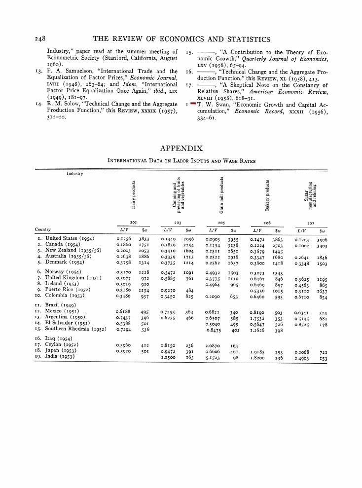
248 THE REVIEW OF ECONOMICS AND STATISTICS
Industry," paper read at the summer meeting of Econometric Society (Stanford, California, August 1960).
I 3. P. A. Samuelson, "International Trade and the Equalization of Factor Prices," Economic Journal, LVIII (I948), I63-84; and Idem, "International Factor Price Equalization Once Again," ibid., LIX
( I949 ), I 8I-97 - I4. R. M. Solow, "Technical Change and the Aggregate
Production Function," this REVIEW, XXXIX (I957), 3I 2-20.
I 5. , "A Contribution to the Theory of Eco- nomic Growth," Quarterly Journal of Economics, LXV (1956), 65-94.
I6. , "Technical Change and the Aggregate Pro- duction Function," this REVIEW, XL (I958), 4I3.
I 7. " "A Skeptical Note on the Constancy of Relative Shares," American Economic Review, XLVIII (1958), 6I8-3I.
I8. T. W. Swan, "Economic Growth and Capital Ac- cumulation," Economic Record, XXXII (1956),
334-6I.
APPENDIX
INTERNATIONAL DATA ON LABOR INPUTS AND WAGE RATES
Industry
bo ~~~~~~~~~~~~~~~~~~~~~~~~bO cn cn
; CD~~~~~~~~~~~~~b
202 203 205 206 207
Country L/V $CL L/V $cL L/V $cL LIV $co L/V $L
i. United States (Ig54) O.I256 3833 0.I449 2956 0.0903 3955 0-I472 3863 O.I203 3906 2. Canada (I954) o.i860 2751 O.I859 2254 O.I254 3I38 0.2224 2503 O.I002 3403 3. New Zealand (I955/56) 0.2003 2053 0.34IO i604 0.23II I85I 0.3679 I495 4. Australia (I955/56) 0.2638 i886 0.3339 1715 0.2522 I9I6 0.3347 i68o 0.264I I846 5. Denmark (I954) 0.3758 I3I4 0.3735 I2I4 0.2562 I657 0.3600 I4I8 0.3348 I503
6. Norway (1954) 0.3I70 I228 0.5472 I09I 0.4932 I503 0.3073 1343 7. United Kingdom (I95I) 0.5077 972 0.5885 76I 0.3 775 III0 o.6467 846 0.3625 II95 8. Ireland (I953) 0.50I9 9IO 0.4964 965 o.6469 857 0.4563 865 9. Puerto Rico (I952) 0.3I80 I234 0.9270 484 0.5350 IOI5 0.3II0 I637
Io. Colombia (I953) 0.3480 937 0.3450 825 0.2090 653 o.6460 595 0.67I0 854
i i. Brazil (I949) I2. Mexico (I95I) o.6i88 495 0.7255 364 0.682I 340 0.8I90 503 0.634I 524 I3. Argentina (1950) 0.7437 396 o.6255 466 o-6507 585 I.7532 353 0.5I45 68i I4. El Salvador (IgsI) 0.5388 501 0.5040 495 0.5647 526 o.8525 I78 I5. Southern Rhodesia (1952) 0.7294 536 o.8475 402 I.2626 398
i6. Iraq (1954) I7. Ceylon (1952) 0.5960 4I2 I.8I50 236 2.o870 I63 i8. Japan (I953) 0.5920 501 0.9472 39I o.66o6 46I I.gI85 253 0.2068 72I I9. India (953) 2.I500 i65 5-I523 98 I.8200 236 2.4903 I53
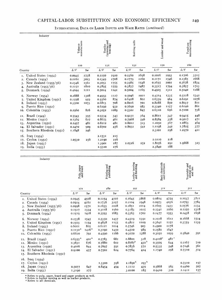
CAPITAL-LABOR SUBSTITUTION AND ECONOMIC EFFICIENCY 249
INTERNATIONAL DATA ON LABOR INPUTS AND WAGE RATES (continued)
Industry
.0~~~~~~~~b
220 231 232 250 260
Country LIV $W LIV $W LIV $W LIV $W LIV $W
I. United States (I954) 0.0945 2738 0.2250 2920 0.2360 2698 0.2026 2993 0.I706 35I5
2. Canada (I954) o.ii6I 3023 0.2349 2708 0.2779 2260 0.2I7I 2546 0.2385 2668
3. New Zealand (I955/56) 0.2346 I562 0.3053 I755 0.3985 I548 0.2655 2002 0.3678 I834
4. Australia (I955/56) 0.225I i8io 0.3895 I559 0.3837 I487 0.35I7 I794 0.3857 I7I3
5. Denmark (Ig54) 0.4044 I2II 0.5024 I242 0.5004 II6g 0.4905 I3I2 0.5040 I288
6. Norway (1954) 0.2888 I308 0.4993 I127 0.5046 I02I 0.47I4 I335 0.5228 I342
7. United Kingdom (1951) 0.2598 959 o.5560 874 o.6408 802 o.6359 964 0.629I I078
8. Ireland (I953) 0.3500 I073 0.68I3 708 o.8oi6 70I o.8288 850 o.8037 8ii
9. Puerto Rico (1952) 0.6290 932 0.7690 983 0.3340 II57 o.6240 86i
io. Colombia (I953) 0.2960 826 0.3052 i089 0.5302 845 0.63I0 696 0.7200 738
II. Brazil (I949) 0.5943 395 0.9334 343 0.923I 364 o.86II 347 0.94I5 448
I2. Mexico (I95I) O.I369 627 o.8673 46I 0.7968 546 o.8584 358 0.90I7 471
I3. Argentina (1950) 0.2497 48I 0.82I2 48I 0.80I2 523 I.2050 367 I.0863 464
14. El Salvador (I95I) 0.2470 909 o.8702 456 o.8032 542 I.II98 342 I.7825 377
I5. Southern Rhodesia (I952) I.I848 246 2.320I 298 I.2970 42I
i6. Iraq (1954) 2.I53I 215
17. Ceylon (1952) I.0530 256 1.2190 226 2.0220 228
i8. Japan (1953) 1.3901 287 2.0526 252 i.8o56 292 I.9668 323
I9. India (Ig53) 2.5320 276 2.3840 I88
Industry
bO cn c t
n~~~~~~~~~b a1 = c S i2
27I 280 29I 3II 3-2
Country L/V $w L/V $cw L/V $cw L/V $c L/V $cw
I. United States (I954) 0.0945 4508 O.I254 4507 O.I645 3868 0.08I4 4754 0.1037 382I
2. Canada (I954) 0.0924 4262 O.I736 3297 0.2I04 2948 0.0973 4036 0.0793 3784
3. New Zealand (I955/56) o.o998 2570 0.2655 2008 0.285I 20I4 O.I603 2433 O.I576 2234
4. Australia (I955/56) O.I927 2334 0.3II8 I960 0.3283 2025 0.234I 2060 O.I250 23I8
5. Denmark (I954) 0.25I9 I428 0.3593 I683 0.3363 I702 0.2477 I553 0.2438 I698
6. Norway (1954) 0.2338 I545 0.5350 I457 0.45I9 I39I 0.2028 I6I2 0.2668 I524
7. United Kingdom (1951) 0.2503 II54 0.4838 II55 0.4822 II09 0.364I I25I 0.3559 I239
8. Ireland (I953) o.6ooi 805 0.622I I024 0.5746 903 0.4900 II78
9. Puerto Rico (1952) 0.II30a I426a 0.3I90 I450 0.45I0 989 0.2580 I647
io. Colombia (I953) o.6820 792 0.4590 ii66 0.3070 I388 0.3050 I039 0.5840 59I
ii. Brazil (I949) o.6355a 402' 0.5783 682 o.88oo 328 0.4208c 48I c
I2. Mexico (I95I) 0.383I 676 0.7880 602 o.8787b 43ob 0.3509 644 0.2I67 7I0
13. Argentina (I950) 0.40I6 644 0.7697 59I 0.7836 572 0.5335 548 0.7I46 56i
I4. El Salvador (9s5) 0.9200 457 0.7502 624 0.7764 424 I.I740 298 0.73I0 3I4
i5. Southern Rhodesia (1952)
i6. Iraq (I954)
I7. Ceylon (1952) 1.3300 398 2.I8gOb 293b 0.73I0 197
i8. Japan (I953) 0.5077 647 o.8454 494 I.III2 439 o.5868 563 0.4460 507
I9. India (953) I.3I90 277 3.0I00 i85 0.94IO 320 2.2422 I57
a Refers to pulp, paper, board and paper products as well. b Refers to leather tanning as well as leather products.
Refers to all chemicals.
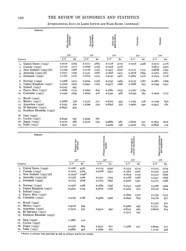
250 THE REVIEW OF ECONOMICS AND STATISTICS
INTERNATIONAL DATA ON LABOR INPUTS AND WAGE RATES (continued)
Industry
0~~~~~~ 0~~~~~~~~~~~~~~~
00&. Cd
3I9 331 332 333 334
Country LIV $W LIV $w LIV $c LIV $w L/V $w
I. United States (I954) 0.0720 4509 0.I7I2 3669 O.I2 28 4179 0.I958 3408 0-0752 42i6 2. Canada (iI954) 0.II20 3377 o.i6o6 3I98 O.I926 3370 o.o635 39I0 3. New Zealand (1955/56) 0.2I8g I906 0.2I26 2I36 0.2457 2036 0.3I72 I775 o.o686 2503 4. Australia (I955/56) O.I87I 1790 0-335I 2066 0.2856 1932 0.3828 1894 0.2562 207I 5. Denmark (I954) 0.2765 I575 0.4629 I329 0-4I42 I416 0.4883 I320 0.2034 I738
6. Norway (I954) 0.2468 1473 0.5024 I358 0-3742 1484 0.5I55 II87 0.288I 1569 7. United Kingdom (1951) 0.3600 I059 0.594I II09 0.5477 io68 0.7666 835 0.2394 I43I 8. Ireland (I953) 0.4745 943 9. Puerto Rico (1952) o.i68o I554 0.2800 8oo o.568o I79 0.7260 II84
io. Colombia (I953) 0.2740 I094 I.0630 5I6 0.3290 968 o.6740 783 0.2040 I227
I I. Brazil (I949) I2. Mexico (I95I) 0.3668 748 I-7452 32I o.6707 493 I.2285 328 0.2709 630 13. Argentina (1950) 0.5I93 570 1.5700 370 o.8646 570 I.0480 440 0.5443 58I 14. El Salvador (I95I) o.6830 429
Is. Southern Rhodesia (1952)
i6. Iraq (1954)
17. Ceylon (1952) o.8340 293 1.9340 I67 I8. Japan (1953) 0.5270 486 2.5310 274 o.9660 467 i.8700 331 o.i693 I025 I9. India (Ig53) I.0970 337 5.4400 I46 3.0470 229 o.8890 3I9
Industry
cS. 0 4 c
341 342 350 370
Country LIV $co LIV $W LIV $c LIV $w
I. United States (954) 0.1266 4387 O.III9 4540 O.I332 4314 0-I3I4 4II9 2. Canada (Ig54) O.I4I0 3769 0.0768 3955 O.I562 3507 0.1579 3536 3. New Zealand (I955/56) 0.2340 2I90 0.2639 2I90 0.3I22 I856 4. Australia (1955/56) 0.2338 2306 0.235I 2I94 0.3268 I966 0.343I I898 5. Denmark (Ig54) 0.2I73 I656 O.I775 I695 o.4006 144I 0.4272 I466
6. Norway (I954) 0.29I8 1568 0.2684 I648 0-4I42 1438 0.3266 I489 7. United Kingdom (195I) 0.4503 I224 0.3870 1208 0.5464 979 0.6226 1024 8. Ireland ( 953) 9. Puerto Rico (1952) 0.2800 1307 0.I370 1535
io. Colombia (I953) 0.4199 ii68 0.4560 I526 o.5640 879 0.4270 972
II. Brazil ('949) 0.5350 572 I2. Mexico (I95I) 0.4728 594 0.5580 455 0.5537 643 I3. Argentina (1950) 0.7920 59I 0.5512 542 o.8747 463 o.6826 6I9 I4. El Salvador (I95I) 2.7322 243 I5. Southern Rhodesia (1952)
i6. Iraq (I954) I.2866 2I0 I7. Ceylon (1952) i8. Japan (1953) 0.7256 664 0.5432 62I I.2388 422 o.8054 5I7 I9. India (Ig53) o.9860 450 2.2000 262 I-7I70 306
d Refers to primary iron and steel as well as primary non-ferrous metals.