capturing the uncertainty of moving-object representations

Capturing the Uncertainty of Moving-Object

Representations

Dieter Pfoser and Christian S. Jensen

Department of Computer Science, Aalborg University, DENMARK{pfoser|csj}@cs.auc.dk

Abstract. Spatiotemporal applications, such as fleet management andair traffic control, involving continuously moving objects are increasinglyat the focus of research efforts. The representation of the continuouslychanging positions of the objects is fundamentally important in these ap-plications. This paper reports on on-going research in the representationof the positions of moving-point objects. More specifically, object posi-tions are sampled using the Global Positioning System, and interpolationis applied to determine positions in-between the samples. Special atten-tion is given in the representation to the quantification of the positionuncertainty introduced by the sampling technique and the interpolation.In addition, the paper considers the use for query processing of the pro-posed representation in conjunction with indexing. It is demonstratedhow queries involving uncertainty may be answered using the standardfilter-and-refine approach known from spatial query processing.

1 Introduction

A relatively new research area, spatiotemporal databases concerns the man-agement of objects with spatiotemporal extents, and real-world objects withcontinuously changing spatial extents are attracting substantial attention. Thevariety of applications suggests that there is not just one prototypical type ofspatiotemporal application.

Spatiotemporal applications may be distinguished based on the data theymanage, which may pertain to the past, the present, and the future, or a com-bination of these. For example, applications managing past data often conductanalyses of movements over time, answering queries such as, “What were themovements of the Vikings in the North Sea between year 1000 and year 1200?”Applications dealing with present and future data capture the current spatial ex-tents of objects in the database and typically make predictions about the futureextents of the objects. Sample queries include, “What is the position of flightSAS 286?” and “Where will flight SAS 286 be in 20 minutes?” Next, a specifictype of application concerns real-world objects that move continuously and dis-regards the spatial extents of the objects, representing instead their positionsas points. Candidate applications include fleet management, air traffic control,military command-and-control systems, and people tracking. This paper focuses

R.H. Guting, D. Papadias, F. Lochovsky (Eds.): SSD’99, LNCS 1651, pp. 111–131, 1999.c© Springer-Verlag Berlin Heidelberg 1999

LNCS 1651, pp111-131, May 1999.(URL: http://www.springerlink.com/link.asp?id=2tkkptp0yxeadqdf)Copyright © Springer-Verlag

112 Dieter Pfoser and Christian S. Jensen

on the representation of the past and present positions of such moving-pointobjects.

Fundamental issues in these applications include the acquisition and repre-sentation of the movements of objects, including the inherent imprecision in therepresentation. For example, when representing the positions of vehicles based onsampling, the sampled positions are inherently imprecise, as are the interpolatedpositions in-between the samples. As a result, the record of the movements ofobjects as stored in the database differs from the actual movement. The impreci-sions due to the measurements and caused by the use of sampling are inherentlyquite different. It is highly relevant to understand the nature of these impreci-sions because this makes it possible to decide on their relative importance.

This paper’s contributions are three-fold. First, it offers a proposal for repre-senting the positions of moving-point objects in databases. Second, it quantifiesthe imprecisions in the proposed representation. The representation is modular,allowing the imprecision to be captured or not, depending on the applicationrequirements. Third, the paper illustrates how the representation may be usedin conjunction with indices to answer queries involving uncertainty. The two-step filter-and-refinement process known from spatial query processing is usedtogether with error information.

Past database research has focussed on spatiotemporal applications whereonly the present and future positions of moving-point objects are relevant. Inthe context of applications that predict the movements of objects based on theircurrent positions, speeds, and directions, Wolfson et al. (16) address positionupdate policies and the imprecision involved in the database-representation ofthe positions. Next, Moreira et al. (9) present a data model for moving-pointobjects that is based on the decomposition of the trajectories of the objectsinto sections. In addition, so-called superset and subset semantics are proposedthat aim to address uncertainty issues. A maximum error occurs when linearlyapproximating the movement of an object in-between samples, and this erroris used in the process of query processing. However, this work is not connectedto any specific application or technological context and thus does not cover theranges of errors and the relationships between different error measures. Thequery processing aspects also do not consider the availability of indices. Gutinget al. (5) present a comprehensive framework of abstract data types for movingobjects. This work, however, does not address representation issues, nor does itaccommodate uncertainty.

The outline of the paper is as follows. Section 2 presents an application sce-nario and describes a particular technological context for the application, theGlobal Positioning System. Section 3 proceeds to describe, quantify, and relatethe measurement and the sampling errors in the context of the application sce-nario and accommodates also error information in the representation. This setsthe stage for a proposal for a database representation for moving-point objects,presented in Section 4. Section 5 considers the utilization of this representation inquery processing using indices. Finally, Section 6 concludes and offers directionsfor future research.

Capturing the Uncertainty of Moving-Object Representations 113

2 An Application Scenario—GPS-Based FleetManagement

This section presents a sample spatiotemporal application scenario, fleet man-agement, and briefly introduces the Global Positioning System (GPS), the tech-nology that is assumed used for sampling the positions of moving objects.

2.1 Fleet Management

The optimization of transportation, especially in highly populated areas, is a verychallenging task that may be supported by an information system. An examplefleet management project, conducted by the Department of Transportation ofthe State of California, Caltrans (3), aims to design what is termed the AdvancedTransportation System. In this application, vehicles equipped with GPS devicestransmit their positions to a central computer using either radio communicationlinks or cellular phones. At the central site, the data is processed and utilized.Example queries occurring in such an application are as follows.

– Which taxi is closest to customer A?– What is optimal taxi distribution over the area (somewhat related to pickups

per area)?– Compute the optimal route for a ride, considering road characteristics such

as the actual and theoretical speed limits, congestions, accidents, etc.

Taking uncertainty into account, more sophisticated queries may be formulated.

– Which taxis were, with a 50% probability, within 100 meters of the Ritzhotel at 14.20 on April 22, 1999?

– How likely is it that taxi 1234 had visual contact with (was within 100 metersof) taxi 4321 between 9.00 and 13.00 on April 22, 1999?

– Which taxis were with 50% probability in Central Park at 10.00 on April22, 1999.

2.2 Global Positioning System

The Global Positioning System is able to determine exact positions on Earthanytime, in any weather, and anywhere. The system consists of 24 satellites thatorbit Earth at 20000 km. The satellites transmit signals that can be detectedby GPS receivers, which then are able to determine their locations with greatprecision.

The principle behind the GPS is the measurement of the distances betweena receiver and several satellites. A total of four distances, and thus signals fromfour satellites, are needed to solve a set of four equations that expresses thelatitude, longitude, height, and time (Magellan Corporation 8). The distancefrom the satellite to the receiver can be calculated by multiplying the time ittakes for the signal to arrive by the speed at which it travels–the speed of light.


Although four visible satellites are enough to compute a position, the moresatellites that are visible, the more precise the computed position becomes.

More information about the GPS can be found in, e.g., Magellan Corporation(8) and Leick (7).

3 Sampling and Uncertainty

This section covers how to acquire and represent the movement of point objects.We first give the technical means of how to determine the time-varying positionsof moving point objects, and subsequently give a suitable way to represent theentire movement. An important part of the representation is the uncertaintycaused by the acquisition process. The section describes the uncertainty causedby the measurement error and the sampling error, and it concludes with a dis-cussion of the relative importance of these errors.

3.1 Acquiring Movement—Measuring Position in Time

In order to record the movement of an object, we would have to know the positionat all times, i.e., on a continuous basis. However GPS and telecommunicationstechnologies only allows us to sample an object’s position, i.e., to obtain theposition at discrete instances of time such as every few seconds.

The solid line in Fig. 1(a) represents the movement of a point object. Space(x and y axes) and time (t axis) are combined to form one coordinate system.The dashed line shows the projection of the movement in two-dimensional space(x and y coordinates).

A first approach to represent the movements of objects would be to store theposition samples. For our database, this would mean we could not answer queriesabout the objects’ movements at times in-between sampled positions. Rather,to obtain the entire movement we have to interpolate. The simplest approachis to use linear interpolation, as opposed to other methods such as polynomialsplines (Bartels et al. 1). The sampled positions then become the end points ofline segments of polylines, and the movement of an object is represented by anentire polyline in three-dimensional space. In geometrical terms, the movementof an object is termed a trajectory (we will use “movement” and “trajectory”interchangeably).

Fig. 1(b) shows the spatiotemporal space (the cube in solid lines) and severaltrajectories (the solid lines). Time moves in the upward direction, and the top ofthe cube is the time of the most recent position sample. The wavy-dotted linesat the top symbolize the growth of the cube with time.

3.2 Quantifying Uncertainty

The research on uncertainty in geospatial information is concerned with allsources of incorrectness and incompleteness in the measurement, analysis, andinterpretation of digitally-represented, Earth-referenced phenomena (Unwin 13).


time y

x

1tt

4

5

0

2

3

t

t

t

t

movement

(a) Trajectory of a moving point

��

�

��

��

�

��

�

��

��

��

��

��

��

��

��

��

�

��

�

��

�

��

�

��

��

��

��

��

��

��

�

��

��

��

inital statetimey

x

last recorded state

(b) A spatiotemporal space

Fig. 1. Movements and spaces

A representation of moving-point trajectories is inherently imprecise: impre-cision is introduced by the measurement process used in the sampling of positionsand by the sampling approach itself. A useful representation of moving pointsmust take these uncertainties into account.

In this paper, we make the following assumptions.

– We will not consider any error connected to the times of measurements. Weassume that we know precisely the time a position sample was taken. Thisassumption seems to be justified when using the GPS and its precise clocksas a measuring device.

– Within one application, we will only consider objects with similar movementcharacteristics, such as speed and range. Typical examples of objects withdifferent characteristics include people, cars, and planes.

A first step in incorporating uncertainty into a representation of trajectories is toquantify it. We thus proceed to describe the errors introduced by the trajectoryacquisition process.

3.3 Measurement Error

Generally, an error can be introduced by inaccurate measurements (Leick 7).The accuracy and thus the quality of the measurement depends largely on thetechnique used. This paper assumes that the GPS is used for the sampling ofpositions.

Two assumptions are generally made when talking about the accuracy of theGPS. First, the error distribution, i.e., the error in each of the three dimensionsand the error in time, is assumed to be Gaussian. Second, we can assume thatthe horizontal error distribution, i.e., the distribution in the x-y plane, is circular(van Diggelen 14).

The error in a positional GPS measurement can be described by the prob-ability function in Equation (1). The probability function is composed of twonormal distributions in the two respective spatial dimensions. The mean of thedistribution is the origin of the coordinate system. Fig. 2 visualizes the errordistribution. In addition to the mean, the standard deviation, σ, is a character-istic parameter of a normal distribution . Within the range of ±σ of the mean,


in a bivariate normal distribution (2-dimensional), 39.35% of the probability isconcentrated.

P1(x, y) =1

2πσ2e−

x2+y2

2σ2 (1)

circular positional error

x

y

probability

Fig. 2. Positional error in the GPS

Example 1. A typical GPS module used in vehicle navigation systems is theCrossCheck AMPS Cellular from Trimble Navigation Ltd. This GPS/cellularphone system has an error of 2m (equal to 1 σ) (Trimble Navigation Ltd. 12).This measure refers to the standard deviation of a bivariate normal distributioncentered at the receiver’s true antenna position.

3.4 Uncertainty in Sampling

We capture the movement of an object by sampling its position using a GPSreceiver at regular time intervals. This introduces uncertainty about the positionof the object in-between the measurements. In this section, we give a model forthe uncertainty introduced by the sampling, based on the sampling rate and themaximum speed of the object.

Sampling Error The uncertainty of the representation of an object’s movementis affected by the frequency with which position samples are taken, the samplingrate. This, in turn, may be set by considering the speed of the object and thedesired maximum distance between consecutive samples. Let us consider therunning example, in which we want to record the movements of taxis.

Example 2. As a requirement to the application, the distance between two con-secutive samples should be maximally 10 meters. If the maximum speed of a taxiis 150km/h, this means that we would need to sample the position at least 4.2times per second. If a taxi moves slower than its maximum speed, the distancebetween samples is less than 10 meters.

We proceed to consider how the position samples resemble the true movement ofthe object. Consider the three trajectories shown in Fig. 3. Each is possible giventhe three measured positions P1 through P3. However, by just “looking” at the


P PP1 2 3

Fig. 3. Possible trajectories of a moving object

three positions, one would assume that the straight line best resembles the actualtrajectory of the object. Since we did not measure the positions in-between twoconsecutive position samples, the best we can do is to limit the possibilities ofwhere the moving object could have been. We have to constrain the trajectory ofthe object by what we know about the object’s actual movement. Considering thetrajectory in a time interval [t1, t2], delimited by consecutive samples, we knowtwo positions, P1 and P2, as well as the object’s maximum speed, vm; see Fig. 4.If the object moves at maximum speed vm from P1 and its trajectory is a straightline, its position at time tx will be on a circle of radius r1 = vm(t1 + tx) aroundP1 (the smaller dotted circle in Fig. 4). Thus, the points on the circle representthe furthest away from P1 the object can gotten at time tx. If the object’s speedis lower than vm, or its trajectory is not a straight line, the object’s position attime tx will be somewhere within the area bounded by the circle of radius r1.Next, we know that the object will be at position P2 at time t2. Thus, applying

��

��

1 2r r

P (x , y , t )2 2 21 1 1 1P (x , y , t ) 2

Fig. 4. Uncertainty between samples

the same assumptions again, the object’s position at time tx is on the circle withradius r2 = vm(t2 − tx) around P2. If the object moves slower or its trajectoryis not a straight line, it is somewhere within the area bounded by this circle.

The above constraints on the position of the object mean that the objectcan be anywhere in the intersection of the two circular areas at time tx. Thisintersection is shown by the shaded area in Fig. 4, and we use the term lens


for this intersection. Since we do not have any further information, we assume auniform distribution for the position within the lens.

Thus, the sampling error at time tx for a particular position can be describedby the probability function shown in (2), where r1 and r2 are the two radiidescribed above, s is the distance between the measured positions P1 and P2,and A denotes the area of the intersection of the two circles.

P2(x, y) ={

1A for x2 + y2 ≤ r2

1 ∧ (x− s)2 + y2 ≤ r22

0 otherwise (2)

Substituting vm(t1 + tx) and vm(t2− tx) for the radii r1 and r2, respectively, theprobability function shown in Equation (3) results. Its parameters are describedin Table 1.

P2(x, y) =

1A for x2 + y2 ≤ (vm(t1 + tx))2∧

(x − s)2 + y2 ≤ (vm(t2 − tx))2

0 otherwise(3)

For a visualization of a sampling error, refer to Fig. 5(a), in which the twohorizontal axes depict x and y coordinates, and the vertical axis the positionalprobability.

Table 1. Parameters of the probability function, P2, describing the samplingerror

vm maximum speed of the moving objecttx time for which the error distribution is computedt1 time of the first measured positiont2 time of the second measured positions distance between the two positions, i.e., the length of the line segmentA lens area, i.e., the area of the intersection of the two circles

-10

-5

0

5

10 -10

-5

0

5

10

0

0.01

0.02

0.03

0.04

10

-5

0

5

(a) Normal-case sampling error

-10

0

10

-10

0

10

0

0.001

0.002

0.003

-10

0

10

(b) Worst-case sampling error

Fig. 5. Probability functions for sampling errors

Sampling Error Across Time So far, we have quantified the sampling errorfor the position at a single point in time. To determine the error across time, as afirst step, we compute the lens for various tx ∈ [t1; t2] as shown in Figs. 6(a)–(c).


The circle around the first point, P1, measured at time t1, is initially a pointand grows as time advances, and the circle around the second point, P2, shrinkswith the advancement of time and eventually becomes a point. In the first situa-tion in Fig. 6(a), the circle around P2 contains the one around P1, meaning thatthe constraint on how far away the object can be from P1 at tx is more restrictivethan the constraint on how close it has to be to P2. The area of intersection isthe total circle or radius r1. In the second situation, Fig. 6(b), the two circlesstart intersecting, and in Fig. 6(c) they show a clear intersection.

We observe that the intersection points of the two circles over time, i.e., forthe cases the circles do actually intersect, lie on an error ellipse with positions P1

and P2 as its foci (cf. Fig. 7). The length of the semi-major axis is 2a = r1 + r2.This is not surprising if we consider the definition of an ellipse. An ellipse is

(a) (b) (c)

Fig. 6. Evolving sampling error

��

2a

2c

2b

s

s

sP (x , y , t )1 1 1 1 2P (x , y , t )2 22

max

max

Fig. 7. Error ellipse

a curve consisting of all points in the plane whose sum of distances, r1 and r2,from two fixed points, P1 and P2 (the foci) separated by a distance of 2c, is agiven constant, 2a. The measure 2c can be interpreted as the observed distancebetween P1 and P2, whereas 2a is the maximum distance the object can travel.The “thickness” of the ellipse, 2b, is determined by the equation b2 = a2 − c2.


This means that the smaller the difference between the observed distance, 2c,and the maximum distance, 2a, the “thinner” the ellipse. In the extreme case,the ellipse degrades to a line segment. In the worst case, where the object doesnot move between consecutive position samples, the ellipse becomes a circle.

Sampling Rate Having derived the general principle behind the sampling error,we give an example of how an increased sampling rate affects the error size. Toillustrate the underlying principle, we use the error ellipse given in Fig. 7 as ameasure for the size of the sampling error per line segment.

Example 3. In Fig. 8, we show the actual trajectory of a moving object as abold line. As a first step, we sample the movement of the object at position P1

and P2. The time in-between the samples is 10 seconds. The shortest distancefrom P1 to P2 is 300 meters. Thus, to the best of our knowledge the objecttravels at a speed v of 30m/s. If we further know the maximum speed of theobject to be 42m/s, we can draw an error ellipse around the line approximatingthe movement. The error ellipse has an eccentricity 2c = 300m, a major axis2a = vmax ·∆t = 42m/s×10s = 420m, and a minor axis 2b =

√(2a)2 − (2c)2 =√

4202 − 3002 = 294m. This rather large error ellipse means that the position ofthe object in-between samples is quite uncertain. Quadrupling the sampling rate,i.e., sampling the position every 2.5 seconds, leads to an error ellipse that hasan eccentricity 2c = 80m, a major axis 2a = vmax ·∆t = 42m/s× 2.5s = 105m,and a minor axis 2b =

√(2a)2 − (2c)2 =

√1052 − 802 = 68m.

sampling rate: r

sampling rate: 4 x rP3

1P4

P

PP

5

2

Fig. 8. Varying sampling rate

If we increase the sampling rate, the sample positions better approximate themovement, and the error introduced by sampling is decrease.

Maximum Speed Challenged An underlying assumptions so far has been that themaximum speed of a moving object is fixed at vmax. However, the more we knowabout the object in question, the further we can narrow down vmax and thus


reduce the uncertainty. For example, if we know that a taxi can reach 200km/h,but regulations of the company set 120km/h as the upper limit, we may decide toassume that vmax is 150km/h. Further examples of such additional informationare local speed limits and road conditions; thus the maximum speed can varydepending on the area the taxi is in. Traffic volumes, which are time dependent,may also be taken into account. Further, there might be individual speed limitsfor drivers and cars. Generally, the more information we have about an object,the better we can adjust the sampling rate, reduce the error, and, consequently,minimize the uncertainty attached to its polyline trajectory.

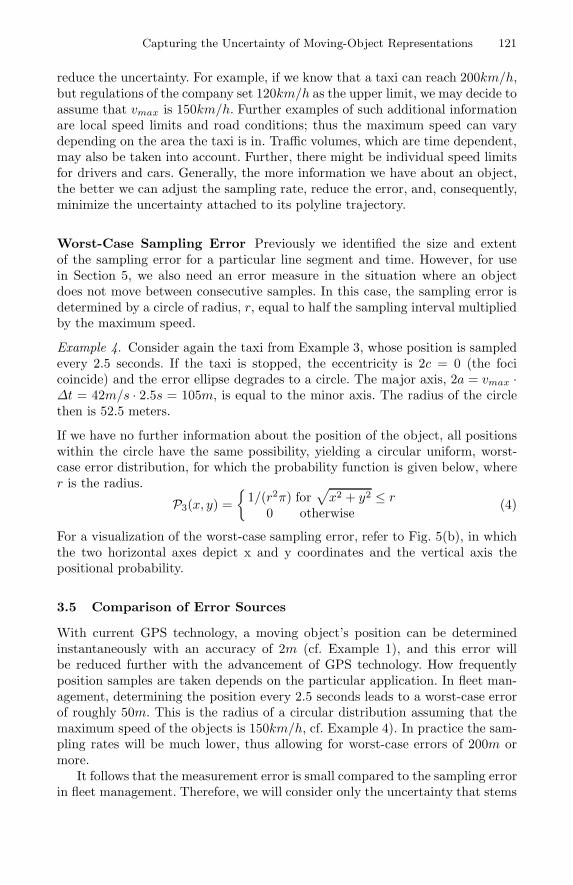
Worst-Case Sampling Error Previously we identified the size and extentof the sampling error for a particular line segment and time. However, for usein Section 5, we also need an error measure in the situation where an objectdoes not move between consecutive samples. In this case, the sampling error isdetermined by a circle of radius, r, equal to half the sampling interval multipliedby the maximum speed.

Example 4. Consider again the taxi from Example 3, whose position is sampledevery 2.5 seconds. If the taxi is stopped, the eccentricity is 2c = 0 (the focicoincide) and the error ellipse degrades to a circle. The major axis, 2a = vmax ·∆t = 42m/s · 2.5s = 105m, is equal to the minor axis. The radius of the circlethen is 52.5 meters.

If we have no further information about the position of the object, all positionswithin the circle have the same possibility, yielding a circular uniform, worst-case error distribution, for which the probability function is given below, wherer is the radius.

P3(x, y) ={

1/(r2π) for√

x2 + y2 ≤ r0 otherwise

(4)

For a visualization of the worst-case sampling error, refer to Fig. 5(b), in whichthe two horizontal axes depict x and y coordinates and the vertical axis thepositional probability.

3.5 Comparison of Error Sources

With current GPS technology, a moving object’s position can be determinedinstantaneously with an accuracy of 2m (cf. Example 1), and this error willbe reduced further with the advancement of GPS technology. How frequentlyposition samples are taken depends on the particular application. In fleet man-agement, determining the position every 2.5 seconds leads to a worst-case errorof roughly 50m. This is the radius of a circular distribution assuming that themaximum speed of the objects is 150km/h, cf. Example 4). In practice the sam-pling rates will be much lower, thus allowing for worst-case errors of 200m ormore.

It follows that the measurement error is small compared to the sampling errorin fleet management. Therefore, we will consider only the uncertainty that stems


from the sampling, and disregard the uncertainty caused by the measurementtechnique, in the remainder of the paper.

4 A Representation for Moving Point Objects

Section 3 proposed a technique for capturing the movement of point objectsthat utilized polylines, and the section characterized the error introduced bythis technique, this way also revealing the uncertainty inherent to the polylinerepresentation. This section’s objective is to provide a format for representingthe history of the positions of continuously moving point objects, along with theuncertainty associated with our records of their positions. For this, we proposea relational database schema that incorporates all the spatiotemporal and errorinformation previously presented in this paper.

Specifically, the schema in Table 2 defines relations for objects, for the linesegments constituting the trajectories of the objects, and for the error informa-tion associated with the recorded trajectories. Relation Object has attributes

Table 2. Relational schema for capturing moving-point objects, their trajecto-ries, and associated error information

Object < object id, max speed, etc. >Line segment < line id, object id, t1, t2, x1, x2, y1, y2, error id >Error < error id, error type, param1, param2 >

object id, which is the key attribute, and max speed, which determines themaximum speed at which the object can move. In addition this relation mayinclude any number of attributes unrelated to the objects’ spatial extents. Re-lation Line segment captures the line segments that compose the trajectoriesof the objects. Attribute line id is the key attribute; object id is a foreign keyreferencing relation Object; and t1 and t2 are the times when the two positions,(x1, y1) and (x2, y2), constituting the line segment, were measured. Finally, re-lation Error contains the error information associated with the line segments.Attribute error id is the key; error type specifies the type of error that a tuplerefers to, and thus specifies how parameters param1 and param2 are to be in-terpreted. In the current schema, there is only one type of error. However, if weconsider more error sources in our application, additional types of errors mayoccur.

The domains of the attributes are as follows. Define dom(x) to be a functionthat returns the domain of its argument attribute x. Then dom(object id) =dom((line id) = dom(error id) = dom(max speed) = dom(t1) = dom(t2) = N ,where N is the natural numbers, dom(param1) = dom(param2) = N ∪ NIL,dom(x1) = dom(x2) = dom(y1) = dom(y2) = Z, where Z is the integers, anddom(error type) = {worst-case sampling}.

The following example illustrates how the above schema can be put to use.


Example 5. Our taxi company operates a number of taxis in a city. The databasein Fig. 9 captures the movement of the taxis together with the associated errors.

This database permits the company to reconstruct the trajectories of itstaxis and to compute the associated error information. All taxis are recordedin relation Object, and their trajectories are kept in Line segment and arereferenced through the foreign key object id.

Objectobject id max speed

1234 1204321 1501235 140

...(a)

Line segmentline id object id error id t1 t2 x1 x2 y1 y2

1 1234 1 . . .2 1234 1 . . .3 4321 1 . . .

...(b)

Errorerror id error type param1 param2

1 worst-case sampling 25 NIL

(c)

Fig. 9. An example database containing positional and error information con-nected to a fleet management application of a taxi company

To utilize the error information, the parameters for the various probabilityfunctions are recorded. The parameter of the worst-case sampling error, P3, isthe radius r, which in our database is stored as the param1 attribute value (25)of the only tuple in relation Error.

The parameters of the sampling error, P2, as shown in Table 1, are thedistance s, which is computed from the attribute values for x1, x2, y1, and y2

in relation Line segment, together with the times t1, and t2. The maximumspeed vm is stored in relation Object. Finally, tx is not a static parameter thatcan be stored in a relation, but is an input parameter from a query. Thus, theintersection area A, which is different for each position in time contained in aparticular line segment, can also only be computed once tx is known.

5 Query Processing and Indexing

The objective of this section is to explore the use of error information when usingindices for processing queries involving the positions of moving objects. Thesection first sets the context within spatiotemporal indexing for its contribution.Subsequently, it shows how a moving-point index may be put to use in theprocessing of spatiotemporal range queries involving positional uncertainty. Adiscussion of what types of queries that can be answered in the given frameworkis given. The section ends with a summary of the section’s proposed approach.


5.1 Context

The purpose of spatiotemporal indexing is to efficiently support the retrievalof those objects, from a large set of objects, with spatiotemporal extents thatsatisfy a specified query predicate. The most commonly considered predicate isintersection with a specified region.

Substantial research is currently ongoing in spatiotemporal indexing, and anumber of spatiotemporal indices have already been proposed; see Theodoridiset al. (11) for an overview. Although an index well suited for indexing the tra-jectories of the kinds of moving-point objects considered here still does not exist,it is expected that such an index will be invented.

In terms of the representation proposed in this paper, this means that wecan expect to be able to index the polyline segments that represent trajecto-ries. However, taking the uncertainty of the trajectories into consideration cor-responds to the indexing of (non-point) objects with spatial extents, and theenvisioned moving-point indices are no longer readily applicable.

Based on the assumption that it will be substantially more attractive to indexthe trajectories of moving-point objects than to index the trajectories of objectswith spatial extents, which are more complex, this section offers an approach tousing moving-point trajectory indices while taking into account the uncertaintyof the trajectories and also taking into account query predicates relating to theuncertainty.

The approach employs the fundamental technique from spatial indexing ofusing approximations for the spatial extents to be indexed (Guting 4). For in-stance, R-trees generally use minimum bounding boxes. This use leads to a filter-and-refine strategy for query processing. First, based on the approximations, afiltering step is executed that returns a superset of the objects fulfilling the querypredicate. Second, in the refinement step, the exact extents of the objects re-sulting from the first step are checked against the query predicate (Brinkhoff etal. 2).

5.2 Processing Uncertainty Queries

The goal here is to be able to use a moving-point index to answer queries such as“Retrieve the positions of taxis that were inside area A (specified as a rectangle)between times B and C with a probability of at least 30%?”

The first step is to specify the meaning of an object’s position being withinan area A with a probability of 30%. An object’s position is described by meansof a probability function centered around the positional mean (e.g., recall theprobability function of the worst-case sampling error in Fig. 5(b)).

If all of an object’s positional probability is within an area A, we say thatthe object is within area A for certain. We can determine if this is the case byintegrating over the probability function with area A as the limit. If the resultis 1, this is the case.

If the object is within area A with a probability of at least 30%, at least 30%positional probability has be concentrated within area A. This case is shown in


Fig. 10, where the circle represents the probability function of the worst-casesampling error, the rectangular shape is the query rectangle, and the shadedregion represents the probability in the query window. The result of integratingover the probability function with rectangle A = ([xmin, xmax], [ymin, ymax]) asthe limit thus has to be 0.3 or higher. Further, if the positional error is rota-

measure

miny

maxy

expansion

worst-case error

query window

mean

x maxx min

Fig. 10. Summing up the probability

tionally symmetric around the positional mean, as is the case for the worst-casesampling error, we can determine the maximum distance of the query windowto the positional mean such that the probability of the position to be within thequery window is 30% or higher. We term this computed distance the expansionmeasure. In Fig. 10 this distance is indicated by the arrow from the edge of thequery window to the center of the probability function (the mean). The expan-sion measure can be interpreted as the measure by which the query window hasto be expanded to contain the positional mean (the dotted query window in thefigure).

Note that we are assuming that the query window is longer and wider than2r, the diameter of the error distribution; later in this section, we will revisit thisassumption. However, for now, we proceed to show how the expansion measurecan be used in the filter step.

The Filter Step We record the positions in time of the moving objects bymeans of line segments. The points on these segments are the mean values ofthe positional probability functions Our objective for the filter step is to retrievethose line segments that contain positions in time qualifying for the query result,i.e., those positions that, with the probability specified in the query, are in thequery window. To retrieve these line segments, we intersect the expanded querywindow with the indexed line segments. Expanding the query window meansthat all positions with a probability higher or equal the one specified in thequery (the one used to compute expansion measure) are contained in the querywindow.


For the filter step, the error measure used to determine the expansion measurecan be coarse, but has to be universal so that it applies for all positions in thedatabase. This is true for the worst-case sampling error described in Section 3.4.

As we shall see next, this method can only be applied if the probabilityspecified in the query is less than 50%.

Consider again the above query, but with a probability of 60%. Using theworst-case sampling error leads to a negative query expansion measure (cf.Fig. 11(b)). If we use this smaller query window, we would retrieve a subsetrather than a superset of the qualifying objects, since, e.g., positions that haveno error (or a small error) and lie on (or close within) the borders of the querywindow would be disregarded. An example here is position P that has no errorassociated in Fig. 11(b). Shrinking the query window by the size of the nega-tive expansion measure would eliminate this position from our set of candidatesolutions.

This problem is solved by simply using the original query window with noexpansion (shrinking) for probabilities higher than 50%. This means that weretrieve a superset of the qualifying objects.

measureexpansion

worst-case error

query window

mean

P

Fig. 11. Query window expansion: high probability

The Refinement Step To determine the final result, we have to evaluate thequery predicate on all objects identified during the filtering step. In our case wehave identified line segments that intersect with the transformed query region.As the final answer, we would like to have a set of positions, and so the refinementstep extracts those parts of the line segments that qualify for this set.

In the filter step the intersection of line segments with the query window wasdetermined with the help of the worst-case sampling error. To evaluate positionsin time in the refinement step we will use the sampling error, unique for everyposition. A very straightforward way to achieve this is to apply the brute-forcemethod of computing the probability functions in turn for all positions in timecontained in a line segment (cf. Section 3.4) and check whether at least 30%probability is concentrated within area A. Fig. 12 shows two positions in time,P1 and P2, and their respective sampling errors (depicted by dotted lines). For


each of the positions, the probability concentrated within the query windowis depicted by a shaded area. The set of solutions after the refinement step

P

P

1

2

query window

Fig. 12. Refinement step

comprises all positions in time whose positional probability within a given querywindow is at least as high as specified in the query.

On the Size of Query Windows Some query types deserve special attentionwithin the presented framework. Point queries such as “Which taxis were inlocation A (point) at time B with 50% probability?” cannot be answered withinthis framework, since we cannot compute how much probability is concentratedwithin a point.

However, some “point” queries actually might be translated into windowqueries, e.g., location A might refer to a road crossing or a waiting area fortaxis. In this case we are confronted with a small-window query.

Consider the above query where the query window of location A has an extentof, e.g., a taxi stand. If the sampling rate of the taxis’ positions was very coarse,the positions have a high degree of uncertainty, and the sampling error is verylarge. To find an answer to our query, we have to determine the positions forwhich at least 50% of the probability is concentrated within the query window.If the query window is too small with respect to the error measure, no positionswill qualify, e.g., consider query window QW1 in Fig. 13.

On Non-Empty Query Results To derive a first minimum size of a query windowfor which the result is not guaranteed to be empty, we assume the worst casefor both error and query. The largest possible error is the worst-case samplingerror. The worst case of a query is to specify 100% probability, e.g., “Whichtaxis were in location A (point) at time B with 100% probability?” The smallestsquare query window we can consider has side length 2r, the diameter of theworst-case sampling error, e.g., QW2 shown in Fig. 13. If the query window issmaller, the probability of the worst-case sampling error cannot by containedentirely within the query window any more, i.e., less than 100% probability isconcentrated within the query window, and the result is guaranteed to be empty.


r

worst-case error

QW

QW

1

2

Fig. 13. Small-window query

However, this only depicts the worst-case scenario. For query windows withside length larger than 2r, queries specifying varying degrees of uncertainty mayhave non-empty answers. If the query window is smaller and the query specifies100% probability, certain positions are eliminated because their associated erroris too large for them to be for certain (100%) in the query window. Althoughthis seems only to eliminate solutions, it has significant consequences for theuse of the worst-case error with the query window in the filter step, as will beexplained next.

The Filtering Step Revisited In the case the query window is smaller than 2r,the filtering as outlined earlier might eliminate positions that satisfy the querypredicate. Consider the example shown in Fig. 14(a). First, we determine theexpansion measure for a probability of 30% and the query window (the rectan-gle). The shaded area symbolizes the intersection of the error measure and thequery window. The size of the area corresponds to the positional probabilityconcentrated within the query window.

Using this expansion measure, however, would exclude qualifying positions,e.g., position P would be discarded in the filter step, although 30% or moreof its actual positional probability (dotted lens shape of the sampling error) isconcentrated within the query window.

To avoid the elimination of qualifying positions, we will initially expand thesides of small query windows that are smaller than 2r to be of size 2r andthen use the resulting window to determine the expansion measure as describeearlier in this section. This is illustrated in Fig. 14(b), where the probabilityconcentrated in the window of height 2r is symbolized by shading, and wherethe expansion measure is symbolized by the longer arrow. With this measure,position P will be in the set of candidate solutions. To recap, small windowqueries are addressed as follows. A query window can be arbitrarily small. Inconnection with databases considering spatial uncertainty, the size of the querywindow is also determined by the uncertainty specified in the query. Further,the “extent” of a spatial position stored in the database is determined by theassociated error measure. Consequently, when specifying a query, one has to keepall these measures in mind not to retrieve an unwantingly small result.


P

measure

worst-case error

query window

expansion

mean

error

(a)

��

P

measureexpansion

worst-case error

mean

error

query window

2r

(b)

Fig. 14. Query window expansion: small query window

5.3 Summary of Approach

Or goal for this section was to give a method of how to use a moving point-indexto process queries of the form “Retrieve the moving-object positions that wereinside query rectangle A at some time between times B and C with a probabilityof at least X%.” The trajectories are indexed using a moving point index thatsupports range queries. A superset of the qualifying positions are retrieved in afiltering step, in which we expand the query window to retrieve all line segmentscontaining positions that are in the query window with probability at least X%.The expansion is determined using probability X and the worst-case samplingerror, stored in the database.

In the refinement step, the positions contained in the retrieved line segmentsthat actually are within query rectangle A with probability at least X% areidentified. Here we use the sampling error, which is distinct for all positions. Thefollowing pseudo-algorithm summarizes the full retrieval procedure. We assumethat the diameter of the worst-case sampling error is 2r.

IF query window A has either height or width less than 2r THENIncrease the smaller side(s) to be of size 2r;

IF X < 50% THENApply query window expansion to A;

Let S contain the result of searching the index with A;Apply refinement to the line segments in S and return the resulting points;

6 Conclusions and Future Research

The paper investigates the representation of moving-point objects in databases.First, a set of queries derived from requirements to an application managingmoving-point objects is presented. The Global Positioning System is the tech-nology used for obtaining samples of the positions of these objects.

The paper proposes a method for acquiring and representing the movementsof point objects. The positions of objects are sampled at selected points in time,


and the positions in-between these points in time are obtained using interpola-tion, thus capturing the complete movement.

The representation of movements is inherently imprecise, and the paper con-siders two types of errors, the measurement error and the sampling error. Twomeasures were derived for the sampling error, one pertaining to each position intime, and a global worst-case error. It is further shown that the measurementerror can be ignored in the application context considered.

A database schema is proposed that incorporates both the polyline represen-tation of movements as well as the parameters of the various error distributionsassociated with the polyline representation. The schema is illustrated by an ex-ample database suited for the taxi management application.

Finally, the paper shows how to use this database to answer spatiotemporalqueries derived from the example application. The error information is usedin connection with an arbitrary moving-point index to answer spatiotemporalqueries using the standard filter-and-refinement process.

This work points to several directions for future research. First, for the repre-sentation of the movement, we chose to linearly interpolate in-between measuredpositions. More advanced techniques may be used for this purpose as well, e.g.,polynomial splines. Second, two types of error measures were considered, namelythe measurement error and the sampling error. Additionally manipulating themeasured positions before storing them in the database introduces another errorthat needs to be considered. Thus, generalizing the approach to an arbitrarynumber of error measures poses an interesting challenge. Third, in our workwe only consider uncertainty in the spatial dimensions (cf. Section 3.2). Thisis partly because of the high precision with respect to time of the positionalmeasurement device, GPS, we use. Using motion sensors or other techniquesinstead poses the question of quantifying uncertainty with respect to time aswell. Fourth, one of the underlying assumptions in our work is that objects arenot restricted in their movements through space. In reality, the space consideredwill typically contain roads, railroad tracks, walls, floors, mountains, lakes, orother “infrastructure” that facilitate or inhibit movement. This infrastructuremay be taken into account to yield a reduced overall uncertainty and error inthe database, as well as other benefits.

Acknowledgements

This research was supported in part by the CHOROCHRONOS project, fundedby the European Commission, contract no. FMRX-CT96-0056, by the DanishTechnical Research Council through grant 9700780, and by the Nykredit Corpo-ration.

The Mathematica software package (Wolfram 15) was used to compute theprobability functions shown in Figs. 5(a) and (b).


References

Bartels, R. H., Beatty, J. C., and Barsky, B. A.: An Introduction to Splines for Use inComputer Graphics & Geometric Modeling. Morgan Kaufmann Publishers, Inc.,1987.

Brinkhoff, T., Kriegel, H. P., and Seeger, B.: Efficient Processing of Spatial Joins UsingR-trees. SIGMOD Record, 22(2):237–246, 1993.

Caltrans New Technology and Research Program. Advanced Transportation SystemsProgram Plan. URL: <http://www.dot.ca.gov/hq/newtech/nt page.html>.

Guting, R. H.. An Introduction to Spatial Database Systems. VLDB Journal, 3:357–399, 1994.

Guting, R.H., Bohlen, M., Erwig, M., Jensen, C. S., Lorentzos, N. A., Schneider, M.,and Vazirgiannis, M.: A Foundation for Representing and Querying Moving Ob-jects. Technical Report, Informatik-Bericht 238, FernUniversitat Hagen, Germany,1998.

Greenwalt, C. R. and Shultz, M. E.: Principals of Error Theory and CartographicApplications. Technical Report, ACIC Technical Report No. 96, Aeronautical Chartand Information Center, St. Louis, MO, 1962.

Leick, A.: GPS Satellite Surveying. John Wiley & Sons, Inc., 1995.Magellan Corporation, The : About Global Positioning - the Basics of GPS and

GLONASS. URL: <http://www.ashtech.com/Pages/gpsndx.html>.Moreira, J., Ribeiro, C., and Saglio, J.: Representation and Manipulation of Mov-

ing Points: An Extended Data Model for Location Estimation. Cartography andGeographical Information Systems, to appear.

Nascimento, M. A., Silva, J. R. O., and Theodoridis, Y.: Access Structures for MovingPoints. Technical Report TR-33, TIMECENTER, Aalborg University, Denmark,1998.

Theodoridis, Y., Sellis, T., Papadopoulos, A., and Manolopoulos, Y.: Specificationsfor Efficient Indexing in Spatiotemporal Databases. In Proceedings of the 10thInternational Conference on Scientific and Statistical Database Management, 1998.

Trimble Navigation Ltd.: CrossCheck AMPS Cellular. Product Datasheet, 1998.Unwin, D. J.: Geographical Information Systems and the Problem of Error and Un-

certainty. In Progress in Human Geography 19, 549–558, 1995.van Diggelen, F.: GPS Accuracy: Lies, Damn Lies, and Statistics. In GPS World, 5(8),

1998.Wolfram, S.: The Mathematica Book. Cambridge University Press, 1996.Wolfson, O., Chamberlain, S., Dao, S., Jiang, L., and Mendez, G.: Cost and Imprecision

in Modeling the Position of Moving Objects. In Proceedings of the FourteenthInternational Conference on Data Engineering, 1998.

capturing the uncertainty of moving-object representations

Documents