reasoning with uncertainty representations generally treat knowledge as fact knowledge and the use...
TRANSCRIPT
Reasoning with Uncertainty• Representations generally treat knowledge as fact• Knowledge and the use of the knowledge brings with it a
degree of uncertainty • how do we represent and reason with uncertainty?
• Four forms of uncertainty– unsure input
• input from user as “don’t know” or as a possibility • input is ambiguous or noisy
– knowledge itself (such as a rule) is non-truth preserving knowledge, such as with associational knowledge
– smoking can cause cancer but if you smoke, it isn’t guaranteed that you will get cancer
– incomplete knowledge such as in medical knowledge– the conclusion derived by the AI system is not positive but is
conditional such as “likely” or 80%
Monotonicity• Monotonicity – anything we conclude from given
axioms (knowledge) and input which is true must remain true even if new input (evidence) is found– the knowledge space can increase but we cannot take away
anything previously concluded
• Example: assume that person X was murdered and through various axioms about suspects and alibis, we conclude person Y committed the murder – later, if we add new evidence, our previous conclusion that Y
committed the murder must remain true– obviously, the real world doesn’t work this way – assume for instance that we find that Y has a valid alibi and Z’s
alibi was a person who we discovered was lying because of extortion)

The Closed World Assumption• In monotonic reasoning, if something is not
explicitly known or provable, then it is false• This assumption in our reasoning can easily lead to
faulty reasoning because its impossible to know everything
• How can we resolve this problem?• we must either introduce all knowledge that is required to
solve the problem at the beginning of problem solving• or we need another form of reasoning aside from
monotonic logic• so now we turn to non-monotonic logic
Non-monotonicity• Logic in which, if new axioms are introduced, previous
conclusions can change– requires updating/modifying previous proofs
• this could be very computationally costly as we might have to redo some of our proofs
• We can enhance our previous algorithms– add M before a clause meaning “it is consistent with”
• for all X: bright(X) & student(X) & studies(X,CSC) & M good_economy(time_of_graduation) job(X, time_of_graduation)
– in a production system, add unless clauses to rules• if X is bright, X is a student and X studies computer science,
then X will get a job at the time of graduation unless the economy is not good at that time
• These are forms of assumption-based reasoning
Dependency Directed Backtracking• To reduce the computational cost of non-monotonic logic,
we need to be able to avoid re-searching the entire search space when a new piece of evidence is introduced– otherwise, we have to backtrack to the location where our
assumption was introduced and start searching anew from there
• In dependency directed backtracking, we move to the location of our assumption, make the change and propagate it forward from that point without necessarily having to re-search from scratch– you have scheduled a meeting on Tuesday at 12:15 because
everyone indicated that they were available– you cannot find a room– you backtrack to the day and change it to Thursday, but you do
not re-search for a new time because you assume if everyone was free on Tuesday, they will be free on Thursday as well

Justification Truth Maintenance System• The JTMS is a graph implementation whereby each
inference is supported by evidence– an inference is supported by items that must be true (labeled
as IN items) and those that must be false (labeled as OUT items), things we assume false will be labeled OUT
when a new piece of evidence is introduced, we examine the pieces of evidence to see if this either changes it to false or contradicts an assumption, and if so, we change any inferences that were drawn from this evidence to false, and propagate this across the graph
The ABC Murder Mystery• Consider a murder with the following knowledge
– a person who stands to benefit from a murder is a suspect unless the person has an alibi
– a person who is an enemy of a murdered person is a suspect unless the person has an alibi
– an heir stands to benefit from the death of the donor unless the donor is poor
– a rival stands to benefit from the death of their rival unless the rivalry is not important
– an alibi is valid if you were out of town at the time unless you have no evidence to support this
– a picture counts as evidence– a signature in a hotel registry is evidence unless it is
forged– a person vouching for a suspect is an alibi unless the
person is a liar
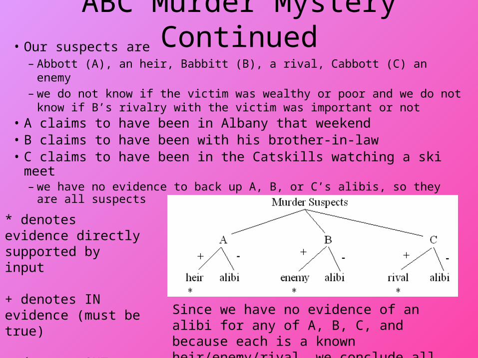
ABC Murder Mystery Continued• Our suspects are
– Abbott (A), an heir, Babbitt (B), a rival, Cabbott (C) an enemy– we do not know if the victim was wealthy or poor and we do not know if
B’s rivalry with the victim was important or not• A claims to have been in Albany that weekend• B claims to have been with his brother-in-law• C claims to have been in the Catskills watching a ski meet
– we have no evidence to back up A, B, or C’s alibis, so they are all suspects
* denotes evidence directly supported by input
+ denotes IN evidence (must be true)
– denotes OUT evidence (assumed false)
Since we have no evidence of an alibi for any of A, B, C, and because each is a known heir/enemy/rival, we conclude all three are suspects
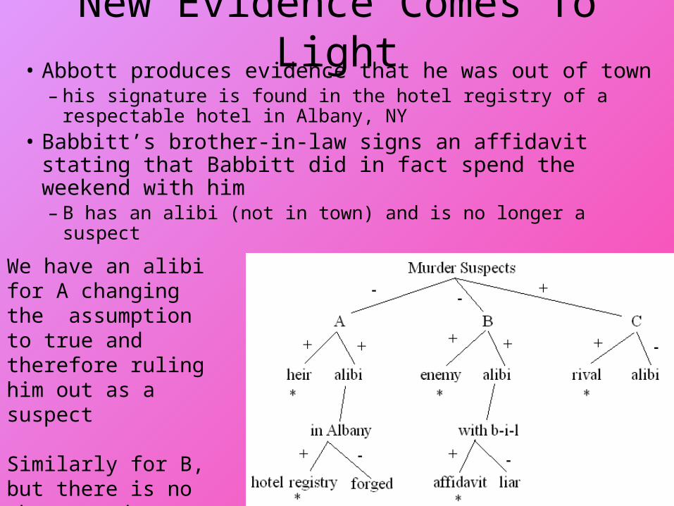
New Evidence Comes To Light• Abbott produces evidence that he was out of town
– his signature is found in the hotel registry of a respectable hotel in Albany, NY
• Babbitt’s brother-in-law signs an affidavit stating that Babbitt did in fact spend the weekend with him– B has an alibi (not in town) and is no longer a suspect
We have an alibi for A changing the assumption to true and therefore ruling him out as a suspect
Similarly for B, but there is no change made to C, so C remains a suspect

But Then…• B’s brother-in-law has a criminal record for perjury, so he is a
known liar– thus, B’s alibi is not valid and B again becomes a suspect
• A friend of C’s produces a photograph of C at the meet, shown with the winner– the photograph supports C’s claim that he was not in town and
therefore is a valid alibi, C is no longer a suspect
With these finalmodifications, B becomes our only suspect
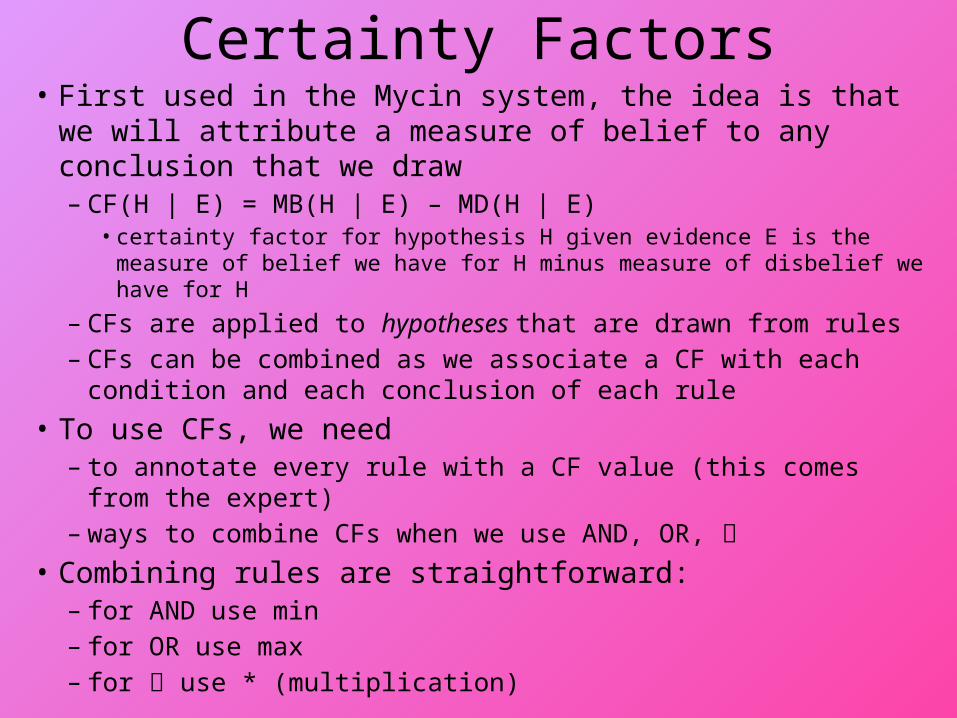
Certainty Factors• First used in the Mycin system, the idea is that we will
attribute a measure of belief to any conclusion that we draw– CF(H | E) = MB(H | E) – MD(H | E)
• certainty factor for hypothesis H given evidence E is the measure of belief we have for H minus measure of disbelief we have for H
– CFs are applied to hypotheses that are drawn from rules– CFs can be combined as we associate a CF with each condition
and each conclusion of each rule
• To use CFs, we need– to annotate every rule with a CF value (this comes from the expert)– ways to combine CFs when we use AND, OR,
• Combining rules are straightforward: – for AND use min– for OR use max– for use * (multiplication)
CF Example
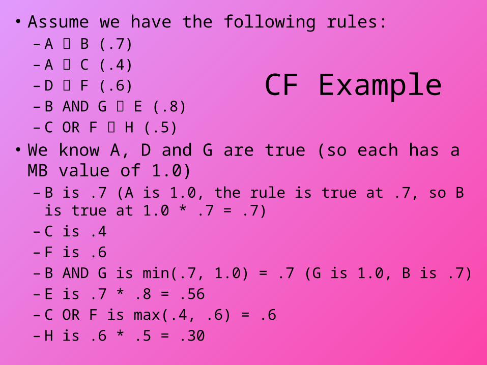
• Assume we have the following rules:– A B (.7)– A C (.4)– D F (.6)– B AND G E (.8)– C OR F H (.5)
• We know A, D and G are true (so each has a MB value of 1.0)– B is .7 (A is 1.0, the rule is true at .7, so B is true at 1.0 * .7 = .7)– C is .4– F is .6– B AND G is min(.7, 1.0) = .7 (G is 1.0, B is .7) – E is .7 * .8 = .56– C OR F is max(.4, .6) = .6– H is .6 * .5 = .30
Continued• Another combining rule is needed when we can
conclude the same hypothesis from two or more rules– we already used C OR F H (.5) to conclude H with a CF of
.30– let’s assume that we also have the rule E H (.5)– since E is .56, we have H at .56 * .5 = .28
• We now believe H at .30 and at .28, which is true?– the two rules both support H, so we want to draw a stronger
conclusion in H since we have two independent means of support for H
• We will use the formula CF1 + CF2 – CF1*CF2 – CF(H) = .30 + .28 - .30 * .28 = .496– our belief in H has been strengthened through two different
chains of logic

Fuzzy Logic• Prior to CFs, Zadeh introduced fuzzy logic to introduce
“shades of grey” into logic– other logics are two-valued, true or false only
• Here, any proposition can take on a value in the interval [0, 1]
• Being a logic, Zadeh introduced the algebra to support logical operators of AND, OR, NOT, – X AND Y = min(X, Y)– X OR Y = max(X, Y)– NOT X = (1 – X)– X Y = X * Y
• Where the values of X, Y are determined by where they fall in the interval [0, 1]

Fuzzy Set Theory• Fuzzy sets are to normal sets what fuzzy logic is to
logic– fuzzy set theory is based on fuzzy values from fuzzy logic
but includes set operations instead of logic operations
• The basis for fuzzy sets is defining a fuzzy membership function for a set– a fuzzy set is a set of items along with their membership
values in the set where the membership value defines how closely that item is to being in that set
• Example: the set tall might be denoted as – tall = { x | f(x) = 1.0 if x > 6’2”, .8 if x > 6’, .6 if x >
5’10”, .4 if x > 5’8”, .2 if x > 5’6”, 0 otherwise}– so we can say that a person is tall at .8 if they are 6’1” or we
can say that the set of tall people are {Anne/.2, Bill/1.0, Chuck/.6, Fred/.8, Sue/.6}

Hedges• Many use FL to represent English statements
– How do words like “very” or “somewhat” impact a membership function?
• for instance, we defined “Tall”, what does “Very tall” mean?
• These modifiers are implemented using hedge fuctions• A hedge for “very” might be to square the membership
value– If Chuck is tall with a membership of .6 then he is very tall
at a membership of .36– For “somewhat”, we might use square root so Chuck is
somewhat tall at sqrt(.6) = .77– Notice that Bill is all of “somewhat tall”, “tall” and “very
tall” at 1.0 so the hedges are not perfect
Fuzzy Membership Function
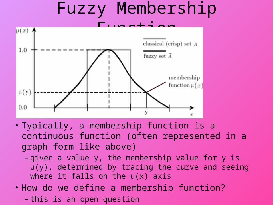
• Typically, a membership function is a continuous function (often represented in a graph form like above)– given a value y, the membership value for y is u(y),
determined by tracing the curve and seeing where it falls on the u(x) axis
• How do we define a membership function?– this is an open question

Using Fuzzy Logic/Sets• 1. fuzzify the input(s) using fuzzy membership functions• 2. apply fuzzy logic rules to draw conclusions
– we use the previous rules for AND, OR, NOT,
• 3. if conclusions are supported by multiple rules, combine the conclusions– like CF, we need a combining function, this may be done by
computing a “center of gravity” using calculus
• 4. defuzzify conclusions to get specific conclusions – defuzzification requires translating a numeric value into an
actionable item
• Fuzzy logic is often applied to domains where we can easily derive fuzzy membership functions and have a few rules but not a lot – fuzzy logic begins to break down when we have more than a
perhaps 10 rules
Example• Atmospheric controller increases or decreases temperature
and increases or decreases fan based on these rules– if air is warm and dry, decrease the fan and increase the coolant– if air is warm and not dry, increase the fan– if air is hot and dry, increase the fan and the increase the coolant
slightly– if air is hot and not dry, increase the fan and coolant– if air is cold, turn off the fan and decrease the coolant
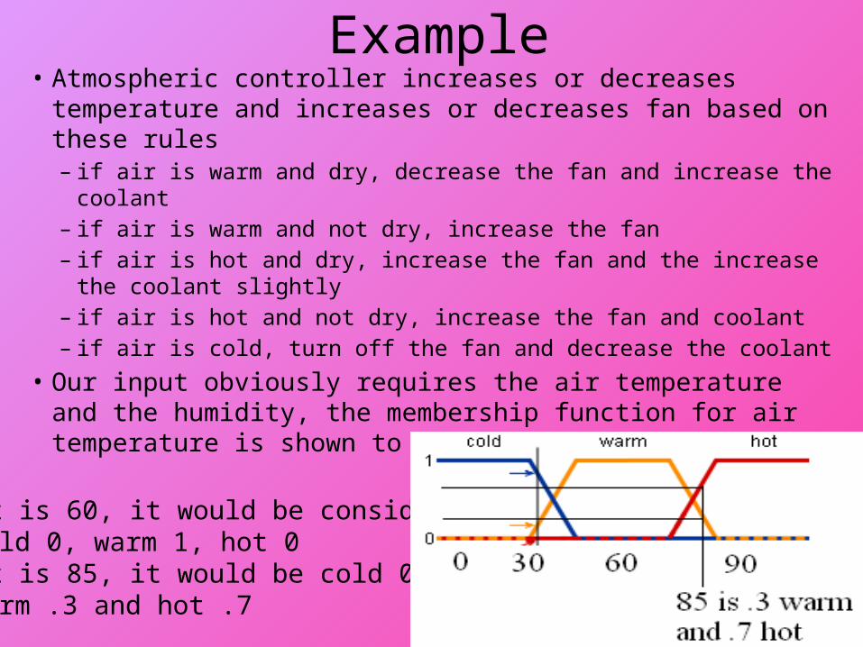
• Our input obviously requires the air temperature and the humidity, the membership function for air temperature is shown to the right
if it is 60, it would be considered cold 0, warm 1, hot 0
if it is 85, it would be cold 0, warm .3 and hot .7

Continued • Temperature = 85, humidity is moderately high
– hot .7, warm .3, cold 0, dry .6, not dry .4
• Rule 1 has “warm and dry”– warm is .3, dry is .6, so “warm and dry” = min(.3, .6) = .3
• Rule 2 has “warm and not dry”– min(.3, .4) = .3
• Rule 3 has “hot and dry” = min(.7, .3) = .3– our fourth and fifth rules give us 0 since cold is 0
• Our conclusions from the first three rules are to– decrease the coolant and increase the fan at levels of .3– increase the fan at level of .3– increase the fan at .3 and increase the coolant slightly
• To combine our results, we might increase the fan by .9 and decrease the coolant (assume “increase slightly” means increase by ¼) by .3 - .3/4 = .9/4
• Finally, we defuzzify “decrease by .9/4” and “increase by .9” to actionable amounts
Using Fuzzy Logic• The most common applications for fuzzy logic are for
controllers– devices that, based on input, make minor modifications to
their settings – for instance• air conditioner controller that uses the current temperature, the
desired temperature, and the number of open vents to determine how much to turn up or down the blower
• camera aperture control (up/down, focus, negate a shaky hand)• a subway car for braking and acceleration
• Fuzzy logic has been used for expert systems– but the systems tend to perform poorly when more than just a
few rules are chained together• in our previous example, we just had 5 stand-alone rules• when we chain rules, the fuzzy values are multiplied (e.g., .5 from
one rule * .3 from another rule * .4 from another rule, our result is .06)
Dempster-Shaefer Theory• The D-S Theory goes beyond CF and Fuzzy Logic by
providing us two values to indicate the utility of a hypothesis– belief – as before, like the CF or fuzzy membership value– plausibility – adds to our belief by determining if there is any
evidence (belief) for opposing the hypothesis
• We want to know if h is a reasonable hypothesis– we have evidence in favor of h giving us a belief of .7– we have no evidence against h, this would imply that the
plausibility is greater than the belief• p(h) = 1 – b(~h) = 1 (since we have no evidence against h, ~h = 0)
• Consider two hypotheses, h1 and h2 where we have no evidence in favor of either, so b(h1) = b(h2) = .5– we have evidence that suggests ~h2 is less believable than ~h1 so
that b(~h2) = .3 and b(~h1) = .5• h1 = [.5, .5] and h2 = [.5, .7] so h2 is more believable

Computing Multiple Beliefs• D-S theory gives us a way to compute the belief for any
number of subsets of the hypotheses, and modify the beliefs as new evidence is introduced– the formula to compute belief (given below) is a bit complex– so we present an example to better understand it– but the basic idea is this: we have a belief value for how well
some piece of evidence supports a group (subset) of hypotheses
• we introduce new evidence and multiply the belief from the earlier evidence with the belief in support of the new evidence for those hypotheses that are in the intersection of the two subsets
• the denominator is used to normalize the computed beliefs, and is 1 unless the intersection includes some null subsets
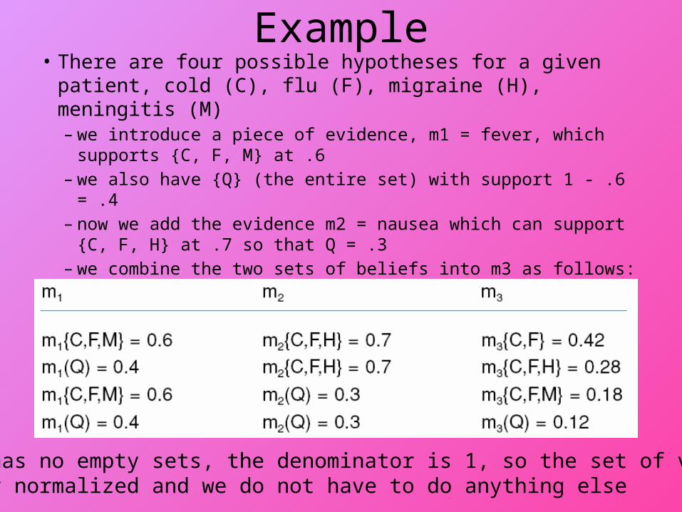
Example• There are four possible hypotheses for a given patient,
cold (C), flu (F), migraine (H), meningitis (M)– we introduce a piece of evidence, m1 = fever, which supports
{C, F, M} at .6– we also have {Q} (the entire set) with support 1 - .6 = .4– now we add the evidence m2 = nausea which can support {C,
F, H} at .7 so that Q = .3– we combine the two sets of beliefs into m3 as follows:
Since m3 has no empty sets, the denominator is 1, so the set of values in m3 is already normalized and we do not have to do anything else
Continued• When we had m1, we had two sets, {C, F, M} and {Q} • When we combined it with m2 (with two sets of its own,
{C, F, H} and {Q}), the result was four sets• the intersection of {C, F, M} and {C, F, H} = {C, F}• the intersection of {C, F, M} and {Q} = {C, F, M}• the intersection of {C, F, H} and {Q} = {C, F, H}• the intersection of {Q} and {Q} = {Q}
• We now add evidence m4 = lab culture result that suggest Meningitis, with belief = .8 – m4{M} = .8 and m4{Q} = .2
• In adding m4, with {M} and {Q}, we intersect these with the four intersected sets above which results in 8 sets – shown on the next slide, with some empty sets so our
denominator will no longer be 1 and we will have to compute it after computing the numerators
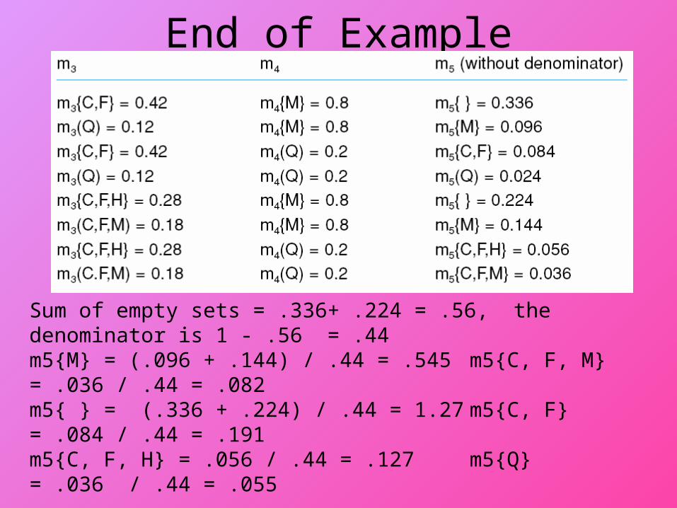
End of Example
Sum of empty sets = .336+ .224 = .56, the denominator is 1 - .56 = .44m5{M} = (.096 + .144) / .44 = .545 m5{C, F, M} = .036 / .44 = .082m5{ } = (.336 + .224) / .44 = 1.27 m5{C, F} = .084 / .44 = .191m5{C, F, H} = .056 / .44 = .127 m5{Q} = .036 / .44 = .055
The most plausible explanation is { } because the evidence tends to contradict (some symptoms indicate Meningitis, another symptom indicates no Meningitis), our best explanation otherwise is M at .545
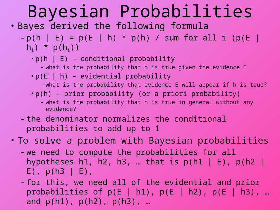
Bayesian Probabilities• Bayes derived the following formula
– p(h | E) = p(E | h) * p(h) / sum for all i (p(E | h i) * p(hi))• p(h | E) – conditional probability
– what is the probability that h is true given the evidence E
• p(E | h) – evidential probability– what is the probability that evidence E will appear if h is true?
• p(h) – prior probability (or a priori probability)– what is the probability that h is true in general without any evidence?
– the denominator normalizes the conditional probabilities to add up to 1
• To solve a problem with Bayesian probabilities– we need to compute the probabilities for all hypotheses h1,
h2, h3, … that is p(h1 | E), p(h2 | E), p(h3 | E), – for this, we need all of the evidential and prior probabilities
of p(E | h1), p(E | h2), p(E | h3), … and p(h1), p(h2), p(h3), …
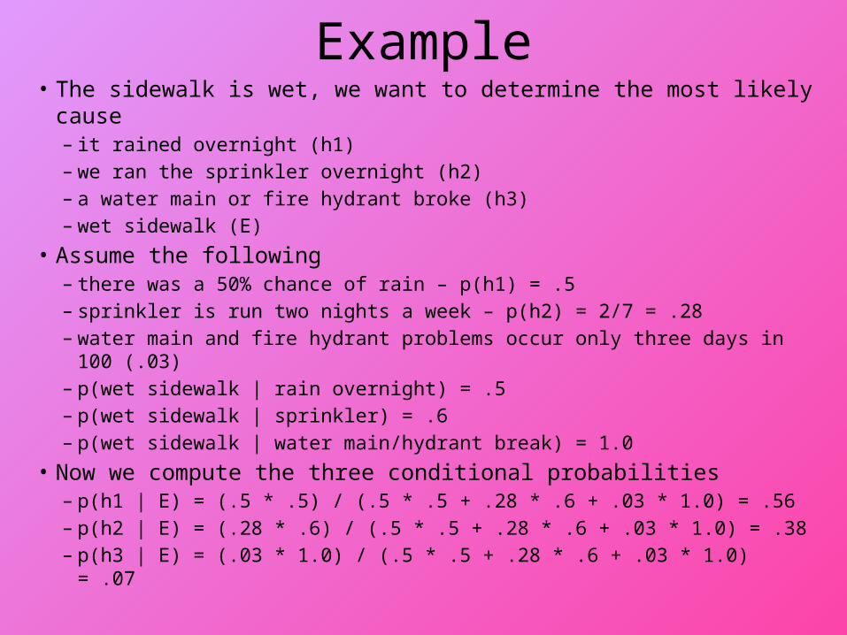
Example• The sidewalk is wet, we want to determine the most likely cause
– it rained overnight (h1) – we ran the sprinkler overnight (h2)– a water main or fire hydrant broke (h3)– wet sidewalk (E)
• Assume the following– there was a 50% chance of rain – p(h1) = .5– sprinkler is run two nights a week – p(h2) = 2/7 = .28– water main and fire hydrant problems occur only three days in 100 (.03)– p(wet sidewalk | rain overnight) = .5– p(wet sidewalk | sprinkler) = .6– p(wet sidewalk | water main/hydrant break) = 1.0
• Now we compute the three conditional probabilities– p(h1 | E) = (.5 * .5) / (.5 * .5 + .28 * .6 + .03 * 1.0) = .56– p(h2 | E) = (.28 * .6) / (.5 * .5 + .28 * .6 + .03 * 1.0) = .38– p(h3 | E) = (.03 * 1.0) / (.5 * .5 + .28 * .6 + .03 * 1.0) = .07

Independent Events• There is a flaw with our previous example
– if it is likely that it will rain, we will probably not run the sprinkler even if it is the night we usually run it, and if it does not rain, we will probably be more likely to run the sprinkler the next night
– also, if a water main or fire hydrant breaks, we will probably not have water to run the sprinkler
– therefore, our three causes are not independent of each other
• If we have dependencies, we cannot compute p(h | E) as simply– two events are independent if P(A, B) = P(A) * P(B) – when P(B) <> 0, then P(A) = P(A | B)
• that is, the P(A) is not impacted by B (whether B is true or false)
• Now we need further probabilities of p(h1, h2), p(h1, h3), p(h2, h3) and p(h1, h2, h3)

The Chain Rule• What is P(a, b, c, d)?
– More specifically, P(a=x1,b=x2,c=x3,d=x4)• these values are usually true or false although not always, especially if
any are input values and not hypotheses
• How do we compute this? Using the chain rule– p(a, b, c, d) = p(a) * p(b | a) * p(c | a, b) * p(d | a, b, c)– probabilities p(a) and p(b | a) are simple probabilities but p(c |
a, b) will is actually 4 probabilities (p(c | a=true,b=true), p(c | a=true,b=false), etc) and p(d | a, b, c) is 8 probabilities
• These more complex terms require an exponential number of probabilities because of dependencies– we have gone from needing n prior probabilities and n * m
evidential probabilities (given n causes and m pieces of evidence)
– to 2n prior probabilities and n*2m evidential probabilities
Naïve Bayes• We can apply Bayes in a naïve way meaning that
we assume independence of all evidence and hypotheses– This will not usually be true but it can still work well
when applied in some problems
• Consider a spam filter– We want to decide whether a given message is spam
or not– We want to build a classifier which rules yes or no
based on the conditional probability, that is • p(spam | email message)
– How do we compute this?

Spam Filter• First, we take a collection of email messages which include
spam– p(spam) = # spam messages / total– p(not spam) = # non spam messages / total
• We then collect all of the words of every spam message (we can throw out unimportant words like “a”, “and”, “the”, etc)– For a word, wi
• p(wi | spam) = number of spam messages in which wi appears
• p(wi | not spam) = number of non spam messages in which wi appears
– Given a new email message with words W = {w1, w2, w3, …, wn} compute
• p(spam | W) = p(spam) * p(w1 | spam) * p(w2 | spam) * … * p(wn | spam)
• P(not spam | W) = p(not spam) * p(w1 | not spam) * p(w2 | not spam) * … * p(wn | not spam)
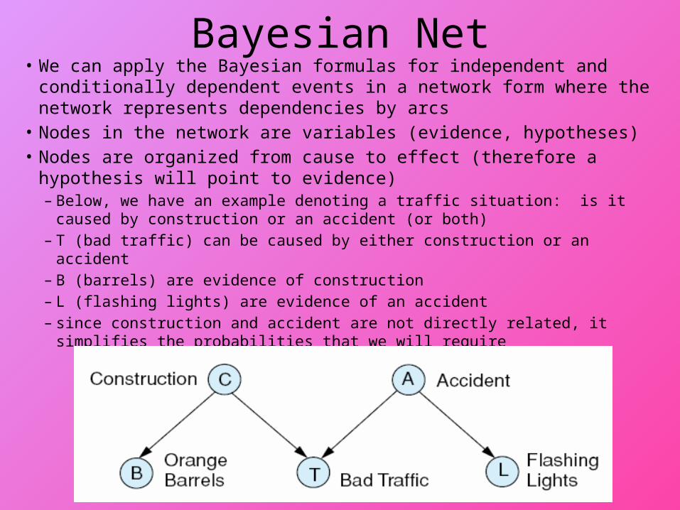
Bayesian Net• We can apply the Bayesian formulas for independent and conditionally
dependent events in a network form where the network represents dependencies by arcs
• Nodes in the network are variables (evidence, hypotheses)• Nodes are organized from cause to effect (therefore a hypothesis will point
to evidence)– Below, we have an example denoting a traffic situation: is it caused by
construction or an accident (or both)– T (bad traffic) can be caused by either construction or an accident– B (barrels) are evidence of construction – L (flashing lights) are evidence of an accident– since construction and accident are not directly related, it simplifies the
probabilities that we will require
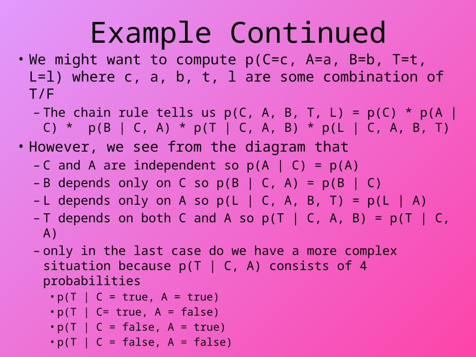
Example Continued• We might want to compute p(C=c, A=a, B=b, T=t, L=l)
where c, a, b, t, l are some combination of T/F– The chain rule tells us p(C, A, B, T, L) = p(C) * p(A | C) * p(B |
C, A) * p(T | C, A, B) * p(L | C, A, B, T)
• However, we see from the diagram that – C and A are independent so p(A | C) = p(A)– B depends only on C so p(B | C, A) = p(B | C)– L depends only on A so p(L | C, A, B, T) = p(L | A)– T depends on both C and A so p(T | C, A, B) = p(T | C, A)– only in the last case do we have a more complex situation because
p(T | C, A) consists of 4 probabilities• p(T | C = true, A = true)• p(T | C= true, A = false)• p(T | C = false, A = true)• p(T | C = false, A = false)
Another Example• We have a burglary alarm system which will
go off during a burglary but also sometimes during minor earthquakes
• Two neighbors of our house are John and Mary– John always calls when he hears the alarm but he
sometimes confuses the telephone with the alarm and calls mistakenly
– Mary sometimes misses the alarm
• We want to create a Bayesian network to model this and determine in different circumstances if there is a burglary or not
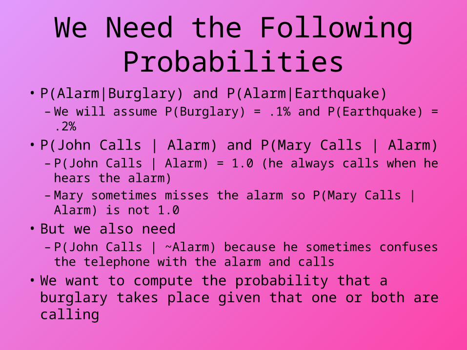
We Need the Following Probabilities
• P(Alarm|Burglary) and P(Alarm|Earthquake)– We will assume P(Burglary) = .1% and P(Earthquake) = .2%
• P(John Calls | Alarm) and P(Mary Calls | Alarm) – P(John Calls | Alarm) = 1.0 (he always calls when he hears
the alarm)– Mary sometimes misses the alarm so P(Mary Calls | Alarm) is
not 1.0
• But we also need– P(John Calls | ~Alarm) because he sometimes confuses the
telephone with the alarm and calls
• We want to compute the probability that a burglary takes place given that one or both are calling

Our Bayesian Network and Probs
burglary earthquake
Mary callsJohn calls
alarm
B E P(Alarm|B, E)T F
T T 0.95 0.05
T F 0.94 0.06
F T 0.29 0.71
F F 0.001 0.999
0.001
P(B)0.002
P(E)
0.95
0.94
0.29
0.001
T T
T F
F T
F F
P(A)B E
0.90
0.05
T
F
P(A)A
0.70
0.01
T
F
P(A)A
Probability alarm sounded but neither burglary nor earthquake has occurred and both John and Mary call is P(J ^ M ^ A ^ ~B ^ ~E) =
P(J | A) * P(M | A) *P(A | ~B ^ ~E) * P(~B) *P(~E) = 0.9 * 0.7 * 0.001 * 0.999* 0.998 = 0.00062
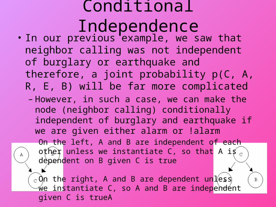
Conditional Independence• In our previous example, we saw that neighbor
calling was not independent of burglary or earthquake and therefore, a joint probability p(C, A, R, E, B) will be far more complicated– However, in such a case, we can make the node
(neighbor calling) conditionally independent of burglary and earthquake if we are given either alarm or !alarm
On the left, A and B are independent of each other unless we instantiate C, so that A is dependent on B given C is true
On the right, A and B are dependent unlesswe instantiate C, so A and B are independent given C is trueA

Example• Here, age and gender are independent
and smoking and exposure to toxins are independent if we are given age
• Next, smoking is dependent on both age and gender and cancer is dependent on both exposure and smoking and there’s nothing we can do about that
• But, serum calcium and lung tumor are independent given cancer
• So, given age and cancer– p(A, G, E, S, C, L, SC) = p(A) * p(G) *
p(E | A) * p(S | A, G) * p(C | E, S) * p(SC | C) * p(L | C)
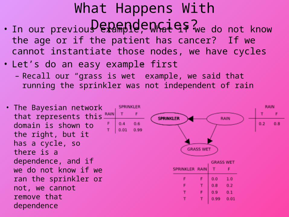
What Happens With Dependencies?• In our previous example, what if we do not know the age or
if the patient has cancer? If we cannot instantiate those nodes, we have cycles
• Let’s do an easy example first– Recall our “grass is wet” example, we said that running the
sprinkler was not independent of rain• The Bayesian network
that represents this domain is shown to the right, but it has a cycle, so there is a dependence, and if we do not know if we ran the sprinkler or not, we cannot remove that dependence

Solution• We must find some way of removing the cycle from the
previous graph– We will take one of the nodes that is causing the cycle and
instantiate it to true to compute our probability and then instantiate it to false and again compute our probability
– Our resulting probability will be the sum of the two
• Let’s compute p(rain | grass is wet) so that we will instantiate sprinkler to both true and false– p(rain | grass wet) = [p(r, g, s) + p(r, g, !s)] / [p(r, g, s) + p(r, g,
!s) + p(!r, g, s) + p(!r, g, !s)] = (.2 * .01 * .99 + .2 * .99 * .8) / (.2 * .01 * .99 + .2 * .99 * .8 + .8 * .4 * .9 + .8 * .6 * 0) = .36
– So there is a 36% chance that the grass is wet because it rained
• in the denominator, grass remains true throughout our denominator because we know that the grass was wet
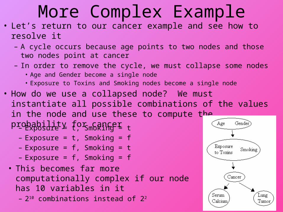
More Complex Example• Let’s return to our cancer example and see how to resolve it
– A cycle occurs because age points to two nodes and those two nodes point at cancer
– In order to remove the cycle, we must collapse some nodes• Age and Gender become a single node• Exposure to Toxins and Smoking nodes become a single node
• How do we use a collapsed node? We must instantiate all possible combinations of the values in the node and use these to compute the probability for cancer– Exposure = t, Smoking = t
– Exposure = t, Smoking = f– Exposure = f, Smoking = t– Exposure = f, Smoking = f
• This becomes far more computationally complex if our node has 10 variables in it – 210 combinations instead of 22
Junction Trees• With more forethought in our design
– we avoid collapsing nodes (requiring an exponential number of probabilities) by creating a junction tree (or join tree)
• The algorithm is roughly– start with an undirected graph version of our network– add additional arcs where we have independent nodes connected
to the same node (two or more parents connected to the same child) – these additional arcs are called “moral arcs”
– convert the graph to a triangulated graph by adding arcs such that every cycle of length >= 4 contains an edge connecting two non-adjacent nodes
– identify cliques in the triangulated graph• a clique is a set of nodes that is completely connected
– Create a new tree that consists of nodes representing each clique and join the cliques together by selecting setsets
• nodes which can connect separate clusters (cliques)
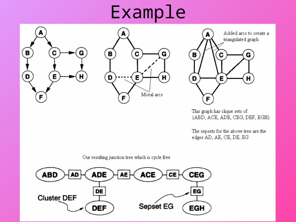
Example
Junction Trees• By adding the triangulated arcs, we wind up with
cliques of size 3– Thus, our junction tree consists of nodes that are of no
more than 3 combined (“joined”) nodes or variables• the number of probabilities we need for any given node is
no more than 8• with our previous approach to collapsing nodes, we would
require 2n probabilities where n was the number of nodes that required collapsing in order to remove the cycles
• so while the junction tree creation requires extra work, we save work in the long run by potentially greatly reducing the number of probabilities that we will have to deal with
Propagation• Recall earlier that if we did not know if it was raining in our
“grass wet” example, we would instantiate both raining is true and false– this can be computationally expensive especially if evidence is not
currently known but may become known later
• Judea Pearl came up with an approach for Bayesian nets that performs propagation of beliefs by making forward and backward passes across the network every time a new piece of evidence is received– we apply a bi-directional propagation algorithm rather than the
chain rule
• After we convert our belief net into a junction tree, we first perform processing within given nodes and then propagate those beliefs to neighboring nodes to create a “consistent” junction tree– we then normalize all probabilities to add up to 1

Propagation Algorithm• Initialize evidence as follows
– All evidence known to be true is set to 1 and false to 0– All evidence known with some belief is set to that belief (e.g., 0.8,
0.25)– All unknown evidence is set to 1
• Compute a node’s “potential”– Compute the probability for all possible values of the given variables –
plugging in any evidence that we know and using the prior and conditional probabilities when evidence is not known
• Perform global propagation as follows– Choose a node in the junction tree (randomly) and propagate outward
from that node to neighboring nodes recursively and once end nodes have been reached, propagate back inward
• Compute each variable’s probability by combining its computed probabilities in each node of the junction tree that contains it and then normalize all probabilities
Continued• We will skip the detail on the propagation algorithm as
it is very complex, references to study it are given online
• What if new evidence comes to light?– New evidence can be in one of three forms
• a previous unknown is now known to be true• a previous unknown is now known to be false• a previous known item’s status has changed (what was thought to
be true is now false or what was thought to be false is now true)
• We must re-propagate our beliefs– for the first case, we update the node(s) impacted by the
change in variable and propagate inward only– for the second and third cases, we update the node(s)
impacted by the change in variable and then perform the entire propagation (outward and inward)
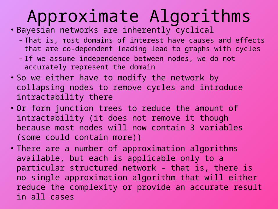
Approximate Algorithms• Bayesian networks are inherently cyclical
– That is, most domains of interest have causes and effects that are co-dependent leading lead to graphs with cycles
– If we assume independence between nodes, we do not accurately represent the domain
• So we either have to modify the network by collapsing nodes to remove cycles and introduce intractability there
• Or form junction trees to reduce the amount of intractability (it does not remove it though because most nodes will now contain 3 variables (some could contain more))
• There are a number of approximation algorithms available, but each is applicable only to a particular structured network – that is, there is no single approximation algorithm that will either reduce the complexity or provide an accurate result in all cases
Markov Models• Like the Bayesian network, a Markov model is a graph
composed of – states that represent the state of a process– edges that indicate how to move from one state to another
where edge is annotated with a probability indicating the likelihood of taking that transition
• An ordinary Markov model contains states that are observable so that the transition probabilities are the only mechanism that determines the state transitions– a hidden Markov model (HMM) is a Markov model where
the probabilities are actually probabilistic functions that are based in part on the current state, which is hidden (unknown or unobservable)
• determining which transition to take will require additional knowledge than merely the state transition probabilities
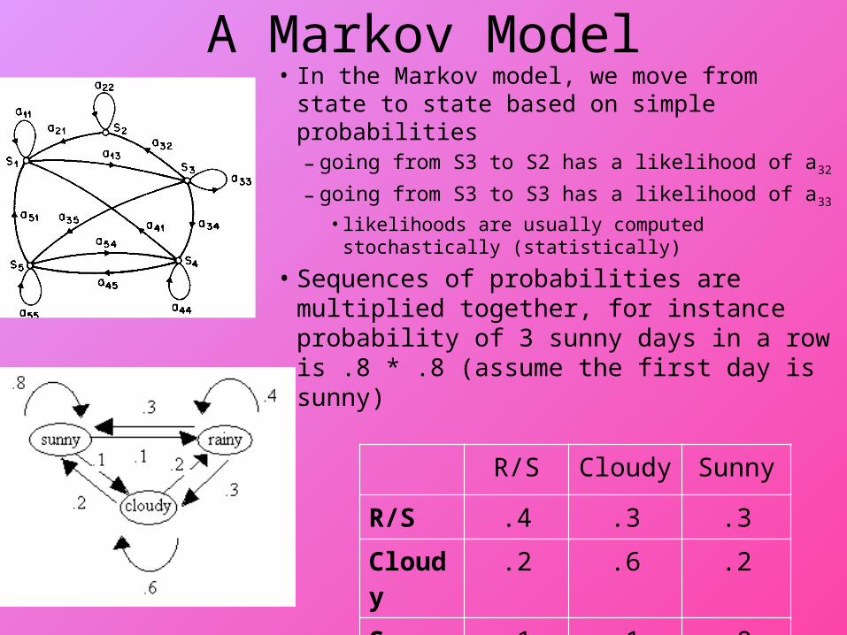
A Markov Model• In the Markov model, we move from state
to state based on simple probabilities– going from S3 to S2 has a likelihood of a32
– going from S3 to S3 has a likelihood of a33
• likelihoods are usually computed stochastically (statistically)
• Sequences of probabilities are multiplied together, for instance probability of 3 sunny days in a row is .8 * .8 (assume the first day is sunny)
R/S Cloudy Sunny
R/S .4 .3 .3
Cloudy .2 .6 .2
Sunny .1 .1 .8
HMM• Most problems cannot be solved by a Markov model
because there are unknown states– For instance, if we want to build an HMM for diagnosis,
we can view the symptoms while the diseases (hypotheses that describe what is wrong) are hidden
– The Markov model uses 2 probabilities: the prior probability of a node being true and the transition probability of moving from one node to another
– The HMM includes a third probability, the probability that being at a certain node (a visible state), a given hidden state is true
– As you will see in the next slide, the “visible states” are not actually part of the HMM’s nodes but instead denoted as additional probabilities (the b probabilities in the slide)
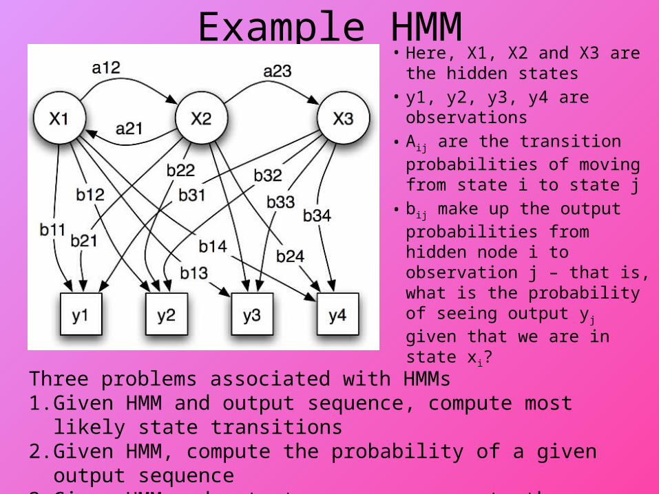
Example HMM• Here, X1, X2 and X3 are the
hidden states• y1, y2, y3, y4 are
observations
• Aij are the transition probabilities of moving from state i to state j
• bij make up the output probabilities from hidden node i to observation j – that is, what is the probability of seeing output yj given that we are in state xi?Three problems associated with HMMs
1. Given HMM and output sequence, compute most likely state transitions 2. Given HMM, compute the probability of a given output sequence3. Given HMM and output sequence, compute the transition probabilitiesSee the notes for more details
Where Do Uncertainty Values Come From?
• In all of the previous approaches (aside from non-monotonic reasoning), we need some specification of uncertainty– Certainty factors are provided by experts– Fuzzy membership values come from a fuzzy membership
function– Probabilities come from statistics
• CFs are based on the judgment of the expert– But the expert may not give consistent or reasonable values
• Fuzzy membership functions are made up!• Should we rely on statistics?
– Consider if we accumulate data for p(sneezing | flu) and p(flu) during the summer instead of the winter
Using Qualitative Uncertainty Values• If we want to use a rule-based approach, we do
not need specific numbers but instead relative statements of uncertainty– very likely, likely, somewhat likely, neutral, somewhat
unlikely, unlikely, very unlikely• experts often feel more comfortable with such terms
• Now we need some combining function– If one rule tells us flu is somewhat likely and another
rule tells us flu is likely, what is the resulting confidence in flu?
• Numeric scores are easy to come by but do not reflect human-level reasoning (usually)

Examples“Missing Else” syntax errorFeature 1: Is the prior statement an If-Then?Feature 2: Is there an "Else" statement in the prior statement?Feature 3: Is there a "Begin" immediately prior to the point of syntax error?Feature 4: Is there a missing "End" statement? Pattern 1: No ? ? ? = Ruled OutPattern 2: ? Yes ? ? = Somewhat UnlikelyPattern 3: ? ? ? Yes = Somewhat UnlikelyPattern 4: Yes No Yes No = Very LikelyPattern 5: Yes ? ? ? = Somewhat LikelyOtherwise Return Unlikely
“F” Recognizer
Feature 1: Line Vertical, Top Left, Medium Feature 2: Line Vertical, Middle Left, Medium Feature 3: Line Horizontal, Top Left, Small Feature 4: Line Horizontal, Middle Left, Small Feature 5: Line Horizontal, Bottom Left, Medium Feature 6: Line or Curve Right
Pattern 1: T T T T F F = Very LikelyPattern 2: T T T T ? ? = Somewhat LikelyPattern 3: T T T T F F (4) = Somewhat LikelyPattern 4: T T T T F F (3) = NeutralPattern 5: ? ? F F ? ? = Ruled OutOtherwise Return Very Unlikely
Other Mechanisms for Uncertainty• The artificial neural network (ANN) is an umbrella term that
describes a distributed representation for a set of knowledge– Within the representation, the ability to solve problems
(optimization, recognition, etc) is encapsulated as edge weights connecting “neurons”
– These edge weights are trained so that we do not have to supply them with values that may or may not be accurate
– The edge weights are real numbers and the nodes compute, using an activation function, whether they should be “on” or “off”, producing again real numbers
– So the ANN is a means of encapsulating uncertain knowledge and reasoning with uncertainty
– As the ANN is a form of machine learning, we cover the details in a couple of weeks
Continued• Another form of classifier is the support vector
machine– Consider that data that describe an entity will be
mapped into some n-dimensional Euclidean space– We want an SVM to determine a hyperplane that
separates data that are in the category from those that are not
– In order to determine the hyperplane, we train the SVM using one of several functions that attempt to derive the optimal hyperplane
– The result is an equation that, when a new test case is plugged in, determines whether the data describe an entity that is in or not in the class, computed as a real numbered value and thus with a degree of uncertainty