cardiovascular disease—risk benefits of clean fuel technology and policy: a statistical analysis

ARTICLE IN PRESS

Energy Policy 38 (2010) 1210–1222

Contents lists available at ScienceDirect

Energy Policy

0301-42

doi:10.1

n Corr

E-m

journal homepage: www.elsevier.com/locate/enpol

Cardiovascular disease—risk benefits of clean fuel technology and policy:A statistical analysis

Paul Gallagher a,n, William Lazarus b, Hosein Shapouri c, Roger Conway c,Fantu Bachewe b, Amelia Fischer a

a Economics Department, 481 Heady Hall, Iowa State University, Ames Iowa 50011, USAb Applied Economics Department, 253 COB, University of Minnesota, St. Paul, MN 55455, USAc Office of Energy Policy & New Uses, 400 Independence Avenue, SW (Rm.4059 So. Bldg), United States Department of Agriculture, Washington, DC 20250, USA

a r t i c l e i n f o

Article history:

Received 14 August 2009

Accepted 4 November 2009Available online 5 December 2009

Keywords:

Clean fuel regulation and technology

Health benefits

Biofuels

15/$ - see front matter & 2009 Elsevier Ltd. A

016/j.enpol.2009.11.013

esponding author. Tel.: +1 515 294 6181; fax

ail address: [email protected] (P. Gallagher).

a b s t r a c t

The hypothesis of this study is that there is a statistical relationship between the cardiovascular disease

mortality rate and the intensity of fuel consumption (measured in gallons/square mile) at a particular

location. We estimate cross-sectional regressions of the mortality rate due to cardiovascular disease

against the intensity of fuel consumption using local data for the entire US, before the US Clean Air Act

(CAA) in 1974 and after the most recent policy revisions in 2004. The cardiovascular disease rate

improvement estimate suggests that up to 60 cardiovascular disease deaths per 100,000 residents are

avoided in the largest urban areas with highest fuel consumption per square mile. In New York City, for

instance, the mortality reduction may be worth about $30.3 billion annually. Across the US, the

estimated Value of Statistical Life (VSL) benefit is $202.7 billion annually. There are likely three

inseparable reasons that contributed importantly to this welfare improvement. First, the CAA

regulations banned leaded gasoline, and mandated reduction in specific chemicals and smog

components. Second, technologies such as the Catalytic Converter (CC) for the automobile and the

low particulate diesel engine were adopted. Third, biofuels have had important roles, making the

adoption of clean air technology possible and substituting for high emission fuels.

& 2009 Elsevier Ltd. All rights reserved.

1. Introduction

Measurements of the health consequences of urban fuelconsumption are central to evaluation of regulations, technologiesand clean fuels that improve urban air quality. Presently,measurements combine known health effects with simulationsof emissions, ambient air quality, and mortality risk estimates(U.S. Environmental Protection Agency (2007); European Com-mission). However, estimated health effects emphasize short-runresponse to specific atmospheric chemicals. Further, the incor-poration of long-term effects of chronic and low level exposure toair pollution is incomplete. Long term effects of pollution onhealth are difficult to measure because the low level and chronicexposure must take place for several years before effects willoccur. Further, potential long-term effects are easy for critics todiscredit (Kittman).

Our estimate of the relation between an important healthindicator, the mortality rate for heart disease and stroke (HDS),and a pollution variable, the intensity of fuel consumption at a

ll rights reserved.

: +1 515 294 0221.

particular location, provides a glimpse of the overall long-termeffects of chronic exposure to air pollution. Optimistically,scientists will eventually understand the complex chemistry ofpollutant emission and transformation in the environment, andthe medical risks of chronic exposure to an array of urban aircomponents. Until then, reduced form equations can estimate thecomposite relation between the final (endogenous) effects andinitial (exogenous) causes (Greene, 2003, p. 379). Reduced formestimates can supplement an exhaustive understanding ofindividual cause and effect relationships. Specifically, we estimatethe total physical and social response to the technology improve-ments, product bans/substitutions, and economic policies asso-ciated with the US Clean Air Act (CAA) on HDS death risk—it isshown that the package of public actions had a substantialeconomic benefit.

Regarding organization, we first review the state of scientificunderstanding and uncertainty about air quality related determi-nants of health and HDS risk. Second, statistical estimates of thecross section relationship between the HDS mortality rate and theintensity of fuel consumption are presented. Third, policy-relatedreductions in HDS mortality are calculated by comparing slopes ofthe fuel intensity regression, before the US Clean Air Act (1974)and after the most recent policy revisions in 2004. Next, the

www.elsevier.com/locate/enpol

dx.doi.org/10.1016/j.enpol.2009.11.013

mailto:[email protected]

ARTICLE IN PRESS

P. Gallagher et al. / Energy Policy 38 (2010) 1210–1222 1211

cancer rate improvement estimate is combined with value ofstatistical life estimates (VSL) from the literature for a directstatistical estimate of overall program gains. Lastly, allocation ofthe overall welfare gain to components is discussed.

2. Fuel consumption-health relationships for policy analysis:state of knowledge and uncertainty

Exceptional complexity arises because the fuel consumption–human health relationship has at least three dimensions. First, theauto technology for burning fuel influences the composition andextent of chemical emissions into the atmosphere. And the nature ofemissions changes over time with changing auto technology andregulation. Second, the reactive chemicals emitted from vehicles aretransformed in the atmosphere, and sometimes the atmosphereitself is changed. Indeed, a separate branch of chemistry, atmo-spheric chemistry, has arisen in an attempt to understand theinteractions between fuel-based emissions and the air we breathe.Third, science understands that air pollution adversely influenceshuman health, but agreement on the mechanisms and effects isincomplete. The following statements illustrate that each of thecomponents also have multiple dimensions:

Combustion emissions and their contribution to ambient parti-culate, semivolitile, and gaseous air pollutants all contain organiccompounds that induce toxicity, mutagenicity, genetic damage,oxidative damage, and inflammation (Lewtas, 2007, p. 27).

Most of the medical literature on health risks from urban airpollution used in policy analysis focuses on short-run effectscaused by specific chemicals uniquely present in urban areas. Forinstance, ozone’s role in death from asthma, bronchitis, andemphysema has been verified and suggested for incorporation infuture policy analysis (Bailar et al., 2008). Less extreme healthproblems from the same diseases are emphasized in existingbenefit cost studies, but such studies frequently include a longerlist of health reducing chemicals (sulfates, carbon monoxide,nitrogen oxides, sulfur dioxide, and lead). For example, see(U.S. EPA (2007), p. D-6).

Generally speaking, the long run health risks from air pollutionare difficult to measure, because the many health effects arepresent only decades after exposure and air pollution is difficult toisolate as the sole cause (Cohen, 2003, p. 1011). One importantdeterminant of long run HDS risk, particulate air pollution, hasbeen included as a criterion for designing appropriate policies formitigating air pollution for policy analysis (Pope et al., 2002).Another study, not incorporated in policy analyses, suggests long-run relations between HDS risk and high emissions of nitrogenoxide and sulphate—apparently accumulated lead exposure(measured by bone lead) aggravates susceptibility in exposureto ozone and sulfates (Park et al., 2008, p. 6). Further, currentresearch investigations focus on the HDS risks associated withother elements of urban air that come from the gasoline engine,especially Polycyclic Aromatic Hydrocarbons (PAH) (Lewtas, 2007,p. 95). Urban air chemical–HDS risk relationships are partiallyknown, partially unknown.

The long run (HDS death rate) effect of policy and inducedtechnology changes should also be taken into account, becausegovernment policies are part of the fuel-health matrix. CAAsaimed at cleaner emissions have directly regulated enginetechnology and fuel recipes for both gasoline and diesel engines.Indirectly, these policies have caused a substitution of pollutingsubstances in favour of relatively clean additives. And fuel reciperegulations of the last 15 years have restricted several other toxicchemicals.

To curb the gasoline engine’s pollution, the catalytic converter(CC) was introduced in 1973 to remove olefins (highly reactivecompounds that promote smog formation) from auto exhaust.Leaded gasoline was gradually banned at the same time because itdamaged new cars equipped with the CC . There was animmediate decline in the urban population’s lead blood level asthe lead ban progressed (Kitman, 2000, p. 37). Further, a safeminimum threshold for exposure to lead apparently does notexist (Navas-Acien et al., 2007). Hence, a reduction in the long-runHDS rate due to the lead ban is plausible.

Production of high-octane lead-substitute additives increasedsteadily with the introduction of the CC. The lead ban wascomplete in 1995 (U.S. Department of Energy, pp. 9 and 22).Initially, MTBE, benzene-rich reformate, and ethanol shared thenew additive market, because they all had octane-boostingproperties that were similar to lead. When the 1990 CAA tookeffect, though, benzene restrictions were included to addresscancer mortality risks; benzene in reformulated fuel was limitedto 2.0% (U.S. Department of Energy, pp. 9). Recently, the benzenecontent of gasoline was limited to 0.62% in all gasoline (OctaneWeek (2007a, b), p.1). Also, MTBE was banned in several statesand mostly removed from the national market in 2005 amidstconcerns for ground water pollution. Gradually, ethanol substi-tutes have been removed from the lead-substitute market. Ineffect, the CC and ethanol are complementary inputs, used in fixedproportions, and jointly responsible for extensive HDS ratereductions over the last 20 years.

Particulate regulations for diesel were introduced after the1990 CAA. New standards specified cleaner diesel engines—a newheavy truck emitted 0.751 g/hp h of particulates before regula-tion, and gradually reduced to 0.1 g/hp h for 1994 models(U.S. Environmental Protection Agency (1985), p. 10630). It takesa long time for actual particulate reductions, however, owing tothe long useful life of a diesel truck.

Esther fuels from soybean or rapeseed oil also reduceparticulate emissions. Experimental data suggest that 20%esther-blended diesel fuel only emits 85% of the particulates of#2 fuel oil (Manicom et al.). Some esther-blend tests have shownan increase in nitrous oxide emissions. However, adjusted enginesreduce all categories of pollutants in some tests (Goetz). Overall,improved diesel engines and esther fuel blends are substituteinputs for reducing particulate emissions.

Separately, the CAA regulations of 1990 and 2000 both specifiedreduction in smog-causing gasoline engine emissions that wereachieved by regulating fuel composition (Ragsdale, 1994). Reducedcriteria pollutant emissions include chemicals with known HDS-provoking characteristics: nitrogen oxides, ozone (Gryparis et al.,2004), and sulphur oxides (Sunyer et al., 2003). Further, there arepotential long term effects due to an interaction between previouslead exposure and current susceptibility to ozone exposure (Parket al., 2008). Finally, emerging research on the HDS risks associatedwith PAH’s, and the appearance of these chemicals with particulates,suggest a possible understatement of the importance of gasolineemissions and regulations.

3. Estimation procedures

A disease rate-fuel intensity relationship underlies our em-pirical analysis. In Fig. 1, the function fi has a positive slopebecause residents of highly populated areas are exposed tohigher concentrations of pollutants from fuel consumption thanresidents of small towns or rural areas. Further, fi is hypothesizedto be relatively flat (has a smaller slope) when strict fuel blendingregulations, clean fuels that exclude harmful substances, or modernclean-burning engines dominate the vehicle fleet. In contrast, fi is

ARTICLE IN PRESS

f72

f04

gasoline intensity in county i, gi (in gallons/square mile)

HD

S m

orta

lity

rate

, dr i

(in

deat

hs p

er 1

00,0

00 p

eopl

e)

Fig. 1. HDS mortality rate—fuel intensity relationship.

1 See Appendix A for further discussion.2 These states are i=al, ar, az, ca, co, ct, dc, de, fl, ga, ia, id, il, in, ks, la, ma, md,

me, mi, mn, mo, ms, nc, ne, nh, nj, nm, nv, ny, oh, ok, or, pa, ri, sc, tn, tx, ut, va,

wa, wi.

P. Gallagher et al. / Energy Policy 38 (2010) 1210–12221212

hypothesized to be steeper before regulation, because older carsemitted more harmful exhaust pollutants, and fuel blending wasnot regulated for health benefits. Other factors may shift theposition of fi over time; examples of time-shifting variables includeimproving health care and deteriorating health habits such asobesity, drinking, and smoking. Our estimation of health benefitsconsists of estimating fi before the Clean Air Act in 1972, and afterthe CAA in 2004. Then the ‘other health determining factors’ areadjusted to their 2004 values, and a before and after comparison ofmortality rates is calculated.

We used the ‘fixed time and group effects’ model for crosssection-time series estimation (Greene, 2003, p. 291). Accord-ingly, the mortality rate is the dependent variable, and theintensity of fuel use is one explanatory variable. Additionally, adummy variable for the observation’s state and year are alsoincluded to capture the effects of other health determiningvariables. The regression specification is:

drit ¼StatDtitþSiaiDsitþbtgiitþeit ð1Þ

drit is the ‘age-adjusted’ mortality rate due to cardiovascular disease,in deaths/100,000 people; giit the fuel (gasoline and diesel) useintensity, in gallons/mi2; Dtit is 1 for year t (1972, 2004), and 0otherwise; Dsit is 1 for state s (s=al, ar, etc.), and 0 otherwise; eit is arandom variable; at, ai, bi are parameters for estimation

Eq. (1) defines 2 cross-section regressions, defined by t=72 andt=04. Also, the index, i, refers to sub-state observations, mainlymetropolitan counties of the US.

Initially, we expected to include explicit other health-deter-mining factors as explanatory variables. Some state-level data oncigarette consumption, weight status, and health expenditureswas available for recent years, but not for the pre-CAA period of1972. Further, local data were unavailable for both healthvariables in all time periods. Hence, we proxied the state of healthhabits, and health care delivery at each time and location using the‘state’ and ‘time’ variables. The death rate – fuel intensity – binaryvariable approach to estimation is likely viable under mostcircumstances. First, bias in regression coefficients due to anomitted explanatory variable, such as health habits, does not occurwhen the independent variables are uncorrelated (Judge et al.,

1982, p. 597). There is no reason to expect typical health habits tovary systematically across low density and high density urbanareas. Thus, bias in b due to exclusion of cigarette consumption,using 2001 data, is not extensive—the 2004 correlation betweenfuel intensity and cigarette consumption was � .01. Similarly, thecorrelation between fuel intensity and the fraction overweightpopulation was moderate, at � .13. Second, policy inferences basedon changes in the slope of the fuel consumption-health relation-ship are likely valid even in the presence of higher correlationsbetween fuel intensity and other (omitted) health variables,provided that the correlation pattern among independentvariables is similar before and after the policy change.1

The dependent variable in Eq. (1) removes the effect ofchanging age distribution. We used the ‘age adjusted’ death ratedue to cardiovascular disease. The age adjusted death rate forn age groups is:

dt

NTt

¼Xn

i ¼ 1

dit

Nit

Ni0

NT0

where

dit deaths in age group i and year t

Nit population in age group i in year t

dt ¼Xn

i ¼ 1

dit total deaths across age groups in year t

NTt ¼

Xn

i ¼ 1

Nit total population across age groups in year t

Ni0 population in age group i in base year 0 ð2000Þ

NT0 total population in base year 0 ð2000Þ

Thus, the actual mortality rate within each age group in eachcounty is weighted by a fixed age distribution proportion for abase year period. The 2000 age distribution of US populationdefines the fixed age distribution weights (National Center forHealth Statistics, p. 479).

For national policy analysis, it is convenient that the standardizednational death rate becomes the actual death rate in the base year.That is, d0=NT

0 ¼Pn

i ¼ 1 di0=NT

0 because Nit ¼Ni

0. Similarly for localdata, the actual death rate is approximately equal to the standar-dized death rate when the area’s age distribution is approximatelyequal to the national age distribution in the base year. Then thenumber of deaths is approximately equal to the current populationtimes the age adjusted death rate for the base year.

Estimation was executed on two cross-sectional regressionsusing the seemingly unrelated regression (SUR) procedure fromThe Statistical Analysis System (SAS) software package. Eachequation had its own intercept term, which defined two at’s. Anexplicit dummy variable takes a unit value (Dsi=1) for each state.2

Further, a particular state coefficient is constrained to be the sameacross both cross sectional equations.

4. Data

Individual death records data were compiled for our statisticalanalysis. The adjusted mortality rate data were constructed fromindividual records kept by the Center for Disease Control andmade available by the National Center for Health Statistics(National Bureau of Economic Research). Individual records wereavailable for 215 counties that were classified as metropolitan in1972, which were all included in the analysis.

ARTICLE IN PRESS

Table 1SUR estimate of heart disease and stroke mortality function.

dit ¼ 272:023Dt72þ220:229Dt04

ð56:13Þ ð41:02Þ

þ78:753 Dalitþ36:809 Daritþ15:986 Dcat � 14:296 Dcoitþ70:350 Ddeitþ13:291 Dflitþ28:169 Dgait

ð5:64Þ ð1:58Þ ð2:43Þ ð�1:16Þ ð3:02Þ ð1:84Þ ð2:26Þ

þ31:369 Diaitþ50:164 Dilitþ50:594 Dinitþ50:473 Dkyitþ59:550 Dlaitþ19:317 Dmaþ34:860 Dmdit

ð1:34Þ ð5:69Þ ð4:12Þ ð3:00Þ ð4:85Þ ð2:09Þ ð3:10Þ

þ45:765 Dmiitþ41:299 Dmoitþ32:001 Dmsitþ41:096 Dncitþ12:721 Dnhitþ44:325 Dnjit � 29:269 Dnmit

ð4:70Þ ð2:96Þ ð1:37Þ ð3:68Þ ð0:76Þ ð5:82Þ ð�1:25Þ

þ42:656 Dnvþ33:175 Dnytþ50:868 Dohitþ61:357 Dokitþ49:975 Dpaitþ36:342 Driitþ49:837 Dscitþ59:516 Dtnit

ð2:53Þ ð4:04Þ ð6:00Þ ð3:65Þ ð6:77Þ ð1:56Þ ð4:05Þ ð4:85Þ

þ22:152 Dtxitþ55:157 Dvaitþ19:276 Dwaitþ0:007483 gi72 � 0:00418 gi04

ð2:93Þ ð3:96Þ ð1:72Þ ð3:42Þ ð�1:39Þ

(Rural states of reference)

(MT, ND, SD, VT, WV, WY)

States without statistically significant Dsi;

i=AZ, CT, DC, ID, KS, ME, NE, OR, UT, WI

States with statistically significant and positive Dsi;

i=AL, AR, CA, DE, FL, GA, IA, IL, IN, KY, LA, MA, MD, MI, MO, MS, NC, NH, NJ, NM, NY, OH, OK, PA, RI, SC, TN, TX, VA, WA

States with statistically significant and negative Dsi;

i=CO, NM

adj.R272=.3575

adj.R204=.1742


The gasoline intensity variable was also constructed. We usedcounty level data on Vehicle miles travelled (VMT), which iscollected jointly by the US Department of Transportation and theU.S. Environmental Protection Agency (Driver et al., 2007). The VMTdata was combined with fuel economy estimates for the appropriateyear from the EPA’s MOBILE6 model (e.g., Landman). Fuelconsumption for each county was approximated by multiplyingmiles by fuel economy, and aggregating across vehicle classes. Wematched 1978 VMT data with the pre-regulation cardiovasculardisease rate observation, because it was the earliest data available.Lastly, fuel consumption for each county or ‘other state’ observationwas divided by the geographical area of the appropriate unit.

Also, 48 ‘other state’ or ‘rural’ observations were used forpreliminary estimations. These observations were constructed bysubtracting the appropriate metropolitan counties from statelevel data.3,4 This extended the range of exposure on the low side,and increased the sample size to 263 observations in each year.

3 For the dependent variable, the raw data, the number of cardiovascular disease

deaths by age group, was given at the state level and for each metropolitan county.

The total number of deaths (by age group) for the rural ‘‘rest of state’’ region is the

residual difference between the number of deaths in the state less the sum of deaths

in the metro counties. The population data by age group is also given at the state and

metro-county level by age groups. So the residual population by age group in

the rural rest-of-state region is the state population less the sum of population in the

metro counties. Next, the death rate by age group for the rural was calculated as the

ratio of the number of deaths divided by the population for each age group.

Finally, the ‘‘age adjusted death rate’’ was calculated as a weighted average using

weights from the national average age distribution.

For the fuel intensity variable, we started with fuel consumption data at the state

level and for the metro-counties. So the ‘‘rural fuel consumption’’ was calculated as

the difference between state consumption and the sum of metro-county consump-

tion. Next, we obtained data on the physical area of each state and metro-counties.

Then we calculated the area of the rural area as the difference between the state total

and the sum of urban counties-area. Finally, fuel intensity for the rural area is rural

fuel consumption divided by rural population.4 The ‘other state’ observations do extend the physical area of some

observations, but not abruptly. Specifically, one-half of the ‘other state’ areas are

smaller than the largest county in the sample. Further, one-fourth of the other

state areas are no more than twice the size of the second largest county.

5. Estimates

Estimates for the mortality rate function were based on Eq. (1).But several specifications were estimated to evaluate inclusion ofspecific dummy variables. Preliminary estimates suggested thatboth time dummies were significant and should be included.Initially, the Dsi=0 situation refers to six rural states that did nothave a metropolitan county in the 1972 reference data (mt, nd, sd,vt wv, and wy). Other state dummies were also excluded whenthe effect was not significantly different from zero. Furthermore,including rural observations did not affect the estimates, andprecluded calculation of 2004 fuel-health correlations becauseappropriate state-level health data were unavailable. Hence, ruraldata is excluded from the reported results (Table 1).5

The estimated mortality response function is given in Table 1,and t-values for individual variables indicate statistically sig-nificant effects. The reported set of explanatory variables explainabout one-third of sample variation in the two sample years,which is typical for cross sectional regressions.

Regarding the magnitude of estimated coefficients, the twotime dummies suggest an increase in the mortality rate over time.Also, the state effects that are positive, zero, and negative definethree groups of states (which are summarized in Table 1). Thestate with the largest positive effect is Alabama, and the statewith the lowest negative effect is New Mexico. Time and spatialvariation in these effects can be attributed to changing health caretechnology, health care delivery, and health habits in particularlocations. Indeed, the pattern of state dummies with largenegative effects in several southern states conforms to prelimin-ary estimates for the 2004 regression with available cigaretteconsumption data for 2004—cardiovascular disease rates tendedto be high in the south (Alabama, Louisiana, Oklahoma, andVirginia).

5 Similar estimates that include these rural observations are given in

Appendix B.

ARTICLE IN PRESS

0

50

100

150

200

250

300

350

0

fuel use, in gallons / sq. mi

HD

S de

ath

rate

, in

deat

hs p

er 1

00,0

00

19722004

1000 2000 3000 4000 5000 6000

Fig. 2. Estimated death rate vs. fuel intensity: 2004 basis.


The estimated response to the fuel intensity variable isimportant for policy analysis. As anticipated, the slope effect forthe initial period is significant. Further, the fuel intensity for 2004effect is smaller and not statistically significant.6

One would not expect a negative estimate b04 in Table 1 whenall health shifting variables are uncorrelated with gi. In the strictlyurban sample defining the results of Table 1 and Appendix D,however, there is a moderate negative correlation betweenoverweight and fuel intensity in 2004. A priori bias analysissuggests that the estimate b04 would be low without theoverweight variable. The 2004 regression of an all urban samplewith the overweight variable included (in Appendix Table D1bears this out—here, b04 is positive but not strictly significant.

Still, the estimate of the difference, b04 � b72, drives the policyanalysis. The analysis of Appendix A suggests that unbiaseddifference estimates will likely occur. Unbiased differenceestimates should hold as long as the overweight/fuel intensityintercorrelation across counties holds in both time periods.Overall, the results of Table 1 (and Table B1) confirm that theimpact of increasing fuel intensity on HDS has been reduced sinceCAAs, CC, and ethanol. However, one should not necessarilyconclude that the effect is eliminated.

7 For demonstration, the mortality function estimate in the terminal period n

is:

din ¼ anDtnþ aiDsinþ bngin:

The mortality function estimate in the initial period 0 is:

di0 ¼ a0Dt0þ aiDsi0þb0gi0 :

So the pre-policy mortality function in today’s health situation is:

d�i0 ¼ anDtnþ aiDsinþ b0gi0 :

Taking the difference gives:

D¼ din � d�in ¼ bngin � b0gi0 :

Assuming that fuel intensity does not change, gin=gio=gi, gives:

D¼ ðbn � b0Þgi:

The statistic, approximation holds with our large sample. Hence, the null

hypothesis, no change in the mortality function associated with the policy, is

rejected at any reasonable significance level.

6. Calculations of policy change effects

We now present the mortality rate reduction and associatedeconomic value associated with the policy change, includingindividual metropolitan areas and for the entire US. First, thecalculation of mortality rate change is explained. Second, thevaluation procedure is discussed. Third, the calculations arepresented.

6.1. Mortality change

For an estimate of today’s cardiovascular disease risk withoutthe CAA policies, use today’s values for ‘other health variables’with the 1972 estimate of the mortality response to fuel intensity.Thus, the level and position of today’s response functions with theCAA and without the CAA are identified. These two responsecurves are shown in Fig. 2. The lower response curve is calculatedusing 2004 values of binary variables and the 2004 coefficient forfuel intensity. The upper response curve differs only in the use of

6 2004 regression that includes other health variables is given in Appendix

Table D1. The estimated fuel intensity effect for 2004 is not significant, but may

suggest that a positive effect remains.

the 1972 coefficient for fuel intensity response. The mortality gainfrom the CAA policies for a county with a given g is defined by thedifference between the two response curves.

Further, there is a statistically significant difference betweenthe post-policy and the pre-policy mortality rate function. Whenthe ‘pre-function’ and the ‘post-function’ are compared on a 2004basis with a given fuel intensity level, the statistic, t=D/sd(D),has a t distribution with N-K degrees of freedom under thenull hypothesis that the mortality function does not changewith CAA policy.7 For the estimates of Table 1, D=�0.011663,sd(D)=0.00357, and t=�3.25. Also, a normal approximation holdswith our large sample. Hence, the null hypothesis, no change inthe mortality function associated with the policy, is rejected atany reasonable significance level.

However, an ex post estimate of the mortality change frompolicy inception should probably take into account the change infuel intensity over the period, as well as the shift in the mortalityfunction. The estimate of mortality rate change in county i sincethe policy change is

Di ¼ b04gi04 � b72 gi72:

Or Di ¼ ðb04 � b72Þgi04þ b72 Dgi; where Dgi ¼ gi04 � gi72

Then the mortality change accross all counties is

D¼P

Di:

6.2. Valuation

We use a Value of Statistical Life (VSL) estimate to value themortality reduction associated with the CAAs. Now we summar-ize the important concepts, estimates and limitations associatedwith this method.

Measurements of individuals’ willingness to trade money for aslightly higher death risk often rely on a statistical relationshipbetween wages and the risk of accidental death in variousoccupations (Moore and Viscusi, 1988, p. 484). The essentialestimates from a well-known cross sectional study are

lnðwiÞ ¼ kþ0:0075 pi � 0:0081 pici;

t¼D=sdðDÞ ¼bn � boffiffiffiffiffiffiffiffiffiffiffiffiffiffiffiffiffiffiffiffiffiffiffiffiffiffiffiffiffiffiffiffiffiffiffiffiffiffiffiffiffiffiffiffiffiffiffiffiffiffiffiffiffiffiffiffiffiffiffiffiffiffiffiffiffiffiffiffiffiffiffiffi

VarðbnÞþVarðboÞ � 2Cov1ðbn; boÞ

q

has a t distribution with N-K degrees of freedom (Kmenta, p. 372).

ARTICLE IN PRESS

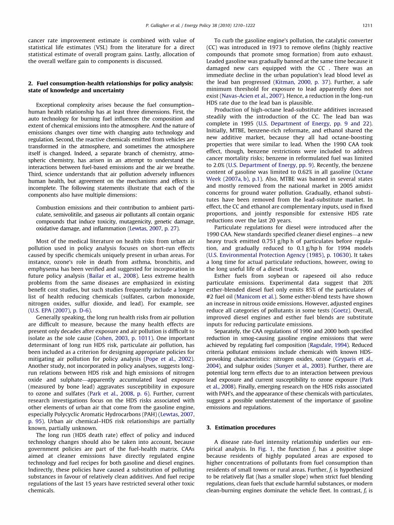
Table 2Mortality (heart disease and stroke) reductions and lives saved by clean air act: counties with largest effects, and total US.

State County seat 2004 Fuel use (gal/mi2) 2004 Population Mortality change

(deaths/100,000)

Deaths avoided:

Number Value-VSL (mil. $)

Most improvement in mortality—top 10 counties

DC DC 5148.1 554,239 �60.431 �335 2344.5

NY White Plains 3996.4 941,380 �55.617 �524 3664.9

PA Philadelphia 3875.4 1,471,255 �55.111 �811 5675.7

NY New York 3393.2 8,164,706 �53.095 �4335 30,345.5

NJ Jersey City 3342.1 605,359 �52.882 �320 2240.9

NJ Newark 3400.5 795,015 �51.165 �407 2847.4

PA Doylestown 3663.3 617,214 �50.471 �312 2180.6

MD Baltimore 3550.2 641,943 �45.575 �293 2047.9

NJ Elizabeth 3552.4 530,846 �41.736 �222 1550.9

MA Boston 2915.5 664,263 �39.919 �265 1856.2

Subtotal �7822 54,754.5

Most improvement in mortality—top 20 counties

MI Mount Clemens 3213.0 822,965 �38.514 �317 2218.7

NY Goshen 2277.0 369,511 �38.258 �141 989.6

PA Easton 2676.1 283,333 �37.745 �107 748.6

IL Decatur 5200.0 674,335 �36.421 �246 1719.2

CA Oakland 2800.2 1,452,096 �35.203 �511 3578.2

MI Detroit 2680.7 2,013,771 �32.812 �661 4625.4

NJ Boston 2915.5 664,263 �31.432 �283 1856.2

CO Denver 3173.7 555,991 �28.960 �161 1127.1

NY New City 3029.4 293,049 �28.819 �84 591.2

DE Wilmington 2579.4 518,728 �28.833 �150 1046.9

Subtotal �2661 18,501.1

Total, United States �28,915 202,999

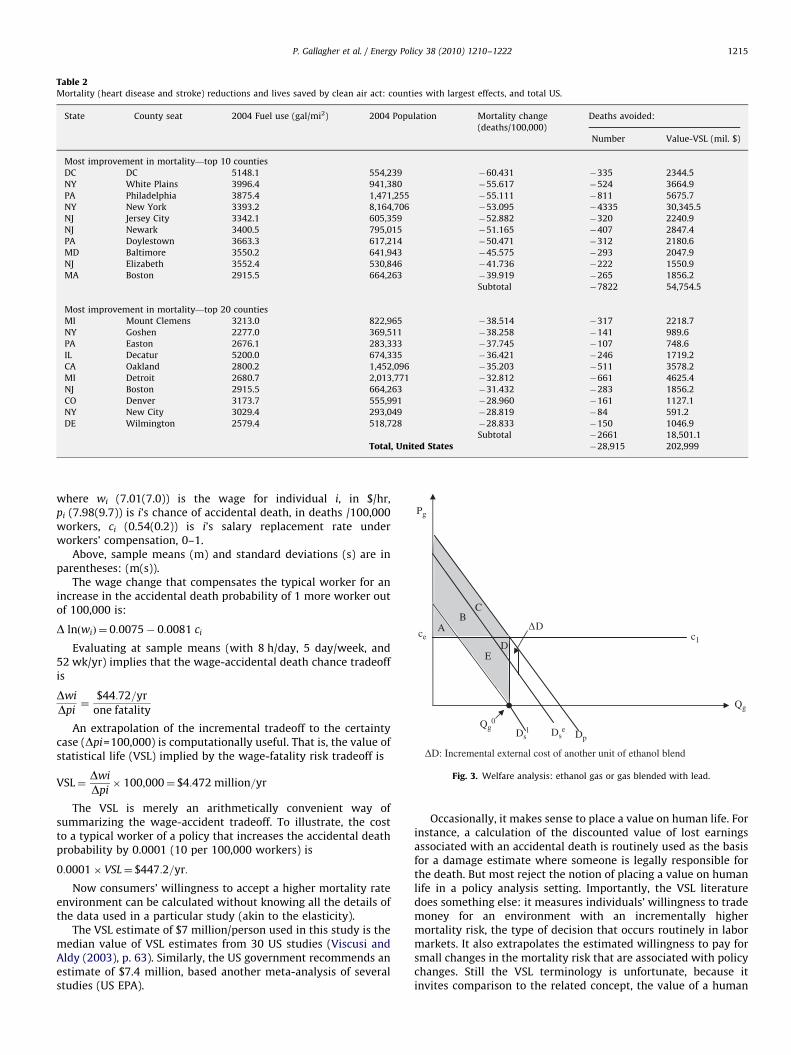
ΔD: Incremental external cost of another unit of ethanol blend

Qg

ΔD

Pg

ce

C

Qg0

Dsl Ds

eDp

c1

E

BA

D

Fig. 3. Welfare analysis: ethanol gas or gas blended with lead.


where wi (7.01(7.0)) is the wage for individual i, in $/hr,pi (7.98(9.7)) is i’s chance of accidental death, in deaths /100,000workers, ci (0.54(0.2)) is i’s salary replacement rate underworkers’ compensation, 0–1.

Above, sample means (m) and standard deviations (s) are inparentheses: (m(s)).

The wage change that compensates the typical worker for anincrease in the accidental death probability of 1 more worker outof 100,000 is:

D lnðwiÞ ¼ 0:0075� 0:0081 ci

Evaluating at sample means (with 8 h/day, 5 day/week, and52 wk/yr) implies that the wage-accidental death chance tradeoffis

Dwi

Dpi¼

$44:72=yr

one fatality

An extrapolation of the incremental tradeoff to the certaintycase (Dpi=100,000) is computationally useful. That is, the value ofstatistical life (VSL) implied by the wage-fatality risk tradeoff is

VSL¼Dwi

Dpi� 100;000¼ $4:472 million=yr

The VSL is merely an arithmetically convenient way ofsummarizing the wage-accident tradeoff. To illustrate, the costto a typical worker of a policy that increases the accidental deathprobability by 0.0001 (10 per 100,000 workers) is

0:0001� VSL¼ $447:2=yr:

Now consumers’ willingness to accept a higher mortality rateenvironment can be calculated without knowing all the details ofthe data used in a particular study (akin to the elasticity).

The VSL estimate of $7 million/person used in this study is themedian value of VSL estimates from 30 US studies (Viscusi andAldy (2003), p. 63). Similarly, the US government recommends anestimate of $7.4 million, based another meta-analysis of severalstudies (US EPA).

Occasionally, it makes sense to place a value on human life. Forinstance, a calculation of the discounted value of lost earningsassociated with an accidental death is routinely used as the basisfor a damage estimate where someone is legally responsible forthe death. But most reject the notion of placing a value on humanlife in a policy analysis setting. Importantly, the VSL literaturedoes something else: it measures individuals’ willingness to trademoney for an environment with an incrementally highermortality risk, the type of decision that occurs routinely in labormarkets. It also extrapolates the estimated willingness to pay forsmall changes in the mortality risk that are associated with policychanges. Still the VSL terminology is unfortunate, because itinvites comparison to the related concept, the value of a human

ARTICLE IN PRESS

Table B1SUR estimate of heart disease and stroke mortality function: rural counties are included.

dit ¼ 274:623 Dt72þ210:473 Dt04

ð70:85Þ ð48:78Þ

þ76:695 Dalitþ42:185 Daritþ17:515 Dcat � 21:969 Dcoitþ57:068 Ddeitþ12:053 Dflitþ32:818 Dgait

ð6:44Þ ð2:56Þ ð2:96Þ ð�2:04Þ ð3:47Þ ð1:84Þ ð3:02Þ

þ21:068 Diaitþ50:347 Dilitþ49:657 Dinitþ55:924 Dkyitþ60:891 Dlaitþ16:784 Dmaþ34:535 Dmditþ21:561 Dme


þ45:419 Dmiitþ41:298 Dmoitþ51:006 Dmsitþ43:354 Dncitþ15:215 Dnhitþ44:852 Dnjit � 27:655 Dnmit

ð5:16Þ ð3:47Þ ð3:10Þ ð4:37Þ ð1:12Þ ð6:41Þ ð�1:68Þ

þ28:358 Dnvþ34:793 Dnytþ51:743 Dohitþ58:854 Dokitþ51:789 Dpaitþ29:438 Driitþ53:508 Dscitþ61:510 Dtnit


þ24:209 Dtxitþ46:474 Dvaitþ16:352 Dwaitþ :00627 gi72þ :001142 gi04

ð3:53Þ ð3:91Þ ð1:65Þ ð3:05Þ ð0:41Þ

(Rural states of reference)

(MT, ND, SD, VT, WV, WY)


i=AZ, CT, DC, ID, KS, NE, OR, UT, WI


i=AL, AR, CA, DE, FL, GA, IA, IL, IN, KY, LA, MA, MD, ME, MI, MO, MS, NC, NH, NJ, NM, NY, OH, OK, PA, RI, SC, TN, TX, VA, WA


i=CO, NM

adj.R272=.3599

adj.R204=.2389


life, which is objectionable. Ironically, more obscure economiclanguage would probably enhance widespread understanding ofthe VSL concept.

VSL estimates have some characteristics that are consistentwith willingness to pay or accept concepts. First, VSL estimatesare higher in wealthy countries than in poor countries. This mayexplain why wealthier societies are more interested in environ-mental regulations that improve health. On the other hand, itwould likely preclude across country comparisons. Second, VSL iswill likely increase with an individual’s age due to the accumula-tion of wealth. In contrast, a discounted value of lost earningsestimate would decrease with age. In short, VSL will notdiscriminate against wealthy old people. But it might not assignan appropriate value for poor young people.

6.3. Results

The estimates of mortality reduction in Table 2 do account forthe change in the mortality function and the fuel intensity change.Then the death reduction is calculated as the mortality ratereduction times the 2004 population. In turn, the mortality ratereduction includes slope and fuel use changes. We estimate anannual death reduction of 7823 people annually for the highest 10cities, a cumulative total 10,589 people annually for the top 20cities, and 29,000 people for the entire US.8

For valuation, we estimate that the combined reductions,technology advances, and subsidies provide an annual value of$203 billion for the entire US. Further, the 10 high cities reducetheir annual loss by nearly $55 billion and the top 20 cities reducetheir death loss by $74.1 billion, annually. That is, the value ofreduced loss of human life is $203 billion throughout the US.

For comparison, the changing fuel intensity effect reduced theUS VSL estimate by about 8%, from $221 billion to the $203 billion

8 Estimates of mortality reduction from CAA policies for all counties, sub-state

rural areas, and the US are given in Appendix Table C.

shown in Table 2. There were a few large coastal cities withreduced fuel intensity between 1972 and 2004, possibly due tothe development of mass transit. Otherwise, fuel intensityincreased between 1972 and 2004 partially offsetting themortality function decline.

7. Welfare interpretation of estimates

To welfare economics, the $203 billion estimate of annualcardiovascular disease reduction benefit represents a marketexternality. Next we show how policy, technology, and productsubstitution reduced the size of the cardiovascular disease riskand internalized the externality. We also discuss effects of today’sincremental fuel changes with current CAA policy, technology,and substitution possibilities in place

To illustrate, consider the market for gasoline that is blendedwith high-octane gasoline additives. In Fig. 3, the private demandfor mixed gasoline is Dp. Initially, suppose the supply is defined byconstant-cost production of leaded-fuel, C1. In the initial baseline,the actual social demand curve, Ds

1, is below Dp due to the adversecardiovascular disease and other health effects of smog formed byusing the lead additive to produce blended gasoline. Next, a policychange jointly requires the catalytic converter (CC), bans lead, andintroduces ethanol. Then ethanol-blended gasoline’s socialdemand curve, Ds

e, is slightly below private demand, Dp. Forillustration, suppose that the ethanol blend has the sameproduction cost as lead: Cl=Ce. Then gasoline (blended fuel)output is the same, at Qg

0, initially, and after joint CC introduction,lead ban, and ethanol development.

Now consider the welfare change. Before the policy change,consumer surplus is A+B+C, external cost is B+C+D+E, and netsurplus level is A�(D+E). After the policy change, consumersurplus is still A+B+C. But external cost, C+D, is smaller.Consequently, net benefit level, A+B�D, is larger. Taking thedifference between the final and initial welfare areas gives the

ARTICLE IN PRESS

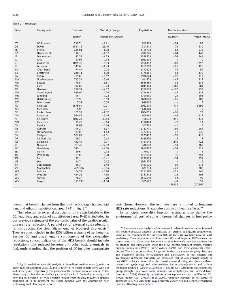
Table C1Mortality reductions and lives saved by clean air act, county by county.

State County seat Fuel use Mortality change Population Deaths Avoided

gal/mi2 Deaths per 100,000 Number Value (mil $)

AL Birmingham 639.5 �6.80 658468 �45 314

AL Huntsville 313.9 �3.20 293598 �9 66

AL Mobile 198.2 �2.35 400107 �9 66

AR Little rock 655.37 �5.29 365228 �19 135

AZ Phoenix 335.96 �2.45 3498587 �86 600

AZ Tuscon 76.9 �0.67 906540 �6 43

CA Oakland 2800.21 �35.20 1452096 �511 3578

CA Visalia 66.8 �0.78 400952 �3 22

CA Ventura 217.1 �2.21 796165 �18 123

CA Martinez 936.7 �8.89 1007606 �90 627

CA Fresno 109.4 �1.13 865620 �10 69

CA Bakersfield 471.63 �4.82 734077 �35 248

CA Los Angeles 1255 �13.33 9917331 �1322 9254

CA Salinas 98.2 �1.05 414551 �4 30

CA Santa ana 2136.9 �19.21 2982094 �573 4010

CA Riverside 1631.97 �14.37 1869465 �269 1880

CA Sacremento 965.2 �8.58 1351428 �116 812

CA San bernardino 752.56 �7.87 1916418 �151 1056

CA San diego 536.9 �4.84 2935190 �142 995

CA San fransisco 1744 �24.62 743193 �183 1281

CA Stockton 1108.32 �13.70 649241 �89 623

CA Redwood city 897.5 �8.65 698156 �60 423

CA Santa barbara 76.5 �0.77 401708 �3 22

CA San jose 958.9 �9.48 1681980 �159 1116

CA Santa cruz 288.4 �3.64 250837 �9 64

CA Fairfield 1421.7 �17.80 411896 �73 513

CA Santa rosa 1190.14 �8.16 467932 �38 267

CA Modesto 988.34 �12.68 497599 �63 442

CO Denver 3173.7 �28.96 555991 �161 1127

CO Col springs 178.7 �1.54 557752 �9 60

CO Littleton 448.6 �3.77 522346 �20 138

CO Fort collins 1710.53 �15.40 268960 �41 290

CT Bridgeport 762.7 �10.53 901819 �95 665

CT New london 344.3 �3.30 266107 �9 62

CT Hartford 884.8 �9.50 873879 �83 581

CT New haven 2197.14 �30.46 844342 �257 1800

DC Dc 5148.1 �60.43 554239 �335 2345

DE Wilmington 2579.41 �28.83 518728 �150 1047

FL Dade city 369.7 �3.47 408046 �14 99

FL Clearwater 1406.6 �11.65 927498 �108 756

FL Bartow 266.3 �2.31 524286 �12 85

FL Fort lauderdale 1028.8 �7.99 1753000 �140 980

FL Sarasota 1262.6 �10.13 355722 �36 252

FL Sanford 1150.2 �8.26 391241 �32 226

FL De land 340.7 �2.75 478951 �13 92

FL Jacksonville 1023.1 �8.60 819623 �70 493

FL Pensacola 401.3 �3.34 296739 �10 69

FL Tampa 774.4 �7.27 1100333 �80 560

FL Fort meyers 456.8 �3.39 514923 �17 122

FL Bradenton 285 �2.22 295974 �7 46

FL Ocala 221 �1.59 291768 �5 32

FL Titusville 351.8 �2.72 518812 �14 99

FL Orlando 901.4 �6.85 989873 �68 474

FL W. Palm beach 402.9 �3.04 1244189 �38 265

GA Atlanta 2432.7 �16.02 905802 �145 1016

GA Lawrenceville 1593.4 �9.43 700577 �66 463

GA Marietta 4146.63 �26.93 654649 �176 1234

GA Decatur 5200 �36.42 674335 �246 1719

IA Des moines 677.6 �5.67 394031 �22 157

ID Boise 240.84 �2.12 332545 �7 49

IL Woodstock 318.1 �2.84 296260 �8 59

IL Edwardsville 2267.71 �12.00 263443 �32 221

IL Belleville 2539.44 �13.55 259123 �35 246

IL Joliet 491.9 �4.36 617494 �27 189

IL Rockford 445.8 �4.50 286283 �13 90

IL Chicago 1953.1 �23.03 5327165 �1227 8588

IL Wheaton 2364 �19.10 928126 �177 1241

IL Geneva 610.5 �3.41 472761 �16 113

IL Waukegan 1706.62 �18.61 692869 �129 903

IN South bend 1169.07 �14.15 265718 �38 263

IN Fort wayne 889.98 �10.10 341816 �35 242

IN Crown point 634.3 �8.21 490089 �40 282

IN Indianapolis 1656.5 �19.13 861847 �165 1154


ARTICLE IN PRESS

Table C1 (continued )



KS Wichita 317.8 �3.31 463383 �15 107

KS Olathe 901.4 �7.92 496892 �39 276

KY Eddyville 2018.5 �19.43 698903 �136 951

KY Lexington 890.97 �8.33 266451 �22 155

LA Shreveport 379.03 �3.65 250893 �9 64

LA Baton rouge 680.4 �6.23 411564 �26 179

LA Gretna 1006.35 �11.06 453089 �50 351

LA New orleans 709.6 �7.90 461115 �36 255

MA Hambden 497.5 �6.05 461491 �28 195

MA Cambridge 1376.8 �14.83 1462822 �217 1519

MA Dedham 1889.4 �15.21 653621 �99 696

MA Plymouth 203.6 �3.07 489979 �15 105

MA Boston 2915.5 �39.92 664263 �265 1856

MA Worcsester 452.2 �4.42 778608 �34 241

MA Taunton 341.8 �4.89 547278 �27 187

MA Newburyport 1394.51 �16.68 737447 �123 861

MD Annapolis 786.1 �6.03 508356 �31 215

MD Rockville 1249.7 �13.09 921631 �121 844

MD Upper marlboro 1436.1 �15.10 841642 �127 889

MD Bristol 984.4 �8.30 781171 �65 454

MD Baltimore 3550.2 �45.57 641943 �293 2048

ME Portland 247.26 �2.52 273622 �7 48

MI Pontiac 1359.4 �12.89 1212181 �156 1094

MI Ann arbor 526.3 �4.55 338782 �15 108

MI Detroit 2680.7 �32.81 2013771 �661 4625

MI Flint 760.1 �8.09 443497 �36 251

MI Mason 435.9 �4.67 280093 �13 92

MI Grand rapids 649 �5.82 592999 �35 242

MI Mount clemens 3213.01 �38.51 822965 �317 2219

MN Saint paul 2546.8 �25.82 499206 �129 902

MN Anoka 2501.06 �24.65 319548 �79 551

MN Hastings 527.1 �4.10 378343 �16 109

MN Minneapolis 1599.4 �15.42 1119866 �173 1209

MO Saint charles 497.1 �2.89 320459 �9 65

MO Saint louis 2498.9 �11.08 1007723 �112 782

MO Kansas city 726.6 �4.60 662185 �30 213

MS Jackson 388.13 �2.86 249828 �7 50

NC Charlotte 1204.2 �10.51 771573 �81 568

NC Raleigh 815.21 �5.93 719733 �43 299

NC Fayetteville 402.51 �3.95 306943 �12 85

NC Winston�salem 901.85 �8.49 320780 �27 191

NC Greensboro 926.25 �7.80 437879 �34 239

NE Lincoln 478.83 �3.74 261742 �10 68

NE Omaha 1006.92 �10.74 481203 �52 362

NH Nashua 2312.51 �30.42 398355 �121 848

NH Concord 408.7 �3.46 292346 �10 71

NJ Mays landing 364 �3.75 268311 �10 71

NJ Newark 3400.5 �51.17 795015 �407 2847

NJ Woodbury 667.6 �7.54 272784 �21 144

NJ Jersy city 3342.1 �52.88 605359 �320 2241

NJ Trenton 1013.1 �14.02 364381 �51 358

NJ New brunswick 2064.9 �19.45 783665 �152 1067

NJ Freehold 740.1 �7.90 635062 �50 351

NJ Morristown 898 �9.54 487437 �46 325

NJ Toms river 289.5 �4.02 553093 �22 156

NJ Hackensack 2891.9 �31.43 901745 �283 1984

NJ Paterson 1332.5 �19.02 498939 �95 664

NJ Somerville 2534.08 �25.07 316223 �79 555

NJ Elizabeth 3552.4 �41.74 530846 �222 1551

NJ Mount holly 513.5 �5.44 448656 �24 171

NJ Camden 1758.5 �22.07 515620 �114 797

NM Albuqerque 454.9 �4.09 592538 �24 170

NV Las vegas 170.56 �1.46 1648524 �24 168

NV Reno 218.23 �2.84 380612 �11 76

NY Albany 1311.58 �16.95 297910 �50 353

NY Riverhead 2186.91 �28.62 1474519 �422 2954

NY White plains 3996.43 �55.62 941380 �524 3665

NY Poughkeepsie 1849.2 �28.17 293322 �83 578

NY Buffalo 651.9 �6.81 935946 �64 446

NY Rochester 469.8 �4.65 735816 �34 240

NY Moneola 2175.7 �16.95 1337693 �227 1587

NY Syracuse 799.31 �9.96 458870 �46 320

NY Goshen 2277.02 �38.26 369511 �141 990

NY New city 3029.35 �28.82 293049 �84 591


ARTICLE IN PRESS




NY New york 3393.2 �53.10 8164706 �4335 30345

OH Dayton 1013.5 �11.32 549553 �62 435

OH Waverly 616.65 �8.31 380545 �32 221

OH Akron 1008.7 �11.67 546608 �64 447

OH Hamilton 1867.91 �19.60 346123 �68 475

OH Cleveland 750.9 �10.29 1349047 �139 971

OH Columbus 1685.4 �15.62 1087462 �170 1189

OH Cincinnati 1659.9 �19.90 813639 �162 1133

OH Elyria 288.5 �1.73 293532 �5 35

OH Toledo 674.8 �7.33 450304 �33 231

OH Youngstown 558.6 �6.63 255995 �17 119

OK Oklahoma city 1013.2 �9.97 679498 �68 474

OK Tulsa 1085.8 �10.65 568611 �61 424

OR Eugene 52.5 �0.60 331567 �2 14

OR Salem 213.9 �2.03 301702 �6 43

OR Oregon city 143.5 �1.65 362681 �6 42

OR Portland 1184.1 �10.65 671363 �71 500

OR Hillsboro 405.3 �3.75 487548 �18 128

PA Philadelphia 3875.4 �55.11 1471255 �811 5676

PA Reading 342.6 �3.89 391447 �15 107

PA Greensburg 311.5 �3.73 367937 �14 96

PA York 2383.1 �30.59 401063 �123 859

PA Doylestown 3663.28 �50.47 617214 �312 2181

PA West chester 497.9 �4.74 466043 �22 155

PA Pittsburgh 1142.2 �14.92 1247512 �186 1303

PA Harrisburg 2115.72 �25.60 253060 �65 453

PA Media 1784.8 �18.09 554426 �100 702

PA Erie 407.34 �5.22 280844 �15 103

PA Lancaster 2176.98 �27.20 486361 �132 926

PA Allantown 847.5 �8.49 325570 �28 193

PA Wilkes-barre 294.4 �3.37 313088 �11 74

PA Norristown 1311.3 �11.14 773375 �86 603

PA Easton 2676.05 �37.74 283333 �107 749

RI Providence 912.7 �10.69 641874 �69 481

SC Charleston 352.69 �2.79 327403 �9 64

SC Greenville 968.11 �7.47 401019 �30 210

SC Columbia 684.66 �5.64 335597 �19 132

SC Spartanburg 748.86 �6.11 264106 �16 113

TN Memphis 1086.7 �10.22 906287 �93 648

TN Nashville 1824.6 �13.66 571948 �78 547

TN Chattanooga 581.6 �5.76 309729 �18 125

TN Knoxville 1296.46 �10.03 400340 �40 281

TX Dallas 2190.2 �9.35 2291071 �214 1499

TX Denton 401.2 �3.30 530982 �18 123

TX El paso 395 �3.87 712617 �28 193

TX Richmond 1435.75 �14.34 442389 �63 444

TX Galveston 201.4 �2.20 272024 �6 42

TX Houston 1571.2 �15.91 3641114 �579 4056

TX Edinburg 284.59 �2.85 657310 �19 131

TX Beaumont 215.3 �2.31 248308 �6 40

TX San antonio 901.6 �8.33 1492361 �124 870

TX Corpus christi 450.5 �4.47 317317 �14 99

TX Fort worth 1364.1 �6.41 1587019 �102 712

TX Austin 685.9 �5.46 868873 �47 332

TX Brownsville 233.8 �2.34 370829 �9 61

TX Mckinney 452.2 �2.81 628426 �18 124

UT Salt lake city 788.4 �7.24 934838 �68 474

UT Provo 161.4 �1.21 434114 �5 37

VA Chesterfield 603.3 �5.14 282470 �15 102

VA Virginia beach 473.3 �4.94 439224 �22 152

VA Richmond 1046.3 �8.97 275962 �25 173

WA Vancouver 1476.68 �13.37 392364 �52 367

WA Seattle 863.43 �7.98 1777746 �142 993

WA Tacoma 580.48 �5.32 745778 �40 277

WA Everett 361.85 �3.29 644205 �21 148

WA Spokane 219.31 �2.37 435146 �10 72

WI Menomonie 1819.78 �18.90 376476 �71 498

WI Madison 321.6 �2.98 453051 �14 95

WI Millwaukee 636 �7.84 926764 �73 508

AL Clanton 77.7 �0.73 3173202 �23 162

AR Little rock 123.17 �0.78 2384772 �19 131

AZ Flagstaff 29.68 �0.26 1334752 �4 25

CA Red bluff 41.69 �0.53 3396503 �18 127

CO Aspen 24.3 �0.23 2654316 �6 42


ARTICLE IN PRESS




CT Willimantic 219.7 �2.21 612819 �14 95

DE Dover 1841.15 �23.40 311341 �73 510

FL Bristol 215.91 �1.98 4115738 �82 571

GA Hawkinsville 116 �1.07 5982766 �64 448

IA Des moines 142.28 �1.35 2558873 �34 241

ID Arco 13.96 �0.14 1062595 �1 10

IL Taylorville 1029.46 �5.03 3568492 �180 1257

IN Lebanon 143.6 �1.43 4267067 �61 426

KS Great bend 74.47 �0.72 1773422 �13 89

KY Beattyville 230.11 �1.98 3176481 �63 439

LA Colfax 59.8 �0.57 2930024 �17 117

MA Northampton 712.24 �7.40 611873 �45 317

MD Easton 178.5 �1.81 1866589 �34 236

ME Bath 712.88 �9.64 1041363 �100 703

MI Harrison 236.74 �2.77 4399918 �122 852

MN Grand rapids 420.99 �4.26 2779583 �118 828

MO Lebanon 65.1 �0.73 3769165 �28 193

MS Hattiesburg 63.9 �0.59 2650940 �16 109

MT Lewistown 7.31 �0.08 926920 �1 5

NC Carthage 1879.54 �12.71 6062415 �771 5396

ND Mcclusky 9.9 �0.11 636308 �1 5

NE Broken bow 107.98 �1.02 1004759 �10 72

NH Lancaster 564.86 �7.44 608468 �45 317

NJ Belvidere 2032.25 �29.83 708030 �211 1478

NM Carrizozo 15.22 �0.14 1310468 �2 13

NV Eureka 19.62 �0.24 303762 �1 5

NY Auburn 96.2 �1.37 12142711 �166 1165

OH Up sandusky 127.8 �1.43 5377335 �77 539

OK Coalgate 551.82 �2.61 2275437 �59 416

OR Canyon city 16.3 �0.18 1436502 �3 18

PA Clearfield 462.44 �5.91 4161943 �246 1723

RI Newport 773.49 �12.02 438042 �53 369

SC Oraneburg 345 �2.60 2869767 �74 521

SD Pierre 10.6 �0.12 770621 �1 6

TN Woodbury 104.8 �0.98 3704994 �36 253

TX Baird 39 �0.41 8299183 �34 237

UT Loa 14.7 �0.12 1051756 �1 9

VA Cumberland 156.3 �1.48 6483676 �96 674

VT Montpelier 499.386 �6.65 621233 �41 289

WA Ephrata 104.781 �0.96 2211807 �21 149

WI Wausau 454.25 �4.59 3747242 �172 1204

WV Sutton 76.2 �0.78 1812548 �14 99

WY Casper 183.243 �1.68 505887 �8 59

�28915 202406

10 A reviewer notes analysis of an increase in ethanol’s concentration inin fuel

will require separate analysis of emission, air quality, and health components.

Some of the components for long-run HDS impacts are available now, at least

qualatively. The complex model of emissions (Federal Register, 1995) allows our

comparision of a 10% ethanol blend to a baseline fuel with the same qualities but

no ethanol—the calculations show the EPA’s criteria pollutant groups, volatile

organic compounds (VOCs), nitric oxides (NOX), and toxic chemicals (TOX),


overall net benefit change from the joint technology change, leadban, and ethanol substitution: area B+E in Fig. 3.9

The reduction in external cost that is jointly attributable to theCC, lead ban, and ethanol substitution (area B+E) is included inour previous estimate of the economic value of the cardiovasculardisease rate reduction. A parallel set of external cost reductionsfor introducing the clean diesel engine/ biodiesel also exists.8

They are also included in the $203 billion estimate of net benefits.Besides CC and diesel engine components of the externalityreductions, conceptualization of the HDS benefit should includeregulations that reduced benzene and other toxic chemicals infuel, understanding that the position of Ds

e includes appropriate

9 Fig. 3 also defines a parallel analysis of clean diesel engines when Qg refers to

diesel fuel consumption. Also, Dsl , and Ds

e refer to the social benefit curve with old

and new engines, respectively. The position of the demand curves is unique to the

diesel analysis, but the net welfare gain is still A+B�D. Generally, an analysis of

new engine, biodiesel, or joint biodiesel-engine requires only requires a specific

definition of Dse to represent the social demand with the appropriate new

technology/fuel blending situation.

restrictions. However, the estimate here is limited to long-runHDS rate reductions. It excludes short-run health effects.10

In principle, mortality function estimates also define theenvironmental cost of some incremental changes in fuel policy

decline. There is a composition change within the toxic chemicals group: benzene

and butadiene decline, formaldehyde and particulates do not change, but

acetheldyde increases. Similiarly, an emissions test of 20% ethanol blends in

post-2002 vehicles found that the broad chemical categories (non-methane

oxygenated gas(nmog) and non-methane hydrocarbons(nmhc)) and carbon

monoxide declined (West et al., 2008, p. 3-3, table 3.1). Within the toxic chemicals

group, though, there were some increases for acetylhedyde and formaldehyde

(West et al., 2008). Generally, reductions in ozone precursors, such as NOX and CO,

should reduce HDS (Gryparis et al., 2004). Aldehyde increases do not appear to

aggravate HDS risk. Aldehydes may aggravate cancer risk, but benzene reductions

have an offsetting cancer effect.

ARTICLE IN PRESS


given today’s technology and CAA policy. Specifically, b04 definesthe mortality increment associated with a unit fuel expansion,given todays technology and CAA policy. In turn, the product ofthe mortality increment and the VSL define the welfare area,DD—DD measures the incremental environmental cost of anotherunit of blended-fuel with today’s technology and policy.Estimation results for the level of b04 are somewhat mixed.But according to the result in Appendix D, it may ap-proachb04 ¼ þ0:003. Using this estimate, we calculate that thereis a $3.1 billion annual HDS cost associated with a nationwideincrease in fuel consumption of 5%. Hence, policies that allowincreasing fuel consumption in congested areas likely offset someof the Broad environmental policy and technology gains.10

8. Conclusions

Our analysis suggests that there is a statistical relationbetween the HDS mortality rate and the intensity of fuelconsumption in metropolitan and rural areas. Also, US Clean Airpolicies have reduced this dependence, by as much as 60cardiovascular disease deaths per 100,000 residents in the largesturban areas with high fuel consumption per square mile. Theinitial period estimated the cardiovascular disease rate increase inintense fuel-using areas during 1972, the end of a long periodwithout regulation—it is plausible that the early death rateincrease reflects equilibrium differences in exposure to chronicand low-level air pollution. The final period estimate found littlecardiovascular disease rate increase with fuel intensity during2004—it is plausible that pollution exposures are not substan-tially higher in high fuel use areas, given the new equilibriumexposures 33 years later.

The welfare value of the cardiovascular disease mortalitydifference before and after clean air regulations is substantial. InNew York City, for instance, the mortality reduction may be worthabout $30.3 billion annually. Across the US, the benefit is $203billion annually, when valuing the mortality reduction estimateswith a typical VSL estimate. The mortality reduction benefit is

Table D1SUR estimate of heart disease and stroke mortality function: using only 2004 data and

dit ¼ 110:044 Dt04

ð4:62Þ

þ86:218 Dalitþ34:846 Daritþ35:914 Dcat � 14:803 Dcoitþ44:722 Ddeitþ27:233 Dfli

ð4:95Þ ð1:20Þ ð4:21Þ ð�0:96Þ ð1:54Þ ð3:00Þ

þ20:979 Diaitþ36:389 Dilitþ40:653 Dinitþ33:304 Dkyitþ60:119 Dlaitþ13:461 Dma

ð0:73Þ ð3:30Þ ð2:63Þ ð1:59Þ ð3:93Þ ð1:17Þ

þ50:487 Dmiitþ48:080 Dmoitþ70:135 Dmsitþ24:154 Dncitþ15:396 Dnhitþ28:689 D

ð4:15Þ ð2:76Þ ð2:42Þ ð1:77Þ ð0:74Þ ð3:03Þ

þ39:841 Dnvþ44:618 Dnytþ27:218 Dohitþ96:308 Dokitþ32:942 Dpaitþ34:636 Drii

ð1:89Þ ð4:22Þ ð2:28Þ ð4:59Þ ð3:50Þ ð1:20Þ

þ28:972 Dtxitþ20:499 Dvaitþ10:979 Dwaitþ209:841 smoke þ118:24667 overweigh

ð3:05Þ ð1:17Þ ð0:79Þ ð3:73Þ ð2:78Þ

(Rural states of reference): (MT, ND, SD, VT, WV, WY) adj.R204= .3634


i=AZ, CT, DC, ID, KS, NE, OR, UT, WI, IA, NH


i=AL, AR, CA, DE, FL, GA, IL, IN, KY, LA, MA, MD, MI, MO, MS, NC, NJ, NV, NY, OH, OK


i=CO, NM, ME

somewhat smaller than a typical technology:regulation:healthestimate would suggest; because increasing fuel consumptionhas offset some of the benefit. It is also plausible that EPApollution monitoring and advisory programs have helped mitigatethe long-term health risk, as good health risk information enablespeople to avoid the outdoors when urban air pollution is at itsworst.

The welfare change estimates are relevant to ex post presentvalue analysis that balances the stream of health benefits againstpublic investment in the package of clean fuel technologies (the CCand low-particulate diesel engines), biofuel industry subsidies(ethanol and biodiesel), and regulatory bureaucracy. For ex anteanalysis, the welfare estimates may be relevant to public invest-ment for new clean fuel industries and clean car technologies.

Appendix A

To illustrate when the change in fuel intensity response isunbiased, consider a two-variable regression model The depen-dent is variable yi (cancer risk) and the independent variables arex1i (say fuel intensity) and x2i (say smoking), where variables areexpressed in mean deviation form. Variables in the post policyperiod are identified by the superscript k. Variables in the pre-policy period are identified by the superscript 0. We look at thecase where the response to fuel intensity changes betweenperiods, but response to health variables is the same in bothperiods.

The regression model in the post policy period is:

yki ¼ bk

1xki2þb2xk

2iþei

where e is a random variable with zero population mean EðeiÞ ¼ 0.All variables are expressed in mean deviation form.

If x2 is excluded from the period k regression, the least squaresestimator for fuel intensity response is:

bk

1 ¼Sxk

1i yki

Sðxk1iÞ

2¼ bk

1þ gk21 b2þ

Sxk1iei

Sðxk1iÞ

2

including health variables. rural observations are excluded.

tþ21:514 Dgait

ð1:36Þ

þ30:855 Dmdit � 16:226 Dme

ð2:19Þ ð�0:56Þ

njt � 2:099 Dnmt

ð�0:07Þ

tþ46:205 Dscitþ68:116 Dtnit

ð3:01Þ ð4:46Þ

tþ0:0033 gi04

ð1:23Þ

, PA, RI, SC, TN, TX, VA, WA

ARTICLE IN PRESS


where gk21 ¼ ðSxk

1ixk2i=Sðx

k1iÞ

2Þ is the least squares estimator from

a regression between the two independent variables in periodk: xk

2i ¼ gk21xk

1iþZi.Similarly, the least squares estimator for the initial, pre-policy,

period 0 is:

b0

1 ¼ b01þ g

021 b2þ

Six01iei

Sðx01iÞ

2

The difference in estimated fuel intensity response afterthe policy change (in period k) and before the policy change(in period 0) is:

bk

1 � b0

1 ¼ bk1 � b0

1þðgk21 � g

021Þb2þ

Sxk1iei

Sðxk1iÞ

2�

Sx01iei

Sðxk1iÞ

2

The bias in the estimate of the change in slope is defined by

Eðbk

1 � b0

1Þ ¼ bk1 � b0

1þðgk21 � g

021Þb2

Thus, bias in the slope difference arises only when the datapattern among independent variables changes between theperiod k and period 0. In fact,

Eðbk

1 � b0

1Þ ¼ bk1 � b0

1 when gk21 � g

021 ¼ 0

That is, there is no bias when the coefficient for a regressionbetween x1 and x2 is the same in the initial period and the finalperiod.

Appendix B

See (Table B1) for details.

Appendix C

See (Table C1) for details.

Appendix D

See (Table D1) for details.

References

Bailar, John C., et al., 2008. In: Estimating Mortality Risk Reduction and EconomicBenefits from Controlling Ozone Air Pollution. The National Academies Press,Washington, DC.

Cohen, A J, 2003. Air pollution and cardiovascular disease: what more do we needto know? Thorax 58, 1010–1012.

Driver, L., A. Codd, M. Mullen, 2007. Methodology for preparing VMT estimates forthe National Emissions Inventory: 2003, 2004, and 2005. Technical Memor-andum, US Environmental Protection Agency, Research Triangel Park, NC.

European Commission, Externalities of Energy (ExternE): 1996, 1998, and 2000Update, DG RES.

Federal Register, 1995. Part II: Environmental Protection Agency, 40 CFR Part 80.Regulation of fuels and FUEL additives: standards for reformulated andconventional gasoline. Final Rule.

Goetz, W., Evaluations of methyl soyate/diesel blend in a DDC 6V-92TA engine:optimization of NOx emissions. Ortech Report No. 93-E14-36, FosseenManufacturing and Development, Radcliffe, IA, July 20, 1993.

Greene, W.H., 2003. In: Econometric Analysis. Prentice-Hall, Upper Saddle River, NJ.

Gryparis, A., Forsberg, B., Katsouyanni, K., Analitis, A., Touloumi, G., Schwartz, J.,Samoli, E., Medina, S., Anderson, H.R., Niciu, E.M., Wichmann, H.E., Kriz, B.,Kosnik, M., Skorkovsky, J., Vonk, J.M., Dortbudak, Z., 2004. Acute effectsof ozone on mortality from the ‘air pollution and health: a Europeanapproach’ project. American Journal of Respritory and Critical Care Medicine170, 1080–1087.

Judge, George G., Hill, R.Carter, Griffiths, William, Lutkepohl, Helmut, Lee, Tsoung-Chao, 1982. In: Introduction to the Theory and Practice of Econometrics. JohnWiley & Sons, New York.

Kitman, J.L., 2000. The secret history of lead. The Nation.Landman, L.C., Updating fuel economy estimates in mobile 6, US Environental

Protection Agency, EPA 420-P-02-005.Lewtas, Joellen, 2007. Air pollution combustion emissions: characterization of

causative agents and mechanisms associated with cardiovascular disease,reproductive, and cardiovascular effects. Mutation Research/Reviews inMutation Research 636 (1–3), 95–133 The Sources and Potential Hazardsof Mutagens in Complex Environmental Matrices—Part II (Mayeres andRegemorter).

Manicom, Brian et al. Methyl soyate evaluation of various diesel blends in a DDC6V-02 TA Engine, Ortech Report No. 93-E14-21, Fosseen Manufacturing andDevelopment, Radcliffe, IA, April 21, 1993.

Moore, MJ, Viscusi, W.K., 1988. Doubling the estimated value of life: results usingnew occupational fatality data. Journal of Policy Analysis and Management 7(3), 476–490.

National Bureau of Economic Research, Mortality data—vital statistics nationalcenter for health statistics’s (NCHS’s) multiple cause of death data, 1959–2006,web site /http://www.nber.org/data/multicause.htmlS.

National Center for Health Statistics, 2006. Health, United States, 2006 withChartbook on Trends in the Health of Americans, Hyattsville, MD.

Navas-Acien, A., Guallar, E., Silbergeld, E., Rothenberg, S., 2007. Lead exposure andcardiovascular disease—a systematic review. Environmental Health Perspecc-tives 115 (3), 472–482.

Octane Week, 2007a. EPA’s final mobile source air toxics rule sets upper cap ongasoline benzene content, Hart Energy Publishing, L.P., February 12.

Octane Week, 2007b. Big West of California Seeks EPA Approval on Its ‘Clean FuelsProject’. Hart Energy Publishing, L.P., November 28 /http://www.worldfuels.com/NEWSLET/Octane_Week/ow_VolXXIIS.

Park, S., O’Neill, M., Vokonas, P., Sparrow, D., Wright, R., Coull, B., Nie, H., Hu, H.,Schwartz, J., 2008. Air pollution and heart rate varibility: effect modification bychronic lead exposure. Epidemiology 19 (1), 111–120.

Pope, C.A., Burnett, R.T., Thun, M.J., Calle, E.E., Krewski, D., Ito, K, Thurston, G D,2002. Cardiovascular disease, cardiopulmonary mortality, and long-termexposure to fine particulate air pollution. Journal of American MedicalAssociation Bol 287, No. 9.

Ragsdale, R., 1994. US refiners choosing variety of routes to produce clean fuels. Oiland Gas Journal 92 (11), 51–58.

Sunyer, J., Ballester, F., Le Tertre, A., Atkinson, R., Ayres, J., Forastiere, F., Forsberg,B., Vonk, J., Bisanti, L., Tenias, J., Medina, S., Schwartz, J., Katsouyanni, K., 2003.The association of daily sulphur dioxide air pollution levels with hospitaladmissions for cardiovascular diseases in Europe (The Aphea-II study).European Heart Journal 24 (8), 752–760.

U.S. Department of Energy, Petroleum Chronology of Events 1970–2000. EnergyInfo. Agency, /http://www.eia.doe.gov/pub/oil_gas/petroleum/analyysis_publicationsS, January 10, 2008.

U.S. Environmental Protection Agency, Frequently asked questions on mortalityrisk. National Center for Environmental Economics /http://yosemite.epa.gov/ee/epa/eed.nsf/5d2662e8bb2ebff485256c2c00540663S, accessed 10/13/2009.

U.S. Environmental Protection Agency, 1985. Federal Register, 40 CFR Parts 86and 600. Control of Air Pollution from New Motor Vehicle Engines:Gaseous Emission and Particulate Emission Regulations, 10606–10707March 15, 1985.

U.S. Environmental Protection Agency, 2007. The benefits and costs of the clean airact, 1970 to 1990. /http://www.epa.gov/air/sect812/copy.htmlS, updatedMarch 6, 2007.

Viscusi, W.K., Aldy, J.E., 2003. The value of a statistical life: a critical review ofmarket estimates throughout the world. Journal of Risk and Uncertainty 27 (1),5–76.

West, Brian, Knoll, Keith, Clark, Wendy, Graves, Roanld, Orban, John, Przesmitzki,Steve, Theiss, Timothy, 2008. Effects of intermedite ethanol blends on legacyvehicles and small non-road engines, part 1. Oak Ridge National Laboratory No.NREL/TP-540-43543, ORNL/TM-2008/117, Oak Ridge, TN, October.

&lang;http://www.nber.org/data/multicause.html&rang;

&lang;http://www.worldfuels.com/NEWSLET/Octane_Week/ow_VolXXII&rang;

&lang;http://www.worldfuels.com/NEWSLET/Octane_Week/ow_VolXXII&rang;

&lang;http://www.eia.doe.gov/pub/oil_gas/petroleum/analyysis_publications&rang;

&lang;http://www.eia.doe.gov/pub/oil_gas/petroleum/analyysis_publications&rang;

&lang;http://yosemite.epa.gov/ee/epa/eed.nsf/5d2662e8bb2ebff485256c2c00540663&rang;

&lang;http://yosemite.epa.gov/ee/epa/eed.nsf/5d2662e8bb2ebff485256c2c00540663&rang;

&lang;http://www.epa.gov/air/sect812/copy.html&rang;

cardiovascular disease—risk benefits of clean fuel technology and policy: a statistical analysis

Documents