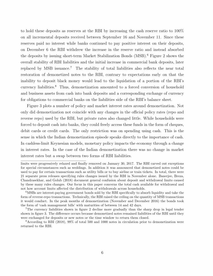
Cash and the Economy:Evidence from India’s Demonetization∗

Gabriel Chodorow-Reich Gita GopinathHarvard Harvard

Prachi Mishra Abhinav NarayananGoldman Sachs Reserve Bank of India

December 2018

Abstract

We analyze a unique episode in the history of monetary economics, the 2016 Indian“demonetization.” This policy made 86% of cash in circulation illegal tender overnight,with new notes gradually introduced over the next several months. We present a modelof demonetization where agents hold cash both to satisfy a cash-in-advance constraintand for tax evasion purposes. We test the predictions of the model in the cross-sectionof Indian districts using several novel data sets including: a data set containing thegeographic distribution of demonetized and new notes for causal inference; nightlightsdata and employment surveys to measure economic activity including in the informalsector; debit/credit cards and e-wallet transactions data; and banking data on depositand credit growth. Districts experiencing more severe demonetization had relativereductions in economic activity, faster adoption of alternative payment technologies,and lower bank credit growth. The cross-sectional responses cumulate to a contractionin employment and nightlights-based output due to demonetization of 2 p.p. and ofbank credit of 2 p.p. in 2016Q4 relative to their counterfactual paths, effects whichdissipate over the next few months. We use our model to show these cumulated effectsare a lower bound for the aggregate effects of demonetization. We conclude that unlikein the cashless limit of new-Keynesian models, in modern India cash serves an essentialrole in facilitating economic activity.

∗We would like to thank Martin Rama and Robert Carl Michael Beyer of the World Bank for sharing

night lights data, Tilottama Ghosh at the Earth Observation Group at NOAA for clarifying many basic

questions relating to the nightlights data, National Payments Corporation of India for providing data on

ATM and POS transactions, and Quantta for providing geocode coordinates. Gabriel Konigsberg and Anna

Stansbury provided excellent research assistance. Ms. Mishra was employed at the IMF at the time this

work was completed. The views expressed herein are those of the authors and not necessarily those of the

Reserve Bank of India, Goldman Sachs, or any other institution with which the authors are affiliated.

1 Introduction

Cash can serve an essential role and raise welfare by overcoming frictions in transactions such

as the lack of double coincidence of wants, limited commitment, and asymmetric information.

In the New Keynesian synthesis (Woodford, 2003), however, which is at the foundation of

modern monetary policy making, money only serves as a unit of account. In this so-called

cashless limit, outcomes depend on the interest rate set by monetary policy, with the details

of the change in money supply that accompany it essentially irrelevant. Instead, cash is an

inconvenience which constrains monetary policy by putting a floor on the nominal interest

rate and facilitates illegal activity and tax evasion (Rogoff, 2016).

In this paper we study the importance of the transaction role of cash by analyzing a

unique episode in the history of monetary economics. On November 8th, 2016, the gov-

ernment of India unexpectedly declared 86% of the existing currency in circulation illegal

tender, effective at midnight. Referred to as “demonetization,” this policy resulted in a

sharp decrease in the availability of cash which could be used in transactions because print-

ing press constraints prevented the immediate replacement of the demonetized currency with

new notes. Demonetization occurred in an otherwise stable macroeconomic environment and

did not affect other hallmarks of monetary policy such as the overall liabilities of the Re-

serve Bank of India (RBI) or the target interest rate. Thus, the experiment offers a unique

opportunity to observe the importance of cash as a facilitator of transactions.

We first present a model of demonetization to translate the policy into standard economics

and generate predictions. In the model, agents hold cash for two reasons. Firstly, because of

a cash-in-advance (CIA) constraint requiring money holdings to pay for expenditures, along

the lines of Lucas (1982), Lucas and Stokey (1987), and Svensson (1985). Secondly, because

holding cash reduces the effective tax rate by facilitating tax evasion. Demonetization in

the model amounts to a forced conversion of cash into less liquid bank deposits, which in

the presence of downward wage rigidity generates a decline in output, employment, and

borrowing by firms. Households also switch to non-cash forms of payment to attenuate the

impact of the cash shortage.

We then provide empirical evidence of the effects of demonetization. National time series

aggregates cannot answer this question because they have limited coverage of the informal,

cash-intensive sector of the economy and because other economic shocks occurred during

the period. Instead, we study the consequences of demonetization in the cross-section of

Indian districts. Using a comprehensive data set from the RBI containing the geographic

distribution of demonetized and new notes, we construct a local area demonetization shock

1

as the ratio of the arrival of new notes in an area to the quantity of demonetized notes

in that area. We present both narrative and statistical evidence that variation in these

demonetization shocks occurred essentially at random with respect to economic activity.

We study outcomes drawn from a number of different data sets, many of which have not

previously been used in academic research. We first show that districts which experienced

more severe demonetization shocks had much larger contractions in ATM withdrawals. The

link between currency availability and cash withdrawals both validates the usefulness of our

geographic shock measure and provides prima facie evidence of a cash shortfall.

We next show that demonetization had an adverse effect on real economic activity. Offi-

cial data on economic activity at a subnational level and at high frequency do not exist. We

use a new household survey of employment and satellite data on human-generated nightlight

activity to measure demonetization’s effects at the district level. Importantly, these variables

capture both formal and informal sector economic activity. Both variables show econom-

ically sharp, statistically highly significant contractions in areas experiencing more severe

demonetization shocks. The effects on real economic activity peak in the period immedi-

ately following the announcement and dissipate over the next few months as new currency

arrives. In terms of magnitude, comparing districts at the 10th and 90th percentiles of the

demonetization shock in the period immediately after the announcement, both variables map

into a difference in output of roughly 4.5 percentage points.

Our third set of results show the adoption of alternative forms of payment technology.

While the difference in output across districts is substantial, it is far less than the roughly

50 percentage point inter-decile difference in the amount of currency replaced. In our model,

this can occur if households endogenously found ways around using money to conduct trans-

actions, for example by switching to alternative payment methods like debit cards, credit

cards, and e-wallets or by convincing retailers to open an informal line of credit or to accept

old notes. We use data on the transacted value of two leading electronic payments methods,

e-wallet and point-of-service cards, to show that this substitution occurred. This pattern

also corroborates our identifying assumption as a confounding non-demonetization demand

shock would induce comovement across all payments mechanisms and output.

Finally, we show responses in the banking sector. Areas which experienced more severe

cash shortages had higher deposit growth as households could not withdraw money from their

bank accounts. Credit growth in these areas also slowed, providing additional corroborating

evidence of an effect on real activity.

Our results imply demonetization lowered the growth rate of economic activity by at least

2

2 p.p. in the quarter of demonetization. To reach this number, we first cumulate the cross-

sectional effects on employment and nightlights over districts. Next, our model suggests

that these cross-sectional estimates provide a lower bound for the aggregate consequences of

demonetization due to cross-district trade. Combining these two results yields a decline in

nightlights-based economic activity and of employment of 3 p.p. or more in November and

December of 2016 relative to the the counterfactual path, which translates into a decline in

the quarterly growth rate of 2 p.p. or more. Similarly, the effect on credit implies a 2 p.p.

or more decline in 2016Q4.1 We conclude that while the cashless limit may appropriately

describe economies with well developed financial markets, in modern India cash continues

to serve an essential role in facilitating economic activity.

We review related literature next. Section 2 contains institutional details of demonetiza-

tion. Section 3 presents the model and empirical predictions. Section 4 describes the data,

the construction of the geographic demonetization shocks, and the conditions for causal

interpretation of the analysis. Section 5 presents the results and Section 6 discusses the

aggregate implications.

Related literature. A few early studies have used descriptive statistics (RBI, 2017b; Kr-

ishnan and Siegel, 2017) or simple time series methods (Aggarwal and Narayanan, 2017;

Banerjee and Kala, 2017) to infer the effect of demonetization on the Indian economy. We

introduce a number of new data sets and a cross-sectional empirical approach to more cred-

ibly identify the causal effects of the policy. Methodologically, this approach relates to a

burgeoning literature using cross-sectional, regional variation to study macroeconomic top-

ics, as reviewed in Nakamura and Steinsson (2018) and Chodorow-Reich (Forthcoming).

This literature has so far avoided the topic of monetary policy because monetary policy is

determined at the national (or higher) level. In contrast, our setting contains large cross-

regional variation in the change in money. Ramey (2016) offers a forceful critique of time

series studies of the effect of money on output as restricted to studying small changes in

policy. Similar to Velde (2009) who traces the effects of large, overnight diminutions of coins

in 18th century France, we study a sudden and very large change in currency.

Our empirical results provide support for theoretical traditions which view money as

essential in that the presence of money makes possible superior allocations. We follow Lu-

cas (1982), Lucas and Stokey (1987), and Svensson (1985) in modeling the need for money

through a cash-in-advance (CIA) constraint. The “new monetarist perspective” (Williamson

1These are non-annualized numbers.

3

and Wright, 2010) instead introduces limited commitment and lack of double coincidence of

wants to create a problem which money alleviates.2 Agrawal (2018) provides a model of a

demonetization episode in this tradition. As noted by Kocherlakota (1998), any mechanism

which creates a record of transactions (“memory”) can substitute for money in a new mon-

etarist economy. We document empirically one such substitution – the switch to e-wallet

and POS payments technologies. Our model incorporates such substitution through an en-

dogenous threshold for the CIA constraint, making it immune along this dimension to an

otherwise clear example of the Lucas critique (Lucas, 1976) applying.3 In independent work,

Crouzet, Gupta, and Mezzanotti (2018) also examine the adoption of alternative payment

technology during demonetization and, like us, find persistent effects of demonetization on

e-wallet use. Whereas their paper focuses on the network externalities of payment technolo-

gies, we emphasize the interplay between adoption of alternative means of payment and the

effect on output.

Last, our paper sheds light on a policy debate around the possible benefits of moving to a

cashless economy. Rogoff (2016) articulates the societal costs of cash including putting a floor

on the nominal interest rate and facilitating illegal activity and tax evasion. Nonetheless,

he cautions that if it occurs a phase-out of cash should take place slowly and with ample

anticipation to allow households to adjust to other forms of payment. Our results accord

with these prescriptions.

2 Demonetization

On November 8, 2016, at 8:15pm local time, the Prime Minister of India announced in an

unscheduled national televised address that the two largest denomination notes, the 500

($7.5) and 1000 rupee ($15) notes, would cease to be legal tender, to be replaced by new

500 and 2000 notes. Effective at midnight, holders of the old notes could deposit them at

banks but could not use them in transactions. The stated objectives of the policy were to

target black money, reduce corruption, and remove fake currency notes. In the service of

these objectives, the government placed deposit limits on customers who did not comply

with “Know Your Customer” norms and set a deadline of December 31, 2016 for the return

2Lagos and Zhang (2018) argue theoretically that monetary models without money are generically poorapproximations even to highly developed credit economies.

3Alvarez and Lippi (2009) examine the impact of financial innovation on the demand for cash.

4

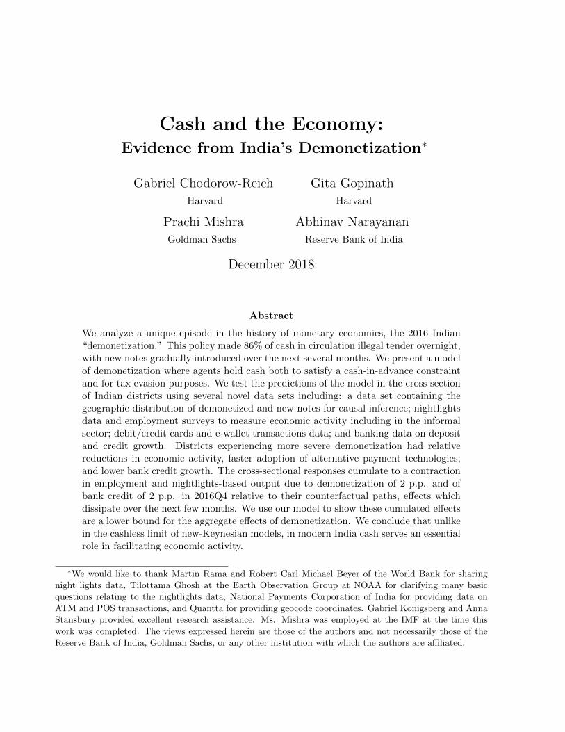
Figure 1: Large Denomination Legal Tender

0.10

0.20

0.30

0.40

0.50

0.60

0.70

0.80

0.90Sh

are

of P

re-D

emon

etiz

atio

n C

urre

ncy

Nov16

Dec16

Jan17

Feb17

Mar17

Apr17

May17

Jun17

Jul17

Aug17

Sep17

Oct17

Nov17

Dec17

Notes: The figure plots the value of old 500 and 1000 notes (before November 8, 2016) and new 500 and2000 notes (after November 8, 2016) as a share of total currency in circulation on November 4, 2016 usingthe currency chest data described below.

of old notes.4

Figure 3 shows the path of large legal tender denomination notes as a share of total pre-

announcement currency outstanding, using the currency chest data described below. The

old 500 and 1000 notes accounted for 86% of pre-demonetization currency. To maintain

secrecy prior to the policy’s announcement, the government did not print and distribute a

large quantity of new notes. Printing press constraints then prevented the government from

quickly replacing more than a fraction of this total with new notes. Thus, total currency

declined overnight by 75% and recovered only slowly over the next several months.

While the slow replacement of notes led to a decline in currency, it did not affect the

overall size of the RBI’s balance sheet or market interest rates. The immediate consequence

was to increase deposits at commercial banks as households deposited old notes but could

not freely withdraw new notes due to the cash shortage.5 The RBI initially required banks

4The December 31st limit applied to ordinary note holders. Non-resident Indian citizens could continueto deposit old notes until June 30, 2017. Customers who did not comply with the KYC norms could deposita maximum of Rs 50,000. While all commercial banks and urban cooperative banks were allowed to acceptdeposits in old currencies, district cooperative banks (DCCBs) were prohibited to do so.

5As we later show, the supply of new notes in a geographic area determined the total amount of with-drawals by households in that area. There were also legal limitations on withdrawals from individual ac-counts. The exchange of old for new notes was initially restricted to Rs 4000 ($60) per person per day, cashwithdrawals from bank accounts were initially limited to Rs. 10,000 ($150) per day and Rs 20,000 ($300) perweek, and withdrawals from ATM machines were initially restricted to Rs 2000 ($30) per day per card. These

5

to hold these deposits as reserves at the RBI by increasing the cash reserve ratio to 100%

on all incremental deposits received between September 16 and November 11. Since these

reserves paid no interest while banks continued to pay positive interest on their deposits,

on December 6 the RBI withdrew the increase in the reserve ratio and instead absorbed

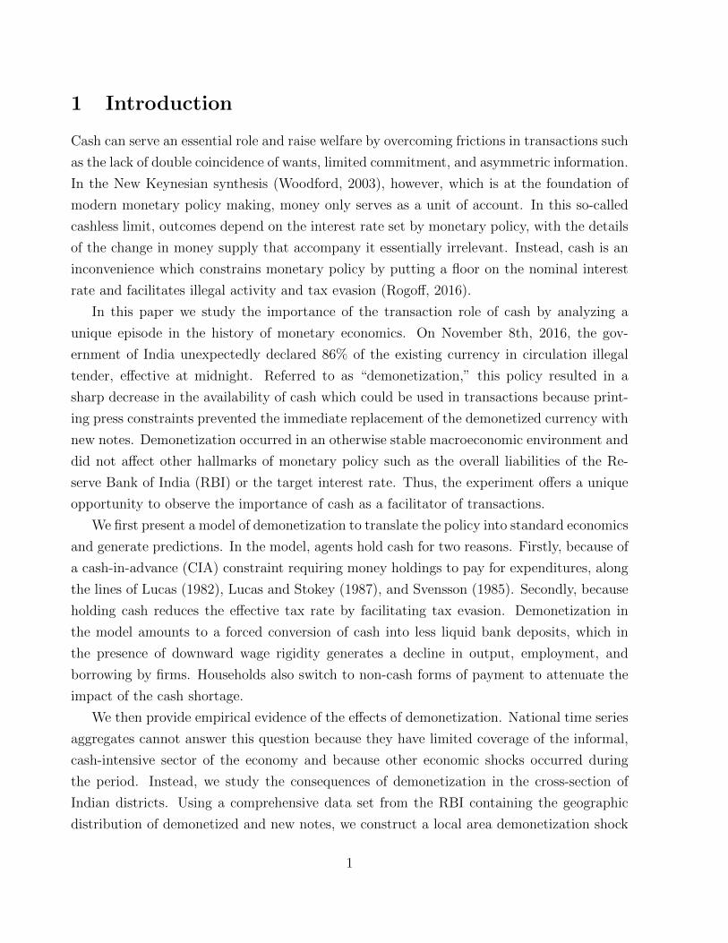
the deposits by issuing short-term Market Stabilization Bonds (MSB).6 Figure 2 shows the

overall stability of RBI liabilities and the initial increase in commercial bank deposits, later

replaced by MSB issuance.7 The stability of total liabilities also reflects the near total

restoration of demonetized notes to the RBI, contrary to expectations early on that the

inability to deposit black money would lead to the liquidation of a portion of the RBI’s

currency liabilities.8 Thus, demonetization amounted to a forced conversion of household

and business assets from cash into bank deposits and a corresponding exchange of currency

for obligations to commercial banks on the liabilities side of the RBI’s balance sheet.

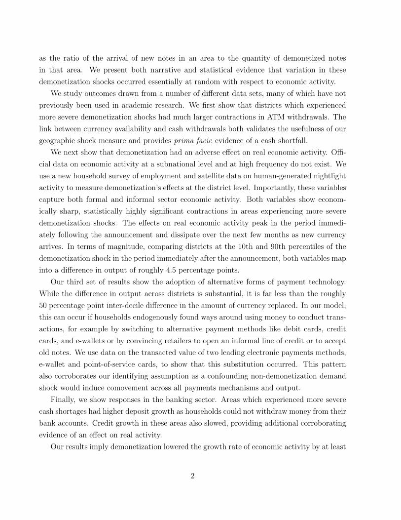
Figure 3 plots a number of policy and market interest rates around demonetization. Not

only did demonetization not coincide with any changes in the official policy rates (repo and

reverse repo) used by the RBI, but private rates also changed little. While households were

forced to deposit cash into banks, they could freely access these funds in the form of cheques,

debit cards or credit cards. The only restriction was on spending using cash. This is the

sense in which the Indian demonetization episode speaks directly to the importance of cash.

In cashless-limit Keynesian models, monetary policy impacts the economy through a change

in interest rates. In the case of the Indian demonetization there was no change in market

interest rates but a swap between two forms of RBI liabilities.

limits were progressively relaxed and finally removed on January 30, 2017. The RBI carved out exceptionsfor special circumstances such as weddings. In addition it was announced that demonetized notes could beused to pay for certain transactions such as utility bills or to buy airline or train tickets. In total, there were21 separate press releases specifying rules changes issued by the RBI in November alone. Banerjee, Breza,Chandrasekhar, and Golub (2018) document general confusion about deposit and withdrawal limits causedby these many rules changes. Our focus in this paper concerns the total cash available for withdrawal andnot how account limits affected the distribution of withdrawals across households.

6MSBs are interest-paying government bonds sold by the RBI specifically to absorb liquidity and take theform of reverse-repo transactions. Technically, the RBI raised the ceiling on the quantity of MSB transactionsit would conduct. In the peak months of demonetization (November and December 2016) the bonds tookthe form of ‘cash management bills’ with maturities of between 14 and 42 days.

7The currency liabilities shown in figure 2 decline more gradually than the sharp drop in legal tendershown in figure 3. The difference occurs because demonetized notes remained liabilities of the RBI until theywere exchanged for deposits or new notes or the time window to return them closed.

8According to RBI (2018), 99% of total 500 and 1000 notes in circulation prior to demonetization werereturned to the RBI.

6

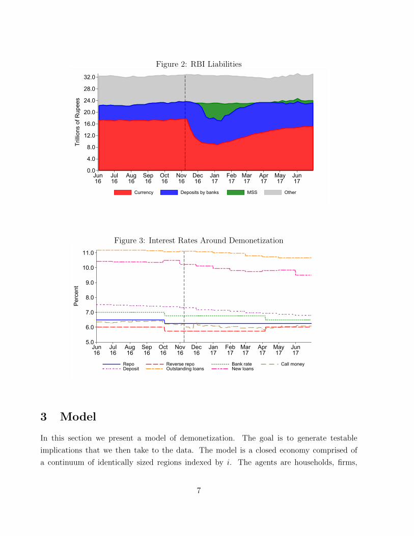
Figure 2: RBI Liabilities

0.0

4.0

8.0

12.0

16.0

20.0

24.0

28.0

32.0Tr

illion

s of

Rup

ees

Jun16

Jul16

Aug16

Sep16

Oct16

Nov16

Dec16

Jan17

Feb17

Mar17

Apr17

May17

Jun17

Currency Deposits by banks MSS Other

Figure 3: Interest Rates Around Demonetization

5.0

6.0

7.0

8.0

9.0

10.0

11.0

Perc

ent

Jun16

Jul16

Aug16

Sep16

Oct16

Nov16

Dec16

Jan17

Feb17

Mar17

Apr17

May17

Jun17

Repo Reverse repo Bank rate Call moneyDeposit Outstanding loans New loans

3 Model

In this section we present a model of demonetization. The goal is to generate testable

implications that we then take to the data. The model is a closed economy comprised of

a continuum of identically sized regions indexed by i. The agents are households, firms,

7

banks, and the government. Each region produces a non-traded good and a unique variety

of a good ω which is traded freely across regions. We will consider both the extremes of

perfect labor mobility and perfectly immobile labor. An important friction in the labor

market is downward nominal wage rigidity as in Schmitt-Grohe and Uribe (2016) and owing

to which equilibrium employment can fall short of inelastically supplied labor and give rise

to involuntary unemployment. This assumption is consistent with the evidence in Kaur,

Supreet (forthcoming) for wages in India.

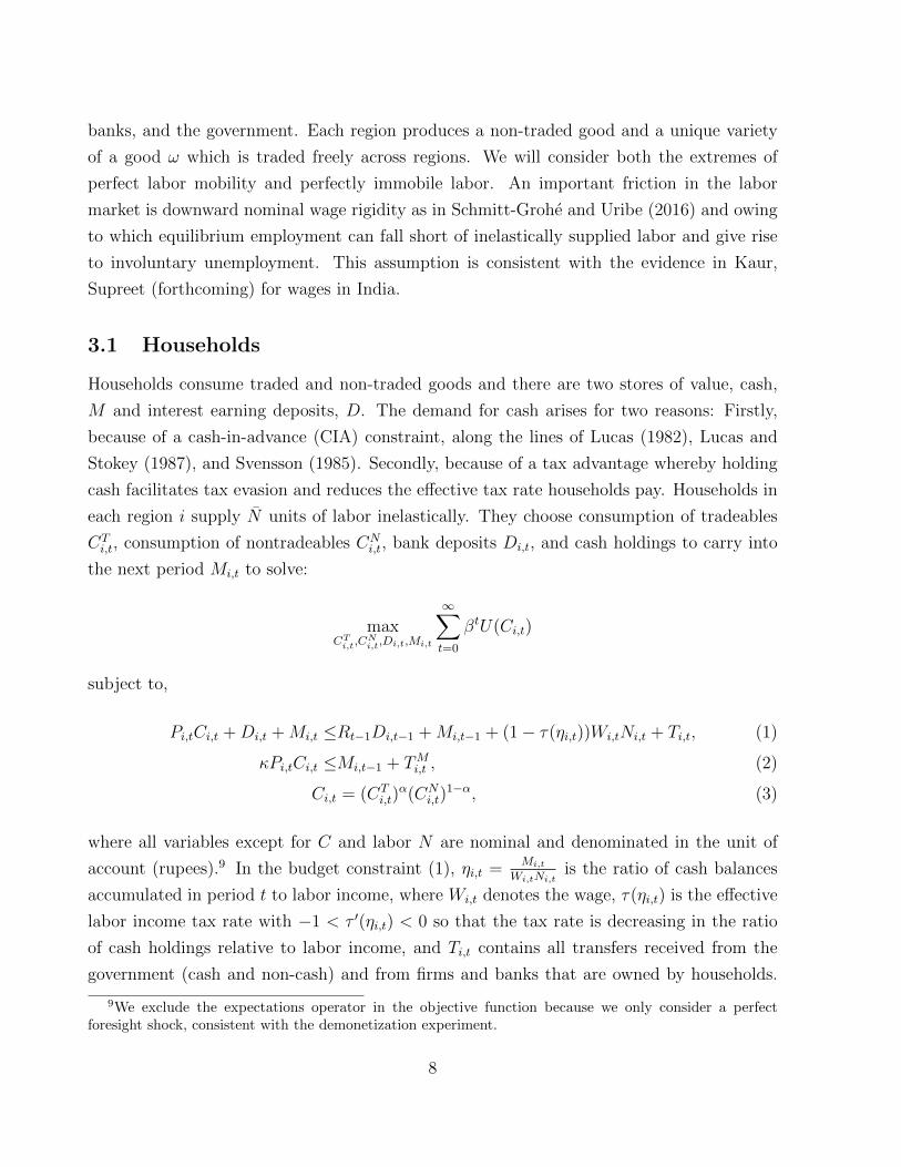
3.1 Households

Households consume traded and non-traded goods and there are two stores of value, cash,

M and interest earning deposits, D. The demand for cash arises for two reasons: Firstly,

because of a cash-in-advance (CIA) constraint, along the lines of Lucas (1982), Lucas and

Stokey (1987), and Svensson (1985). Secondly, because of a tax advantage whereby holding

cash facilitates tax evasion and reduces the effective tax rate households pay. Households in

each region i supply N units of labor inelastically. They choose consumption of tradeables

CTi,t, consumption of nontradeables CN

i,t, bank deposits Di,t, and cash holdings to carry into

the next period Mi,t to solve:

maxCTi,t,C

Ni,t,Di,t,Mi,t

∞∑t=0

βtU(Ci,t)

subject to,

Pi,tCi,t +Di,t +Mi,t ≤Rt−1Di,t−1 +Mi,t−1 + (1− τ(ηi,t))Wi,tNi,t + Ti,t, (1)

κPi,tCi,t ≤Mi,t−1 + TMi,t , (2)

Ci,t = (CTi,t)

α(CNi,t)

1−α, (3)

where all variables except for C and labor N are nominal and denominated in the unit of

account (rupees).9 In the budget constraint (1), ηi,t =Mi,t

Wi,tNi,tis the ratio of cash balances

accumulated in period t to labor income, where Wi,t denotes the wage, τ(ηi,t) is the effective

labor income tax rate with −1 < τ ′(ηi,t) < 0 so that the tax rate is decreasing in the ratio

of cash holdings relative to labor income, and Ti,t contains all transfers received from the

government (cash and non-cash) and from firms and banks that are owned by households.

9We exclude the expectations operator in the objective function because we only consider a perfectforesight shock, consistent with the demonetization experiment.

8

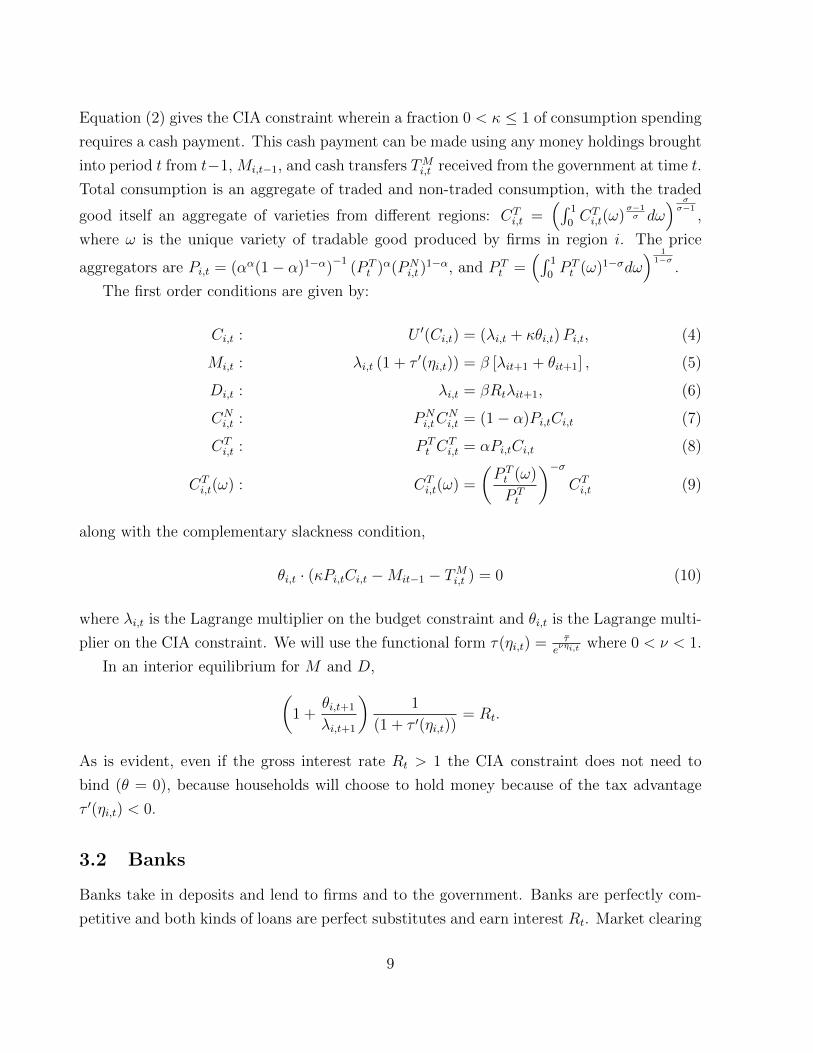
Equation (2) gives the CIA constraint wherein a fraction 0 < κ ≤ 1 of consumption spending

requires a cash payment. This cash payment can be made using any money holdings brought

into period t from t−1, Mi,t−1, and cash transfers TMi,t received from the government at time t.

Total consumption is an aggregate of traded and non-traded consumption, with the traded

good itself an aggregate of varieties from different regions: CTi,t =

(∫ 1

0CTi,t(ω)

σ−1σ dω

) σσ−1

,

where ω is the unique variety of tradable good produced by firms in region i. The price

aggregators are Pi,t = (αα(1− α)1−α)−1

(P Tt )α(PN

i,t )1−α, and P T

t =(∫ 1

0P Tt (ω)1−σdω

) 11−σ

.

The first order conditions are given by:

Ci,t : U ′(Ci,t) = (λi,t + κθi,t)Pi,t, (4)

Mi,t : λi,t (1 + τ ′(ηi,t)) = β [λit+1 + θit+1] , (5)

Di,t : λi,t = βRtλit+1, (6)

CNi,t : PN

i,tCNi,t = (1− α)Pi,tCi,t (7)

CTi,t : P T

t CTi,t = αPi,tCi,t (8)

CTi,t(ω) : CT

i,t(ω) =

(P Tt (ω)

P Tt

)−σCTi,t (9)

along with the complementary slackness condition,

θi,t · (κPi,tCi,t −Mit−1 − TMi,t ) = 0 (10)

where λi,t is the Lagrange multiplier on the budget constraint and θi,t is the Lagrange multi-

plier on the CIA constraint. We will use the functional form τ(ηi,t) = τeνηi,t

where 0 < ν < 1.

In an interior equilibrium for M and D,(1 +

θi,t+1

λi,t+1

)1

(1 + τ ′(ηi,t))= Rt.

As is evident, even if the gross interest rate Rt > 1 the CIA constraint does not need to

bind (θ = 0), because households will choose to hold money because of the tax advantage

τ ′(ηi,t) < 0.

3.2 Banks

Banks take in deposits and lend to firms and to the government. Banks are perfectly com-

petitive and both kinds of loans are perfect substitutes and earn interest Rt. Market clearing

9

requires ∫i

Afi,tdi+ Agt =

∫i

Di,tdi,

where Afi,t is lending to firms and Agt is lending to the government.

3.3 Firms

Firms in both the tradable and non-tradable sectors are perfectly competitive. Each firm

faces a working capital constraint where a fraction ϕ of the wage bill needs to be paid in

advance. Firms take a loan Bfi,t = ϕWi,tNi,t from the bank for this purpose. The production

function for either good is Yt = Nt. With perfect competition price equals marginal cost:

P Tt (ω) = PN

i,t = (1 + ϕ(Rt − 1))Wi,t.

For now we have indexed the wage rate by i to allow for immobile labor.

3.4 Downward Wage Rigidity

As in Schmitt-Grohe and Uribe (2016) the main friction is that nominal wages are down-

wardly rigid by a factor 0 < γ ≤ 1,

Wi,t ≥ γWit−1, (11)

which can prevent full employment. If γ = 1 then nominal wages can never fall. The evidence

in Kaur, Supreet (forthcoming) implies γ = 1. When the constraint does not bind, Ni,t = N .

Consequently we have the complementary slackness condition,

(N −Ni,t)(Wi,t − γWit−1) = 0

when labor is immobile across regions, and

(N −Nt)(Wt − γWt−1) = 0

when labor is perfectly mobile.

10

3.5 Government

The consolidated budget constraint of the government satisfies,∫ 1

0

(M s

i,t +Bgi,t + τ(ηi,t)Wi,tNi,t

)di =

∫ 1

0

(TMi,t + T gi,t +M s

i,t−1 +Rt−1Bgi,t−1

)di

TMi,t = M si,t −M s

i,t−1 ∀i ∈ [0, 1],

whereBgi,t denotes government bonds issued in period t. The government raises funds through

money creation, debt issuance, and labor income taxes, all of which is transferred to house-

holds.

3.6 Market Clearing

Traded goods markets clear countrywide,∫iCTi,t(ω)di = Y T

t (ω). Non-traded goods markets

clear by region, CNi,t = Y N

i,t . Further, Afi,t = Bfi,t, A

gt = Bg

t and M si,t = Mi,t. M

si,t is the cash

that is supplied to region i.

3.7 Pre-Demonetization Steady State

The economy in period −1 is in a steady state where because of tax evasion incentives the

CIA does not bind, M−1 > κP−1C−1. This requires that κ(1 + ϕ( 1β− 1)) < 1

νln(

ντ1−β

), that

is, that the tax rate τ is sufficiently high relative to the interest rate and to the fraction

of spending that needs to be undertaken in cash κ. This assumption reflects the argument

made by the Indian government that an important fraction of pre-demonetization cash was

‘black money’ held for tax evasion purposes.

Proposition 1 Pre-demonetization steady state

In period -1 all regions are in a symmetric zero inflation steady state with M s = M−1, and

1. The economy is in full employment:

N−1 = N , Y T−1 = NT

−1 = αN, Y N−1 = NN

−1 = (1− α)N . (12)

2. Real money balances are increasing in the level of consumption C and in the labor

11

income tax τ and decreasing in the interest rate R−1 = 1/β:

M−1

P−1

=η−1C−1

(1 + ϕ(R−1 − 1)), η−1 =

1

νln

(ντ

1− (1/R−1)

). (13)

3. Nominal wages and prices are given by:

W−1 =M−1

Nη−1

, P T−1 = PN

−1 = (1 + ϕ(β−1 − 1))M−1

Nη−1

. (14)

�

With a constant level of money supply in the economy, the wage friction does not bind and

the economy is in full employment with a fraction α of labor employed in the traded sector

and (1− α) in the non-traded sector.

3.8 Demonetization

At the start of period 0 the government (unexpectedly) announces that only a fraction of cash

which households carry into period 0 is legal tender and can be used for transaction purposes

(demonetization) and requires the remaining cash be deposited at the pre-fixed interest rate

of R−1. This policy corresponds to a drop in available money balances in period 0, forcing

households off their deposit Euler equation (6). At the start of period 1 demonetization ends

and the money supply returns to the level required to maintain full employment. There is no

uncertainty following the announcement of the demonetization shock so household decisions

at the end of period 0 reflect the anticipated cash infusion.

We first describe the solution for the case when the demonetization is uniform across all

regions in 0. The solution remains symmetric and the path of cash is such that the CIA and

wage constraints bind in period 0 before becoming loose again in period 1 and after.10

Proposition 2 Uniform demonetization

Let Z = M s0/M

s−1 = M0/M−1 where 0 < Z < 1 so that the CIA binds and the wage constraint

10As long as the CIA binds we can solve for the outcomes in period 0 without the solutions for period 1and beyond. This is because interest rates are pre-fixed at R−1 and the deposit Euler equation and moneyEuler equations are irrelevant. To verify the conditions under which the CIA binds we need to solve fully forthe dynamic solution. We provide the full solution in the appendix. Due to one-sided wage rigidity, thereare multiple values for M in period 1 which guarantee full employment and we choose the minimal suchvalue. This value requires an equilibrium wage W1 > γW0 = γ2W−1 at which the downward wage rigidityis not binding. If γ ≈ 1 then M1 ≈M−1 and the cash to GDP ratio returns to the pre-demonetization level.

12

binds, that is κP0C0 = M0 and W0 = γW−1. If Z is sufficiently low relative to the downward

rigidity of wages,11 Z · η−1

κ(1+ϕ(β−1−1))< γ, then:

1. Output and employment declines:

Y T0 = NT

0 =Z

γ· η−1

κ(1 + ϕ(β−1 − 1))· αN,

Y N0 = NN

0 =Z

γ· η−1

κ(1 + ϕ(β−1 − 1))· (1− α)N ,

Y0

Y−1

=Z

γ· η−1

κ(1 + ϕ(β−1 − 1)). (15)

2. Lending by banks to firms decline:

Bf0

P0

=ϕN0

(1 + ϕ(R−1 − 1))<Bf−1

P−1

. (16)

3. Nominal wages and prices are given by:

W0 = γW−1, P T0 = PN

0 = (1 + ϕ(β−1 − 1))γW−1. (17)

�

The solution for output features a proportional decline between output and Z. This

proportionality arises because of the binding CIA constraint M0 = κP0C0 which tightly

links cash in period 0 to output Y0 = C0.12 We also have that the ratio of money holdings to

labor income falls η0 < η−1 owing to which the effective tax rate rises τ0 > τ1, but this is not

distortionary because of perfectly inelastic labor supply. The shadow interest rate, which is

the interest rate consistent with the deposit Euler equation, rises: Rs0 ≡ λ0

βλ1= 1

(1−ντ(η0))>

1(1−ντ(η−1))

= R−1.

We next consider the case where the decline in M is not uniform across regions, as we

will exploit in our empirical work. The government reduces the supply of cash in region i in

11Recall that for the CIA not to bind in period -1 we require that η−1

κ(1+ϕ(β−1−1)) > 1 which means that we

need Zγ to be sufficiently lower than 1 to compensate for this. The reason it does not depend only on Z/γ

is because the nominal wage when the CIA binds is different from when the CIA does not bind.12To see this, start from the binding CIA constraint M0 = κP0C0 and substitute the equilibirium con-

ditions P0 = (1 + ϕ (R−1 − 1))W0 =(1 + ϕ

(β−1 − 1

))γW−1 and Yt = Ct = Nt and the definitions

η−1 = M−1/ (W−1N−1) and Z = M0/M−1 to arrive at equation (15) in the proposition. As should beclear, while in our setup P0 is sticky downwards because of the downward wage rigidity, any nominal frictionwhich keeps P0 from falling will result in a similar expression.

13

a proportion Zi ∈ (0, 1), i.e. M si,0 = ZiM

s−1 such that Zi = Z(1 + εi) and where

∫iεidi = 0.

We assume households cannot undo the heterogeneous distribution of cash across regions

through financial markets.

Proposition 3 Non-uniform demonetization

If the drop in each region is sufficient to make the CIA constraint and wage constraint bind

in all regions, that is, κPi,0Ci,0 = Mi,0 and Wi,0 = γW−1 ∀i, then:

1. Regions with higher Zi have smaller declines in output. The differential is increasing

in the size of the non-traded sector:

Yi,0Yi,−1

=Y T

0 (ω) + Y Ni,0

Yi,−1

=αZ + (1− α)Zi

γ· η−1

κ(1 + ϕ(β−1 − 1)). (18)

2. Borrowing by firms falls by less in regions with higher Zi:

Bfi,0

P0

=ϕYi0

(1 + ϕ(β−1 − 1)). (19)

3. Nominal wages and prices are given by:

Wi,0 = γW−1, P T0 = PN

i,0 = (1 + ϕ(β−1 − 1))γW−1. (20)

�

The impact of the idiosyncratic component of the money shock is decreasing in the size

of the traded sector. As α → 1 there is no cross-regional variation in output. Regional

employment tracks regional output and, because of downward wage rigidity, the wage is

equalized across regions regardless of whether there is labor mobility. Bank credit growth,

Bfi,t/P0, is increasing in Zi. If all banks are national banks and market clearing is given by∫iAfi,tdi + Agt =

∫iDi,tdi then there is no necessary relation between local demand for loans

and loans extended by banks. If however banks have a location bias then there is differential

loan growth. Alternatively, a vanishingly small cost to firms that borrow from banks outside

their regions (or of banks that lend outside their region of location), given that interest rates

are the same, would generate a greater decline in credit creation by banks located in a region

with a smaller Zi.

14

3.9 Endogenous κ

We now extend the model in one important dimension: we allow households to endogenously

change κ by investing in a ‘finance’ technology fi,t to lower their dependence on cash transac-

tions. This investment encompasses a broad range of actions that households can undertake

including switching to alternative payment methods like debit cards, credit cards, and e-

wallets and convincing retailers to open an informal line of credit or to accept old notes.

The endogenous κ will allow the model to better match our empirical results by breaking

the unit elasticity between M and output in equation (15).

Specifically, κ(fi,t) is such that κ′(fi,t) < 0, κ(0) = κ. Making this investment entails a

utility loss h(fi,t) such that h′(fi,t) > 0, h′′(fi,t) ≥ 0, h(0) = 0. The household’s objective

function is now given by,

maxCTi,t,C

Ni,t,Di,t,Mi,t,fi,t

∞∑t=0

βt [U(Ci,t)− h(fi,t)]

and the CIA constraint takes the form,

κ(fi,t)Pi,tCi,t ≤Mi,t−1 + TMi,t . (21)

The budget constraint remains unchanged. In addition to the F.O.C listed previously (4-9)

(where κ is now an endogenous variable) we have the condition,

h′(fi,t) = −θi,tκ′(fi,t)Pi,tCi,t

according to which households will invest in the finance technology if the CIA constraint

binds and not otherwise. It follows that households do not invest in the finance technology

in periods −1 and 1 and in these periods κ = κ while they do invest in the period of

demonetization.

The full solution requires solving for θi,0, fi,0, ηi,0 using the following three equations.

θi,0 =1

ZiM−1

− 1

κ(fi,0)

βλi,11 + τ ′(ηi,0)

ηi,0 =Zi(1 + ϕ(β−1 − 1))

αI + (1− α) Ziκ(fi,0)

θi,0ZiM−1 = −h′(fi,0)κ(fi,0)

κ′(fi,0)

15

0 0.1 0.2 0.3 0.4 0.5 0.6 0.7Zi

0

0.05

0.1

0.15

0.2

0.25

f i,0

(a) Financial Services

0 0.1 0.2 0.3 0.4 0.5 0.6 0.7Zi

0

0.1

0.2

0.3

0.4

0.5

0.6

0.7

0.8

Effective cash reduction, Mi,0

/ (fi,0

)

Actual cash reduction, Zi

(b) Effective Cash Shortage

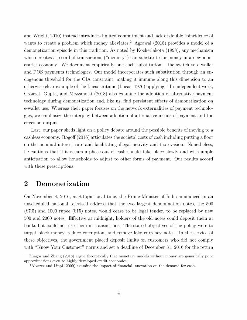
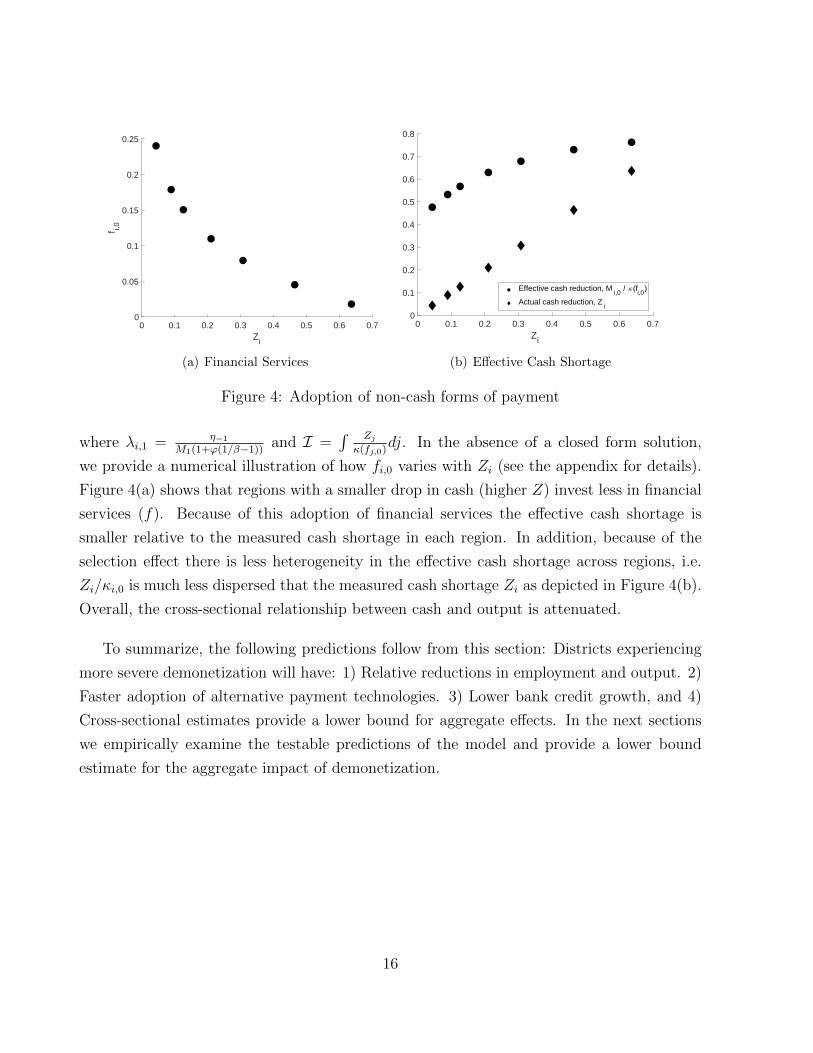
Figure 4: Adoption of non-cash forms of payment

where λi,1 = η−1

M1(1+ϕ(1/β−1))and I =

∫ Zjκ(fj,0)

dj. In the absence of a closed form solution,

we provide a numerical illustration of how fi,0 varies with Zi (see the appendix for details).

Figure 4(a) shows that regions with a smaller drop in cash (higher Z) invest less in financial

services (f). Because of this adoption of financial services the effective cash shortage is

smaller relative to the measured cash shortage in each region. In addition, because of the

selection effect there is less heterogeneity in the effective cash shortage across regions, i.e.

Zi/κi,0 is much less dispersed that the measured cash shortage Zi as depicted in Figure 4(b).

Overall, the cross-sectional relationship between cash and output is attenuated.

To summarize, the following predictions follow from this section: Districts experiencing

more severe demonetization will have: 1) Relative reductions in employment and output. 2)

Faster adoption of alternative payment technologies. 3) Lower bank credit growth, and 4)

Cross-sectional estimates provide a lower bound for aggregate effects. In the next sections

we empirically examine the testable predictions of the model and provide a lower bound

estimate for the aggregate impact of demonetization.

16

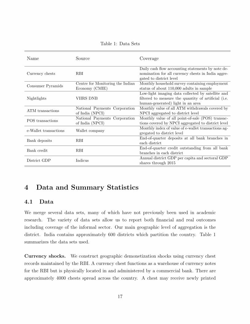
Table 1: Data Sets

Name Source Coverage

Currency chests RBIDaily cash flow accounting statements by note de-nomination for all currency chests in India aggre-gated to district level

Consumer PyramidsCentre for Monitoring the IndianEconomy (CMIE)

Monthly household survey containing employmentstatus of about 110,000 adults in sample

Nightlights VIIRS DNBLow-light imaging data collected by satellite andfiltered to measure the quantity of artificial (i.e.human-generated) light in an area

ATM transactionsNational Payments Corporationof India (NPCI)

Monthly value of all ATM withdrawals covered byNPCI aggregated to district level

POS transactionsNational Payments Corporationof India (NPCI)

Monthly value of all point-of-sale (POS) transac-tions covered by NPCI aggregated to district level

e-Wallet transactions Wallet companyMonthly index of value of e-wallet transactions ag-gregated to district level

Bank deposits RBIEnd-of-quarter deposits at all bank branches ineach district

Bank credit RBIEnd-of-quarter credit outstanding from all bankbranches in each district

District GDP IndicusAnnual district GDP per capita and sectoral GDPshares through 2015

4 Data and Summary Statistics

4.1 Data

We merge several data sets, many of which have not previously been used in academic

research. The variety of data sets allow us to report both financial and real outcomes

including coverage of the informal sector. Our main geographic level of aggregation is the

district. India contains approximately 600 districts which partition the country. Table 1

summarizes the data sets used.

Currency shocks. We construct geographic demonetization shocks using currency chest

records maintained by the RBI. A currency chest functions as a warehouse of currency notes

for the RBI but is physically located in and administered by a commercial bank. There are

approximately 4000 chests spread across the country. A chest may receive newly printed

17

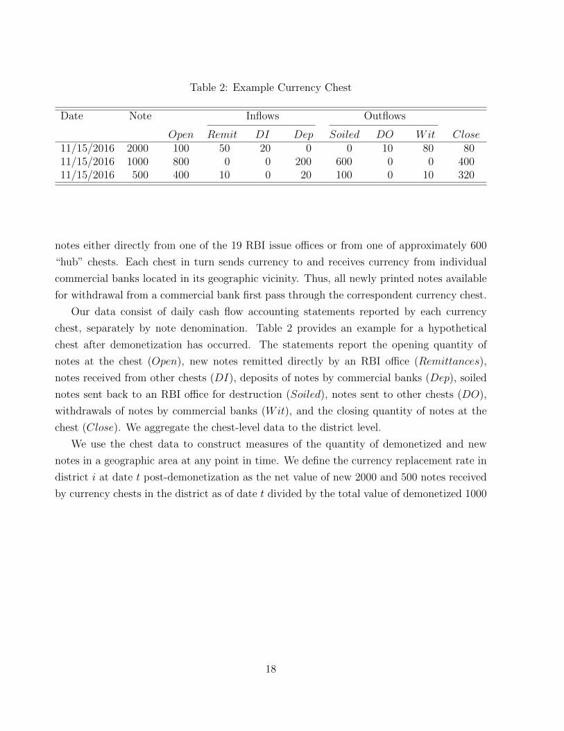
Table 2: Example Currency Chest

Date Note Inflows Outflows

Open Remit DI Dep Soiled DO Wit Close11/15/2016 2000 100 50 20 0 0 10 80 8011/15/2016 1000 800 0 0 200 600 0 0 40011/15/2016 500 400 10 0 20 100 0 10 320

notes either directly from one of the 19 RBI issue offices or from one of approximately 600

“hub” chests. Each chest in turn sends currency to and receives currency from individual

commercial banks located in its geographic vicinity. Thus, all newly printed notes available

for withdrawal from a commercial bank first pass through the correspondent currency chest.

Our data consist of daily cash flow accounting statements reported by each currency

chest, separately by note denomination. Table 2 provides an example for a hypothetical

chest after demonetization has occurred. The statements report the opening quantity of

notes at the chest (Open), new notes remitted directly by an RBI office (Remittances),

notes received from other chests (DI), deposits of notes by commercial banks (Dep), soiled

notes sent back to an RBI office for destruction (Soiled), notes sent to other chests (DO),

withdrawals of notes by commercial banks (Wit), and the closing quantity of notes at the

chest (Close). We aggregate the chest-level data to the district level.

We use the chest data to construct measures of the quantity of demonetized and new

notes in a geographic area at any point in time. We define the currency replacement rate in

district i at date t post-demonetization as the net value of new 2000 and 500 notes received

by currency chests in the district as of date t divided by the total value of demonetized 1000

18

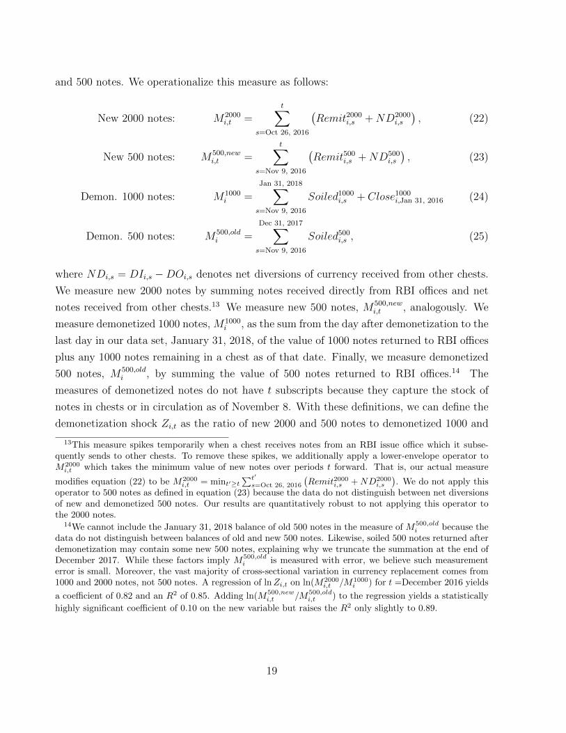
and 500 notes. We operationalize this measure as follows:

New 2000 notes: M2000i,t =

t∑s=Oct 26, 2016

(Remit2000

i,s +ND2000i,s

), (22)

New 500 notes: M500,newi,t =

t∑s=Nov 9, 2016

(Remit500

i,s +ND500i,s

), (23)

Demon. 1000 notes: M1000i =

Jan 31, 2018∑s=Nov 9, 2016

Soiled1000i,s + Close1000

i,Jan 31, 2016 (24)

Demon. 500 notes: M500,oldi =

Dec 31, 2017∑s=Nov 9, 2016

Soiled500i,s , (25)

where NDi,s = DIi,s −DOi,s denotes net diversions of currency received from other chests.

We measure new 2000 notes by summing notes received directly from RBI offices and net

notes received from other chests.13 We measure new 500 notes, M500,newi,t , analogously. We

measure demonetized 1000 notes, M1000i , as the sum from the day after demonetization to the

last day in our data set, January 31, 2018, of the value of 1000 notes returned to RBI offices

plus any 1000 notes remaining in a chest as of that date. Finally, we measure demonetized

500 notes, M500,oldi , by summing the value of 500 notes returned to RBI offices.14 The

measures of demonetized notes do not have t subscripts because they capture the stock of

notes in chests or in circulation as of November 8. With these definitions, we can define the

demonetization shock Zi,t as the ratio of new 2000 and 500 notes to demonetized 1000 and

13This measure spikes temporarily when a chest receives notes from an RBI issue office which it subse-quently sends to other chests. To remove these spikes, we additionally apply a lower-envelope operator toM2000i,t which takes the minimum value of new notes over periods t forward. That is, our actual measure

modifies equation (22) to be M2000i,t = mint′≥t

∑t′

s=Oct 26, 2016

(Remit2000i,s +ND2000

i,s

). We do not apply this

operator to 500 notes as defined in equation (23) because the data do not distinguish between net diversionsof new and demonetized 500 notes. Our results are quantitatively robust to not applying this operator tothe 2000 notes.

14We cannot include the January 31, 2018 balance of old 500 notes in the measure of M500,oldi because the

data do not distinguish between balances of old and new 500 notes. Likewise, soiled 500 notes returned afterdemonetization may contain some new 500 notes, explaining why we truncate the summation at the end ofDecember 2017. While these factors imply M500,old

i is measured with error, we believe such measurementerror is small. Moreover, the vast majority of cross-sectional variation in currency replacement comes from1000 and 2000 notes, not 500 notes. A regression of lnZi,t on ln(M2000

i,t /M1000i ) for t =December 2016 yields

a coefficient of 0.82 and an R2 of 0.85. Adding ln(M500,newi,t /M500,old

i,t ) to the regression yields a statistically

highly significant coefficient of 0.10 on the new variable but raises the R2 only slightly to 0.89.

19

500 notes:

Zi,t =M2000

i,t +M500,newi,t

M1000i +M500,old

i

. (26)

To remove districts with implausible replacement rates, we drop observations with Zi,t <

0, M500,oldi ≤ 0, or where

∑ts=Nov 9, 2016

(Withdrawals2000

i,s −Deposits2000i,s

)< 0 or differs

from M2000i,t by more than a factor of 3. That is, we require that new currency arriving

in a district be non-negative, that we observe a positive quantity of old 500 notes, that

cumulative deposits of 2000 notes by commercial banks not exceed cumulative withdrawals,

and that cumulative withdrawals net of deposits (i.e. net new 2000 notes actually received by

commercial banks) not differ from arrivals of new 2000 notes by too much.15 Applying these

criteria removes 47 of 591 districts which collectively contain less than 3% of demonetized

currency.

Employment. We obtain data on employment status from Consumer Pyramids for the

period January 2016 to October 2017. Unlike countries such as the United States, India does

not have a governmental monthly household survey or a monthly survey of establishments.16

The Centre for Monitoring the Indian Economy, a private organization, conducts a nationally

representative household survey referred to as Consumer Pyramids, which includes questions

on employment status similar to those asked in the Current Population Survey (CPS) in the

United States. Specifically, an individual counts as employed if on the day of the survey or

the day prior, the individual (i) did any paid work, (ii) was on paid or unpaid leave, (iii) was

not working because his/her workplace was temporarily shut down for maintenance or labor

dispute but expected to resume work within 15 days, (iv) owned a business in operation, or

(v) assisted in a family business. The survey covers roughly 110,000 adults (persons 15+)

per month, comparable to the sample size (although not the coverage rate) of the CPS.17

15Cumulative withdrawals net of deposits may differ from new arrivals of notes because currency withdrawnby a commerical bank in one district may go to a customer who re-deposits the notes in a bank in adifferent district. However, large discrepancies between the measures are rare and signal some restriction onwithdrawals which we do not observe.

16In April 2018 the Central Statistics Office began reporting monthly employment counts for formal sectorfirms based on administrative tax records, with data back to September 2017. The non-coverage of thedemonetization period or of informal sector employment make these data inappropriate for our analysis.

17The survey shares other similarities with the CPS and the Survey of Income and Program Participation(SIPP), such as the use of a stratefied sampling design (based on the 2011 Census) and a rotation structurewherein individual sampling units enter the survey every four months. The survey does not include any unitsfrom the following states or union territories: Arunachal Pradesh, Nagaland, Manipur, Mizoram, Tripura,Meghalaya, Sikkim, Andaman & Nicobar Islands, Dadra & Nagar Haveli, Lakshadweep and Daman and Diu.

20

We construct district-month measures of employment and population by aggregating the

individual observations using the survey weights. This step introduces four complications.

First, while the survey has national representation, it does not field in every district in every

month. Rather, it uses a rotation schedule wherein each primary sampling unit (a town or

village) with households in the sample gets visited once every four months. This pattern

means that most districts appear in the sample only once every four months, with larger

districts surveyed more frequently. The typical month therefore contains observations drawn

from roughly 150 districts. For this reason, we pool over adjoining months to increase the

sample size. Second, the survey is in the field continuously over the course of a month and we

do not know the exact interview date for each respondent. We exclude November 2016 from

the analysis since responses in that month mix pre-demonetization and post-demonetization

outcomes. Third, the survey weights do not aggregate to estimates of district population

which are consistent across months. We therefore use the ratio of total employed to persons

15 and older as our main outcome. Finally, we weight regressions using this variable by the

number of individual-level observations in the district to reflect the aggregation step.

Nightlights. Our second measure of real activity following demonetization is the change

in nightlight intensity. Nightlight intensity refers to low-light imaging data collected by

satellite and filtered to measure the quantity of artificial (i.e. human-generated) light in an

area. Such data have been used to augment official measures of output and output growth

and to generate estimates for areas or periods where official data are unavailable (Henderson,

Storeygard, and Weil, 2012). We use the VIIRS DNB data collected by NOAA using the

Suomi National Polar Partnership satellite which was launched in 2011 (Elvidge, Baugh,

Zhizhin, Hsu, and Ghosh, 2017). Despite the filtering, some stray light remain in these data.

NOAA provide annual composites which contain additional processing to remove such stray

light. We follow World Bank (2017) in removing cells (roughly 0.5km2) for which the annual

average of the data differ substantially from the annual composites before aggregating to the

district level. The resulting data are monthly frequency and contain substantial seasonality.

We seasonally adjust the data in both levels and logs by regressing nightlights on district-

specific linear time trends and month categorical variables over the period April 2012 to

March 2016, remove the month-specific factors, and then keep the series for each district

(unadjusted, adjusted in levels, adjusted in logs) with the smallest variance. This procedure

uses only data from before demonetization to perform the seasonal adjustment. Finally, we

aggregate the monthly data to quarterly to remove very high frequency volatility, dropping

21

October 2016 from 2016Q4 so that 2016Q4 is (almost entirely) post-demonetization.

ATM/POS. We obtain monthly data for the period January 2016 to June 2017 on the

value of ATM withdrawals and point-of-sale (POS) transactions by PIN code from National

Payments Corporation of India (NPCI), an umbrella organization set up by the RBI to

operate retail payments systems. A POS terminal is a device which enables payment by

credit or debit card over a telephone line or internet connection. We aggregate the data to

the district level using a concordance file from the post office. Where a PIN code covers

multiple districts, we assign the district based on the location of the main post office in the

district.

E-Wallet. We obtain monthly indexes of the total value of e-wallet transactions by district

from a wallet company for the period September 2016 to July 2017. E-Wallet technology

functions similar to pre-paid cards.18

Bank deposits and credit. We obtain publicly available end-of-quarter data on bank

deposits and credit outstanding by district from the RBI Quarterly Statistics on Deposits

and Credit of Scheduled Commercial Banks. These data come from branch-level reporting.

Therefore, district-level deposits correspond to deposits in accounts opened at branches

within the district. Likewise, district-level credit means loans granted by loan officers at

branches within the district regardless of the location of the borrower.

GDP and population. We obtain district-level measures of GDP, sectoral GDP, and

population from Indicus, a private data firm, and use these data to convert various series

to a per capita basis and as control variables below. We use data from 2015, the last year

of data available, in our analysis. We obtain national quarterly seasonally-adjusted nominal

and real GDP from OECD.19

18The wallet company issued the following disclaimer:“Wallet company shared only normalized data onpayments to merchants at an aggregate level for academic research. No user data has been shared in anyform. Wallet company does not have any role in drawing inferences of the study and the views expressed inthe study are solely of the authors.”

19The Indian Ministry of Statistics does not publish a seasonally-adjusted measure of quarterly GDP. TheOECD series closely mirrors that obtained by applying Census X12 to the unadjusted data.

22

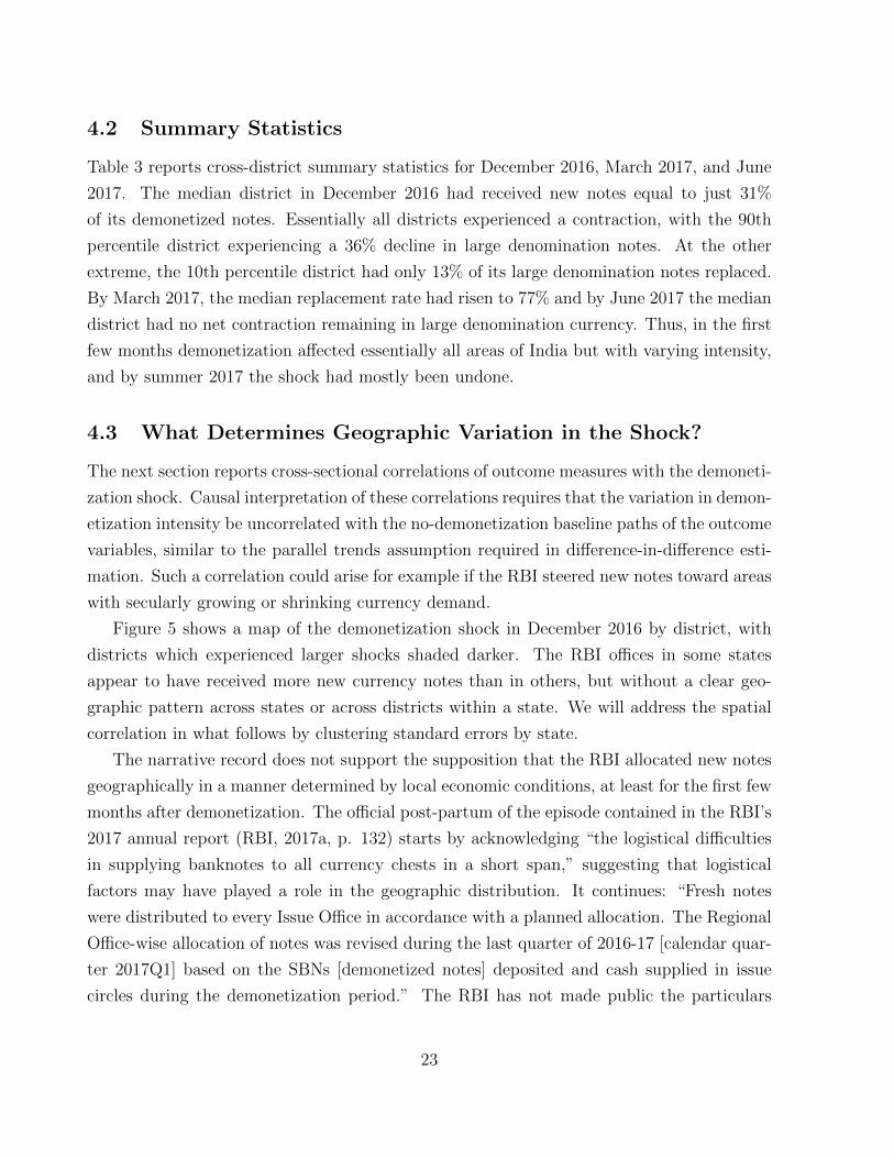
4.2 Summary Statistics

Table 3 reports cross-district summary statistics for December 2016, March 2017, and June

2017. The median district in December 2016 had received new notes equal to just 31%

of its demonetized notes. Essentially all districts experienced a contraction, with the 90th

percentile district experiencing a 36% decline in large denomination notes. At the other

extreme, the 10th percentile district had only 13% of its large denomination notes replaced.

By March 2017, the median replacement rate had risen to 77% and by June 2017 the median

district had no net contraction remaining in large denomination currency. Thus, in the first

few months demonetization affected essentially all areas of India but with varying intensity,

and by summer 2017 the shock had mostly been undone.

4.3 What Determines Geographic Variation in the Shock?

The next section reports cross-sectional correlations of outcome measures with the demoneti-

zation shock. Causal interpretation of these correlations requires that the variation in demon-

etization intensity be uncorrelated with the no-demonetization baseline paths of the outcome

variables, similar to the parallel trends assumption required in difference-in-difference esti-

mation. Such a correlation could arise for example if the RBI steered new notes toward areas

with secularly growing or shrinking currency demand.

Figure 5 shows a map of the demonetization shock in December 2016 by district, with

districts which experienced larger shocks shaded darker. The RBI offices in some states

appear to have received more new currency notes than in others, but without a clear geo-

graphic pattern across states or across districts within a state. We will address the spatial

correlation in what follows by clustering standard errors by state.

The narrative record does not support the supposition that the RBI allocated new notes

geographically in a manner determined by local economic conditions, at least for the first few

months after demonetization. The official post-partum of the episode contained in the RBI’s

2017 annual report (RBI, 2017a, p. 132) starts by acknowledging “the logistical difficulties

in supplying banknotes to all currency chests in a short span,” suggesting that logistical

factors may have played a role in the geographic distribution. It continues: “Fresh notes

were distributed to every Issue Office in accordance with a planned allocation. The Regional

Office-wise allocation of notes was revised during the last quarter of 2016-17 [calendar quar-

ter 2017Q1] based on the SBNs [demonetized notes] deposited and cash supplied in issue

circles during the demonetization period.” The RBI has not made public the particulars

23

Table 3: Summary Statistics

Mean Sd P10 P50 P90 Count2016m12Demonetization shock 0.36 0.24 0.13 0.31 0.64 543Nightlights (log change) −0.08 0.22 −0.33 −0.08 0.16 541ATM transactions (log change) −0.85 0.42 −1.44 −0.77 −0.42 535POS transactions (log change) 2.26 0.83 1.35 2.19 3.31 526E-Wallet transactions (log change) 0.68 0.34 0.34 0.65 1.07 516Bank deposits (log change) 0.12 0.05 0.06 0.12 0.19 536Bank credit (log change) −0.01 0.04 −0.04 −0.01 0.02 5362015 GDP per capita (Mi) 0.10 0.08 0.04 0.09 0.18 5402015 Agriculture share of GDP (%) 16.26 12.43 2.70 13.80 34.50 5322017m3Demonetization shock 0.85 0.44 0.39 0.77 1.36 551Nightlights (log change) 0.18 0.26 −0.09 0.15 0.49 548ATM transactions (log change) 0.01 0.31 −0.19 0.01 0.24 544POS transactions (log change) 1.73 0.95 0.87 1.66 2.76 531E-Wallet transactions (log change) 0.91 0.30 0.54 0.90 1.28 520Bank deposits (log change) 0.13 0.06 0.07 0.12 0.19 544Bank credit (log change) 0.06 0.05 0.02 0.07 0.11 5442015 GDP per capita (Mi) 0.10 0.08 0.04 0.09 0.19 5482015 Agriculture share of GDP (%) 16.17 12.37 2.70 13.70 34.50 5402017m6Demonetization shock 1.19 0.63 0.52 1.07 1.97 549Nightlights (log change) 0.28 0.31 −0.02 0.26 0.67 546ATM transactions (log change) −0.03 0.21 −0.18 −0.04 0.16 542POS transactions (log change) 1.77 0.80 0.98 1.69 2.66 530E-Wallet transactions (log change) 1.14 0.35 0.73 1.16 1.53 518Bank deposits (log change) 0.12 0.05 0.07 0.12 0.18 542Bank credit (log change) 0.08 0.06 0.02 0.08 0.12 5422015 GDP per capita (Mi) 0.10 0.08 0.04 0.09 0.19 5462015 Agriculture share of GDP (%) 16.17 12.34 2.70 13.70 34.50 538

of the “planned allocation,” but its sophistication would have been limited by the secrecy

surrounding the policy prior to its announcement as very few officials even within the gov-

ernment knew of the policy ahead of time. Moreover, the RBI in October 2016 could not

have known the precise geographic distribution of existing 500 and 1000 notes in circulation.

The next sentence of the report indicates that the RBI did not begin to incorporate real-

24

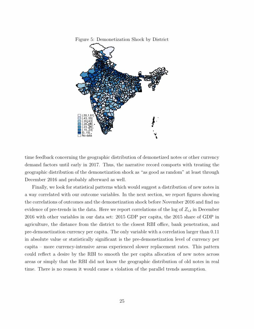
Figure 5: Demonetization Shock by District

(.55,1.81](.43,.55](.35,.43](.28,.35](.23,.28](.15,.23][0,.15]No data

time feedback concerning the geographic distribution of demonetized notes or other currency

demand factors until early in 2017. Thus, the narrative record comports with treating the

geographic distribution of the demonetization shock as “as good as random” at least through

December 2016 and probably afterward as well.

Finally, we look for statistical patterns which would suggest a distribution of new notes in

a way correlated with our outcome variables. In the next section, we report figures showing

the correlations of outcomes and the demonetization shock before November 2016 and find no

evidence of pre-trends in the data. Here we report correlations of the log of Zi,t in December

2016 with other variables in our data set: 2015 GDP per capita, the 2015 share of GDP in

agriculture, the distance from the district to the closest RBI office, bank penetration, and

pre-demonetization currency per capita. The only variable with a correlation larger than 0.11

in absolute value or statistically significant is the pre-demonetization level of currency per

capita – more currency-intensive areas experienced slower replacement rates. This pattern

could reflect a desire by the RBI to smooth the per capita allocation of new notes across

areas or simply that the RBI did not know the geographic distribution of old notes in real

time. There is no reason it would cause a violation of the parallel trends assumption.

25

Table 4: What is the Currency Shock Correlated With?

(1) (2) (3) (4) (5) (6)Log GDP per capita −0.11 0.06

(0.17) (0.27)Agriculture share of GDP −0.04 −0.11

(0.08) (0.10)Log distance to closest RBI office 0.10 0.03

(0.06) (0.07)Log Bank branches per million persons −0.11 −0.09

(0.13) (0.17)Log Pre-demonetization currency per capita −0.27∗∗−0.28∗∗

(0.07) (0.07)BM df 13.0 9.8 19.7 18.8 19.0R2 0.01 0.00 0.01 0.01 0.07 0.08Clusters 31 31 33 31 33 31Observations 538 530 540 535 540 527

Notes: The table reports the correlation coefficient (columns 1-5) and partial correlation coefficient (column6) with zi,t, the log of the currency shock. Standard errors in parentheses clustered by state using the “LZ2”bias-reduction modification suggested by Imbens and Kolesar (2016). The row “BM df” gives the associatedt-distribution degrees of freedom for the coefficient. ∗∗ denotes significance at the 1 percent level.

5 Empirical Findings

In this section we use the geographic variation in the net drop in cash due to demonetization

to document the following results: (i) demonetization caused cash shortages, as evidenced

by a sharper decline in ATM withdrawals in areas with larger shocks; (ii) economic activity,

as measured by employment rates and nightlights, fell in these areas relative to areas which

experienced smaller shocks; (iii) these areas adopted alternative forms of payment; and (iv)

deposits increased more and credit fell in these areas. These results, which come from

disparate data sources and reflect different aspects of demonetization, together provide a

consistent account of the effects of demonetization.

5.1 Aggregate Time Series

Before presenting cross-sectional results, we first plot the aggregate time series in figure 6.

The vertical line in each figure shows the period in which demonetization occurred.

Demonetization has a clear effect on aggregate ATM withdrawals and use of e-wallets

26

and POS payment technologies. These variables exhibit essentially no growth in the periods

before demonetization and then a sharp contraction (ATM withdrawals) or increase (e-wallet

and POS) exactly at the time demonetization occurred. The scale of the changes in these

variables – a 50% decline in ATM withdrawals, a doubling of e-wallet transactions, and

a sextupling of POS transactions between October and December 2016 – seem difficult to

attribute to any economic shock other than demonetization.20

In contrast, the variables representing aggregate real economic activity – GDP growth,

employment, and nightlights – do not exhibit clear patterns around demonetization, nor

do bank deposits or credit.21 Real GDP growth remained in the range 5.6-6.5 percent

(annualized) in the four quarters surrounding demonetization. However, other economic

shocks and policies besides demonetization affected the global economy and India specifically

during this period. Salient examples include the election of Donald Trump which occurred

on the same day as the demonetization announcement, a rise in the global price of crude

oil of 60% from January to October 2016, a better Monsoon rainfall than in the previous

year, increased uncertainty related to capital flows into Foreign Currency Non-Repatriable

accounts and accompanying exchange rate volatility in November 2016, and an overhaul of

the Indian sales tax collection system in the summer of 2017. Moreover, the official GDP

measure misses much of the informal sector which relies heavily on cash and may have been

especially impacted by demonetization. The absence of a clear break in the data and the

existence of other shocks render aggregate trends uninformative for discerning the impact of

demonetization on the real economy. Instead, we turn to cross-sectional differences.

5.2 Cross-sectional Specification

The cross-sectional approach has two crucial advantages relative to the aggregate time series

plotted in figure 6. First, it holds constant other policies or shocks which affected the whole

economy around the period of demonetization. Importantly, even if other policies or shocks

had differential effects across subnational areas, the cross-sectional approach will still uncover

the causal effect of demonetization as long as the demonetization shock is uncorrelated

with these other variables. Second, instead of a single time series with a possible break

in November 2016, the geographic variation in demonetization intensity generates a large

20Because the wallet company provided us the data only in index format, the e-wallet panel of figure 6shows an unweighted average across districts.

21Rural wage inflation (the only high frequency wage series available) and consumer price inflation remainedpositive and showed no discernible change in trend around demonetization. This is consistent with themodel’s assumption of downward wage and therefore price rigidity.

27

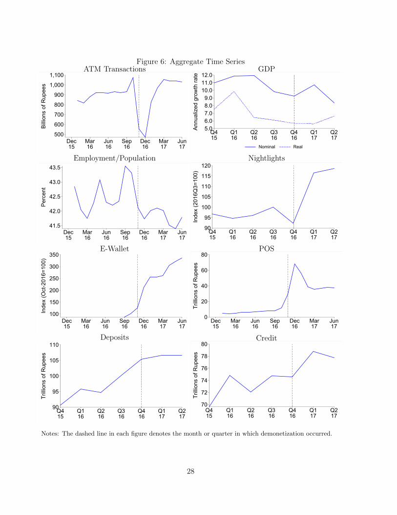
Figure 6: Aggregate Time SeriesATM Transactions

500

600

700

800

900

1,000

1,100

Billio

ns o

f Rup

ees

Dec15

Mar16

Jun16

Sep16

Dec16

Mar17

Jun17

GDP

5.06.07.08.09.0

10.011.012.0

Annu

aliz

ed g

row

th ra

te

Q415

Q116

Q216

Q316

Q416

Q117

Q217

Nominal Real

Employment/Population

41.5

42.0

42.5

43.0

43.5

Perc

ent

Dec15

Mar16

Jun16

Sep16

Dec16

Mar17

Jun17

Nightlights

90

95

100

105

110

115

120

Inde

x (2

016Q

3=10

0)

Q415

Q116

Q216

Q316

Q416

Q117

Q217

E-Wallet

100

150

200

250

300

350

Inde

x (O

ct-2

016=

100)

Dec15

Mar16

Jun16

Sep16

Dec16

Mar17

Jun17

POS

0

20

40

60

80

Trilli

ons

of R

upee

s

Dec15

Mar16

Jun16

Sep16

Dec16

Mar17

Jun17

Deposits

90

95

100

105

110

Trilli

ons

of R

upee

s

Q415

Q116

Q216

Q316

Q416

Q117

Q217

Credit

70

72

74

76

78

80

Trilli

ons

of R

upee

s

Q415

Q116

Q216

Q316

Q416

Q117

Q217

Notes: The dashed line in each figure denotes the month or quarter in which demonetization occurred.

28

sample with varying treatment intensity. The large sample makes possible tighter inference.

Our empirical specification is:

(yi,t − yi,baseline) = β0,t + β1,tzi,treatment + ΓtXi + εi,t, (27)

where yi,t = lnYi,t denotes the natural logarithm of an outcome variable, yi,baseline = lnYi,baseline

denotes the value of the variable in the period immediately preceding demonetization, i.e. Oc-

tober 2016 for monthly frequency data and 2016Q3 for quarterly frequency data, zi,t = lnZi,t

is the log of the demonetization shock, zi,treatment is set to zi,t for t ∈ {November 2016,December 2016}and the December 2016 value for all other periods, and Xi is a vector containing any con-

trols. The coefficients β1,t trace out the cumulative response at various horizons t to the

demonetization shock in December 2016.

We offer three comments on specification (27). First, this specification cannot disentangle

contemporaneous from lagged effects of the demonetization shock in months after December

2016. Rather, the coefficient β1,t reflects both the persistence in zi,t which makes zi,treatment

correlated with zi,t for months after December 2016 and true lagged effects of zi,treatment on

outcomes. We do not attempt to separate these effects because the stability of the rank of

a district in the cross-sectional distribution of shocks yields too little variation to separately

identify contemporaneous from lagged effects.22 Second, some of the dependent variables

used in the analysis have wide tails. The log-log specification helps to reduce sensitivity to

outliers. We further trim observations with dependent variable in the the top and bottom

0.5% of the distribution in the period of analysis. Third, we cluster standard errors by

state to account for the spatial correlation in Zi,t shown in figure 5. This level of clustering

results in about 30 clusters.23 We follow the advice of Imbens and Kolesar (2016) and apply

the “LZ2” correction to the standard errors and compute confidence intervals using a t-

distribution with degrees of freedom suggested by Bell and McCaffrey (2002).24 Imbens and

22For example, the Spearman rank correlation of zi for December 2016 and March 2017 is 0.78.23India consists of 29 states and 7 union territories and we use the term “state” in the main text to

refer to either. We assign districts in Telangana to the same cluster as districts in Andhra Pradesh (theformer was carved out of the latter in 2014 and both states share a single RBI regional office located inHyderabad), have no currency chest data for the territory of Dadra and Nagar Haveli, and exclude theterritory of Chandigarh because it has Zi,t < 0. Therefore, the regressions which follow have a maximum of33 clusters. In specifications controlling for 2015 GDP per capita, we further drop the two union territoriesof Daman & Diu and Lakshadweep due to lack of GDP data.

24The LZ2 correction applies a small sample adjustment which exactly corrects for finite sample bias in thesample counterpart of E[εi,tε

′i,t] when the true sampling distribution of εi,t is i.i.d. The degrees of freedom

for the t-distribution are chosen such that under homoskedasticity the first two moments of the distributionof the error covariance matrix coincide with the first two moments of a chi-squared distribution.

29

Figure 7: ATM Withdrawals

-25.0

-20.0

-15.0

-10.0

-5.0

0.0

Log

chan

ge, O

ct-1

6 to

Dec

-16

-4.0 -3.0 -2.0 -1.0 0.0 1.0Log currency replacement rate

-1.0

0.0

1.0

2.0

3.0

4.0

Reg

ress

ion

coef

ficie

nt

Dec15

Mar16

Jun16

Sep16

Dec16

Mar17

Jun17

Sep17

Notes: The left panel presents a scatter plot of the log change in ATM withdrawals between October 2016and December 2016 and the log currency shock. The light blue circles show the raw data and are sizedproportional to 2015 district GDP. The dark red circles average observations into 50 quantile bins of thecurrency shock. The dashed line gives the best fit line. The right panel reports the coefficient and 95%confidence interval from estimating equation (27) for the period indicated on the horizontal axis.

Kolesar (2016, table 4) present Monte Carlo evidence that the resulting confidence intervals

have good coverage even with as few as five clusters or unbalanced cluster size.

5.3 Results

ATM withdrawals. Figure 7 and table 5 show our first result – areas which received

(proportionally) fewer new notes had sharper declines in ATM activity. The left panel

provides a non-parametric representation of the data. The vertical axis gives the log change

in ATM activity from October 2016, the last full pre-demonetization month, to December

2016, the first full month following demonetization. The horizontal axis shows zi,t, the

log of the average daily value in December 2016 of the demonetization measure described

by equation (26). Each blue circle corresponds to a district, with the size of the circle

proportional to 2015 district GDP. The red circles show the (unweighted) means of the

change in ATM activity for each of 50 quantile bins of zi,t. Thus, the figure overlays a so-

called “binned scatter plot” on top of the raw data. The dashed red line shows the best fit

line.

The right panel of figure 7 reports the coefficient from estimating equation (27) with no

covariates in Xi for each month from November 2015 to June 2017. Thus, the value for

December 2016 gives the slope of the best fit line in the figure in the left panel. The dashed

lines show the (point-wise) 95% confidence intervals.

30

Table 5: ATM Withdrawals

(1) (2) (3)Currency replacement 2.29∗∗ 2.28∗ 2.18∗

(0.66) (0.75) (0.76)Log GDP per capita −0.18 −0.10

(0.80) (0.72)Agriculture share of GDP 0.02 −0.01

(0.03) (0.03)Control lagged outcomes No Yes YesWeight No No YesFitted 90-10 differential 36.5 36.4 34.7Treatment BM df 10.7 11.3 12.5R2 0.14 0.17 0.16Clusters 33 31 31Observations 529 519 519

Notes: The dependent variable is the log point change from October 2016 to December 2016 multiplied by10. Columns (2) and (3) additionally controls for 9 lags of the dependent variable. Column (3) weights theregression by district GDP. Standard errors in parentheses clustered by state using the “LZ2” bias-reductionmodification suggested by Imbens and Kolesar (2016). ∗∗,∗ ,+ denote significance at the 1, 5, or 10 percentlevel based on a t-distribution with degrees of freedom for the currency replacement variable shown in therow “Treatment BM df”.

The figure shows a statistically strong, positive correlation between the arrival of new

currency by December 2016 and ATM withdrawals. The link between money supply and cash

withdrawals validates the usefulness of our geographic shock measure and provides prima

facie evidence of a cash shortfall in which households are off their money demand curve. The

near-zero values in the right panel for months before November 2016 indicate that districts

which experienced larger demonetization shocks exhibited parallel trend growth of ATM

withdrawals before the shock occurred. The cross-sectional impact of the shock on ATM

withdrawals is concentrated in December 2016 but remains through June 2017. In terms of

magnitude, the predicted difference in ATM withdrawals between districts at the 10th and

90th percentiles of the December 2016 shock distribution is 37 log points.

Table 5 demonstrates the robustness of the cross-sectional pattern. Column (1) repro-

duces the slope coefficient from the left panel of figure 7. Column (2) adds covariates to

the regression: 2015 GDP per capita, the 2015 agriculture share of GDP, and nine lags of

ATM transactions growth. The lags of ATM growth control directly for any pre-trends while

the 2015 level of GDP per capita and agriculture share of GDP control for basic features of

the industrial structure of Indian districts. Inclusion of these covariates has little effect on

31

the coefficient on zi,t, consistent with the absence of correlation of zi,t with other variables

shown in table 4. Column (3) weights the regression by district GDP. The coefficient changes

little.25

Employment and nightlights. Figure 8 and table 6 display our next main result –

demonetization reduced real economic activity. The scatter plots in the left panels of figure 8

show non-parametrically that areas with larger declines in currency experienced sharper

declines in employment and in nightlight activity after demonetization occurred. The right

panels show no evidence of pre-trends and highly statistically significant post-demonetization

differences which last into the spring of 2017 before fully dissipating.26

The magnitude of the effect on real activity is substantial. The predicted difference in

employment growth between districts at the 10th and 90th percentiles immediately after

demonetization is 4.6 log points while the predicted difference in nightlight growth is 14.3

log points.27 Based on both annual and long-term growth rate comparisons for a sample

of 188 countries, Henderson, Storeygard, and Weil (2012) argue for an elasticity of GDP

growth to nightlight growth of 0.3. Their estimate remains similar even for a sub-sample of

low and middle-income countries. Using this elasticity yields a predicted difference in GDP

of roughly 4.4 log points. It bears emphasizing that these two measures of economic activity

come from very different sources – a household survey of employment status and satellite

measures of nightlight activity – yet they suggest quantitatively similar declines in output.

The two measures together therefore provide powerful evidence of a link between money and

output during demonetization.

25Weighting would be appropriate if larger districts had less measurement error or if the effect of a givenamount of demonetization varied with district size. The stability of the standard error in the weightedspecification militates against the efficiency rationale. The small change in the point estimate suggests thatweighting due to heterogeneous treatment effects is unnecessary.

26Recall that the employment survey uses a rotation schedule such that each month contains data for onlyabout 150 districts. For this reason, the top left panel of table 6 pools observations from December 2016,January 2017, and February 2017 in order to obtain a more complete sample of districts and the top rightpanel shows coefficients grouping months with the same sample units. Because the data start in January2016, the first point shown in the top right panel contains data from two rather than three months, explainingthe wider confidence interval around that point.

27Technically, the predicted difference in the growth rate of the employment-to-population ratio is 4.6 logpoints. Recall that the household survey data from which we calculate the employment-to-population ratio donot permit measurement of the change in population. Assuming zero effect of demonetization on population,the predicted difference in the growth rate of the employment-to-population ratio is also the predicteddifference in the growth rate of employment. We believe such an assumption to be reasonable given theshort time horizon over which demonetization occurred. Nonetheless, if in fact more severe demonetizationin an area led to worker outflows, then the effect on employment would be larger than the 4.6 log pointdifference given in the main text.

32

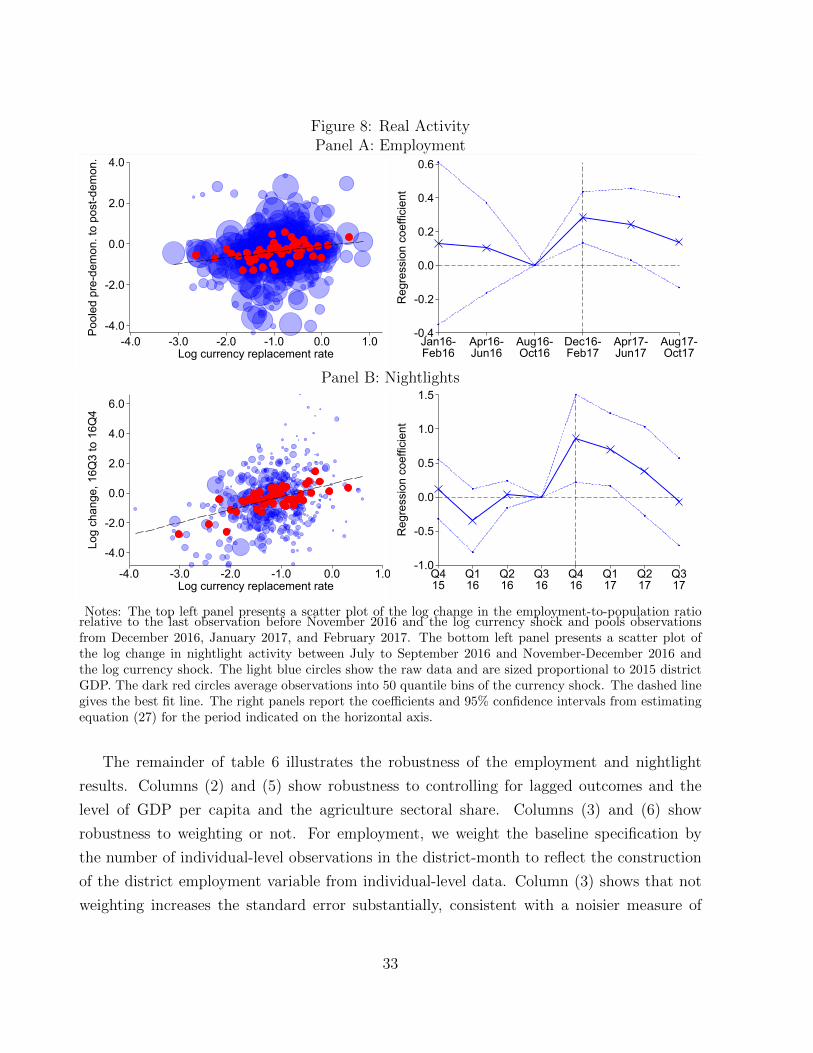
Figure 8: Real ActivityPanel A: Employment

-4.0

-2.0

0.0

2.0

4.0

Pool

ed p

re-d

emon

. to

post

-dem

on.

-4.0 -3.0 -2.0 -1.0 0.0 1.0Log currency replacement rate

-0.4

-0.2

0.0

0.2

0.4

0.6

Reg

ress

ion

coef

ficie

nt

Jan16-Feb16

Apr16-Jun16

Aug16-Oct16

Dec16-Feb17

Apr17-Jun17

Aug17-Oct17

Panel B: Nightlights

-4.0

-2.0

0.0

2.0

4.0

6.0

Log

chan

ge, 1

6Q3

to 1

6Q4

-4.0 -3.0 -2.0 -1.0 0.0 1.0Log currency replacement rate

-1.0

-0.5

0.0

0.5

1.0

1.5R

egre

ssio

n co

effic

ient

Q415

Q116

Q216

Q316

Q416

Q117

Q217

Q317

Notes: The top left panel presents a scatter plot of the log change in the employment-to-population ratiorelative to the last observation before November 2016 and the log currency shock and pools observationsfrom December 2016, January 2017, and February 2017. The bottom left panel presents a scatter plot ofthe log change in nightlight activity between July to September 2016 and November-December 2016 andthe log currency shock. The light blue circles show the raw data and are sized proportional to 2015 districtGDP. The dark red circles average observations into 50 quantile bins of the currency shock. The dashed linegives the best fit line. The right panels report the coefficients and 95% confidence intervals from estimatingequation (27) for the period indicated on the horizontal axis.

The remainder of table 6 illustrates the robustness of the employment and nightlight

results. Columns (2) and (5) show robustness to controlling for lagged outcomes and the

level of GDP per capita and the agriculture sectoral share. Columns (3) and (6) show

robustness to weighting or not. For employment, we weight the baseline specification by

the number of individual-level observations in the district-month to reflect the construction

of the district employment variable from individual-level data. Column (3) shows that not

weighting increases the standard error substantially, consistent with a noisier measure of

33

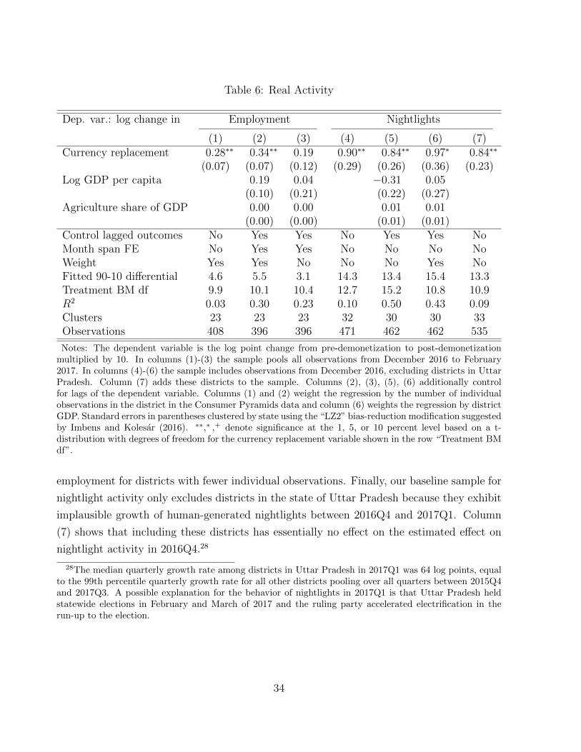
Table 6: Real Activity

Dep. var.: log change in Employment Nightlights

(1) (2) (3) (4) (5) (6) (7)Currency replacement 0.28∗∗ 0.34∗∗ 0.19 0.90∗∗ 0.84∗∗ 0.97∗ 0.84∗∗

(0.07) (0.07) (0.12) (0.29) (0.26) (0.36) (0.23)Log GDP per capita 0.19 0.04 −0.31 0.05

(0.10) (0.21) (0.22) (0.27)Agriculture share of GDP 0.00 0.00 0.01 0.01

(0.00) (0.00) (0.01) (0.01)Control lagged outcomes No Yes Yes No Yes Yes NoMonth span FE No Yes Yes No No No NoWeight Yes Yes No No No Yes NoFitted 90-10 differential 4.6 5.5 3.1 14.3 13.4 15.4 13.3Treatment BM df 9.9 10.1 10.4 12.7 15.2 10.8 10.9R2 0.03 0.30 0.23 0.10 0.50 0.43 0.09Clusters 23 23 23 32 30 30 33Observations 408 396 396 471 462 462 535

Notes: The dependent variable is the log point change from pre-demonetization to post-demonetizationmultiplied by 10. In columns (1)-(3) the sample pools all observations from December 2016 to February2017. In columns (4)-(6) the sample includes observations from December 2016, excluding districts in UttarPradesh. Column (7) adds these districts to the sample. Columns (2), (3), (5), (6) additionally controlfor lags of the dependent variable. Columns (1) and (2) weight the regression by the number of individualobservations in the district in the Consumer Pyramids data and column (6) weights the regression by districtGDP. Standard errors in parentheses clustered by state using the “LZ2” bias-reduction modification suggestedby Imbens and Kolesar (2016). ∗∗,∗ ,+ denote significance at the 1, 5, or 10 percent level based on a t-distribution with degrees of freedom for the currency replacement variable shown in the row “Treatment BMdf”.

employment for districts with fewer individual observations. Finally, our baseline sample for

nightlight activity only excludes districts in the state of Uttar Pradesh because they exhibit

implausible growth of human-generated nightlights between 2016Q4 and 2017Q1. Column

(7) shows that including these districts has essentially no effect on the estimated effect on

nightlight activity in 2016Q4.28

28The median quarterly growth rate among districts in Uttar Pradesh in 2017Q1 was 64 log points, equalto the 99th percentile quarterly growth rate for all other districts pooling over all quarters between 2015Q4and 2017Q3. A possible explanation for the behavior of nightlights in 2017Q1 is that Uttar Pradesh heldstatewide elections in February and March of 2017 and the ruling party accelerated electrification in therun-up to the election.

34

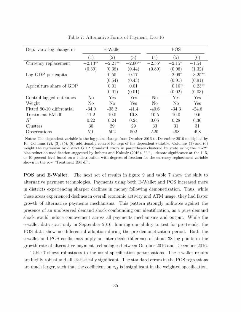
Table 7: Alternative Forms of Payment, Dec-16

Dep. var.: log change in E-Wallet POS

(1) (2) (3) (4) (5) (6)Currency replacement −2.13∗∗ −2.21∗∗ −2.60∗∗ −2.55∗ −2.15∗ −1.54

(0.39) (0.38) (0.44) (0.89) (0.96) (1.32)Log GDP per capita −0.55 −0.17 −2.09∗ −3.25∗∗

(0.54) (0.43) (0.91) (0.91)Agriculture share of GDP 0.01 0.01 0.16∗∗ 0.23∗∗

(0.01) (0.01) (0.02) (0.03)Control lagged outcomes No Yes Yes No Yes YesWeight No No Yes No No YesFitted 90-10 differential -34.0 -35.2 -41.4 -40.6 -34.3 -24.6Treatment BM df 11.2 10.5 10.8 10.5 10.0 9.6R2 0.22 0.24 0.24 0.05 0.28 0.36Clusters 30 29 29 33 31 31Observations 510 502 502 520 498 498

Notes: The dependent variable is the log point change from October 2016 to December 2016 multiplied by10. Columns (2), (3), (5), (6) additionally control for lags of the dependent variable. Columns (3) and (6)weight the regression by district GDP. Standard errors in parentheses clustered by state using the “LZ2”bias-reduction modification suggested by Imbens and Kolesar (2016). ∗∗,∗ ,+ denote significance at the 1, 5,or 10 percent level based on a t-distribution with degrees of freedom for the currency replacement variableshown in the row “Treatment BM df”.

POS and E-Wallet. The next set of results in figure 9 and table 7 show the shift to

alternative payment technologies. Payments using both E-Wallet and POS increased more

in districts experiencing sharper declines in money following demonetization. Thus, while

these areas experienced declines in overall economic activity and ATM usage, they had faster

growth of alternative payments mechanisms. This pattern strongly militates against the

presence of an unobserved demand shock confounding our identification, as a pure demand

shock would induce comovement across all payments mechanisms and output. While the

e-wallet data start only in September 2016, limiting our ability to test for pre-trends, the

POS data show no differential adoption during the pre-demonetization period. Both the

e-wallet and POS coefficients imply an inter-decile difference of about 38 log points in the

growth rate of alternative payment technologies between October 2016 and December 2016.

Table 7 shows robustness to the usual specification perturbations. The e-wallet results

are highly robust and all statistically significant. The standard errors in the POS regressions

are much larger, such that the coefficient on zi,t is insignificant in the weighted specification.

35

Figure 9: Alternative Forms of PaymentPanel A: E-Wallet

0.0

5.0

10.0

15.0

20.0

Log

chan

ge, O

ct-1

6 to

Dec

-16

-4.0 -3.0 -2.0 -1.0 0.0 1.0Log currency replacement rate

-3.0

-2.0

-1.0

0.0

1.0

Reg

ress

ion

coef

ficie

nt

Dec15

Mar16

Jun16

Sep16

Dec16

Mar17

Jun17

Sep17

Panel B: POS

-10.0

0.0

10.0

20.0

30.0

40.0

50.0

Log

chan

ge, O

ct-1

6 to

Dec

-16

-4.0 -3.0 -2.0 -1.0 0.0 1.0Log currency replacement rate

-4.0

-2.0

0.0

2.0

4.0R

egre

ssio

n co

effic

ient

Dec15

Mar16

Jun16

Sep16

Dec16

Mar17

Jun17

Sep17

Notes: The left panels present scatter plots of the log change in e-wallet transactions (top row) or POStransactions (bottom row) between October 2016 and December 2016 and the log currency shock. The lightblue circles show the raw data and are sized proportional to 2015 district GDP. The dark red circles averageobservations into 50 quantile bins of the currency shock. The dashed line gives the best fit line. The rightpanels report the coefficients and 95% confidence intervals from estimating equation (27) for the periodindicated on the horizontal axis.

Deposits and Credit. Figure 10 and table 8 report our final set of results covering bank

deposit and credit growth. We find evidence of bank deposits increasing and credit con-

tracting in areas experiencing more severe demonetization. The effect on deposits appears

short-lived while the effect on credit may be more persistent. Because banks have access to

internal credit markets and banks in more-demonetized districts experienced faster deposit

growth, we can interpret the contraction in lending in those districts as due to lower borrower

demand for credit. As a caveat to these results, recall that the credit variable corresponds

to loans made by banks within a district regardless of the location of the borrower. These

results appear broadly robust to alternative specifications.

36

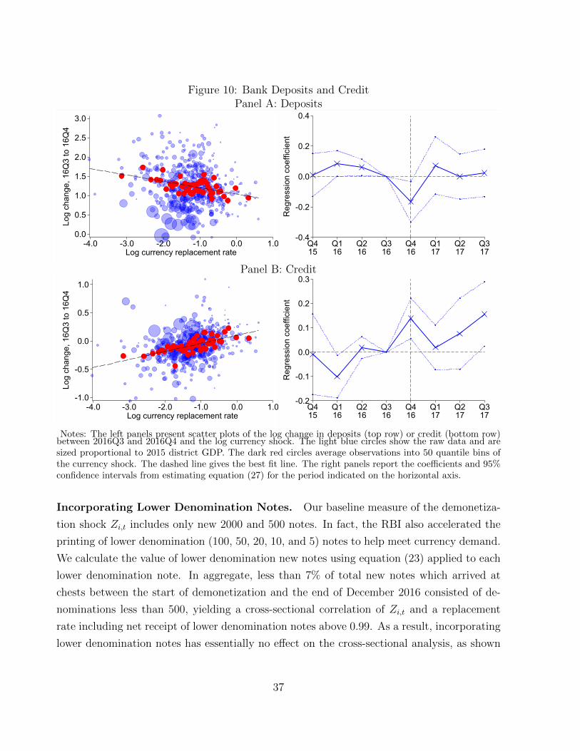
Figure 10: Bank Deposits and CreditPanel A: Deposits

0.0

0.5

1.0

1.5

2.0

2.5

3.0

Log

chan

ge, 1

6Q3

to 1

6Q4

-4.0 -3.0 -2.0 -1.0 0.0 1.0Log currency replacement rate

-0.4

-0.2

0.0

0.2

0.4

Reg

ress

ion

coef

ficie

nt

Q415

Q116

Q216

Q316

Q416

Q117

Q217

Q317

Panel B: Credit

-1.0

-0.5

0.0

0.5

1.0

Log

chan

ge, 1

6Q3

to 1

6Q4

-4.0 -3.0 -2.0 -1.0 0.0 1.0Log currency replacement rate

-0.2

-0.1

0.0

0.1

0.2

0.3R

egre

ssio

n co

effic

ient

Q415

Q116

Q216

Q316

Q416

Q117

Q217

Q317

Notes: The left panels present scatter plots of the log change in deposits (top row) or credit (bottom row)between 2016Q3 and 2016Q4 and the log currency shock. The light blue circles show the raw data and aresized proportional to 2015 district GDP. The dark red circles average observations into 50 quantile bins ofthe currency shock. The dashed line gives the best fit line. The right panels report the coefficients and 95%confidence intervals from estimating equation (27) for the period indicated on the horizontal axis.

Incorporating Lower Denomination Notes. Our baseline measure of the demonetiza-

tion shock Zi,t includes only new 2000 and 500 notes. In fact, the RBI also accelerated the

printing of lower denomination (100, 50, 20, 10, and 5) notes to help meet currency demand.

We calculate the value of lower denomination new notes using equation (23) applied to each

lower denomination note. In aggregate, less than 7% of total new notes which arrived at

chests between the start of demonetization and the end of December 2016 consisted of de-

nominations less than 500, yielding a cross-sectional correlation of Zi,t and a replacement

rate including net receipt of lower denomination notes above 0.99. As a result, incorporating

lower denomination notes has essentially no effect on the cross-sectional analysis, as shown

37

Table 8: Bank Deposits and Credit, 2016Q4

Dep. var.: log change in Deposits Credit

(1) (2) (3) (4) (5) (6)Currency replacement −0.17∗ −0.18∗∗ −0.14 0.14∗∗ 0.12∗∗ 0.06+

(0.06) (0.06) (0.09) (0.04) (0.03) (0.03)Log GDP per capita −0.20∗∗ −0.27∗∗ 0.00 0.06

(0.06) (0.07) (0.02) (0.04)Agriculture share of GDP 0.01∗∗ 0.02∗∗ −0.00∗ −0.00∗

(0.00) (0.00) (0.00) (0.00)Control lagged outcomes No Yes Yes No Yes YesWeight No No Yes No No YesFitted 90-10 differential -2.7 -2.8 -2.2 2.2 2.0 1.0Treatment BM df 11.1 9.8 10.2 11.3 11.8 11.4R2 0.05 0.24 0.37 0.10 0.21 0.24Clusters 32 30 30 32 30 30Observations 529 520 520 529 519 519

Notes: The dependent variable is the log point change from 2016Q3 to 2016Q4 multiplied by 10. Columns(2), (3), (5), (6) additionally control for lags of the dependent variable. Columns (3) and (6) weight theregression by district GDP. Standard errors in parentheses clustered by state using the “LZ2” bias-reductionmodification suggested by Imbens and Kolesar (2016). ∗∗,∗ ,+ denote significance at the 1, 5, or 10 percentlevel based on a t-distribution with degrees of freedom for the currency replacement variable shown in therow “Treatment BM df”.

formally in table 9.

6 Discussion and Relation to Aggregate Effect

The cross-sectional results establish that areas experiencing more severe demonetization

had sharper declines in ATM withdrawals, reduced economic activity, faster adoption of

alternative payment technologies, and higher deposit and lower bank credit growth. Among

these results, the effect on real economic activity stands out in its contrast to the aggregate

GDP time series. We now explore this difference in greater detail and what the cross-sectional

evidence implies for the effect of demonetization on aggregate economic activity.

We start by cumulating the cross-sectional effects over districts. This calculation involves

using the cross-sectional coefficient to impute to each district the change in the outcome

variable relative to if no change in money balances had occurred, i.e. Zi,t = 1, and then

38

Table 9: Cross-sectional Elasticities Including Lower Denomination Notes

Dep. var. Baseline Including lower denomination notes

β1,t s.e. β1,t s.e.ATM withdrawals 2.29∗∗ 0.66 2.35∗∗ 0.62Employment 0.28∗∗ 0.07 0.28∗∗ 0.07Nightlights 0.90∗∗ 0.29 0.85∗∗ 0.29E-Wallet −2.13∗∗ 0.39 −2.05∗∗ 0.41POS −2.55∗ 0.89 −2.52∗ 0.91Deposits −0.17∗ 0.06 −0.15∗ 0.07Bank credit 0.14∗∗ 0.04 0.13∗∗ 0.04

Notes: The left panel reproduces the coefficients without controls in tables 5 to 8. The right panel reportsthe corresponding coefficients based on a measure of the demonetization shock zi,t which includes receiptof all denominations of notes in the numerator. Standard errors clustered by state using the “LZ2” bias-reduction modification suggested by Imbens and Kolesar (2016). ∗∗,∗ ,+ denote significance at the 1, 5, or 10percent level based on a t-distribution with degrees of freedom for the currency replacement variable shownin the row “Treatment BM df”.

summing over districts. The formula for the cumulated effect in month t is:∑i:Zi,t≤1

(eβ1,tzi,t − 1

)Yi,baseline∑

i Yi,baseline≈β1,t

∑i:Zi,t≤1 zi,tYi,baseline∑

i Yi,baseline. (28)

Using the coefficients show in columns (1) and (4) of table 6, for employment this calculation

yields a decline of 3.7 p.p., while for nightlights this calculation yields a decline of 11.7 p.p.

which translates into an output decline of 3.5 p.p. after applying the 0.3 elasticity advocated

by Henderson, Storeygard, and Weil (2012).

Importantly, the preceding calculation assumes a log-linear relationship between the cash

shortage and outcome variables. While the scatter plots shown above appear consistent

with such linearity, because essentially all districts experienced a large decline in currency

we lack the power to test for a non-linearity or kink at small declines in cash. Nonetheless,

assuming instead a flat relationship (no effect of the cash shortage on outcomes) above a 0.9

replacement rate would only change the implied decline in employment to 3.3 p.p. and the

decline in nightlights to 10.8 p.p. Similarly, accounting for the introduction of new lower

denomination notes would raise the replacement rate and hence lower the cumulated cross-

sectional shortfall by about 7%, yielding for example an implied decline in employment of

0.93× 3.7 = 3.4p.p.

The next step is to relate the cumulated quantity defined in equation (28) to the ac-

39

tual national effect. To do so we return to the model of section 3. There, the cumulated

decline in output provides a lower bound for the true aggregate decline. The lower bound

arises because of the tradeables sector; some of the demand shortfall in a local area gets ex-

ported to other areas through trade linkages. This logic closely relates to theoretical results

presented in Nakamura and Steinsson (2014), Farhi and Werning (2016), and Chodorow-

Reich (Forthcoming) in the context of estimation of cross-sectional fiscal multipliers. In the

demonetization context the lower bound is especially sharp because national interest rates

remained fixed and total government liabilities did not change.

Applying the lower bound result to the cross-sectional estimates for employment and

nightlights, we conclude that demonetization caused a decline in national economic activity

of roughly 3 p.p. or more in November and December 2016 relative to a no-demonetization

counterfactual.29 Similarly, the effect on credit implies a 2 p.p. or more decline in 2016Q4.

These effects dissipate over the few months.

Is such a decline large? The magnitude of the peak effect on output makes demonetization

comparable to a roughly 200 basis point tightening of the monetary policy rate based on

the median of estimates reviewed in Ramey (2016) of econometric studies of U.S. data.

Moreover, it implies a rejection of the cashless limit wherein all that matters in the conduct

of monetary policy is the interest rate. On the other hand, the output decline is an order of

magnitude smaller than the decline in cash itself. This difference illustrates the Lucas (1976)

critique in action – in response to a change in policy, agents endogenously adjust (changing

κ in our model) rather than passively obeying a pre-existing CIA constraint.

Why does the decline in output not obviously materialize in the national GDP data? As

already mentioned, national data are volatile and subject to other shocks, making it difficult

to discern a single break point around demonetization. Moreover, our measures of real activ-

ity have the advantage over official GDP of directly incorporating informal sector activity.

The informal sector in India is estimated to account for 81% of total employment (ILO,

2018) and 44% of total output (CSO, 2018) and is especially cash-intensive. While the level

of official GDP includes an estimate of informal sector activity derived from a quinquennial

household survey, quarterly changes in GDP do not reflect any direct measurement of infor-

mal sector activity. Thus, our results also point to the likelihood of an absolute decline in

29The aggregated changes in ATM withdrawals, e-wallet transactions, and POS transactions from applyingequation (28) are also all smaller than the actual aggregate changes. However, some special factors apply tothese variables. Many ATMs temporarily went out of service to receive recalibration required to dispense thenew notes, independent of cash availability. Increasing returns to scale of payments technologies, informationnetwork effects, and increased advertising all may have contributed to a common component of adoption ofalternative payments technologies across areas.

40

economic activity at the end of 2016 not captured in official statistics.30

In conclusion, we emphasize that we focus in this paper on the near term impact of

demonetization. Our identification strategy based on random shocks to the cross-section

of districts best lends itself to near term analysis because these cross-sectional differences

dissipate in the months following demonetization. There may be longer term advantages from

demonetization that arise from improvements in tax collections and in a shift to savings

in financial instruments and non-cash payment mechanisms. Evaluating these long-term

consequences requires waiting for more data and an empirical strategy suited to the study

of longer term effects.

30In the context of our model, aggregate economic activity must have declined if the wage constraint wasbinding. If trend growth in India was 1.5% per quarter (6% per year), then our estimates imply an absolutedecline in economic activity of about 0.5% in 2016Q4 from the previous quarter. This follows from the 3%decline in November and December and no impact in the pre-demonetization month of October.

41

References

Aggarwal, N., and S. Narayanan (2017): “Impact of India’s Demonetization on Do-

mestic Agricultural Markets,” .

Agrawal, S. (2018): “Black Economy and Demonetisation,” .

Alvarez, F., and F. Lippi (2009): “Financial Innovation and the Transactions Demand

for Cash,” Econometrica, 77(2), 363–402.

Banerjee, A., E. Breza, A. G. Chandrasekhar, and B. Golub (2018): “When Less

is More: Experimental Evidence on Information Delivery During India’s Demonetization,”

Working Paper 24679, National Bureau of Economic Research.

Banerjee, A., and N. Kala (2017): “The Economic and Political Consequences of India’s

Demonetization,” .

Bell, R., and D. McCaffrey (2002): “Bias Reduction in Standard Errors for Linear

Regression with Multi-Stage Samples,” Survey Methodology, 28, 169–181.

Chodorow-Reich, G. (Forthcoming): “Geographic Cross-Sectional Fiscal Multipliers:

What Have We Learned?,” American Economic Journal: Economic Policy.

Crouzet, N., A. Gupta, and F. Mezzanotti (2018): “Shocks and Technology Adop-

tion: Evidence from Electronic Payment Systems,” Working paper.

CSO (2018): “First Revised Estimates Of National Income, Consumption Expenditure,

Saving And Capital Formation For 2016-17,” Discussion paper, Central Statistics Office,

Government of India.

Elvidge, C., K. Baugh, M. Zhizhin, F. Hsu, and T. Ghosh (2017): “VIIRS Night-

time Lights,” International Journal of Remote Sensing, 38(21), 5860–5879.

Farhi, E., and I. Werning (2016): “Fiscal Multipliers: Liquidity Traps and Currency

Unions,” in Handbook of Macroeconomics. Harvard University mimeo.

Henderson, J. V., A. Storeygard, and D. N. Weil (2012): “Measuring Economic

Growth from Outer Space,” American Economic Review, 102(2), 994–1028.

ILO (2018): “Women and Men in the Informal Economy: A Statistical Picture,” Discussion

paper, International Labour Office.

42

Imbens, G. W., and M. Kolesar (2016): “Robust Standard Errors in Small Samples:

Some Practical Advice,” The Review of Economics and Statistics, 98(4), 701–712.

Kaur, Supreet (forthcoming): “Nominal Wage Rigidity in Village Labor Markets,” Amer-

ican Economic Review.

Kocherlakota, N. R. (1998): “Money Is Memory,” Journal of Economic Theory, 81(2),

232 – 251.

Krishnan, D., and S. Siegel (2017): “Survey of the Effects of Demonetisation on 28

Slum Neighborhoods of Mumbai,” Economic & Political Weekly, 52(3).

Lagos, R., and S. Zhang (2018): “On Money as a Medium of Exchange in Near-Cashless

Credit Economies,” Working paper.

Lucas, R. E. (1976): “Econometric policy evaluation: A critique,” Carnegie-Rochester

Conference Series on Public Policy, 1, 19 – 46.

(1982): “Interest rates and currency prices in a two-country world,” Journal of

Monetary Economics, 10(3), 335 – 359.

Lucas, R. E., and N. L. Stokey (1987): “Money and Interest in a Cash-in-Advance

Economy,” Econometrica, 55(3), 491–513.

Nakamura, E., and J. Steinsson (2014): “Fiscal Stimulus in a Monetary Union: Evi-

dence from US Regions,” American Economic Review, 104(3), 753–92.

Nakamura, E., and J. Steinsson (2018): “Identification in Macroeconomics,” Journal

of Economic Perspectives, 32(3), 59–86.

Ramey, V. (2016): “Chapter 2 - Macroeconomic Shocks and Their Propagation,” vol. 2 of

Handbook of Macroeconomics, pp. 71 – 162. Elsevier.

RBI (2017a): “Annual Report 2016-17,” Discussion paper, Reserve Bank of India.

(2017b): “Macroeconomic Impact of Demonetisation – A Preliminary Assessment,”

Discussion paper, Reserve Bank of India.

(2018): “Annual Report 2017-18,” Discussion paper, Reserve Bank of India.

Rogoff, K. S. (2016): The Curse of Cash: How Large-Denomination Bills Aid Crime and

Tax Evasion and Constrain Monetary Policy. Princeton University Press.

43

Schmitt-Grohe, S., and M. Uribe (2016): “Downward Nominal Wage Rigidity, Cur-

rency Pegs, and Involuntary Unemployment,” Journal of Political Economy, 124(5), 1466–

1514.

Svensson, L. E. O. (1985): “Money and Asset Prices in a Cash-in-Advance Economy,”

Journal of Political Economy, 93(5), 919–944.

Velde, F. R. (2009): “Chronicle of a Deflation Unforetold,” Journal of Political Economy,

117(4), 591–634.

Williamson, S., and R. Wright (2010): “New Monetarist Economics: Methods,” Re-

search Department Staff Report 442, Federal Reserve Bank of Minneapolis.

Woodford, M. (2003): Interest and Prices: Foundations of a Theory of Monetary Policy.

Princeton University Press.

World Bank (2017): “Growth Out of The Blue,” South Asia Economic Focus.

44

Cash and the Economy:

Evidence from India’s Demonetization

Online Appendix

Gabriel Chodorow-Reich Gita Gopinath

Prachi Mishra Abhinav Narayanan

A Model Proofs

Proof of proposition 1

Begin by assuming θ−1 = 0, we will later derive the parameter restrictions under which this

is the case. From the F.O.C. for cash in the steady state, we have that:

η−1 =1

νlog

(ντ

1− β

)From the definition of η it the follows that:

W−1 =M−1

N−1η−1

From the F.O.C. for consumption in a zero inflation steady state it follows that real

consumption is constant which implies that labor is constant. This further implies that

wages are constant so the downward nominal rigidity is not binding and the economy is in

full employment, i.e. N−1 = N

Now, again using the definition of η−1 and the firms optimality conditions we have:

W−1 =M−1

Nη−1

, P T−1 = PN

−1 = (1 + ϕ(β−1 − 1))M−1

Nη−1

As prices for both types of goods are the same, using the F.O.C. for tradable and non-

tradable goods we have that:

CN−1

CT−1

=1− αα

1

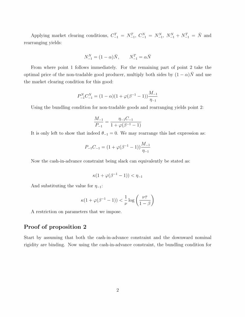
Applying market clearing conditions, CT−1 = NT

−1, CN−1 = NN

−1, NN−1 + NT

−1 = N and

rearranging yields:

NN−1 = (1− α)N , NT

−1 = αN

From where point 1 follows immediately. For the remaining part of point 2 take the

optimal price of the non-tradable good producer, multiply both sides by (1 − α)N and use

the market clearing condition for this good:

PN−1C

N−1 = (1− α)(1 + ϕ(β−1 − 1))

M−1

η−1

Using the bundling condition for non-tradable goods and rearranging yields point 2:

M−1

P−1

=η−1C−1

1 + ϕ(β−1 − 1)

It is only left to show that indeed θ−1 = 0. We may rearrange this last expression as:

P−1C−1 = (1 + ϕ(β−1 − 1))M−1

η−1

Now the cash-in-advance constraint being slack can equivalently be stated as:

κ(1 + ϕ(β−1 − 1)) < η−1

And substituting the value for η−1:

κ(1 + ϕ(β−1 − 1)) <1

νlog

(ντ

1− β

)A restriction on parameters that we impose.

Proof of proposition 2

Start by assuming that both the cash-in-advance constraint and the downward nominal

rigidity are binding. Now using the cash-in-advance constraint, the bundling condition for

2

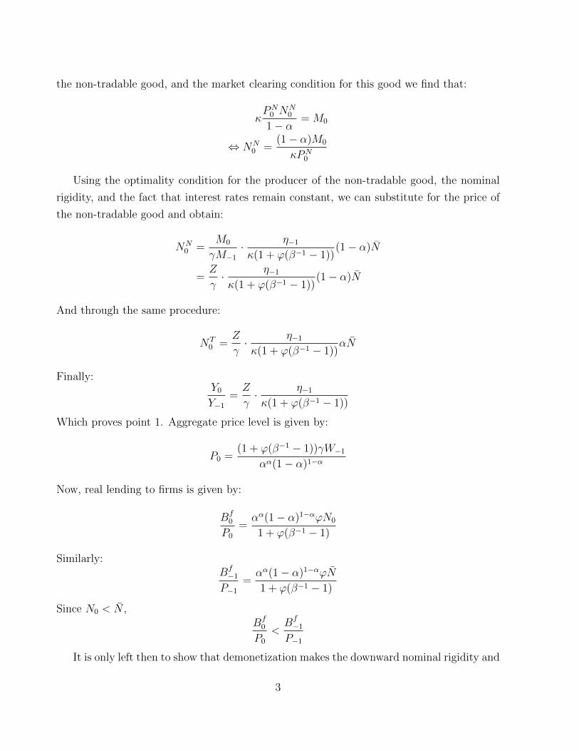
the non-tradable good, and the market clearing condition for this good we find that:

κPN

0 NN0

1− α= M0

⇔ NN0 =

(1− α)M0

κPN0

Using the optimality condition for the producer of the non-tradable good, the nominal

rigidity, and the fact that interest rates remain constant, we can substitute for the price of

the non-tradable good and obtain:

NN0 =

M0

γM−1

· η−1

κ(1 + ϕ(β−1 − 1))(1− α)N

=Z

γ· η−1

κ(1 + ϕ(β−1 − 1))(1− α)N

And through the same procedure:

NT0 =

Z

γ· η−1

κ(1 + ϕ(β−1 − 1))αN

Finally:Y0

Y−1

=Z

γ· η−1

κ(1 + ϕ(β−1 − 1))

Which proves point 1. Aggregate price level is given by:

P0 =(1 + ϕ(β−1 − 1))γW−1

αα(1− α)1−α

Now, real lending to firms is given by:

Bf0

P0

=αα(1− α)1−αϕN0

1 + ϕ(β−1 − 1)

Similarly:Bf−1

P−1

=αα(1− α)1−αϕN

1 + ϕ(β−1 − 1)

Since N0 < N ,Bf

0

P0

<Bf−1

P−1

It is only left then to show that demonetization makes the downward nominal rigidity and

3

the cash-in-advance constraint binding. Multiplying both sides of the optimality condition

of non-tradable goods producer by CNi,0 = NN

0 yields:

PN0 C

N0 = (1 + ϕ(β−1 − 1))NN

0 WN0

. Now, using the cash-in-advance constraint and the bundling condition for non-tradable

goods we find that:

(1− α)Mi,0

κ= (1 + ϕ(β−1 − 1))NN

0 W0

Since demonetization is homogeneous, regional trade balances remain at zero so we may use

the same procedure for tradeable goods to find that:

αM0

κ= (1 + ϕ(β−1 − 1))NT

0 W0

Adding these two up, using labor markets’ clearing condition and rearranging yields:

W0 =M0

κ(1 + ϕ(β−1 − 1))N0

Now we derive the condition under which if N0 = N then W0 < γW−1:

M0

κ(1 + ϕ(β−1 − 1))N<γM−1

Nη−1

⇔ Zη−1

κ(1 + ϕ(β−1 − 1))< γ

Under this conditions N0 < N and W0 = γW−1 as in point 3. Finally, for the cash-in-advance

constraint to hold, we have that:

κ

M0

= λ0 + κθ0

λ0(1 + τ ′(ηi,0)) = βλ1

Notice that we have used the fact that the cash-in-advance constraint is not expected to

bind in t > 0. From these two equations it follows that:

θ0 =1

M0

− βλi,1κ(1 + τ ′(η0))

4

From the problem at t = 1 we have that:

λ1 =η1

(1 + ϕ(β−1 − 1))M1

Now, rearranging, we find that θ0 > 0 may equivalently be written as:

M1

M0

>βη1

κ(1 + τ ′(η0))(1 + ϕ(β−1 − 1))

Then, given this parameter restrictions, the cash-in-advance constraint is binding at t = 0.

Proof of proposition 3

We will again start by assuming that the downward nominal rigidity is binding and then show

conditions under which this is the case. We now have that in every region the optimality

condition for the producers of the non-tradable good is given by:

Pi,0 = (1 + ϕ(β−1 − 1))γW−1

= (1 + ϕ(β−1 − 1))γM−1

η−1N

Multiplying both sides by Ci,0 = NNi,0, using the cash-in-advance constraint, and the bundling

condition for the non-tradable good yields:

(1− α)Mi,0

κ= (1 + ϕ(β−1 − 1))γ

M−1

η−1NNNi,0

Rearranging and using the definition of Zi:

NNi,0 =

(1− α)Ziγ

η−1N

κ(1 + ϕ(β−1 − 1))

As wages are constant across regions, so are the prices for tradeable varieties which implies

that CTj,0(ω) = CT

j,0. Now, using the tradable good producers’ optimality condition, the cash-

in-advance constraint, and the bundling condition for tradable goods, it is possible to find

that:α

κZj,0 =

(1 + ϕ(β−1 − 1)γ)

Nη−1

CTj,0(i)

5

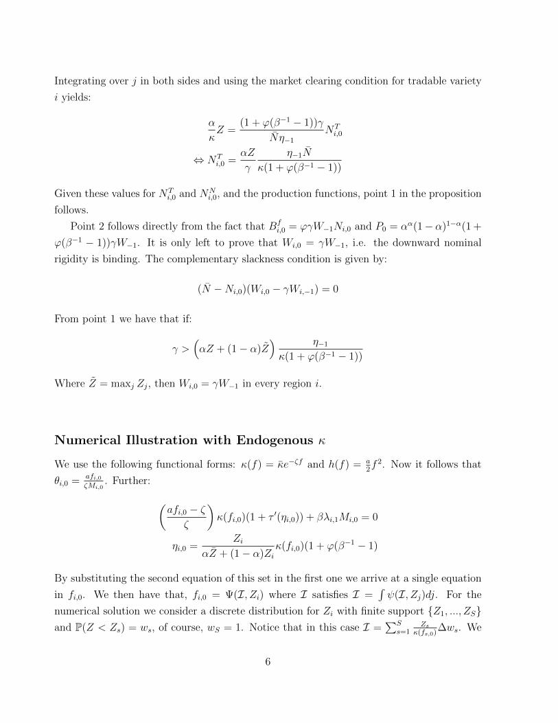
Integrating over j in both sides and using the market clearing condition for tradable variety

i yields:

α

κZ =

(1 + ϕ(β−1 − 1))γ

Nη−1

NTi,0

⇔ NTi,0 =

αZ

γ

η−1N

κ(1 + ϕ(β−1 − 1))

Given these values for NTi,0 and NN

i,0, and the production functions, point 1 in the proposition

follows.

Point 2 follows directly from the fact that Bfi,0 = ϕγW−1Ni,0 and P0 = αα(1− α)1−α(1 +

ϕ(β−1 − 1))γW−1. It is only left to prove that Wi,0 = γW−1, i.e. the downward nominal

rigidity is binding. The complementary slackness condition is given by:

(N −Ni,0)(Wi,0 − γWi,−1) = 0

From point 1 we have that if:

γ >(αZ + (1− α)Z

) η−1

κ(1 + ϕ(β−1 − 1))

Where Z = maxj Zj, then Wi,0 = γW−1 in every region i.

Numerical Illustration with Endogenous κ

We use the following functional forms: κ(f) = κe−ζf and h(f) = a2f 2. Now it follows that

θi,0 =afi,0ζMi,0

. Further:

(afi,0 − ζ

ζ

)κ(fi,0)(1 + τ ′(ηi,0)) + βλi,1Mi,0 = 0

ηi,0 =Zi

αZ + (1− α)Ziκ(fi,0)(1 + ϕ(β−1 − 1)

By substituting the second equation of this set in the first one we arrive at a single equation

in fi,0. We then have that, fi,0 = Ψ(I, Zi) where I satisfies I =∫ψ(I, Zj)dj. For the

numerical solution we consider a discrete distribution for Zi with finite support {Z1, ..., ZS}and P(Z < Zs) = ws, of course, wS = 1. Notice that in this case I =

∑Ss=1

Zsκ(fs,0)

∆ws. We

6

employ the parameter values shown in table A.1.

7

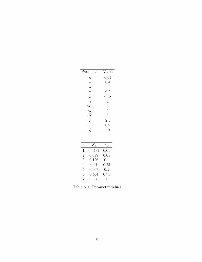
Parameter Value

a 0.01α 0.4κ 1τ 0.2β 0.98γ 1

M−1 1M1 1N 1ν 2.5ϕ 0.9ζ 10

s Zs ws

1 0.0431 0.012 0.089 0.053 0.126 0.14 0.21 0.255 0.307 0.56 0.464 0.757 0.636 1

Table A.1: Parameter values

8

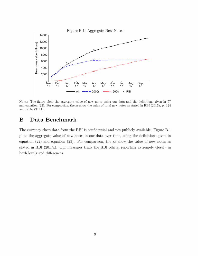
Figure B.1: Aggregate New Notes

0

2000

4000

6000

8000

10000

12000

14000N

ew n

otes

val

ue (b

illio

ns)

Nov16

Dec16

Jan17

Feb17

Mar17

Apr17

May17

Jun17

Jul17

Aug17

Sep17

All 2000s 500s RBI

Notes: The figure plots the aggregate value of new notes using our data and the definitions given in ??and equation (23). For comparsion, the xs show the value of total new notes as stated in RBI (2017a, p. 124and table VIII.1).

B Data Benchmark

The currency chest data from the RBI is confidential and not publicly available. Figure B.1

plots the aggregate value of new notes in our data over time, using the definitions given in

equation (22) and equation (23). For comparison, the xs show the value of new notes as

stated in RBI (2017a). Our measures track the RBI official reporting extremely closely in

both levels and differences.

9

C Further Robustness

C.1 Chests Serving Multiple Districts

Currency chests can serve banks in multiple districts. In this appendix we show that measure-

ment error arising from chests which serve multiple districts would attenuate the empirical

results toward zero.

Recall our baseline cross-sectional specification:

∆yi,t = β0,t + β1,tzi,treatment + ΓtXi + εi,t, (C.1)

where ∆yi,t = lnYi,t− lnYi,baseline denotes the change in the natural logarithm of an outcome

variable relative to the period before demonetization, zi,treatment = lnZi,treatment is the log

of the demonetization shock, and Xi is a vector containing any controls. We construct

zi,treatment by aggregating across currency chests in district i.

Now suppose zi,treatment is a noisy measure of the true demonetization shock, z∗i,treatment,

zi,treatment = z∗i,treatment + ei, (C.2)

where the measurement error ei is mean zero and independent of z∗i,treatment. The measure-

ment error ei could for example stem from not adjusting for chests serving multiple districts.

Thus, the true data generating process replaces zi,treatment in equation (C.1) with z∗i,treatment:

∆yi,t = β∗0,t + β∗1,tz∗i,treatment + Γ∗tXi + ε∗i,t, (C.3)

where E[ε∗i,tei] = E[z∗i,treatmentε∗i,t|Xi] = 0.

To study the consequence of estimating equation (C.1) instead of equation (C.3), let

w⊥i,t denote the residual from projecting a variable wi on a constant and Xi and plim the

10

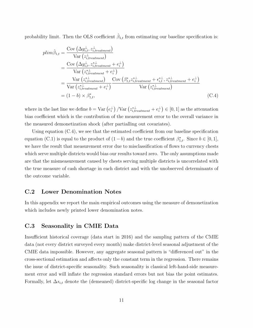
probability limit. Then the OLS coefficient β1,t from estimating our baseline specification is:

plimβ1,t =Cov

(∆y⊥i,t, z

⊥i,treatment

)Var

(z⊥i,treatment

)=

Cov(∆y⊥i,t, z

∗⊥i,treatment + e⊥i

)Var

(z∗⊥i,treatment + e⊥i

)=

Var(z∗⊥i,treatment

)Var

(z∗⊥i,treatment + e⊥i

)Cov(β∗1,tz

∗⊥i,treatment + ε∗⊥i,t , z

∗⊥i,treatment + e⊥i

)Var

(z∗⊥i,treatment

)= (1− b)× β∗1,t, (C.4)

where in the last line we define b = Var(e⊥i)/Var

(z∗⊥i,treatment + e⊥i

)∈ [0, 1] as the attenuation

bias coefficient which is the contribution of the measurement error to the overall variance in

the measured demonetization shock (after partialling out covariates).

Using equation (C.4), we see that the estimated coefficient from our baseline specification

equation (C.1) is equal to the product of (1− b) and the true coefficient β∗1,t. Since b ∈ [0, 1],

we have the result that measurement error due to misclassification of flows to currency chests

which serve multiple districts would bias our results toward zero. The only assumptions made

are that the mismeasurement caused by chests serving multiple districts is uncorrelated with

the true measure of cash shortage in each district and with the unobserved determinants of

the outcome variable.

C.2 Lower Denomination Notes

In this appendix we report the main empirical outcomes using the measure of demonetization

which includes newly printed lower denomination notes.

C.3 Seasonality in CMIE Data

Insufficient historical coverage (data start in 2016) and the sampling pattern of the CMIE

data (not every district surveyed every month) make district-level seasonal adjustment of the

CMIE data impossible. However, any aggregate seasonal pattern is “differenced out” in the

cross-sectional estimation and affects only the constant term in the regression. There remains

the issue of district-specific seasonality. Such seasonality is classical left-hand-side measure-

ment error and will inflate the regression standard errors but not bias the point estimates.

Formally, let ∆si,t denote the (demeaned) district-specific log change in the seasonal factor

11

Figure C.1: ATM Withdrawals Including Lower Denomination Notes in Zi,t

-25.0

-20.0

-15.0

-10.0

-5.0

0.0

Log

chan

ge, O

ct-1

6 to

Dec

-16

-5.0 -4.0 -3.0 -2.0 -1.0 0.0 1.0Log currency replacement rate

-1.0

0.0

1.0

2.0

3.0

4.0

Reg

ress

ion

coef

ficie

nt

Dec15

Mar16

Jun16

Sep16

Dec16

Mar17

Jun17

Sep17

Notes: The left panel presents a scatter plot of the log change in ATM withdrawals between October 2016and December 2016 and the log currency shock. The light blue circles show the raw data and are sizedproportional to 2015 district GDP. The dark red circles average observations into 50 quantile bins of thecurrency shock. The dashed line gives the best fit line. The right panel reports the coefficient and 95%confidence interval from estimating equation (27) for the period indicated on the horizontal axis.

and ∆y∗i,t (demeaned) seasonally-adjusted employment growth, so that ∆y∗i,t = ∆yi,t + ∆si,t

with E[∆si,tzi,treatment] = 0. Comparing the two regression models:

∆y∗i,t = β∗0,t + β∗1,tzi,treatment + Γ∗tXi + ε∗i,t, (C.5)

∆yi,t = β0,t + β1,tzi,treatment + ΓtXi + εi,t, (C.6)

it is apparent that the second equation is equivalent to the first with εi,t = ε∗i,t − ∆si,t.

Therefore, plimβ1,t = plimβ∗1,t, and Var(β1,t

)> Var

(β∗1,t

)because the residual variance is

larger.

12

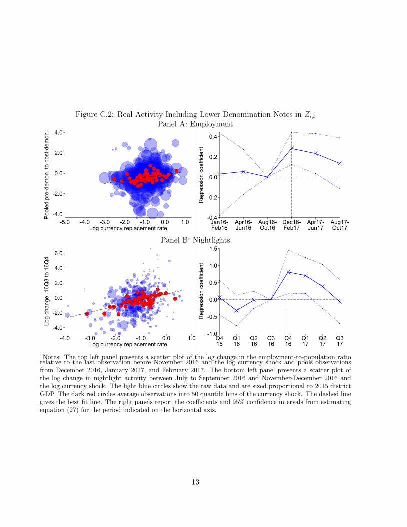
Figure C.2: Real Activity Including Lower Denomination Notes in Zi,tPanel A: Employment

-4.0

-2.0

0.0

2.0

4.0

Pool

ed p

re-d

emon

. to

post

-dem

on.

-5.0 -4.0 -3.0 -2.0 -1.0 0.0 1.0Log currency replacement rate

-0.4

-0.2

0.0

0.2

0.4

Reg

ress

ion

coef

ficie

nt

Jan16-Feb16

Apr16-Jun16

Aug16-Oct16

Dec16-Feb17

Apr17-Jun17

Aug17-Oct17

Panel B: Nightlights

-4.0

-2.0

0.0

2.0

4.0

6.0

Log

chan

ge, 1

6Q3

to 1

6Q4

-4.0 -3.0 -2.0 -1.0 0.0 1.0Log currency replacement rate

-1.0

-0.5

0.0

0.5

1.0

1.5

Reg

ress

ion

coef

ficie

nt

Q415

Q116

Q216

Q316

Q416

Q117

Q217

Q317

Notes: The top left panel presents a scatter plot of the log change in the employment-to-population ratiorelative to the last observation before November 2016 and the log currency shock and pools observationsfrom December 2016, January 2017, and February 2017. The bottom left panel presents a scatter plot ofthe log change in nightlight activity between July to September 2016 and November-December 2016 andthe log currency shock. The light blue circles show the raw data and are sized proportional to 2015 districtGDP. The dark red circles average observations into 50 quantile bins of the currency shock. The dashed linegives the best fit line. The right panels report the coefficients and 95% confidence intervals from estimatingequation (27) for the period indicated on the horizontal axis.

13

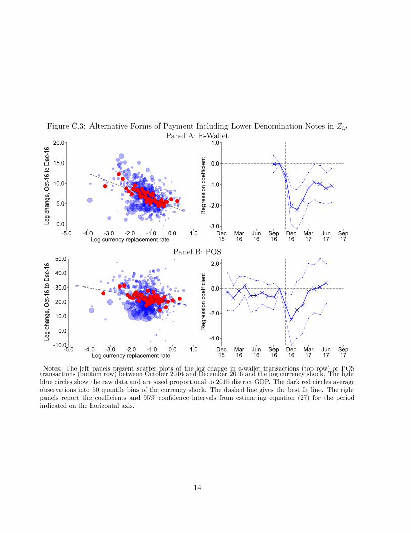
Figure C.3: Alternative Forms of Payment Including Lower Denomination Notes in Zi,tPanel A: E-Wallet

0.0

5.0

10.0

15.0

20.0

Log

chan

ge, O

ct-1

6 to

Dec

-16

-5.0 -4.0 -3.0 -2.0 -1.0 0.0 1.0Log currency replacement rate

-3.0

-2.0

-1.0

0.0

1.0

Reg

ress

ion

coef

ficie

nt

Dec15

Mar16

Jun16

Sep16

Dec16

Mar17

Jun17

Sep17

Panel B: POS

-10.0

0.0

10.0

20.0

30.0

40.0

50.0

Log

chan

ge, O

ct-1

6 to

Dec

-16

-5.0 -4.0 -3.0 -2.0 -1.0 0.0 1.0Log currency replacement rate

-4.0

-2.0

0.0

2.0

Reg

ress

ion

coef

ficie

nt

Dec15

Mar16

Jun16

Sep16

Dec16

Mar17

Jun17

Sep17

Notes: The left panels present scatter plots of the log change in e-wallet transactions (top row) or POStransactions (bottom row) between October 2016 and December 2016 and the log currency shock. The lightblue circles show the raw data and are sized proportional to 2015 district GDP. The dark red circles averageobservations into 50 quantile bins of the currency shock. The dashed line gives the best fit line. The rightpanels report the coefficients and 95% confidence intervals from estimating equation (27) for the periodindicated on the horizontal axis.

14

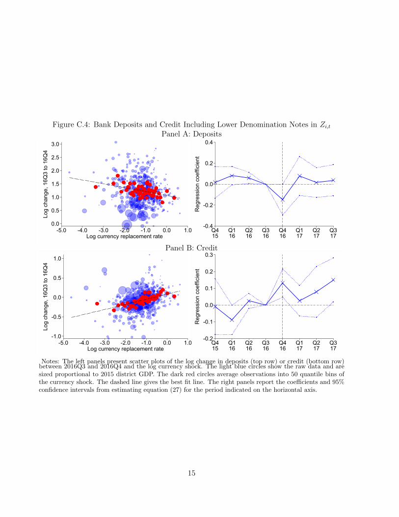
Figure C.4: Bank Deposits and Credit Including Lower Denomination Notes in Zi,tPanel A: Deposits

0.0

0.5

1.0

1.5

2.0

2.5

3.0

Log

chan

ge, 1

6Q3

to 1

6Q4

-5.0 -4.0 -3.0 -2.0 -1.0 0.0 1.0Log currency replacement rate

-0.4

-0.2

0.0

0.2

0.4

Reg

ress

ion

coef

ficie

nt

Q415

Q116

Q216

Q316

Q416

Q117

Q217

Q317

Panel B: Credit

-1.0

-0.5

0.0

0.5

1.0

Log

chan

ge, 1

6Q3

to 1

6Q4

-5.0 -4.0 -3.0 -2.0 -1.0 0.0 1.0Log currency replacement rate

-0.2

-0.1

0.0

0.1

0.2

0.3

Reg

ress

ion

coef

ficie

nt

Q415

Q116

Q216

Q316

Q416

Q117

Q217

Q317

Notes: The left panels present scatter plots of the log change in deposits (top row) or credit (bottom row)between 2016Q3 and 2016Q4 and the log currency shock. The light blue circles show the raw data and aresized proportional to 2015 district GDP. The dark red circles average observations into 50 quantile bins ofthe currency shock. The dashed line gives the best fit line. The right panels report the coefficients and 95%confidence intervals from estimating equation (27) for the period indicated on the horizontal axis.

15