cellular mobile communication - biher · introduction to wireless mobile communication 2....
TRANSCRIPT
CELLULAR MOBILE COMMUNICATION
1

UNIT I
INTRODUCTION TO WIRELESS MOBILE COMMUNICATION
2

Introduction:
In 1897, Guglielmo Marconi first demonstrated radio’s ability to providecontinuous contact with ships sailing the English channel.
During the past 10 years, fueled by Digital and RF circuit fabrication improvements New VLSI technologies Other miniaturization technologies
(e.g., passive components) The mobile communications industry has grown by orders of magnitude.
The trends will continue at an even greater pace during the next decade.
3

Evolution of Mobile Radio Communications
4

In 1934, AM mobile communication systems for municipal police radio systems. Vehicle ignition noise was a major problem.
In 1946, FM mobile communications for the first public mobile telephone service Each system used a single, high-powered transmitter and large tower to cover
distances of over 50 km. Used 120 kHz of RF bandwidth in a half-duplex mode. (push-to-talk release-to-
listen systems.) Large RF bandwidth was largely due to the technology difficulty (in mass-
producing tight RF filter and low-noise, front-end receiver amplifiers.) In 1950, the channel bandwidth was cut in half to 60kHZ due to improved
technology. By the mid 1960s, the channel bandwidth again was cut to 30 kHZ. Thus, from WWII to the mid 1960s, the spectrum efficiency was improved only a
factor of 4 due to the technology advancements.
5

Also in 1950s and 1960s, automatic channel truncking was introducedin IMTS(Improved Mobile Telephone Service.) offering full duplex, auto-dial, auto-trunking became saturated quickly By 1976, has only twelve channels and could only serve 543
customers in New York City of 10 millions populations. Cellular radiotelephone
Developed in 1960s by Bell Lab and others
The basic idea is to reuse the channel frequency at a sufficient distance toincrease the spectrum efficiency.
But the technology was not available to implement until the late 1970s.(mainly the microprocessor and DSP technologies.)
6

In 1983, AMPS (Advanced Mobile Phone System, IS-41) deployed byAmeritech in Chicago.
40 MHz spectrum in 800 MHz band
666 channels (+ 166 channels), per Fig 1.2.
Each duplex channel occupies > 60 kHz (30+30) FDMA to maximizecapacity.
Two cellular providers in each market.
7

8

In late 1991, U.S. Digital Cellular (USDC, IS-54) was introduced.
to replace AMPS analog channels
3 times of capacity due to the use of digital modulation ( DQPSK),
speech coding, and TDMA technologies.
could further increase up to 6 times of capacity given the advancements of
DSP and speech coding technologies.
In mid 1990s, Code Division Multiple Access (CDMA, IS-95) was introduced
by Qualcomm.
based on spread spectrum technology.
supports 6-20 times of users in 1.25 MHz shared by all the channels.
each associated with a unique code sequence.
operate at much smaller SNR.(FdB)
9
4

10

11

Examples of Mobile Radio Systems
12

In FDD,
A device, called a duplexer, is used inside the subscriber unit to enable the
same antenna to be used for simultaneous transmission and reception.
To facilitate FDD, it is necessary to separate the XMIT and RCVD
frequencies by about 5% of the nominal RF frequency, so that the
duplexer can provide sufficient isolation while being inexpensively
manufactured.
In TDD,
Only possible with digital transmission format and digital modulation.
Very sensitive to timing. Consequently, only used for indoor or small area
wireless applications.
13

Paging Systems
14
PAGING CONTROL CENTRE
Paging Terminal
PSTN
Land Line Link
Land Line LinkPaging Terminal
Paging Terminal
City 1
City 2
City N

15
Paging receivers are simple and inexpensive, but the transmission system
required is quite sophisticated. (simulcasting)
designed to provide ultra-reliable coverage, even inside buildings
Buildings can attenuate radio signals by 20 or 30 dB, making the choice of
base station locations difficult for the paging companies.
Small RF bandwidths are used to maximize the signal-to-noise ratio at
each paging receiver, so low data rates (6400 bps or less) are used.

Wireless Local Loop
In the telephone networks, the circuit between the subscriber's equipment (e.g. telephone set) and the local exchange is called the subscriber loop or local loop.
Copper wire has been used as the medium for local loop to provide voice and voice-band data services.
Since 1980s, the demand for communications services has increased explosively. There has been a great need for the basic telephone service, i.e. the plain old telephone service (POTS) in developing countries.
Wireless local loop provides two-ways a telephone system………….. Wireless local loop includes cordless access system, proprietary fixed radio
access system and fixed cellular system. It is also known as fixed radio wireless. This can be in an office or home.
Broadband Wireless Access (BWA), Radio In The Loop (RITL), Fixed-Radio Access (FRA) and Fixed Wireless Access (FWA).
16

Cordless Telephone System
To Connect a Fixed Base Station to a Portable Cordless Handset Early Systems (1980s) have very limited range of few tens of meters [within a
House Premises] Modern Systems [PACS, DECT, PHS, PCS] can provide a limited range &
mobility within Urban Centers
PSTN Fixed Base Station
Cordless Handset
17

Limitations of Simple Mobile Radio Systems The Cellular Approach
Divides the Entire Service Area into Several Small Cells Reuse the Frequency
Basic Components of a Cellular Telephone System Cellular Mobile Phone: A light-weight hand-held set which is an outcome of
the marriage of Graham Bell’s Plain Old Telephone Technology [1876] and Marconi’s Radio Technology [1894] [although a very late delivery but very cute]
Base Station: A Low Power Transmitter, other Radio Equipment [Transceivers] plus a small Tower
Mobile Switching Center [MSC] /Mobile Telephone Switching Office[MTSO] An Interface between Base Stations and the PSTN Controls all the Base Stations in the Region and Processes User ID and
other Call Parameters A typical MSC can handle up to 100,000 Mobiles, and 5000 Simultaneous
Calls Handles Handoff Requests, Call Initiation Requests, and all Billing &
System Maintenance Functions
18

19

The Cellular Concept
RF spectrum is a valuable and scarce commodity RF signals attenuate over distance Cellular network divides coverage area into cells, each served by its own base
station transceiver and antenna Low (er) power transmitters used by BSs; transmission range determines cell
boundary RF spectrum divided into distinct groups of channels Adjacent cells are (usually) assigned different channel groups to avoid
interference Cells separated by a sufficiently large distance to avoid mutual interference can
be assigned the same channel group frequency reuse among co-channel cells
20

Cellular Systems: Reuse channels to maximize capacity
• Geographic region divided into cells• Frequencies/timeslots/codes reused at spatially-separated
locations.• Co-channel interference between same color cells.• Base stations/MTSOs coordinate handoff and control functions• Shrinking cell size increases capacity, as well as networking burden
BASESTATION
MTSO
21

Trends in Cellular radio and Personal Communications
PCS/PCN: PCS calls for more personalized services whereas PCN refers to Wireless Networking Concept-any person, anywhere, anytime can make a call using PC. PCS and PCN terms are sometime used interchangeably
IEEE 802.11: A standard for computer communications using wireless links[inside building].
ETSI’s 20 Mbps HIPER LAN: Standard for indoor Wireless Networks IMT-2000 [International Mobile Telephone-2000 Standard]: A 3G universal,
multi-function, globally compatible Digital Mobile Radio Standard is in making
Satellite-based Cellular Phone Systems A very good Chance for Developing Nations to Improve their Communication
Networks
22

UNIT II
CELLULAR CONCEPT AND SYSTEM DESIGN FUNDAMENTALS
23
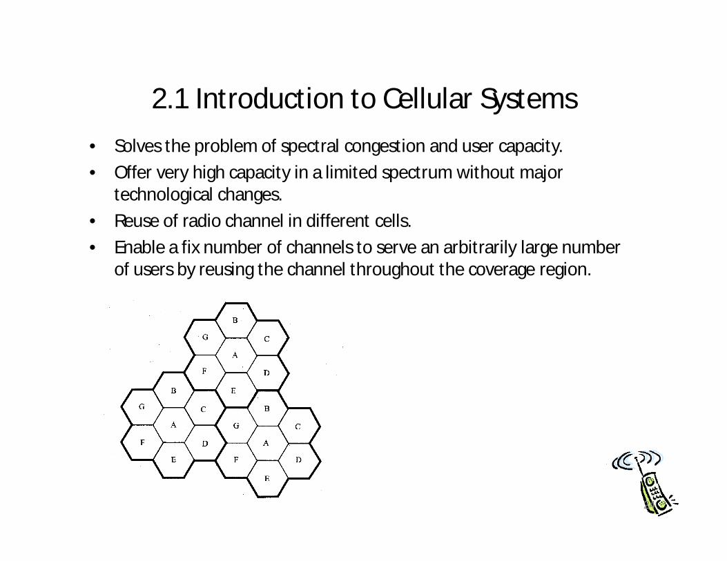
2.1 Introduction to Cellular Systems• Solves the problem of spectral congestion and user capacity.• Offer very high capacity in a limited spectrum without major
technological changes.• Reuse of radio channel in different cells.• Enable a fix number of channels to serve an arbitrarily large number
of users by reusing the channel throughout the coverage region.
24

Frequency Reuse• Each cellular base station is allocated a group of radio channels within
a small geographic area called a cell.• Neighboring cells are assigned different channel groups.• By limiting the coverage area to within the boundary of the cell, the
channel groups may be reused to cover different cells.• Keep interference levels within tolerable limits.• Frequency reuse or frequency planning
•seven groups of channel from A to G
•footprint of a cell - actual radio coverage
•omni-directional antenna v.s. directional antenna
25

• Hexagonal geometry has – exactly six equidistance neighbors– the lines joining the centers of any cell and each of its neighbors are
separated by multiples of 60 degrees.• Only certain cluster sizes and cell layout are possible.• The number of cells per cluster, N, can only have values which satisfy
• Co-channel neighbors of a particular cell, ex, i=3 and j=2.
22 jijiN
26

Channel Assignment Strategies
• Frequency reuse scheme– increases capacity– minimize interference
• Channel assignment strategy– fixed channel assignment– dynamic channel assignment
• Fixed channel assignment– each cell is allocated a predetermined set of voice channel– any new call attempt can only be served by the unused channels– the call will be blocked if all channels in that cell are occupied
• Dynamic channel assignment– channels are not allocated to cells permanently.– allocate channels based on request.– reduce the likelihood of blocking, increase capacity.
27

2.4 Handoff Strategies
• When a mobile moves into a different cell while a conversation is in progress, the MSC automatically transfers the call to a new channel belonging to the new base station.
• Handoff operation– identifying a new base station– re-allocating the voice and control channels with the new base station.
• Handoff Threshold– Minimum usable signal for acceptable voice quality (-90dBm to -100dBm)– Handoff margin cannot be too large or too
small.– If is too large, unnecessary handoffs burden the MSC– If is too small, there may be insufficient time to complete handoff
before a call is lost.
usable minimum,, rhandoffr PP
28

29

• Handoff must ensure that the drop in the measured signal is not due to momentary fading and that the mobile is actually moving away from the serving base station.
• Running average measurement of signal strength should be optimized so that unnecessary handoffs are avoided.
– Depends on the speed at which the vehicle is moving.– Steep short term average -> the hand off should be made quickly– The speed can be estimated from the statistics of the received short-term
fading signal at the base station• Dwell time: the time over which a call may be maintained within a cell
without handoff.• Dwell time depends on
– propagation– interference– distance– speed
30

• Handoff measurement– In first generation analog cellular systems, signal strength measurements
are made by the base station and supervised by the MSC.– In second generation systems (TDMA), handoff decisions are mobile
assisted, called mobile assisted handoff (MAHO) • Intersystem handoff: If a mobile moves from one cellular system to a
different cellular system controlled by a different MSC.• Handoff requests is much important than handling a new call.
31

Practical Handoff Consideration
• Different type of users– High speed users need frequent handoff during a call.– Low speed users may never need a handoff during a call.
• Microcells to provide capacity, the MSC can become burdened if high speed users are constantly being passed between very small cells.
• Minimize handoff intervention– handle the simultaneous traffic of high speed and low speed users.
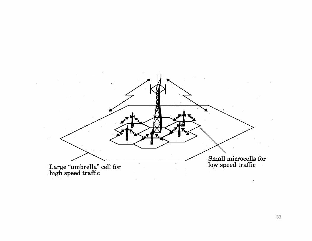
• Large and small cells can be located at a single location (umbrella cell) – different antenna height– different power level
• Cell dragging problem: pedestrian users provide a very strong signal to the base station
– The user may travel deep within a neighboring cell
32
33

• Handoff for first generation analog cellular systems– 10 secs handoff time– is in the order of 6 dB to 12 dB
• Handoff for second generation cellular systems, e.g., GSM– 1 to 2 seconds handoff time– mobile assists handoff– is in the order of 0 dB to 6 dB– Handoff decisions based on signal strength, co-channel interference, and
adjacent channel interference.• IS-95 CDMA spread spectrum cellular system
– Mobiles share the channel in every cell.– No physical change of channel during handoff– MSC decides the base station with the best receiving signal as the service
station
•
34

Types of Handoffs: Hard handoff: “break before make” connection Intra and inter-cell handoffs
Hard Handoff between the MS and BSs
35

Cont.
Soft handoff: “make-before-break” connection.Mobile directed handoff. Multiways and softer handoffs
Soft Handoff between MS and BSTs
36

Handoff Prioritization:
Two basic methods of handoff prioritization are : Guard Channels Queuing of Handoff
37

2.5 Interference and System Capacity
• Sources of interference– another mobile in the same cell– a call in progress in the neighboring cell– other base stations operating in the same frequency band– noncellular system leaks energy into the cellular frequency band
• Two major cellular interference– co-channel interference– adjacent channel interference
38

2.5.1 Co-channel Interference and System Capacity
• Frequency reuse - there are several cells that use the same set of frequencies
– co-channel cells– co-channel interference
• To reduce co-channel interference, co-channel cell must be separated by a minimum distance.
• When the size of the cell is approximately the same– co-channel interference is independent of the transmitted power– co-channel interference is a function of
• R: Radius of the cell • D: distance to the center of the nearest co-channel cell
• Increasing the ratio Q=D/R, the interference is reduced.• Q is called the co-channel reuse ratio
39

• For a hexagonal geometry
• A small value of Q provides large capacity• A large value of Q improves the transmission quality - smaller level of
co-channel interference• A tradeoff must be made between these two objectives
NRDQ 3
40

• Let be the number of co-channel interfering cells. The signal-to-interference ratio (SIR) for a mobile receiver can be expressed as
S: the desired signal power: interference power caused by the ith interfering co-channel cell
base station• The average received power at a distance d from the transmitting
antenna is approximated by
or
n is the path loss exponent which ranges between 2 and 4.
0i
0
1
i
iiI
SIS
iI
n
r ddPP
00
00 log10)dBm()dBm(
ddnPPr
close-in reference point
TX
0d
0P :measued power
41

• When the transmission power of each base station is equal, SIR for a mobile can be approximated as
• Consider only the first layer of interfering cells
0
1
i
i
ni
n
D
RIS
00
3)/(iN
iRD
IS
nn
• Example: AMPS requires that SIR be greater than 18dB
– N should be at least 6.49 for n=4.– Minimum cluster size is 7
60 i
42

• For hexagonal geometry with 7-cell cluster, with the mobile unit being at the cell boundary, the signal-to-interference ratio for the worst case can be approximated as
44444
4
)()2/()2/()(2
DRDRDRDRDR
IS
43

2.5.2 Adjacent Channel Interference
• Adjacent channel interference: interference from adjacent in frequency to the desired signal.
– Imperfect receiver filters allow nearby frequencies to leak into the passband
– Performance degrade seriously due to near-far effect.
desired signal
receiving filter response
desired signalinterference
interference
signal on adjacent channelsignal on adjacent channel
FILTER
44

• Adjacent channel interference can be minimized through careful filtering and channel assignment.
• Keep the frequency separation between each channel in a given cell as large as possible
• A channel separation greater than six is needed to bring the adjacent channel interference to an acceptable level.
• Ensure each mobile transmits the smallest power necessary to maintain a good quality link on the reverse channel
– long battery life– increase SIR– solve the near-far problem
45

Trunking and Grade of Service
A means for providing access to users on demand from available pool of channels.With trunking, a small number of channels can accommodate large number of
random users.Telephone companies use trunking theory to determine number of circuits required.Trunking theory is about how a population can be handled by a limited number of
servers.
46

Terminology:
Traffic intensity is measured in Erlangs:One Erlang: traffic in a channel completely occupied. 0.5 Erlang: channel occupied
30 minutes in an hour.Grade of Service (GOS): probability that a call is blocked (or delayed).Set-Up Time: time to allocate a channel.Blocked Call: Call that cannot be completed at time of request due to congestion.
Also referred to as Lost Call.Holding Time: (H) average duration of typical call.Load: Traffic intensity across the whole system.Request Rate: (λ) average number of call requests per unit time.
47

Traffic Measurement (Erlangs)
48

49

50

51

52

53

54
55

Erlang C Model –Blocked calls cleared
A different type of trunked system queues blocked calls –Blocked Calls Delayed. This is known as an Erlang C model.
Procedure:
Determine Pr[delay> 0] = probability of a delay from the chart. Pr[delay > t | delay > 0 ] = probability that the delay is longer than t, given
that there is a delay Pr[delay > t | delay > 0 ] =exp[-(C-A)t /H ] Unconditional Probability of delay > t : Pr[delay > t ] = Pr[delay > 0] Pr[delay > t | delay > 0 ] Average delay time D = Pr[delay > 0] H/ (C-A)
56

Erlang C Formula
The likelihood of a call not having immediate access to a channel is determinedby Erlang C formula:
57

58

59

60

2.7 Improving Capacity in Cellular Systems
• Methods for improving capacity in cellular systems– Cell Splitting: subdividing a congested cell into smaller cells.– Sectoring: directional antennas to control the interference and frequency
reuse.– Coverage zone : Distributing the coverage of a cell and extends the cell
boundary to hard-to-reach place.
61

Cell Splitting
Cell Splitting is the process of subdividing the congested cell into smallercells (microcells),Each with its own base station and a correspondingreduction in antenna height and transmitter power.
Cell Splitting increases the capacity since it increases the number of timesthe channels are reused.
62

2.7.1 Cell Splitting• Split congested cell into smaller cells.
– Preserve frequency reuse plan.– Reduce transmission power.
microcell
Reduce R to R/2
63

Illustration of cell splitting within a 3 km by 3 km square
64

• Transmission power reduction from to • Examining the receiving power at the new and old cell boundary
• If we take n = 4 and set the received power equal to each other
• The transmit power must be reduced by 12 dB in order to fill in the original coverage area.
• Problem: if only part of the cells are splited– Different cell sizes will exist simultaneously
• Handoff issues - high speed and low speed traffic can be simultaneously accommodated
1tP 2tP
ntr RPP 1]boundary cell oldat [
ntr RPP )2/(]boundary cellnew at [ 2
161
2t
tPP
65

2.7.2 Sectoring• Decrease the co-channel interference and keep the cell radius R
unchanged– Replacing single omni-directional antenna by several directional antennas– Radiating within a specified sector
66

• Interference Reduction
position of the mobile
interference cells
67

2.7.3 Microcell Zone Concept• Antennas are placed at the outer edges of the cell• Any channel may be assigned to any zone by the base station• Mobile is served by the zone with the strongest signal.
• Handoff within a cell– No channel re-
assignment– Switch the channel to a
different zone site• Reduce interference
– Low power transmitters are employed
68
Multiple Access Techniques for WirelessCommunication:
Many users can access the at same time, share a finite amount of radio spectrum with high performance duplexing generally required frequency domain time domain. They accessing techniques are,
FDMA TDMA SDMA PDMA
69

Frequency division multiple access FDMA
One phone circuit per channel Idle time causes wasting of resources Simultaneously and continuously transmitting Usually implemented in narrowband systems For example: in AMPS is a FDMA bandwidth of 30 kHz implemented
70
Time Division Multiple Access Time slots One user per slot Buffer and burst method Noncontinuous transmission Digital data
Digital modulation
71

Features of TDMA A single carrier frequency for several users Transmission in bursts Low battery consumption Handoff process much simpler FDD : switch instead of duplexer Very high transmission rate High synchronization overhead Guard slots necessary
72

Space Division Multiple Access
Controls radiated energy for each user in space using spot beam antennas base station tracks user when moving cover areas with same frequency: TDMA or CDMA systems cover areas with same frequency: FDMA systems
73

Space Division Multiple Access
primitive applications are “Sectorizedantennas”
In future adaptive antennas simultaneouslysteer energy in the direction of many users atonce
74

UNIT III
MOBILE RADIO PROPAGATION
75
76
. Mobile Radio Propagation• RF channels are random – do not offer easy analysis• difficult to model – typically done statistically for a specific system
Introduction to Radio Wave Propagation: diverse mechanisms of electromagnetic (EM) wave propagation generally attributed to
(i) diffraction(ii) reflection(iii) scattering
• non-line of sight (NLOS – obstructed) paths rely on reflections• obstacles cause diffraction• multi-path: EM waves travel on different paths to a destination –interaction of paths causes fades at specific locations

77
traditional Propagation Models focus on (i) transmit model - average received signal strength at given distance
(ii) receive model - variability in signal strength near a given location
(1) Large Scale Propagation Models: predict mean signal strength for TX-RX pair with arbitrary separation
• useful for estimating coverage area of a transmitter
• characterizes signal strength over large distances (102-103 m)
• predict local average signal strength that decreases with
distance

78
(2) Small Scale or Fading Models: characterize rapid fluctuations of received signal over
• short distances (few ) or • short durations (few seconds)
with mobility over short distances
• instantaneous signal strength fluctuates• received signal = sum of many components from different directions• phases are random sum of contributions varies widely• received signal may fluctuate 30-40 dB by moving a fraction of

Large-scale small-scale propagation
79

Reflection
• Perfect conductors reflect with no attenuation– Like light to the mirror
• Dielectrics reflect a fraction of incident energy– “Grazing angles” reflect max*– Steep angles transmit max*– Like light to the water
• Reflection induces 180 phase shift– Why? See yourself in the mirror
q qr
qt
80

Classical 2-ray ground bounce model
• One line of sight and one ground bound
81
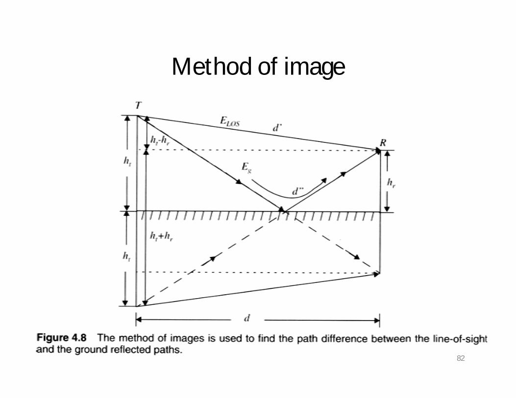
Method of image
82

Vector addition of 2 rays
83

Simplified model
• Far field simplified model• Example 2.2
4
22
dhhGGPP rt
rttr
84

Diffraction• Diffraction occurs when waves hit the edge of an obstacle
– “Secondary” waves propagated into the shadowed region– Water wave example– Diffraction is caused by the propagation of secondary wavelets
into a shadowed region. – Excess path length results in a phase shift– The field strength of a diffracted wave in the shadowed region is
the vector sum of the electric field components of all the secondary wavelets in the space around the obstacle.
– Huygen’s principle: all points on a wavefront can be considered as point sources for the production of secondary wavelets, and that these wavelets combine to produce a new wavefront in the direction of propagation.
85

Diffraction geometry
• Fresnel-Kirchoff distraction parameters,
86

Fresnel Screens• Fresnel zones relate phase shifts to the
positions of obstacles• A rule of thumb used for line-of-sight
microwave links 55% of the first Fresnel zone is kept clear.
87
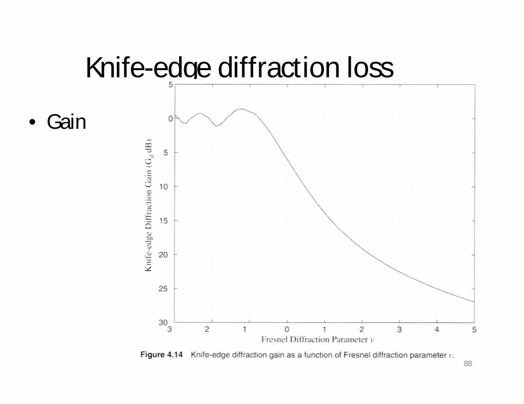
Knife-edge diffraction loss
• Gain
88

Scattering
• Rough surfaces– Lamp posts and trees, scatter all directions– Critical height for bumps is f(,incident angle),– Smooth if its minimum to maximum protuberance h is less
than critical height.– Scattering loss factor modeled with Gaussian distribution,
• Nearby metal objects (street signs, etc.)– Usually modeled statistically
• Large distant objects– Analytical model: Radar Cross Section (RCS)– Bistatic radar equation,
89

Impulse Response Model of a Time Variant Multipath Channel
90

91
3.2 Free Space Propagation Modelused to predict signal strength for LOS path
• satellites• LOS uwave• power decay d –n (d = separation)
Subsections
(1) Friis Equation
(2) Radiated Power
(3) Path Loss
(4) Far Field Region
92
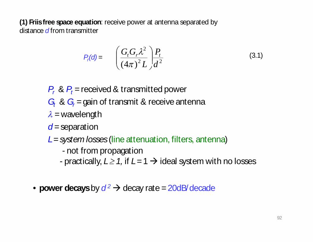
(1) Friis free space equation: receive power at antenna separated by distance d from transmitter
Pr(d) = 22
2
)4( dP
LGG trt
(3.1)
Pr & Pt = received & transmitted powerGt & Gr = gain of transmit & receive antenna = wavelengthd = separationL = system losses (line attenuation, filters, antenna)
- not from propagation - practically, L 1, if L = 1 ideal system with no losses
• power decays by d 2 decay rate = 20dB/decade

93
Antenna Efficiency η = Ae/A
• for parabolic antenna η 45% - 50%• for horn antenna η 50% - 80%
A = antenna’s physical area (cross sectional)
G = eA24
(3.2)
• Ae = effective area of absorption– related to antenna size
Antenna Gain

94
Effective Area of isotropic antennae given by Aiso = 4
2
• f 2 relationship with antenna size results from dependence of Aiso on
Isotropic free space path loss Lp =
2
24d
PP
R
T
TT Pd
Pd 2
2
2
2
441
4
PR =Isotropic Received Power
• d = transmitter-receiver separation
(2) Radiated Power
Isotropic Radiator: ideal antenna (used as a reference antenna)• radiates power with unit gain uniformly in all directions• surface area of a sphere = 4πd 2

95
Directional Radiationpractical antennas have gain or directivity that is a function of
• θ = azimuth: look angle of the antenna in the horizontal plane • = elevation: look angle of the antenna above the horizontal plane
Let Φ = power flux desnity
transmit antenna gain is given by:
GT(θ, ) = Φ in the direction of (θ, )Φ of isotropic antenna
receive antenna gain is given by:
GR(θ, ) = Ae in the direction of (θ, )Ae of isotropic antenna
θ

96
Principal Of Reciprocity:• signal transmission over a radio path is reciprocal
• the locations of TX & RX can be interchanged without changing transmission characteristics
signals suffers exact same effects over a path in either direction in a consistent order implies that GT(θ, ) = GR(θ, )
thus maximum antenna gain in either direction is given by
G = eiso
e AAA
24

97
ERP: effective radiated power - often used in practice • denotes maximum radiated power compared to ½ wave dipole antenna
• dipole antenna gain = 1.64 (2.15dB) > isotropic antenna• thus EIRP will be 2.15dB smaller than ERP for same system
EIRP: effective isotropic radiated power• represents maximum radiated power available from a transmitter• measured in the direction of maximum antenna gain as compared to isotropic radiator
EIRP = PtGiso (3.4)
ERP = PtGdipole

• 1. Outdoor Propagation Models– 1.1 Longley-Rice Model– 1.2 Okumura Model– 1.3. Hata Model– 1.4. PCS Extension to Hata Model– 1.5. Walfisch and Bertoni Model
98

Outdoor Propagation Models
• Propagation over irregular terrain.• The propagation models available for
predicting signal strength vary very widely intheir capacity, approach, and accuracy.
99

Longley-Rice Model
• also referred to as the ITS irregular terrain model
• frequency range from 40 MHz to 100 GHz• Two version:• point-to-point using terrain profile. • area mode estimate the path-specific
parameters
100

Okumura Model• Frequency range from150 MHz to 1920 MHz• BS-MS distance of 1 km to 100 km.• BS antenna heights ranging from 30 m 1000 m.
• Lf is the free space propagation loss, • Amu is the median attenuation relative to free space, • G(tte ) is the base station antenna height gain factor, G(tre ) is
the mobile antenna height gain factor, • GAREA is the gain due to the type of environment.
AREAretemuf GhGhGdfALdBL )()(),()(50
101

Hata Model • Frequency range from150 MHz to 1500 MHz• BS-MS distance of 1 km to 100 km.• BS antenna heights ranging from 30 m 200 m.
• fc is the frequency (in MHz) from 150 MHz to 1500 MHz, • hte is the effective transmitter antenna height (in meters) • hre is the effective receiver (mobile) antenna height (1..10 m)• d is the T-R separation distance (in km),• a(hre ) is the correction factor for effective mobile antenna
height (large city, small to medium size city, suburban, open rural)
dhhahfdBurbanL teretec loglog55.69.44log82.13log16.2655.69)(50
102

PCS Extension to Hata Model• Frequency range from1500 MHz to 2000 MHz• BS-MS distance of 1 km to 20 km.• BS antenna heights ranging from 30 m 200 m.
• fc is the frequency (in MHz) from 1500 MHz to 2000 MHz, • hte is the effective transmitter antenna height (in meters) • hre is the effective receiver (mobile) antenna height (1..10 m)• d is the T-R separation distance (in km),• a(hre ) is the correction factor for effective mobile antenna height
(large city, small to medium size city, suburban, open rural)• CM 0 dB for medium sized city and suburban areas,• 3 dB for metropolitan centers
Mteretec CdhhahfurbanL loglog55.69.44log82.13log9.333.4650
103
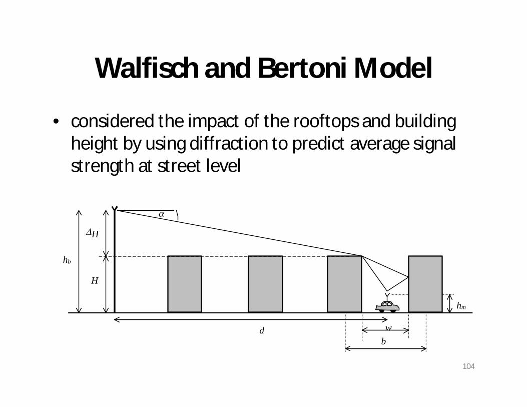
Walfisch and Bertoni Model
• considered the impact of the rooftops and building height by using diffraction to predict average signal strength at street level
H
hb
dbw
hm
H
104

Indoor Propagation Models
• The distances covered are much smaller• The variability of the environment is much greater• Key variables: layout of the building, construction
materials, building type, where the antennamounted, …etc.
• In general, indoor channels may be classified either asLOS or OBS with varying degree of clutter
• The losses between floors of a building are determined by the external dimensions and materials of the building, as well as the type of construction used to create the floors and the external surroundings.
• Floor attenuation factor (FAF)
105

Partition losses between floors
106

Partition losses between floors
107

Log-distance Path Loss Model• The exponent
n depends on the surroundings and building type– X is the
variable in dB having a standard deviation .PL d PL d n d d X( ) ( ) log( / ) 0 010
108

Ericsson Multiple Breakpoint Model
109

Attenuation Factor Model
• FAF represents a floor attenuation factor for a specified number of building floors.
• PAF represents the partition attenuation factor for a specific obstruction encountered by a ray drawn between the transmitter and receiver in 3-D
• is the attenuation constant for the channel with units of dB per meter.
FAFddndPLdPL SF )/log(10)()( 00
PL d PL d n d dMF( ) ( ) log( / ) 0 010
PL d PL d d d d FAF( ) ( ) log( / ) 0 010
PAF
PAF
PAF
110
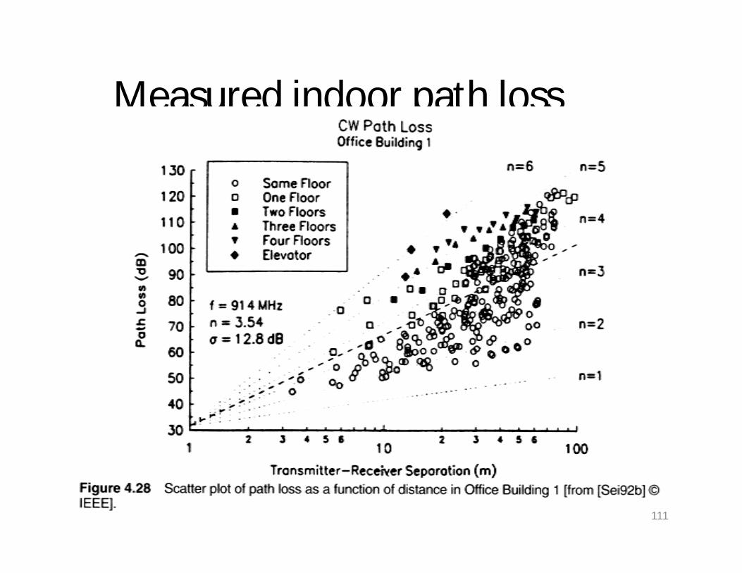
Measured indoor path loss
111

Measured indoor path loss
112

Measured indoor path loss
113

Parameters of Mobile Multipath Channels
• Time Dispersion Parameters– Grossly quantifies the multipath channel– Determined from Power Delay Profile– Parameters include
– Mean Access Delay– RMS Delay Spread– Excess Delay Spread (X dB)
• Coherence Bandwidth• Doppler Spread and Coherence Time
114

Measuring PDPs
• Power Delay Profiles– Are measured by channel sounding techniques– Plots of relative received power as a function of
excess delay – They are found by averaging intantenous power
delay measurements over a local area– Local area: no greater than 6m outdoor– Local area: no greater than 2m indoor
» Samples taken at /4 meters approximately» For 450MHz – 6 GHz frequency range.
115

Timer Dispersion Parameters
kk
kkk
kk
kkk
P
P
a
a
)(
))(( 2
2
22
2
22
kk
kkk
kk
kkk
P
P
a
a
)(
))((
2
2
Determined from a power delay profile.
Mean excess delay( ):
Rms delay spread (st):
116
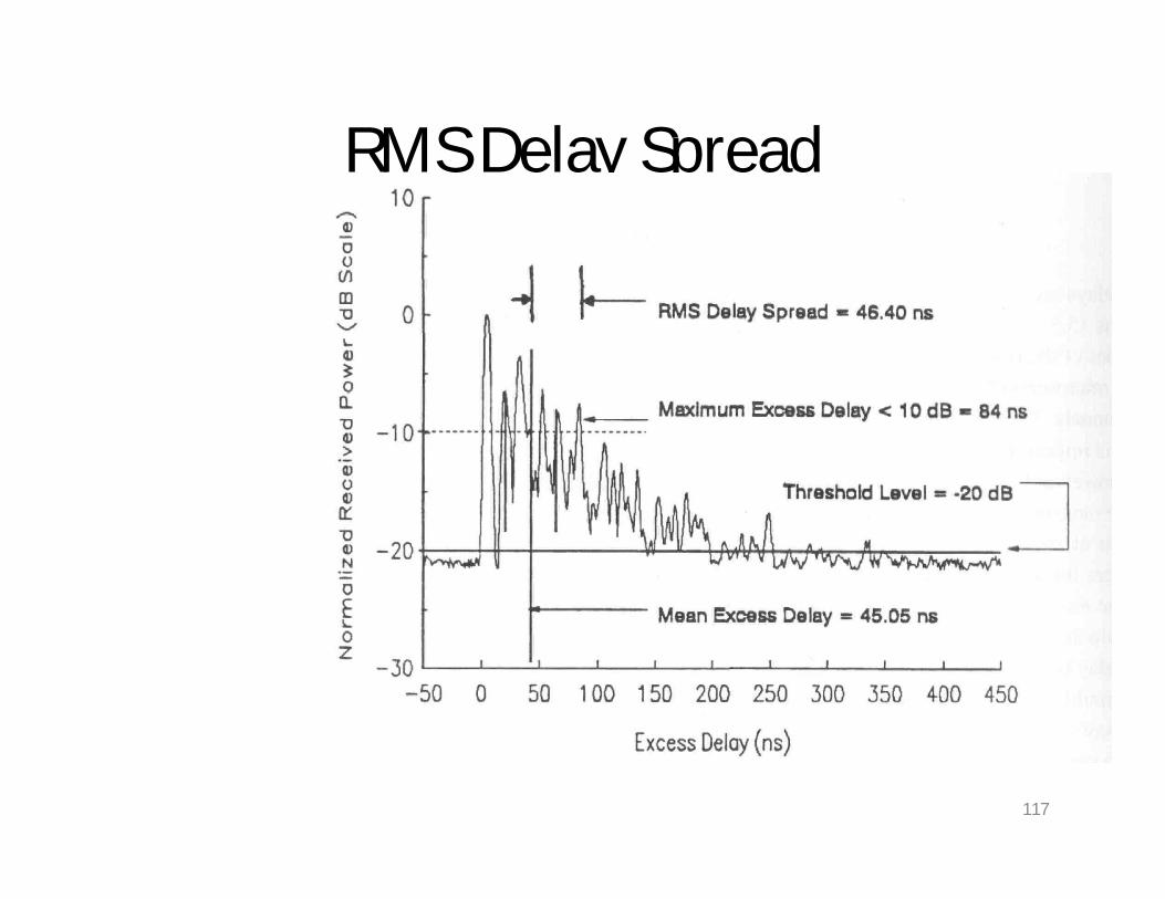
RMS Delay Spread
117

Coherence Bandwidth (BC)– Range of frequencies over which the channel can be
considered flat (i.e. channel passes all spectral components with equal gain and linear phase).
– It is a definition that depends on RMS Delay Spread.
– Two sinusoids with frequency separation greater than Bc are affected quite differently by the channel.
Receiver
f1
f2
Multipath Channel Frequency Separation: |f1-f2|
118

Coherence Bandwidth
501
CB
51
CB
Frequency correlation between two sinusoids: 0 <= Cr1, r2 <= 1.
If we define Coherence Bandwidth (BC) as the range of frequencies over which the frequency correlation is above 0.9, then
If we define Coherence Bandwidth as the range of frequencies over which the frequency correlation is above 0.5, then
is rms delay spread.
This is called 50% coherence bandwidth.
119
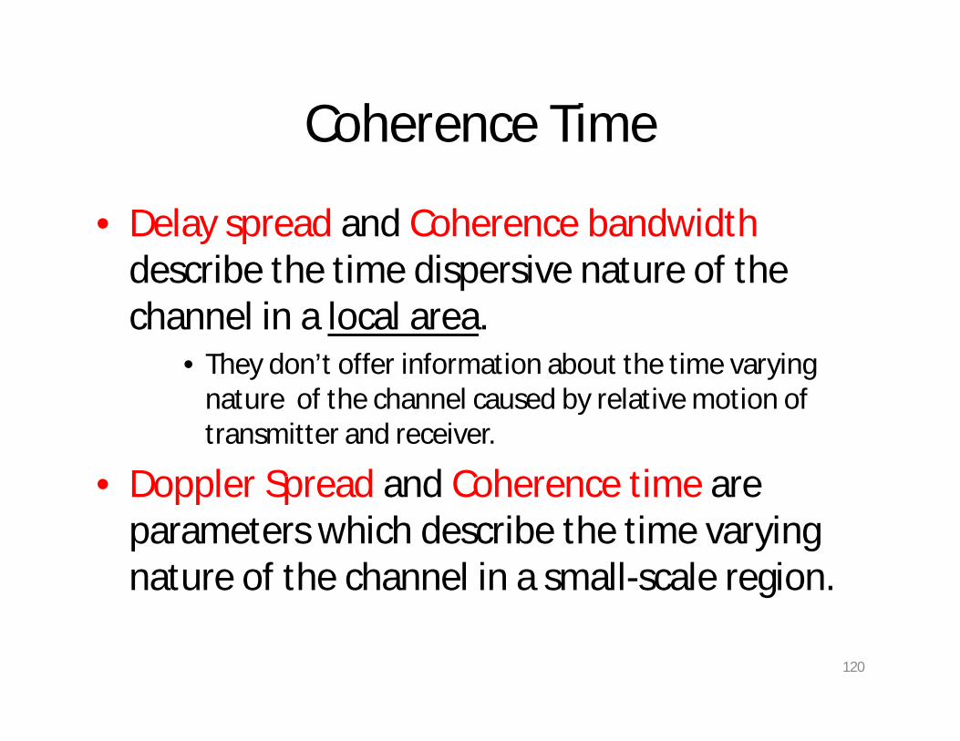
Coherence Time
• Delay spread and Coherence bandwidthdescribe the time dispersive nature of the channel in a local area.
• They don’t offer information about the time varying nature of the channel caused by relative motion of transmitter and receiver.
• Doppler Spread and Coherence time are parameters which describe the time varying nature of the channel in a small-scale region.
120

Doppler Spread
• Measure of spectral broadening caused by motion
• We know how to compute Doppler shift: fd
• Doppler spread, BD, is defined as the maximum Doppler shift: fm = v/
• If the baseband signal bandwidth is much greater than BD then effect of Doppler spread is negligible at the receiver.
121

Coherence Time
mfCT 1
Coherence time is the time duration over which the channel impulse responseis essentially invariant.
If the symbol period of the baseband signal (reciprocal of the baseband signal bandwidth) is greater the coherence time, than the signal will distort, sincechannel will change during the transmission of the signal .
Coherence time (TC) is defined as: TS
TC
t=t2 - t1t1 t2
f1f2
122

Coherence Time
mfC f
Tm
423.0216
9
Coherence time is also defined as:
Coherence time definition implies that two signals arriving with a time separation greater than TC are affected differently by the channel.
123
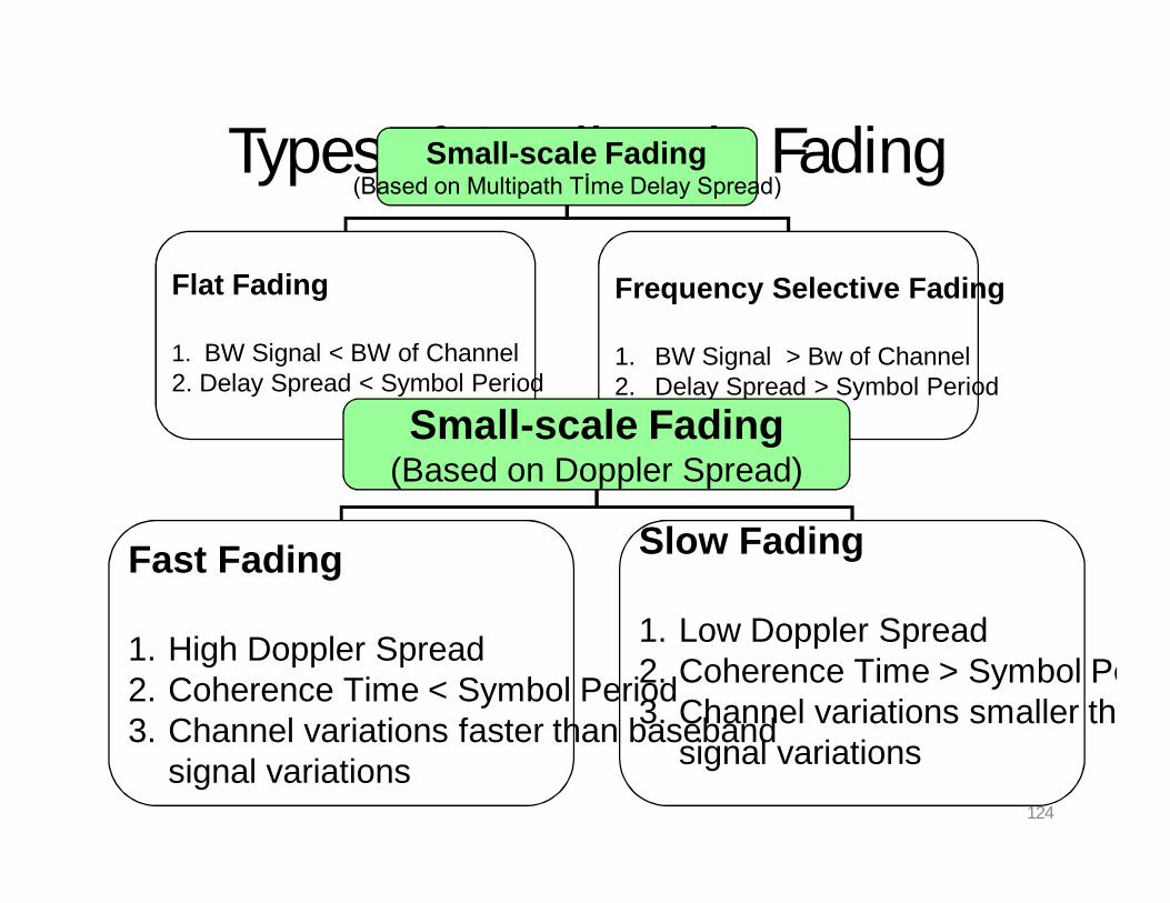
Types of Small-scale FadingSmall-scale Fading(Based on Multipath Tİme Delay Spread)
Flat Fading
1. BW Signal < BW of Channel 2. Delay Spread < Symbol Period
Frequency Selective Fading
1. BW Signal > Bw of Channel2. Delay Spread > Symbol Period
Small-scale Fading(Based on Doppler Spread)
Fast Fading
1. High Doppler Spread2. Coherence Time < Symbol Period3. Channel variations faster than baseband
signal variations
Slow Fading
1. Low Doppler Spread2. Coherence Time > Symbol Period3. Channel variations smaller than baseband
signal variations124

Flat Fading
• Occurs when the amplitude of the receivedsignal changes with time
• For example according to Rayleigh Distribution
• Occurs when symbol period of the transmitted signal is much larger than the Delay Spread of the channel
– Bandwidth of the applied signal is narrow.
• May cause deep fades. – Increase the transmit power to combat this situation.
125

Flat Fadingh(t,ts(t) r(t)
0 TS 0 t 0 TS+t
t << TS
Occurs when:BS << BC
andTS >> t
BC: Coherence bandwidthBS: Signal bandwidthTS: Symbol periodt: Delay Spread
126

Frequency Selective Fading
• Occurs when channel multipath delay spread is greater than the symbol period. – Symbols face time dispersion– Channel induces Intersymbol Interference (ISI)
• Bandwidth of the signal s(t) is wider than the channel impulse response.
127

Frequency Selective Fadingh(t,ts(t) r(t)
0 TS 0 t 0 TS+t
t >> TS
TS
Causes distortion of the received baseband signal
Causes Inter-Symbol Interference (ISI)
Occurs when:BS > BC
andTS < t
As a rule of thumb: TS < t
128

Fast Fading• Due to Doppler Spread
• Rate of change of the channel characteristicsis larger than the
Rate of change of the transmitted signal• The channel changes during a symbol period. • The channel changes because of receiver motion. • Coherence time of the channel is smaller than the symbol period
of the transmitter signal
Occurs when:BS < BD
andTS > TC
BS: Bandwidth of the signalBD: Doppler SpreadTS: Symbol PeriodTC: Coherence Bandwidth
129

Slow Fading
• Due to Doppler Spread• Rate of change of the channel characteristics
is much smaller than theRate of change of the transmitted signal
Occurs when:BS >> BD
andTS << TC
BS: Bandwidth of the signalBD: Doppler SpreadTS: Symbol PeriodTC: Coherence Bandwidth
130

Different Types of Fading
Transmitted Symbol Period
Symbol Period ofTransmitting Signal
TS
TS
TC
t
Flat SlowFading
Flat Fast Fading
Frequency SelectiveSlow Fading
Frequency Selective Fast Fading
With Respect To SYMBOL PERIOD
131

Antennas: simple dipoles Real antennas are not isotropic radiators but, e.g., dipoles with lengths /4 on car
roofs or /2 as Hertzian dipole shape of antenna proportional to wavelength
Example: Radiation pattern of a simple Hertzian dipole
Gain: maximum power in the direction of the main lobe compared to the power ofan isotropic radiator (with the same average power)
side view (xy-plane)
x
y
side view (yz-plane)
z
y
top view (xz-plane)
x
z
simpledipole
/4 /2
132

Antennas: Directed and Sectorized Often used for microwave connections or base stations for mobile phones (e.g.,
radio coverage of a valley)
side view (xy-plane)
x
y
side view (yz-plane)
z
y
top view (xz-plane)
x
z
top view, 3 sector
x
z
top view, 6 sector
x
z
directedantenna
sectorizedantenna
133

UNIT IV
MODULATION AND SIGNAL PROCESSING
134

Modulation Techniques
Modulation can be done by varying the
Amplitude
Phase, or
Frequency of a high frequency carrier in accordance with the amplitude of the message signal.
Demodulation is the inverse operation: extracting the baseband message from the carrier so that it may be processed at the receiver.
135

Analog/Digital Modulation
Analog Modulation
The input is continues signal
Used in first generation mobile radio systems such as AMPS in USA.
Digital Modulation
The input is time sequence of symbols or pulses.
Are used in current and future mobile radio systems
136

Goal of Modulation Techniques
Modulation is difficult task given the hostile mobile radio channels
Small-scale fading and multipath conditions.
The goal of a modulation scheme is:
Transport the message signal through the radio channel with best possible quality
Occupy least amount of radio (RF) spectrum.
137

Amplitude Modulation
138

Double Sideband Spectrum
139
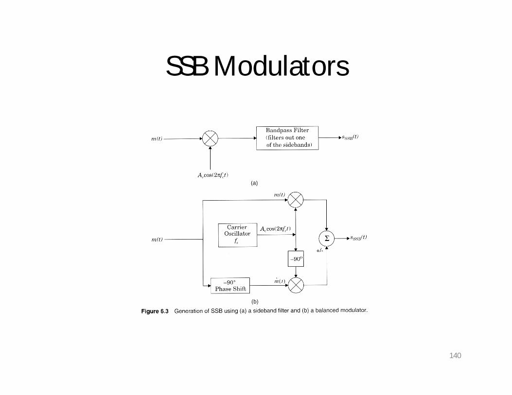
SSB Modulators
140

Wideband FM generation
141

Slope Detector for FM
142

Digital Modulation
The input is discrete signals
Time sequence of pulses or symbols
Offers many advantages
Robustness to channel impairments
Easier multiplexing of variuous sources of information: voice, data, video.
Can accommodate digital error-control codes
Enables encryption of the transferred signals
More secure link
143

Factors that Influence Choice of Digital Modulation Techniques
A desired modulation scheme
Provides low bit-error rates at low SNRs
o Power efficiency
Performs well in multipath and fading conditions
Occupies minimum RF channel bandwidth
o Bandwidth efficiency
Is easy and cost-effective to implement
Depending on the demands of a particular system or application, tradeoffs are made when selecting a digital modulation scheme.
144
Power Efficiency of Modulation
Power efficiency is the ability of the modulation technique to preserve fidelity of the message at low power levels.
Usually in order to obtain good fidelity, the signal power needs to be increased.
Tradeoff between fidelity and signal power
Power efficiency describes how efficient this tradeoff is made
PER
NEb
p :EfficiencyPower certainfor input receiver at the required0
Eb: signal energy per bit
N0: noise power spectral density
PER: probability of error 145

Bandwidth Efficiency of Modulation
Ability of a modulation scheme to accommodate data within a limited bandwidth.
Bandwidth efficiency reflect how efficiently the allocated bandwidth is utilized
bps/Hz :Efficiency BandwidthBR
B
R: the data rate (bps)B: bandwidth occupied by the modulated RF signal
146

Linear Modulation Techniques
Classify digital modulation techniques as:
Linear
o The amplitude of the transmitted signal varies linearly with the modulating digital signal, m(t).
o They usually do not have constant envelope.
oMore spectral efficient.
o Poor power efficiency
o Example: QPSK.
Non-linear
147

Binary Phase Shift Keying
Use alternative sine wave phase to encode bits
Phases are separated by 180 degrees.
Simple to implement, inefficient use of bandwidth.
Very robust, used extensively in satellite communication.
0binary )2cos()(1binary )2cos()(
2
1
ccc
ccc
fAtsfAts
Q
0State
1 State
148

BPSK Example
Data
Carrier
Carrier+ p
BPSK waveform
1 1 0 1 0 1
149

Quadrature Phase Shift Keying Multilevel Modulation Technique: 2 bits per symbol
More spectrally efficient, more complex receiver.
Two times more bandwidth efficient than BPSK
Q
11 State
00 State 10 State
01 State
Phase of Carrier: p/4, 2p/4, 5p/4, 7p/4150

4 different waveforms
-1.5-1
-0.50
0.51
1.5
0 0.2 0.4 0.6 0.8 1 -1.5-1
-0.50
0.51
1.5
0 0.2 0.4 0.6 0.8 1
-1.5-1
-0.50
0.51
1.5
0 0.2 0.4 0.6 0.8 1-1.5
-1-0.5
00.5
11.5
0 0.2 0.4 0.6 0.8 1
11 01
0010
cos+sin -cos+sin
cos-sin -cos-sin
151

Constant Envelope Modulation
Amplitude of the carrier is constant, regardless of the variation in the modulating signal
Better immunity to fluctuations due to fading.
Better random noise immunity
Power efficient
They occupy larger bandwidth
152

Frequency Shift Keying (FSK)
The frequency of the carrier is changed according to the message state (high (1) or low (0)).
0)(bit Tt0 1)(bit Tt0
b
b
tffAtstffAts
c
c
)22cos()()22cos()(
2
1
))(22cos()(
))(2cos()(
t
fc
c
dxxmktfAts
tfAts
Continues FSK
Integral of m(x) is continues.
153

FSK Example
1 1 0 1
Data
FSK Signal
154

BPSK constellation
155

Virtue of pulse shaping
156

BPSK Coherent demodulator
157

Equalization,Diversity and Channel coding
• Three techniques are used to improve Rx signal quality and lower BER:
1) Equalization2) Diversity3) Channel Coding
– Used independently or together– We will consider Diversity and Channel Coding
158
III. Diversity Techniques • Diversity : Primary goal is to reduce depth &
duration of small-scale fades
– Spa al or antenna diversity → most common• Use multiple Rx antennas in mobile or base station• Why would this be helpful?
• Even small antenna separation (∝ λ ) changes phase of signal → construc ve /destruc ve nature is changed
– Other diversity types → polariza on, frequency, & time
159

• Exploits random behavior of MRC– Goal is to make use of several independent
(uncorrelated) received signal paths– Why is this necessary?
• Select path with best SNR or combine mul ple paths → improve overall SNR performance
160

• Microscopic diversity → combat small-scale fading
– Most widely used– Use multiple antennas separated in space
• At a mobile, signals are independent if separation > λ / 2• But it is not practical to have a mobile with multiple
antennas separated by λ / 2 (7.5 cm apart at 2 GHz)• Can have multiple receiving antennas at base stations, but
must be separated on the order of ten wavelengths (1 to 5 meters).
161

– Since reflections occur near receiver, independent signals spread out a lot before they reach the base station.
– a typical antenna configuration for 120 degree sectoring.
– For each sector, a transmit antenna is in the center, with two diversity receiving antennas on each side.
– If one radio path undergoes a deep fade, another independent path may have a strong signal.
– By having more than one path one select from, both the instantaneous and average SNRs at the receiver may be improved
162

• Spatial or Antenna Diversity → 4 basic types– M independent branches– Variable gain & phase at each branch → G∠ θ– Each branch has same average SNR:
– Instantaneous , the pdf of 0
bESNRN
1( ) 0 (6.155)i
i ip e
iSNR i
0 0
1Pr ( ) 1i
i i i ip d e d e
163

– The probability that all M independent diversity branches Rx signal which are simultaneously less than some specific SNR threshold γ
– The pdf of :
– Average SNR improvement offered by selection diversity
/1
/
Pr ,... (1 ) ( )
Pr 1 ( ) 1 (1 )
MM M
Mi M
e P
P e
>
1( ) ( ) 1
M
M Md Mp P e e
d
1
0 0
1
( ) 1 ,
1
Mx xM
M
k
p d Mx e e dx x
k
164

1) Selec on Diversity → simple & cheap– Rx selects branch with highest instantaneous SNR
• new selection made at a time that is the reciprocal of the fading rate
• this will cause the system to stay with the current signal until it is likely the signal has faded
– SNR improvement :• is new avg. SNR• Γ : avg. SNR in each branch
165

166

2) Scanning Diversity– scan each antenna until a signal is found that is above
predetermined threshold– if signal drops below threshold → rescan– only one Rx is required (since only receiving one signal at a
me), so less costly → s ll need mul ple antennas
167

3) Maximal Ratio Diversity– signal amplitudes are weighted according to each
SNR– summed in-phase– most complex of all types– a complicated mechanism, but modern DSP makes
this more prac cal → especially in the base station Rx where battery power to perform computations is not an issue
168

• The resulting signal envelop applied to detector:
• Total noise power:
• SNR applied to detector:
1
M
M i ii
r G r
2
1
M
T ii
N N G
2
2M
MT
rN
169

– The voltage signals from each of the M diversity branches are co-phased to provide coherent voltage addition and are individually weighted to provide optimal SNR
( is maximized when )
– The SNR out of the diversity combiner is the sum of the SNRs in each branch.
i
Mr NrG ii /
170

– The probability that less than some specific SNR threshold γ
M
171

– gives optimal SNR improvement :• Γi: avg. SNR of each individual branch• Γi = Γ if the avg. SNR is the same for each branch
1 1
M M
M i ii i
M
172

173

4) Equal Gain Diversity– combine multiple signals into one– G = 1, but the phase is adjusted for each received
signal so that• The signal from each branch are co-phased• vectors add in-phase
– better performance than selection diversity
174

IV. Time Diversity
• Time Diversity → transmit repeatedly the information at different time spacings
– Time spacing > coherence time (coherence time is the time over which a fading signal can be considered to have similar characteristics)
– So signals can be considered independent– Main disadvantage is that BW efficiency is significantly
worsened – signal is transmitted more than once• BW must ↑ to obtain the same Rd (data rate)
175

RAKE Receiver Powerful form of time diversity available in spread spectrum (DS) systems →
CDMA
Signal is only transmitted once
Propagation delays in the MRC provide multiple copies of Tx signals delayed in time
Attempts to collect the time-shifted versions of the original signal by providing a separate correlation receiver for each of the multipath signals.
Each correlation receiver may be adjusted in time delay, so that a microprocessor controller can cause different correlation receivers to search in different time windows for significant multipath.
The range of time delays that a particular correlator can search is called a search window.
176

If time delay between multiple signals > chip period of spreading sequence (Tc) → multipath signals can be considered uncorrelated (independent) In a basic system, these delayed signals only appear as noise, since they are
delayed by more than a chip duration. And ignored. Multiplying by the chip code results in noise because of the time shift. But this can also be used to our advantage, by shifting the chip sequence to
receive that delayed signal separately from the other signals.
177

The RAKE Rx is a time diversity Rx that collects time-shifted versions of the original Tx signal
178

Cont.
M branches or “fingers” = # of correlation Rx’s Separately detect the M strongest signals Weighted sum computed from M branches
Faded signal → low weight Strong signal → high weight Overcomes fading of a signal in a single branch
179

In indoor environments:
The delay between multipath components is usually large, the lowautocorrelation properties of a CDMA spreading sequence can assure thatmultipath components will appear nearly uncorrelated with each other.
RAKE receiver in IS-95 CDMA has been found to perform poorly
Since the multipath delay spreads in indoor channels (≈100 ns) are much smaller than an IS-95 chip duration (≈ 800 ns).
In such cases, a rake will not work since multipath is unresolveable Rayleigh flat-fading typically occurs within a single chip period.
180

Channel Coding : Error control coding ,detect, and often correct, symbols which are
received in error
The channel encoder separates or segments the incoming bit stream
into equal length blocks of L binary digits and maps each L-bit
message block into an N-bit code word where N > L
There are M=2L messages and 2L code words of length N bits
•The channel decoder has the task of detecting that there has been a bit error and (if possible) correcting the bit error
181

ARQ (Automatic-Repeat-Request ) If the channel decoder performs error detection
then errors can be detected and a feedback channel from the channel decoder to the
channel encoder can be used to control the retransmission of the code word until the
code word is received without detectable errors.
There are two major ARQ techniques stop and wait continuous ARQ
FEC (Forward Error Correction) If the channel decoder performs error correction then errors are not only detected but the bits in error can be identified and corrected (by bit inversion)
182

There are two major ARQ techniques.
Stop and wait, in which each block of data is positively, or negatively,
acknowledged by the receiving terminal as being error free before the next data
block is transmitted,
Continuous ARQ, in which blocks of data continue to be transmitted without
waiting for each previous block to be acknowledged
183

Companding for ‘narrow-band’ speech
‘Narrow-band’ speech is what we hear over telephones. Normally band-limited from 300 Hz to about 3500 Hz. May be sampled at 8 kHz. 8-bits per sample not sufficient for good ‘narrow-band’ speech encoding with
uniform quantisation. Problem lies with setting a suitable quantisation step-size . One solution is to use instantaneous companding. Step-size adjusted according to amplitude of sample. For larger amplitudes, larger step-sizes used as illustrated next. ‘Instantaneous’ because step-size changes from sample to sample.
184
UNIT V
SYSTEM EXAMPLES AND DESIGN ISSUES
185

Multiple Access Techniques for WirelessCommunication:
Many users can access the at same time, share a finite amount of radio spectrum with high performance duplexing generally required frequency domain time domain. They accessing techniques are,
FDMA TDMA SDMA PDMA
186

Introduction many users at same time share a finite amount of radio spectrum high performance duplexing generally required frequency domain time domain
187

Frequency division duplexing (FDD) two bands of frequencies for every user forward band reverse band duplexer needed frequency seperation between forward band and reverse band is constant
frequency seperation
reverse channel forward channel
f188

Time division duplexing (TDD)
uses time for forward and reverse link multiple users share a single radio channel forward time slot reverse time slot no duplexer is required
time seperationt
forward channelreverse channel
189

Multiple Access Techniques
Frequency division multiple access (FDMA) Time division multiple access (TDMA) Code division multiple access (CDMA) Space division multiple access (SDMA) grouped as: narrowband systems wideband systems
190

Narrowband systems
large number of narrowband channels usually FDD Narrowband FDMA Narrowband TDMA FDMA/FDD FDMA/TDD TDMA/FDD TDMA/TDD
191

Logical separation FDMA/FDD
f
t
user 1
user n
forward channel
reverse channel
forward channel
reverse channel
...
192

Logical separation FDMA/TDD
f
t
user 1
user n
forward channel reverse channel
forward channel reverse channel
...
193
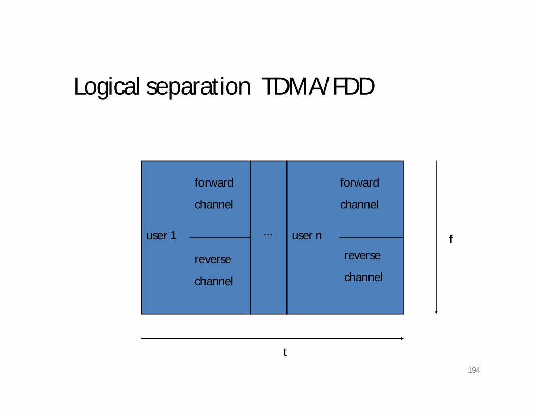
Logical separation TDMA/FDD
f
t
user 1 user n
forward
channel
reverse
channel
forward
channel
reverse
channel
...
194

Logical separation TDMA/TDD
f
t
user 1 user n
forward
channel
reverse
channel
forward
channel
reverse
channel
...
195

Wideband systems large number of transmitters on one channel TDMA techniques CDMA techniques FDD or TDD multiplexing techniques TDMA/FDD TDMA/TDD CDMA/FDD CDMA/TDD
196

Logical separation CDMA/FDD
code
f
user 1
user n
forward channel reverse channel
forward channel reverse channel
...
197

Logical separation CDMA/TDD
code
t
user 1
user n
forward channel reverse channel
forward channel reverse channel
...
198

Multiple Access Techniques in use
Multiple Access
TechniqueAdvanced Mobile Phone System (AMPS) FDMA/FDD
Global System for Mobile (GSM) TDMA/FDD
US Digital Cellular (USDC) TDMA/FDD
Digital European Cordless Telephone (DECT) FDMA/TDD
US Narrowband Spread Spectrum (IS-95) CDMA/FDD
Cellular System
199
Frequency division multiple access FDMA
One phone circuit per channel Idle time causes wasting of resources Simultaneously and continuously transmitting Usually implemented in narrowband systems For example: in AMPS is a FDMA bandwidth of 30 kHz implemented
200

FDMA compared to TDMA
Fewer bits for synchronization Fewer bits for framing Higher cell site system costs Higher costs for duplexer used in base station and subscriber units
FDMA requires RF filtering to minimize adjacent channel interference
201
Nonlinear Effects in FDMA
Many channels - same antenna For maximum power efficiency operate near saturation Near saturation power amplifiers are nonlinear Nonlinearities causes signal spreading Intermodulation frequencies
202

Nonlinear Effects in FDMA
IM are undesired harmonics Interference with other channels in the FDMA system Decreases user C/I - decreases performance Interference outside the mobile radio band: adjacent-channel interference RF filters needed - higher costs
203

Number of channels in a FDMA system
N … number of channels Bt … total spectrum allocation Bguard … guard band
Bc … channel bandwidth
N= Bt - Bguard
Bc
204

Time Division Multiple Access Time slots One user per slot Buffer and burst method Noncontinuous transmission Digital data
Digital modulation
205

Slot 1 Slot 2 Slot 3 … Slot N
Repeating Frame Structure
Preamble Information Message Trail Bits
One TDMA Frame
Trail Bits Sync. Bits Information Data Guard Bits
The frame is cyclically repeated over time.
206

Features of TDMA A single carrier frequency for several users Transmission in bursts Low battery consumption Handoff process much simpler FDD : switch instead of duplexer Very high transmission rate High synchronization overhead Guard slots necessary
207
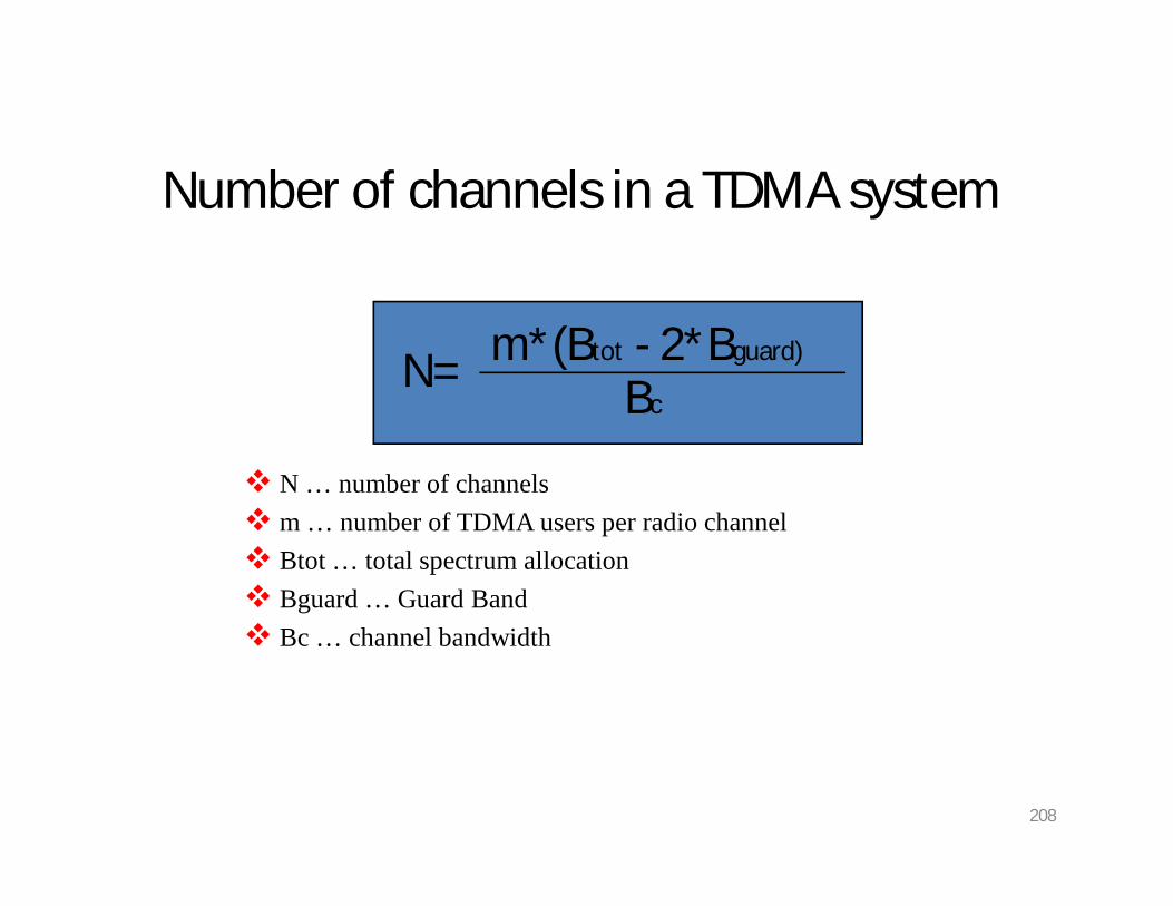
Number of channels in a TDMA system
N … number of channels m … number of TDMA users per radio channel Btot … total spectrum allocation Bguard … Guard Band Bc … channel bandwidth
N= m*(Btot - 2*Bguard)
Bc
208

Example: Global System for Mobile (GSM)
TDMA/FDD forward link at Btot = 25 MHz radio channels of Bc = 200 kHz if m = 8 speech channels supported, and if no guard band is assumed :
N= 8*25E6200E3 = 1000 simultaneous users
209

Efficiency of TDMA
Percentage of transmitted data that contain information Frame efficiency f Usually end user efficiency < f , Because of source and channel coding
210

Slot 1 Slot 2 Slot 3 … Slot N
Repeating Frame Structure
Preamble Information Message Trail Bits
One TDMA Frame
Trail Bits Sync. Bits Information Data Guard Bits
The frame is cyclically repeated over time.
211

Efficiency of TDMA
bOH … number of overhead bits Nr … number of reference bursts per frame br … reference bits per reference burst Nt … number of traffic bursts per frame bp … overhead bits per preamble in each slot bg … equivalent bits in each guard time intervall
bOH = Nr*br + Nt*bp + Nt*bg + Nr*bg
212

Efficiency of TDMA
bT … total number of bits per frame Tf … frame duration R … channel bit rate
bT = Tf * R
213

Efficiency of TDMA
f … frame efficiency bOH … number of overhead bits per frame bT … total number of bits per frame
f = (1-bOH/bT)*100%
214
Space Division Multiple Access
Controls radiated energy for each user in space using spot beam antennas base station tracks user when moving cover areas with same frequency: TDMA or CDMA systems cover areas with same frequency: FDMA systems
215

Space Division Multiple Access
primitive applications are “Sectorizedantennas”
In future adaptive antennas simultaneouslysteer energy in the direction of many users atonce
216

Reverse link problems
General problem Different propagation path from user to base Dynamic control of transmitting power from each user to the base station required Limits by battery consumption of subscriber units Possible solution is a filter for each user
217

Solution by SDMA systems
Adaptive antennas promise to mitigate reverse link problems Limiting case of infinitesimal beamwidth Limiting case of infinitely fast track ability Thereby unique channel that is free from interference All user communicate at same time using the same channel
218
Disadvantage of SDMA
Perfect adaptive antenna system: infinitely large antenna needed
Compromise needed
219

SDMA and PDMA in satellites
INTELSAT IVA
SDMA dual-beam receive antenna
Simultaneously access from two different regions of the earth
220

SDMA and PDMA in satellites
• COMSTAR 1• PDMA• separate antennas• simultaneously
access from same region
221

SDMA and PDMA in satellites
INTELSAT V
PDMA and SDMA
Two hemispheric coverage by SDMA
Two smaller beam zones by PDMA
Orthogonal polarization
222

Capacity of Cellular Systems
Channel capacity: maximum number of users in a fixed frequency band
Radio capacity : value for spectrum efficiency
Reverse channel interference
Forward channel interference
How determine the radio capacity?
223

Co-Channel Reuse Ratio Q
Q … co-channel reuse ratio
D … distance between two co-channel cells
R … cell radius
Q=D/R
224

Forward channel interference
cluster size of 4
D0 … distance serving station to user
DK … distance co-channel base station to user
225

Cellular Wireless Network Evolution
• First Generation: Analog– AMPS: Advance Mobile Phone Systems– Residential cordless phones
• Second Generation: Digital– IS-54: North American Standard - TDMA– IS-95: CDMA (Qualcomm)– GSM: Pan-European Digital Cellular– DECT: Digital European Cordless Telephone
226

Cellular Evolution (cont)• Third Generation: T/CDMA– combines the functions of: cellular, cordless, wireless LANs,
paging etc.– supports multimedia services (data, voice, video, image)– a progression of integrated, high performance systems:(a) GPRS (for GSM)(b) EDGE (for GSM)(c) 1xRTT (for CDMA)(d) UMTS
227

228

Invented by Bell Labs; installed In US in 1982; in Europe as TACS
229

AMPS (Advance Mobile Phone System):
In each cell, 57 channels each for A-side and B -side carrierrespectively; about 800 channels total (across the entire
AMPS system)
B
A
ED
C
F
G
B
A
ED
C
F
G
B
A
ED
C
F
G Frequency Reuse: Frequencies are not reused in a group of 7 adjacent cells
FDMA (Frequency Div Multiple Access): one frequencyper user channel
230

Advanced Mobile Phone System
(a) Frequencies are not reused in adjacent cells.(b) To add more users, smaller cells can be used.
231

Channel CategoriesThe channels are divided into four categories:
• Control (base to mobile) to manage the system
• Paging (base to mobile) to alert users to calls for them
• Access (bidirectional) for call setup and channel assignment
• Data (bidirectional) for voice, fax, or data
232

Handoff• Handoff: Transfer of a mobile from one cell to another• Each base station constantly monitors the received power
from each mobile.• When power drops below given threshold, base station
asks neighbor station (with stronger received power) to pick up the mobile, on a new channel.
• In APMS the handoff process takes about 300 msec.• Hard handoff: user must switch from one frequency to
another (noticeable disruption)• Soft Handoff (available only with CDMA): no change in
frequency.
233

To register and make a phone call
• When phone is switched on , it scans a preprogrammed list of 21 control channels, to find the most powerful signal.
• It transmits its ID number on it to the MSC – which informs the home MSC (registration is done every 15 min)
• To make a call, user transmits dest Ph # on random accesschannel; MSC will assign a data channel
• At the same time MSC pages the destination cell for the other party (idle phone listens on all page channels)
234

(Freq DivisionDuplex)
235

236

Digital Cellular: IS-54 TDMA System• Second generation: digital (as opposed to analog as in
AMPS)• Same frequency as AMPS• Each 30 kHz RF channel is used at a rate of 48.6 kbps
– 6 TDM slots/RF band (2 slots per user)– 8 kbps voice coding– 16.2 kbps TDM digital channel (3 channels fit in 30kHz)
• 4 cell frequency reuse (instead of 7 as in AMPS)• Capacity increase per cell per carrier
– 3 x 416 / 4 = 312 (instead of 57 in AMPS)– Additional factor of two with speech activity detection.
237

238
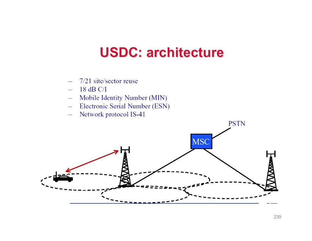
239

GSM (Group Speciale Mobile)Pan European Cellular StandardSecond Generation: DigitalFrequency Division Duplex (890-915 MHz Upstream; 935-960 MHz Downstream)125 frequency carriers
Carrier spacing: 200 Khz8 channels per carrier (Narrowband Time Division)
Speech coder: linear predictive coding (Source rate = 13 Kbps)
Modulation: phase shift keying (Gaussian minimum shift keying)
Slow frequency hopping to overcome multipath fading
240

241
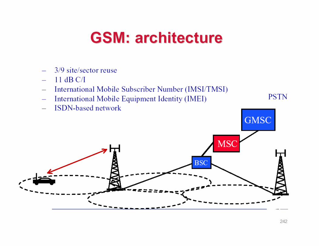
242

243
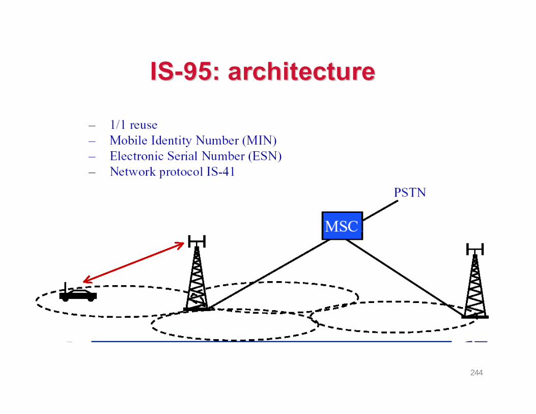
244