center for turbulence research annual research briefs … · equation 2.4 is unsolvable in the form...

Center for Turbulence ResearchAnnual Research Briefs 2012

179

Conservative volume of fluid advection method onunstructured grids in three dimensions

By C. B. Ivey AND P. Moin

1. Motivation and objectives

The volume of fluid (VOF) method is one of the most widely used formulations to trackinterfaces between two immiscible fluids in free-surface and interfacial flow simulations.In this method, the interface evolution is implicitly tracked using a discrete indicatorfunction, F , whose value represents the volume fraction of the tagged fluid within a cell.F is the cell average of the fluid marker function, f , that is constant in each phase andjumps at the interface from 0 to 1. As described by Scardovelli & Zaleski (1999), thevariations in VOF algorithms can be distinguished by the routines used to locate theimplicit interface and by the methods used to integrate the volume fraction equation intime, respectively known as the reconstruction and advection steps.

Of the VOF algorithms in use, the geometric formulations are more accurate than theiralgebraic counterparts, of which classic upwinding schemes come to mind. Traditionalfirst-order upwinding maintains the boundedness and globally conserves F ; however, itquickly smears out the interface. Higher-order upwinding schemes help maintain theintegrity of the interface; however, they lack boundedness in F , creating a whole slew ofproblems. The benefit of the algebraic methods are their simplicity; they do not requireany reconstruction of the interface.

Geometric algorithms locally approximate the interface with a lower-dimensional man-ifold, so that analytic techniques can be encompassed into the VOF method to helppreserve the integrity of the interface, while maintaining the local conservation of F . Aspecific class of the geometric algorithms that describe the interface by a series of dis-connected planes, named the piecewise-linear interface calculation (PLIC), has gainedpopularity within the VOF community for their great foundation of available geometrictools. As a side note, the nomenclature was developed during the era of two-dimensional(2D) VOF, hence the usage of “linear” in lieu of “planar”. Specifically, PLIC represen-tations allow for the use of analytic routines to determine the volume fraction in aninterface containing cell and to solve the inverse problem, placing the local interface suchthat a desired volume fraction is maintained; these procedures are integral to the recon-struction and advection steps. Scardovelli (2000) developed the tools for rectangular andhexahedral elements, Yang & James (2006) determined the analytics for triangular andtetrahedral meshes, and Lopez & Hernandez (2008) published the geometric operationsfor general convex grids.

PLIC-VOF can be further categorized by means of integration of the advection equa-tion. The integration can be split along each coordinate direction, or the equation can beintegrated all at once, irrespective of the coordinate direction. Split advection is muchsimpler to implement, but it has the added cost of requiring an advection and reconstruc-tion step for each dimension. Further, continuity is satisfied over the entire space, notalong a given direction, so divergence-based forcing terms need to be incorporated intothe formulation. Of the many directionally split schemes, Weymouth & Yue (2010) pro-

180 C. B. Ivey and P. Moin

posed the only one that discretely conserves volume. They cleverly introduced a modifieddivergence forcing term that ensured F remained bounded during each one-dimensional(1D) advection step and that the full advection sequence was conservative. Continuitycombined with volume conservation enforces density conservation, traditionally a zeroth-order constraint for any simulated system, due to the scaling of mass, momentum, andenergy fluxes on density. For liquid fuel combustion, a problem of particular interest tothe authors of this brief, the fuel density is typically three orders of magnitude largerthan that of the oxidizer, making local volume conservation paramount to simulationaccuracy.

Unsplit advection schemes do not have any source terms; however, the design of theadvection operator is complicated by the added dimensionality of the system. Inconve-niently, operator split schemes cannot be used within unstructured mesh environments,a necessary gridding paradigm for practical geometries, yielding unsplit advection algo-rithms as the only potential basis for realistic liquid fuel combustion simulations. Twoseminal works in this area deserve credit for their direct impact on the development of thescheme described herein, Lopez et al. (2004) and Hernandez et al. (2008). Both papersdescribed the use of flux polyhedra, a construct detailed in Section 2.1, to accuratelyevolve F in time; they quoted accuracies comparable to the top-of-the-line contempo-rary schemes, somewhere between first- and second-order. Lopez et al. (2004) describeda 2D algorithm that could conservatively advect F using edge-matched flux polyhedra(EMFPA-2D). Hernandez et al. (2008) described their three-dimensional (3D) extensionof EMFPA, the face-matched flux polyhedra (FMFPA-3D). Whereas EMFPA-2D, witha properly chosen time-step, could prevent the formation of over-/undershoots in thevolume fraction by discretely enforcing that the flux polyhedra do not over-/underlap,FMFPA-3D could only reduce the formation of over-/undershoots in the volume fraction.FMFPA-3D required the use of a volume fraction redistribution and/or flux rescaling al-gorithm; these are unphysical, zeroth-order corrections that destroy the accuracy of theVOF method. Hernandez et al. (2008) suggested that it would be possible to designan edge-matched flux polyhedra scheme in 3D (EMFPA-3D); however, they left that asa future development for the VOF community. The objective of this brief is to detailEMFPA-3D, an unsplit PLIC-VOF advection scheme that conservatively and accuratelyevolves F in time on an unstructured 3D mesh by ameliorating the aforementioned fluxpolyhedra construct.

2. EMFPA-3D

The equations governing the motion of an unsteady, viscous, incompressible, immisci-ble two-fluid system are the Navier-Stokes equations, augmented by a localized surfacetension force:

ρ

(

∂~v

∂t+ ~v · ∇~v

)

= −∇p + ∇ ·(

µ[

∇~v + ∇~vT])

+ ρ~g − σκΣδΣnΣ

∇ · ~v = 0,

(2.1)

where, ρ is the density, ~v is the velocity, p is the pressure, µ is the viscosity, ~g is thegravitational force, σ is the surface tension coefficient, Σ represents the interface, κΣ isthe surface curvature at the interface, δΣ is a delta function located at the interface, andnΣ is the surface normal at the interface. This one-fluid system of equations requiresknowledge of the interface location to determine ρ, µ, and the localized surface tension

Conservative VOF method on unstructured grids 181

force. A marker function, f , is used to implicitly track the interface. f is a Heavisidefunction that takes on a value of 1 in the tagged fluid and 0 otherwise, so ρ and µ havea simple one-to-one correspondence with f . Because f is a passive tracer, it follows alinear advection equation:

∂f

∂t+ ~v · ∇f = 0. (2.2)

Integration of the above equation over the cell, Ω, and between the time interval, t′ǫ [t, t + ∆t],yields an equation for the cell volume fraction, F :

F (t + ∆t) = F (t) −1

VΩ

∫ t+∆t

t

∫

Ω

~v · ∇fdV dt′. (2.3)

Utilization of the continuity condition in conjunction with the divergence theorem alonga surface, S, leads to a simple, flux-based update rule for F :

F (t + ∆t) = F (t) −1

VΩ

∫ t+∆t

t

∫

S

(~vf) · nAdAdt′. (2.4)

Equation 2.4 is unsolvable in the form above, with F still dependent on f . The VOFalgorithms essentially differ in how the flux term is discretized. This brief will describethe EMFPA-3D discretization developed at the Center for Turbulence Research (CTR).Before beginning the description of EMFPA-3D, certain assumptions need to be men-tioned. EMFPA-3D is a class of PLIC-VOF algorithms, so it requires a reconstructionstep to describe the interface locally as a plane, nΓc

· ~x + CΓc= 0, where Γ designates a

plane and c is the index of the plane. This notation is to be used later and is repeatedhere for consistency. The reconstruction step is not the focus of this brief, so the usage ofan acceptable estimator of nΓc

is assumed. In order for the scheme to be convergent, theestimation of the normal needs to be at least first-order accurate on general grids; thegradient-based approximation in Parker & Youngs (1992) fits this criterion, for example.Their method essentially calculates the gradient of F at the nodes surrounding the celland then averages those gradients to get a cell-averaged gradient. The gradient is thennegated and normalized to provide an estimation of nΓc

, which points into the referencefluid. The method uses more information than the traditional central differences to helpcharacterize sub-cell discontinuities. It should be emphasized that a second-order estima-tion of the normal would augment the total accuracy of the scheme, due to the empiricalaccuracy of the flux polyhedron, so the development of such a reconstruction is in theworks, namely mapping the height-functions described in Weymouth & Yue (2010) togeneral grids. CΓc

is determined using the volume enforcement procedure proposed inLopez & Hernandez (2008). Note that the volume enforcement procedure is integral to theconstruction of the flux polyhedron as well, so a more detailed derivation of the methodis provided in Section 2.1.1. The local surface curvature, κΓc

, is not needed to advect F ,so its estimation is left out of the brief. EMFPA-3D requires a solenoidal velocity fieldlocated at the faces of the mesh, limiting the use of the scheme to finite volume methods.Discrete continuity is necessary for the scheme to remain conservative; this is obviatedby the usage of the continuity condition above to get Eq. (2.4) in a flux formulation. Itis also assumed that there is only one face separating two cells; localized refinement withhanging nodes is not yet handled.

The EMFPA-3D algorithm breaks down the advection operator into a series of localadvection steps performed using flux polyhedra. The flux polyhedron is based on theidea of a stream tube, wherein the flux face is swept over a volume defined by the local


velocities and time step. There are many details involved in the construction of a fluxpolyhedron, due to the restriction of volume conservation and planar geometries; however,the geometric description aims to approximate the simple concept of a stream tube usingthe information available. The proposed advection algorithm is outlined below:

(a)Use distance-weighted averaging to interpolate the velocities from the faces to theirrespective adjacent nodes.

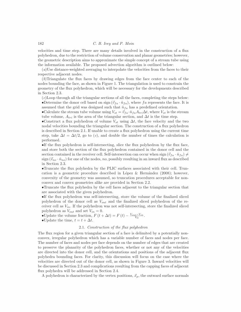
(b)Triangulate the flux faces by drawing edges from the face center to each of thenodes bounding the face, as shown in Figure 1. The triangulation is used to constrain thegeometry of the flux polyhedron, which will be necessary for the developments describedin Section 2.3.

(c)Loop through all the triangular sections of all the faces, completing the steps below:•Determine the donor cell based on sign (~vfa · nfa), where fa represents the face. It isassumed that the grid was designed such that nfa has a predefined orientation.•Calculate the stream tube volume using Vst = ~vfa ·nfaAtri∆t, where Vst is the streamtube volume, Atri is the area of the triangular section, and ∆t is the time step.•Construct a flux polyhedron of volume Vst using ∆t, the face velocity and the twonodal velocities bounding the triangular section. The construction of a flux polyhedronis described in Section 2.1. If unable to create a flux polyhedron using the current timestep, take ∆t = ∆t/2, go to (c), and double the number of times the calculation isperformed.•If the flux polyhedron is self-intersecting, slice the flux polyhedron by the flux face,and store both the section of the flux polyhedron contained in the donor cell and thesection contained in the receiver cell. Self-intersection can occur when sign (~vfa · nfa) 6=sign (~vno · nno) for one of the nodes, no, possibly resulting in an inward flux as describedin Section 2.3.•Truncate the flux polyhedra by the PLIC surfaces associated with their cell. Trun-cation is a geometric procedure described in Lopez & Hernandez (2008); however,convexity of the geometry was assumed, so truncation procedures acceptable for non-convex and convex geometries alike are provided in Section 2.2.•Truncate the flux polyhedra by the cell faces adjacent to the triangular section thatare associated with the given polyhedron.•If the flux polyhedron was self-intersecting, store the volume of the finalized slicedpolyhedron of the donor cell as Vout and the finalized sliced polyhedron of the re-ceiver cell as Vin. If the polyhedron was not self-intersecting, store the finalized slicedpolyhedron as Vout and set Vin = 0.•Update the volume fraction, F (t + ∆t) = F (t) − Vout−Vin

VΩ.

•Update the time, t = t + ∆t.

2.1. Construction of the flux polyhedron

The flux region for a given triangular section of a face is delimited by a potentially non-convex, irregular polyhedron which has a variable number of faces and nodes per face.The number of faces and nodes per face depends on the number of edges that are createdto preserve the planarity of the polyhedron faces, whether or not any of the velocitiesare directed into the donor cell, and the orientations and positions of the adjacent fluxpolyhedra bounding faces. For clarity, this discussion will focus on the case where thevelocities are directed out of the donor cell, as shown in Figure 3. Inward velocities willbe discussed in Section 2.3 and complications resulting from the capping faces of adjacentflux polyhedra will be addressed in Section 2.4.

A polyhedron is characterized by the vertex positions, ~xp, the outward surface normals


Figure 1. Triangulation of the flux face en-ables the algorithm to handle self-intersectionof the flux polyhedron by constraining the ge-ometry.

fa

nfaδ

cv

Figure 2. Use distance between face and cellcenter in the normal direction as length scalefor creating planarity-preserving edges.

ec,2

ec,1

ec,3

ec,4

ec,5

ec,0

v0

v1

v2

00 0

1

1

2

2

2

Figure 3. Edges bounding stream tube are acombination of vectors anti-parallel to the ve-locity vectors and the vectors created to pre-serve planarity.

v0

v1

v2

00 0

1

1

2

2

2

3

4

5

6

7

8Γ0Γ1

Γ2

Γ3

Γ4

Γ5

Γ6

Γ7

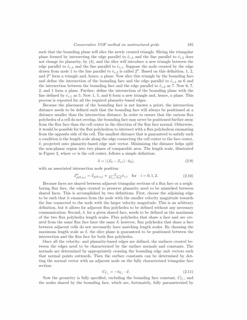
Figure 4. Placement of plane such that thevolume bound by the flux polyhedron equalsthat of the flux through the triangular face sec-tion, Vst.

and constants, nΓjand CΓj

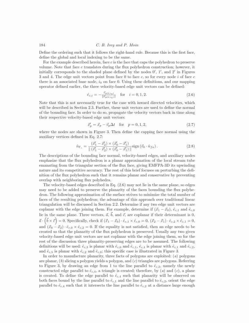
, and the mapping from the global node index to the localnode index for a given surface, p (j, i), where the local indices follow a right-hand rulearound the outward normal of the face. For clarity, p will be used solely for global nodeindexing, j for face indexing, and i for local face indexing. This information is required forany and all geometric operations to be performed on the flux polyhedron. The descriptionprovided herein will follow the example fully detailed in Figures 3 and 4. The procedureis quite general; however, the specificity allows for a simpler description.

First, fully characterize the triangular flux face section, face 0 in this example. Thenodal positions, ~xp, and velocities, ~vp, are provided for p = 0, 1, 2. The respective normaldepends on which cell is the donor cell:

n0 = nfasign (~v0 · nfa) . (2.5)


Define the ordering such that it follows the right-hand rule. Because this is the first face,define the global and local indexing to be the same.

For the example described herein, face c is the face that caps the polyhedron to preservevolume. Note that face c translates during the flux polyhedron construction; however, itinitially corresponds to the shaded plane defined by the nodes 0′, 1′, and 2′ in Figures3 and 4. The edge unit vectors point from face 0 to face c, so for every node i of face cthere is an associated base node, i0 on face 0. Using these definitions, and our mappingoperator defined earlier, the three velocity-based edge unit vectors can be defined:

ec,i = −~vp(0,i0)

‖~vp(0,i0)‖for i = 0, 1, 2. (2.6)

Note that this is not necessarily true for the case with inward directed velocities, whichwill be described in Section 2.3. Further, these unit vectors are used to define the normalof the bounding face. In order to do so, propagate the velocity vectors back in time alongtheir respective velocity-based edge unit vectors:

~x′p = ~xp − ~vp∆t for p = 0, 1, 2, (2.7)

where the nodes are shown in Figure 3. Then define the capping face normal using theauxiliary vertices defined in Eq. 2.7:

nΓc=

(~x′1 − ~x′

2) × (~x′0 − ~x′

1)

‖ (~x′1 − ~x′

2) × (~x′0 − ~x′

1) ‖sign (~v0 · nfa) . (2.8)

The descriptions of the bounding face normal, velocity-based edges, and auxiliary nodesemphasize that the flux polyhedron is a planar approximation of the local stream tubeemanating from the triangular section of the flux face, giving EMFPA-3D its upwindingnature and its competitive accuracy. The rest of this brief focuses on perturbing the defi-nition of the flux polyhedron such that it remains planar and conservative by preventingoverlap with neighboring flux polyhedra.

The velocity-based edges described in Eq. (2.6) may not lie in the same plane, so edgesmay need to be added to preserve the planarity of the faces bounding the flux polyhe-dron. The following approximation of the surface strives to minimize the total number offaces of the resulting polyhedron; the advantage of this approach over traditional lineartriangulation will be discussed in Section 2.2. Determine if any two edge unit vectors arecoplanar with the edge joining them. For example, determine if (~x1 − ~x0), ec,1 and ec,0

lie in the same plane. Three vectors, ~a, ~b, and ~c, are coplanar if their determinant is 0,

~a ·(

~b × ~c)

= 0. Specifically, check if (~x1 − ~x0) · ec,1 × ec,0 = 0, (~x2 − ~x1) · ec,2 × ec,1 = 0,

and (~x0 − ~x2) · ec,0 × ec,2 = 0. If the equality is not satisfied, then an edge needs to becreated so that the planarity of the flux polyhedron is preserved. Usually any two givenvelocity-based edge unit vectors are not coplanar with the edge joining them, so for therest of the discussion three planarity-preserving edges are to be assumed. The followingdefinitions will be used: ec,3 is planar with ec,0 and ec,1, ec,4 is planar with ec,1 and ec,2,and ec,5 is planar with ec,2 and ec,0; this specific case is illustrated in Figure 3.

In order to manufacture planarity, three facts of polygons are exploited: (a) polygonsare planar, (b) slicing a polygon yields a polygon, and (c) triangles are polygons. Referringto Figure 3, by drawing an edge from 1 to the line parallel to ec,2, namely the newlyconstructed edge parallel to ec,4, a triangle is created; therefore, by (a) and (c), a planeis created. To define the edge parallel to ec,4 such that planarity will be observed onboth faces bound by the line parallel to ec,1 and the line parallel to ec,2, orient the edgeparallel to ec,4 such that it intersects the line parallel to ec,2 at a distance large enough


such that the bounding plane will slice the newly created triangle. Slicing the triangularplane formed by intersecting the edge parallel to ec,4 and the line parallel to ec,2 doesnot change its planarity, by (b), and the slice will introduce a new triangle between theedge parallel to ec,4 and the line parallel to ec,1. Suppose the node created by the edgedrawn from node 1 to the line parallel to ec,2 is called 2′′. Based on this definition, 1, 2,and 2′′ form a triangle and, hence, a plane. Now slice this triangle by the bounding faceand define the intersection of the bounding face and the edge parallel to ec,4 as 6 andthe intersection between the bounding face and the edge parallel to ec,2 as 7. Now 6, 7,2, and 1 form a plane. Further, define the intersection of the bounding plane with theline defined by ec,1 as 5. Now 1, 5, and 6 form a new triangle and, hence, a plane. Thisprocess is repeated for all the required planarity-based edges.

Because the placement of the bounding face is not known a priori, the intersectiondistance needs to be defined such that the bounding face will always be positioned at adistance smaller than the intersection distance. In order to ensure that the various fluxpolyhedra of a cell do not overlap, the bounding face may never be positioned further awayfrom the flux face than the cell center in the direction of the flux face normal. Otherwise,it would be possible for the flux polyhedron to intersect with a flux polyhedron emanatingfrom the opposite side of the cell. The smallest distance that is guaranteed to satisfy sucha condition is the length scale along the edge connecting the cell center to the face center,δ, projected onto planarity-based edge unit vector. Minimizing the distance helps splitthe non-planar region into two planes of comparable area. The length scale, illustratedin Figure 2, where cv is the cell center, follows a simple definition:

δ = | (~x0 − ~xcv) · n0|, (2.9)

with an associated intersection node position:

~x′′p(0,i0)

= ~xp(0,i0) + δ‖ec,i·n0‖

ec,i for i = 0, 1, 2. (2.10)

Because faces are shared between adjacent triangular sections of a flux face or a neigh-boring flux face, the edges created to preserve planarity need to be mimicked betweenshared faces. This is accomplished by two definitions. First, choose the adjoining edgeto be such that it emanates from the node with the smaller velocity magnitude towardsthe line connected to the node with the larger velocity magnitude. This is an arbitrarydefinition, but it allows for adjacent flux polyhedra to be defined without any necessarycommunication. Second, δ, for a given shared face, needs to be defined as the maximumof the two flux polyhedra length scales. Flux polyhedra that share a face and are cre-ated from the same flux face have the same δ; however, flux polyhedra that share a facebetween adjacent cells do not necessarily have matching length scales. By choosing themaximum length scale as δ, the slice plane is guaranteed to be positioned between theintersection and the flux face for both flux polyhedra.

Once all the velocity- and planarity-based edges are defined, the surfaces created be-tween the edges need to be characterized by the surface normals and constants. Thenormals are determined by appropriately crossing the bounding edge unit vectors suchthat normal points outwards. Then the surface constants can be determined by dot-ting the normal vector with an adjacent node on the fully characterized triangular facesection:

CΓj= −nΓj

· ~x. (2.11)

Now the geometry is fully specified, excluding the bounding face constant, CΓc, and

the nodes shared by the bounding face, which are, fortunately, fully parameterized by


CΓc. This parameterization is based on a fixed capping face normal, nΓc

. CΓcwill shift

the bounding plane to enforce the flux polyhedron volume to be Vst. There are associ-ated min and max limits on the allowable CΓc

in order to prevent the polyhedron fromextruding beyond the bounds set by the cell center and flux face; if a polyhedron cannotbe constructed such that the volume matching occurs, the advection procedure muststart over using a smaller time step, as outlined in Section 2. As a side note, nΓc

wasspecified using Eq. (2.7), so the orientation implicitly had a velocity dependence; shiftingthe plane with a fixed normal does not respect this velocity dependence. If a shift inthe capping plane is envisaged as a respective increase or decrease in time, the volumeenforcement procedure can further respect the stream tube idealization. Another volumeenforcement procedure can be defined with an orientable and shiftable capping surface,where the parameterization with CΓc

is augmented by the definitions in Eq. (2.7). Thisprocedure is left out of the brief as it has not yet been fully formulated.

2.1.1. Determination of bounding face position

The volume of a polyhedron can be determined by the surface normals and vertexpositions, where j is the face index, i is the local node index, Ij is the number of nodesin face j, and J is the number of faces. Periodicity in i is assumed:

6Vst =

J−1∑

j=0

(

nΓj· ~xj,0

)

nΓj·

Ij−1∑

i=0

(~xj,i × ~xj,i+1)

= −

J−1∑

j=0

Ij−1∑

i=0

(~xj,i × ~xj,i+1) · nΓjCΓj

.

(2.12)Split off the slicing plane from the equation:

6Vst = −

Ic−1∑

i=0

(~xc,i × ~xc,i+1) · nΓcCΓc

−J−1∑

j=0j 6=c

Ij−1∑

i=0


. (2.13)

Define the unknown polyhedron node cut by the plane, ~xc,i, by the slope of the plane,nΓc

, the direction of the cut edge, ec,i, and the associated node along the edge locatedon the flux face, ~x0,i0 . ec,i and ~x0,i0 were determined earlier during the construction ofthe flux polyhedron:

~x0c,i = ~x0,i0 −

nΓc· ~x0,i0

nΓc· ec,i

ec,i = ~x0,i0 + βc,inΓc· ~x0,i0 ec,i

~xc,i = ~x0c,i −

CΓc

nΓc· ec,i

ec,i = ~x0c,i + βc,iCΓc

ec,i.

(2.14)

Substitute the parameterization in Eq. (2.14) and simplify:

Ic−1∑

i=0


=

Ic−1∑

i=0

(ec,i × ec,i+1) βc,i+1βc,i · nΓcC3

Γc

+

Ic−1∑

i=0

[

ec,i ×(

~x0c,i+1 − ~x0

c,i−1

)]

βc,i · nΓcC2

Γc

+

Ic−1∑

i=0

(

~x0c,i × ~x0

c,i+1

)

· nΓcCΓc

.

(2.15)


Rewrite the equation using the following terms: ~MΓc=

∑Ic−1i=0 (ec,i × ec,i+1) βc,iβc,i+1,

~LΓc=

∑Ic−1i=0

[

ec,i ×(

~x0c,i−1 − ~x0

c,i+1

)]

βc,i, and ~KΓc=

∑Ic−1i=0

(

~x0c,i × ~x0

c,i+1

)

:

Ic−1∑

i=0


= ~MΓc· nΓc

C3Γc

+ ~LΓc· nΓc

C2Γc

+ ~KΓc· nΓc

CΓc. (2.16)

Recognize that face j can be parameterized exactly as c, xj,i = x0j,i +βj,iCΓj

ej,i, where

ej,i = 0, βj,i = 0, and x0j,i = xj,i when i is not an adjoining node of face c. Then recognize

that for j 6= c, faces will have one less power in CΓcthan face c:

Ij−1∑

i=0


= ~MΓj· nΓj

CΓjC2

Γc+ ~LΓj

· nΓjCΓj

CΓc+ ~KΓj

· nΓjCΓj

. (2.17)

After substituting the parameterizations and the known terms, a cubic equation isrevealed, the solution of which positions the bounding plane, CΓc

:

6Vst = α3C3Γc

+ α2C2Γc

+ α1CΓc+ α0, (2.18)

where α3 = − ~MΓc· nΓc

, α2 = −~LΓc· nΓc

−∑J−1

j=0,j 6=c~MΓj

· nΓjCΓj

,

α1 = − ~KΓc· nΓc

−∑J−1

j=0,j 6=c~LΓj

· nΓjCΓj

, and α0 = −∑J−1

j=0,j 6=c~KΓj

· nΓjCΓj

. SubstituteCΓc

into the parameterization of Eq. (2.14) for the unknown node positions to full specifythe flux polyhedron, as shown in Figure 4.

2.2. Truncation of the flux polyhedron

Because only the tagged volume is tracked, the flux polyhedron should be truncated bythe PLIC surface. Further, in order to prevent overlap between adjacent cells sharing acommon edge, the flux polyhedron needs to be truncated by the donor cell faces thatare adjacent to the flux face. The resulting flux polyhedron volume is donated from thedonor to the receiver cell, completing the local advection step. Truncation procedures aredescribed in Lopez & Hernandez (2008), the details of which are repeated here becausea clarification needs to be made in regards to the non-convexity of the flux polyhedron.

Calculate the signed distance, φp, from every vertex, ~xp, to the truncation plane, T ,using φp = nΓT

· ~xp + CΓT. An edge is defined to be intersected if the relative signs of φ

for the two nodes bounding the edge change sign. The distance functions can be used tolocate the intersected points. For example, if an intersected edge is bound by ~x1 and ~x2,the intersection position can be found using ~xt = ~x1 − φ1

φ2−φ1(~x2 − ~x1), where t is the

index of the node created by the intersection.The truncation procedure removes the nodes with a negative φ and use the the vertices

with positive φ and the intersected nodes to build up the truncated polyhedron. Due tothe non-convexity of the flux region, the truncation procedure can slice the polyhedron inmultiple sections, introducing multiple new faces to the polyhedron, or, possibly, creat-ing multiple polyhedra. Because the non-convexity of the flux region is restricted to twoadjacent planes, created by the added planarity-preserving edge between two velocityedges, the truncation procedure can introduce up to two new faces to the polyhedronor separate the polyhedron into two polyhedra. In order to use convex truncation pro-cedures, the polyhedron is broken up into a set of convex tetrahedra for the duration ofthe operation. Nevertheless, because the non-convexity is mild, the truncation procedureusually operates as if the polyhedron is convex, as shown by in Figures 5-7. The trunca-tion step is costly relative to the rest of the algorithm, so the number of reconstructed


Figure 5. Truncation of the flux polyhedronby the top face.

Figure 6. Truncation of the flux polyhedronby the back face.

Figure 7. Truncation of the polyhedron by thePLIC plane. Shaded region volume is donatedto the receiver cell.

tetrahedra should be minimized; this is accomplished by minimizing the number of sur-faces bounding the non-convex polyhedron. Linear triangulation of a non-planar surfaceproduces more flux polyhedron faces than the procedure described in Section 2.1.

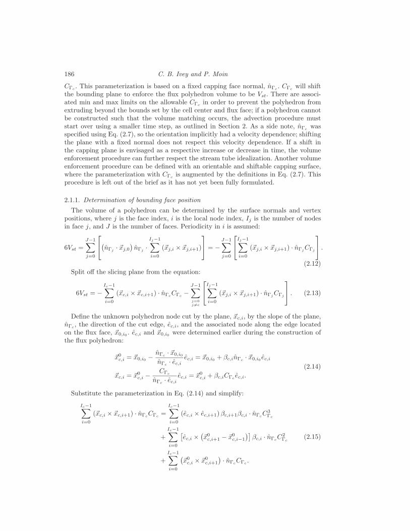
2.3. Handling of inward velocities

If there exists a node where sign (~vfa · nfa) 6= sign (~vno · nno), then there is an inwardvelocity. Inward velocities have the potential to create a self-intersecting flux polyhedron,where some of the resulting flux will be be donated from the receiver cell to the donor cell.We can only determine whether the inward velocity has caused the flux polyhedron to beself-intersecting once we have tried to place the bounding face to match the stream tubevolume. Essentially, if the assumption of self-intersection does not permit a placementof the bounding face such that stream tube volume is matched, then it is not self-intersecting. So, first assume the inward velocity makes the polyhedron self-intersecting


v1

v0

v2

ec,1

ec,0

ec,2

ec,3

00 0

2

2

1

1

Figure 8. Self-intersecting case has veloci-ty-based edges propagate in both directions.Note that a planarity edge is not needed be-tween nodes with velocities in opposing direc-tions.

v1

v0

v2

00 0

2

2

1

1

7

6

5

4

3

8

Γ0

Γ1

Γ2

Γ3

Γ4

Γ5

Γ6Γ7

Figure 9. The self-intersecting has thecapping plane slice the flux face.

Figure 10. The self-intersected flux polyhe-dron has both positive and negative fluxed vol-ume.

and define the geometry as such. If the plane cannot be placed in such a way that itslices the flux face, then the situation reverts to a case where all the flux is outward andthe geometry is defined by the traditional method described above.

The self-intersecting case is systematically constructed in Figures 8-10. The programis essentially the same as the one described above. The only caveat is that there is noneed to add planarity-preserving edges to the regions between the nodes that have theirvelocities pointing in opposite directions; instead, the edges are constrained such thatthey connect to an edge bounding the triangular flux face section to preserve planarity.This behavior is illustrated in Figure 9 by nodes 6 and 8. Note that the auxiliary nodesused to define the normal of bounding plane still follow the relation, ~x′

p = ~xp − ~vp∆t;however, this definition causes one of the nodes to propagate into the receiving cell. Also,because the volume is negative, all normals for the faces living in the receiving cell, andthe associated local indices, need to be reversed to use Eq. (2.12) and (2.18). Note thatthe bounding plane is considered as one face in this definition and its normal still pointsoutward. If there is a negative volume region, truncation operations for the cell faces andthe PLIC planes need to be performed for both the donor and receiver cell. Further, ifthere are two inward velocities that are non-planar, the planarity-based edges need to bedefined using the maximum length scale defined by the receiver cell and the associatedface adjacent neighbor.


v1

v2

v0

2

2

00

1

0

1

2

ec,0

ec,1

ec,2

ec,3

ec,4

ec,5

Figure 11. Non-intersecting case has the ve-locity-based edge of the inward velocity flippedbecause the volume could not be conservedwith self-intersection.

v1

v2

v0

Γ0Γ1

Γ2

Γ3

Γ4

Γ5

Γ6

Γ7

2

2

00

1

3

4

5

6

7

8

0

1

2

Figure 12. In the non-intersecting case, theplane does not slice the flux face even thoughthere was an inward velocity

Figure 13. The non-intersected fluxpolyhedron has only positive fluxed volume..

As mentioned above, if the self-intersecting geometry does not permit placement ofthe capping plane under the limits on CΓc

, defined by the flux face nodes and cell centerpositions, then the flux polyhedron falls back to the traditional description above, wheremore edges need to be added for planarity. The only difference is that the edge unitvector for the inward velocity is parallel to velocity vector, instead of anti-parallel. This isillustrated by ec,1 in Figure 11. The normal of the bounding face has the same orientationas if it were self-intersecting; however, the flux polyhedron in Figure 13 is geometricallysimilar to that in Figure 4.

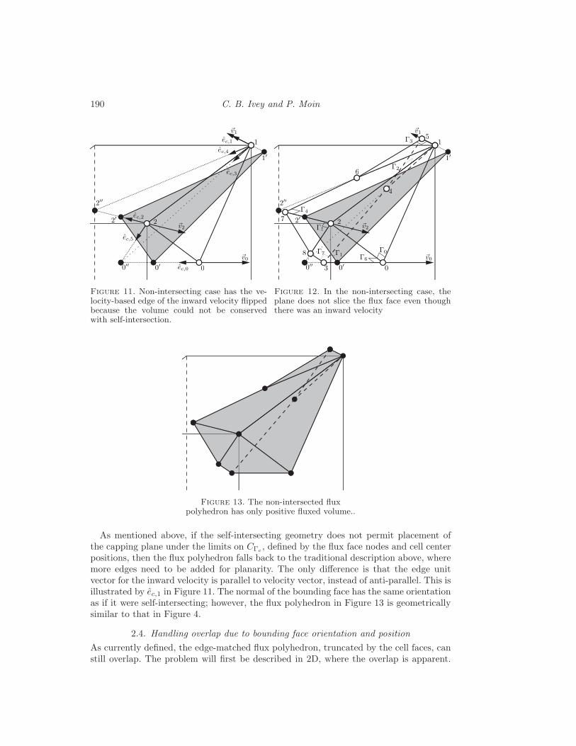
2.4. Handling overlap due to bounding face orientation and position

As currently defined, the edge-matched flux polyhedron, truncated by the cell faces, canstill overlap. The problem will first be described in 2D, where the overlap is apparent.


0

1

2

34

5

6 7

v0

v1

v2

Figure 14. 2D schematic of the overlapbetween adjacent flux polyhedra.

0

1

2

34

5

6 7

v0

v1

v2

7

4

Figure 15. 2D schematic of the corrected fluxpolyhedra to prevent overlap.

Note that in a 2D description, faces are replaced by edges. Following the 2D schematicin Figure 14, the flux polyhedron defined by the nodes 0, 2, 3, and 1 overlap with theadjacent flux polyhedron defined by nodes 4, 2, 6, and 7 over the region bound bynodes 3, 4, and 5. This overlap can be easily accounted for in the volume enforcementprocedure described in Section 2.1.1 by storing and using the bounding edge normaland constant from the antecedently reconstructed flux polyhedra of the cell. Figure 15illustrates the correction for the case where the flux polyhedron emanating from the topface is reconstructed first, so that the flux polyhedron emanating from the left face ismodified. The flux polyhedron originally defined by nodes 4, 2, 6, and 7 conservativelydeforms such that it is bound by nodes 4′, 3, 2, 6 and 7′. Basically the edge bound bynodes 2 and 3 is added to the left face flux polyhedron and the volume enforcementprocedure is repeated, using the bounding edge of the top face flux polyhedron, parallelto the edge bound by nodes 3 and 1, as the direction of propagation in lieu of the edgeanti-parallel to ~v1. The procedure is repeated for all subsequent flux polyhedra of thecell, namely from the bottom and right faces.

The procedures are very similar in 3D; however, the description is convoluted by theaddition of planarity-preserving faces. Store the antecedently reconstructed flux polyhe-dra bounding surface normals and constants of the cell. If during the volume enforcementprocedure, the subsequently reconstructed flux polyhedron’s bounding surface intersectsan adjacent polyhedron’s bounding surface, copy the face(s) shared by the adjacent fluxpolyhedron, bound by the two respective velocity-based edges, potentially the planarity-based edge, and the edge shared with the antecedently reconstructed flux polyhedron’scapping face, into the subsequently reconstructed flux polyhedron. This is equivalentto adding the edge defined by nodes 2 and 3 in the 2D description of Figure 15. Thenrepeat the volume enforcement procedure, replacing the propagation path defined byvelocity-based edges and potentially the planarity-based edge with an edge parallel tothe antecedently reconstructed flux polyhedron’s bounding face. This is equivalent to thedirection defined by the edge bound by nodes 3 and 1 in the 2D description of Figure15. Repeat for all subsequently reconstructed flux polyhedra of the cell.


3. Concluding remarks and future work

This brief describes a new PLIC-VOF advection method on general grids in 3D. Themethod formally conserves the local volume and has an empirical accuracy between first-and second-order. The method uses the flux polyhedron construct to locally approximatea stream tube emanating from the flux face, perturbing the definition in order to removeall over-/underlap to prevent the volume fraction from over-/undershooting. Kinematictest cases on unstructured grids have been performed; the results of the study, includ-ing estimation of cost and accuracy in comparison to contemporary algorithms, will beincluded in a future publication.

Future research will include: incorporation of EMFPA-3D into the mass and momen-tum advection operators in an incompressible Navier-Stokes solver that uses a node-basedfinite volume method, estimation of the surface normal and curvature on unstructuredgrids using height functions, augmentation of the volume enforcement procedure to havean orientable and shiftable capping surface, and incorporation of hanging nodes.

Acknowledgements

This work was supported by the Department of Energy Computational Science Gradu-ate Fellowship under grant number DE-FG02-97ER25308 and by the Stanford GraduateFellowship. The authors wish to thank Sanjeeb Bose, Paul Covington, Olivier Desjardins,Frank Ham, and Vincent Le Chenadec for their helpful discussions during the develop-ment of EMFPA-3D.

REFERENCES

Hernandez, J., Lopez, J., Gomez, P., Zanzi, C. & Faura, F. 2008 A new volumeof fluid method in three dimensions – Part I: Multidimensional advection methodwith face-matched flux polyhedra. Int. J. Numer. Meth. Fluids 58, 897–921.

Lopez, J. & Hernandez, J. 2008 Analytical and geometrical tools for 3D volume offluid methods in general grids. J. Comput. Physics 227, 5939–5948.

Lopez, J., Hernandez, J., Gomez, P. & Faura, F. 2004 A volume of fluid methodbased on multidimensional advection and spline interface reconstruction. J. Comput.

Physics 195, 718–742.

Parker, B. J. & Youngs, D. L. 1992 Two and three dimensional Eulerian simulationand fluid flow with material interfaces. Tech. Rep. 01/92. AWE.

Scardovelli, R. 2000 Analytical relations connecting linear interfaces and volume frac-tions in rectangular grids. J. Comput. Physics 164, 228–237.

Scardovelli, R. & Zaleski, S. 1999 Direct Numerical Simulation of free-surface andinterfacial flow. Annu. Rev. Fluid Mech. 31, 567–603.

Weymouth, G. D. & Yue, D. K. P. 2010 Conservative Volume-of-Fluid method forfree-surface simulations on Cartesian-grids. J. Comput. Physics 229, 2853–2865.

Yang, X. & James, A. J. 2006 Analytic relations for reconstructing piecewise linearinterfaces in triangular and tetrahedral grids. J. Comput. Physics 214, 41–54.

center for turbulence research annual research briefs … · equation 2.4 is unsolvable in the form...

Documents