centralized routing for prolonged network lifetime in wireless

Mälardalen University Licentiate ThesisNo.79

Centralized Routing forProlonged Network Lifetime in

Wireless Sensor Networks

Ewa Hansen

January 2008

School of Innovation, Design and EngineeringMälardalen University

Västerås, Sweden

Copyright c© Ewa Hansen, 2008ISSN 1651-9256ISBN 978-91-85485-69-7Printed by Arkitektkopia, Västerås, SwedenDistribution: Mälardalen University Press

Abstract

In this thesis centralized routing methods for wireless sensor networks havebeen studied. The aim has been to prolong network lifetime by reducing theenergy consumed by sensor-node communication.

Wireless sensor networks are rapidly becoming common in application ar-eas where information from many sensors is to be collected and acted upon.The use of wireless sensor networks adds flexibility to the network, and thecost of cabling can be avoided.

Wireless sensor networks may consist of hundreds or even up to thousandsof small compact devices, equipped with sensors (e.g. acoustic, seismic or im-age), that form a wireless network. Each sensor node in the network collectsinformation from its surroundings and sends it to a base station, either fromsensor node to sensor node, i.e. multihop, or directly to the base station i.e.,singlehop.

We have made simulations that show that asymmetric communication withmultihop extends the lifetime of large wireless sensor networks. We have alsoinvestigated the usefulness of enforcing a minimum separation distance be-tween cluster heads in a cluster based wireless sensor network. The resultsshow that our wireless sensor network performs up to 150% better when intro-ducing a minimum separation distance between cluster heads. The simulationsalso show that the minimum separation distance resulting in the lowest energyconsumption in our network varies with the number of clusters. Furthermorewe have made an initial study of maximum lifetime routing in sparse wirelesssensor networks to be able to see how different heuristic routing algorithmsinfluence the energy consumption of individual sensor nodes, and thus the life-time of a sparse sensor network. We have compared the maximum lifetime ofthe heuristic algorithms to the maximum lifetime of an optimal routing solu-tion. These simulations show that for some types of applications the choiceof heuristic algorithm is more important to prolong network lifetime than forother types of applications.

i

Swedish Summary - SvenskSammanfattning

I denna avhandling har centraliserade vägvalsmetoder för trådlösa sensornätverkstuderats. Målet har varit att förlänga nätverkens livslängd genom att minskaenergiåtgången för sensornodernas kommunikation.

Trådlösa sensornätverk blir en allt vanligare tillämpning där informationfrån många sensorer behöver samlas in och bearbetas. Användandet av trådlösasensornätverk ökar nätverkets flexibilitet, och kostnader för kabeldragning kanundvikas.

Trådlösa sensornätverk kan bestå av hundratals eller ända upp till tusentalssmå enheter, utrustade med en eller flera sensorer (för t.ex. ljud, ljus, rörelseeller bild), som formar ett trådlöst nätverk. Varje sensornod i nätverket samlarinformation från sin omgivning som den sedan skickar till basstationen antin-gen från sensornod till sensornod, s.k. multihop, eller direkt till basstationen,s.k. singelhop.

Vi har gjort simuleringar som visar att asymmetrisk kommunikation till-sammans med multihop ökar livslängden för stora trådlösa sensornätverk. Vihar också undersökt användbarheten av att upprätthålla ett minimiavstånd mel-lan klusterhuvuden i ett klusterbaserat sensornätverk. Resultaten visar att vårttrådlösa sensornätverk presterar upp till 150% bättre när ett minimiavståndmellan klusterhuvuden används, mätt i antalet mottagna meddelanden hos bassta-tionen. Simuleringarna har också visat att det minimiavstånd mellan kluster-huvudena som genererar den lägsta energikonsumtionen för nätverket varierarmed antalet kluster.

Vi har även gjort en första studie där vi studerat hur man kan välja väggenom nätverket för att maximera livslängden i ett glest sensornätverk. Stu-dien har gjorts för att se hur olika heuristiska algoritmer påverkar energikon-sumtionen för enskilda noder, och följaktligen också hela det trådlösa sen-

iii

iv

sornätverkets livslängd. Vi har också jämfört den maximala livstiden för deheuristiska algoritmerna med den maximala livstiden för en optimal lösning.Simuleringarna har visat att för vissa typer av tillämpningar är valet av heuris-tisk algoritm mer viktigt för nätverkets livslängd, än för andra typer av tillämp-ningar.

Till MarcusJag älskar dig! Du är mitt allt!

Acknowledgements

First of all I would like to thank my supervisors Professor Mats Björkman,Professor Mikael Nolin and Doctor Dag Nyström, without you this work wouldhave been impossible for me. I would like to thank my closest colleges, MartinEkström, Marcus Blom and Mikael Ekström, for sharing your knowledge withme, and of course for all the coffee breaks! Also a big thanks to two of myformer colleges Jonas Neander and Andreas Johnsson, you have been a greatsupport, it wouldn’t have been the same without you guys! Other persons Iwould like to thank are my colleges at the department. Thank you for all thenice discussions and for all the laughs we shared during these years, especiallyLariza R, Peter W, Jörgen L, Andreas H, Monica W and Harriet E.

I would like to take the opportunity to thank my family for their believe inme and all the love and support I have got during these years. Thank you Mom,Dad, Elin, Inge, Marcus, Jonas, Josephine and Julia. I also want to say thanksto Sonya, Stefan, Robin, Jerry and Lena for letting me be a part of you life.

To my lovely boyfriend, Jonas. Thank you for always being there for meand for always supporting me, I love you with all my heart!

Ewa HansenVästerås, December 20, 2007

vi

Contents

I Thesis 3

1 Introduction 51.1 Assumptions in this Thesis . . . . . . . . . . . . . . . . . . . 61.2 Method . . . . . . . . . . . . . . . . . . . . . . . . . . . . . 71.3 Thesis Outline . . . . . . . . . . . . . . . . . . . . . . . . . . 7

2 Wireless Sensor Networks 92.1 Applications . . . . . . . . . . . . . . . . . . . . . . . . . . . 92.2 Sensor Node Design . . . . . . . . . . . . . . . . . . . . . . 102.3 Network Design . . . . . . . . . . . . . . . . . . . . . . . . . 12

2.3.1 Routing . . . . . . . . . . . . . . . . . . . . . . . . . 122.3.2 Data Aggregation . . . . . . . . . . . . . . . . . . . . 132.3.3 Clustering . . . . . . . . . . . . . . . . . . . . . . . . 13

3 Studied Problem Areas 153.1 Multihop Communication . . . . . . . . . . . . . . . . . . . . 153.2 Cluster Head Selection . . . . . . . . . . . . . . . . . . . . . 163.3 Heuristic Routing Algorithms . . . . . . . . . . . . . . . . . . 17

4 Related Work 194.1 Wireless Sensor Network Architectures . . . . . . . . . . . . 19

4.1.1 The LEACH project . . . . . . . . . . . . . . . . . . 194.1.2 PEGASIS . . . . . . . . . . . . . . . . . . . . . . . . 204.1.3 TEEN and APTEEN . . . . . . . . . . . . . . . . . . 204.1.4 BCDCP . . . . . . . . . . . . . . . . . . . . . . . . . 21

4.2 Routing Algorithms for Wireless Sensor Networks . . . . . . 22

vii

viii Contents

5 Summary of papers and their Contributions 255.1 Paper A: Asymmetric Multihop Communication in Large Sen-

sor Networks . . . . . . . . . . . . . . . . . . . . . . . . . . 255.2 Paper B: Energy-Efficient Cluster Formation for Large Sensor

Networks using a Minimum Separation Distance . . . . . . . 265.3 Paper C: A Study of Maximum Lifetime Routing in Sparse

Sensor Networks . . . . . . . . . . . . . . . . . . . . . . . . 26

6 Conclusions and Future Work 29

Bibliography 31

II Included Papers 35

7 Paper A:Asymmetric Multihop Communication in Large Sensor Networks 377.1 Introduction . . . . . . . . . . . . . . . . . . . . . . . . . . . 397.2 Related Work . . . . . . . . . . . . . . . . . . . . . . . . . . 417.3 AROS . . . . . . . . . . . . . . . . . . . . . . . . . . . . . . 437.4 Simulations . . . . . . . . . . . . . . . . . . . . . . . . . . . 457.5 Results . . . . . . . . . . . . . . . . . . . . . . . . . . . . . . 497.6 Conclusions . . . . . . . . . . . . . . . . . . . . . . . . . . . 54Bibliography . . . . . . . . . . . . . . . . . . . . . . . . . . . . . 55

8 Paper B:Energy-Efficient Cluster Formation for Large Sensor Networks us-ing a Minimum Separation Distance 598.1 Introduction . . . . . . . . . . . . . . . . . . . . . . . . . . . 618.2 Related Work . . . . . . . . . . . . . . . . . . . . . . . . . . 638.3 Our Approach . . . . . . . . . . . . . . . . . . . . . . . . . . 64

8.3.1 Cluster head selection algorithm . . . . . . . . . . . . 648.3.2 Simulation Setup . . . . . . . . . . . . . . . . . . . . 65

8.4 Results . . . . . . . . . . . . . . . . . . . . . . . . . . . . . . 668.4.1 Using 3 Clusters . . . . . . . . . . . . . . . . . . . . 678.4.2 Using 4 Clusters . . . . . . . . . . . . . . . . . . . . 698.4.3 Minimum separation distance or not? . . . . . . . . . 708.4.4 Efficient utilization . . . . . . . . . . . . . . . . . . . 71

8.5 Conclusions . . . . . . . . . . . . . . . . . . . . . . . . . . . 73Bibliography . . . . . . . . . . . . . . . . . . . . . . . . . . . . . 74

Contents ix

9 Paper C:A Study of Maximum Lifetime Routing in Sparse Sensor Networks 779.1 Introduction . . . . . . . . . . . . . . . . . . . . . . . . . . . 799.2 The AROS architecture . . . . . . . . . . . . . . . . . . . . . 809.3 Related Work . . . . . . . . . . . . . . . . . . . . . . . . . . 809.4 Heuristic algorithms . . . . . . . . . . . . . . . . . . . . . . . 81

9.4.1 The algorithms studied . . . . . . . . . . . . . . . . . 829.5 Simulation setup . . . . . . . . . . . . . . . . . . . . . . . . 859.6 Results . . . . . . . . . . . . . . . . . . . . . . . . . . . . . . 86

9.6.1 Results of heuristic algorithms . . . . . . . . . . . . . 879.6.2 The algorithms compared to optimal results . . . . . . 88

9.7 Conclusions and Future Work . . . . . . . . . . . . . . . . . . 90Bibliography . . . . . . . . . . . . . . . . . . . . . . . . . . . . . 91

List of Publications

Publications Included in the Licentiate ThesisPaper A: Asymmetric Multihop Communication in Large Sensor Networks,

Jonas Neander, Ewa Hansen, Mikael Nolin, Mats Björkman, In proceed-ings of the International Symposium on Wireless Pervasive Computing2006, ISWPC, Phuket, Thailand, January, 2006.

Paper B: Energy-Efficient Cluster Formation for Large Sensor Networks us-ing a Minimum Separation Distance, Ewa Hansen, Jonas Neander, MikaelNolin and Mats Björkman, In proceedings of the Fifth Annual Mediter-ranean Ad Hoc Networking Workshop 2006, MedHocNet, Lipari, Italy,June 2006.

Paper C: A Study of Maximum Lifetime Routing in Sparse Sensor Networks,Ewa Hansen, Mikael Nolin and Mats Björkman, To appear in proceed-ings of the International Workshop on Wireless Ad Hoc and Mesh Net-works 2008, WAMN, Barcelona, Spain, March 2008.

Chapter 5 describes these papers and my individual contribution for eachpaper in more detail.

1

2 Contents

Other Publications by the AuthorConferences and Workshops

• Prolonging Network Lifetime in Long Distance Sensor Networks usinga TDMA Scheduler, Jonas Neander, Ewa Hansen, Jukka Mäki-Turja,Mikael Nolin and Mats Björkman, In proceedings of the Fifth AnnualMediterranean Ad Hoc Networking Workshop 2006, MedHocNet, Li-pari, Italy, June 2006.

• Prolonging Network Lifetime in Long Distance Sensor Networks usinga TDMA Scheduler, Jonas Neander, Ewa Hansen, Jukka Mäki-Turja,Mikael Nolin, Mats Björkman, Real-Time in Sweden (RTiS), SNART(the Swedish National Real-Time Association), Västerås, Sweden, Au-gust, 2007 (same paper as presented at MedHocNet 2006).

Technical Reports

• Efficient Cluster Formation for Sensor Networks, Ewa Hansen, JonasNeander, Mikael Nolin and Mats Björkman, MRTC report ISSN 1404-3041 ISRN MDH-MRTC-199/2006-1-SE, Mälardalen Real-Time Re-search Centre, Mälardalen University, March, 2006.

• A TDMA scheduler for the AROS architecture, Jonas Neander, Ewa Hansen,Jukka Mäki-Turja, Mikael Nolin, Mats Björkman, MRTC report ISSN1404-3041 ISRN MDH-MRTC-198/2006-1-SE, Mälardalen Real-TimeResearch Centre, Mälardalen University, March, 2006.

• An Asymmetric Network Architecture for Sensor Networks, Jonas Nean-der, Ewa Hansen, Mikael Nolin, Mats Björkman, MRTC report ISSN1404-3041 ISRN MDH-MRTC-181/2005-1-SE, Mälardalen Real-TimeResearch Centre, Mälardalen University, August, 2005.

I

Thesis

3

Chapter 1

Introduction

In this thesis we show that asymmetric communication between a base stationand the sensor nodes extends the lifetime of large centralized wireless sensornetworks. We also show that enforcing a minimum separation distance betweencluster heads, in a cluster based wireless sensor network, prolongs networklifetime. Furthermore, we show that for some types of applications, the choiceof heuristic algorithm is more important to prolong network lifetime, than forother types of applications.

Wireless sensor networks are rapidly becoming common in application ar-eas where information from many sensors is to be collected and acted upon.The use of wireless sensor networks adds flexibility to the network, and theadditional cost of installation of cables can be avoided.

Wireless sensor networks consist of many small compact devices, equippedwith sensors (e.g. acoustic, seismic or image sensors), that form a wireless net-work. Each sensor node in the network collects information from its surround-ings, and sends it to a base station, either from sensor node to sensor node i.e.multihop, or directly to a base station i.e. singlehop.

A wireless sensor network may consist of hundreds or up to thousands ofsensor nodes and can be spread out as a mass or placed out one by one. Thesensor nodes collaborate with each other over a wireless media to establisha sensing network, i.e. a wireless sensor network. Because of the potentiallylarge scale of the wireless sensor networks, each individual sensor node mustbe small and of low cost. The availability of low cost sensor nodes has resultedin the development of many other potential application areas, e.g. to monitorlarge or hostile fields, forests, houses, lakes, oceans, and processes in indus-

5

6 Chapter 1. Introduction

tries. The sensor network can provide access to information by collecting,processing, analyzing and distributing data from the environment.

In many application areas the wireless sensor network must be able to op-erate for long periods of time, and the energy consumption of both individualsensor nodes and the sensor network as a whole is of primary importance. Thusenergy consumption is an important issue for wireless sensor networks.

1.1 Assumptions in this ThesisIn this thesis we assume that all wireless sensor nodes are battery operated,without the possibility to be recharged once connected to the sensor network.We also assume that a base station has global knowledge about all sensor nodepositions and that all sensor nodes in the network are relatively static. We alsoassume that the base station has "unlimited" power supply and high calculationcapacity.

The simulations presented are made in the AROS framework [12]. Themain feature of AROS is asymmetric communication, where the base stationreaches all sensor nodes in the local network, but the sensor nodes may haveto use several hops to reach the base station, see figure 1.1. A centralized ap-proach is used where the base station makes all decisions about e.g. routing andscheduling. To be able to make the sensor nodes go into a sleep mode betweensending and/or receiving, the nodes are assumed to be time synchronized andthey are also assumed to be scheduled to avoid collisions.

Backbone

Base Station Sensor node

Figure 1.1: The AROS architecture

1.2 Method 7

1.2 MethodThe work presented in this thesis is based on simulations. Simulations allowfor more aspects to be evaluated and more parameter values to be investigated,than what would be possible using real applications in real wireless sensornetworks. Using simulations, we can evaluate a large number of alternativealgorithms, and a large number of implementation strategies.

However, the accuracy of every simulation is dependent on the accuracy ofthe simulation models used. We therefore plan to implement the most promis-ing of our algorithms and implementation strategies in real sensor networks inorder to corroborate our simulation results.

1.3 Thesis OutlineChapter 1: This chapter briefly introduces the wireless sensor network area.

Chapter 2: In this chapter we describe the wireless sensor network in moredetail. We introduce some possible application areas where sensor net-works are usable. We also give you a short overview of the design of thesensor node as well as network design issues.

Chapter 3: In this chapter we present the studied problem areas in wirelesssensor networks.

Chapter 4: Related work is presented in this chapter.

Chapter 5: In this chapter we summarize and present the contributions of thepapers included in this thesis.

Chapter 6: We conclude Part I with a conclusion and point out some direc-tions for future work.

Chapter 2

Wireless Sensor Networks

After a short introduction to the sensor network area, in chapter 1, a more de-tailed presentation of the area will be presented in this chapter. For simplicity,the sensor networks throughout the thesis are assumed to be wireless unlessotherwise explicitly stated.

2.1 ApplicationsAs mentioned earlier, wireless sensor networks have many potential applica-tions areas, e.g. military sensing, air traffic control, traffic observation, physicalsecurity, video surveillance, industrial and manufacturing automation, environ-ment monitoring, building and structure monitoring, and hospital and healthcare monitoring [1, 7, 17, 18, 20].Some of the application areas where sensor networks can be used are:

• Applications for military use: to detect and collect information about e.g.enemy movements, chemical-, biological-, nuclear attacks and materials.

• Applications for monitoring environmental changes in e.g. plains, forests,oceans, fields.

• Applications for monitoring vehicle traffic on highways to collect infor-mation about e.g. congested parts of a city.

Application areas more relevant for this thesis are areas where existing in-frastructure can be used to support the sensor network are described below.

9

10 Chapter 2. Wireless Sensor Networks

• Applications for industrial, use to monitor e.g. machines to get an in-creased knowledge about how the machine functions and about the pro-duction quality. For example, rolling machines at pulp and paper millsare big and complex. A sensor network can detect very small variationsin speed and temperature that can have serious effects on the quality ofthe paper. A sensor network can also monitor the health of the staffworking as well as the working environment e.g. temperature and venti-lation.

• Applications for patient care both in and outside the hospital. For ex-ample, patients in hospitals that need some kind of health monitoringcan use wireless sensor nodes instead of cabled sensor nodes and thus bemore mobile.

Another example is the continuous monitoring of patients or elderly out-side the hospital to enable early detection of bad conditions and diseasesfor e.g. risk patients.

2.2 Sensor Node DesignConceptually, a sensor node consists of a power unit, sensing unit, processingunit and radio unit that is able to both transmit and receive data (transceiver).Sometimes the sensor node also has a mobility unit as well as a localizationunit, e.g., a global positioning system (GPS), see Figure 2.1.

SensingThe sensing unit consists of two subunits, one or a group of sensors and ananalog-to-digital converter (ADC). The ADC converts analog signals from thesensors to digital signals, used by the processing unit. The sensors are devicesthat respond to changes in the surroundings. The type of sensors being usedon a sensor node depends on the application. The sensors can monitor speed,temperature, pressure, movement, humidity or vibrations to name a few.

ProcessingThe processing unit, usually a low speed CPU with small storage capabilities,performs tasks like routing and processing of sensed data etc. The choice ofprocessing unit also determines, to a great deal, both the energy consumptionas well as the computational capability of a sensor node.

2.2 Sensor Node Design 11

Figure 2.1: Architecture of a Sensor node

Communication

The transmission between sensor nodes is wireless and can be implemented byradio, infrared or other optical media. Much of the current hardware for sensornodes is based on radio link communication.

Power

The power unit provides power to the other units and is typically a battery.Since the battery limits the amount of energy available to the node, this affectsthe lifetime of the node, thus in the end it also affects the lifetime of the sensornetwork. In many application scenarios, replacement or recharging (by e.g.,solar cells or vibrations) of power resources is costly or even impossible.

The most power-consuming activity of a sensor node is typically commu-nication [13]. Hence, communication must be kept to an absolute minimumin order to maximize the lifetime of the sensor nodes. All activities involvingcommunication (sending, receiving, listening for data) are power-consumingand one important way to save power is to have the communicating deviceturned off as much as possible.


2.3 Network DesignThe design of a sensor network is influenced by many factors, including faulttolerance, scalability, production cost, network topology, hardware constraints,transmission media, and power consumption [1].

2.3.1 Routing

Since a sensor network can cover a large area, conventional techniques such assending information directly from each sensor node to a base station can resultin long distance communication which in many cases needs to be avoided. Toavoid problems with long distance communication, so called multihop commu-nication can be used. Information is then sent from sensor node to sensor nodeto finally reach a base station, thus routing mechanisms/techniques are neededto send information between nodes in such a network.

In a sensor network with battery operated sensor nodes, the lifetime and thepower consumption become very important, and many researchers are focusingon designing energy efficient routing protocols that prolong network lifetime.The design of energy efficient routing protocols that prolongs network lifetimeis complex and to find optimal solution are known to be NP-hard1 [2].

Symmetric and Asymmetric Communication

To decrease some of the complexity, a base station can make routing deci-sions instead of each individual node, a centralized approach. To distribute theinformation about routing for each node, symmetric or asymmetric communi-cation can be used. When symmetric communication is used, the base stationsends routing information with multihop until it reaches the end destination.The nodes use the same route when sending their sensed information to thebase station. The symmetric approach will increase energy consumption of thenodes used for routing the information to and from the base station.

Using asymmetric communication can make the energy consumption moredistributed among the sensor nodes. One way of asymmetric communicationis to use multihop, but with different routes to and from the base station. Thetotal energy consumption will be similar to the energy consumption when us-ing symmetric communication but it will be distributed differently. Anotherasymmetric approach is to send information from the base station directly to

1Nondeterministic polynomial-time Hard.

2.3 Network Design 13

Figure 2.2: One kind of cluster hierarchy in a sensor network

each sensor node. This will decrease the total energy consumption of the sen-sor nodes as well as the individual energy consumption of the sensor nodes thatotherwise would have been involved in the distribution of information from thebase station.

2.3.2 Data Aggregation

To reduce the amount of traffic in the network, hence saving energy, we canoften aggregate, or fuse, data. When aggregating or fusing data, the amount ofdata forwarded is reduced by processing of the data in each forwarding node.One way of aggregation is to remove all redundant information. For example,if several nodes send the same information, the forwarding node can forwardone packet instead of several packets with the same information, thus reducingtraffic and saving energy. Another way is to process data, by summarizing orcomputing a mean value of e.g. temperature, and then forward this to the basestation. This is often called fusion.

2.3.3 Clustering

Clustering is one way of making routing less complex, and for some sensornetworks, more energy efficient. In clustering, adherent cluster nodes sendtheir data to a central cluster head, and the cluster head then forwards this datatowards a base station, see Figure 2.2.


However, one drawback with clustering is that the cluster head will usemore energy than non cluster head nodes, when listening for or receiving in-formation/data. The cluster heads may also send data long distances to reachthe base station or another cluster head, thereby using a lot of energy. To avoiddraining the energy of these cluster heads, the selection of cluster head needsto be changed several times during the lifetime of a sensor network [3, 11].

To decrease routing complexity and increase energy efficiency it is impor-tant to decide how many cluster heads that are most suitable, and which of thesensor nodes are going to act as cluster heads.

Large numbers of sensing nodes may congest the network with informa-tion. To solve this problem, some sensors, such as the cluster heads, can ag-gregate data, and then send the new information towards the base station.

Chapter 3

Studied Problem Areas

Compared to traditional networks, sensor networks have rather different char-acteristics and quality measurements. Because of the high collaboration ofsensor nodes and very specific application goals, there is no "one size fits all"solution to routing, so the specific characteristics decide what routing mecha-nism to use.

In this thesis we have made simulations that show that asymmetric com-munication with multihop extends the lifetime of large cluster based sensornetworks. We have also investigated the usefulness of enforcing a minimumseparation distance between cluster heads in a cluster based sensor network toprolong network lifetime.

3.1 Multihop Communication

As mentioned in chapter 2, a large number of sensor nodes have to work to-gether and techniques such as sending information directly from each sensornode to a base station need in many cases to be avoided. When a sensor nodesends data directly to a base station, the amount of energy used by the sensornode can be quite high, depending on the location of the sensor node relative tothe base station. In such a scenario, the nodes that are furthest away from thebase station will run out of power much faster than those nodes that are closerto the base station, and parts of the network area will no longer be covered byfunctional sensor nodes. When communicating in a sensor network the amountof energy used by a sensor node depends on e.g. the size of the packet and the

15

16 Chapter 3. Studied Problem Areas

communication distance. The amount of energy used when communicatingcan be proportional to up to d4 (d = distance between the two communicatingnodes), for long distance communication [4]. To avoid problems with long dis-tance communication, so called multihop communication is used. In multihop,information is sent from sensor node to sensor node to finally reach the basestation, thus routing mechanisms/techniques are needed.

We have, in paper A, made simulations that show that multihop communi-cation together with asymmetric communication between the base station andthe sensor nodes are less energy consuming than not using asymmetric com-munication.

The simulations are made in the AROS architecture [12] where the basestation acts as a master for the sensor nodes and is able to reach all its sensornodes in one hop. However, all sensor nodes might not reach the base stationin one hop, hence other nodes might need to forward information towards thebase station, i.e. multihop. In the AROS architecture we use cluster heads toforward information.

3.2 Cluster Head Selection

Clustering is one way of making routing less complex, and for some sensornetworks, more energy efficient.

To decrease routing complexity and increase energy efficiency it is impor-tant to decide how many cluster heads that are most suitable, and which of thesensor nodes are going to act as cluster heads. Another important issue is thegeographical placement of the cluster heads. If the cluster heads are groupedtogether or located too close to each other, the adherent cluster nodes need tocommunicate very long distances and thereby draining their energy. The sizeof the clusters are also likely to vary, some clusters may be very small andothers very large (many nodes belong to one cluster head).

To be able to know that the cluster heads are not too close to each other, wehave in paper B made simulations to investigate the usefulness of enforcing aminimum separation distance between cluster heads in a cluster based sensornetwork. The simulations, made in the AROS architecture, indicates that en-forcing a minimum separation distance increases network lifetime and that thenumber of clusters used also influences the lifetime of the network.

3.3 Heuristic Routing Algorithms 17

3.3 Heuristic Routing AlgorithmsAs mentioned in chapter 2, the most power-consuming activity of a sensor nodeis communication. Hence, communication cost must be as small as possible inorder to save power.

One approach to minimize energy consumption is to always use the routethat is least energy expensive to reach the base station. But if all traffic isrouted through the minimum energy path (the least energy expensive way), thesensor nodes in this path will drain their energy and the network lifetime will beaffected. To avoid this problem, routing paths will have to be changed severaltimes during the lifetime of the network, and the energy consumption need tobe balanced among the senor nodes to maximize the network lifetime.

In paper C, an initial study of maximum lifetime routing in sparse sensornetworks has been made to be able to see how different heuristic routing algo-rithms influence the energy consumption for individual sensor nodes, and thusthe lifetime of a sparse sensor network. The maximum lifetime of the heuristicalgorithms is also compared to the maximum lifetime of an optimal routingsolution.

Chapter 4

Related Work

In this chapter we present some related work. We begin with some networkarchitectures related to the AROS architecture, and thereafter some routingmethods for prolonged lifetime in sensor networks are presented.

4.1 Wireless Sensor Network Architectures

In this section some of the related work to the AROS architecture is described.

4.1.1 The LEACH project

LEACH (Low-Energy Adaptive Clustering Hierarchy) [4] is a well known clus-ter based architecture where a node elects itself to be cluster head, by someprobability, and broadcasts an advertisement message to all the other nodes inthe network. A non-cluster head node selects a cluster head to join based onthe received signal strength. All nodes in the network have the potential tobe cluster head during some periods of time. A TDMA1 scheme starts everyround with a set-up phase. The next phases consist of several cycles whereall nodes have their slots periodically. The nodes send their data to the clusterhead that aggregates the data and send it to its base station at the end of eachcycle. After a certain amount of time, the round ends and the network reenterthe set-up phase.

1Time Division Multiple Access.

19

20 Chapter 4. Related Work

LEACH-C (LEACH-Centralized) [3] has been developed out of LEACHand the basis for LEACH-C is to use a central control algorithm to form clus-ters. The base station runs the centralized cluster formation algorithm to deter-mine the clusters for that round. To determine clusters and select cluster heads,LEACH-C uses simulated annealing [10] to search for near-optimal clusters.

A further development is LEACH-F (LEACH with Fixed clusters) [3].LEACH-F is based on clusters that are formed once - and then fixed. Thecluster head position then rotates among the sensor nodes in the cluster.

The main drawback with the LEACH protocols is that all the sensor nodescommunicate directly with the base station, so called symmetric singlehopcommunication. When the network size increases, the communication distancewill be long, thus draining some of the sensor nodes of power very quickly. Ifusing asymmetric communication with multihop communication from the sen-sor nodes to the base station, as in the AROS architecture, the energy will, forthe majority of the nodes, last longer (since shorter communication distancesare used).

4.1.2 PEGASISPEGASIS (Power-Efficient GAthering in Sensor Information System) [6], anear optimal chain-based protocol. PEGASIS avoids cluster formation anduses only one node in a chain to transmit to a base station, instead of multiplenodes. The key idea in PEGASIS is to form a chain among the sensor nodesso that each node will receive from and transmit to a close neighbor. Gathereddata moves from node to node, gets fused, and then, eventually, an elected nodetransmits the data to a base station.

4.1.3 TEEN and APTEENTEEN (Threshold-sensitive Energy Efficient sensor Network protocol) [8] andAPTEEN (Adaptive Periodic Threshold-sensitive Energy Efficient sensor Net-work protocol) [9] are both designed for time-critical applications. Both TEENand APTEEN uses asymmetric communication between the base station andthe sensor nodes. Further, they build clusters with cluster heads that performdata aggregation and then send the aggregated data to the base station or to acluster head.

In TEEN, the cluster head broadcasts a hard and a soft threshold to itsmembers. The hard threshold aims at reducing the number of transmissions byallowing the nodes to transmit only when the sensed attribute is in the range

4.1 Wireless Sensor Network Architectures 21

of interest. The soft threshold further reduces the number of transmissions byeliminating all the transmissions which might have occurred otherwise whenthere is little or no change in the sensed attribute. The soft threshold can bevaried, depending on how critical the sensed attribute and the target applicationare.

APTEEN is a hybrid protocol that changes the periodicity or threshold val-ues used in the TEEN protocol according to the user needs and the type of theapplication. In APTEEN, the cluster head broadcasts physical parameter at-tributes important for the user. APTEEN sends periodic data to give the usera complete picture of the network. APTEEN also responds immediately todrastic changes for time-critical situations.

Both TEEN and APTEEN are designed to reduce the amount of mes-sages in the network, hence, prolong the lifetime of the network. TEEN andAPTEEN send data after a certain threshold which will result in longer delaytimes and thereby prolonged network lifetime.

AROS as well as these two protocols use asymmetric communication andthey are designed to prolong the network lifetime. One drawback is howeverthat the cluster heads in APTEEN broadcast e.g. the threshold values to thesenor nodes, which is energy consuming. In the AROS architecture, the basestation does all the communication to the sensor nodes. Another benefit ofusing AROS is that the cost per packet is low which results in long networklifetime. Using threshold values in the AROS architecture as in TEEN couldprolong network lifetime even more.

4.1.4 BCDCPBCDCP (Base-station Controlled Dynamic Clustering Protocol) [11] is a cen-tralized routing protocol with a high energy base station that makes all thehighly energy consuming activities, e.g. selecting cluster heads and routingpaths, and performing randomized rotation of cluster heads. The idea in BCDCPis to organize balanced clusters with uniform placement of cluster heads whereeach cluster head serves an approximately equal number of member nodes.

During each setup phase the base station receives information on the cur-rent energy status from all the nodes in the network. BCDCP uses an iterativesplitting algorithm to form clusters. The first step is to choose two nodes,among the eligible nodes, that have the maximum separation distance. Steptwo is to group the remaining nodes to one of the cluster heads, whichever isclosest. Step tree is to balance the clusters so that each cluster has approxi-mately the same number of nodes. Step four is to start from step one and split

22 Chapter 4. Related Work

the sub-clusters in to smaller parts. The iteration of the four steps continuesuntil the desired number of cluster heads is attained.

BCDCP is one of the inspiration sources to paper B.

4.2 Routing Algorithms for Wireless Sensor Net-works

Many researchers have focused on energy efficient routing and power awarerouting, e.g. [4, 11, 16, 19] to name a few.

One of the early power saving protocols was proposed by Singh et al. in[15] where they presented the PAMAS protocol. The PAMAS protocol is aMAC2 layer protocol that turns off the radio when the node is not transmittingor cannot receive packets. This protocol saves 40-70% of battery power ac-cording to [15]. The paper also includes several power aware metrics that areused to construct energy efficient routes e.g. Minimize Energy consumed/packetand Maximize Time to Network Partition.

In [5] Li et al. presents the max-min zPmin algorithm. The max-min zPmin

algorithm combines the benefit of selecting path with both the minimum powerconsumption and the path that maximizes the minimal remaining power in thenodes of the network. An important factor in the max-min zPmin algorithmis the parameter z that tries to find a balance between the maximum minimumresidual power path and the minimal power consumption path, but it seems thatit is not so easy to find the optimal value of z. According to [5], the algorithmrequires knowledge about each node in the network which can be a problemwhen implementing the algorithm in large networks. To solve this problemthey propose a zone-based routing that relies on max-min zPmin but is scalable.In zone-based routing the network is divided into smaller zones, and each zonehas only control over how to route the messages within its own zone. A globalpath across zones is also computed.

Chang et al. in [2] presents a Flow Augmentation algorithm (FA) which isa shortest cost path routing where the link cost is a combination of transmissionand reception energy consumption and the residual energy level at the two endnodes. The objective in [2] is to find the best link cost function which leads tothe maximization of the network lifetime. When there is plenty of remainingenergy in the nodes, the energy cost term is emphasized, but when the nodehas less remaining energy, the remaining energy term has greater impact, i.e. is

2Media Access Control.

4.2 Routing Algorithms for Wireless Sensor Networks 23

given more weight in the cost function.In [14], Shah et al. proposes a scheme, called Energy Aware Routing, that

uses sub-optimal communication paths occasionally. The basic idea behind thescheme is to increase the survivability of the network by sometimes commu-nicating through a sub-optimal path. They use a set of good paths and chooseone of them, based on some probabilistic function. This means that instead ofusing one single communication path, different communication paths will bechosen at different times, thus any single communication path will not sufferfrom energy exhaustion.

Since sensor networks have very different specific application goals, thereis no "one size fits all" solution, and new power and energy efficient routingtechniques are needed. Our work in paper C is a first attempt to map this areaand to find the relevant tradeoffs.

Chapter 5

Summary of papers and theirContributions

5.1 Paper A: Asymmetric Multihop Communica-tion in Large Sensor Networks

Asymmetric Multihop Communication in Large Sensor Networks, Jonas Nean-der, Ewa Hansen, Mikael Nolin, Mats Björkman, In proceedings of the Inter-national Symposium on Wireless Pervasive Computing 2006, ISWPC, Phuket,Thailand, January, 2006.

In this paper we presented a simulation comparison between asymmetricand symmetric communication. We did this by comparing LEACH [4], whichuses symmetric communication, to a new extension of LEACH called AROS,Asymmetric communication and ROuting in Sensor networks.

The main focus of the comparisons was to study the energy consumptionwhen transferring data from the sensor nodes to the base station. This compar-ison was done to verify that, in large networks, forwarding data is more energyefficient than sending it directly to the base station. In this paper we showedthat LEACH with the new extension AROS delivers more messages to the basestation than before, given the same amount of energy. We also showed thatAROS has more sensor nodes alive at any given time, after the first demisedsensor node.

This is a joint paper and I have together with my co-worker and co-writer

25

26 Chapter 5. Summary of papers and their Contributions

Jonas Neander implemented AROS and performed the simulations in NS-2.

5.2 Paper B: Energy-Efficient Cluster Formationfor Large Sensor Networks using a MinimumSeparation Distance

Energy-Efficient Cluster Formation for Large Sensor Networks using a Min-imum Separation Distance, Ewa Hansen, Jonas Neander, Mikael Nolin andMats Björkman, In proceedings of the Fifth Annual Mediterranean Ad HocNetworking Workshop 2006, MedHocNet, Lipari, Italy, June 2006.

In this paper we made simulations to investigate the usefulness of enforcinga minimum separation distance between cluster heads in a cluster based sen-sor network. The idea is to prolong network lifetime by spreading the clusterheads, thus lowering the average communication energy consumption.

We showed that using a minimum separation distance between cluster headsimproves energy efficiency, measured by the number of messages received atthe base station. We also showed that it is better, up to 150% in our simula-tions, to use a minimum separation distance between cluster heads than not touse any minimum separation distance. By using a minimum separation dis-tance between cluster heads we make the network live longer, gathering datafrom the whole network area. We also showed that the number of clusters usedtogether with the minimum separation distance affects the energy consumption.

Our simulations also showed that, depending on the number of dead nodesthat can be tolerated, different minimum separation distances as well as differ-ent number of clusters affect the number of messages received before the giventolerance limit is reached.

I performed most of the work behind this paper and I was the main drivingauthor and I wrote most of the text for the paper.

5.3 Paper C: A Study of Maximum Lifetime Rout-ing in Sparse Sensor Networks

A Study of Maximum Lifetime Routing in Sparse Sensor Networks, Ewa Hansen,Mikael Nolin and Mats Björkman, To appear in proceedings of the Interna-tional Workshop on Wireless Ad Hoc and Mesh Networks 2008, WAMN,

5.3 Paper C: A Study of Maximum Lifetime Routing in Sparse SensorNetworks 27

Barcelona, Spain, March 2008.

In this paper we presented an initial study of maximum lifetime routing insparse sensor networks. We have studied simulations of how different heuris-tic routing algorithms influence the energy consumption of individual sensornodes, and thus the functional lifetime of a sparse sensor network. We havealso compared the maximum lifetime of the heuristic algorithms to the maxi-mum lifetime of an optimal routing solution.

We have performed simulations with 100 randomly generated sensor net-works where the network area was 400x400 m2 and the number of nodes ran-domly spread across the network was 5. The simulations were made with bothaggregation and non-aggregation of data, and a comparison with an optimalrouting solution was also done.

The conclusions of these simulations were that when aggregating data, thechoice of heuristic algorithm was not as significant as when not aggregatingdata. Our simulations with non-aggregated data indicated that using only oneof the presented heuristic routing algorithms is not enough to find a near opti-mal routing.

I performed most of the work behind this paper and I was the main drivingauthor and I wrote most of the text for the paper.

Chapter 6

Conclusions andFuture Work

In this thesis we have presented a simulation comparison between asymmetricand symmetric communication in sensor networks. The simulations were madein the AROS architecture.

The simulations in paper A showed that AROS has 25% of its energy leftwhen the LEACH protocols have used their energy and demised. The simula-tions also showed that asymmetric communication with multihop extends thelifetime of the sensor nodes in large sensor networks.

We have also performed simulations in order to determine how much wecan lower the energy consumption in the sensor network by separating the clus-ter heads, i.e., by distributing the cluster heads through the whole network. Inpaper B, we presented a simple energy-efficient cluster formation algorithm forthe AROS architecture. The simulations showed that using a minimum sepa-ration distance between cluster heads improves energy efficiency up to 150%compared to not using a minimum separation distance, measured by the num-ber of messages received at the base station. By using a minimum separationdistance between cluster heads we can make the network live longer, gatheringinformation from the whole network area.

In paper C, an initial study of maximum lifetime routing in sparse sensornetworks is made, to see how different heuristic routing algorithms influencethe energy consumption for individual sensor nodes, and thus the lifetime of asparse sensor network. We have also compared the maximum lifetime of theheuristic algorithms to the maximum lifetime of an optimal routing solution.

29

30 Chapter 6. Conclusions and Future Work

In this simulation study we have used both aggregation of data as well as non-aggregation of data when forwarding.

When aggregating data the differences are not very big among the heuristicalgorithms. Comparing results from the optimal routing solution to resultsfrom the heuristic algorithms, the differences are very small or none.

When not aggregating data when forwarding, the differences among theheuristic algorithms were slightly bigger. Comparing results from the heuristicalgorithms to results from the optimal routing solution, the differences wheremore significant, when comparing the total number of rounds. None of theheuristic algorithms could match the optimal solution. The results of thesesimulations are that when aggregating data, the choice of heuristic algorithmis not as significant as when not aggregating data. In other words, for sometypes of applications the choice of heuristic algorithm is more important, thanfor other types of applications.

Future WorkIn this thesis we have shown that we can prolong network lifetime by makingintelligent routing decisions. Our simulations have indicated that with non-aggregated data, using one of the presented heuristic routing algorithms is notenough to find a near optimal routing, hence it is possible that several differ-ent heuristic algorithms need to be combined to find a near optimal routingsolution.

In the future we will continue our work to prolong network lifetime, e.g.until the first node demises (in sparse networks) or until some threshold ofnodes have demised (in more densely populated networks).

Our aim is to find a near optimal routing solution by e.g. weighting eachlink so that no node drains its energy faster than the other nodes, i.e. avoidinghotspots. After evaluating what algorithms that are most suitable, real worldexperiments will be done. This in order to verify that our simulations can beused as an approximation of the reality.

We want to study networks with more dense nodes and evaluate differentheuristic algorithms that prolongs network lifetime. We also want to evaluatethe use of clustering in a centralized sensor network. We believe that as wehave global knowledge about the sensor network, the base station can makeintelligent routing decisions and clustering may not be the most energy efficienttechnique.

Bibliography

[1] I. F. Akyildiz, Su Weilian, Y. Sankarasubramaniam, and E. E. Cayirci.A Survey on Sensor Networks. IEEE Communications Magazine,40(8):102–114, 2002.

[2] J. Chang and L. Tassiulas. Maximum lifetime routing in wireless sensornetworks. IEEE/ACM Trans. Netw., 12(4):609–619, 2004.

[3] W. Heinzelman. Application-Specific Protocol Architectures for WirelessNetworks. PhD thesis, Massachusetts institute of technology, June 2000.

[4] W. Heinzelman, A. Chandrakasan, and H. Balakrishnan. Energy-EfficientCommunication Protocol for Wireless Microsensor Networks. Maui,Hawaii, Jan 2000. In Proceedings of the 33rd International Conferenceon System Sciences (HICSS ’00).

[5] Q. Li, J. Aslam, and D. Rus. Online power-aware routing in wireless Ad-hoc networks. In Proceedings of the 7th annual international conferenceon Mobile computing and networking, 2001.

[6] S. Lindsey and C. S. Raghavendra. PEGASIS: Power-Efficient GAtheringin Sensor Information Systems. volume 3, pages 1125–1130. AerospaceConference Proceedings, 2002. IEEE, March 2002.

[7] A. Mainwaring, J. Polastre, R. Szewczyk, D. Culler, and J. Andersson.Wireless Sensor Networks for Habitat Monitoring. WSNA’02, September2002.

[8] A. Manjeshwar and D. P. Agrawal. TEEN: A Routing Protocol for En-hanced Efficiency in Wireless Sensor Networks. Parallel and DistributedProcessing Symposium., Proceedings 15th International, pages 2009–2015, April 2001.

31

32 Bibliography

[9] A. Manjeshwar and D. P. Agrawal. APTEEN: A Hybrid Protocol forEfficient Routing and Comprehensive Information Retrieval in WirelessSensor Networks. Parallel and Distributed Processing Symposium., Pro-ceedings International, IPDPS 2002, pages 195–202, April 2002.

[10] T. Maruta and H. Ishibuchi. Performance Evaluation of Genetic Algo-rithms for Flowshop Scheduling Problems. Proceedings of the 1st IEEEConference on Evolutionary computation, 2:812–817, June 1994.

[11] S. D. Muraganathan, D. C. F. Ma, R. I Bhasin, and A. O. Fapojuwo. Acentralized energy-efficient routing protocol for wireless sensor networks.Communications Magazine, IEEE, 43(3):8–13, March 2005.

[12] Jonas Neander. Using existing infrastructure as support for wireless sen-sor networks. Licentiate thesis, June 2006.

[13] G. J. Pottie and W. J. Kaiser. Wireless Integrated Network Sensors. Com-munications of the ACM, 43(5):51–58, May 2000.

[14] R. Shah and J. Rabaey. Energy aware routing for low energy ad hoc sen-sor networks. In Proc. IEEE Wireless Communications and NetworkingConference (WCNC), March 2002.

[15] S. Singh, M. Woo, and C. S. Raghavendra. Power-Aware Routing inMobile Ad Hoc Networks. In Mobile Computing and Networking, pages181–190, 1998.

[16] S. Ming Tseng and R. Pandey. A Hierarchical Routing Protocol for Net-works of Heterogeneous Sensors. Goteborg, August 2004. 10th Interna-tional Conference on Real-Time and Embedded Computing Systems andApplications (RTCSA).

[17] M. Tubaishat and S. Madria. Sensor Networks: An Overview. IEEEPotentials, pages 20–23, April/May 2003.

[18] L. Yu; N. Wang; X-Meng. Real-time forest fire detection with wirelesssensor networks. International Conference on Wireless Communications,Networking and Mobile Computing.

[19] M. Younis, M. Youssef, and K. Arisha. Energy-aware management forcluster-based sensor networks. Computer Networks, 43:649–668, Dec2003.

[20] M. Youssef, A. Yousif, N. El-Sheimy, and A. Noureldin. A Novel Earth-quake Warning System Based on Virtual MIMO-Wireless Sensor Net-works. Canadian Conference on Electrical and Computer Engineering,April 2007.

II

Included Papers

35

Chapter 7

Paper A:Asymmetric MultihopCommunication in LargeSensor Networks

Jonas Neander, Ewa Hansen, Mikael Nolin and Mats BjörkmanIn International Symposium on Wireless Pervasive Computing 2006, ISWPC,Phuket, Thailand, January, 2006

37

Abstract

With the growing interest in wireless sensor networks, energy efficient com-munication infrastructures for such networks are becoming increasingly im-portant. In this paper, we compare and simulate asymmetric and symmet-ric communication in sensor networks. We do this by extending LEACH, awell-known TDMA cluster-based sensor network architecture, to use asym-metric communication. The extension makes it possible to scale up the net-work size beyond what is feasible with LEACH and its variants LEACH-C andLEACH-F.

7.1 Introduction 39

7.1 Introduction

In this paper we present a simulation comparison between asymmetric andsymmetric communication. We do this by comparing LEACH [1], whichuses symmetric communication, to a new extension of LEACH called AROS,Asymmetric communication and ROuting in Sensor networks. We show thatasymmetric multihop communication prolongs the lifetime of the sensor nodesin large networks. AROS is based on LEACH-C and LEACH-F [2] but uses thepossibility to use asymmetric communication and forwarding of packets [3, 4].

With the growing interest in sensor networks, efficient communication in-frastructures for such networks are becoming increasingly important. Amongthe interesting application areas for sensor networks are environmental sur-veillance and surveillance of equipment and/or persons in, e.g., factories orhospitals. Common for application areas considered in this paper are that sen-sor nodes are typically left unattended after deployment, the communication iswireless, and the power supply is limited.

Deploying unattended sensor nodes with limited power supplies impliesthat one important feature of a sensor network is its robust functionality inface of failing network nodes. Another implication is that, if the network is tosurvive a longer period of time, new nodes will have to be added to the existingnetwork. Thus the network topology must be dynamically adaptable.

In AROS we use a semi-centralized approach where resource-adequate in-frastructure nodes can act as base stations and, hence, be used to off-load sen-sors and thus prolong network lifetime. Often, the base stations can be situatedin existing infrastructures. For instance, there are infrastructure networks builtin hospitals and industrial factories that could be used to host base stations andthereby prolong the lifetime of the sensor networks. The infrastructure networkcan act as a, possibly fault tolerant, base station backbone for sensor nodes.

Industrial and hospital infrastructure networks are relatively static and theydo not have limited energy as sensor nodes do. In this paper we assume thatthe base stations are stationary. The infrastructure network could be wired,wireless or a combination of both, see Figure 7.1.

A base station in LEACH-C, LEACH-F and AROS has large radio cover-age and has the potential to accept all the sensor nodes that are receiving thesignal from the base station. For some sensor nodes, it may be highly energy-consuming to communicate directly with a base station. The traffic from thesesensor nodes should rather be forwarded by other sensor nodes in order to saveenergy.

One possible solution in order to reduce the amount of traffic in the net-

40 Paper A

CH B

CH C

CH A

Backbone

Base Station

Figure 7.1: Overview of the architecture.

work is to build clusters of sensor nodes as proposed in e.g. [5, 1, 6]. Somesensor nodes become cluster heads and collect all traffic from/to their cluster. Acluster head aggregates the collected data and then sends it to its base station.In AROS, asymmetric communication is possible. That is, the base stationreaches all the sensor nodes directly, while some sensor nodes cannot reachthe base station directly but need other nodes to forward its data, hence rout-ing schemes are necessary. Routing of traffic through other sensor nodes willincrease the power consumption of the forwarding sensor nodes. Therefore,routing decisions must be carefully evaluated in order to maximize networklifetime. AROS extends LEACH-C and LEACH-F with multihop forwardingfor traffic directed towards the base station.

The most power-consuming activity of a sensor node is typically radio com-munication [7]. Hence, communication must be kept to an absolute minimum.All activities involving communication are power-consuming and the most im-portant way to save power is to turn off the radio as long time as possible. Thisapplies to transmission and reception, but also to listening for data. Hence, asin LEACH and its variants LEACH-C and LEACH-F, we use Time DivisionMultiple Access (TDMA) schemes for sensor node communication. UsingTDMA allows the radio to be turned off for long periods of time. AROS dif-fers from LEACH and its variants when it comes to the cluster heads sendingdata to the base station. For this part of the communication, LEACH and its

7.2 Related Work 41

variants use CSMA while AROS uses TDMA.In this paper we provide an initial simulation study comparing asymmetric

multihop communications (AROS) and symmetric single hop communications,represented by the LEACH variants LEACH-C and LEACH-F. The main focusof the comparisons is to study the energy consumption when transferring datafrom the sensor nodes to the base station. We do these comparisons in orderto verify that, in large networks, forwarding data is more energy efficient thansending it directly to the base station.

We show that LEACH with the new extension AROS delivers more mes-sages to the base station than before, given the same amount of energy. Wealso show that AROS has more sensor nodes alive at any given time, after thefirst demised sensor node. Furthermore, the sensor nodes that are alive canbe found throughout the entire network thus providing coverage of the wholemonitored area. Our results show that AROS improves communication energyefficiency when the network size increases.

The rest of this paper is outlined as follows: in Section 7.2, we describerelated work. In Section 7.3, the AROS architecture is presented. Section 7.4describes the comparisons between AROS and the LEACH protocols, and Sec-tion 7.5 presents the results from the comparisons. Finally, we conclude andoutline future work.

7.2 Related Work

LEACH (Low-Energy Adaptive Clustering Hierarchy) [1] is a TDMA clusterbased approach where a node elects itself to be cluster head by some probabilityand broadcasts an advertisement message to all the other nodes in the network.A non-cluster head node selects a cluster head to join based on the receivedsignal strength. Being cluster head is more energy consuming than to be a non-cluster head node, since the cluster head needs to receive data from all clustermembers in its cluster and then send the data to the base station. All nodesin the network have the potential to be cluster head during some periods oftime. The TDMA scheme starts every round with a set-up phase to organizethe clusters. After the set-up phase, the system is in a steady-state phase for acertain amount of time. The steady-state phases consist of several cycles whereall nodes have their slots periodically. The nodes send their data to the clusterhead that aggregates the data and send it to its base station at the end of eachcycle. After a certain amount of time, the TDMA round ends and the networkre-enters the set-up phase.

42 Paper A

LEACH-C (LEACH-Centralized) [2] has been developed out of LEACHand the basis for LEACH-C is to use a central control algorithm to form clus-ters. The protocol uses the same steady-state protocol as LEACH. During theset-up phase, the base station receives information from each node about theircurrent location and energy level. According to [2], the nodes may get theircurrent location by using a global positioning system (GPS) receiver that is ac-tivated at the beginning of each round. After that, the base station runs the cen-tralized cluster formation algorithm to determine the clusters for that round. Todetermine clusters and select cluster heads, LEACH-C uses simulated anneal-ing [8] to search for near-optimal clusters. Before running the algorithm thatdetermines and selects the clusters, the base station makes sure that only nodeswith “enough” energy are participating in the cluster head selection. Oncethe clusters are created, the base station broadcasts the information to all thenodes in the network. Each of the nodes, except the cluster head, determinesits TDMA slot used for data transmission. Then, the node goes to sleep until itis time to transmit data to its cluster head.

A further development is LEACH-F (LEACH with Fixed clusters) [2].LEACH-F is based on clusters that are formed once - and then fixed. Then, thecluster head position rotates among the nodes within the cluster. The advan-tage with this is that, once the clusters are formed, there is no set-up overheadat the beginning of each round. To decide clusters, LEACH-F uses the samecentralized cluster formation algorithm as LEACH-C. The fixed clusters inLEACH-F do not allow new nodes to be added to the system and do not adjusttheir behavior based on nodes dying. Furthermore, LEACH-F does not handlenode mobility.

TEEN (Threshold-sensitive Energy Efficient sensor Network protocol) [9]and APTEEN (Adaptive Periodic Threshold-sensitive Energy Efficient sensorNetwork protocol) [10] are both designed for time-critical applications. BothTEEN and APTEEN uses asymmetric communication between the base sta-tion and the sensor nodes. Further, they build clusters with cluster heads thatperform data aggregation and then send the aggregated data to the base stationor to a cluster head.

In TEEN, the cluster head broadcasts a hard and a soft threshold to itsmembers. The hard threshold aims at reducing the number of transmissions byallowing the nodes to transmit only when the sensed attribute is in the rangeof interest. The soft threshold further reduces the number of transmissions byeliminating all the transmissions which might have occurred otherwise whenthere is little or no change in the sensed attribute. The soft threshold can bevaried, depending on how critical the sensed attribute and the target application

7.3 AROS 43

are.APTEEN is a hybrid protocol that changes the periodicity or threshold val-

ues used in the TEEN protocol according to the user needs and the type of theapplication. In APTEEN, the cluster head broadcasts physical parameter at-tributes important for the user. APTEEN sends periodic data to give the usera complete picture of the network. APTEEN also responds immediately todrastic changes for time-critical situations.

Both TEEN and APTEEN are modified to reduce the amount of messagesin the network, hence, increasing the lifetime of the network. However, a com-parison between TEEN and APTEEN with LEACH and its variants, as in [9]and [10], is not directly suitable. LEACH sends data periodically to the basestation while TEEN and APTEEN only send data after a certain threshold. Thiswill result in longer delay times and prolonged network lifetime. LEACH andLEACH-C delivers more data than TEEN and APTEEN to the base station.Hence, LEACH and LEACH-C consume less energy per message than TEENand APTEEN. Since TEEN and APTEEN are protocols for longevity only anddo not consider the data throughput to the base station, it is beyond the scope ofthis paper to compare them with AROS. It is more suitable to compare AROSwith LEACH and its variants because they also send data periodically to thebase station.

7.3 AROS

AROS is based on clusters with a base station (BS) with “unlimited” energyand “enough” bandwidth in the backbone channels, see Figure 7.1. The BSsare connected to each other by wire, wirelessly or both. To be able to turn offthe radio of the sensor nodes as long as possible, we propose to use TDMAto schedule the communication of the sensor nodes. Furthermore, we proposeto build clusters where the BSs are the masters in the network. Further, whenusing clusters we can aggregate data to minimize the communication in thenetwork. The BS can reach all its sensor nodes directly and a similar TDMAscheme as used in LEACH could be used in AROS.

All clusters have a Cluster Head (CH) that can aggregate and fuse datareceived from sensor nodes in its cluster. CHs are the only sensor nodes thatsend and forward data to the BS. All CHs may not be able to communicatedirectly with the BS. Some CHs need other CHs in order to forward the trafficto the BS. For example, CH B in Figure 7.1 is located on the fringe area, andits radio power does not reach the BS. CH B needs to use CH A to forward

44 Paper A

its traffic. CH B in its turn has to help CH C with forwarding of traffic. Thus,we propose an asymmetric topology where the BS reaches all its sensor nodeswhile the sensor nodes might not reach the BS directly.

The BS will make route decisions and manage topology changes for itssensor nodes. The BS will construct a TDMA schedule for its sensor nodesand provide the information to each sensor node about their assigned time slot.The BS will look at other BS schedules and ensure that its sensor nodes do notinterfere with adjacent sensor nodes. The sensor nodes only need to focus ontheir own tasks and thereby save energy that otherwise would be used to, e.g.,do extra computations or exchange messages with other sensor nodes, in orderto maintain the network topology. The BS will change existing routes to savehighly exposed sensor nodes from draining their batteries. When a BS receivesa message from a new sensor node, it assigns that node to the most suitableBS. When a BS is assigned a new sensor node, the BS will compute the bestroute and inform any other concerned sensor nodes about the changes. TheBS will also check if the network would benefit from rearranging old routesto new ones. No, or little, knowledge of the network is needed at the sensornodes. The BS can make optimizations that a pure sensor node network wouldnot consider cost-effective. Issues to be considered by the BS include:

• Mobility: Mobile sensor nodes will make the scheduling decisions morecomplex.

• Energy: When is it worth to reroute the traffic in order to save energy?

• Optimization: What are the network optimization goals and when do weexecute the optimizations?

• New sensor nodes/dead sensor nodes: When to do rerouting and opti-mizations when a new node enters the cluster or demises?

• New sensor nodes added to the network: Which BS does the sensor nodetry to send its join request to? Does a sensor node need help from othersensor nodes with forwarding of its whereabouts to the BS?

• Timing issues: After what time can a new sensor node be guaranteed tobe inserted into a cluster?

• What happens if a BS disappears or a new BS enters the network?

Depending on the TDMA scheme used, the maximum allowed clock skewwill be known. From this, and from knowledge about the drift of the local

7.4 Simulations 45

clocks, the maximum time interval between clock synchronizations can be cal-culated. This in turn implies a maximum sleep time for the sensor nodes, i.e.how often they must listen to the radio in order to keep their clocks in synchro-nization with the TDMA schedule.

Some sensor nodes in the network could be scheduled for optimized en-ergy saving, while others could be scheduled for Quality of Service (QoS). Inour architecture, we can handle sensor nodes with different demands withoute.g., involving the whole sensor network for reorganization. The BS will han-dle all the extra workload, and only the sensor nodes concerned will have to berescheduled or reclustered. Depending on the application running on the sensornode, i.e. the requested QoS, the BS will schedule the sensor nodes differently.A sensor node with low QoS demands could/would be scheduled to sleep dur-ing several TDMA cycles. Sensor nodes with higher demands could/wouldbe scheduled every TDMA cycle (or more often if necessary). Having sensornodes with low QoS sleep during several TDMA cycles will increase the delayfor topology changes and messages from the sensor nodes to the BS. DifferentQoS demands in the network imply high complexity. Sensor nodes within acluster must be grouped in a smart way to e.g., guarantee response time.

7.4 Simulations

In order to verify our assumptions that forwarding will reduce the amount ofenergy for large network sizes, we have set up a fixed, single BS, network in NS2 [11], created with the centralized cluster formation algorithm that LEACH-Cuses, see Section 7.2. The BS does not make any optimizations such as i.e.,recalculation of the best cluster formation, or the optimal sleep time. Below weshow that AROS, with asymmetric communications and forwarding of packets,extends the lifetime of LEACH and its variants with respect to the amount ofenergy consumed by the sensor node per data packet sent to the BS. Here weassume that the sensor nodes are clock synchronized, and the BS know theposition of the sensor nodes.

We have set up the system using the MIT uAMPS LEACH ns Extensions(uAMPS) [12]. uAMPS was developed on the Network Simulator platform(NS 2) [11]. Test simulations were performed to verify the implementationof LEACH and LEACH-C protocols. We have implemented the LEACH-Fprotocol in NS 2 and the results were verified based on the simulation resultsin [2].

First, the simulations were configured as in [2] i.e., a network size of

46 Paper A

Table 7.1: Characteristics of the network1:st simulation 2:nd simulation

Network size 100X100 m 400X400 mBS location, x,y 50, 175 200, 475Nodes 100 100Processing delay 50 µs 50 µsRadio speed 1 Mbps 1 MbpsData size 500 bytes 500 bytes

100x100 meters with 100 nodes randomly distributed and the base station lo-cated at position x = 50, y = 175. That is, the BS was placed 75 metersoutside the area where the sensor nodes were deployed. The BS reschedulesthe CHs every 20:th second. Each node sends a message to its CH during agiven time slot. According to [2], the most energy efficient cluster formationhave between 3 to 5 clusters in a 100x100 meter network. In order to be able tostudy the behavior of forwarding, we have chosen to use 4 clusters. We placed2 clusters close to the BS, to forward data from the 2 clusters placed at theback of the network. The sensor node starts with 2 Joules of energy and thesimulation continues until all the sensor nodes in the network have consumedall of their energy. All sensor nodes have an equal amount of energy when thesimulation starts. In order to make comparisons possible, we have used thesame channel propagation model, radio energy model and beam forming en-ergy model as in LEACH [2]. The energy consumption of the radio transmitteris according to [2] εfriss−amp = 10pJ/bit/m2 for distances under 87 metersand εtwo−ray−amp = 0.0013pJ/bit/m4 for distances over 87 meters. The ra-dio electronics cost/energy was set to Eelec = 50nJ/bit. The data size was500 bytes/message plus a header of 25 bytes, b = (500bytes+ 25bytes) ∗ 8 =4200bits. The equation for calculating the amount of energy used for sendinga message d meters is:

ETx =

{

b ∗ Eelec + b ∗ εfriss−amp ∗ d2 : d < 87mb ∗ Eelec + b ∗ εtwo−ray−amp ∗ d4 : d ≥ 87m

(7.1)

and the amount of energy used when receiving a message is:

ERx = b ∗Eelec (7.2)

Further, all the parameters, such as radio speed, processing delay and radiopropagation speed were the same as in [2], see Table 7.1. The energy modelcan benefit from improvements, however this is outside the scope of this paper.

7.4 Simulations 47

0

5

10

15

20

25

1 2 3 4 5 6 7 8 9 10 11 12 13 14 15 16 17 18 19 20 21 22 23 24

Number of clusters

Ave

rage

ene

rgy

diss

ipat

ion

per

roun

d (J

)

Figure 7.2: Simulation results showing the average energy dissipation perTDMA-round in LEACH.

In the second simulation, the network size was increased to 400x400 me-ters. The amount of sensor nodes randomly distributed in the network remainedthe same as in the first simulation, i.e. 100 nodes. Also in this case, we placedthe base station 75 meters outside the monitored area, at location x = 200,y = 475. According to the equation in [2], the optimal number of clustersfor this network size is somewhere between 1 and 24 clusters, considering theenergy consumption. Simulations with LEACH show that the most energy-efficient cluster formation is between 4 and 5 clusters, see Figure 7.2. In orderto study the behavior of forwarding, we have chosen to use an even numberof clusters. We put half of the clusters in the front and the other half in theback of the network, from the BS’ point of view. The clusters in the back ofthe network use the clusters in the front to forward their data to the BS. Whenusing even number of clusters, the lowest amount of energy is consumed whenusing 4 clusters, as can be seen in Figure 7.2. All the parameters, except theBS’ location and the network size, are the same as in the first simulation setup,see Table 7.1.

We used LEACH-C’s centralized cluster formation algorithm to create theclusters in AROS. The clusters were then manually changed to better suit 4clusters with forwarding. It is not always the case that the clusters generatedby the centralized cluster formation algorithm create cluster formations whereforwarding of data can be studied. In some cases it creates one cluster far

48 Paper A

Figure 7.3: Cluster formation of the simulated network using 4 clusters and anetwork size of 400x400 meters.

away from the BS and three clusters beside each other nearby the BS. This wasthe case when trying to create a suitable cluster formation for AROS using 4clusters. However, earlier simulations in LEACH-C with 5 clusters showed acluster formation suitable for 4 clusters when 3 of the clusters where mergedinto 2. This cluster formation is also used for LEACH-F in order to simulatethe same cluster scenario.

The sensor nodes are scheduled to send their data to a cluster head duringa given slot. The cluster heads furthest away from the BS i.e., Cluster C andCluster D, see Figure 7.3, were modified to send their aggregated data to thecluster heads in Cluster A and Cluster B respectively, instead of sending itdirectly to the BS. The cluster heads in Cluster A and Cluster B forwards theaggregated data directly to the BS after receiving it.

The length of the TDMA cycle for a cluster depends on how many nodesthere are in the cluster. The length of the TDMA cycle is updated every 20:thsecond, at the same time as the network is rescheduled. Cluster A and ClusterC might have different TDMA cycle length, due to different number of nodes inthe cluster. To simplify the forwarding schedule, we used the longest TDMAcycle of Cluster A and Cluster C, plus some overhead, as cycle lengths forCluster A and Cluster C. The same cycle lengthening was done between ClusterB and Cluster D.

7.5 Results 49

7.5 ResultsThe results from our experiments with a 100x100 meter scenario, show thatAROS perform almost as well as LEACH-C and LEACH-F, depicted in Fig-ure 7.4. In spite of the fact that the CHs in AROS send the data a shorter waytowards the BS, the extra receive and send when forwarding data sometimesuse more energy than to send it directly to the BS. AROS sends almost asmuch data to the BS as LEACH-C and LEACH-F. The data from the clustersfurthest away has a longer delay time before the BS receives the data. This isdue to the prolonged TDMA-cycle of the smaller cluster, see Section 7.4, anddue to the extra hop the data needs to travel. AROS will perform even betterwhen optimizing the cluster formations, data routing and the TDMA-schedule.

0

50

100

150

200

0 10000 20000 30000 40000 50000 60000 70000 80000

Ene

rgy

(J)

Amount of data received at the base station

Energy vs amount of data receiced at the base station (Round time: 20s, Networksize: 100x100m)

LEACH-4 CHsLEACH-C-4 CHsLEACH-F-4 CHs

AROS-4 CHs

Figure 7.4: Total data received at the base station per given amount of energyin a 100x100 m large network with 4 clusters.

When the network was increased to 400x400 meters, LEACH did not per-form well. The nodes furthest away from the BS demised early and data fromthat area could not be received at the BS. The early drop out of the nodeswere due to the radio transmission, draining the node when they were trying to

50 Paper A

send data to the BS. AROS, on the other hand, handles this by sending its datashorter distances. The total amount of energy consumed, Etot, when sending amessage to the BS depends on the number, n, of forwarding CHs between thesending CH and the BS. Equation (7.1) and (7.2) are used to calculate the totalenergy consumed Etot as:

Etot =

{

ETxn: n = 0

ETx0+

∑n

k=1(ERxk+ ETxk

) : n > 0(7.3)

0

50

100

150

200

0 10000 20000 30000 40000

Ene

rgy

(J)


Energy vs amount of data received at the base station (Round time: 20 Networksize: 400x400)


AROS-4 CHs

Figure 7.5: Total data received at the base station per given amount of energyin a 400x400 m large network with 4 clusters.

For example, consider a sending CH located 475 meters from the BS. Theamount of energy consumed in LEACH, to send data to the BS is EtotLEACH

≈278mJ , n = 0 (7.3). The amount of energy consumed when using AROS withone forwarding CH is EtotAROS

≈ 53mJ (7.3). The CH that forwards thedata in this example is located half-way between the BS and the sending CH,d = 237, 5m. As one can see, LEACH consumes more than five times moreenergy than AROS.

7.5 Results 51

Table 7.2: Data received at base station per unit energy (J)Protocol Data Packets/Energy (J) AROS isLEACH 19160

204.2≈ 93.8 97% better

LEACH-C 29240

202.2≈ 144.6 28% better

LEACH-F 28581

203.7≈ 140.3 32% better

AROS 37979

205.2≈ 185.1

When comparing how much data the BS receives per Joule of energy inTable 7.2, we can see that AROS performs 97% better than LEACH, 28%better than LEACH-C and 32% better than LEACH-F. This is also depicted inFigure 7.5.

0

20

40

60

80

100

0 10000 20000 30000 40000

Nod

es a

live


Nodes alive vs amount of data received at the base station (Round time: 20 Networksize: 400x400)


AROS-4 CHs

Figure 7.6: Number of nodes alive compared to the amount of data received atthe base station in a 400x400 m large network with 4 clusters.

Figure 7.5 also shows that when LEACH-C and LEACH-F have used allof its energy and demises, AROS still has 25% of its energy left and 54% ofits energy left when LEACH demises. In Figure 7.6 we can see that AROS

52 Paper A

has more than 73% of its nodes alive when LEACH-F has zero nodes alive inthe network. When LEACH-Cs network demises AROS has 68% of its nodesalive and if we compare to LEACH, AROS has approximately 88% of its nodesalive. This results in a situation where the BS can receive at least 9000 moremessages from the network before all energy is consumed.

0

20

40

60

80

100

0 100 200 300 400 500 600 700

Nod

es a

live

Time (s)

Nodes alive vs time (Round time: 20 Networksize: 400x400)


AROS-4 CHs

Figure 7.7: The amount of nodes alive over time in a 400x400 m large networkwith 4 clusters.

The energy consumed in the network is evenly distributed among the nodesin AROS. Clusters far away from the BS in AROS will survive until the endand continue to gather information. In contrast to LEACH-F where only theclusters closest to the BS are alive at the end and the clusters far away aredemised, see Figure 7.7. At time 340, when Cluster D in LEACH-F is demised,LEACH-F has only 40% of its nodes left in the network. AROS on the otherhand still has 61% of its nodes left in Cluster D and 56% of its nodes left inthe network. This implies that AROS still can collect data from the wholenetwork area but LEACH-F can not because one cluster has demised. At time400, when LEACH and LEACH-C demises, AROS still collects data from thewhole network with 28% of the nodes left in Cluster D, 30% of the nodes left

7.5 Results 53

in Cluster A, 29% of the nodes left in Cluster B and 54% of the nodes left inCluster C. LEACH-F can only collect data from Cluster A, B and C with 20%,29% respective 36% of its nodes left alive. Until time 440, AROS is able tocollect data from the whole network with nodes alive in all 4 clusters. This is30% longer time than with LEACH-F that only collects data from 3 clusters,Cluster A, B and C. At time 540 LEACH-F has one cluster left alive, Cluster A,with 6 nodes very close to the BS. AROS has 2 clusters left, Cluster A and C,with 2 respective 3 nodes left alive.

0

5000

10000

15000

20000

25000

30000

35000

40000

0 50 100 150 200 250 300 350 400 450 500 550 600 650

Am

ount

of d

ata

rece

ived

at t

he b

ase

stat

ion

Time (s)

Amount of data received at the base station vs time (Round time: 20 Networksize: 400x400)


AROS-4 CHs

Figure 7.8: Amount of data received at the base station over time in a 400x400m large network with 4 clusters.

Reducing the energy consumption for sending data, each nodes’ lifetimeis prolonged and more data can be sent to the BS, as showed in Figure 7.8.This can also be seen in Figure 7.5, the total data received at the BS per givenamount of energy. As a result for having more nodes alive AROS can gathermore data from a larger network area.

If we compare AROS and LEACH-F at time 340 again, when the first clus-ter demises in LEACH-F, we can se that AROS gathers 80% more data until thewhole network demises. When looking at the time after AROS has demised,

54 Paper A

LEACH-F only gathers 468 messages during the last 75 seconds, and that datais only from one cluster closest to the BS, as mentioned earlier. At time 500LEACH-F has almost no energy left and the few nodes left in the last clustersends very few messages, see Figure 7.9. This means that LEACH-F pro-longs the network lifetime collecting data from a very small area. Even thoughLEACH-F lives slightly longer, AROS collects data from sensors widely spreadover a larger network area during its whole lifetime.

0

50

100

150

200

0 50 100 150 200 250 300 350 400 450 500 550 600 650

Ene

rgy

(J)

Time (s)

Energy vs time (Round time: 20 Networksize: 400x400)


AROS-4 CHs

Figure 7.9: Energy left in the system over time in a 400x400 m large networkwith 4 clusters.

7.6 ConclusionsWe have presented a simulation comparison between asymmetric and sym-metric communication in sensor networks. In the simulation studies, we havecompared AROS, which uses asymmetric communication, to LEACH and itstwo variants, LEACH-C and LEACH-F.

In AROS, a base station acts as a master for the sensor nodes and can reach

7.6 Conclusions 55

all its sensor nodes in one hop. However, all sensor nodes might not reachthe base station in one hop. In order to minimize the communication betweenthe sensor nodes, the base station will do route decisions and manage topologychanges. The base station will also make a TDMA schedule for its sensor nodesand inform each sensor node about their assigned time slot. In this paper, thebase station does not make any optimizations such as e.g., recalculation of thebest cluster formation, or sleep time. AROS is similar to LEACH, a clusterbased protocol where the clusters have cluster heads that can aggregate andfuse data received from the sensor nodes in its cluster.

All sensor nodes start with a fixed amount of energy and the simulationcontinues until all the sensor nodes in the network have consumed all of theirenergy. The simulations have shown that AROS extends the lifetime of theLEACH protocols in large networks and that AROS performs almost as wellas the LEACH protocols in small networks.

In these simulations we have not used any advanced features of the basestation (such as e.g., reclustering and rescheduling). Instead we have studiedstatic network configurations. Still, we have shown that AROS is significantlybetter than LEACH and its variants in collecting data to a base station withthe same total amount of energy. Because the energy consumed in the AROSnetwork is evenly distributed among the nodes, AROS can collect data fromsensors widely spread over a larger network area. Clusters far away from theBS will live longer and continue to gather information until the end. AROS has25% of its energy left when the other LEACH protocols have used all of theirenergy and demised. We have shown, after sending the same amount of data tothe BS, that AROS has more than 73% of its nodes alive when LEACH-F haszero nodes alive in the network.

The simulations presented in this paper were performed in order to showthat asymmetric communication with multihop extends the lifetime of the sen-sor nodes in large networks. Optimizations and more complex TDMA schedul-ing will be investigated in future work.

Our next step is to design a TDMA scheduler for AROS multihop networksand a base station implementation in NS in order to make dynamic simulations.The TDMA scheduler will optimize the network for energy saving, cluster for-mations and routing. Further, we will evaluate what types of scenarios AROSis suitable for.

Bibliography

Bibliography



[3] J. Neander, E. Hansen, M. Nolin, and M. Björkman. An asymmetricnetwork architecture for sensor networks. Technical Report ISSN 1404-3041 ISRN MDH-MRTC-181/2005-1-SE, Department of Computer Sci-ence and Electronics, Malardalens University, August 2005.

[4] J. Neander, M. Nolin, and M. Björkman. Using Existing Infrastructure asProxy Support for Sensor Networks. 16th EUROMICRO Conference onReal-Time Systems (ECRTS 04), WiP, Jun 2004.

[5] M. Gerla, T.J. Kwon, and G. Pei. On Demand Routing in Large Ad HocWireless Networks with Passive Clustering. Procedings of IEEE WCNC2000, Sep 2000.

[6] G. Pei and C. Chien. Low Power TDMA in Large Wireless Sensor Net-works. Military Communications Conference, 1:347–351, 2001.



56

[9] A. Manjeshwar and D. P. Agrawal. TEEN: A Routing Protocol for En-hanced Efficiency in Wireless Sensor Networks. Parallel and DistributedProcessing Symposium., Proceedings 15th International, pages 2009–2015, April 2001.

[10] A. Manjeshwar and D. P. Agrawal. APTEEN: A Hybrid Protocol forEfficient Routing and Comprehensive Information Retrieval in WirelessSensor Networks. Parallel and Distributed Processing Symposium., Pro-ceedings International, IPDPS 2002, pages 195–202, April 2002.

[11] NS 2, Network Simulator. World Wide Web, http://www.isi.edu/nsnam/ns/ns-build.html, 2004.

[12] MIT uAMPS LEACH ns Extensions. World Wide Web, http://www.ece.rochester.edu/research/wcng/code/index.htm,2005.

Chapter 8

Paper B:Energy-Efficient ClusterFormation for Large SensorNetworks using a MinimumSeparation Distance

Ewa Hansen, Jonas Neander, Mikael Nolin and Mats BjörkmanIn proceedings of the Fifth Annual Mediterranean Ad Hoc Networking Work-shop 2006, MedHocNet, Lipari, Italy, June 2006

59

Abstract

In this paper we investigate the usefulness of enforcing a minimum separa-tion distance between cluster heads in a cluster based sensor network, therebyprolonging network lifetime by spreading the cluster heads, thus lowering theaverage communication energy consumption.

We have performed initial simulations in order to determine how muchwe can lower the energy consumption in the sensor network by separating thecluster heads. We have also investigated how the number of clusters affect theenergy consumption for a given minimum separation distance.

The results show that our sensor network performs up to 150% better whenintroducing a minimum separation distance between cluster heads, comparingthe number of messages received at the base station. The simulations also showthat the minimum separation distance resulting in the lowest energy consump-tion in our network varies with the number of clusters.

8.1 Introduction 61

8.1 Introduction

The need for energy-efficient infrastructures for sensor networks is becomingincreasingly important. Wireless sensor networks are networks consisting ofmany sensor nodes that communicate over a wireless medium. A sensor nodeis equipped with a sensor module, a processor, a radio module and a battery.Since the battery limits the lifetime of the sensor nodes it also limits the life-time of the sensor network, thus energy efficiency is a major issue for sensornetworks.

An important goal in many sensor networks is to monitor an area as longtime as possible. Hence, it is important to distribute energy consumption evenlyacross the network. When energy consumption is evenly distributed, the majorpart of the sensor nodes will stay alive approximately the same amount of time.This enables continued information gathering throughout the whole networkarea during the lifetime of the network.

The most power-consuming activity of a sensor node is typically radio com-munication [1], this applies to transmission and reception, and also to listeningfor data. Hence, radio communication must be kept to an absolute minimum.This means that the amount of network traffic should be minimized. In order toreduce the amount of traffic in a network, we can build clusters of sensor nodesas proposed in e.g. [2, 3, 4]. Some sensor nodes become cluster heads andgather all traffic from their respective cluster. The cluster head aggregates orfuses the gathered data and then sends it towards the base station. When usingclustering, the workload on a cluster head is larger than for non-cluster heads.The cluster heads should therefore be changed several times during the life-time of a sensor network in order to distribute the extra workload and energyconsumption evenly.

Our hypothesis is that the geographical distribution of the cluster headsseverely influences the overall energy consumption of the network. Spreadingthe cluster heads more evenly means prolonging the lifetime of the network.Simulation results presented in this paper indicate that introducing a minimumseparation distance between cluster heads improves network lifetime.

For our simulations we have used the AROS architecture, Asymmetriccommunication and ROuting in Sensor networks [5]. AROS is an extensionof LEACH-C [6] which is a well known cluster-based sensor network archi-tecture. The AROS architecture is based on cluster groups using base stationswith “unlimited” energy and “enough” bandwidth in the backbone network. InAROS we use a centralized approach where the resource-adequate base sta-tions perform all the calculations necessary to evaluate routes and schedules,

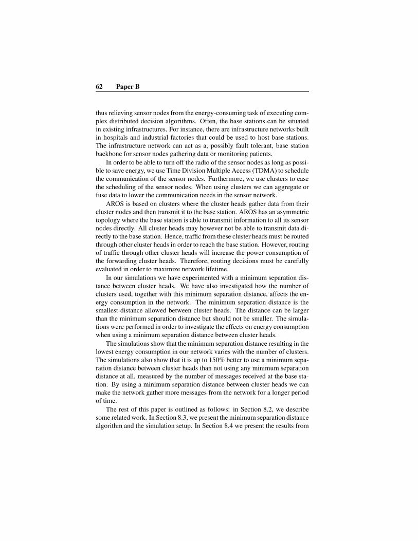
62 Paper B

thus relieving sensor nodes from the energy-consuming task of executing com-plex distributed decision algorithms. Often, the base stations can be situatedin existing infrastructures. For instance, there are infrastructure networks builtin hospitals and industrial factories that could be used to host base stations.The infrastructure network can act as a, possibly fault tolerant, base stationbackbone for sensor nodes gathering data or monitoring patients.

In order to be able to turn off the radio of the sensor nodes as long as possi-ble to save energy, we use Time Division Multiple Access (TDMA) to schedulethe communication of the sensor nodes. Furthermore, we use clusters to easethe scheduling of the sensor nodes. When using clusters we can aggregate orfuse data to lower the communication needs in the sensor network.

AROS is based on clusters where the cluster heads gather data from theircluster nodes and then transmit it to the base station. AROS has an asymmetrictopology where the base station is able to transmit information to all its sensornodes directly. All cluster heads may however not be able to transmit data di-rectly to the base station. Hence, traffic from these cluster heads must be routedthrough other cluster heads in order to reach the base station. However, routingof traffic through other cluster heads will increase the power consumption ofthe forwarding cluster heads. Therefore, routing decisions must be carefullyevaluated in order to maximize network lifetime.

In our simulations we have experimented with a minimum separation dis-tance between cluster heads. We have also investigated how the number ofclusters used, together with this minimum separation distance, affects the en-ergy consumption in the network. The minimum separation distance is thesmallest distance allowed between cluster heads. The distance can be largerthan the minimum separation distance but should not be smaller. The simula-tions were performed in order to investigate the effects on energy consumptionwhen using a minimum separation distance between cluster heads.

The simulations show that the minimum separation distance resulting in thelowest energy consumption in our network varies with the number of clusters.The simulations also show that it is up to 150% better to use a minimum sepa-ration distance between cluster heads than not using any minimum separationdistance at all, measured by the number of messages received at the base sta-tion. By using a minimum separation distance between cluster heads we canmake the network gather more messages from the network for a longer periodof time.

The rest of this paper is outlined as follows: in Section 8.2, we describesome related work. In Section 8.3, we present the minimum separation distancealgorithm and the simulation setup. In Section 8.4 we present the results from

8.2 Related Work 63

our simulations, and finally, in Section 8.5 we present our conclusions.

8.2 Related Work

LEACH (Low-Energy Adaptive Clustering Hierarchy) [3] is a TDMA clusterbased approach where a node elects itself to become cluster head by someprobability and broadcasts an advertisement message to all the other nodes inthe network. A non cluster head node selects a cluster head to join based onthe received signal strength. Being cluster head is more energy consuming thanbeing a non cluster head node, since the cluster head needs to receive data fromall cluster members in its cluster and then send the data to the base station. Allnodes in the network have the potential to be cluster head during some periodsof time. The TDMA scheme starts every round with a set-up phase to organizethe clusters. After the set-up phase, the system is in a steady-state phase for acertain amount of time. The steady-state phase consists of several cycles whereall nodes have their transmission slots periodically. The nodes send their datato the cluster head that aggregates the data and sends it to its base station at theend of each cycle. After a certain amount of time, the TDMA round ends andthe network re-enters the set-up phase.

LEACH-C (LEACH-Centralized) [6] is a variant of LEACH that uses acentralized cluster formation algorithm to form clusters. The protocol usesthe same steady-state protocol as LEACH. During the set-up phase, the basestation receives information from each node about their current location andenergy level. After that, the base station runs the centralized cluster formationalgorithm to determine cluster heads and clusters for that round. LEACH-Cuses simulated annealing [7] to search for near-optimal clusters. LEACH-Cchooses cluster heads randomly but the base station makes sure that only nodeswith “enough” energy are participating in the cluster head selection. Once theclusters are created, the base station broadcasts the information to all the nodesin the network. Each of the nodes, except the cluster head, determines its localTDMA slot, used for data transmission, before it goes to sleep until it is timeto transmit data to its cluster head, i.e., until the arrival of the next slot.

A further development is LEACH-F (LEACH with Fixed clusters) [6].LEACH-F is based on clusters that are formed once - and then fixed. Then,the cluster head position rotates among the nodes within the cluster. The ad-vantage with this is that, once the clusters are formed, there is no set-up over-head at the beginning of each round. To decide clusters, LEACH-F uses thesame centralized cluster formation algorithm as LEACH-C. The fixed clusters

64 Paper B

in LEACH-F do not allow new nodes to be added to the system and do notadjust their behavior based on nodes dying.

BCDCP (Base-station Controlled Dynamic Clustering Protocol) [8] is acentralized routing protocol with a high-energy base station that makes all thehigh energy-consuming activities e.g. selecting cluster heads and routing paths,performing randomized rotation of cluster heads. The idea in BCDCP is toorganize balanced clusters with uniform placement of cluster heads where eachcluster head serves an approximately equal number of member nodes.

During each setup phase the base station receives information on the cur-rent energy status from all the nodes in the network. BCDCP uses an iterativesplitting algorithm to form clusters. The first step is to choose two nodes,among the eligible nodes, that have the maximum separation distance. Steptwo is to group the remaining nodes to one of the cluster heads, whichever isclosest. Step tree is to balance the clusters so that each cluster has approxi-mately the same number of nodes. Step four is to start from step one and splitthe sub-clusters in to smaller parts. The iteration of the four steps continuesuntil the desired number of cluster heads is attained.

8.3 Our Approach

In order to be able to see the effects on energy consumption when using a min-imum separation distance between cluster heads, we have developed a simplealgorithm to find and select cluster heads.

8.3.1 Cluster head selection algorithm

In our cluster formation algorithm, we use the same simulated annealing asLEACH-C to minimize the energy consumption for cluster nodes when trans-mitting data to the cluster head. As LEACH-C, we randomly choose a nodeamong the eligible nodes to become cluster head but we also make sure thatthe nodes are separated with at least the minimum separation distance (if pos-sible) from the other cluster head nodes.

In the cluster head selection part, see Figure 8.1, cluster heads are randomlychosen from a list of eligible nodes. To determine which nodes are eligible, theaverage energy of the remaining nodes in the network is calculated. In orderto spread the load evenly, only nodes with energy levels above average areeligible.

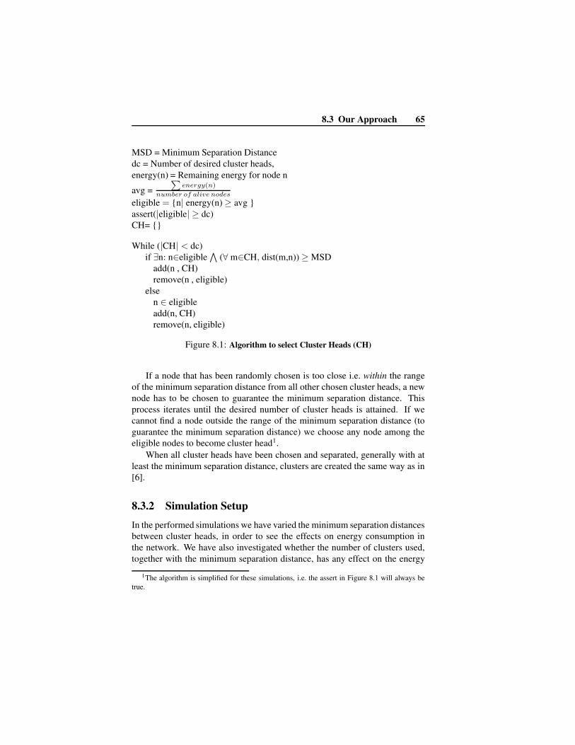
8.3 Our Approach 65

MSD = Minimum Separation Distancedc = Number of desired cluster heads,energy(n) = Remaining energy for node n

avg =∑

energy(n)

number of alive nodes

eligible = {n| energy(n) ≥ avg }assert(|eligible| ≥ dc)CH= {}

While (|CH| < dc)if ∃n: n∈eligible

∧

(∀ m∈CH, dist(m,n)) ≥ MSDadd(n , CH)remove(n , eligible)

elsen ∈ eligibleadd(n, CH)remove(n, eligible)

Figure 8.1: Algorithm to select Cluster Heads (CH)

If a node that has been randomly chosen is too close i.e. within the rangeof the minimum separation distance from all other chosen cluster heads, a newnode has to be chosen to guarantee the minimum separation distance. Thisprocess iterates until the desired number of cluster heads is attained. If wecannot find a node outside the range of the minimum separation distance (toguarantee the minimum separation distance) we choose any node among theeligible nodes to become cluster head1.

When all cluster heads have been chosen and separated, generally with atleast the minimum separation distance, clusters are created the same way as in[6].

8.3.2 Simulation Setup

In the performed simulations we have varied the minimum separation distancesbetween cluster heads, in order to see the effects on energy consumption inthe network. We have also investigated whether the number of clusters used,together with the minimum separation distance, has any effect on the energy

1The algorithm is simplified for these simulations, i.e. the assert in Figure 8.1 will always betrue.

66 Paper B

consumption. The minimum separation distance varied between 50 and 140meters, and the number of clusters varied between 2 and 15 clusters.

All simulations presented in this paper were performed within one networksetup. That is, we have used the same number of nodes and the same positionof these nodes in all experiments presented in the paper.

The simulations where performed in the network simulator NS 2 [9], us-ing a network size of 400x400 meters where 100 sensor nodes were randomlydistributed in the network. In the simulations we assume that the sensor nodesare static. We placed the base station 75 meters outside the monitored area,at location x = 200, y = 475. All sensor nodes start with a fixed amount ofenergy and the simulation continues until all the sensor nodes in the networkhave consumed all of their energy. Since AROS is an extension of LEACH,we have used the same simulation setup and radio model for our simulations asin LEACH [6], and all other parameters such as radio speed, processing delayand radio propagation speed were the same as in [6, 5].

In [6], Heinzelman has calculated how often the cluster heads should bechanged, i.e. the round-time. The calculation was made for a 100x100 metersnetwork. Due to the larger energy consumption of sending longer distances ina 400x400 meters network, we need to change cluster heads more often thanevery 20:th second, which is the round-time for the 100x100 meters network[6]. In our simulations we change cluster heads every 10:th second. Thisis a tradeoff between rescheduling cost, efficiency and energy consumptionbalance. When the network reschedules new cluster heads are chosen and newclusters are formed.

8.4 Results

In Figure 8.2, we see how the minimum separation distance affects the energyconsumption, i.e., the number of messages received at the base station duringthe lifetime of the network. We also see how the number of clusters usedaffects the energy consumption in the network. In the same figure we see thatwhen using 2 clusters, the number of messages received at the base station islow in all our simulations. Further, we see that when using 4 clusters and aminimum separation distance of 130 meters between cluster heads, the basestation receives the most messages. It is not always the case that 4 cluster yieldthe most messages to the base station. For some minimum separation distances3 cluster heads yields the most messages. Below, we have therefore looked atthe simulation results in more detail when using 3 and 4 clusters, respectively.

8.4 Results 67

0

10000

20000

30000

40000

50000

60000

2 3 4 5 6 7 8 9

Number of clusters

Num

ber

of m

essa

ges

rece

ived

at

the

base

sta

tion 0

50

70

90

130

140

MSD (m)

Figure 8.2: Messages received

In Figure 8.2, we see that using a minimum separation distance betweencluster heads is better than not to use any to control the placement of the clusterheads. By using a minimum separation distance between cluster heads we canmake the network gather more messages from the network for a longer periodof time. The figure also shows that a minimum separation distance of 130meters delivers the most messages to the base station for almost all number ofclusters.

8.4.1 Using 3 Clusters

In Figure 8.3, we present simulation results when using 3 clusters. In order tobe able to see the curves more distinctively in the figure we have chosen to onlyshow a subset of the curves2. In Figure 8.3, we see that when not using a min-imum separation distance between cluster heads, the base station receives ap-proximately 41000 messages. However, when using 3 clusters and 130 metersas the minimum separation distance, the base station receives approximately51000 messages, which is an enhancement of 24%, or 10000 messages.

2All curves not represented in the figure are located in between the curves MSD: 0 meters andMSD: 130 meters.

68 Paper B

0

20

40

60

80

100

0 5000 10000 15000 20000 25000 30000 35000 40000 45000 50000 55000

Nod

es a

live

Number of messages to the Base Station

Nodes alive vs received messages at the Base Station (Roundtime: 10 Networksize: 400x400 with 3 clusters)

MSD:0 metersMSD:70 meters

MSD:100 metersMSD:120 metersMSD:130 meters

Figure 8.3: Using 3 clusters

If we look at 80% tolerance limit3, illustrated with the upper horizontal linein Figure 8.3, we see that when not using a minimum separation distance thecurve drops below the tolerance limit already at 26000 messages. When us-ing 130 meters as the minimum separation distance the curve drops below thetolerance limit at 37000 messages, while when using 120 meters as the min-imum separation distance the curve drops below the tolerance limit at 39000messages.

Depending of the tolerance limit, different minimum separation distancesyield the longest network lifetime, e.g., the crossover point between using 120and 130 meters as the minimum separation distances is slightly above 65%sensor nodes alive, meaning that for tolerance limits above 65%, using a 120meters minimum separation distance yields the longest network lifetime (interms of messages received at the base station). The 65% tolerance limit isillustrated with the lower horizontal line in Figure 8.3.

3Most sensor networks have a lower limit on the number of nodes that must be alive in orderfor the network to still be functional, we call this limit the tolerance limit.

8.4 Results 69

In general, the spread between the minimum separation distance curves issmall in the figure and they all have a rather gradual slope (see also discussionon slope below).

8.4.2 Using 4 Clusters

0

20

40

60

80

100

0 5000 10000 15000 20000 25000 30000 35000 40000 45000 50000 55000

Nod

es a

live


Nodes alive vs received messages at the Base Station (Roundtime: 10 Networksize: 400x400 with 4 clusters)

MSD:0 metersMSD:50 metersMSD:60 metersMSD:70 metersMSD:80 metersMSD:90 meters

MSD:100 metersMSD:110 metersMSD:120 metersMSD:130 metersMSD:140 meters

Figure 8.4: Using 4 clusters

In Figure 8.4, we present simulation results when using 4 clusters. We showthat when using 4 clusters and a minimum separation distance of 130 metersbetween cluster heads, the base station receives almost 55000 messages, com-pared to the simulation with 4 clusters and no minimum separation distancewhere the base station only receives approximately 30000 messages. The min-imum separation distance of 130 meters between cluster heads thus gives anenhancement of 80%, or 25000 messages.

If we look at the 80% tolerance limit, we see that the 130 meters minimumseparation distance curve crosses the limit at about 50000 messages, while the0 meters minimum separation distance curve crosses the limit already at about

70 Paper B

20000 messages. Using 130 meters as the minimum separation distance thusgives an enhancement of 150%, or 30000 messages, compared to when notusing any minimum separation distance.

When comparing the results from using 3 clusters and 4 clusters, we seethat the number of messages received is larger for 4 clusters than for 3 clustersfor the best minimum separation distances. We can also see in the figures thatthe spread between different minimum separation distances is much larger for4 clusters than for 3 clusters, meaning that the choice of minimum separationdistance becomes much more important. It can also be noted that most curveshave a steeper slope when using 4 clusters than when using 3 clusters. Thismeans that using 4 clusters can be more advantageous for high tolerance lim-its. In our figures, when using 130 meters as the minimum separation distance,the total number of messages received is 51000 and 55000 for 3 and 4 clus-ters, respectively, a relatively small difference, less than 10%. However, whencomparing the same curves at the 80% tolerance limit, the number of mes-sages received is 37000 and 50000, respectively. Here, the relative differenceis around 30%. The conclusion from this example is that the slope of the curvematters, this will be further discussed below.

8.4.3 Minimum separation distance or not?Figure 8.6 show results from simulations with a minimum separation distanceof 130 meters and the number of clusters varied between 2 and 9. As mentionedabove, when using 4 clusters and a minimum separation distance of 130 metersbetween cluster heads, the base station receives the most messages. Whenusing the tolerance limit of 80%, the base station receives approximately 50000messages.

The bad performance when using 2 clusters can clearly be seen in Fig-ure 8.6, approximately 8000 messages are received when the 80% tolerancelimit is reached. The reason for this is that when using only 2 clusters, thecommunication distances between nodes become so long that the radio energyconsumption (which is super-linear with communication distance) increasesvery much. It can also be seen in the figure that the slope when using 3 clustersis very gradual, as was observed earlier.

Figure 8.5 shows results from simulations without minimum separation dis-tance, i.e., 0 meters as the minimum separation distance. We can see that whenusing the 80% tolerance limit and optimizing for maximum number of mes-sages received at the base station, the best configuration of the sensor networkis to use 6 clusters. The base station then receives approximately 33000 mes-

8.4 Results 71

0

20

40

60

80

100

0 5000 10000 15000 20000 25000 30000 35000 40000 45000 50000 55000

Nod

es a

live


Nodes alive vs received messages at the Base Station (Roundtime: 10 Networksize: 400x400 Minimum distance: 0)

2 clusters3 clusters4 clusters5 clusters6 clusters7 clusters8 clusters9 clusters

Figure 8.5: No Minimum Separation Distance

sages. When using 6 clusters and a minimum separation distance of 130 metersbetween cluster heads, depicted in figure 8.6, the base station receive approxi-mately 40000 messages when using the 80% tolerance limit. Using 130 metersinstead of not using a minimum separation distance thus yields an enhancementof 7000 messages.

Comparing Figure 8.5 and Figure 8.6 we see that regardless of how manyclusters we choose to use in the network, using a minimum separation dis-tance of 130 meters between cluster heads instead of not using any minimumseparation distance will make the network stay alive longer and deliver moremessages to the base station.

8.4.4 Efficient utilization

Efficient utilization of the energy resources of the sensor nodes will increasethe lifetime of the sensor network. In the ideal network, all sensor nodes wouldlive exactly the same period of time.

72 Paper B

0

20

40

60

80

100

0 5000 10000 15000 20000 25000 30000 35000 40000 45000 50000 55000

Nod

es a

live


Nodes alive vs received messages at the Base Station (Roundtime: 10 Networksize: 400x400 Minimum distance: 130)

2 clusters3 clusters4 clusters5 clusters6 clusters7 clusters8 clusters9 clusters

Figure 8.6: Minimum Separation Distance 130 meters

In Figure 8.6, we see that a more efficient utilization of the sensor nodes’power makes the sensor network stay alive a longer period of time. In the figurewe can also see that as soon as the sensor nodes in the network start to demise,the whole network demises shortly after, for all number of clusters above 3.

To be able to say that the utilization of the sensor nodes’ energy has beenefficient, we want the "knee" of the curve to be as sharp as possible, see Fig-ure 8.6. The sharper the knee is, the better the energy consumption is distrib-uted among the sensor nodes.

We want the knee to drop as late as possible and when it finally drops thegradient should be as steep as possible. This indicates that the sensor nodeshave been utilized efficiently, hence the network lives longer. This steep gra-dient also indicates that the whole network area is monitored almost until thewhole network demises.

In Figure 8.5, we see a sharp knee and a steep gradient only when using6 clusters. This indicates that most of the sensor nodes have been utilizedefficiently when using 6 clusters. Looking for sharp knees and steep gradients

8.5 Conclusions 73

in Figure 8.6, we can see that almost every choice of number of clusters have asteep gradient, except for 2 and 3 clusters, which have a more gradual slope.

When looking at Figure 8.6, we can see that when the number of clustersincreases the sharper the knee becomes. Unfortunately this is a tradeoff be-tween sharp knees and the total number of messages received. The figure showthat despite of the fact that 8 and 9 clusters have the sharpest knees, using 4clusters still delivers more messages to the base station at all times. When us-ing 8 or 9 clusters the base station receives totally 31000 and 26000 messagesrespectively, while when using 4 clusters all nodes are still alive continuingto gather information, when the base station has received the same amountof messages. This means that even though 8 or 9 clusters have the sharpestknees, using 4 clusters is still a better choice, when comparing the number ofmessages received at the base station.

8.5 Conclusions

In this paper we have presented simulation results from our experiments witha minimum separation distances between cluster heads. We have performedthese simulations in order to be able to determine how much we can lower theenergy consumption in the sensor network by separating the cluster heads, i.e.,by distributing the cluster heads through the whole network.

We have presented a simple energy-efficient cluster formation algorithmfor the wireless multihop sensor network AROS.

We have shown that using a minimum separation distance between clusterheads improves energy efficiency, measured by the number of messages re-ceived at the base station. We have also shown that it is better, up to 150% inour simulations, to use a minimum separation distance between cluster headsthan not to use any minimum separation distance. By using a minimum sepa-ration distance between cluster heads we make the network live longer, gather-ing data from the whole network area. We have also shown that the number ofclusters used together with the minimum separation distance affects the energyconsumption. Using 4 clusters and a minimum separation distance of 130 me-ters between cluster heads is the best configuration for our simulated network.

Our simulations have also shown that, depending on the number of deadnodes that can be tolerated, different minimum separation distances as well asdifferent number of clusters affects the number of messages received beforethe given tolerance limit is reached. Looking at the slope of the curve can givea good feeling of how suitable a certain configuration is; the steeper slope the

74 Paper B

better.Future work includes more thorough analysis in more scenarios with vary-

ing numbers of sensor nodes and network sizes, as well as evaluating alterna-tive algorithms for cluster head selection. A comparison between the minimumseparation distance algorithm and the BCDCP algorithm is also to be consid-ered in the future.

Bibliography


[2] M. Gerla, T.J. Kwon, and G. Pei. On Demand Routing in Large Ad HocWireless Networks with Passive Clustering. Procedings of IEEE WCNC2000, Sep 2000.

[3] W. Heinzelman, A. Chandrakasan, and H. Balakrishnan. Energy-EfficientCommunication Protocol for Wireless Microsensor Networks. Maui,Hawaii, Jan 2000. In Proceedings of the 33rd International Conference onSystem Sciences (HICSS ’00).

[4] G. Pei and C. Chien. Low Power TDMA in Large Wireless Sensor Net-works. Military Communications Conference, 1:347–351, 2001.

[5] J. Neander, E. Hansen, M. Nolin, and M. Björkman. Asymmetric MultihopCommunication in Large Sensor Networks. International Symposium onWireless Pervasive Computing 2006, ISWPC, Jan 2006.




76 Bibliography

[9] NS 2, Network Simulator. World Wide Web, http://www.isi.edu/nsnam/ns/ns-build.html, 2004.

Chapter 9

Paper C:A Study of MaximumLifetime Routing in SparseSensor Networks

Ewa Hansen, Mikael Nolin and Mats BjörkmanTo appear in proceedings of the International Workshop on Wireless Ad Hocand Mesh Networks 2008, WAMN, Barcelona, Spain, March 2008.

77

Abstract

A major issue in wireless sensor networks is to prolong network lifetime byefficient energy management. In this paper we present an initial study of max-imum lifetime routing in sparse sensor networks. We have studied simulationsof how different heuristic routing algorithms influence the energy consump-tion of individual sensor nodes, and thus the functional lifetime of a sparsesensor network. The functional lifetime of the sensor network can be eitheruntil the first node has run out of energy or until a certain threshold of nodeshas demised. We have also compared the maximum lifetime of the heuris-tic algorithms to the maximum lifetime of an optimal routing solution. Oursimulations with non-aggregated data indicates that using one of the presentedheuristic routing algorithms are not enough to find a near optimal routing. Ourstudy is made in the AROS framework.

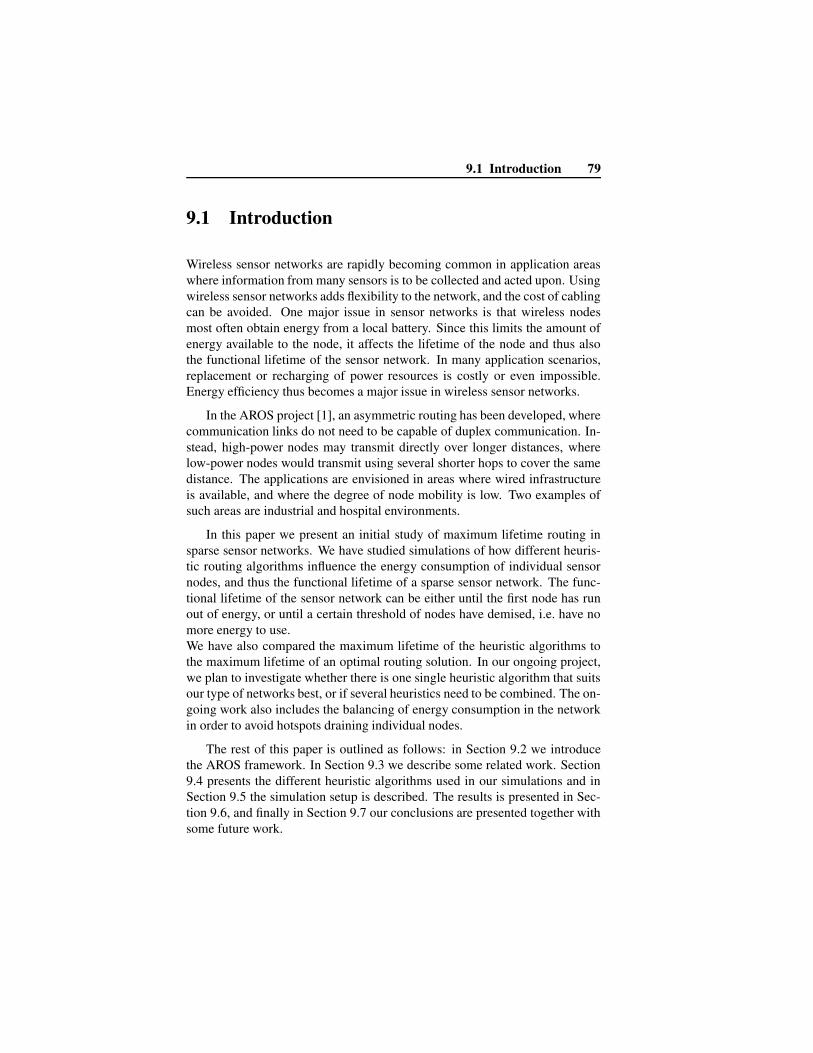
9.1 Introduction 79

9.1 Introduction

Wireless sensor networks are rapidly becoming common in application areaswhere information from many sensors is to be collected and acted upon. Usingwireless sensor networks adds flexibility to the network, and the cost of cablingcan be avoided. One major issue in sensor networks is that wireless nodesmost often obtain energy from a local battery. Since this limits the amount ofenergy available to the node, it affects the lifetime of the node and thus alsothe functional lifetime of the sensor network. In many application scenarios,replacement or recharging of power resources is costly or even impossible.Energy efficiency thus becomes a major issue in wireless sensor networks.

In the AROS project [1], an asymmetric routing has been developed, wherecommunication links do not need to be capable of duplex communication. In-stead, high-power nodes may transmit directly over longer distances, wherelow-power nodes would transmit using several shorter hops to cover the samedistance. The applications are envisioned in areas where wired infrastructureis available, and where the degree of node mobility is low. Two examples ofsuch areas are industrial and hospital environments.

In this paper we present an initial study of maximum lifetime routing insparse sensor networks. We have studied simulations of how different heuris-tic routing algorithms influence the energy consumption of individual sensornodes, and thus the functional lifetime of a sparse sensor network. The func-tional lifetime of the sensor network can be either until the first node has runout of energy, or until a certain threshold of nodes have demised, i.e. have nomore energy to use.We have also compared the maximum lifetime of the heuristic algorithms tothe maximum lifetime of an optimal routing solution. In our ongoing project,we plan to investigate whether there is one single heuristic algorithm that suitsour type of networks best, or if several heuristics need to be combined. The on-going work also includes the balancing of energy consumption in the networkin order to avoid hotspots draining individual nodes.

The rest of this paper is outlined as follows: in Section 9.2 we introducethe AROS framework. In Section 9.3 we describe some related work. Section9.4 presents the different heuristic algorithms used in our simulations and inSection 9.5 the simulation setup is described. The results is presented in Sec-tion 9.6, and finally in Section 9.7 our conclusions are presented together withsome future work.

80 Paper C

9.2 The AROS architecture

The studies presented in this paper are made in the AROS framework [1], andwe have therefore focused on sensor networks with infrastructure support. One(or more) of the network nodes is thus connected to the outside world, and to apower source such that power consumption is not an issue for that node. Sucha node we call a Base Station (BS). The Base Station acts as a receiver (sink)of all sensor information produced by the network sensor nodes.

The AROS architecture [1] is based on cluster groups using base stationswith "unlimited" energy and "enough" bandwidth in the backbone network.AROS uses a centralized approach to TDMA-based scheduling where resource-adequate Base Stations have global knowledge of the network and perform allcalculations necessary to evaluate routes and schedules, thus relieving sensornodes from the energy-consuming task of executing complex distributed de-cision algorithms. The sensor nodes periodically receive updated routing andscheduling information from the Base Station.

AROS divides the time in the network into rounds. One round is the timeduring which all sensor nodes (that wish to send data) send their data to theBase Station. After each round, routes and schedules are recalculated by theBase Station and distributed to the sensor nodes. This is done in order to mini-mize the risk of one sensor node forwarding too much data and therefore run-ning out of power much earlier than the other sensor nodes in the network.

The communication between the Base Station and the sensor nodes is asym-metric, i.e. the Base Station can communicate directly with all sensor nodes,but the sensor nodes might have to communicate with the Base Station throughother nodes, i.e. multihop.

9.3 Related Work

A lot of work has been done in the areas of energy efficient routing and poweraware routing, e.g. [2, 3, 4, 5, 6] to name a few.

Singh et al. [7] presents the PAMAS protocol which is a MAC layer pro-tocol that turns off the radio when the node is not transmitting or cannot re-ceive packets. This protocol saves 40-70% of battery power according to [7].The paper also includes several power aware metrics that are used to constructenergy-efficient routes e.g. Minimize Energy consumed/packet and MaximizeTime to Network Partition.

Li et al. [8] presents the max-min zPmin algorithm, which combines the

9.4 Heuristic algorithms 81

benefit of selecting path with both the minimum power consumption and thepath that maximizes the minimal residual power in the nodes of the network.An important factor in the max-min zPmin algorithm is the parameter z thattries to find a balance between the maximum minimum residual power pathand the minimal power consumption path, but it seems that it is not so easy tofind the optimal value of z. According to [8], the algorithm requires knowledgeabout each node in the network which can be a problem when implementing thealgorithm in large networks. To solve this problem they propose a zone-basedrouting that relies on max-min zPmin but is scalable. In zone-based routing thenetwork is divided into smaller zones, and each zone has only control over howto route the messages within its own zone. A global path across zones is alsocomputed.

Chang et al. [2] presents a flow augmentation algorithm (FA) which is ashortest cost path routing where the link cost is a combination of transmissionand reception energy consumption and the residual energy level at the two endnodes. The objective in [2] is to find the best link cost function which leadsto the maximization of the system lifetime. When there is plenty of residualenergy in the nodes, the energy cost term is emphasized, but when the node hasless residual energy, the residual energy term has greater impact,i.e. is givenmore weight in the cost function.

Shah et al. proposes in [9] a scheme called energy aware routing thatuses sub-optimal communication paths occasionally. The basic idea behind thescheme is to increase the survivability of the network by sometimes commu-nicating through a sub-optimal path. They use a set of good paths and chooseone of them, based on some probabilistic function. This means that instead ofusing one single communication path, different communication paths will bechosen at different times, thus any single communication path will not sufferfrom energy exhaustion.

9.4 Heuristic algorithms

As mentioned above, we want to maximize the functional lifetime of our net-work. Depending on the application and the amount of redundancy in thenetwork, the functional lifetime can range from the time when the first nodedemises (in the case of no redundancy) to the time when all nodes have demised(in the case of full redundancy).

Our envisioned applications (industrial, hospital, domestic) are not likely toprovide full redundancy. That means, the lifetime of individual nodes become

82 Paper C

more important. For a network with no redundancy, the optimal algorithmshould keep all nodes alive as long as possible, i.e. until all nodes run out ofenergy at the same time. For a network with some degree of redundancy, somenodes can be allowed to run out of energy early, if that prolongs the lifetime ofthe rest of the nodes.

An optimal routing strategy should be able to construct a new routingscheme for every round in the network. Since our envisioned applicationsare not fully static (albeit slow to change), the new routing schemes must beconstructed within limited time frames. Hence, it is not possible to make anexhaustive off-line scheduling of the network for its entire lifetime. Rather, thetime available to construct the new schedule is likely to be in the order of a fewseconds (or maybe even less). This implies that we must use efficient heuristicsin order to meet the timing demands of the applications.

In our first approach to find such heuristics, we have investigated the rel-ative efficiency of a number of heuristic algorithms. We want to find out ifthere is one single heuristic that suits our type of networks best. Should thisnot be the case, we want, in future studies, find under what circumstances thedifferent algorithms are most efficient. If we can find good heuristics for whento change algorithm, we could in this case be more efficient than always usingone single algorithm.

9.4.1 The algorithms studied

In order to find the most power efficient routes in our network, we have studieda number of simple heuristic algorithms that can be used to approximate theoptimal routes. In this section we describe the algorithms we have studied.

During one round, all nodes send their sensed information/data once to theBase Station. The information is either sent directly to the Base Station, orthrough other nodes. When information from all nodes has been sent to theBase Station, a new routing scheme is made and a new round begins.

Minimum total energy consumption, MTEC

In the first algorithm, MTEC, we want to minimize the total energy consump-tion for the whole network, as in equation 9.1. In equation 9.1, ei is the energyconsumption for node i when sending to the Base Station and n is the numberof nodes.

9.4 Heuristic algorithms 83

Min

n∑

i=1

ei (9.1)

The rationale behind this algorithm is that a smaller total energy consump-tion in the current round means that more energy will be left to coming rounds,i.e. the network as a whole will live longer. The balance between the energyconsumption of individual nodes is however not considered in this algorithm.

Minimum squared energy consumption, MSEC

The second algorithm, MSEC, is based on the consideration that one node canbe very heavily loaded, but the total energy consumption can still be the lowest.In this algorithm, we square the energy consumption of each individual nodebefore we sum the energy consumption, as in equation 9.2.

Min

n∑

i=1

(ei)2 (9.2)

The rationale behind this algorithm is that routes where one node is heavilyloaded will get a higher sum and thus be less likely to be chosen as the bestroute. Hence, we will get more equally loaded nodes than in the first algorithm,equation 9.1, while still choosing a route with a low total energy consumption.

Minimal maximum individual energy consumption, MMIEC

In our third algorithm, MMIEC, we minimize the maximum energy consump-tion for a single node. This is shown in equation 9.3, where emax is the maxi-mum energy consumption for a single node in the chosen route.

Min(emax) (9.3)

The rationale behind this algorithm is that if we can minimize the maximumenergy consumed by one node, we can prolong the lifetime for the node thatconsumes the most energy for a given route, and thereby prolong the lifetimeof the whole network. One drawback can be that if all nodes consume almostthe same amount of energy the network may demise quickly.

84 Paper C

Minimal difference in energy consumption, MDEC

Our fourth algorithm, MDEC, makes the difference in energy consumption be-tween the most consuming and the least consuming node as small as possible.This is shown in equation 9.4, where emax is the maximum energy consump-tion for a single node and emin is the minimum energy consumption for anothersingle node.

Min(emax − emin) (9.4)

The rationale behind this algorithm is that this algorithm makes the averageenergy consumption approximately equal between the nodes. This approachcan however be less efficient if all nodes consume a lot of energy. In this casethe difference between the nodes’ energy consumption can be small but theenergy consumption for each individual node might be high. This would leadto shorter lifetime for the network.

Maximum squared remaining energy, MSRE

In the fifth algorithm, MSRE, we have studied the remaining energy of thenodes, taking the maximal sum of the squares of the remaining energy. This isshown in equation 9.5, where eleft is the remaining energy for a single node.

Max

n∑

i=1

(elefti )2 (9.5)

This algorithm tries to maximize the remaining energy of the system. Sincethe square of the remaining energies are used in the sum, the algorithm willfavor routes where one (or more) nodes have much energy left. For networkswhere the functional lifetime of the network continues until all nodes havedemised, this can be beneficial. However, since the algorithm favors energyunbalance in the network, the first node (or nodes) is likely to demise earlierthan when using algorithms that favor energy balance.

Maximal minimum individual remaining energy, MMIRE

The sixth algorithm, MMIRE, maximizes the minimum energy left for a singlenode. This is shown in equation 9.6.

The energy left after a chosen round is calculated in advance and the mostexposed node, i.e. it has the lowest energy left, is maximized, this to not exposeone single node more than needed.

9.5 Simulation setup 85

Max(eleftmin) (9.6)

The rationale behind this algorithm is that it makes the most exposed nodeduring one round hopefully less loaded during the next rounds, thus spreadingthe energy consumption more evenly over the nodes. One drawback with thisapproach is that only one node is under consideration.

9.5 Simulation setupFor the simulations presented in this paper we have implemented a routingsystem and a simulator.

We have made simulations with 100 randomly generated sensor networks.The network area was 400x400 m2 and the number of nodes randomly spreadacross the network was 5. These nodes can be considered as either ordinarysensor nodes or cluster head nodes in a cluster-based sensor network, e.g. asin the AROS project [1]. The reason for using a small amount of nodes is thatwe want to be able to compare results from our heuristic routing algorithms toresults using an optimal routing solution. To simulate the optimal routing is tooresource-consuming to be feasible to calculate for larger numbers of nodes. Tobe able to find the optimal route, we have made a complete search among allpossible routes, and the most energy efficient1 result is found.

When calculating the energy consumption of the sensor node radio trans-mitter, we have used the same equation as in [1, 10, 11]. When sending a mes-sage a distance up to 87 meters, we have used εfriss−amp = 10pJ/bit/m2, andwhen sending a distance of more than 87 meters we have used εtwo−ray−amp =0.0013pJ/bit/m4 . The radio electronics consume Eelec = 50nJ/bit. Theequation for calculating the total amount of energy consumed when sending amessage of b bits a distance of d meters is then:

ETx =

{

b ∗ Eelec + b ∗ εfriss−amp ∗ d2 : d < 87mb ∗ Eelec + b ∗ εtwo−ray−amp ∗ d4 : d ≥ 87m

(9.7)

The amount of energy used by a sensor node radio receiver when receivinga message is:

ERx = b ∗Eelec (9.8)

1Most number of rounds.

86 Paper C

Table 9.1: Non-Aggregated dataMTEC MMIEC MDEC

a σ a σ a σ

5 nodes 13,11 13,17 15,93 14,18 14,83 12,864 nodes 7,59 8,76 5,3 11,18 4,54 10,333 nodes 6,88 11,25 6,39 12,04 6,10 13,512 nodes 13,69 29,11 11,26 30,77 11,26 33,88Total 41,27 16,36 39,38 17,70 36,73 18,57

MSRE MMIRE MSECa σ a σ a σ

5 nodes 12,27 12,38 2,07 1,60 15,27 13,954 nodes 7,49 8,72 3,28 3,68 6,16 10,963 nodes 7,09 11,70 5,59 6,30 6,56 11,942 nodes 14,79 30,92 21,35 32,59 12,62 32,86Total 41,64 16,97 32,29 16,75 40,61 18,27

In our simulations, each node starts with an energy of 0,1 mJ2. All nodesconsume energy when transmitting and receiving data packets. When not trans-mitting or receiving, the nodes are in sleep mode and are assumed to use verylittle energy. In this paper this energy is assumed negligible.

We have performed simulations with both aggregation and non-aggregationof data, where aggregation means that a downstream node can aggregate two(or more) messages of size N, bound for the same destination, into one singlemessage of size N. This enables us to study if there are differences betweenaggregation and non-aggregation with respect to what algorithms perform bestin our scenarios.

9.6 ResultsIn this section, we present some results from our studies. We have made aninitial study of maximum lifetime routing in sparse sensor networks. We havestudied simulations of how different heuristic routing algorithms influence theenergy consumption in individual sensor nodes, and thus the functional lifetimeof a sparse sensor network. We have also compared the maximum lifetime of

2The reason for the small amount of initial energy is due to the execution time of the simulation.

9.6 Results 87

the heuristic algorithms to the maximum lifetime of an optimal routing solu-tion.

The results are from simulations with non-aggregated data and from simu-lations with aggregated data. We have calculated the energy consumption ETx,using equation 9.7, when sending and ERx, using equation 9.8, when receiv-ing. All nodes that receives data consumes ERx for each message it receives.When aggregating data a node uses ETx for the one (aggregated) message itsends, and when not aggregating data it uses ETx for each message it forwards.

We have also compared the results from the different algorithms with anoptimal routing solution. The optimal routing solution in this paper is simu-lated the same way as the other algorithms, but instead of running one of theheuristic algorithms, a complete search tree is computed and the most energyefficient3 result is found.

9.6.1 Results of heuristic algorithms

In tables 9.1 and 9.2, we can see results from the six algorithms described insection 9.4. The average number of rounds (a) and the standard deviation (σ)are calculated for all the algorithms. We also show all the separate numbers ofrounds, from when the first node runs out of energy until it is only one nodeleft in the network. i.e. 5 nodes = number of rounds with all nodes alive, 4nodes = number of rounds with one node demised, and so on. Total is the totalnumber of rounds until all nodes have run out of energy. We have, in this paper,concentrated on two different functional lifetimes, as mentioned in Section 9.4.The two functional lifetimes are; until the first node demises and until all nodeshave demised.

Non-aggregated data

When looking at the results from our simulations with non-aggregated data,found in table 9.1, we can see that the average number of rounds until thenetworks have demised differs a bit among the algorithms, although in mostcases not much. When choosing route using MSRE (equ. (9.5)), we can seethat this results in the most energy-efficient routing, but using MTEC (equ.(9.1)) is almost as good. When choosing MMIRE, (equ. (9.6)) we can see thatthis approach is not quite as good as the other approaches. MMIRE is not goodat all if we want to maximize network lifetime until the first node demises. We

3Most number of rounds.

88 Paper C

can see that the other algorithms run approximately 6 to 8 times more roundsbefore the first node demises.

Another point worth noting is that MDEC has the shortest total networklifetime, if not including MMIRE. This is not surprising, since, as noted inSection 9.4, MDEC will even out energy differences, but does not consider thetotal energy consumption. An indication of this property is also that the lifetimeuntil the first node demises is relatively good for MDEC, since MDEC tries tobalance energy consumption as much as possible, thus keeping all nodes alivefor a relatively long period.

MSRE is quite the opposite to MDEC. MSRE has bad results for the num-ber of rounds until the first node demises, but has the longest total lifetime ofall algorithms. This is consistent with the discussion in Section 9.4, MSREfavors one (of a few) nodes with much energy left, and this is likely to lead tothe early demise of one of the other nodes.

Aggregated data

When looking at the results from our simulations with aggregation of data,found in table 9.2, the differences among the algorithms are not big, althoughthere are some differences. In these simulations one of the algorithms is againdifferent from the others, MMIRE (equ. (9.6)). When aggregating data, theother algorithms runs approximately 10 times more rounds, compared to MMIRE,before the first node demises.

The conclusions from these comparisons are that several of the heuristicalgorithms exhibit a similar behavior, when looking at the mean values andstandard deviations of the same 100 generated networks. Also, it is clear thatthe MMIRE algorithm is not as good as the other heuristic algorithms.

9.6.2 The algorithms compared to optimal results

When simulating the optimal routing solution, we selected one of the mostenergy-consuming networks among the 100 randomly generated networks, andcompared the result with our heuristic algorithm results. The reason for choos-ing one of the most energy-consuming networks was due to the execution timeof the optimal solution. The cost of finding the optimal solution is exponentialto the number of rounds, so only networks with small numbers of rounds arefeasible to find the optimal solution for.

9.6 Results 89

Table 9.2: Aggregated dataMTEC MMIEC MDEC

a σ a σ a σ

5 nodes 37,75 35,00 37,8 35,02 37,67 35,044 nodes 20,96 28,54 20,9 28,65 19,79 29,263 nodes 19,79 38,60 19,56 38,66 15,98 33,032 nodes 29,77 68,89 29,54 68,92 28,4 71,91

Total 108,27 42,45 107,8 42,48 101,84 42,61MSRE MMIRE MSEC

a σ a σ a σ

5 nodes 37,41 34,56 3,73 3,39 37,79 35,024 nodes 21,01 29,08 4,66 4,82 20,99 28,543 nodes 19,72 38,57 8,55 10,67 19,82 38,642 nodes 29,57 69,21 26,48 44,57 29,68 68,88

Total 107,71 42,51 43,42 22,59 108,28 42,45

Non-aggregated data

When comparing the non-aggregated results from the heuristic algorithms withthe optimal solution for non-aggregated data, the differences are more signif-icant when comparing the number of rounds until all nodes have demised.None of the heuristic algorithms could match the optimal solution of a totalof 9 rounds. The two heuristic algorithms that managed best were MTEC andMSRE with 7 rounds. MMIEC and MMIRE managed 6 rounds and MDECand MSEC only managed 5 rounds before all nodes had demised.

Comparing the number of rounds until one node had demised resulted in 3rounds for the optimal solution, MMIEC, MDEC, and MSEC. MTEC managed2 rounds and MSRE and MMIRE only 1 round. Again MMIRE, as mentionedabove, is not as good as the other algorithms.

The conclusions from this comparison are first of all that for non-aggregateddata, the heuristic algorithms were far from optimal even for a network thatonly survived 9 rounds. Also, there are clear differences between the heuris-tic algorithms when examining one single network. Finally, it is clear that theMMIRE algorithm is not a good algorithm.

90 Paper C

Aggregated data

When comparing the aggregated data simulations to the optimal routing so-lution for aggregated data, the differences are very small or none. (We onlycompared the total number of rounds, and the number of rounds until one nodehad demised.) The total number of rounds for the optimal solution and for fourof the heuristic algorithms was 13 rounds. The algorithms that were differentwere MDEC and MMIRE, which had fewer rounds, 10 and 6 respectively.

When comparing the heuristic algorithms to the optimal solution until onenode had demised, there was only one algorithm, MMIRE, that showed fewerrounds, 2, than the optimal solution. All the other algorithms showed thesame number of rounds, 4, as the optimal solution. (As mentioned earlier,the MMIRE algorithm is not as good as the other algorithms.)

9.7 Conclusions and Future WorkIn this paper we have made an initial study of maximum lifetime routing insparse sensor networks. We have studied simulations of how different heuris-tic routing algorithms influence the energy consumption in individual sensornodes, and thus the functional lifetime of a sparse sensor network. We havealso compared the maximum lifetime of the heuristic algorithms to the maxi-mum lifetime of an optimal routing solution.

We have performed simulations with 100 randomly generated sensor net-works where the network area was 400x400 m2 and the number of nodes ran-domly spread across the network was 5. The simulations were made with bothaggregation and non-aggregation of data, and a comparison with an optimalrouting solution was also done.

When looking at the simulation results with aggregated data we can seethat it is not a big difference among the heuristic algorithms. The algorithmsMSEC and MTEC are the two heuristic algorithms that show the best results.The heuristic algorithm that shows the worst results is clearly MMIRE, seetable 9.2.

When comparing these heuristic algorithms to the optimal routing solution(one of the most energy consuming network setups), the differences are verysmall or none. The total number of rounds for the optimal solution and for fourof the heuristic algorithms was 13 rounds. The algorithms that were differentwere MDEC and MMIRE, which had fewer rounds, 10 and 6 respectively.

When looking at the simulation results with non-aggregated data, the dif-ferences among the heuristic algorithms were slightly bigger. If only looking

9.7 Conclusions and Future Work 91

at the total number of rounds until all nodes have demised, MSRE, MTEC,MSEC and MMIEC were the four heuristic algorithms that performed best(when comparing both the average number of rounds and the standard devi-ation). When comparing the number of rounds until one node had demised,MSEC and MDEC were slightly better than the others. Looking at MMIRE,we can see that this heuristic algorithm is not good at all if we want to maxi-mize network life time until the first node demises.

Comparing to the optimal routing solution, the differences are more sig-nificant when comparing the total number of rounds. None of the heuristicalgorithms could match the number of rounds for the optimal solution. Thetwo heuristic algorithms that managed best were MTEC and MSRE.

The conclusions of these simulations are that when aggregating data, thechoice of heuristic algorithm is not as significant as when not aggregating data.Some differences have been identified and one of them is that MMIRE is not agood heuristic algorithm.

Our simulations with non-aggregated data indicates that using one of thepresented heuristic routing algorithms are not enough to find a near optimalrouting, hence it is possible that several different heuristic algorithms need tobe combined to find a near optimal routing solution.

In the future we will continue our work to prolong network lifetime e.g. un-til the first node demises (in sparse networks) or until some threshold of nodeshave demised (in more densely populated networks). The initial studies in thispaper is the beginning of ongoing work where we plan to investigate how wecan combine these heuristic algorithms to be able to find a near optimal routingsolution. We will investigate when to change heuristic and what heuristic thatis most suitable in different situations. We will also investigate for what kindsof network setups different heuristic algorithms are most suitable, e.g. for whatkind of network setup is MMIES most suitable? In future work we will alsotry to find a near optimal routing solution by e.g. weighting each link so thatno node drains its energy faster than the other nodes, i.e. avoiding hotspots.

Bibliography

Bibliography

[1] J. Neander, E. Hansen, M. Nolin, and M. Björkman. Asymmetric Multi-hop Communication in Large Sensor Networks. International Symposiumon Wireless Pervasive Computing 2006, ISWPC, Jan 2006.

[2] J. Chang and L. Tassiulas. Maximum lifetime routing in wireless sensornetworks. IEEE/ACM Trans. Netw., 12(4):609–619, 2004.



[5] S. Ming Tseng and R. Pandey. A Hierarchical Routing Protocol for Net-works of Heterogeneous Sensors. Goteborg, August 2004. 10th Interna-tional Conference on Real-Time and Embedded Computing Systems andApplications (RTCSA).

[6] M. Younis, M. Youssef, and K. Arisha. Energy-aware management forcluster-based sensor networks. Computer Networks, 43:649–668, Dec2003.

[7] S. Singh, M. Woo, and C. S. Raghavendra. Power-Aware Routing inMobile Ad Hoc Networks. In Mobile Computing and Networking, pages181–190, 1998.

92

[8] Q. Li, J. Aslam, and D. Rus. Online power-aware routing in wireless Ad-hoc networks. In Proceedings of the 7th annual international conferenceon Mobile computing and networking, 2001.

[9] R. Shah and J. Rabaey. Energy aware routing for low energy ad hoc sen-sor networks. In Proc. IEEE Wireless Communications and NetworkingConference (WCNC), March 2002.

[10] E. Hansen, J. Neander, M. Nolin, and M. Björkman. Energy-EfficientCluster Formation for Large Sensor Networks using a Minimum Separa-tion Distance. Lipari, Italy, Jun 2006. In Proceedings of The Fifth AnnualMediterranean Ad Hoc Networking Workshop (Med-Hoc-Net 2006).


centralized routing for prolonged network lifetime in wireless

Documents