ceo reputations and dividend payouts - nidalibdcms.nida.ac.th/thesis6/2011/b175244.pdf · ceo...
TRANSCRIPT
CEO REPUTATIONS AND DIVIDEND PAYOUTS
Danai Likitratcharoen
A Dissertation Submitted in Partial
Fulfillment of the Requirements for the Degree of
Doctor of Philosophy (Finance)
School of Business Administration
National Institute of Development Administration
2011

ABSTRACT
Title of Dissertation CEO Reputations and Dividend Payouts
Author Danai Likitratcharoen
Degree Doctor of Philosophy (Finance)
Year 2012
Over the past decades, there have been numerous discussions about the
influence of dividend policy and the value of firms. In many of the literature in this
field, frameworks have been developed to show that dividend policy has implications
for firms’ value in the imperfect and inefficient capital markets. If dividend policy has
an influence on the firm’s value, then it is worth exploring the factors that have an
influence on dividend policy. Past literature has found a large number of firm-specific
variables as the determinants of dividend policy. The purpose of this research is to test
the association between CEO reputation and the dividend payments of corporations
while controlling for firm size, market-to-book ratio, leverage, R&D spending, capital
expenditures, CEO tenure, year dummies, and industry dummies. Using press
coverage (media counts) to proxy for CEO reputation, this study conducts empirical
tests and finds that firms with reputable CEOs tend to make more investment in R&D
and tend to pay lower dividends. The logistic regression shows that firms with more
reputable CEOs are less likely to payout dividends.

ACKNOWLEDGEMENTS
I would like to thank the many people who have made this thesis possible.
First of all, I am indebted to my advisors, Associate Professor Dr. Pornsit
Jiraporn and Associate Professor Dr. Tatchawan Kanitpong, for their encouragements
and guidance throughout my thesis-writing period.
I also wish to thank the rest of my thesis committee, Assistant Professor Dr.
Viput Ongsakul and Dr. Pandej Chintrakarn, for their insightful comments.
My warm and sincere gratitude goes to my best friend, Vesarach
Aumeboonsuke for helping me get through the difficult times, for all the emotional
support, and for assisting me in many different ways.
I am grateful to my teachers at NIDA for teaching me, giving me excellent
concepts in finance, and providing me with many good ideas for doing research in
finance area.
Lastly, and most importantly, I owe my loving thanks my parents for giving
birth to me at the first place and supporting me in every way throughout my life.
Danai Likitratcharoen
April 2012
TABLE OF CONTENTS
Page
ABSTRACT iii
ACKNOWLEDGEMENTS iv
TABLE OF CONTENTS v
LIST OF TABLES vi
CHAPTER 1 INTRODUCTION 1
CHAPTER 2 LITERATURE REVIEW 5
2.1 Literature Related to Dividend Policy 5
2.1.1 Signaling 5
2.1.2 Agency Models 8
2.1.3 Catering Theory 11
2.2 Literature Related to CEO’S Reputation 13
CHAPTER 3 HYPOTHESIS 15
3.1 The Irrelevance Hypothesis 15
3.2 The Investment Hypothesis 15
3.3 The Reputation Hypothesis 16
CHAPTER 4 SAMPLE AND DATA 18
CHAPTER 5 METHODOLOGY 23
5.1 Tobit Regression 24
5.2 Logistic Regression 25
CHAPTER 6 RESULTS 27
CHAPTER 7 CONCLUSION 75
BIBLIOGRAPHY 76
APPENDIX The STATA Code 84
BIOGRAPHY 86
vi
LIST OF TABLES
Tables Page
4.1 Sample Distribution 19
4.2 Descriptive Statistics of Firm Characteristics 22
4.3 Descriptive Statistics of Dividend Payout Dummy Variable 22
5.1 Definition of Each Variable in Equation 1, 2, and 3. 23
6.1 Analysis of Variance 27
6.2 Two-Sample T-Test with Unequal Variances 28
6.3 Tobit Regression of Dividend to Total Assets on CEO’s Reputation 29
6.4 Tobit Regression of Dividend to Sales on CEO’s Reputation 33
6.5 Logit Regression of Dividend Payout Dummy on CEO’s Reputation 36
6.6 Marginal Effects after Logit Regression of Dividend Payout Dummy 41
6.7 Logit Regression of Dividend Payout Dummy on CEO’s Reputation 51
(Panel Data)
6.8 Marginal Effects after Logit Regression of Dividend Payout Dummy 54
(Panel Data)
6.9 Logit Regression of Dividend Payout Dummy on CEO’s Reputation 57
(Fixed-Effect & Panel Data)
6.10 Linear Regression of Dividend to Total Assets on CEO’s Reputation 59
6.11 Linear Regression of Dividend to Sales on CEO’s Reputation 60
6.12 The Variance Inflation Factor (VIF) Check for Multicollinearity 61
6.13 Tobit Regression of Dividend to Total Assets on Log of CEO’s 62
Reputation
6.14 Tobit Regression of Dividend to Sales on Log of CEO’s Reputation 65
6.15 Logit Regression of Dividend Payout Dummy on Log of CEO’s 68
Reputation
6.16 Linear Regression of Dividend to Total Assets on Log of CEO’s 73
Reputation74
6.17 Linear Regression of Dividend to Sales on Log of CEO’s Reputation 74
CHAPTER 1
INTRODUCTION
Over the past decades, there have been numerous discussions about the
influence of dividend policy and the value of firms. Miller and Modigliani (1961), for
example, have proposed the dividend invariance hypothesis, which illustrates that the
only determinant of a firm’s value is its investment policy, and the firm’s dividend
policy has no association with the firm’s value in perfect and efficient capital markets.
They have shown by using arbitrage argument that rational investors will be
indifferent between dividends and capital gain.
On the other hand, in some of the literature in this field, frameworks have been
developed to show that dividend policy has implications for firms’ value if the perfect
and efficient capital markets assumptions are relaxed; for example, much of the
literature on payout policy focuses on the importance of taxes. The basic aim of the
tax-related literature on dividends has been to investigate whether there is a tax effect.
If dividend income is taxed at a higher rate compared to the capital gains from stock
price appreciations, then the firms that pay out high dividends should be less valuable
than firms that pay out lower dividends.
In addition, if we relax the perfect capital market assumption and assume
instead that the capital markets are imperfect in terms of information structure, then
many researchers (Bhattacharya, 1979; Miller and Rock, 1985) suggest that when
insiders have better information about the firm’s future cash flows, dividends might
convey information about the firm’s prospects or they may be used as a costly signal
to change market perceptions concerning future earnings prospects.
Furthermore, past literature on agency models has stated that a conflict of
interest might arise between the three groups that are most likely to be affected by a
firm’s dividend policy; namely, the stockholders, management, and bondholders. The
first conflict of interest that could affect dividend policy is between management and
2
stockholders. As suggested by Jensen and Meckling (1976), managers of a publicly
held firm could allocate resources to activities that benefit them but that are not in the
shareholders’ best interest. These activities can range from lavish expenses for
corporate jets to unjustifiable acquisitions and expansions. In other words, too much
cash in the firm may result in overinvestment. Easterbrook (1984) and Jensen (1986)
have suggested a partial solution to this problem—shareholders can minimize the cash
that management controls by increasing the level of payout. This agency framework
suggests that firms paying out more dividends should have higher value than firms
paying out fewer dividends.
If dividend policy has an influence on the firm’s value, then it is worth
exploring the factors that have an influence on dividend policy. Past literature has
found a large number of firm-specific variables as the determinants of dividend
policy, such as firm size, market-to-book ratio, leverage, R&D spending, capital
expenditures, CEO tenure, and year and industry dummies.
There are several arguments justifying the positive relationship between firm
size and dividend payout. For instance, according to Redding (1997), the dividend
policy of firms is determined by the preferences of the stockholders: large institutional
investors choose to invest in large corporations because it lowers their transaction
costs. Since these institutions prefer dividends, the large corporations choose to pay
dividends, while the small corporations, owned by individuals, do not. The results
from Redding’s (1997) work show that firm size well explains the decision of whether
to pay dividends, whereas existing informational explanations (such as monitoring
and signaling) explain the level of dividends. Holder, Langrehr, and Hexter (1998)
and Twite (2001) propose that larger firms enjoy a better access to the capital market
and, consequently, are less financially constrained, which allows them to pay more
dividends. Additionally, Barclay, Smith, and Watts (1995) suggest that larger firms
are usually mature firms with limited growth opportunities that are prone to paying
more dividends in order to avoid overinvestment. Accordingly, Fama and French
(2001) provide evidence that the largest US companies have a higher payout ratio, and
more recently, Denis and Osobov (2005) show that there is the positive association
between the likelihood of paying dividends and the firm size.
3
According to Myers (1977), Market-to-book ratio, R&D spending, and capital
expenditures can serve as a proxy for growth opportunity. High market-to-book ratio,
high R&D, and high capital expenditures imply that firms have high growth
opportunity. As a result, firms with high market-to-book ratio, high R&D, and high
capital expenditures should pay fewer dividends because they have to retain more
internal funds to finance growth opportunity.
A negative association between a firm’s leverage and its dividend payout is
widely supported by financial literature namely Grossman and Hart (1980), Rozeff
(1982), Jensen (1986), and Jensen, Solberg, and Zorn (1992). As debt obligations and
dividend payouts can both be used as a way to control free cash flow or to send signal
to investors, these types of payouts are substitutes. In another word, debt and
dividends are agency-cost control mechanisms as well as by mitigating asymmetries
of information between firms and potential investors. (Ross, 1977; Harris & Raviv
1991, and Bhattacharya, 1979) This search for a trade-off between costs and benefits
leads to a substitution hypothesis based on the minimization of agency conflicts.
Therefore, firms with high leverage are expected to have less dividend payout.
According to Hu and Kumar (2004), CEO tenure can be also used as a proxy
for managerial entrenchment. This entrenchment can be defined as the likelihood of a
manager to opt for concentrated power. These authors find that both the likelihood
and the level of dividend payouts are significantly and positively (negatively) related
to the factors that increase (decrease) executive entrenchment levels, even when
controlling for firm characteristics, such as firm size, leverage, book-to-market ratio,
and the proportion of tangible to total assets.
Year and industry dummies have also been used as additional control variables
in order to test whether the association between dividend payout and explanatory
variables is constant across industries and over time. Besides the explanatory
variables mentioned above, this paper adds one more explanatory variable—that is,
CEO reputation. The reason that this study includes CEO reputation is motivated by
three considerations. First, CEO reputation is one of the most important intangible
assets that a firm has (Gaines-Ross, 2003) second, it captures the dimension of
managerial human capital (Francis, Huang, Rajgopal and Zang, 2008) and last,
according to Burson-Marsteller’s survey in 1999, almost half of a firm’s reputation is
4
based upon the image of its CEO. Thus, this CEO characteristic can potentially have
an impact on corporate policies. As a result, the purpose of this research is to test the
association between CEO reputation and the dividend payments of corporations while
controlling for firm size, market-to-book ratio, leverage, R&D spending, capital
expenditures, CEO tenure, year dummies, and industry dummies.
The contributions of this paper are as follows. First, the evidence presented in
this study will reveal whether CEO reputation—a manager-specific characteristic—
will affect the firm’s dividend policy or not. Second, this study is related to the
literature in behavioral finance and will test whether CEOs that enjoy a strong
reputation will make more investment or not. The behavioral decision theory predicts
that overconfident CEOs are inclined to take more risks (Nosic and Weber, 2010; Gao
and Sudarsanam, 2005). For this reason, these overconfident CEOs tend to pay out
fewer dividends and to retain more funds for future investment opportunities because
they are confident that they will be able to get a higher rate of return from future
investments and that the investments they make will contribute to higher growth for
the firm compared to the scenario in which the firm pays out dividends. Third,
whether reputable CEOs use internal funds for fixed investments or R&D investments
will be tested in this study.
CHAPTER 2
LITERATURE REVIEW
2.1 Literature Related to Dividend Policy
2.1.1 Signaling
Because capital markets are imperfect, information asymmetry exists between
managers (insiders) and outside investors. If managers have better information about
firms’ future cash flows, it has been suggested by many researchers that dividends
might convey information about these firms’ prospects, and dividends may be used as
a costly signal to change market perceptions concerning future earnings prospects.
If it is assumed that the source of funds for the firm is equal to the use of funds
and that the firm’s investment is known, dividend announcements could convey
information about current earnings (and about future earnings if they are serially
correlated) because the firm’s earnings are equal to investment plus dividends. In this
way, dividends that are larger than expected imply higher earnings, and since the
market does not necessarily know the current level of earnings, these higher-than-
anticipated earnings will lead to a positive stock price increase. The most well-known
work that has developed this concept of signaling models is that of Bhattacharya,
1979; Miller and Rock, 1985; and John and Williams, 1985. The basic idea in all of
these models is that firms adjust dividends to signal prospects—a rise in dividends
will signal that the firm will perform better and a decrease suggests that it will
perform less well.
In Bhattacharya’s (1979) two-period model, at time zero, the managers invest
in a project; they know the expected profitability of this investment but investors do
not. The managers also commit to a dividend policy. Then at time 1, the “project
generates a payoff that is used to pay the dividends committed to at time zero.” A
crucial assumption of this model is that if the payoff is not sufficient in terms of
covering the dividends, the firm must raise external funds and this will result in
6
transaction costs for the firm. At time zero, the managers can signal that the firm’s
project is good by committing to a large dividend at time 1; and if a firm does have a
good project, it will likely be able to pay the dividend without this resorting outside
financing and therefore will not have to incur any transaction costs associated with the
action. It is not a good idea, however, for a firm that has a bad project to do this
because it will have to resort to outside financing more frequently and will then have
to suffer from higher transaction costs.
Miller and Rock (1985) have also created a two-period model, and in this
model, when firms invest in a project at time zero, their profitability will not be
observed by investors. At time 1, the project produces earnings and the firm uses
these earnings to finance its dividend payment and new investment. Investors will not
be able to observe either earnings or the new level of investment. At time 2, on the
other hand, the investments of firms again produce earnings. A critical assumption of
the model is that these earnings will be correlated through time. This thus implies that
the firm has a good reason to make shareholders believe that the earnings at time 1 are
high and in this way shareholders who sell will receive a high price. Since both
earnings and investment are unobservable, a firm that does not perform well can make
others believe that it has high earnings by cutting its investment and instead paying
out high dividends. A good firm must pay a level of dividends that is sufficiently high
so that it will be perceived as unprofitable for bad firms to reduce their investment
sufficiently to achieve the same level of dividends.
In Bhattacharya’s (1979) the dissipative cost that allows signaling to occur is
the transaction cost of having to rely on outside financing. Bhattacharya posits that
the dissipative costs arise because increasing dividend payout forces the firm into the
capital market more frequently, thus resulting in increased financing costs. In Miller
and Rock’s (1985) model, on the other hand, dissipative costs stem from the distortion
in the firm’s investment decisions. John and Williams (1985) have presented a model
in which taxes represent dissipative cost, and as a consequence, the theory adequately
addresses the criticism that the same signal can be achieved at a lower cost if the firm
instead repurchases shares. While Miller and Rock’s and Bhattacharya’s models
suggest that dividends and repurchases are good substitutes for share repurchases,
John and Williams’ model suggests that dividends and repurchases are not related; in
7
the words of Allen and Michaely (2002), “[a] firm cannot achieve its objective of
higher valuation by substituting a dollar of dividends for a dollar of capital gains.”
A number of theories with multiple signals have been developed after Miller
and Rock’s (1985) and John and Williams’ (1985) work. Ambarish, John, and
Williams (1987), for example, constructed a single-period model with dividends,
investment, and stock repurchases. Bernheim (1991) also provided a theory of
dividends, according to this theory, signaling happens because dividends are taxed
more heavily than repurchases. In his model, the amount of taxes paid is controlled by
the firm by varying the proportion of total payout in the form of dividends rather than
in the form of repurchases—a good firm can choose an optimal amount of taxes in
providing the signal.
A different approach to dividend signaling was taken by Allen, Bernardo, and
Welch (2000). As in the previous models, dividends are seen as a signal of positive
information (undervaluation). In their model, however, firms pay dividends because
they are interested in attracting a clientele that has a better grasp of the reality of the
situation. In this case, untaxed institutions, for example, pension funds and mutual
funds, will be the primary holders of dividend-paying stocks because they represent a
tax-disadvantaged payout method for other stockholders.
Another reason that institutions hold dividend-paying stocks concerns
restrictions in institutional charters, such as the “prudent man” rules that make it
difficult for many institutions to purchase stocks that pay either no dividends or low
dividends. According Allen, Bernardo, and Welsh (2000), the reason that good firms
like institutions to hold their stock is that these stockholders have a better
understanding of firm quality and possess an advantage in knowing when a firm is of
high quality. The low-quality firms do not have the incentive to copy the behavior of
other firms because they do not want their true worth to be shown. As a result, taxable
dividends are desirable because they allow the management of firms to demonstrate
the good quality of their firms.
One other interesting aspect of the Allen, Bernardo, and Welch’s model is that
it takes into consideration dividend “smoothing;” that is, firms that pay dividends are
unlikely to reduce the amount of the dividend because their clientele (institutions) will
respond negatively. For this reason dividends are kept relatively smooth.
8
Grullon, Michaely, and Swaminathan (2002) have presented an alternative
explanation of the reason why stock price increases when a firm pays more dividends.
They refer to this as the “maturity hypothesis,” in which they propose that there are
several elements contributing to the maturation of firms. For example, as firms
mature, their investment opportunities shrink and this results in a potential decline in
future profitability. The most important result of firms becoming mature, however, is
the change in its risk characteristics, and specifically in the decline of risk—a decline
in risk most likely occurs because firms’ current “assets in place” have become less
risky or because they exhibit fewer growth opportunities. In the end, a decline in
investment opportunities will generate an increase in free cash flows and this will lead
to an increase in dividends. It is for this reason that a dividend increase indicates that
a firm has matured.
According to the maturity hypothesis, dividends are increased by firms when
growth opportunities decline, thus leading to a decrease in systematic risk and
profitability of the firm. The market will then perceive this dividend increase from
two points of view: that is, that the risk has decreased, and that profits are going to
decline. If the market reaction is positive, the idea of risk will dominates news about
profitability.
2.1.2 Agency Models
Another explanation of why stock price increases when a firm pays out more
dividends is that investors will treat dividend increases positively because of agency
considerations in spite of declining profitability. If investors expect managers to
consume a firm’s wealth by overinvesting, for example, then a dividend increase
suggest that managers will have the inclination to act more responsibly. In addition to
this positive information concerning risk reduction, investors might interpret a
dividend increase in a positive light as they reduce overinvestment problems; stock
prices will then increase.
According to the literature, three groups are most likely to be affected by a
firm’s dividend policy: stockholders, management, and bondholders. The first conflict
of interest that can affect dividend policy is between management and stockholders
(the separation of ownership and control). As suggested by Jensen and Meckling
9
(1976), the stockholders own the firm whereas the managers control the firm. Ideally,
the managers should act according to the stockholders’ best interests however, in
reality the managers of a publicly-held firm could allocate resources to the activities
that benefit them but that are not in the shareholders’ best interest. These activities
can range from expensive acquisitions such as jets to items that are more
questionable. In additions, the managers may invest in many unprofitable or unrelated
projects just to expand the firm size and secure their job positions or to fulfill their
personal interests. In other words, too much cash in the firm can end in overinvestment.
Grossman and Hart (1980), Easterbrook (1984), and Jensen (1986) have
suggested a partial solution to this problem: if stockholders can minimize the cash
controlled by management, they can make it much more difficult for management to
continue to spend money in an unmonitored fashion; and the less discretionary money
that management has, the more difficult it will be for them to invest in negative NPV
projects. According to some of advanced in the literature, one way to remove
unnecessary cash from the firm is to increase the level of payout; these theories
suggest a significant departure from the original assumption by Miller and Modigliani
in the sense that payout policy and investment policy are interrelated—paying out
cash would increase the value of the firm by reducing potential overinvestment.
One drawback of these theories is that they fail to explain why firms pay out
in the form of dividends instead of share repurchases, since share repurchases are a
cheaper way to remove money from management. Another related question is the
following: why should management be monitored through payout and not through
debt? As Grossman and Hart (1980) and Jensen (1986) have argued, a mechanism that
would be more effective in achieving this goal would be to increase the level of debt:
it is more difficult for management to go back on a debt commitment than on a
dividend commitment. This argument can also be related to the choice of dividends
versus repurchases. If it is assumed that the market strongly dislikes dividend
reductions, and that management is therefore reluctant to reduce dividends, then it can
be seen that dividends represent a more effective mechanism than repurchases in
terms of imposing discipline.
The second drawback of Agency Theory is that, although it offers a good
explanation of dividend increases, as stated in the literature for example by Grossman
10
and Hart (1980), Easterbrook (1984), and Jensen (1986), this explanation does not
apply as well to dividend decreases. Firms increase dividends when they have free
cash flow, and a positive market reaction to a dividend announcement can occur
because the market realizes that management will have to be more disciplined in its
action. Further, concerning dividend cuts, one possibility is that management can cut
dividends when cash flow falls; hence there should be a positive market reaction to
the announcement of dividend cuts due to the decrease in free cash flows (because the
decrease in free cash flows will force the manager to be more disciplined). Another
possibility is for management to cut dividends when there is good investment; in this
way, the cut would also be greeted in a positive way by the market. This situation
does not happen frequently, however, because in this case good investments could be
financed by debt.
The work of Allen, Bernardo and Welch (2000) provide a framework that can
partially solve the first problem; i.e. dividends as opposed to repurchases. If some
large shareholders view the tax treatment of dividends in a positive light, for example
corporations, then it would be possible for dividends to be paid in order to attract this
type of investors. In fact, Allen, Bernardo, and Welch (2000) have extended this
analysis and have demonstrated that a favorable tax rate for institutions in relation to
individuals will encourage large shareholders to prefer dividend-paying stocks. This
view of clientele effect can then include not only corporations but also various types
of institutions that are not subject to taxation.
These low tax-bracket investors will increase the value to all shareholders
since they monitors management and thereby increase firm value. A question of
whether large shareholders are attracted to firms that pay dividends is an unresolved
empirical issue.
Apart from the first conflict of interest, which is between shareholders and
managers, the second conflict of interest that may be affected by payout policy is
between stockholders and bondholders. As Myers (1977) and Jensen and Meckling
(1976) have argued, there are some situations in which equityholders might try to
expropriate wealth from debtholders. This wealth expropriation could come in the
form of excessive and unanticipated dividend payments. Shareholders can reduce
investments and thereby increase dividends (investment-financed dividends), or they
11
can raise debt to finance the dividends (debt-financed dividends). In both cases, if
debtholders do not anticipate the shareholders’ action, then the market value of debt
will go down and the market value of equity will rise.
2.1.3 Catering Theory
The more recent finance literatures attempt to model the dividend payout by
incorporating the psychological component and proposed that an important part of the
firm’s decision to pay dividends may be due to a firm’s desire to satisfy investors’
expectations. For instance, Shefrin and Statman (1984) develop the “behavioural life
cycle” theory of dividends, which relies on psychological reasons to explain why
investors prefer dividends rather than capital gains. Feldstein and Green (1983) find
that dividend policy is affected by investors’ consumption needs. Polk and Sapienza
(2004) and Baker, Stein, and Wurgler (2003) also rely on behavioral explanations to
explain the clientele effect.
One of the most popular literatures that consider the principles of behavioral
finance in the dividend payout is a catering theory of dividends developed by Baker
and Wurgler (2004a), which proposed that firms cater to their investors’ preferences
so that they pay dividends when dividend payers trade a premium and do not pay
dividends when dividend payers trade a discount. According to Baker and Wurgler
(2004a), the difference between the catering theory and the clientele theory is that the
clientele theory does not explore dividends through the investors’ sentiments, whereas
the catering theory does. Moreover, the clientele focuses more on the firm level but
the catering theory focuses more on the global level of dividends as the result of the
demand for shares that pay dividends.
Baker and Wurgler (2004b) provide empirical evidence to support their theory.
They show that changes in the proportion of the dividend-payer firms along the time
can be explained in terms of the catering incentives. Catering incentives is a measure
of the market desire for dividend-paying stocks. They also find a connection between
the tendency to pay dividends and catering incentives. In their work, the dividends
premium is used as a proxy for the value that the market places on dividends i.e., the
premium that the investors are willing to pay for dividends-paying stocks.
12
Baker and Wurgler (2004b) measure the relative investors’ sentiment about
dividend paying firms by using the difference between the logarithm of the book-
value-weighted average market-to-book ratio for dividend payers and the book-value-
weighted average market-to-book ratio for non-payers. They find a positive
relationship between the catering incentives (the dividend premium) and the change in
firms’ propensity to pay dividends.
There have been many studies providing the empirical evidence to support this
theory. Bulan et al. (2005) presents evidence consistent with the dividend catering
theory by showing that the timing of dividend initiation is affected by the investors’
sentiment, measured by the dividend premium. The firms that have higher dividend
premium are more likely to initiate dividend than the firms with lower dividend
premium. Additionally, Denis and Osobov (2005) provide the time series evidence on
the propensity to pay dividend in several developed financial markets in civil law
countries (France, Japan, Germany) and common law countries (U.S., Canada, and
United Kingdom). Their findings show that dividend premium is a measure of relative
growth opportunity of payers and non-payers rather than a measure of investor
sentiment for dividend. Another study related to catering theory in common law and
civil law countries has been conducted by Ferris, Jayaraman, and Sabherwal (2009).
Their study tests for the international presence of dividend catering across a sample of
twenty-three countries and find evidence of catering among firms incorporated in
common law countries but not for those in civil law countries.
Furthermore, Li and Lie (2006) extend Baker and Wurgler’s catering theory
by including decreases and increases in existing dividends. Their finding is consistent
with the catering theory and also the results provide additional evidence that dividend
changes depend on the dividend premium. They find that dividend premium has
significant explanatory power of dividend initiations, dividend changes, and changes
in the propensity to pay dividends.
On the contrary, several empirical evidences show that firms do not pay
dividend as predicted by catering theory. Hoberg and Prabhala (2005) find that
catering becomes statistically and economically insignificant when control for risk.
Their result show that risk is an important determinant of dividend decisions, but
dividend policies cater to investor sentiment is an unimportant factor. Additionally,
13
Tsuji (2010) tests the catering theory with the firms in Japanese electrical appliances
industry and finds that dividend initiation decisions of these firms have no predictive
power for the relative future returns of payers over non-payers, the dividend premium
is not a determinant of the dividend initiations of the firms, and the dividend premium
has no relation with the dividend continuation decisions of the firms.
2.2 Literature Related to CEO’S Reputation
Few works in the finance and economics literature have considered the effects
of managerial characteristics on firm investment and financing decisions. Bertrand
and Schoar (2003) found that managerial style affects a firm’s corporate policy
decisions and these differences were also seen in the compensation levels of
managers. Richardson, Tuna, and Wysocki (2003) found that firms that share
common directors also share the following: governance, financial, disclosure, and
strategic policy choices. Chevalier and Ellison (1999) have conducted an investigation
on the effect of the age and schooling of the mutual fund manager on the performance
of funds. They found that younger managers and managers that had attended good
schools earned higher rates of return. Graham and Harvey (2001) in turn have
provided survey-based evidence that CFOs with an MBA degree use more
sophisticated valuation techniques compared to those that do not have an MBA
degree.
In Milbourn’s (2003) study, he focused on the CEO’s reputation and measured
it in terms of the number of press articles that cited the CEO. He found that
compensation contracts given to CEOs with a good reputation (i.e., those with more
media-counts) exhibited greater pay-for-performance sensitivity. Liu, Zhang and
Jiraporn (2011), on the other hand, investigated the relationship between the CEO’s
reputation and corporate risk-taking; and their empirical results indicated that
reputable CEOs tend to take more risks, “especially idiosyncratic and unlevered
risk[s]” (Liu, Zhang and Jiraporn, 2011). Investigations on the channels of risk-taking
activities have revealed that CEOs with strong reputations tend to seek R&D
investments but avoid higher financing risks. Finally, a study on the impact of the
CEO’s reputation on credit ratings found that firms in which the CEO enjoyed a
14
strong reputation experienced lower credit ratings. These results suggest that a
manager-specific attribute such as reputation can have a significant impact on
important corporate outcomes and can influence corporate risk-taking. These results
are still robust even after controlling for a large number of firm-specific variables,
such as firm size, market-to-book ratio, leverage, R&D spending, capital
expenditures, CEO tenure, and year and industry dummies. In terms of economic
significance, a one-standard-deviation shock in CEO’s reputation increases firm risk
by as much as 16.16%; thus the impact of a CEO’s reputation can be considered
statistically significant as well as economically meaningful. In fact, a good reputation
can have a negative outcome; according to March and Shapira (1987), Sitkin and
Pablo (1992), Kahneman and Lovallo (1993), and Liu, Zhang and Jiraporn (2011), a
strong reputation may create overconfidence, resulting in the CEO’s overestimation of
his or her problem-solving capability and, as a result, the CEO might exhibit more
aggressive risk-taking behavior.
CHAPTER 3
HYPOTHESIS
3.1 The Irrelevance Hypothesis
This hypothesis assumes that managers are homogeneous and selfless inputs
into the production process. It also suggests that different managers can be regarded
as perfect substitutes for one another. Many prior studies have subscribed this view
and have assumed that top managers do not matter. Although executives may possess
different preferences, degrees of risk aversion, or skill levels, none of them translates
into actual corporate policies. Furthermore, individual managers may be constrained
by organizational structure and external forces so much that their individual
characteristics do not influence corporate behavior (Hannan and Freeman, 1977;
DiMaggio and Powell, 1983; Liu, Zhang and Jiraporn, 2011). This hypothesis predicts
that CEO reputation has no association with the dividend payouts of firms.
3.2 The Investment Hypothesis
This perspective argues that a CEO that enjoys a strong reputation is
vulnerable to make more investment, and a highly reputable CEO tends to be
overconfident, take more risks and more investment. The association between CEO
reputation and overconfidence is mentioned in the work of Francis et al. (2004),
Malmendier and Tate (2005, 2005b), Jin and Kothari (2006) and Hribar and Yang
(2007). Francis et al. (2004) suggests that CEO reputation can be a proxy by using the
total number of media mentions. Malmendier and Tate (2005, 2005b) classify the
CEO as overconfident if he/she is more frequently described as confident and
optimistic relative to descriptors such as frugal, conservative, cautious, practical,
reliable, or steady. Further, Hribar and Yang (2007) found that the number of media
16
mentions is positively correlated with other measures of CEO confidence. This
finding is consistent with Francis et al. (2004), who used this variable as a proxy for
CEO reputation to examine the association between management reputation and a
firm’s earnings quality. The behavioral decision theory predicts that overconfident
CEOs increase the firm’s risk-taking (Kahneman and Lovallo, 1993; March and
Shapira, 1987; Sitkin and Pablo, 1992). The theory suggests three mechanisms that
link CEO overconfidence to the degree of risk-taking: first, overestimation of the
CEO’s own problem-solving capabilities (Camerer and Lovallo, 1999); second,
underestimation of a firm’s resource endowments (Shane and Stuart, 2002); and third,
underestimation of the uncertainties that the firm is facing (Kahneman and Lovallo,
1993; March and Shapira, 1987). These three mechanisms tend to allow an
overconfident CEO to interpret decision situations as less risky than they actually are,
and thus to take more risks (Chatterjee and Hambrick, 2007; Sitkin and Pablo, 1992).
Investment and financing decisions are two major corporate policy decisions
and therefore they are the main potential channels by which CEOs increase firm risk.
If reputable CEOs tend to take greater risks, then greater investment in risky projects
should be observed in firms with reputable CEOs. Investment can be financed by
internal funds and external funds; however, bondholders often place restrictions on
firm leverage ratios in debt covenants in order to protect their interests, so increasing
leverage through debt issues may not be an optimal choice for reputable CEOs.
Moreover, reputable CEOs that are overconfident tend to believe that the stock of
their companies is underpriced, so increasing external funds by issuing equity may
also not be an optimal choice for them. As a result, reputable CEOs may prefer to use
internal funds to finance the investment in risky projects. Based on these conjectures,
this hypothesis predicts a negative relationship between reputable CEOs and dividend
payouts.
3.3 The Reputation Hypothesis
This view argues that reputable CEOs exhibit a higher degree of risk
aversion. Amihud and Lev (1981), Hirshleifer and Thakor (1992), and Holmstrom
and Ricart I Costa (1986) argue that managers avoid taking risks because of career
17
concerns and possible damage to their image. Career concerns of CEOs have been
found to affect CEO behavior (Amihud and Lev, 1981; Hirshleifer and Thakor, 1992;
Holmstrom and Ricart I Costa, 1986; and Gilson, 1989, 1990). Reputable CEOs have
more to lose than less reputable ones and are expected to be more risk-averse. Gilson
(1989, 1990) documents that top managers experience a large personal cost
(reputation) when firms default. Warren Buffett once said, “it takes twenty years to
build a reputation and five minutes to destroy it.”
A strong reputation is crucial to a CEO’s career for several reasons. First,
reputable CEOs are more likely to be invited to join other boards as outside directors
(Kaplan and Reishus, 1990; Gilson, 1990; Brickley, Linck and Coles, 1999; Ferris,
Jaganathan and Pritchard, 2003). Second, CEOs with a strong reputation are more
likely to stay on as chairmen of the board. Furthermore, a strong reputation may
create not only board service, but also consulting opportunities, related professional
opportunities such as legal or securities arbitrations, status in the community,
judgeships, and other opportunities available principally to those with a strong
reputation (Brickley, Linck and Coles, 1999). Because the reputable CEOs would
have more to lose if their firms perform poorly, they tend to need less fund for making
investments and therefore payout more dividends. Based on these arguments, this
hypothesis predicts a positive relationship between reputable CEOs and dividend
payouts.
CHAPTER 4
SAMPLE AND DATA
This study uses S&P 500 companies over the period 1992-2007, as identified
from the ExecuComp database. CEO reputation is measured based on how parties
external to the firm view the CEO, as reflected in the number of articles containing
the CEO’s full name and company affiliation that appeared in major U.S. and global
business newspapers and newswires in calendar year t. In particular, following
Milbourn (2003), Francis et al. (2008), and Liu, Zhang and Jiraporn (2011), the search
for press releases was conducted in the following major U.S. and international
newspapers: the Wall Street Journal, the New York Times, the Washington Post, USA
Today, the Financial Times, the Asian Wall Street Journal, Wall Street Journal
Europe, and the International Herald Tribune. An article is included once if it contains
the CEO’s full name and company name, irrespective of how many times the name
appears in the article. The total number of article counts in a year was used as a proxy
for the CEO’s reputation in that year (Milbourn, 2003; Rajgopal et al., 2006; Liu,
Zhang and Jiraporn, 2011).
Francis et al. (2008) ensure that the number of citations is not a reflection of
CEO infamy as opposed to reputation by conducting three validation checks. First,
when the articles are randomly selected, the tone is favorable toward the CEO 95% of
the time. Second, the number of press coverage is correlated with a proxy for
reputation used by Milbourn (2003) and Rajgopal et al. (2006) who used the numbers
of CEOs appointed from outside the firm as a proxy for reputation. Third, the number
of citations is highly correlated with explicit recognition of the CEO by the “top
CEO” lists compiled by various sources. The results of these validity checks justify
the use of press coverage or total citations as a measure of the CEO reputation.
Accordingly, similar to their research, this paper also uses the press coverage as a
proxy for CEO reputation.
19
The financial data were obtained from Compustat and stock returns from
CRSP. This study excluded financial and utility firms from the sample. The final
sample had 4,036 CEO-year observations corresponding to 316 unique firms.
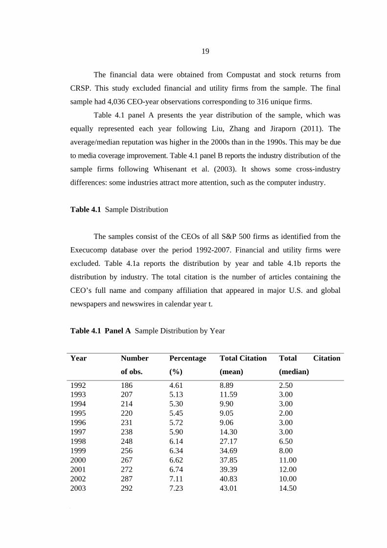
Table 4.1 panel A presents the year distribution of the sample, which was
equally represented each year following Liu, Zhang and Jiraporn (2011). The
average/median reputation was higher in the 2000s than in the 1990s. This may be due
to media coverage improvement. Table 4.1 panel B reports the industry distribution of the
sample firms following Whisenant et al. (2003). It shows some cross-industry
differences: some industries attract more attention, such as the computer industry.
Table 4.1 Sample Distribution
The samples consist of the CEOs of all S&P 500 firms as identified from the
Execucomp database over the period 1992-2007. Financial and utility firms were
excluded. Table 4.1a reports the distribution by year and table 4.1b reports the
distribution by industry. The total citation is the number of articles containing the
CEO’s full name and company affiliation that appeared in major U.S. and global
newspapers and newswires in calendar year t.
Table 4.1 Panel A Sample Distribution by Year
Year Number
of obs.
Percentage
(%)
Total Citation
(mean)
Total Citation
(median)
1992 186 4.61 8.89 2.50 1993 207 5.13 11.59 3.00 1994 214 5.30 9.90 3.00 1995 220 5.45 9.05 2.00 1996 231 5.72 9.06 3.00 1997 238 5.90 14.30 3.00 1998 248 6.14 27.17 6.50 1999 256 6.34 34.69 8.00 2000 267 6.62 37.85 11.00 2001 272 6.74 39.39 12.00 2002 287 7.11 40.83 10.00 2003 292 7.23 43.01 14.50
20
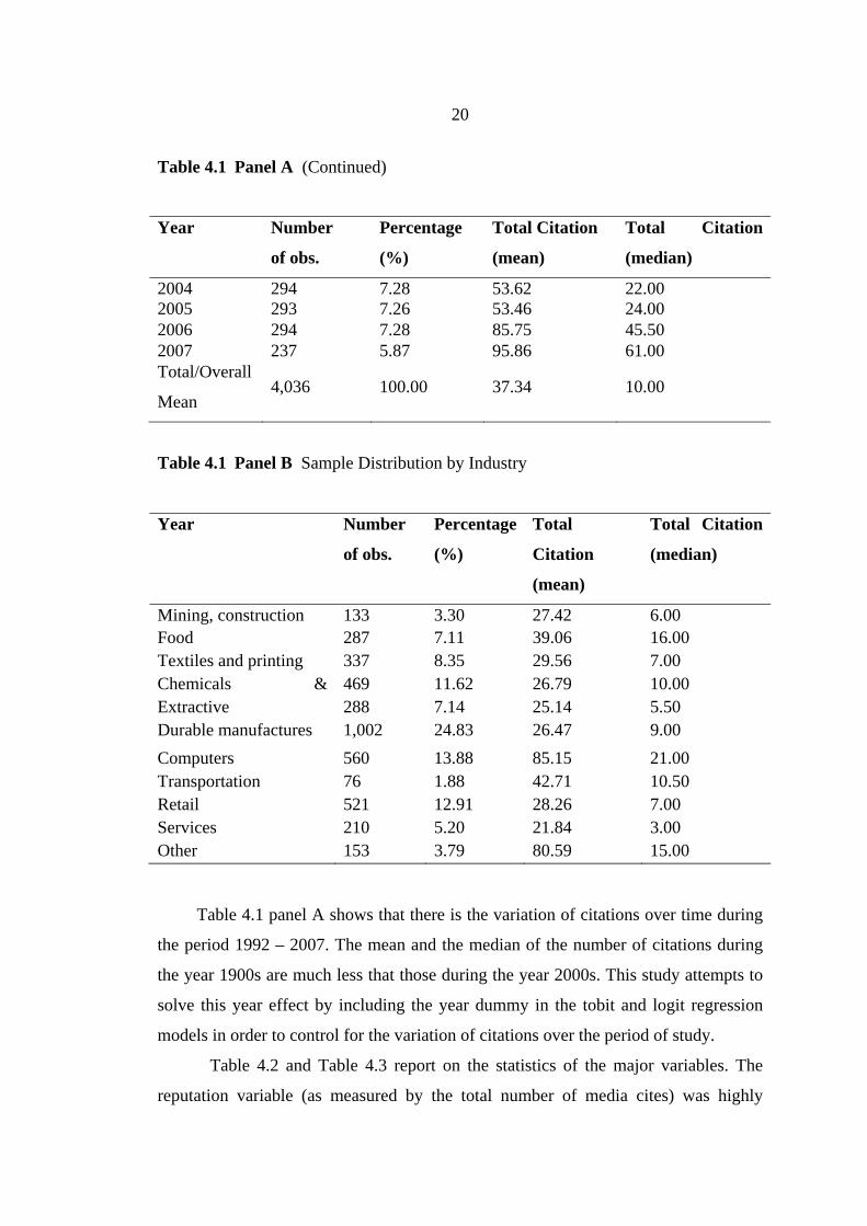
Table 4.1 Panel A (Continued)
Year Number
of obs.
Percentage
(%)
Total Citation
(mean)
Total Citation
(median)
2004 294 7.28 53.62 22.00 2005 293 7.26 53.46 24.00 2006 294 7.28 85.75 45.50 2007 237 5.87 95.86 61.00 Total/Overall
Mean 4,036 100.00 37.34 10.00
Table 4.1 Panel B Sample Distribution by Industry
Year Number
of obs.
Percentage
(%)
Total
Citation
(mean)
Total Citation
(median)
Mining, construction 133 3.30 27.42 6.00 Food 287 7.11 39.06 16.00 Textiles and printing 337 8.35 29.56 7.00 Chemicals & 469 11.62 26.79 10.00 Extractive 288 7.14 25.14 5.50 Durable manufactures 1,002 24.83 26.47 9.00 Computers 560 13.88 85.15 21.00 Transportation 76 1.88 42.71 10.50 Retail 521 12.91 28.26 7.00 Services 210 5.20 21.84 3.00 Other 153 3.79 80.59 15.00
Table 4.1 panel A shows that there is the variation of citations over time during
the period 1992 – 2007. The mean and the median of the number of citations during
the year 1900s are much less that those during the year 2000s. This study attempts to
solve this year effect by including the year dummy in the tobit and logit regression
models in order to control for the variation of citations over the period of study.
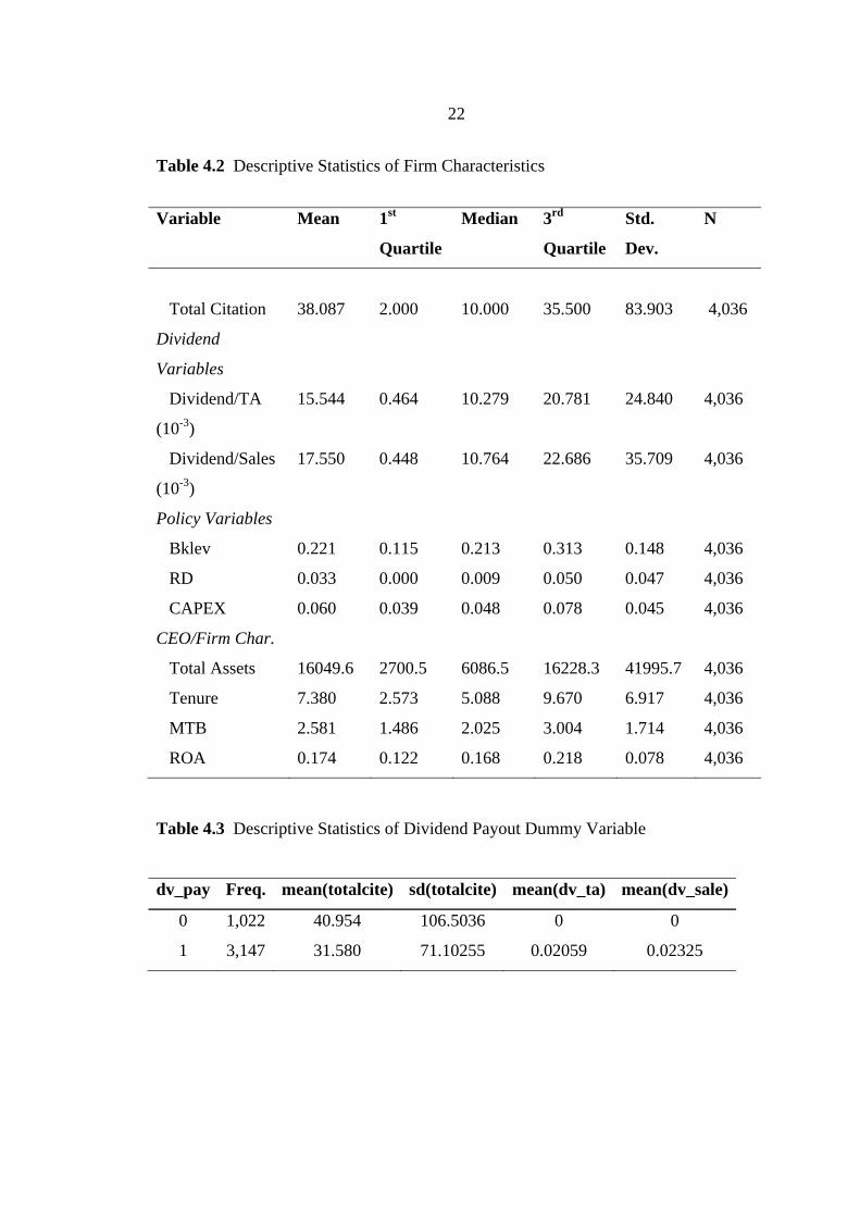
Table 4.2 and Table 4.3 report on the statistics of the major variables. The
reputation variable (as measured by the total number of media cites) was highly
21
skewed. This study adopted the method to fix this in the later analysis by taking the
logarithm of the number of citations plus unity. Dividend payout in the tobit
regression was measured by annual dividend divided by total assets and dividend
divided by sales.
Firm policy variables included investment variables (capital expenditure, book
leverage, and R&D investment). Finally, the main CEO/firm characteristic variables
that were used for the tests included total assets (firm size), CEO tenure, and market-
to-book value ratio. A few observations are noteworthy. On average, the CEO has
been in office for 7.38 years. The average R&D spending was 3.3% of total assets;
however, the capital expenditure was almost twice of R&D spending. The average
market-to-book value ratio was about 2.58 times, and the sample firms were on
average financially healthy, as suggested by the average ROA of 17.4%.
The sample consisted of CEOs of all S&P 500 firms as identified from the
Execucomp database over the period 1992-2007. The total citation was the number of
articles containing the CEO’s full name and company affiliation that appeared in
major U.S. and global newspapers and newswires in calendar year t.
Dividend/Total Assets was calculated by annual dividend divided by the
ending total assets in year t. Dividend/Sales was obtained by dividing the annual
dividend by annual sales. The Bklev was the ratio of long-term debt plus debt in
current liabilities to the book value of assets (TA) in year t.
Total Assets was the book value of assets in year t (TA). Tenure was the
number of years that the CEO had served in that capacity, as reported in the
Execucomp in year t. The MTB was the ratio of the market value of assets to the book
value of assets. Bklev was the ratio of long-term debt plus debt in current liabilities to
total assets.
The RD was the research and development expenses (RD) scaled by TA.
Missing RD was set to zero. CAPEX was the capital expenditure (CAPEX) scaled by
total assets. ROA was the ratio of operating income before depreciation to book assets
(OIBDP/TA). All variables were winsorized at the 1% and 99% level.
22
Table 4.2 Descriptive Statistics of Firm Characteristics
Variable Mean 1st
Quartile
Median 3rd
Quartile
Std.
Dev.
N
Total Citation
38.087
2.000
10.000
35.500
83.903
4,036
Dividend
Variables
Dividend/TA
(10-3)
15.544 0.464 10.279 20.781 24.840 4,036
Dividend/Sales
(10-3)
17.550 0.448 10.764 22.686 35.709 4,036
Policy Variables
Bklev 0.221 0.115 0.213 0.313 0.148 4,036
RD 0.033 0.000 0.009 0.050 0.047 4,036
CAPEX 0.060 0.039 0.048 0.078 0.045 4,036
CEO/Firm Char.
Total Assets 16049.6 2700.5 6086.5 16228.3 41995.7 4,036
Tenure 7.380 2.573 5.088 9.670 6.917 4,036
MTB 2.581 1.486 2.025 3.004 1.714 4,036
ROA 0.174 0.122 0.168 0.218 0.078 4,036
Table 4.3 Descriptive Statistics of Dividend Payout Dummy Variable
dv_pay Freq. mean(totalcite) sd(totalcite) mean(dv_ta) mean(dv_sale)
0 1,022 40.954 106.5036 0 0
1 3,147 31.580 71.10255 0.02059 0.02325
CHAPTER 5
METHODOLOGY
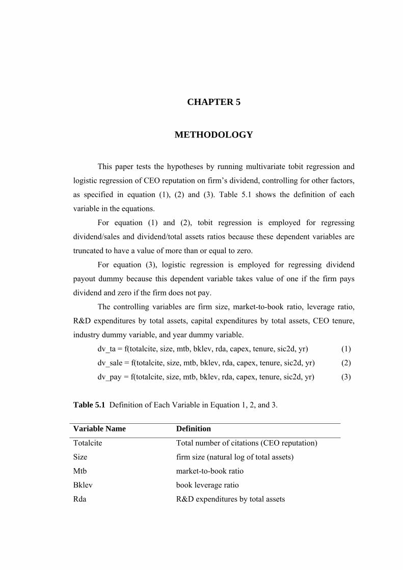
This paper tests the hypotheses by running multivariate tobit regression and
logistic regression of CEO reputation on firm’s dividend, controlling for other factors,
as specified in equation (1), (2) and (3). Table 5.1 shows the definition of each
variable in the equations.
For equation (1) and (2), tobit regression is employed for regressing
dividend/sales and dividend/total assets ratios because these dependent variables are
truncated to have a value of more than or equal to zero.
For equation (3), logistic regression is employed for regressing dividend
payout dummy because this dependent variable takes value of one if the firm pays
dividend and zero if the firm does not pay.
The controlling variables are firm size, market-to-book ratio, leverage ratio,
R&D expenditures by total assets, capital expenditures by total assets, CEO tenure,
industry dummy variable, and year dummy variable.
dv_ta = f(totalcite, size, mtb, bklev, rda, capex, tenure, sic2d, yr) (1)
dv_sale = f(totalcite, size, mtb, bklev, rda, capex, tenure, sic2d, yr) (2)
dv_pay = f(totalcite, size, mtb, bklev, rda, capex, tenure, sic2d, yr) (3)
Table 5.1 Definition of Each Variable in Equation 1, 2, and 3.
Variable Name Definition
Totalcite Total number of citations (CEO reputation)
Size firm size (natural log of total assets)
Mtb market-to-book ratio
Bklev book leverage ratio
Rda R&D expenditures by total assets
24
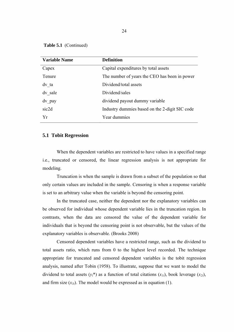
Table 5.1 (Continued)
Variable Name Definition
Capex Capital expenditures by total assets
Tenure The number of years the CEO has been in power
dv_ta Dividend/total assets
dv_sale Dividend/sales
dv_pay dividend payout dummy variable
sic2d Industry dummies based on the 2-digit SIC code
Yr Year dummies
5.1 Tobit Regression
When the dependent variables are restricted to have values in a specified range
i.e., truncated or censored, the linear regression analysis is not appropriate for
modeling.
Truncation is when the sample is drawn from a subset of the population so that
only certain values are included in the sample. Censoring is when a response variable
is set to an arbitrary value when the variable is beyond the censoring point.
In the truncated case, neither the dependent nor the explanatory variables can
be observed for individual whose dependent variable lies in the truncation region. In
contrasts, when the data are censored the value of the dependent variable for
individuals that is beyond the censoring point is not observable, but the values of the
explanatory variables is observable. (Brooks 2008)
Censored dependent variables have a restricted range, such as the dividend to
total assets ratio, which runs from 0 to the highest level recorded. The technique
appropriate for truncated and censored dependent variables is the tobit regression
analysis, named after Tobin (1958). To illustrate, suppose that we want to model the
dividend to total assets (yi*) as a function of total citations (x1i), book leverage (x2i),
and firm size (x3i). The model would be expressed as in equation (1).
25
yi* = b0 + b1x1i + b2x2i + b3x3i + ei (1)
yi = yi* for yi* ≥ 0
yi = 0 for yi* < 0
yi* represents the true dividend to total assets and this will be observable only
for dividend to total assets more than or equal to zero.
In this study, tobit regression analysis is employed for the models whose
dependent variables are dividend to total assets and dividend to sales because these
two variables are left censored at zero.
5.2 Logistic Regression
Logistic regression analysis is a nonlinear regression model widely used when
the response variable is qualitative. For example, if we want to predict whether the
firm is going to payout dividend or not. In this use of logistic regression model, the
response variable is qualitative and will be represented by a 0, 1 indicator variable.
(Kutner, Nachtsheim, Neter, and Li 2005)
The parameters of the Logistic response function are estimated by using the
method of maximum likelihood because this method is well suited to deal with the
problems associated with the responses variable being binary. The logistic regression
assumes that the logit transformation of the outcome variable has a linear relationship
with the predictor variables. The logistic regression model in the usual form is
expressed in equation (2).
yi = E[yi] + ei (2)
yi are independent Bernoulli random variables with expected values in
equation (3).
E[yi] = exp(b0 + b1x1i + b2x2i + b3x3i) / (1 + exp(b0 + b1x1i + b2x2i + b3x3i)) (3)
Since each yi observation is an ordinary Bernoulli random variable, where:
P(yi = 1) = ∏i
P(yi = 0) = 1 – ∏i
The maximum likelihood estimates of coefficients in the logistic regression
model will be those values of coefficients that maximize the log-likelihood function.
26
The logistic estimation can be transform into the log of odds ratio which is
expressed as in equation (4).
Log (∏i / 1 – ∏i) = b0 + b1x1i (4)
The left hand of the equation (4) above is known as the odds ratio which
expresses the probability in terms of the odds of y = 1.
The interpretation of the estimated regression coefficient (bi) in the logistic
response function is, assuming all other variables are held constant, for any unit
increase in x1, the estimated ratio of the odds is exp(bi). (Baum 2006)
For example, if the b1 is 1.2, then it means for any unit increase in x1, the log
of odds will be 1.2, the odds ratio will be equal to exp(1.2) which is 3.32. and the
probability that the observation will fall into a specified category can be computed
from p/(1 – p) = 3.32 so the probability will be equal to 0.7685.
In this study, suppose that we want to model the propensity of the firm to
payout dividend (yi*) as a function of total citations (x1i), book leverage (x2i), and firm
size (x3i). The model would be expressed as in equation (2) and equation (3) where the
propensity to payout (yi*) is a function of total citations (x1i), book leverage (x2i), and
firm size (x3i).
If the estimated logit regression coefficient of total citations equal to -0.5, then
it can be interpreted as, assuming all other variables are held constant, for any unit
increase in total citations, the estimated ratio of the odds of paying out dividend for
firm is equal to exp(-0.5) which is 0.6065. And this odds can be transformed to the
expected probability (or propensity) that the firm will pay dividend equal to 0.3775.
CHAPTER 6
RESULTS
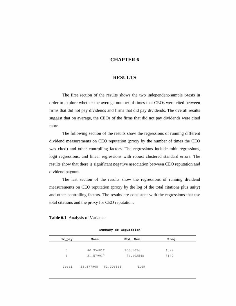
The first section of the results shows the two independent-sample t-tests in
order to explore whether the average number of times that CEOs were cited between
firms that did not pay dividends and firms that did pay dividends. The overall results
suggest that on average, the CEOs of the firms that did not pay dividends were cited
more.
The following section of the results show the regressions of running different
dividend measurements on CEO reputation (proxy by the number of times the CEO
was cited) and other controlling factors. The regressions include tobit regressions,
logit regressions, and linear regressions with robust clustered standard errors. The
results show that there is significant negative association between CEO reputation and
dividend payouts.
The last section of the results show the regressions of running dividend
measurements on CEO reputation (proxy by the log of the total citations plus unity)
and other controlling factors. The results are consistent with the regressions that use
total citations and the proxy for CEO reputation.
Table 6.1 Analysis of Variance
Summary of Reputation
dv_pay Mean Std. Dev. Freq.
0 40.954012 106.5036 1022
1 31.579917 71.102548 3147
Total 33.877908 81.306868 4169
28
Table 6.1 (Continued)
Analysis of Variance
Source SS df MS F Prob > F
Between groups 67791.366 1 67791.366 10.28 0.0014
Within groups 27486051.5 4167 6596.12467
Total 27553842.9 4168 6610.80683
Note: Bartlett's test for equal variances:
chi2(1) = 283.2040 Prob>chi2 = 0.000
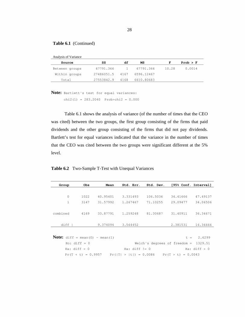
Table 6.1 shows the analysis of variance (of the number of times that the CEO
was cited) between the two groups, the first group consisting of the firms that paid
dividends and the other group consisting of the firms that did not pay dividends.
Bartlett’s test for equal variances indicated that the variance in the number of times
that the CEO was cited between the two groups were significant different at the 5%
level.
Table 6.2 Two-Sample T-Test with Unequal Variances
Group Obs Mean Std. Err. Std. Dev. [95% Conf. Interval]
0 1022 40.95401 3.331493 106.5036 34.41666 47.49137
1 3147 31.57992 1.267467 71.10255 29.09477 34.06506
combined 4169 33.87791 1.259248 81.30687 31.40911 36.34671
diff | 9.374094 3.564452 2.381531 16.36666
Note: diff = mean(0) - mean(1) t = 2.6299 Ho: diff = 0 Welch's degrees of freedom = 1329.51
Ha: diff < 0 Ha: diff != 0 Ha: diff > 0
Pr(T < t) = 0.9957 Pr(|T| > |t|) = 0.0086 Pr(T > t) = 0.0043
29
Table 6.2 shows the two-sample t-tests of the mean equality between group 0
(firms that did not pay dividends) and group 1 (firms that paid dividends). The
average number of times that the CEOs of firms that did not pay dividends were cited
was approximately 41 times, whereas the average number of times that the CEOs of
the firms that did pay dividends were cited was approximately 32 times. The Welch’s
statistic shows that, on average, the CEOs of firms that did not pay out dividends were
cited more that the CEOs of firms that paid dividends. These results imply that the
regressions of dividend payout variables on the number of times that the CEO was
cited should report a negative association.
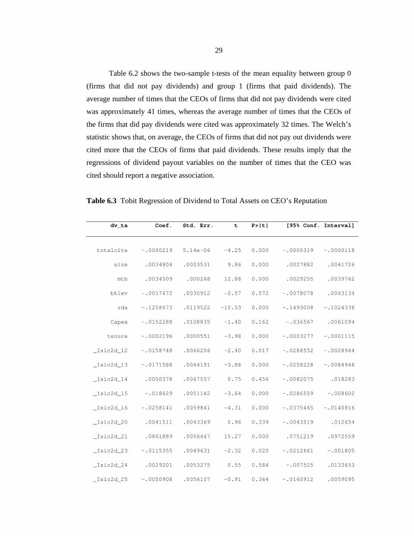
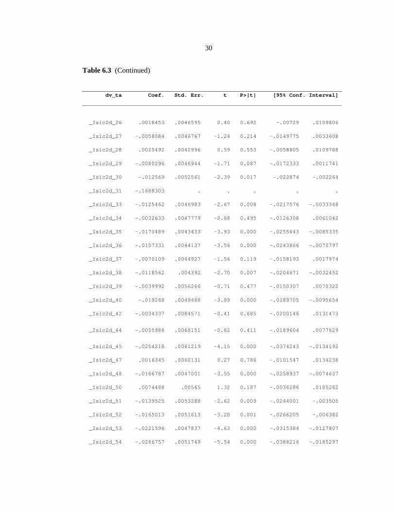
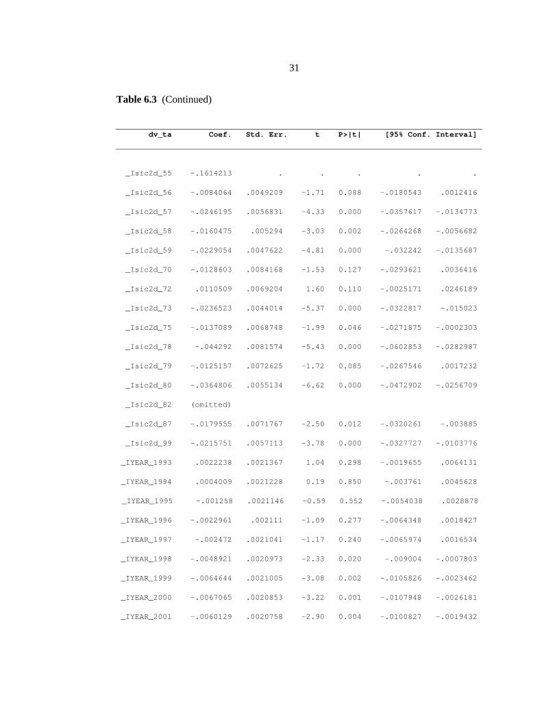
Table 6.3 Tobit Regression of Dividend to Total Assets on CEO’s Reputation
dv_ta Coef. Std. Err. t P>|t| [95% Conf. Interval]
totalcite -.0000219 5.14e-06 -4.25 0.000 -.0000319 -.0000118
size .0034804 .0003531 9.86 0.000 .0027882 .0041726
mtb .0034509 .000268 12.88 0.000 .0029255 .0039762
bklev -.0017472 .0030912 -0.57 0.572 -.0078078 .0043134
rda -.1258673 .0119522 -10.53 0.000 -.1493008 -.1024338
Capex -.0152288 .0108835 -1.40 0.162 -.036567 .0061094
tenure -.0002196 .0000551 -3.98 0.000 -.0003277 -.0001115
_Isic2d_12 -.0158748 .0066206 -2.40 0.017 -.0288552 -.0028944
_Isic2d_13 -.0171588 .0044191 -3.88 0.000 -.0258228 -.0084948
_Isic2d_14 .0050378 .0067557 0.75 0.456 -.0082075 .018283
_Isic2d_15 -.018629 .0051142 -3.64 0.000 -.0286559 -.008602
_Isic2d_16 -.0258141 .0059841 -4.31 0.000 -.0375465 -.0140816
_Isic2d_20 .0041511 .0043369 0.96 0.339 -.0043519 .012654
_Isic2d_21 .0861889 .0056447 15.27 0.000 .0751219 .0972559
_Isic2d_23 -.0115355 .0049631 -2.32 0.020 -.0212661 -.001805
_Isic2d_24 .0029201 .0053275 0.55 0.584 -.007525 .0133653
_Isic2d_25 -.0050908 .0056107 -0.91 0.364 -.0160912 .0059095
30
Table 6.3 (Continued)
dv_ta Coef. Std. Err. t P>|t| [95% Conf. Interval]
_Isic2d_26 .0018453 .0046595 0.40 0.692 -.00729 .0109806
_Isic2d_27 -.0058084 .0046767 -1.24 0.214 -.0149775 .0033608
_Isic2d_28 .0025492 .0042996 0.59 0.553 -.0058805 .0109788
_Isic2d_29 -.0080296 .0046944 -1.71 0.087 -.0172333 .0011741
_Isic2d_30 -.012569 .0052561 -2.39 0.017 -.022874 -.002264
_Isic2d_31 -.1688303 . . . . .
_Isic2d_33 -.0125462 .0046983 -2.67 0.008 -.0217576 -.0033348
_Isic2d_34 -.0032633 .0047779 -0.68 0.495 -.0126308 .0061042
_Isic2d_35 -.0170489 .0043433 -3.93 0.000 -.0255643 -.0085335
_Isic2d_36 -.0157331 .0044137 -3.56 0.000 -.0243866 -.0070797
_Isic2d_37 -.0070109 .0044927 -1.56 0.119 -.0158193 .0017974
_Isic2d_38 -.0118562 .004392 -2.70 0.007 -.0204671 -.0032452
_Isic2d_39 -.0039992 .0056266 -0.71 0.477 -.0150307 .0070322
_Isic2d_40 -.019268 .0049488 -3.89 0.000 -.0289705 -.0095654
_Isic2d_42 -.0034337 .0084571 -0.41 0.685 -.0200146 .0131473
_Isic2d_44 -.0055988 .0068151 -0.82 0.411 -.0189604 .0077629
_Isic2d_45 -.0254218 .0061219 -4.15 0.000 -.0374243 -.0134192
_Isic2d_47 .0016345 .0060131 0.27 0.786 -.0101547 .0134238
_Isic2d_48 -.0166787 .0047001 -3.55 0.000 -.0258937 -.0074637
_Isic2d_50 .0074488 .00565 1.32 0.187 -.0036286 .0185262
_Isic2d_51 -.0139525 .0053288 -2.62 0.009 -.0244001 -.003505
_Isic2d_52 -.0165013 .0051613 -3.20 0.001 -.0266205 -.006382
_Isic2d_53 -.0221596 .0047837 -4.63 0.000 -.0315384 -.0127807
_Isic2d_54 -.0286757 .0051749 -5.54 0.000 -.0388216 -.0185297
31
Table 6.3 (Continued)
dv_ta Coef. Std. Err. t P>|t| [95% Conf. Interval]
_Isic2d_55 -.1614213 . . . . .
_Isic2d_56 -.0084064 .0049209 -1.71 0.088 -.0180543 .0012416
_Isic2d_57 -.0246195 .0056831 -4.33 0.000 -.0357617 -.0134773
_Isic2d_58 -.0160475 .005294 -3.03 0.002 -.0264268 -.0056682
_Isic2d_59 -.0229054 .0047622 -4.81 0.000 -.032242 -.0135687
_Isic2d_70 -.0128603 .0084168 -1.53 0.127 -.0293621 .0036416
_Isic2d_72 .0110509 .0069204 1.60 0.110 -.0025171 .0246189
_Isic2d_73 -.0236523 .0044014 -5.37 0.000 -.0322817 -.015023
_Isic2d_75 -.0137089 .0068748 -1.99 0.046 -.0271875 -.0002303
_Isic2d_78 -.044292 .0081574 -5.43 0.000 -.0602853 -.0282987
_Isic2d_79 -.0125157 .0072625 -1.72 0.085 -.0267546 .0017232
_Isic2d_80 -.0364806 .0055134 -6.62 0.000 -.0472902 -.0256709
_Isic2d_82 (omitted)
_Isic2d_87 -.0179555 .0071767 -2.50 0.012 -.0320261 -.003885
_Isic2d_99 -.0215751 .0057113 -3.78 0.000 -.0327727 -.0103776
_IYEAR_1993 .0022238 .0021367 1.04 0.298 -.0019655 .0064131
_IYEAR_1994 .0004009 .0021228 0.19 0.850 -.003761 .0045628
_IYEAR_1995 -.001258 .0021146 -0.59 0.552 -.0054038 .0028878
_IYEAR_1996 -.0022961 .002111 -1.09 0.277 -.0064348 .0018427
_IYEAR_1997 -.002472 .0021041 -1.17 0.240 -.0065974 .0016534
_IYEAR_1998 -.0048921 .0020973 -2.33 0.020 -.009004 -.0007803
_IYEAR_1999 -.0064644 .0021005 -3.08 0.002 -.0105826 -.0023462
_IYEAR_2000 -.0067065 .0020853 -3.22 0.001 -.0107948 -.0026181
_IYEAR_2001 -.0060129 .0020758 -2.90 0.004 -.0100827 -.0019432
32
Table 6.3 (Continued)
dv_ta Coef. Std. Err. t P>|t| [95% Conf. Interval]
_IYEAR_2002 -.0072114 .0020678 -3.49 0.000 -.0112655 -.0031573
_IYEAR_2003 -.0072783 .002066 -3.52 0.000 -.0113288 -.0032277
_IYEAR_2004 -.0061334 .0020539 -2.99 0.003 -.0101602 -.0021066
_IYEAR_2005 -.0038004 .0020488 -1.85 0.064 -.0078172 .0002164
_IYEAR_2006 .0002162 .0020875 0.10 0.918 -.0038764 .0043089
_cons -.0051764 .0054668 -0.95 0.344 -.0158946 .0055418
/sigma | .0207618 .0002798 .0202131 .0213104
Note: 1. . xi: tobit dv_ta totalcite size mtb bklev rda Capex
tenure i.sic2d i.YEAR, ll(0)
i.sic2d _Isic2d_10-99 (naturally coded; _Isic2d_10 omitted)
i.YEAR _IYEAR_1992-2006 (naturally coded; _IYEAR_1992 omitted)
2. _Isic2d_82 omitted because of collinearity
Tobit regression Number of obs = 3834
LR chi2(67) = 1839.75
Prob > chi2 = 0.0000
Log likelihood = 6594.2896 Pseudo R2 = -0.1621
3. Obs. summary: 900 left-censored observations at dv_ta<=0
2934 uncensored observations
0 right-censored observations
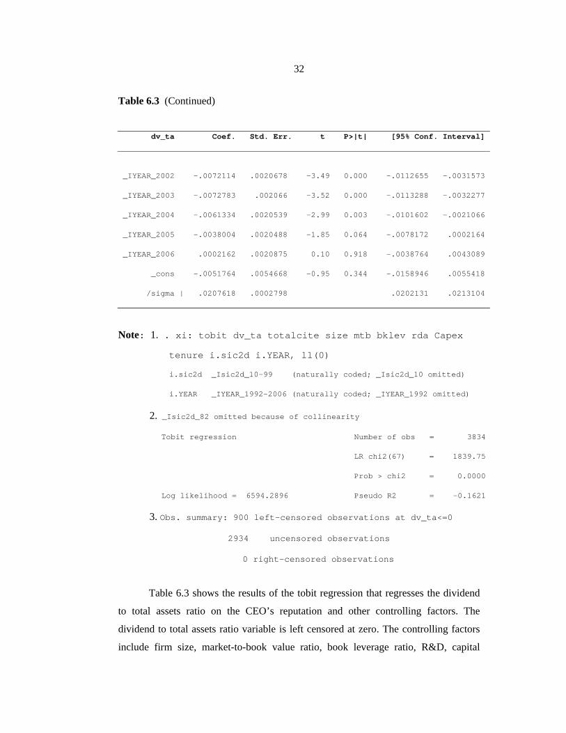
Table 6.3 shows the results of the tobit regression that regresses the dividend
to total assets ratio on the CEO’s reputation and other controlling factors. The
dividend to total assets ratio variable is left censored at zero. The controlling factors
include firm size, market-to-book value ratio, book leverage ratio, R&D, capital
33
expenditures, CEO tenure, and also the industry SIC code and year dummies. At 5%
level of significant, the tobit estimates of dividend to total assets ratio show negative,
significant effects regarding the CEO’s reputation. The results imply that the increase
in CEO’s reputation is associated with the decrease in probability that the firm will
pay more dividends in relation to the percentage of its total assets. At 5% level of
significant, the tobit estimates also reveal negative significant effects regarding the
R&D expenditures. These results support the investment hypothesis, which predicts
that reputable CEOs tend to use funds to invest more rather than paying out dividends.
For the controlling variables, the results show that firm size and market-to-
book value ratio have a significant positive association with the dividend to total
assets ratio (at the 5% significance level). However, firm R&D expenditures and CEO
tenure exhibited a significant negative association with dividend to total assets ratio
(at the 5% significance level). The firm book leverage and capital expenditures had an
insignificant association with dividend to total assets ratio.
The significant negative association between firm R&D and dividend to total
assets ratio shows that the firm that invests more in R&D tends to pay lower
dividends. It also supports the investment hypothesis whereby reputable CEOs pay
fewer dividends because they use the available internal funds to make more R&D
expenditures, which implies that reputable CEOs tend to be more confident that their
investments will turn out to be successful.
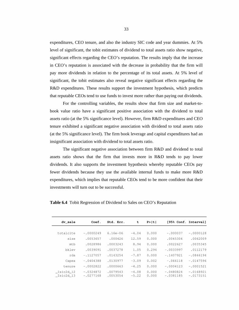
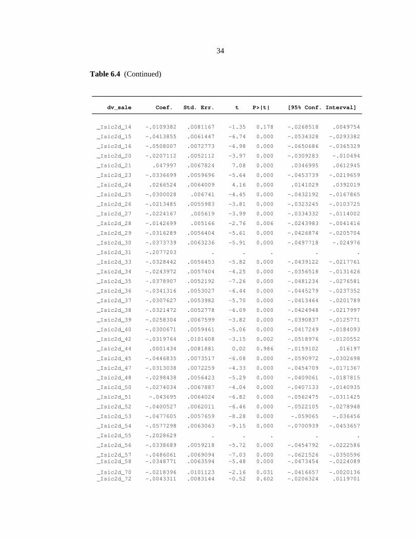
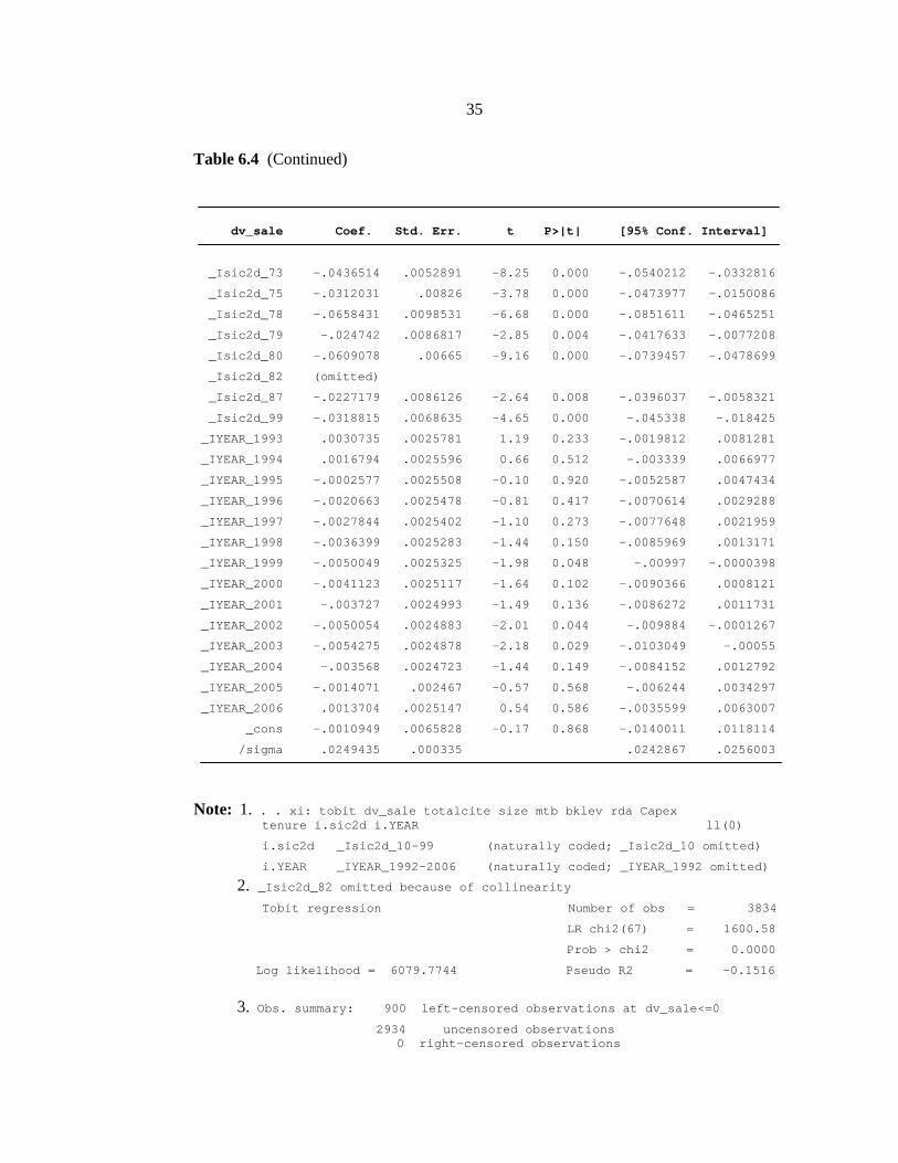
Table 6.4 Tobit Regression of Dividend to Sales on CEO’s Reputation
dv_sale Coef. Std. Err. t P>|t| [95% Conf. Interval]
totalcite -.0000249 6.16e-06 -4.04 0.000 -.000037 -.0000128
size .0053657 .000426 12.59 0.000 .0045304 .0062009
mtb .0028986 .0003243 8.94 0.000 .0022627 .0035345
bklev .0039091 .0037278 1.05 0.294 -.0033997 .0112179
rda -.1127057 .0143254 -7.87 0.000 -.1407921 -.0846194
Capex -.0404388 .0130977 -3.09 0.002 -.066118 -.0147596
tenure -.0002822 .0000663 -4.25 0.000 -.0004123 -.0001521
_Isic2d_12 -.0324872 .0079543 -4.08 0.000 -.0480824 -.0168921 _Isic2d_13 -.0277168 .0053054 -5.22 0.000 -.0381185 -.0173151
34
Table 6.4 (Continued) dv_sale Coef. Std. Err. t P>|t| [95% Conf. Interval]
_Isic2d_14 -.0109382 .0081167 -1.35 0.178 -.0268518 .0049754
_Isic2d_15 -.0413855 .0061447 -6.74 0.000 -.0534328 -.0293382
_Isic2d_16 -.0508007 .0072773 -6.98 0.000 -.0650686 -.0365329
_Isic2d_20 -.0207112 .0052112 -3.97 0.000 -.0309283 -.010494
_Isic2d_21 .047997 .0067824 7.08 0.000 .0346995 .0612945
_Isic2d_23 -.0336699 .0059696 -5.64 0.000 -.0453739 -.0219659
_Isic2d_24 .0266524 .0064009 4.16 0.000 .0141029 .0392019
_Isic2d_25 -.0300028 .006741 -4.45 0.000 -.0432192 -.0167865
_Isic2d_26 -.0213485 .0055983 -3.81 0.000 -.0323245 -.0103725
_Isic2d_27 -.0224167 .005619 -3.99 0.000 -.0334332 -.0114002
_Isic2d_28 -.0142699 .005166 -2.76 0.006 -.0243983 -.0041416
_Isic2d_29 -.0316289 .0056404 -5.61 0.000 -.0426874 -.0205704
_Isic2d_30 -.0373739 .0063236 -5.91 0.000 -.0497718 -.024976
_Isic2d_31 -.2077203 . . . . .
_Isic2d_33 -.0328442 .0056453 -5.82 0.000 -.0439122 -.0217761
_Isic2d_34 -.0243972 .0057404 -4.25 0.000 -.0356518 -.0131426
_Isic2d_35 -.0378907 .0052192 -7.26 0.000 -.0481234 -.0276581
_Isic2d_36 -.0341316 .0053027 -6.44 0.000 -.0445279 -.0237352
_Isic2d_37 -.0307627 .0053982 -5.70 0.000 -.0413464 -.0201789
_Isic2d_38 -.0321472 .0052778 -6.09 0.000 -.0424948 -.0217997
_Isic2d_39 -.0258304 .0067599 -3.82 0.000 -.0390837 -.0125771
_Isic2d_40 -.0300671 .0059461 -5.06 0.000 -.0417249 -.0184093
_Isic2d_42 -.0319764 .0101608 -3.15 0.002 -.0518976 -.0120552
_Isic2d_44 .0001434 .0081881 0.02 0.986 -.0159102 .016197
_Isic2d_45 -.0446835 .0073517 -6.08 0.000 -.0590972 -.0302698
_Isic2d_47 -.0313038 .0072259 -4.33 0.000 -.0454709 -.0171367
_Isic2d_48 -.0298438 .0056423 -5.29 0.000 -.0409061 -.0187815
_Isic2d_50 -.0274034 .0067887 -4.04 0.000 -.0407133 -.0140935
_Isic2d_51 -.043695 .0064024 -6.82 0.000 -.0562475 -.0311425
_Isic2d_52 -.0400527 .0062011 -6.46 0.000 -.0522105 -.0278948
_Isic2d_53 -.0477605 .0057659 -8.28 0.000 -.059065 -.036456
_Isic2d_54 -.0577298 .0063063 -9.15 0.000 -.0700939 -.0453657
_Isic2d_55 -.2028629 . . . . .
_Isic2d_56 -.0338689 .0059218 -5.72 0.000 -.0454792 -.0222586
_Isic2d_57 -.0486061 .0069094 -7.03 0.000 -.0621526 -.0350596 _Isic2d_58 -.0348771 .0063594 -5.48 0.000 -.0473454 -.0224089
_Isic2d_70 -.0218396 .0101123 -2.16 0.031 -.0416657 -.0020136 _Isic2d_72 -.0043311 .0083144 -0.52 0.602 -.0206324 .0119701
35
Table 6.4 (Continued) dv_sale Coef. Std. Err. t P>|t| [95% Conf. Interval]
_Isic2d_73 -.0436514 .0052891 -8.25 0.000 -.0540212 -.0332816
_Isic2d_75 -.0312031 .00826 -3.78 0.000 -.0473977 -.0150086
_Isic2d_78 -.0658431 .0098531 -6.68 0.000 -.0851611 -.0465251
_Isic2d_79 -.024742 .0086817 -2.85 0.004 -.0417633 -.0077208
_Isic2d_80 -.0609078 .00665 -9.16 0.000 -.0739457 -.0478699
_Isic2d_82 (omitted)
_Isic2d_87 -.0227179 .0086126 -2.64 0.008 -.0396037 -.0058321
_Isic2d_99 -.0318815 .0068635 -4.65 0.000 -.045338 -.018425
_IYEAR_1993 .0030735 .0025781 1.19 0.233 -.0019812 .0081281
_IYEAR_1994 .0016794 .0025596 0.66 0.512 -.003339 .0066977
_IYEAR_1995 -.0002577 .0025508 -0.10 0.920 -.0052587 .0047434
_IYEAR_1996 -.0020663 .0025478 -0.81 0.417 -.0070614 .0029288
_IYEAR_1997 -.0027844 .0025402 -1.10 0.273 -.0077648 .0021959
_IYEAR_1998 -.0036399 .0025283 -1.44 0.150 -.0085969 .0013171
_IYEAR_1999 -.0050049 .0025325 -1.98 0.048 -.00997 -.0000398
_IYEAR_2000 -.0041123 .0025117 -1.64 0.102 -.0090366 .0008121
_IYEAR_2001 -.003727 .0024993 -1.49 0.136 -.0086272 .0011731
_IYEAR_2002 -.0050054 .0024883 -2.01 0.044 -.009884 -.0001267
_IYEAR_2003 -.0054275 .0024878 -2.18 0.029 -.0103049 -.00055
_IYEAR_2004 -.003568 .0024723 -1.44 0.149 -.0084152 .0012792
_IYEAR_2005 -.0014071 .002467 -0.57 0.568 -.006244 .0034297
_IYEAR_2006 .0013704 .0025147 0.54 0.586 -.0035599 .0063007
_cons -.0010949 .0065828 -0.17 0.868 -.0140011 .0118114
/sigma .0249435 .000335 .0242867 .0256003
Note: 1. . . xi: tobit dv_sale totalcite size mtb bklev rda Capex tenure i.sic2d i.YEAR ll(0)
i.sic2d _Isic2d_10-99 (naturally coded; _Isic2d_10 omitted)
i.YEAR _IYEAR_1992-2006 (naturally coded; _IYEAR_1992 omitted)
2. _Isic2d_82 omitted because of collinearity Tobit regression Number of obs = 3834
LR chi2(67) = 1600.58
Prob > chi2 = 0.0000
Log likelihood = 6079.7744 Pseudo R2 = -0.1516
3. Obs. summary: 900 left-censored observations at dv_sale<=0
2934 uncensored observations 0 right-censored observations
36
Table 6.4 shows the results of the tobit regression, which regress the dividend
to sales ratio on the CEO’s reputation and other controlling factors. The dividend to
sales ratio variable is left censored at zero. Similar to the previous regression (the
regression of dividend to total assets ratio and the CEO’s reputation in Table 6.3), this
tobit estimate of dividend to sales ratio shows negative, significant effects regarding
the CEO’s reputation. The results imply that the CEO’s reputation decreases the
probability that the firm will pay more dividends in relation to the percentage of its
sales. These results also support the investment hypothesis, which predicts that
reputable CEOs tend funds to make more investments rather than to payout dividends.
For the controlling variables, the results show that firm size and the market-to-
book value ratio have a significant positive association with the dividend to sales ratio
(at the 5% significance level). However, firm R&D expenditures, capital
expenditures, and CEO tenure exhibited a significant negative association with the
dividend to sales ratio (at the 5% significance level). The firm book leverage was the
only factor that had an insignificant association with the dividend to sales ratio.
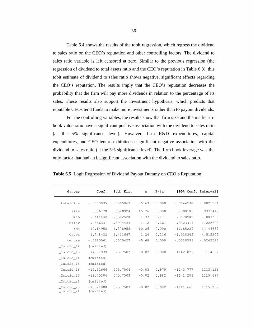
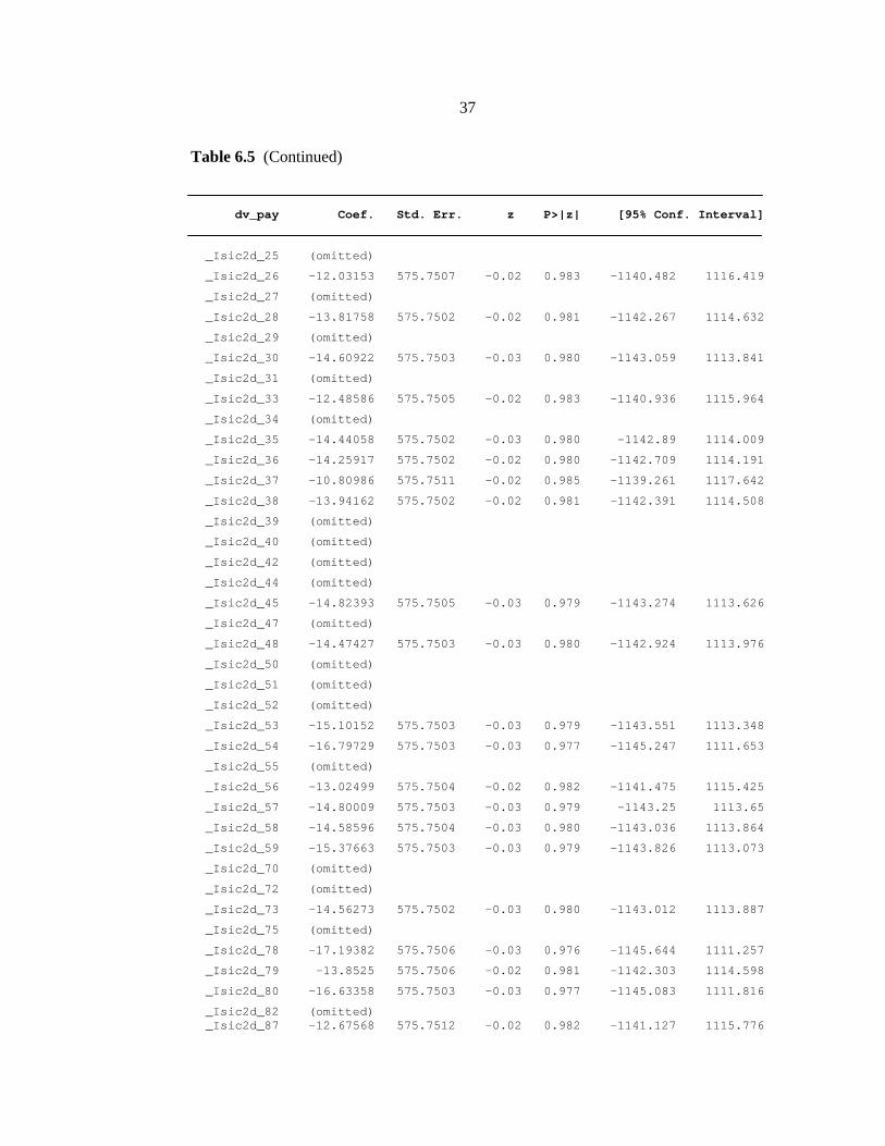
Table 6.5 Logit Regression of Dividend Payout Dummy on CEO’s Reputation
dv_pay Coef. Std. Err. z P>|z| [95% Conf. Interval]
totalcite -.0033035 .0005869 -5.63 0.000 -.0044538 -.0021531 size .8336778 .0528924 15.76 0.000 .7300106 .9373449
mtb .0414442 .0302528 1.37 0.171 -.0178502 .1007386
bklev .4466331 .3974434 1.12 0.261 -.3323417 1.225608
rda -14.14958 1.378958 -10.26 0.000 -16.85229 -11.44687
Capex 1.748432 1.411647 1.24 0.216 -1.018345 4.515209
tenure -.0380561 .0070427 -5.40 0.000 -.0518596 -.0242526
_Isic2d_12 (omitted)
_Isic2d_13 -14.37939 575.7502 -0.02 0.980 -1142.829 1114.07
_Isic2d_14 (omitted)
_Isic2d_15 (omitted)
_Isic2d_16 -15.32666 575.7504 -0.03 0.979 -1143.777 1113.123
_Isic2d_20 -12.75304 575.7503 -0.02 0.982 -1141.203 1115.697
_Isic2d_21 (omitted)
_Isic2d_23 -13.21088 575.7503 -0.02 0.982 -1141.661 1115.239 _Isic2d_24 (omitted)
37
Table 6.5 (Continued)
dv_pay Coef. Std. Err. z P>|z| [95% Conf. Interval]
_Isic2d_25 (omitted)
_Isic2d_26 -12.03153 575.7507 -0.02 0.983 -1140.482 1116.419
_Isic2d_27 (omitted)
_Isic2d_28 -13.81758 575.7502 -0.02 0.981 -1142.267 1114.632
_Isic2d_29 (omitted)
_Isic2d_30 -14.60922 575.7503 -0.03 0.980 -1143.059 1113.841
_Isic2d_31 (omitted)
_Isic2d_33 -12.48586 575.7505 -0.02 0.983 -1140.936 1115.964
_Isic2d_34 (omitted)
_Isic2d_35 -14.44058 575.7502 -0.03 0.980 -1142.89 1114.009
_Isic2d_36 -14.25917 575.7502 -0.02 0.980 -1142.709 1114.191
_Isic2d_37 -10.80986 575.7511 -0.02 0.985 -1139.261 1117.642
_Isic2d_38 -13.94162 575.7502 -0.02 0.981 -1142.391 1114.508
_Isic2d_39 (omitted)
_Isic2d_40 (omitted)
_Isic2d_42 (omitted)
_Isic2d_44 (omitted)
_Isic2d_45 -14.82393 575.7505 -0.03 0.979 -1143.274 1113.626
_Isic2d_47 (omitted)
_Isic2d_48 -14.47427 575.7503 -0.03 0.980 -1142.924 1113.976
_Isic2d_50 (omitted)
_Isic2d_51 (omitted)
_Isic2d_52 (omitted)
_Isic2d_53 -15.10152 575.7503 -0.03 0.979 -1143.551 1113.348
_Isic2d_54 -16.79729 575.7503 -0.03 0.977 -1145.247 1111.653
_Isic2d_55 (omitted)
_Isic2d_56 -13.02499 575.7504 -0.02 0.982 -1141.475 1115.425
_Isic2d_57 -14.80009 575.7503 -0.03 0.979 -1143.25 1113.65
_Isic2d_58 -14.58596 575.7504 -0.03 0.980 -1143.036 1113.864
_Isic2d_59 -15.37663 575.7503 -0.03 0.979 -1143.826 1113.073
_Isic2d_70 (omitted)
_Isic2d_72 (omitted)
_Isic2d_73 -14.56273 575.7502 -0.03 0.980 -1143.012 1113.887
_Isic2d_75 (omitted)
_Isic2d_78 -17.19382 575.7506 -0.03 0.976 -1145.644 1111.257
_Isic2d_79 -13.8525 575.7506 -0.02 0.981 -1142.303 1114.598
_Isic2d_80 -16.63358 575.7503 -0.03 0.977 -1145.083 1111.816
_Isic2d_82 (omitted) _Isic2d_87 -12.67568 575.7512 -0.02 0.982 -1141.127 1115.776
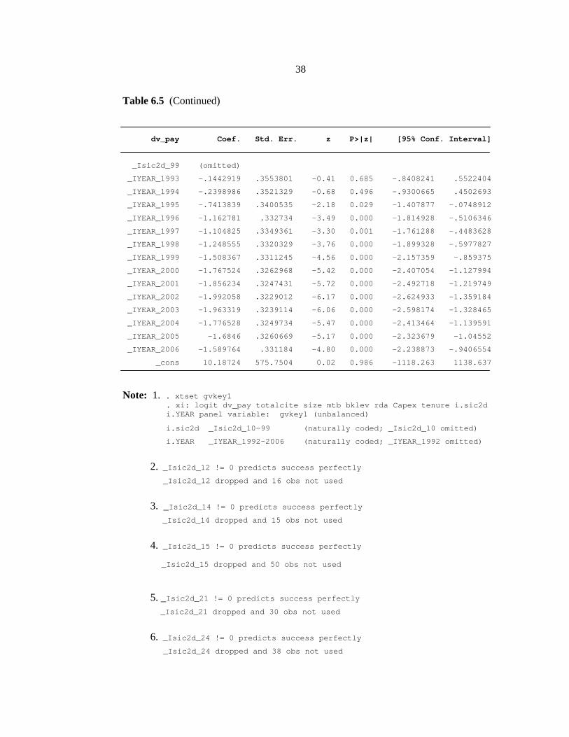
38
Table 6.5 (Continued)
dv_pay Coef. Std. Err. z P>|z| [95% Conf. Interval]
_Isic2d_99 (omitted)
_IYEAR_1993 -.1442919 .3553801 -0.41 0.685 -.8408241 .5522404
_IYEAR_1994 -.2398986 .3521329 -0.68 0.496 -.9300665 .4502693
_IYEAR_1995 -.7413839 .3400535 -2.18 0.029 -1.407877 -.0748912
_IYEAR_1996 -1.162781 .332734 -3.49 0.000 -1.814928 -.5106346
_IYEAR_1997 -1.104825 .3349361 -3.30 0.001 -1.761288 -.4483628
_IYEAR_1998 -1.248555 .3320329 -3.76 0.000 -1.899328 -.5977827
_IYEAR_1999 -1.508367 .3311245 -4.56 0.000 -2.157359 -.859375
_IYEAR_2000 -1.767524 .3262968 -5.42 0.000 -2.407054 -1.127994
_IYEAR_2001 -1.856234 .3247431 -5.72 0.000 -2.492718 -1.219749
_IYEAR_2002 -1.992058 .3229012 -6.17 0.000 -2.624933 -1.359184
_IYEAR_2003 -1.963319 .3239114 -6.06 0.000 -2.598174 -1.328465
_IYEAR_2004 -1.776528 .3249734 -5.47 0.000 -2.413464 -1.139591
_IYEAR_2005 -1.6846 .3260669 -5.17 0.000 -2.323679 -1.04552
_IYEAR_2006 -1.589764 .331184 -4.80 0.000 -2.238873 -.9406554
_cons 10.18724 575.7504 0.02 0.986 -1118.263 1138.637
Note: 1. . xtset gvkey1 . xi: logit dv_pay totalcite size mtb bklev rda Capex tenure i.sic2d i.YEAR panel variable: gvkey1 (unbalanced)
i.sic2d _Isic2d_10-99 (naturally coded; _Isic2d_10 omitted)
i.YEAR _IYEAR_1992-2006 (naturally coded; _IYEAR_1992 omitted)
2. _Isic2d_12 != 0 predicts success perfectly _Isic2d_12 dropped and 16 obs not used
3. _Isic2d_14 != 0 predicts success perfectly _Isic2d_14 dropped and 15 obs not used
4. _Isic2d_15 != 0 predicts success perfectly _Isic2d_15 dropped and 50 obs not used
5. _Isic2d_21 != 0 predicts success perfectly _Isic2d_21 dropped and 30 obs not used
6. _Isic2d_24 != 0 predicts success perfectly _Isic2d_24 dropped and 38 obs not used
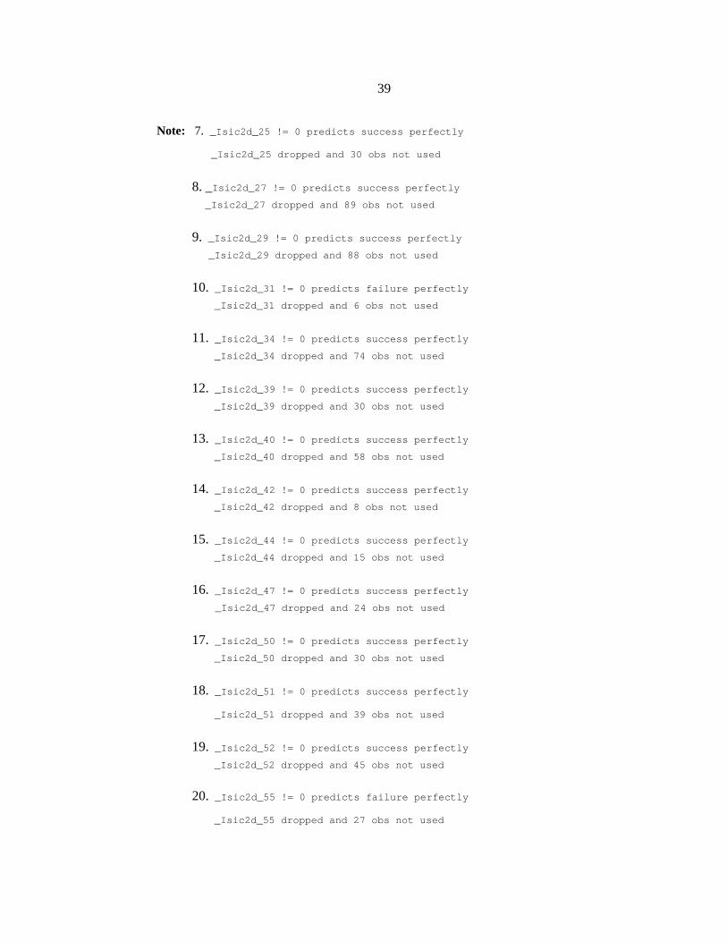
39
Note: 7. _Isic2d_25 != 0 predicts success perfectly _Isic2d_25 dropped and 30 obs not used
8. _Isic2d_27 != 0 predicts success perfectly _Isic2d_27 dropped and 89 obs not used
9. _Isic2d_29 != 0 predicts success perfectly _Isic2d_29 dropped and 88 obs not used
10. _Isic2d_31 != 0 predicts failure perfectly _Isic2d_31 dropped and 6 obs not used
11. _Isic2d_34 != 0 predicts success perfectly _Isic2d_34 dropped and 74 obs not used
12. _Isic2d_39 != 0 predicts success perfectly _Isic2d_39 dropped and 30 obs not used
13. _Isic2d_40 != 0 predicts success perfectly _Isic2d_40 dropped and 58 obs not used
14. _Isic2d_42 != 0 predicts success perfectly _Isic2d_42 dropped and 8 obs not used
15. _Isic2d_44 != 0 predicts success perfectly _Isic2d_44 dropped and 15 obs not used
16. _Isic2d_47 != 0 predicts success perfectly _Isic2d_47 dropped and 24 obs not used
17. _Isic2d_50 != 0 predicts success perfectly _Isic2d_50 dropped and 30 obs not used
18. _Isic2d_51 != 0 predicts success perfectly _Isic2d_51 dropped and 39 obs not used
19. _Isic2d_52 != 0 predicts success perfectly _Isic2d_52 dropped and 45 obs not used
20. _Isic2d_55 != 0 predicts failure perfectly
_Isic2d_55 dropped and 27 obs not used
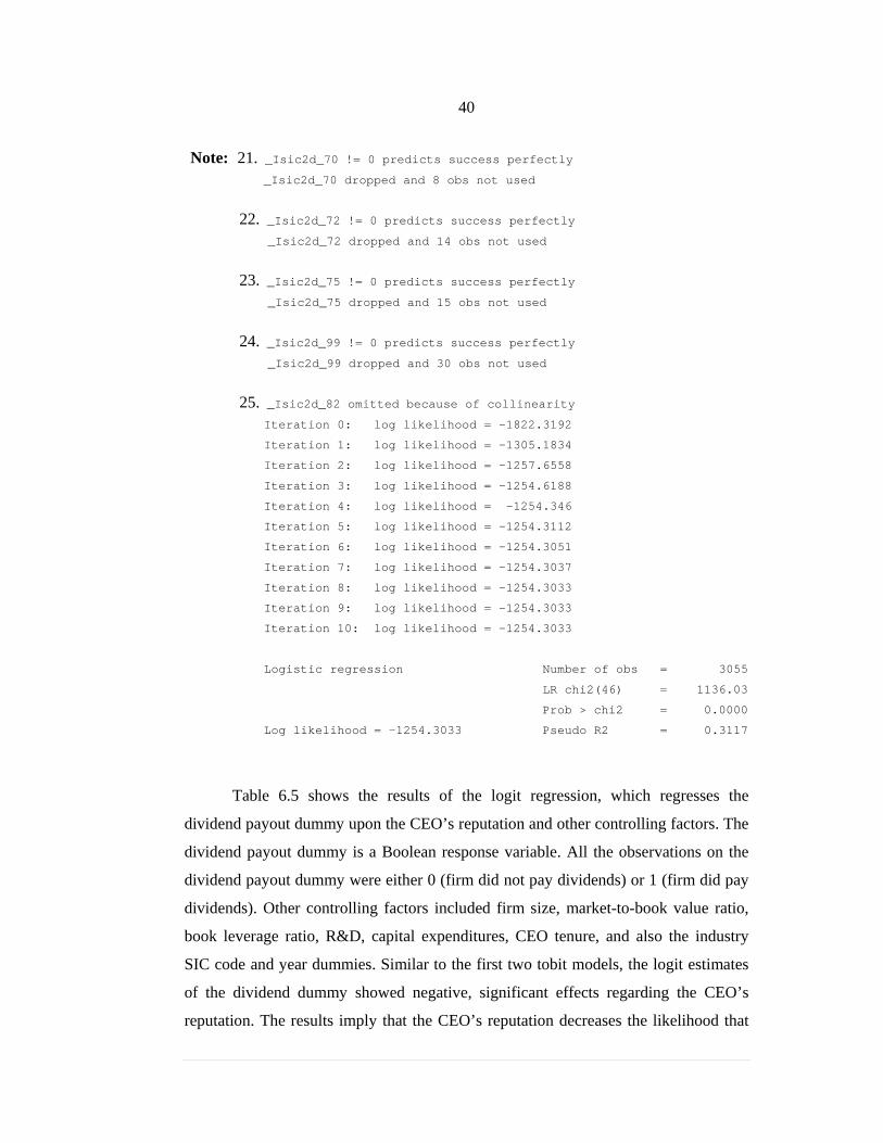
40
Note: 21. _Isic2d_70 != 0 predicts success perfectly _Isic2d_70 dropped and 8 obs not used
22. _Isic2d_72 != 0 predicts success perfectly _Isic2d_72 dropped and 14 obs not used
23. _Isic2d_75 != 0 predicts success perfectly _Isic2d_75 dropped and 15 obs not used
24. _Isic2d_99 != 0 predicts success perfectly _Isic2d_99 dropped and 30 obs not used
25. _Isic2d_82 omitted because of collinearity Iteration 0: log likelihood = -1822.3192
Iteration 1: log likelihood = -1305.1834
Iteration 2: log likelihood = -1257.6558
Iteration 3: log likelihood = -1254.6188
Iteration 4: log likelihood = -1254.346
Iteration 5: log likelihood = -1254.3112
Iteration 6: log likelihood = -1254.3051
Iteration 7: log likelihood = -1254.3037
Iteration 8: log likelihood = -1254.3033
Iteration 9: log likelihood = -1254.3033
Iteration 10: log likelihood = -1254.3033
Logistic regression Number of obs = 3055
LR chi2(46) = 1136.03
Prob > chi2 = 0.0000
Log likelihood = -1254.3033 Pseudo R2 = 0.3117
Table 6.5 shows the results of the logit regression, which regresses the
dividend payout dummy upon the CEO’s reputation and other controlling factors. The
dividend payout dummy is a Boolean response variable. All the observations on the
dividend payout dummy were either 0 (firm did not pay dividends) or 1 (firm did pay
dividends). Other controlling factors included firm size, market-to-book value ratio,
book leverage ratio, R&D, capital expenditures, CEO tenure, and also the industry
SIC code and year dummies. Similar to the first two tobit models, the logit estimates
of the dividend dummy showed negative, significant effects regarding the CEO’s
reputation. The results imply that the CEO’s reputation decreases the likelihood that
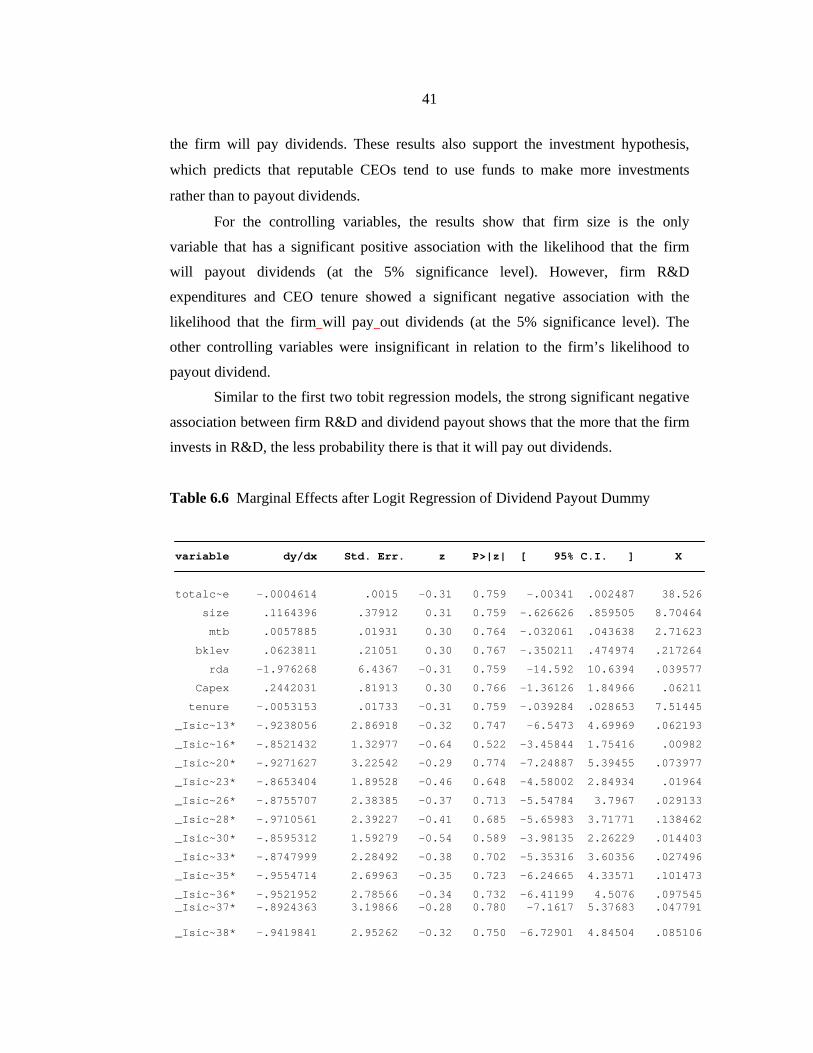
41
the firm will pay dividends. These results also support the investment hypothesis,
which predicts that reputable CEOs tend to use funds to make more investments
rather than to payout dividends.
For the controlling variables, the results show that firm size is the only
variable that has a significant positive association with the likelihood that the firm
will payout dividends (at the 5% significance level). However, firm R&D
expenditures and CEO tenure showed a significant negative association with the
likelihood that the firm will pay out dividends (at the 5% significance level). The
other controlling variables were insignificant in relation to the firm’s likelihood to
payout dividend.
Similar to the first two tobit regression models, the strong significant negative
association between firm R&D and dividend payout shows that the more that the firm
invests in R&D, the less probability there is that it will pay out dividends.
Table 6.6 Marginal Effects after Logit Regression of Dividend Payout Dummy
variable dy/dx Std. Err. z P>|z| [ 95% C.I. ] X
totalc~e -.0004614 .0015 -0.31 0.759 -.00341 .002487 38.526
size .1164396 .37912 0.31 0.759 -.626626 .859505 8.70464
mtb .0057885 .01931 0.30 0.764 -.032061 .043638 2.71623
bklev .0623811 .21051 0.30 0.767 -.350211 .474974 .217264
rda -1.976268 6.4367 -0.31 0.759 -14.592 10.6394 .039577
Capex .2442031 .81913 0.30 0.766 -1.36126 1.84966 .06211
tenure -.0053153 .01733 -0.31 0.759 -.039284 .028653 7.51445
_Isic~13* -.9238056 2.86918 -0.32 0.747 -6.5473 4.69969 .062193
_Isic~16* -.8521432 1.32977 -0.64 0.522 -3.45844 1.75416 .00982
_Isic~20* -.9271627 3.22542 -0.29 0.774 -7.24887 5.39455 .073977
_Isic~23* -.8653404 1.89528 -0.46 0.648 -4.58002 2.84934 .01964
_Isic~26* -.8755707 2.38385 -0.37 0.713 -5.54784 3.7967 .029133
_Isic~28* -.9710561 2.39227 -0.41 0.685 -5.65983 3.71771 .138462
_Isic~30* -.8595312 1.59279 -0.54 0.589 -3.98135 2.26229 .014403
_Isic~33* -.8747999 2.28492 -0.38 0.702 -5.35316 3.60356 .027496
_Isic~35* -.9554714 2.69963 -0.35 0.723 -6.24665 4.33571 .101473
_Isic~36* -.9521952 2.78566 -0.34 0.732 -6.41199 4.5076 .097545 _Isic~37* -.8924363 3.19866 -0.28 0.780 -7.1617 5.37683 .047791 _Isic~38* -.9419841 2.95262 -0.32 0.750 -6.72901 4.84504 .085106
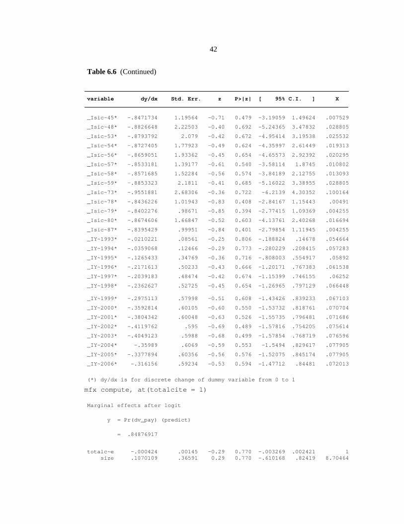
42
Table 6.6 (Continued)
variable dy/dx Std. Err. z P>|z| [ 95% C.I. ] X
_Isic~45* -.8471734 1.19564 -0.71 0.479 -3.19059 1.49624 .007529
_Isic~48* -.8826648 2.22503 -0.40 0.692 -5.24365 3.47832 .028805
_Isic~53* -.8793792 2.079 -0.42 0.672 -4.95414 3.19538 .025532
_Isic~54* -.8727405 1.77923 -0.49 0.624 -4.35997 2.61449 .019313
_Isic~56* -.8659051 1.93362 -0.45 0.654 -4.65573 2.92392 .020295
_Isic~57* -.8533181 1.39177 -0.61 0.540 -3.58114 1.8745 .010802
_Isic~58* -.8571685 1.52284 -0.56 0.574 -3.84189 2.12755 .013093
_Isic~59* -.8853323 2.1811 -0.41 0.685 -5.16022 3.38955 .028805
_Isic~73* -.9551881 2.68306 -0.36 0.722 -6.2139 4.30352 .100164
_Isic~78* -.8436226 1.01943 -0.83 0.408 -2.84167 1.15443 .00491
_Isic~79* -.8402276 .98671 -0.85 0.394 -2.77415 1.09369 .004255
_Isic~80* -.8674606 1.66847 -0.52 0.603 -4.13761 2.40268 .016694
_Isic~87* -.8395429 .99951 -0.84 0.401 -2.79854 1.11945 .004255
_IY~1993* -.0210221 .08561 -0.25 0.806 -.188824 .14678 .054664
_IY~1994* -.0359068 .12466 -0.29 0.773 -.280229 .208415 .057283
_IY~1995* -.1265433 .34769 -0.36 0.716 -.808003 .554917 .05892
_IY~1996* -.2171613 .50233 -0.43 0.666 -1.20171 .767383 .061538
_IY~1997* -.2039183 .48474 -0.42 0.674 -1.15399 .746155 .06252
_IY~1998* -.2362627 .52725 -0.45 0.654 -1.26965 .797129 .066448 _IY~1999* -.2975113 .57998 -0.51 0.608 -1.43426 .839233 .067103
_IY~2000* -.3592814 .60105 -0.60 0.550 -1.53732 .818761 .070704
_IY~2001* -.3804342 .60048 -0.63 0.526 -1.55735 .796481 .071686
_IY~2002* -.4119762 .595 -0.69 0.489 -1.57816 .754205 .075614
_IY~2003* -.4049123 .5988 -0.68 0.499 -1.57854 .768719 .076596
_IY~2004* -.35989 .6069 -0.59 0.553 -1.5494 .829617 .077905
_IY~2005* -.3377894 .60356 -0.56 0.576 -1.52075 .845174 .077905
_IY~2006* -.316156 .59234 -0.53 0.594 -1.47712 .84481 .072013
(*) dy/dx is for discrete change of dummy variable from 0 to 1
mfx compute, at(totalcite = 1)
Marginal effects after logit
y = Pr(dv_pay) (predict)
= .84876917
totalc~e -.000424 .00145 -0.29 0.770 -.003269 .002421 1 size .1070109 .36591 0.29 0.770 -.610168 .82419 8.70464
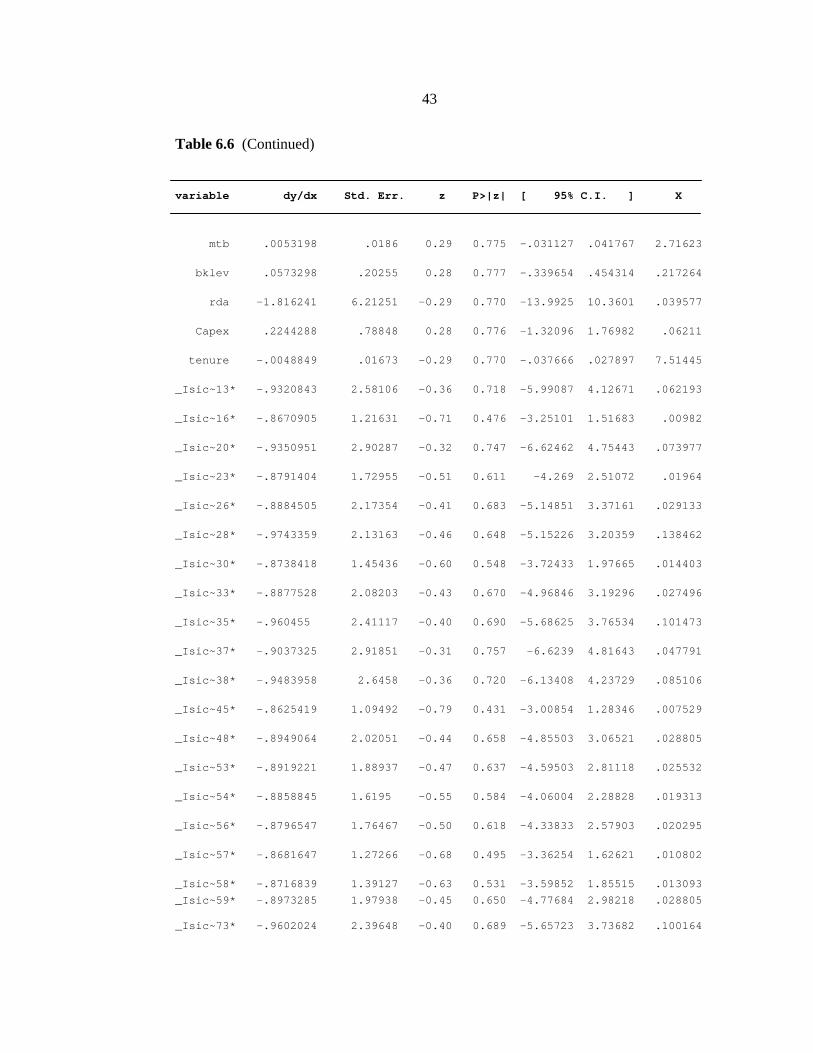
43
Table 6.6 (Continued)
variable dy/dx Std. Err. z P>|z| [ 95% C.I. ] X
mtb .0053198 .0186 0.29 0.775 -.031127 .041767 2.71623
bklev .0573298 .20255 0.28 0.777 -.339654 .454314 .217264
rda -1.816241 6.21251 -0.29 0.770 -13.9925 10.3601 .039577
Capex .2244288 .78848 0.28 0.776 -1.32096 1.76982 .06211
tenure -.0048849 .01673 -0.29 0.770 -.037666 .027897 7.51445
_Isic~13* -.9320843 2.58106 -0.36 0.718 -5.99087 4.12671 .062193
_Isic~16* -.8670905 1.21631 -0.71 0.476 -3.25101 1.51683 .00982
_Isic~20* -.9350951 2.90287 -0.32 0.747 -6.62462 4.75443 .073977
_Isic~23* -.8791404 1.72955 -0.51 0.611 -4.269 2.51072 .01964
_Isic~26* -.8884505 2.17354 -0.41 0.683 -5.14851 3.37161 .029133
_Isic~28* -.9743359 2.13163 -0.46 0.648 -5.15226 3.20359 .138462
_Isic~30* -.8738418 1.45436 -0.60 0.548 -3.72433 1.97665 .014403
_Isic~33* -.8877528 2.08203 -0.43 0.670 -4.96846 3.19296 .027496
_Isic~35* -.960455 2.41117 -0.40 0.690 -5.68625 3.76534 .101473
_Isic~37* -.9037325 2.91851 -0.31 0.757 -6.6239 4.81643 .047791
_Isic~38* -.9483958 2.6458 -0.36 0.720 -6.13408 4.23729 .085106
_Isic~45* -.8625419 1.09492 -0.79 0.431 -3.00854 1.28346 .007529
_Isic~48* -.8949064 2.02051 -0.44 0.658 -4.85503 3.06521 .028805
_Isic~53* -.8919221 1.88937 -0.47 0.637 -4.59503 2.81118 .025532
_Isic~54* -.8858845 1.6195 -0.55 0.584 -4.06004 2.28828 .019313
_Isic~56* -.8796547 1.76467 -0.50 0.618 -4.33833 2.57903 .020295
_Isic~57* -.8681647 1.27266 -0.68 0.495 -3.36254 1.62621 .010802
_Isic~58* -.8716839 1.39127 -0.63 0.531 -3.59852 1.85515 .013093
_Isic~59* -.8973285 1.97938 -0.45 0.650 -4.77684 2.98218 .028805 _Isic~73* -.9602024 2.39648 -0.40 0.689 -5.65723 3.73682 .100164
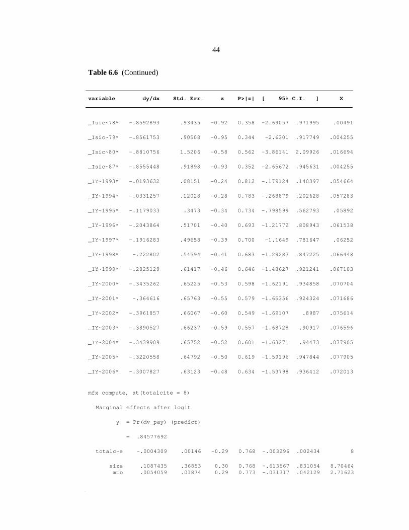
44
Table 6.6 (Continued)
variable dy/dx Std. Err. z P>|z| [ 95% C.I. ] X
_Isic~78* -.8592893 .93435 -0.92 0.358 -2.69057 .971995 .00491
_Isic~79* -.8561753 .90508 -0.95 0.344 -2.6301 .917749 .004255
_Isic~80* -.8810756 1.5206 -0.58 0.562 -3.86141 2.09926 .016694
_Isic~87* -.8555448 .91898 -0.93 0.352 -2.65672 .945631 .004255
_IY~1993* -.0193632 .08151 -0.24 0.812 -.179124 .140397 .054664
_IY~1994* -.0331257 .12028 -0.28 0.783 -.268879 .202628 .057283
_IY~1995* -.1179033 .3473 -0.34 0.734 -.798599 .562793 .05892
_IY~1996* -.2043864 .51701 -0.40 0.693 -1.21772 .808943 .061538
_IY~1997* -.1916283 .49658 -0.39 0.700 -1.1649 .781647 .06252
_IY~1998* -.222802 .54594 -0.41 0.683 -1.29283 .847225 .066448
_IY~1999* -.2825129 .61417 -0.46 0.646 -1.48627 .921241 .067103
_IY~2000* -.3435262 .65225 -0.53 0.598 -1.62191 .934858 .070704
_IY~2001* -.364616 .65763 -0.55 0.579 -1.65356 .924324 .071686
_IY~2002* -.3961857 .66067 -0.60 0.549 -1.69107 .8987 .075614
_IY~2003* -.3890527 .66237 -0.59 0.557 -1.68728 .90917 .076596
_IY~2004* -.3439909 .65752 -0.52 0.601 -1.63271 .94473 .077905
_IY~2005* -.3220558 .64792 -0.50 0.619 -1.59196 .947844 .077905
_IY~2006* -.3007827 .63123 -0.48 0.634 -1.53798 .936412 .072013
mfx compute, at(totalcite = 8)
Marginal effects after logit
y = Pr(dv_pay) (predict)
= .84577692
totalc~e -.0004309 .00146 -0.29 0.768 -.003296 .002434 8
size .1087435 .36853 0.30 0.768 -.613567 .831054 8.70464 mtb .0054059 .01874 0.29 0.773 -.031317 .042129 2.71623
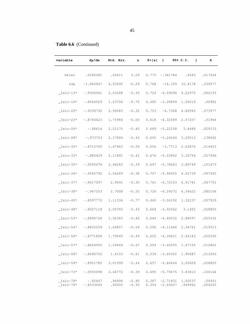
45
Table 6.6 (Continued)
variable dy/dx Std. Err. z P>|z| [ 95% C.I. ] X
bklev .0582581 .20411 0.29 0.775 -.341784 .4583 .217264
rda -1.845647 6.25695 -0.29 0.768 -14.109 10.4178 .039577
_Isic~13* -.9306061 2.63288 -0.35 0.724 -6.09096 4.22975 .062193
_Isic~16* -.8644029 1.23706 -0.70 0.485 -3.28899 1.56019 .00982
_Isic~20* -.9336792 2.96083 -0.32 0.753 -6.7368 4.86945 .073977
_Isic~23* -.8766623 1.75984 -0.50 0.618 -4.32589 2.57257 .01964
_Isic~26* -.88614 2.21175 -0.40 0.689 -5.22108 3.4488 .029133
_Isic~28* -.973753 2.17804 -0.45 0.655 -5.24264 3.29513 .138462
_Isic~30* -.8712705 1.47963 -0.59 0.556 -3.7713 2.02876 .014403
_Isic~33* -.885429 2.11891 -0.42 0.676 -5.03842 3.26756 .027496
_Isic~35* -.9595678 2.46283 -0.39 0.697 -5.78663 3.86749 .101473
_Isic~36* -.9565792 2.54289 -0.38 0.707 -5.94055 4.02739 .097545
_Isic~37* -.9017097 2.9691 -0.30 0.761 -6.72103 4.91761 .047791
_Isic~38* -.947253 2.7008 -0.35 0.726 -6.24072 4.34622 .085106
_Isic~45* -.8597772 1.11336 -0.77 0.440 -3.04192 1.32237 .007529
_Isic~48* -.8927118 2.05765 -0.43 0.664 -4.92562 3.1402 .028805
_Isic~53* -.8896728 1.92383 -0.46 0.644 -4.66032 2.88097 .025532
_Isic~54* -.8835259 1.64857 -0.54 0.592 -4.11466 2.34761 .019313
_Isic~56* -.8771858 1.79545 -0.49 0.625 -4.39621 2.64183 .020295
_Isic~57* -.8654955 1.29444 -0.67 0.504 -3.40255 1.67155 .010802
_Isic~58* -.8690752 1.4153 -0.61 0.539 -3.64302 1.90487 .013093
_Isic~59* -.8951785 2.01599 -0.44 0.657 -4.84644 3.05609 .028805
_Isic~73* -.9593098 2.44772 -0.39 0.695 -5.75675 3.83813 .100164
_Isic~78* -.85647 .94994 -0.90 0.367 -2.71831 1.00537 .00491 _Isic~79* -.8533045 .92005 -0.93 0.354 -2.65657 .949962 .004255
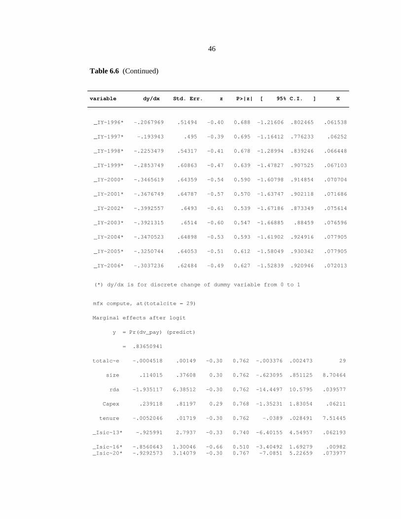
46
Table 6.6 (Continued)
variable dy/dx Std. Err. z P>|z| [ 95% C.I. ] X
_IY~1996* -.2067969 .51494 -0.40 0.688 -1.21606 .802465 .061538
_IY~1997* -.193943 .495 -0.39 0.695 -1.16412 .776233 .06252
_IY~1998* -.2253479 .54317 -0.41 0.678 -1.28994 .839246 .066448
_IY~1999* -.2853749 .60863 -0.47 0.639 -1.47827 .907525 .067103
_IY~2000* -.3465619 .64359 -0.54 0.590 -1.60798 .914854 .070704
_IY~2001* -.3676749 .64787 -0.57 0.570 -1.63747 .902118 .071686
_IY~2002* -.3992557 .6493 -0.61 0.539 -1.67186 .873349 .075614
_IY~2003* -.3921315 .6514 -0.60 0.547 -1.66885 .88459 .076596
_IY~2004* -.3470523 .64898 -0.53 0.593 -1.61902 .924916 .077905
_IY~2005* -.3250744 .64053 -0.51 0.612 -1.58049 .930342 .077905
_IY~2006* -.3037236 .62484 -0.49 0.627 -1.52839 .920946 .072013 (*) dy/dx is for discrete change of dummy variable from 0 to 1
mfx compute, at(totalcite = 29)
Marginal effects after logit
y = Pr(dv_pay) (predict)
= .83650941
totalc~e -.0004518 .00149 -0.30 0.762 -.003376 .002473 29
size .114015 .37608 0.30 0.762 -.623095 .851125 8.70464
rda -1.935117 6.38512 -0.30 0.762 -14.4497 10.5795 .039577
Capex .239118 .81197 0.29 0.768 -1.35231 1.83054 .06211
tenure -.0052046 .01719 -0.30 0.762 -.0389 .028491 7.51445
_Isic~13* -.925991 2.7937 -0.33 0.740 -6.40155 4.54957 .062193
_Isic~16* -.8560643 1.30046 -0.66 0.510 -3.40492 1.69279 .00982 _Isic~20* -.9292573 3.14079 -0.30 0.767 -7.0851 5.22659 .073977

47
Table 6.6 (Continued)
variable dy/dx Std. Err. z P>|z| [ 95% C.I. ] X
_Isic~23* -.8689648 1.85238 -0.47 0.639 -4.49956 2.76163 .01964
_Isic~26* -.8789565 2.3292 -0.38 0.706 -5.44411 3.6862 .029133
_Isic~28* -.9719255 2.32334 -0.42 0.676 -5.52558 3.58173 .138462
_Isic~30* -.8632877 1.55697 -0.55 0.579 -3.9149 2.18832 .014403
_Isic~33* -.8782046 2.23223 -0.39 0.694 -5.25329 3.49688 .027496
_Isic~35* -.9567905 2.6236 -0.36 0.715 -6.09894 4.18536 .101473
_Isic~36* -.9536066 2.70766 -0.35 0.725 -6.26053 4.35332 .097545
_Isic~37* -.8954106 3.12545 -0.29 0.775 -7.02118 5.23036 .047791
_Isic~38* -.9436793 2.87191 -0.33 0.742 -6.57252 4.68516 .085106
_Isic~53* -.8826774 2.02973 -0.43 0.664 -4.86088 3.09553 .025532
_Isic~54* -.8761947 1.73779 -0.50 0.614 -4.2822 2.52981 .019313
_Isic~56* -.8695164 1.88985 -0.46 0.645 -4.57354 2.83451 .020295
_Isic~57* -.8572132 1.36099 -0.63 0.529 -3.52471 1.81029 .010802
_Isic~58* -.860978 1.48881 -0.58 0.563 -3.779 2.05704 .013093
_Isic~59* -.8884884 2.12863 -0.42 0.676 -5.06053 3.28355 .028805
_Isic~73* -.9565153 2.6075 -0.37 0.714 -6.06712 4.15409 .100164
_Isic~80* -.871037 1.63017 -0.53 0.593 -4.06611 2.32403 .016694
_Isic~87* -.8437361 .97874 -0.86 0.389 -2.76204 1.07457 .004255
_IY~1993* -.0205965 .08461 -0.24 0.808 -.186438 .145245 .054664
_IY~1994* -.0351943 .12365 -0.28 0.776 -.277535 .207146 .057283
_IY~1995* -.1243518 .34807 -0.36 0.721 -.806561 .557858 .05892
_IY~1996* -.2139567 .5069 -0.42 0.673 -1.20745 .779541 .061538
_IY~1997* -.2008299 .48854 -0.41 0.681 -1.15835 .756689 .06252
_IY~1998* -.2328936 .5329 -0.44 0.662 -1.27735 .811564 .066448 _IY~1999* -.2937892 .58971 -0.50 0.618 -1.44959 .862016 .067103
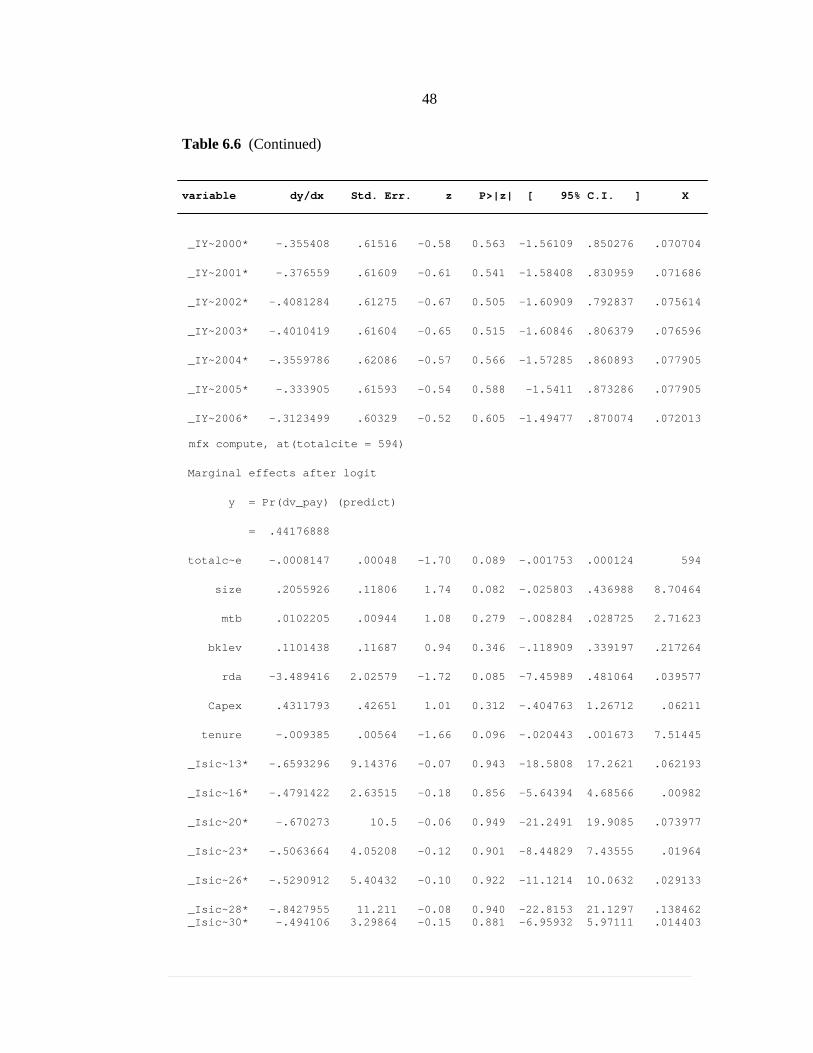
48
Table 6.6 (Continued)
variable dy/dx Std. Err. z P>|z| [ 95% C.I. ] X
_IY~2000* -.355408 .61516 -0.58 0.563 -1.56109 .850276 .070704
_IY~2001* -.376559 .61609 -0.61 0.541 -1.58408 .830959 .071686
_IY~2002* -.4081284 .61275 -0.67 0.505 -1.60909 .792837 .075614
_IY~2003* -.4010419 .61604 -0.65 0.515 -1.60846 .806379 .076596
_IY~2004* -.3559786 .62086 -0.57 0.566 -1.57285 .860893 .077905
_IY~2005* -.333905 .61593 -0.54 0.588 -1.5411 .873286 .077905
_IY~2006* -.3123499 .60329 -0.52 0.605 -1.49477 .870074 .072013 mfx compute, at(totalcite = 594)
Marginal effects after logit
y = Pr(dv_pay) (predict)
= .44176888
totalc~e -.0008147 .00048 -1.70 0.089 -.001753 .000124 594
size .2055926 .11806 1.74 0.082 -.025803 .436988 8.70464
mtb .0102205 .00944 1.08 0.279 -.008284 .028725 2.71623
bklev .1101438 .11687 0.94 0.346 -.118909 .339197 .217264
rda -3.489416 2.02579 -1.72 0.085 -7.45989 .481064 .039577
Capex .4311793 .42651 1.01 0.312 -.404763 1.26712 .06211
tenure -.009385 .00564 -1.66 0.096 -.020443 .001673 7.51445
_Isic~13* -.6593296 9.14376 -0.07 0.943 -18.5808 17.2621 .062193
_Isic~16* -.4791422 2.63515 -0.18 0.856 -5.64394 4.68566 .00982
_Isic~20* -.670273 10.5 -0.06 0.949 -21.2491 19.9085 .073977
_Isic~23* -.5063664 4.05208 -0.12 0.901 -8.44829 7.43555 .01964
_Isic~26* -.5290912 5.40432 -0.10 0.922 -11.1214 10.0632 .029133
_Isic~28* -.8427955 11.211 -0.08 0.940 -22.8153 21.1297 .138462 _Isic~30* -.494106 3.29864 -0.15 0.881 -6.95932 5.97111 .014403

49
Table 6.6 (Continued)
variable dy/dx Std. Err. z P>|z| [ 95% C.I. ] X
_Isic~33* -.5272995 5.17035 -0.10 0.919 -10.661 9.60639 .027496
_Isic~35* -.7740517 11.075 -0.07 0.944 -22.4805 20.9324 .101473
_Isic~36* -.7607714 11.113 -0.07 0.945 -22.542 21.0204 .097545
_Isic~37* -.5701622 7.95916 -0.07 0.943 -16.1698 15.0295 .047791
_Isic~38* -.7216223 10.828 -0.07 0.947 -21.9434 20.5002 .085106
_Isic~45* -.4694423 2.30149 -0.20 0.838 -4.98028 4.0414 .007529
_Isic~48* -.5456094 5.32708 -0.10 0.918 -10.9865 9.89527 .028805
_Isic~53* -.5378234 4.87264 -0.11 0.912 -10.088 9.01237 .025532
_Isic~54* -.5225879 3.99748 -0.13 0.896 -8.3575 7.31232 .019313
_Isic~56* -.5075848 4.14598 -0.12 0.903 -8.63355 7.61838 .020295
_Isic~57* -.4814791 2.77721 -0.17 0.862 -5.92471 4.96175 .010802
_Isic~58* -.4892492 3.10926 -0.16 0.875 -6.58329 5.60479 .013093
_Isic~59* -.5520458 5.31357 -0.10 0.917 -10.9665 9.86237 .028805
_Isic~73* -.7728827 10.983 -0.07 0.944 -22.2993 20.7536 .100164
_Isic~78* -.4626783 1.92272 -0.24 0.810 -4.23114 3.30578 .00491
_Isic~79* -.4563507 1.82532 -0.25 0.803 -4.03392 3.12122 .004255
_Isic~80* -.5109217 3.62709 -0.14 0.888 -7.61988 6.59804 .016694
_Isic~87* -.4551068 1.8245 -0.25 0.803 -4.03106 3.12085 .004255
_IY~1993* -.0352682 .08971 -0.39 0.694 -.211092 .140555 .054664
_IY~1994* -.0582085 .09648 -0.60 0.546 -.247296 .130879 .057283
_IY~1995* -.1699847 .23177 -0.73 0.463 -.62425 .284281 .05892
_IY~1996* -.2495289 .40899 -0.61 0.542 -1.05113 .55207 .061538
_IY~1997* -.239563 .38311 -0.63 0.532 -.990452 .511326 .06252
_IY~1998* -.2644329 .44468 -0.59 0.552 -1.13598 .607115 .066448 _IY~1999* -.3045458 .55669 -0.55 0.584 -1.39564 .786552 .067103
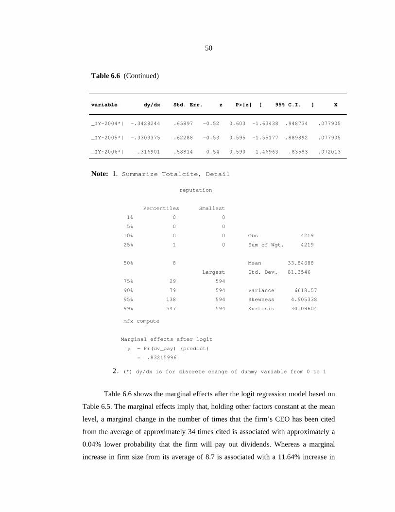
50
Table 6.6 (Continued)
variable dy/dx Std. Err. z P>|z| [ 95% C.I. ] X _IY~2004*| -.3428244 .65897 -0.52 0.603 -1.63438 .948734 .077905
_IY~2005*| -.3309375 .62288 -0.53 0.595 -1.55177 .889892 .077905
_IY~2006*| -.316901 .58814 -0.54 0.590 -1.46963 .83583 .072013
Note: 1. Summarize Totalcite, Detail
reputation
Percentiles Smallest
1% 0 0
5% 0 0
10% 0 0 Obs 4219
25% 1 0 Sum of Wgt. 4219
50% 8 Mean 33.84688
Largest Std. Dev. 81.3546
75% 29 594
90% 79 594 Variance 6618.57
95% 138 594 Skewness 4.905338
99% 547 594 Kurtosis 30.09604 mfx compute
Marginal effects after logit
y = Pr(dv_pay) (predict)
= .83215996
2. (*) dy/dx is for discrete change of dummy variable from 0 to 1
Table 6.6 shows the marginal effects after the logit regression model based on
Table 6.5. The marginal effects imply that, holding other factors constant at the mean
level, a marginal change in the number of times that the firm’s CEO has been cited
from the average of approximately 34 times cited is associated with approximately a
0.04% lower probability that the firm will pay out dividends. Whereas a marginal
increase in firm size from its average of 8.7 is associated with a 11.64% increase in
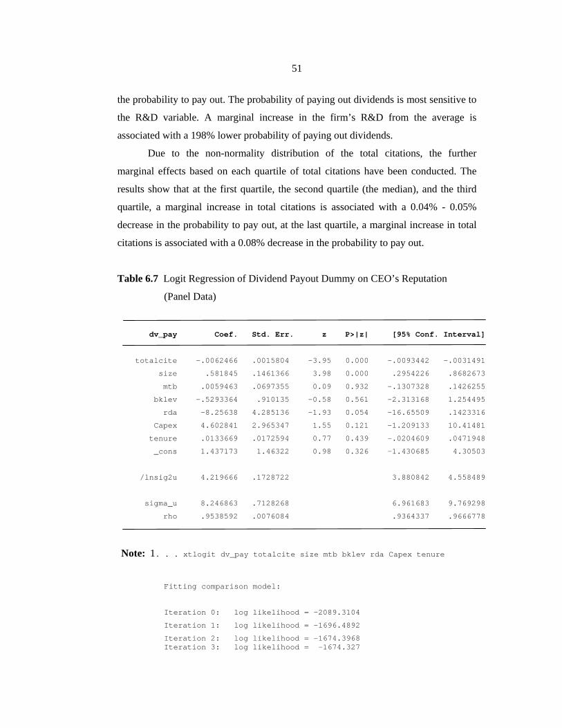
51
the probability to pay out. The probability of paying out dividends is most sensitive to
the R&D variable. A marginal increase in the firm’s R&D from the average is
associated with a 198% lower probability of paying out dividends.
Due to the non-normality distribution of the total citations, the further
marginal effects based on each quartile of total citations have been conducted. The
results show that at the first quartile, the second quartile (the median), and the third
quartile, a marginal increase in total citations is associated with a 0.04% - 0.05%
decrease in the probability to pay out, at the last quartile, a marginal increase in total
citations is associated with a 0.08% decrease in the probability to pay out.
Table 6.7 Logit Regression of Dividend Payout Dummy on CEO’s Reputation
(Panel Data)
dv_pay Coef. Std. Err. z P>|z| [95% Conf. Interval]
totalcite -.0062466 .0015804 -3.95 0.000 -.0093442 -.0031491
size .581845 .1461366 3.98 0.000 .2954226 .8682673
mtb .0059463 .0697355 0.09 0.932 -.1307328 .1426255
bklev -.5293364 .910135 -0.58 0.561 -2.313168 1.254495
rda -8.25638 4.285136 -1.93 0.054 -16.65509 .1423316
Capex 4.602841 2.965347 1.55 0.121 -1.209133 10.41481
tenure .0133669 .0172594 0.77 0.439 -.0204609 .0471948
_cons 1.437173 1.46322 0.98 0.326 -1.430685 4.30503
/lnsig2u 4.219666 .1728722 3.880842 4.558489
sigma_u 8.246863 .7128268 6.961683 9.769298
rho .9538592 .0076084 .9364337 .9666778
Note: 1. . . xtlogit dv_pay totalcite size mtb bklev rda Capex tenure
Fitting comparison model:
Iteration 0: log likelihood = -2089.3104
Iteration 1: log likelihood = -1696.4892
Iteration 2: log likelihood = -1674.3968 Iteration 3: log likelihood = -1674.327
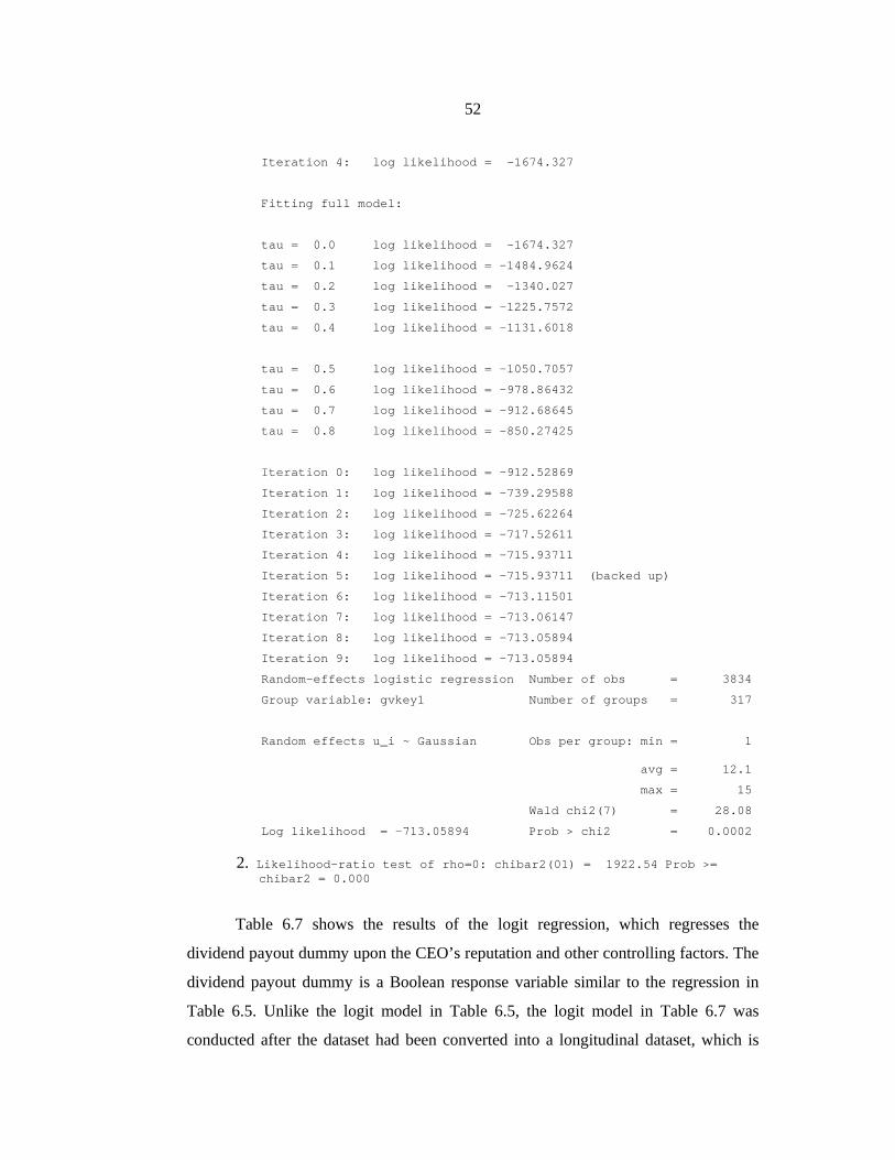
52
Iteration 4: log likelihood = -1674.327
Fitting full model:
tau = 0.0 log likelihood = -1674.327
tau = 0.1 log likelihood = -1484.9624
tau = 0.2 log likelihood = -1340.027
tau = 0.3 log likelihood = -1225.7572
tau = 0.4 log likelihood = -1131.6018
tau = 0.5 log likelihood = -1050.7057
tau = 0.6 log likelihood = -978.86432
tau = 0.7 log likelihood = -912.68645
tau = 0.8 log likelihood = -850.27425
Iteration 0: log likelihood = -912.52869
Iteration 1: log likelihood = -739.29588
Iteration 2: log likelihood = -725.62264
Iteration 3: log likelihood = -717.52611
Iteration 4: log likelihood = -715.93711
Iteration 5: log likelihood = -715.93711 (backed up)
Iteration 6: log likelihood = -713.11501
Iteration 7: log likelihood = -713.06147
Iteration 8: log likelihood = -713.05894
Iteration 9: log likelihood = -713.05894
Random-effects logistic regression Number of obs = 3834
Group variable: gvkey1 Number of groups = 317
Random effects u_i ~ Gaussian Obs per group: min = 1 avg = 12.1
max = 15
Wald chi2(7) = 28.08
Log likelihood = -713.05894 Prob > chi2 = 0.0002
2. Likelihood-ratio test of rho=0: chibar2(01) = 1922.54 Prob >= chibar2 = 0.000
Table 6.7 shows the results of the logit regression, which regresses the
dividend payout dummy upon the CEO’s reputation and other controlling factors. The
dividend payout dummy is a Boolean response variable similar to the regression in
Table 6.5. Unlike the logit model in Table 6.5, the logit model in Table 6.7 was
conducted after the dataset had been converted into a longitudinal dataset, which is
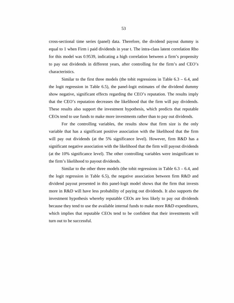
53
cross-sectional time series (panel) data. Therefore, the dividend payout dummy is
equal to 1 when Firm i paid dividends in year t. The intra-class latent correlation Rho
for this model was 0.9539, indicating a high correlation between a firm’s propensity
to pay out dividends in different years, after controlling for the firm’s and CEO’s
characteristics.
Similar to the first three models (the tobit regressions in Table 6.3 – 6.4, and
the logit regression in Table 6.5), the panel-logit estimates of the dividend dummy
show negative, significant effects regarding the CEO’s reputation. The results imply
that the CEO’s reputation decreases the likelihood that the firm will pay dividends.
These results also support the investment hypothesis, which predicts that reputable
CEOs tend to use funds to make more investments rather than to pay out dividends.
For the controlling variables, the results show that firm size is the only
variable that has a significant positive association with the likelihood that the firm
will pay out dividends (at the 5% significance level). However, firm R&D has a
significant negative association with the likelihood that the firm will payout dividends
(at the 10% significance level). The other controlling variables were insignificant to
the firm’s likelihood to payout dividends.
Similar to the other three models (the tobit regressions in Table 6.3 – 6.4, and
the logit regression in Table 6.5), the negative association between firm R&D and
dividend payout presented in this panel-logit model shows that the firm that invests
more in R&D will have less probability of paying out dividends. It also supports the
investment hypothesis whereby reputable CEOs are less likely to pay out dividends
because they tend to use the available internal funds to make more R&D expenditures,
which implies that reputable CEOs tend to be confident that their investments will
turn out to be successful.
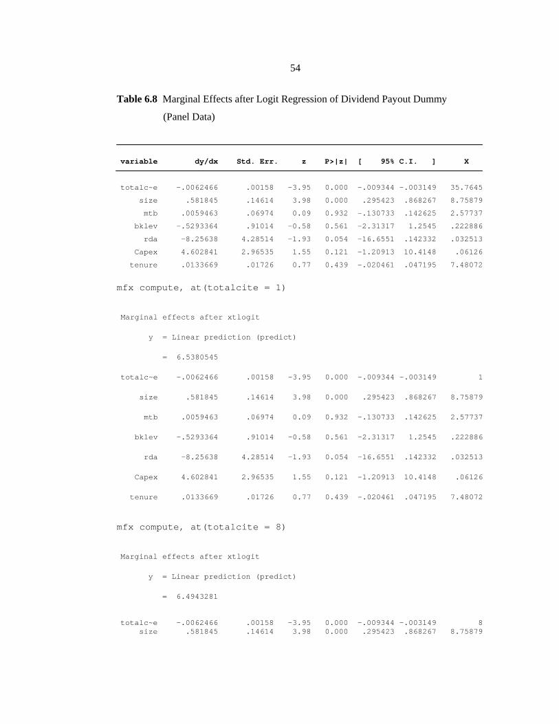
54
Table 6.8 Marginal Effects after Logit Regression of Dividend Payout Dummy
(Panel Data)
variable dy/dx Std. Err. z P>|z| [ 95% C.I. ] X
totalc~e -.0062466 .00158 -3.95 0.000 -.009344 -.003149 35.7645
size .581845 .14614 3.98 0.000 .295423 .868267 8.75879
mtb .0059463 .06974 0.09 0.932 -.130733 .142625 2.57737
bklev -.5293364 .91014 -0.58 0.561 -2.31317 1.2545 .222886
rda -8.25638 4.28514 -1.93 0.054 -16.6551 .142332 .032513
Capex 4.602841 2.96535 1.55 0.121 -1.20913 10.4148 .06126
tenure .0133669 .01726 0.77 0.439 -.020461 .047195 7.48072
mfx compute, at(totalcite = 1)
Marginal effects after xtlogit
y = Linear prediction (predict)
= 6.5380545
totalc~e -.0062466 .00158 -3.95 0.000 -.009344 -.003149 1
size .581845 .14614 3.98 0.000 .295423 .868267 8.75879
mtb .0059463 .06974 0.09 0.932 -.130733 .142625 2.57737
bklev -.5293364 .91014 -0.58 0.561 -2.31317 1.2545 .222886
rda -8.25638 4.28514 -1.93 0.054 -16.6551 .142332 .032513
Capex 4.602841 2.96535 1.55 0.121 -1.20913 10.4148 .06126
tenure .0133669 .01726 0.77 0.439 -.020461 .047195 7.48072
mfx compute, at(totalcite = 8)
Marginal effects after xtlogit
y = Linear prediction (predict)
= 6.4943281 totalc~e -.0062466 .00158 -3.95 0.000 -.009344 -.003149 8 size .581845 .14614 3.98 0.000 .295423 .868267 8.75879
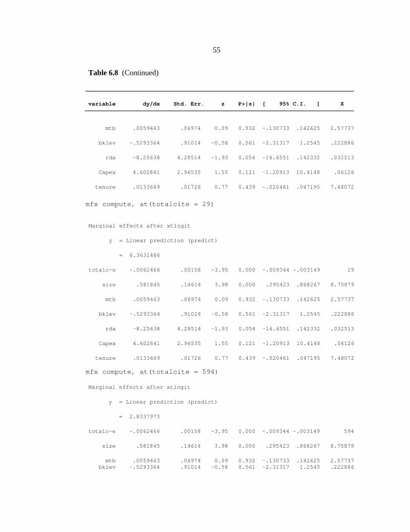
55
Table 6.8 (Continued)
variable dy/dx Std. Err. z P>|z| [ 95% C.I. ] X
mtb .0059463 .06974 0.09 0.932 -.130733 .142625 2.57737
bklev -.5293364 .91014 -0.58 0.561 -2.31317 1.2545 .222886
rda -8.25638 4.28514 -1.93 0.054 -16.6551 .142332 .032513
Capex 4.602841 2.96535 1.55 0.121 -1.20913 10.4148 .06126
tenure .0133669 .01726 0.77 0.439 -.020461 .047195 7.48072
mfx compute, at(totalcite = 29)
Marginal effects after xtlogit
y = Linear prediction (predict)
= 6.3631486
totalc~e -.0062466 .00158 -3.95 0.000 -.009344 -.003149 29
size .581845 .14614 3.98 0.000 .295423 .868267 8.75879
mtb .0059463 .06974 0.09 0.932 -.130733 .142625 2.57737
bklev -.5293364 .91014 -0.58 0.561 -2.31317 1.2545 .222886
rda -8.25638 4.28514 -1.93 0.054 -16.6551 .142332 .032513
Capex 4.602841 2.96535 1.55 0.121 -1.20913 10.4148 .06126
tenure .0133669 .01726 0.77 0.439 -.020461 .047195 7.48072 mfx compute, at(totalcite = 594)
Marginal effects after xtlogit
y = Linear prediction (predict)
= 2.8337973
totalc~e -.0062466 .00158 -3.95 0.000 -.009344 -.003149 594
size .581845 .14614 3.98 0.000 .295423 .868267 8.75879
mtb .0059463 .06974 0.09 0.932 -.130733 .142625 2.57737 bklev -.5293364 .91014 -0.58 0.561 -2.31317 1.2545 .222886
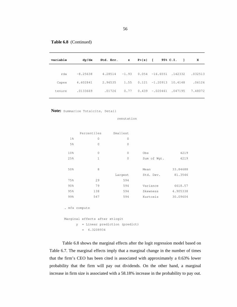
56
Table 6.8 (Continued)
variable dy/dx Std. Err. z P>|z| [ 95% C.I. ] X
rda -8.25638 4.28514 -1.93 0.054 -16.6551 .142332 .032513
Capex 4.602841 2.96535 1.55 0.121 -1.20913 10.4148 .06126
tenure .0133669 .01726 0.77 0.439 -.020461 .047195 7.48072
Note: Summarize Totalcite, Detail reputation
-------------------------------------------------------------
Percentiles Smallest
1% 0 0
5% 0 0
10% 0 0 Obs 4219
25% 1 0 Sum of Wgt. 4219
50% 8 Mean 33.84688
Largest Std. Dev. 81.3546
75% 29 594
90% 79 594 Variance 6618.57
95% 138 594 Skewness 4.905338
99% 547 594 Kurtosis 30.09604 . mfx compute
Marginal effects after xtlogit
y = Linear prediction (predict)
= 6.3208934
Table 6.8 shows the marginal effects after the logit regression model based on
Table 6.7. The marginal effects imply that a marginal change in the number of times
that the firm’s CEO has been cited is associated with approximately a 0.63% lower
probability that the firm will pay out dividends. On the other hand, a marginal
increase in firm size is associated with a 58.18% increase in the probability to pay out.
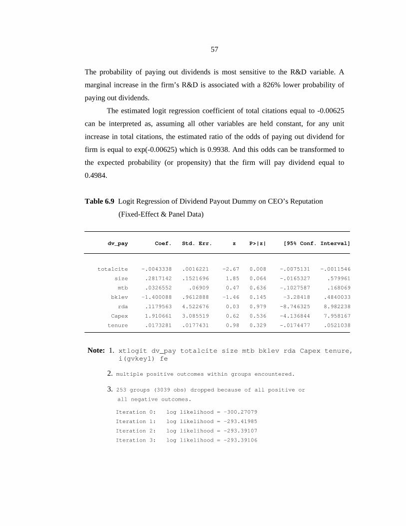
57
The probability of paying out dividends is most sensitive to the R&D variable. A
marginal increase in the firm’s R&D is associated with a 826% lower probability of
paying out dividends.
The estimated logit regression coefficient of total citations equal to -0.00625
can be interpreted as, assuming all other variables are held constant, for any unit
increase in total citations, the estimated ratio of the odds of paying out dividend for
firm is equal to exp(-0.00625) which is 0.9938. And this odds can be transformed to
the expected probability (or propensity) that the firm will pay dividend equal to
0.4984.
Table 6.9 Logit Regression of Dividend Payout Dummy on CEO’s Reputation
(Fixed-Effect & Panel Data)
dv_pay Coef. Std. Err. z P>|z| [95% Conf. Interval] totalcite -.0043338 .0016221 -2.67 0.008 -.0075131 -.0011546
size .2817142 .1521696 1.85 0.064 -.0165327 .579961
mtb .0326552 .06909 0.47 0.636 -.1027587 .168069
bklev -1.400088 .9612888 -1.46 0.145 -3.28418 .4840033
rda .1179563 4.522676 0.03 0.979 -8.746325 8.982238
Capex 1.910661 3.085519 0.62 0.536 -4.136844 7.958167
tenure .0173281 .0177431 0.98 0.329 -.0174477 .0521038
Note: 1. xtlogit dv_pay totalcite size mtb bklev rda Capex tenure, i(gvkey1) fe
2. multiple positive outcomes within groups encountered.
3. 253 groups (3039 obs) dropped because of all positive or all negative outcomes.
Iteration 0: log likelihood = -300.27079
Iteration 1: log likelihood = -293.41985
Iteration 2: log likelihood = -293.39107
Iteration 3: log likelihood = -293.39106
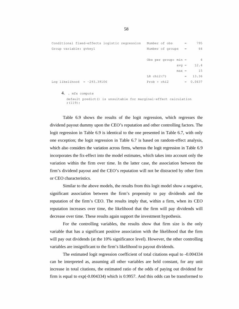
58
Conditional fixed-effects logistic regression Number of obs = 795
Group variable: gvkey1 Number of groups = 64
Obs per group: min = 4
avg = 12.4
max = 15
LR chi2(7) = 13.36
Log likelihood = -293.39106 Prob > chi2 = 0.0637
4. . mfx compute
default predict() is unsuitable for marginal-effect calculation r(119);
Table 6.9 shows the results of the logit regression, which regresses the
dividend payout dummy upon the CEO’s reputation and other controlling factors. The
logit regression in Table 6.9 is identical to the one presented in Table 6.7, with only
one exception; the logit regression in Table 6.7 is based on random-effect analysis,
which also considers the variation across firms, whereas the logit regression in Table 6.9
incorporates the fix-effect into the model estimates, which takes into account only the
variation within the firm over time. In the latter case, the association between the
firm’s dividend payout and the CEO’s reputation will not be distracted by other firm
or CEO characteristics.
Similar to the above models, the results from this logit model show a negative,
significant association between the firm’s propensity to pay dividends and the
reputation of the firm’s CEO. The results imply that, within a firm, when its CEO
reputation increases over time, the likelihood that the firm will pay dividends will
decrease over time. These results again support the investment hypothesis.
For the controlling variables, the results show that firm size is the only
variable that has a significant positive association with the likelihood that the firm
will pay out dividends (at the 10% significance level). However, the other controlling
variables are insignificant to the firm’s likelihood to payout dividends.
The estimated logit regression coefficient of total citations equal to -0.004334
can be interpreted as, assuming all other variables are held constant, for any unit
increase in total citations, the estimated ratio of the odds of paying out dividend for
firm is equal to exp(-0.004334) which is 0.9957. And this odds can be transformed to
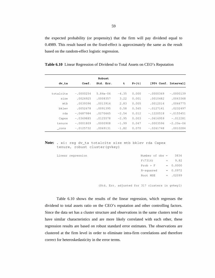
59
the expected probability (or propensity) that the firm will pay dividend equal to
0.4989. This result based on the fixed-effect is approximately the same as the result
based on the random-effect logistic regression.
Table 6.10 Linear Regression of Dividend to Total Assets on CEO’s Reputation
Robust
dv_ta Coef. Std. Err. t P>|t| [95% Conf. Interval] totalcite -.0000254 5.84e-06 -4.35 0.000 -.0000369 -.0000139
size .0026925 .0008357 3.22 0.001 .0010482 .0043368
mtb .0039396 .0013916 2.83 0.005 .0012016 .0066775
bklev .0052678 .0091395 0.58 0.565 -.0127141 .0232497
rda -.0687984 .0270665 -2.54 0.012 -.1220518 -.0155451
Capex -.0369885 .0125578 -2.95 0.003 -.0616959 -.012281
tenure -.0001809 .0000908 -1.99 0.047 -.0003596 -2.20e-06
_cons -.0125732 .0069131 -1.82 0.070 -.0261748 .0010284
Note: . xi: reg dv_ta totalcite size mtb bklev rda Capex tenure, robust cluster(gvkey)
Linear regression Number of obs = 3834
F(7316) = 9.82
Prob > F = 0.0000
R-squared = 0.0972
Root MSE = .02099 (Std. Err. adjusted for 317 clusters in gvkey1)
Table 6.10 shows the results of the linear regression, which regresses the
dividend to total assets ratio on the CEO’s reputation and other controlling factors.
Since the data set has a cluster structure and observations in the same clusters tend to
have similar characteristics and are more likely correlated with each other, these
regression results are based on robust standard error estimates. The observations are
clustered at the firm level in order to eliminate intra-firm correlations and therefore
correct for heteroskedasticity in the error terms.
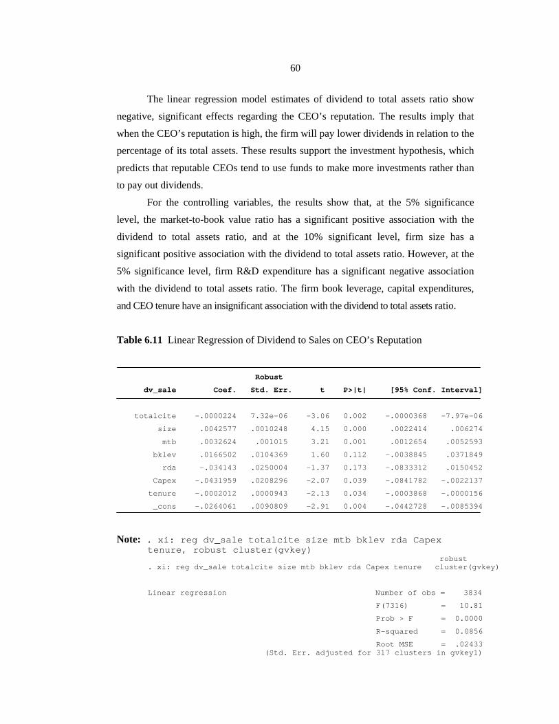
60
The linear regression model estimates of dividend to total assets ratio show
negative, significant effects regarding the CEO’s reputation. The results imply that
when the CEO’s reputation is high, the firm will pay lower dividends in relation to the
percentage of its total assets. These results support the investment hypothesis, which
predicts that reputable CEOs tend to use funds to make more investments rather than
to pay out dividends.
For the controlling variables, the results show that, at the 5% significance
level, the market-to-book value ratio has a significant positive association with the
dividend to total assets ratio, and at the 10% significant level, firm size has a
significant positive association with the dividend to total assets ratio. However, at the
5% significance level, firm R&D expenditure has a significant negative association
with the dividend to total assets ratio. The firm book leverage, capital expenditures,
and CEO tenure have an insignificant association with the dividend to total assets ratio.
Table 6.11 Linear Regression of Dividend to Sales on CEO’s Reputation
Robust
dv_sale Coef. Std. Err. t P>|t| [95% Conf. Interval]
totalcite -.0000224 7.32e-06 -3.06 0.002 -.0000368 -7.97e-06
size .0042577 .0010248 4.15 0.000 .0022414 .006274
mtb .0032624 .001015 3.21 0.001 .0012654 .0052593
bklev .0166502 .0104369 1.60 0.112 -.0038845 .0371849
rda -.034143 .0250004 -1.37 0.173 -.0833312 .0150452
Capex -.0431959 .0208296 -2.07 0.039 -.0841782 -.0022137
tenure -.0002012 .0000943 -2.13 0.034 -.0003868 -.0000156
_cons -.0264061 .0090809 -2.91 0.004 -.0442728 -.0085394
Note: . xi: reg dv_sale totalcite size mtb bklev rda Capex
tenure, robust cluster(gvkey)
. xi: reg dv_sale totalcite size mtb bklev rda Capex tenure robust cluster(gvkey)
Linear regression Number of obs = 3834
F(7316) = 10.81
Prob > F = 0.0000
R-squared = 0.0856
Root MSE = .02433 (Std. Err. adjusted for 317 clusters in gvkey1)
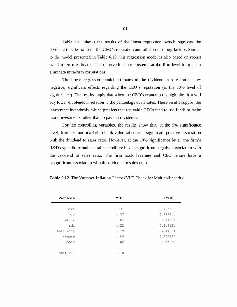
61
Table 6.11 shows the results of the linear regression, which regresses the
dividend to sales ratio on the CEO’s reputation and other controlling factors. Similar
to the model presented in Table 6.10, this regression model is also based on robust
standard error estimates. The observations are clustered at the firm level in order to
eliminate intra-firm correlations.
The linear regression model estimates of the dividend to sales ratio show
negative, significant effects regarding the CEO’s reputation (at the 10% level of
significance). The results imply that when the CEO’s reputation is high, the firm will
pay lower dividends in relation to the percentage of its sales. These results support the
investment hypothesis, which predicts that reputable CEOs tend to use funds to make
more investments rather than to pay out dividends.
For the controlling variables, the results show that, at the 5% significance
level, firm size and market-to-book value ratio has a significant positive association
with the dividend to sales ratio. However, at the 10% significance level, the firm’s
R&D expenditure and capital expenditure have a significant negative association with
the dividend to sales ratio. The firm book leverage and CEO tenure have a
insignificant association with the dividend to sales ratio.
Table 6.12 The Variance Inflation Factor (VIF) Check for Multicollinearity
Variable VIF 1/VIF
size 1.31 0.762521
mtb 1.27 0.788211
bklev 1.24 0.808637
rda 1.22 0.818131
totalcite 1.19 0.843664
tenure 1.03 0.967499
Capex 1.02 0.977032
Mean VIF 1.18
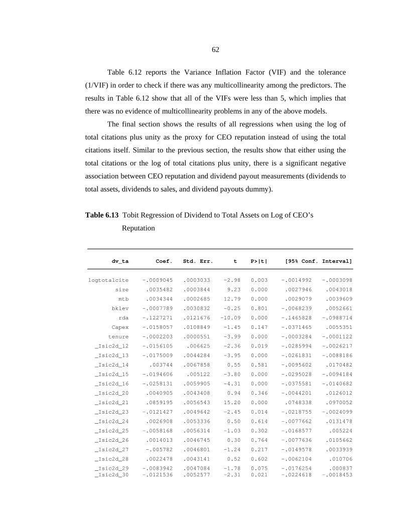
62
Table 6.12 reports the Variance Inflation Factor (VIF) and the tolerance
(1/VIF) in order to check if there was any multicollinearity among the predictors. The
results in Table 6.12 show that all of the VIFs were less than 5, which implies that
there was no evidence of multicollinearity problems in any of the above models.
The final section shows the results of all regressions when using the log of
total citations plus unity as the proxy for CEO reputation instead of using the total
citations itself. Similar to the previous section, the results show that either using the
total citations or the log of total citations plus unity, there is a significant negative
association between CEO reputation and dividend payout measurements (dividends to
total assets, dividends to sales, and dividend payouts dummy).
Table 6.13 Tobit Regression of Dividend to Total Assets on Log of CEO’s
Reputation
dv_ta Coef. Std. Err. t P>|t| [95% Conf. Interval]
logtotalcite -.0009045 .0003033 -2.98 0.003 -.0014992 -.0003098
size .0035482 .0003844 9.23 0.000 .0027946 .0043018
mtb .0034344 .0002685 12.79 0.000 .0029079 .0039609
bklev -.0007789 .0030832 -0.25 0.801 -.0068239 .0052661
rda -.1227271 .0121676 -10.09 0.000 -.1465828 -.0988714
Capex -.0158057 .0108849 -1.45 0.147 -.0371465 .0055351
tenure -.0002203 .0000551 -3.99 0.000 -.0003284 -.0001122
_Isic2d_12 -.0156105 .006625 -2.36 0.019 -.0285994 -.0026217
_Isic2d_13 -.0175009 .0044284 -3.95 0.000 -.0261831 -.0088186
_Isic2d_14 .003744 .0067858 0.55 0.581 -.0095602 .0170482
_Isic2d_15 -.0194606 .005122 -3.80 0.000 -.0295028 -.0094184
_Isic2d_16 -.0258131 .0059905 -4.31 0.000 -.0375581 -.0140682
_Isic2d_20 .0040905 .0043408 0.94 0.346 -.0044201 .0126012
_Isic2d_21 .0859195 .0056543 15.20 0.000 .0748338 .0970052
_Isic2d_23 -.0121427 .0049642 -2.45 0.014 -.0218755 -.0024099
_Isic2d_24 .0026908 .0053336 0.50 0.614 -.0077662 .0131478
_Isic2d_25 -.0058168 .0056314 -1.03 0.302 -.0168577 .005224
_Isic2d_26 .0014013 .0046745 0.30 0.764 -.0077636 .0105662
_Isic2d_27 -.005782 .0046801 -1.24 0.217 -.0149578 .0033939
_Isic2d_28 .0022478 .0043141 0.52 0.602 -.0062104 .010706
_Isic2d_29 -.0083942 .0047084 -1.78 0.075 -.0176254 .000837 _Isic2d_30 -.0121536 .0052577 -2.31 0.021 -.0224618 -.0018453
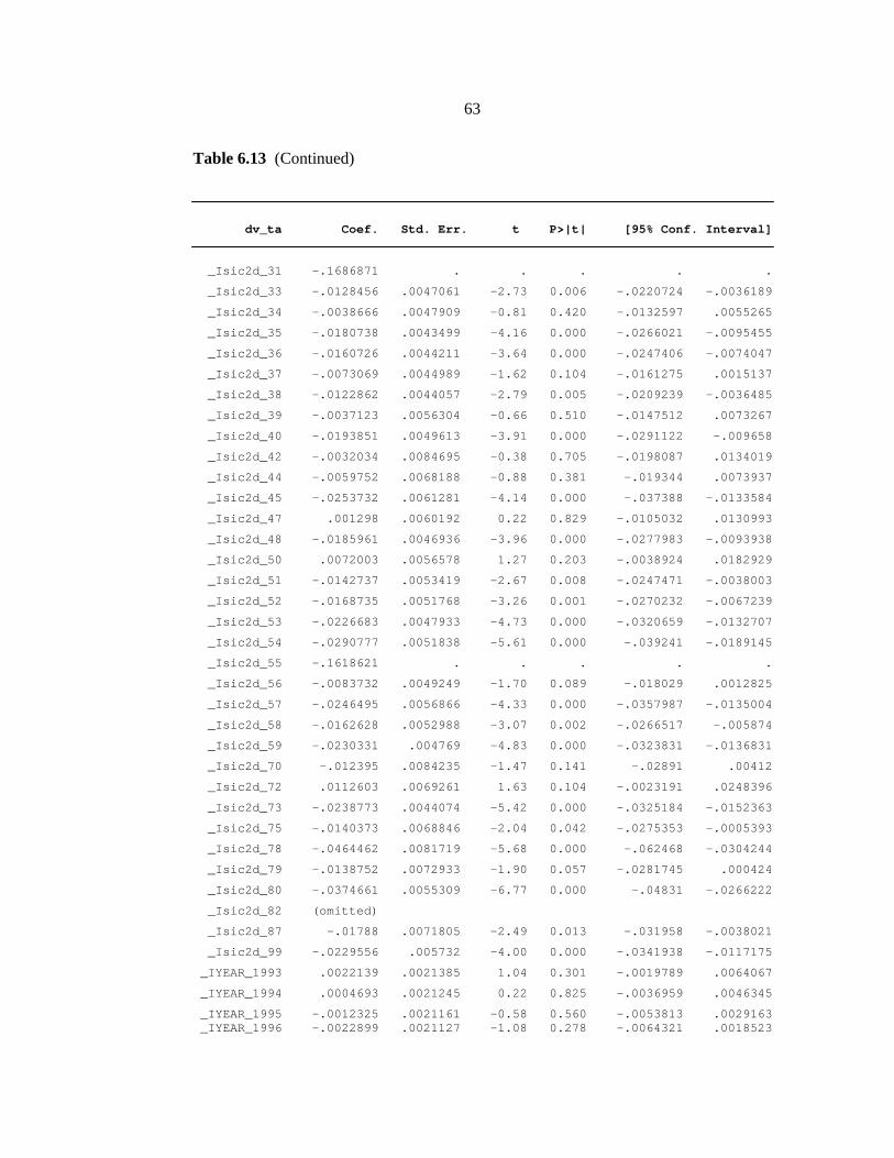
63
Table 6.13 (Continued)
dv_ta Coef. Std. Err. t P>|t| [95% Conf. Interval]
_Isic2d_31 -.1686871 . . . . .
_Isic2d_33 -.0128456 .0047061 -2.73 0.006 -.0220724 -.0036189
_Isic2d_34 -.0038666 .0047909 -0.81 0.420 -.0132597 .0055265
_Isic2d_35 -.0180738 .0043499 -4.16 0.000 -.0266021 -.0095455
_Isic2d_36 -.0160726 .0044211 -3.64 0.000 -.0247406 -.0074047
_Isic2d_37 -.0073069 .0044989 -1.62 0.104 -.0161275 .0015137
_Isic2d_38 -.0122862 .0044057 -2.79 0.005 -.0209239 -.0036485
_Isic2d_39 -.0037123 .0056304 -0.66 0.510 -.0147512 .0073267
_Isic2d_40 -.0193851 .0049613 -3.91 0.000 -.0291122 -.009658
_Isic2d_42 -.0032034 .0084695 -0.38 0.705 -.0198087 .0134019
_Isic2d_44 -.0059752 .0068188 -0.88 0.381 -.019344 .0073937
_Isic2d_45 -.0253732 .0061281 -4.14 0.000 -.037388 -.0133584
_Isic2d_47 .001298 .0060192 0.22 0.829 -.0105032 .0130993
_Isic2d_48 -.0185961 .0046936 -3.96 0.000 -.0277983 -.0093938
_Isic2d_50 .0072003 .0056578 1.27 0.203 -.0038924 .0182929
_Isic2d_51 -.0142737 .0053419 -2.67 0.008 -.0247471 -.0038003
_Isic2d_52 -.0168735 .0051768 -3.26 0.001 -.0270232 -.0067239
_Isic2d_53 -.0226683 .0047933 -4.73 0.000 -.0320659 -.0132707
_Isic2d_54 -.0290777 .0051838 -5.61 0.000 -.039241 -.0189145
_Isic2d_55 -.1618621 . . . . .
_Isic2d_56 -.0083732 .0049249 -1.70 0.089 -.018029 .0012825
_Isic2d_57 -.0246495 .0056866 -4.33 0.000 -.0357987 -.0135004
_Isic2d_58 -.0162628 .0052988 -3.07 0.002 -.0266517 -.005874
_Isic2d_59 -.0230331 .004769 -4.83 0.000 -.0323831 -.0136831
_Isic2d_70 -.012395 .0084235 -1.47 0.141 -.02891 .00412
_Isic2d_72 .0112603 .0069261 1.63 0.104 -.0023191 .0248396
_Isic2d_73 -.0238773 .0044074 -5.42 0.000 -.0325184 -.0152363
_Isic2d_75 -.0140373 .0068846 -2.04 0.042 -.0275353 -.0005393
_Isic2d_78 -.0464462 .0081719 -5.68 0.000 -.062468 -.0304244
_Isic2d_79 -.0138752 .0072933 -1.90 0.057 -.0281745 .000424
_Isic2d_80 -.0374661 .0055309 -6.77 0.000 -.04831 -.0266222
_Isic2d_82 (omitted)
_Isic2d_87 -.01788 .0071805 -2.49 0.013 -.031958 -.0038021
_Isic2d_99 -.0229556 .005732 -4.00 0.000 -.0341938 -.0117175
_IYEAR_1993 .0022139 .0021385 1.04 0.301 -.0019789 .0064067
_IYEAR_1994 .0004693 .0021245 0.22 0.825 -.0036959 .0046345
_IYEAR_1995 -.0012325 .0021161 -0.58 0.560 -.0053813 .0029163 _IYEAR_1996 -.0022899 .0021127 -1.08 0.278 -.0064321 .0018523
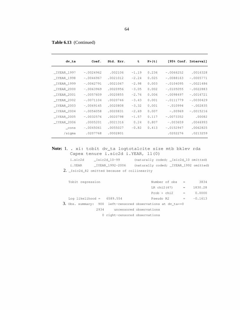
64
Table 6.13 (Continued)
dv_ta Coef. Std. Err. t P>|t| [95% Conf. Interval]
_IYEAR_1997 -.0024962 .002106 -1.19 0.236 -.0066252 .0016328
_IYEAR_1998 -.0046967 .0021012 -2.24 0.025 -.0088163 -.0005771
_IYEAR_1999 -.0062791 .0021067 -2.98 0.003 -.0104095 -.0021486
_IYEAR_2000 -.0063969 .0020956 -3.05 0.002 -.0105055 -.0022883
_IYEAR_2001 -.0057609 .0020855 -2.76 0.006 -.0098497 -.0016721
_IYEAR_2002 -.0071104 .0020746 -3.43 0.001 -.0111779 -.0030429
_IYEAR_2003 -.0069145 .0020808 -3.32 0.001 -.010994 -.002835
_IYEAR_2004 -.0056058 .0020831 -2.69 0.007 -.00969 -.0015216
_IYEAR_2005 -.0032576 .0020798 -1.57 0.117 -.0073352 .00082
_IYEAR_2006 .0005201 .0021316 0.24 0.807 -.003659 .0046993
_cons -.0045061 .0055027 -0.82 0.413 -.0152947 .0062825
/sigma .0207768 .0002801 .0202276 .0213259
Note: 1. . xi: tobit dv_ta logtotalcite size mtb bklev rda
Capex tenure i.sic2d i.YEAR, ll(0) i.sic2d _Isic2d_10-99 (naturally coded; _Isic2d_10 omitted)
i.YEAR _IYEAR_1992-2006 (naturally coded; _IYEAR_1992 omitted)
2. _Isic2d_82 omitted because of collinearity
Tobit regression Number of obs = 3834
LR chi2(67) = 1830.28
Prob > chi2 = 0.0000
Log likelihood = 6589.554 Pseudo R2 = -0.1613
3. Obs. summary: 900 left-censored observations at dv_ta<=0 2934 uncensored observations
0 right-censored observations
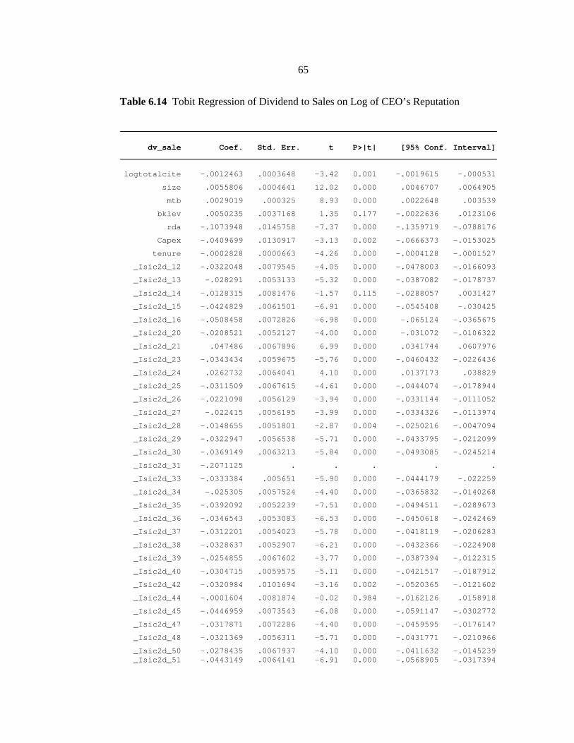
65
Table 6.14 Tobit Regression of Dividend to Sales on Log of CEO’s Reputation
dv_sale Coef. Std. Err. t P>|t| [95% Conf. Interval]
logtotalcite -.0012463 .0003648 -3.42 0.001 -.0019615 -.000531
size .0055806 .0004641 12.02 0.000 .0046707 .0064905
mtb .0029019 .000325 8.93 0.000 .0022648 .003539
bklev .0050235 .0037168 1.35 0.177 -.0022636 .0123106
rda -.1073948 .0145758 -7.37 0.000 -.1359719 -.0788176
Capex -.0409699 .0130917 -3.13 0.002 -.0666373 -.0153025
tenure -.0002828 .0000663 -4.26 0.000 -.0004128 -.0001527
_Isic2d_12 -.0322048 .0079545 -4.05 0.000 -.0478003 -.0166093
_Isic2d_13 -.028291 .0053133 -5.32 0.000 -.0387082 -.0178737
_Isic2d_14 -.0128315 .0081476 -1.57 0.115 -.0288057 .0031427
_Isic2d_15 -.0424829 .0061501 -6.91 0.000 -.0545408 -.030425
_Isic2d_16 -.0508458 .0072826 -6.98 0.000 -.065124 -.0365675
_Isic2d_20 -.0208521 .0052127 -4.00 0.000 -.031072 -.0106322
_Isic2d_21 .047486 .0067896 6.99 0.000 .0341744 .0607976
_Isic2d_23 -.0343434 .0059675 -5.76 0.000 -.0460432 -.0226436
_Isic2d_24 .0262732 .0064041 4.10 0.000 .0137173 .038829
_Isic2d_25 -.0311509 .0067615 -4.61 0.000 -.0444074 -.0178944
_Isic2d_26 -.0221098 .0056129 -3.94 0.000 -.0331144 -.0111052
_Isic2d_27 -.022415 .0056195 -3.99 0.000 -.0334326 -.0113974
_Isic2d_28 -.0148655 .0051801 -2.87 0.004 -.0250216 -.0047094
_Isic2d_29 -.0322947 .0056538 -5.71 0.000 -.0433795 -.0212099
_Isic2d_30 -.0369149 .0063213 -5.84 0.000 -.0493085 -.0245214
_Isic2d_31 -.2071125 . . . . .
_Isic2d_33 -.0333384 .005651 -5.90 0.000 -.0444179 -.022259
_Isic2d_34 -.025305 .0057524 -4.40 0.000 -.0365832 -.0140268
_Isic2d_35 -.0392092 .0052239 -7.51 0.000 -.0494511 -.0289673
_Isic2d_36 -.0346543 .0053083 -6.53 0.000 -.0450618 -.0242469
_Isic2d_37 -.0312201 .0054023 -5.78 0.000 -.0418119 -.0206283
_Isic2d_38 -.0328637 .0052907 -6.21 0.000 -.0432366 -.0224908
_Isic2d_39 -.0254855 .0067602 -3.77 0.000 -.0387394 -.0122315
_Isic2d_40 -.0304715 .0059575 -5.11 0.000 -.0421517 -.0187912
_Isic2d_42 -.0320984 .0101694 -3.16 0.002 -.0520365 -.0121602
_Isic2d_44 -.0001604 .0081874 -0.02 0.984 -.0162126 .0158918
_Isic2d_45 -.0446959 .0073543 -6.08 0.000 -.0591147 -.0302772
_Isic2d_47 -.0317871 .0072286 -4.40 0.000 -.0459595 -.0176147
_Isic2d_48 -.0321369 .0056311 -5.71 0.000 -.0431771 -.0210966
_Isic2d_50 -.0278435 .0067937 -4.10 0.000 -.0411632 -.0145239 _Isic2d_51 -.0443149 .0064141 -6.91 0.000 -.0568905 -.0317394
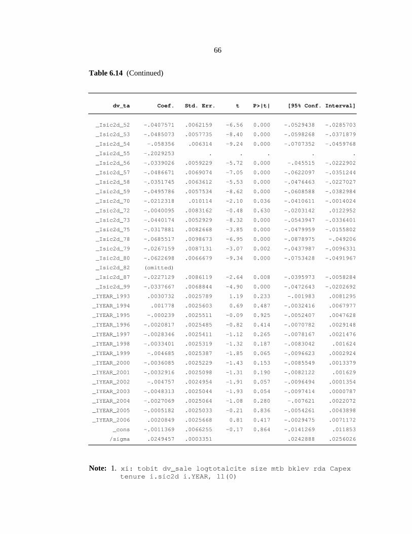
66
Table 6.14 (Continued)
dv_ta Coef. Std. Err. t P>|t| [95% Conf. Interval]
_Isic2d_52 -.0407571 .0062159 -6.56 0.000 -.0529438 -.0285703
_Isic2d_53 -.0485073 .0057735 -8.40 0.000 -.0598268 -.0371879
_Isic2d_54 -.058356 .006314 -9.24 0.000 -.0707352 -.0459768
_Isic2d_55 -.2029253 . . . . .
_Isic2d_56 -.0339026 .0059229 -5.72 0.000 -.045515 -.0222902
_Isic2d_57 -.0486671 .0069074 -7.05 0.000 -.0622097 -.0351244
_Isic2d_58 -.0351745 .0063612 -5.53 0.000 -.0476463 -.0227027
_Isic2d_59 -.0495786 .0057534 -8.62 0.000 -.0608588 -.0382984
_Isic2d_70 -.0212318 .010114 -2.10 0.036 -.0410611 -.0014024
_Isic2d_72 -.0040095 .0083162 -0.48 0.630 -.0203142 .0122952
_Isic2d_73 -.0440174 .0052929 -8.32 0.000 -.0543947 -.0336401
_Isic2d_75 -.0317881 .0082668 -3.85 0.000 -.0479959 -.0155802
_Isic2d_78 -.0685517 .0098673 -6.95 0.000 -.0878975 -.049206
_Isic2d_79 -.0267159 .0087131 -3.07 0.002 -.0437987 -.0096331
_Isic2d_80 -.0622698 .0066679 -9.34 0.000 -.0753428 -.0491967
_Isic2d_82 (omitted)
_Isic2d_87 -.0227129 .0086119 -2.64 0.008 -.0395973 -.0058284
_Isic2d_99 -.0337667 .0068844 -4.90 0.000 -.0472643 -.0202692
_IYEAR_1993 .0030732 .0025789 1.19 0.233 -.001983 .0081295
_IYEAR_1994 .001778 .0025603 0.69 0.487 -.0032416 .0067977
_IYEAR_1995 -.000239 .0025511 -0.09 0.925 -.0052407 .0047628
_IYEAR_1996 -.0020817 .0025485 -0.82 0.414 -.0070782 .0029148
_IYEAR_1997 -.0028346 .0025411 -1.12 0.265 -.0078167 .0021476
_IYEAR_1998 -.0033401 .0025319 -1.32 0.187 -.0083042 .001624
_IYEAR_1999 -.004685 .0025387 -1.85 0.065 -.0096623 .0002924
_IYEAR_2000 -.0036085 .0025229 -1.43 0.153 -.0085549 .0013379
_IYEAR_2001 -.0032916 .0025098 -1.31 0.190 -.0082122 .001629
_IYEAR_2002 -.004757 .0024954 -1.91 0.057 -.0096494 .0001354
_IYEAR_2003 -.0048313 .0025044 -1.93 0.054 -.0097414 .0000787
_IYEAR_2004 -.0027069 .0025064 -1.08 0.280 -.007621 .0022072
_IYEAR_2005 -.0005182 .0025033 -0.21 0.836 -.0054261 .0043898
_IYEAR_2006 .0020849 .0025668 0.81 0.417 -.0029475 .0071172
_cons -.0011369 .0066255 -0.17 0.864 -.0141269 .011853
/sigma .0249457 .0003351 .0242888 .0256026
Note: 1. xi: tobit dv_sale logtotalcite size mtb bklev rda Capex
tenure i.sic2d i.YEAR, ll(0)
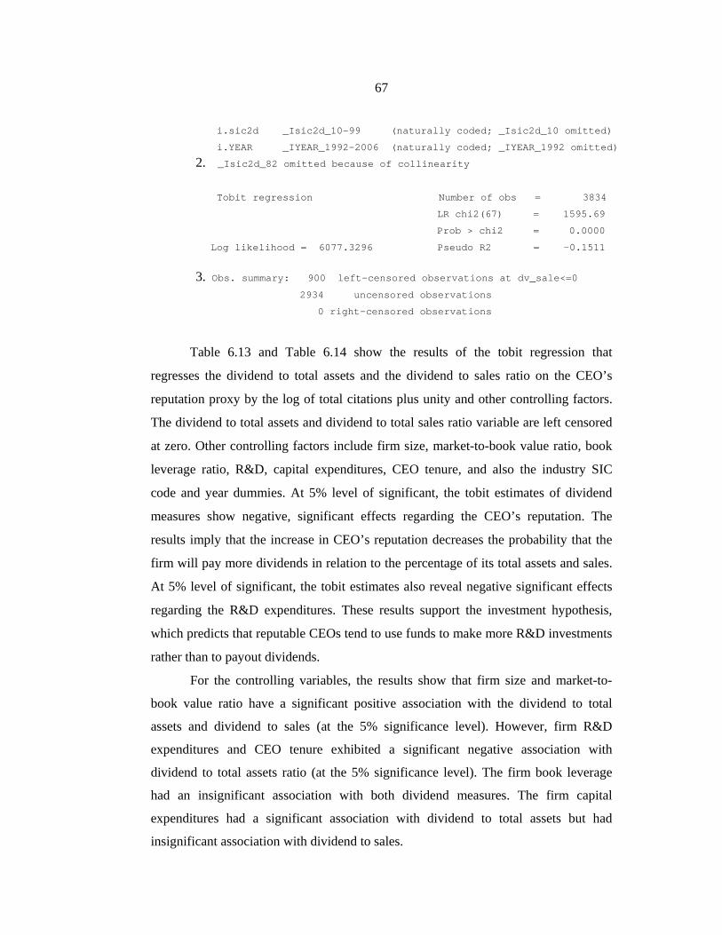
67
i.sic2d _Isic2d_10-99 (naturally coded; _Isic2d_10 omitted)
i.YEAR _IYEAR_1992-2006 (naturally coded; _IYEAR_1992 omitted)
2. _Isic2d_82 omitted because of collinearity
Tobit regression Number of obs = 3834
LR chi2(67) = 1595.69
Prob > chi2 = 0.0000
Log likelihood = 6077.3296 Pseudo R2 = -0.1511
3. Obs. summary: 900 left-censored observations at dv_sale<=0
2934 uncensored observations
0 right-censored observations
Table 6.13 and Table 6.14 show the results of the tobit regression that
regresses the dividend to total assets and the dividend to sales ratio on the CEO’s
reputation proxy by the log of total citations plus unity and other controlling factors.
The dividend to total assets and dividend to total sales ratio variable are left censored
at zero. Other controlling factors include firm size, market-to-book value ratio, book
leverage ratio, R&D, capital expenditures, CEO tenure, and also the industry SIC
code and year dummies. At 5% level of significant, the tobit estimates of dividend
measures show negative, significant effects regarding the CEO’s reputation. The
results imply that the increase in CEO’s reputation decreases the probability that the
firm will pay more dividends in relation to the percentage of its total assets and sales.
At 5% level of significant, the tobit estimates also reveal negative significant effects
regarding the R&D expenditures. These results support the investment hypothesis,
which predicts that reputable CEOs tend to use funds to make more R&D investments
rather than to payout dividends.
For the controlling variables, the results show that firm size and market-to-
book value ratio have a significant positive association with the dividend to total
assets and dividend to sales (at the 5% significance level). However, firm R&D
expenditures and CEO tenure exhibited a significant negative association with
dividend to total assets ratio (at the 5% significance level). The firm book leverage
had an insignificant association with both dividend measures. The firm capital
expenditures had a significant association with dividend to total assets but had
insignificant association with dividend to sales.
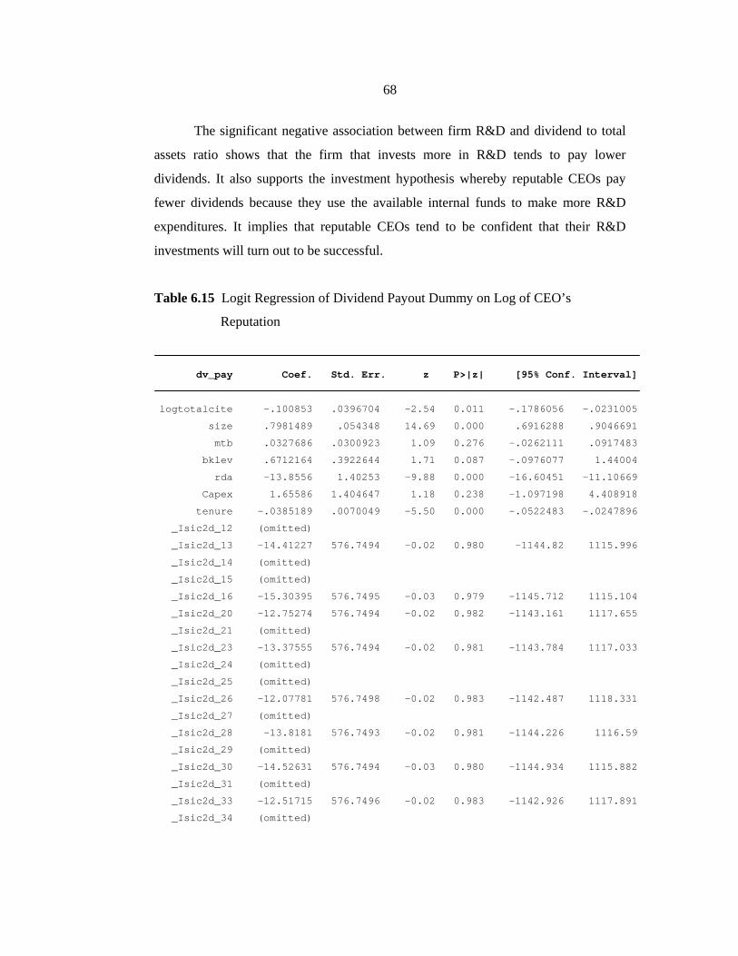
68
The significant negative association between firm R&D and dividend to total
assets ratio shows that the firm that invests more in R&D tends to pay lower
dividends. It also supports the investment hypothesis whereby reputable CEOs pay
fewer dividends because they use the available internal funds to make more R&D
expenditures. It implies that reputable CEOs tend to be confident that their R&D
investments will turn out to be successful.
Table 6.15 Logit Regression of Dividend Payout Dummy on Log of CEO’s
Reputation
dv_pay Coef. Std. Err. z P>|z| [95% Conf. Interval]
logtotalcite -.100853 .0396704 -2.54 0.011 -.1786056 -.0231005
size .7981489 .054348 14.69 0.000 .6916288 .9046691
mtb .0327686 .0300923 1.09 0.276 -.0262111 .0917483
bklev .6712164 .3922644 1.71 0.087 -.0976077 1.44004
rda -13.8556 1.40253 -9.88 0.000 -16.60451 -11.10669
Capex 1.65586 1.404647 1.18 0.238 -1.097198 4.408918
tenure -.0385189 .0070049 -5.50 0.000 -.0522483 -.0247896
_Isic2d_12 (omitted)
_Isic2d_13 -14.41227 576.7494 -0.02 0.980 -1144.82 1115.996
_Isic2d_14 (omitted)
_Isic2d_15 (omitted)
_Isic2d_16 -15.30395 576.7495 -0.03 0.979 -1145.712 1115.104
_Isic2d_20 -12.75274 576.7494 -0.02 0.982 -1143.161 1117.655
_Isic2d_21 (omitted)
_Isic2d_23 -13.37555 576.7494 -0.02 0.981 -1143.784 1117.033
_Isic2d_24 (omitted)
_Isic2d_25 (omitted)
_Isic2d_26 -12.07781 576.7498 -0.02 0.983 -1142.487 1118.331
_Isic2d_27 (omitted)
_Isic2d_28 -13.8181 576.7493 -0.02 0.981 -1144.226 1116.59
_Isic2d_29 (omitted)
_Isic2d_30 -14.52631 576.7494 -0.03 0.980 -1144.934 1115.882
_Isic2d_31 (omitted)
_Isic2d_33 -12.51715 576.7496 -0.02 0.983 -1142.926 1117.891
_Isic2d_34 (omitted)
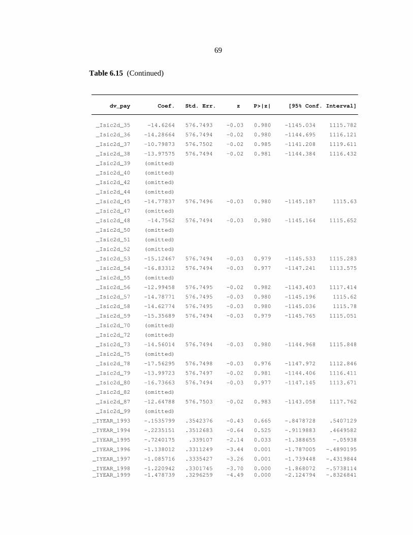
69
Table 6.15 (Continued)
dv_pay Coef. Std. Err. z P>|z| [95% Conf. Interval]
_Isic2d_35 -14.6264 576.7493 -0.03 0.980 -1145.034 1115.782
_Isic2d_36 -14.28664 576.7494 -0.02 0.980 -1144.695 1116.121
_Isic2d_37 -10.79873 576.7502 -0.02 0.985 -1141.208 1119.611
_Isic2d_38 -13.97575 576.7494 -0.02 0.981 -1144.384 1116.432
_Isic2d_39 (omitted)
_Isic2d_40 (omitted)
_Isic2d_42 (omitted)
_Isic2d_44 (omitted)
_Isic2d_45 -14.77837 576.7496 -0.03 0.980 -1145.187 1115.63
_Isic2d_47 (omitted)
_Isic2d_48 -14.7562 576.7494 -0.03 0.980 -1145.164 1115.652
_Isic2d_50 (omitted)
_Isic2d_51 (omitted)
_Isic2d_52 (omitted)
_Isic2d_53 -15.12467 576.7494 -0.03 0.979 -1145.533 1115.283
_Isic2d_54 -16.83312 576.7494 -0.03 0.977 -1147.241 1113.575
_Isic2d_55 (omitted)
_Isic2d_56 -12.99458 576.7495 -0.02 0.982 -1143.403 1117.414
_Isic2d_57 -14.78771 576.7495 -0.03 0.980 -1145.196 1115.62
_Isic2d_58 -14.62774 576.7495 -0.03 0.980 -1145.036 1115.78
_Isic2d_59 -15.35689 576.7494 -0.03 0.979 -1145.765 1115.051
_Isic2d_70 (omitted)
_Isic2d_72 (omitted)
_Isic2d_73 -14.56014 576.7494 -0.03 0.980 -1144.968 1115.848
_Isic2d_75 (omitted)
_Isic2d_78 -17.56295 576.7498 -0.03 0.976 -1147.972 1112.846
_Isic2d_79 -13.99723 576.7497 -0.02 0.981 -1144.406 1116.411
_Isic2d_80 -16.73663 576.7494 -0.03 0.977 -1147.145 1113.671
_Isic2d_82 (omitted)
_Isic2d_87 -12.64788 576.7503 -0.02 0.983 -1143.058 1117.762
_Isic2d_99 (omitted)
_IYEAR_1993 -.1535799 .3542376 -0.43 0.665 -.8478728 .5407129
_IYEAR_1994 -.2235151 .3512683 -0.64 0.525 -.9119883 .4649582
_IYEAR_1995 -.7240175 .339107 -2.14 0.033 -1.388655 -.05938
_IYEAR_1996 -1.138012 .3311249 -3.44 0.001 -1.787005 -.4890195
_IYEAR_1997 -1.085716 .3335427 -3.26 0.001 -1.739448 -.4319844
_IYEAR_1998 -1.220942 .3301745 -3.70 0.000 -1.868072 -.5738114 _IYEAR_1999 -1.478739 .3296259 -4.49 0.000 -2.124794 -.8326841
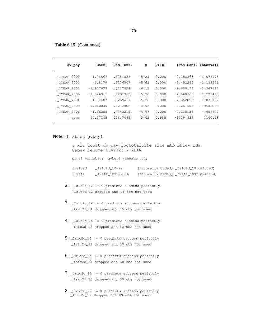
70
Table 6.15 (Continued)
dv_pay Coef. Std. Err. z P>|z| [95% Conf. Interval]
_IYEAR_2000 -1.71567 .3251057 -5.28 0.000 -2.352866 -1.078475
_IYEAR_2001 -1.8179 .3236507 -5.62 0.000 -2.452244 -1.183556
_IYEAR_2002 -1.977673 .3217028 -6.15 0.000 -2.608199 -1.347147
_IYEAR_2003 -1.926911 .3231965 -5.96 0.000 -2.560365 -1.293458
_IYEAR_2004 -1.71402 .3259411 -5.26 0.000 -2.352853 -1.075187
_IYEAR_2005 -1.610045 .3272806 -4.92 0.000 -2.251503 -.9685868
_IYEAR_2006 -1.56288 .3343215 -4.67 0.000 -2.218138 -.907622
_cons 10.57185 576.7495 0.02 0.985 -1119.836 1140.98
Note: 1. xtset gvkey1
. xi: logit dv_pay logtotalcite size mtb bklev rda Capex tenure i.sic2d i.YEAR
panel variable: gvkey1 (unbalanced)
i.sic2d _Isic2d_10-99 (naturally coded; _Isic2d_10 omitted)
i.YEAR _IYEAR_1992-2006 (naturally coded; _IYEAR_1992 omitted)
2. _Isic2d_12 != 0 predicts success perfectly
_Isic2d_12 dropped and 16 obs not used
3. _Isic2d_14 != 0 predicts success perfectly
_Isic2d_14 dropped and 15 obs not used
4. _Isic2d_15 != 0 predicts success perfectly
_Isic2d_15 dropped and 50 obs not used
5. _Isic2d_21 != 0 predicts success perfectly _Isic2d_21 dropped and 30 obs not used
6. _Isic2d_24 != 0 predicts success perfectly _Isic2d_24 dropped and 38 obs not used
7. _Isic2d_25 != 0 predicts success perfectly _Isic2d_25 dropped and 30 obs not used
8. _Isic2d_27 != 0 predicts success perfectly _Isic2d_27 dropped and 89 obs not used
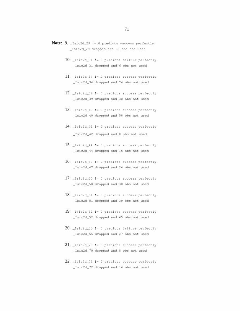
71
Note: 9. _Isic2d_29 != 0 predicts success perfectly _Isic2d_29 dropped and 88 obs not used
10. _Isic2d_31 != 0 predicts failure perfectly _Isic2d_31 dropped and 6 obs not used
11. _Isic2d_34 != 0 predicts success perfectly _Isic2d_34 dropped and 74 obs not used
12. _Isic2d_39 != 0 predicts success perfectly _Isic2d_39 dropped and 30 obs not used
13. _Isic2d_40 != 0 predicts success perfectly _Isic2d_40 dropped and 58 obs not used
14. _Isic2d_42 != 0 predicts success perfectly _Isic2d_42 dropped and 8 obs not used
15. _Isic2d_44 != 0 predicts success perfectly _Isic2d_44 dropped and 15 obs not used
16. _Isic2d_47 != 0 predicts success perfectly _Isic2d_47 dropped and 24 obs not used
17. _Isic2d_50 != 0 predicts success perfectly _Isic2d_50 dropped and 30 obs not used
18. _Isic2d_51 != 0 predicts success perfectly _Isic2d_51 dropped and 39 obs not used
19. _Isic2d_52 != 0 predicts success perfectly _Isic2d_52 dropped and 45 obs not used
20. _Isic2d_55 != 0 predicts failure perfectly _Isic2d_55 dropped and 27 obs not used
21. _Isic2d_70 != 0 predicts success perfectly _Isic2d_70 dropped and 8 obs not used
22. _Isic2d_72 != 0 predicts success perfectly _Isic2d_72 dropped and 14 obs not used
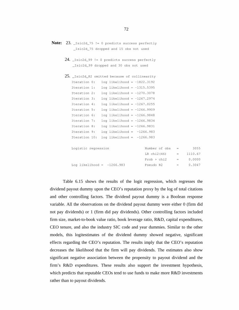
72
Note: 23. _Isic2d_75 != 0 predicts success perfectly _Isic2d_75 dropped and 15 obs not used
24. _Isic2d_99 != 0 predicts success perfectly _Isic2d_99 dropped and 30 obs not used
25. _Isic2d_82 omitted because of collinearity Iteration 0: log likelihood = -1822.3192
Iteration 1: log likelihood = -1315.5395
Iteration 2: log likelihood = -1270.3078
Iteration 3: log likelihood = -1267.2974
Iteration 4: log likelihood = -1267.0255
Iteration 5: log likelihood = -1266.9909
Iteration 6: log likelihood = -1266.9848
Iteration 7: log likelihood = -1266.9834
Iteration 8: log likelihood = -1266.9831
Iteration 9: log likelihood = -1266.983
Iteration 10: log likelihood = -1266.983
Logistic regression Number of obs = 3055
LR chi2(46) = 1110.67
Prob > chi2 = 0.0000
Log likelihood = -1266.983 Pseudo R2 = 0.3047
Table 6.15 shows the results of the logit regression, which regresses the
dividend payout dummy upon the CEO’s reputation proxy by the log of total citations
and other controlling factors. The dividend payout dummy is a Boolean response
variable. All the observations on the dividend payout dummy were either 0 (firm did
not pay dividends) or 1 (firm did pay dividends). Other controlling factors included
firm size, market-to-book value ratio, book leverage ratio, R&D, capital expenditures,
CEO tenure, and also the industry SIC code and year dummies. Similar to the other
models, this logitestimates of the dividend dummy showed negative, significant
effects regarding the CEO’s reputation. The results imply that the CEO’s reputation
decreases the likelihood that the firm will pay dividends. The estimates also show
significant negative association between the propensity to payout dividend and the
firm’s R&D expenditures. These results also support the investment hypothesis,
which predicts that reputable CEOs tend to use funds to make more R&D investments
rather than to payout dividends.
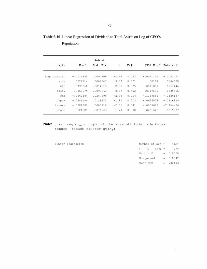
73
Table 6.16 Linear Regression of Dividend to Total Assets on Log of CEO’s
Reputation
Robust
dv_ta Coef. Std. Err. t P>|t| [95% Conf. Interval]
logtotalcite -.0011354 .0004969 -2.28 0.023 -.0021131 -.0001577
size .0028114 .0008343 3.37 0.001 .00117 .0044528
mtb .0039668 .0014118 2.81 0.005 .0011891 .0067446
bklev .0060979 .0090763 0.67 0.502 -.0117597 .0239555
rda -.0662884 .0267699 -2.48 0.014 -.1189581 -.0136187
Capex -.0381494 .0129375 -2.95 0.003 -.0636038 -.0126949
tenure -.0001881 .0000918 -2.05 0.041 -.0003688 -7.45e-06
_cons -.0121281 .0071343 -1.70 0.090 -.0261648 .0019087
Note: . xi: reg dv_ta logtotalcite size mtb bklev rda Capex tenure, robust cluster(gvkey)
Linear regression Number of obs = 3834
F( 7, 316) = 7.74
Prob > F = 0.0000
R-squared = 0.0942
Root MSE = .02103
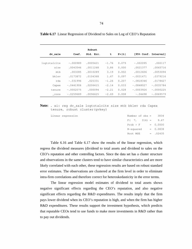
74
Table 6.17 Linear Regression of Dividend to Sales on Log of CEO’s Reputation
Robust
dv_sale Coef. Std. Err. t P>|t| [95% Conf. Interval]
logtotalcite -.000989 .0005621 -1.76 0.079 -.002095 .000117
size .0043546 .0011268 3.86 0.000 .0021377 .0065716
mtb .003285 .0010289 3.19 0.002 .0012606 .0053094
bklev .0173872 .0104368 1.67 0.097 -.0031471 .0379216
rda -.031996 .025331 -1.26 0.207 -.0818346 .0178427
Capex -.0441906 .0206415 -2.14 0.033 -.0848027 -.0035784
tenure -.0002075 .000094 -2.21 0.028 -.0003926 -.0000225
_cons -.0259689 .0096625 -2.69 0.008 -.04498 -.0069579
Note: . xi: reg dv_sale logtotalcite size mtb bklev rda Capex tenure, robust cluster(gvkey) Linear regression Number of obs = 3834
F( 7, 316) = 9.67
Prob > F = 0.0000
R-squared = 0.0838
Root MSE = .02435
Table 6.16 and Table 6.17 show the results of the linear regression, which
regress the dividend measures (dividend to total assets and dividend to sales on the
CEO’s reputation and other controlling factors. Since the data set has a cluster structure
and observations in the same clusters tend to have similar characteristics and are more
likely correlated with each other, these regression results are based on robust standard
error estimates. The observations are clustered at the firm level in order to eliminate
intra-firm correlations and therefore correct for heteroskedasticity in the error terms.
The linear regression model estimates of dividend to total assets shows
negative significant effects regarding the CEO’s reputation, and also negative
significant effects regarding the R&D expenditures. The results imply that the firm
pays lower dividend when its CEO’s reputation is high, and when the firm has higher
R&D expenditures. These results support the investment hypothesis, which predicts
that reputable CEOs tend to use funds to make more investments in R&D rather than
to pay out dividends.
CHAPTER 7
CONCLUSION
This research explores the relationship between CEO reputation and firm
dividend payouts. The existing hypotheses suggest that firms that have CEO with
higher reputation may have more, or less, or no relevancy to dividend payout.
One argument states that reputable CEO may pay more dividends because they
are afraid to make risky investment that could ruin their reputation if the investment
turns to be a failure. However, the counter argument states that reputable CEO may
pay lower dividends because they are confident that their investments will be
successful and so they would like to make more investment.
Using press coverage (media counts) to proxy for CEO reputation, this study
conducts empirical tests and finds that firms with reputable CEOs tend to make more
investment in R&D and tend to pay lower dividends. The logistic regression shows
that firms with more reputable CEOs are less likely to payout dividends.
Although the press coverage may refer to CEO’s name in either positive or
negative way, Francis et al. (2008) ensure that the number of citations is not a
reflection of CEO infamy as opposed to reputation by conducting three validation
checks. First, when the articles are randomly selected, the tone is favorable toward the
CEO 95% of the time. Second, the number of press coverage is correlated with a
proxy for reputation used by Milbourn (2003) and Rajgopal et al. (2006) who used the
numbers of CEOs appointed from outside the firm as a proxy for reputation. Third,
the number of citations is highly correlated with explicit recognition of the CEO by
the “top CEO” lists compiled by various sources. The results of these validity checks
justify the use of press coverage or total citations as a measure of the CEO reputation.
According to these results, it is reasonable to use the press coverage as a proxy for
CEO reputation.
The results remain robust and significant at 5% level for both tobit regression
and logistic regression, and also after controlling for other firm’s policy variables,

76
CEO variables, and firm’s characteristic variables. Because the total citations are not
normally distributed and are relatively in large scale compared to the dividend
measurements, the last section reports the regression analysis using the log of total
citations plus unity instead of the total citations. In both cases, the regressions yield
the same results. Our results have important implications because they show that a
manager-specific characteristic has a significant influence on corporate dividend
payouts.
BIBLIOGRAPHY
Allen, Franklin and Michaely, Roni. 2002. Payout Policy. The Working Paper
Series is Made Possible by a Generous Grant from the Alfred P. Sloan
Foundation. Financial Institutions Center. Retrieved July 20, 2011 from
http://fic.wharton.upenn.edu/fic/papers/01/0121.pdf
Allen, Franklin; Bernardo, Antonio and Welch, Ivo. 2000. A Theory of Dividends Based
on Tax Clientele. The Journal of Finance. 55 (December): 2499-2536.
Ambarish, Ramasastry; Kose, John and Joseph, Williams. 1987. Efficient Signaling
with Dividends and Investments. The Journal of Finance. 42 (June): 321-
343.
Amihud, Yakov and Baruch Lev. 1981. Risk Reduction as a Managerial Motive for
Conglomerate Mergers. The Bell Journal of Economics. 12 (2): 605-617.
Baker, Malcolm and Jeffrey, Wurgler. 2004a. A Catering Theory of Dividends.
The Journal of Finance. 59 (June): 1125-1165.
Baker, Malcolm and Jeffrey, Wurgler. 2004b. Appearing and Disappearing
Dividends: The Link to Catering Incentives. Journal of Financial
Economics. 73 (August): 271-288.
Barclay, M.; Smith, C. and Watts, R. 1995. The Determinants of Corporate Leverage
and Dividend Policies. Journal of Applied Corporate Finance.
7 (Winter): 4-19.
Baum, Christopher F. 2006. An Introduction to Modern Econometrics Using
STATA. College Station, Tex.: Stata Press.
Bertrand, Marianne and Schoar, Antoinette. 2003. Managing with Style: The Effect
of Managers on Firm Policies. The Quarterly Journal of Economics.
118 (4): 1169-1208.
Bernheim, Douglas. 1991. Tax Policy and the Dividend Puzzle. Rand Journal of
Economics. 22 (Winter): 455-476.
Bhattacharya, Sudipto. 1979. Imperfect Information, Dividend Policy, and ‘The Bird
In The Hand’ Fallacy. Bell Journal of Economics. 10 (1): 259-270.
78
Brickley, James A.; Coles, Jeffrey L. and Linck, James S. 1999. What Happens to
CEOs After They Retire? New Evidence on Career Concerns, Horizon
Problems, and CEO Incentives. Journal of Financial Economics.
52 (June): 341-377.
Brooks, Chris. 2008. Introductory Econometrics for Finance. 2nd ed.
New York: Cambridge University Press.
Camerer, C. and Lovallo, D. 1999. Overconfidence and Excess Entry: An
Experimental Approach. American Economic Review. 89 (March): 306-
318.
Chatterjee, C. and. Hambrick, D. 2007. It’s all About Me: Narcissistic Chief Executive
Officers and Their Effects on Company Strategy and Performance. Administrative
Science Quarterly. 52 (September): 351-386.
Chevalier, Judith and Ellison, Glenn. 1999. Are Some Mutual Fund Managers Better
Than Others? Cross-Sectional Patterns in Behavior and Performance.
The Journal of Finance. 54 (June): 875-899.
Denis, David J. and Osobov, Igor V. 2005. Disappearing Dividends, Catering
Incentives and Agency Costs: International Evidence. Retrieved
August 13, 2011 from http://ssrn.com/abstract=778024 or
http://dx.doi.org/10.2139/ssrn.778024
DiMaggio, P. and Powell,W. 1983. The Iron Cage Revisited: Institutional
Isomorphism and Collective Rationality in Organizational Fields.
American Sociological Review. 48 (April): 147-160.
Easterbrook, Frank H. 1984. Two Agency-Cost Explanations of Dividends.
American Economic Review. 74 (September): 650-659.
Fama, E. and French, K. 2001. Disappearing Dividends: Changing Firm
Characteristics or Lower Propensity to Pay?. Journal of Financial
Economics. 60 (April): 3-43.
Feldstein, S. and Green, J. 1983. Why do Companies Pay Dividends?.
The American Economic Review. 73 (1): 17-30.
Ferris, S.; Jagannathan, M. and Pritchar, A. C. 2003. Too Busy to Mind the
Business?. Monitoring by Directors with Multiple Appointments.
The Journal of Finance. 58 (June): 1087-1112.
79
Ferris, S. P.; Narayanan Jayaraman, and Sanjiv Sabherwal. 2009. Catering Effects in
Corporate Dividend Policy: The International Evidence. Journal of
Banking and Finance. 33 (9): 1730-1738.
Francis, J.; Huang, Allen H.; Rajgopal, S. and Zang, Amy Y. 2008. CEO Reputation
and Earnings Quality. Contemporary Accounting Research.
25 (Spring): 109-147.
Gaines-Ross, L. 2003. CEO Capital: A Guide to Building CEO Reputation and
Company success. Hobokin, N.J.: Wiley & Sons.
Gao, L. and Sudarsanam, P. 2005. Executive Compensation, Hubris, Corporate
Governance: Impact on Managerial Risk Taking and Value Creation
in UK High-Tech and Low-Tech Acquisitions. Retrieved August
13,2011 from http://www.efmaefm.org/efmsympo2005/
accepted_papers/33-Sudi_Sudarsanam_compensation_paper.pdf
Gilson, S. C. 1989. Management Turnover and Financial Distress. Journal of
Financial Economics. 25 (December): 241-262.
Gilson, S. C. 1990. Bankruptcy, Boards, Banks, and Blockholders: Evidence on
Changes in Corporate Ownership and Control When Firms Default.
Journal of Financial Economics. 27 (October): 355-387.
Graham, John R. and Campbell R. Harvey. 2001. The Theory and Practice of
Corporate Finance: Evidence from the Field. Journal of Financial
Economics. 60 (May): 187-243.
Grossman, Sanford J. and Hart, Oliver D. 1980. Takeover Bids, the Free-Rider
Problem, and the Theory of the Corporation. Bell Journal of Economics.
11 (Spring): 42-64.
Grullon, Gustavo and Michaely, Roni. 2002. Dividends, Share Repurchases and the
Substitution Hypothesis. The Journal of Finance. 62, 4 (August): 1649-1684.
Gustavo Grullon, Roni Michaely, and Bhaskaran Swaminathan. 2002. Are Dividend
Changes a Sign of Firm Maturity?. The Journal of Business.
75 (3): 387-424.
Hannan, M. and Freeman, J. 1977. The Population Ecology of Organizations.
American Journal of Sociology. 82 (March): 929-964.

80
Harris, M. and Raviv, A. 1991. The Theory of Capital Structure. The Journal of
Finance. 46 (March): 297-355.
Hirshleifer, D. and Thakor, A. 1992. Managerial Conservatism, Project Choice and
Debt. The Review of Financial Studies. 5 (3): 437-470.
Hribar, P. and Yang, H. 2007. Does CEO Overconfidence Affect Management
Forecasting and Subsequent Earnings Management?. Working Paper.
Tippie College of Business, University of Iowa.
Hoberg, G. and Prabhala, N. 2005. Disappearing Dividends: The Importance of
Idiosyncratic Risk and the Irrelevance of Catering. Working Paper.
University of Maryland.
Holder, M.; Langrehr, F. and Hexter, L. 1998. Dividend Policy Determinants: An
Investigation of the Influence of Stakeholder Theory. Financial
Management. 27 (Autumn): 73-82.
Holmstrom, B. and Costa, J. R. 1986. Managerial Incentives and Capital Management. The
Quarterly Journal of Economics. 101 (November): 835-860.
Hu, A. and Kumar, P. 2004. Managerial Entrenchment and Payout Policy. Journal
of Financial and Quantitative Analysis. 39 (December): 759-790.
Jensen, Michael C. 1986. Agency Costs of Free Cash Flow, Corporate Finance, and
Takeovers. American Economic Review. 76 (2): 323-329.
Jensen, Michael C. and Meckling, William H. 1976. Theory of the Firm: Managerial
Behavior, Agency Costs and Ownership Structure. Journal of Financial
Economics. 3 (October): 305-360.
Jensen, Gerald R.; Donald P. Solberg and Thomas S. Zorn. 1992. Simultaneous
Determination of Insider Ownership, Debt, and Dividend Policies.
Journal of Financial and Quantitative Analysis. 27 (June): 247-263.
Jin, L. and Kothari, S. P. 2006. Effects of Personal Taxes on Managers' Decision to Sell
Unrestricted Equity. Working Paper. Harvard University and MIT.
John, Kose and Williams, Joseph. 1985. Dividends, Dilution, and Taxes: a Signaling
Equilibrium. Journal of Finance. 40 (September): 1053-1070.
Kahneman, D. and Lovallo, D. 1993. Timid Choices and Bold Forecasts: a Cognitive
Perspective on Risk Taking. Management Science. 39 (January): 17-31.
81
Kaplan, S. and Reihus, D. 1990. Outside Directorships and Corporate Performance.
Journal of Financial Economics. 27 (2): 389-410.
Kutner, Michael H.; Nachtsheim, Christopher J.; Neter, John and William, Li. 2005.
Applied Linear Statistical Models. 5th ed. Boston: McGraw-Hill Irwin.
Li, W. and Lie, E. 2006. Dividend Changes and Catering Incentives. Journal of
Financial Economics. 80 (May): 293-308.
Liu, Yixin, Zhang, Yilei and Pornsit Jiraporn. 2011. CEO Reputation and
Corporate Risk Taking. Working Paper. Pennsylvania State University.
Malmendier, U. and Tate, G. 2005a. CEO Overconfidence and Corporate
Investment. Journal of Finance. 60 (December): 2661-2700.
Malmendier, U. and Tate, G. 2005b. Who Makes Acquisitions?. CEO
Overconfidence and the Market's Reaction. Working Paper. Stanford
University and University of Pennsylvania.
March, J. and Shapira, Z. 1987. Managerial Perspectives on Risk and Risk Taking.
Management Science. 33 (November): 1404-1418.
Milbourn, T. 2003. CEO Reputation and Stock-Based Compensation. Journal of
Financial Economics. 68 (May): 233-263.
Miller, Merton and Modigliani, Franco. 1961. Dividend Policy, Growth and the
Valuation of Shares. Journal of Business. 34 (October): 411-433.
Miller, Merton and Rock, Kevin. 1985. Dividend Policy Under Asymmetric
Information. Journal of Finance. 40 (September): 1031-1051.
Myers, Stewart C. 1977. Determinants of Corporate Borrowing. Journal of
Financial Economics. 5 (Noverber): 147-175.
Nosic, A. and Weber, M. 2010. How Risky do I Invest: The Role of Risk Attitudes,
Risk Perceptions, and Overconfidence. Decision Analysis. 7 (September):
282-301.
Polk, C. and Sapienza, P. 2004. The Real Effects of Investor Sentiment. NBER
Working Paper 10563.
Rajgopal, Shivaram; Shevlin, Terry and Zamora, Valentina. 2006. CEO’s Outside
Employment Opportunities and Lack of Relative Performance Evaluation.
Journal of Finance. 61 (4): 1813-1844.
82
Redding, L. S. 1997. Firm Size and Dividend Payouts. Journal of Financial
Intermediation. 6 (July): 224-248.
Richardson, Scott A.; Tuna, A Irem and Wysocki, Peter D. 2003. Accounting for
Taste: Board Member Preferences and Corporate Policy. MIT
SloanWorking paper No. 4307-03.
Ross, S. 1977. The Determination of Financial Structure: The Incentive Signaling
Approach. Bell Journal of Economics. 8 (Spring): 23-40.
Rozeff, M. 1982. Growth, Beta, and Agency Costs as Determinants of Dividend
Payout ratios. Journal of Financial Research. 5 (3): 249-259.
Shane, S. and Stuart, T. 2002. Organizational Endowments and The Performance of
University Start-Ups. Management Science. 48 (January): 154-170.
Shefrin, M. and Statman, M. 1984. Explaining Investor Preference for Cash
Dividends. Journal of Financial Economics. 13 (June): 253-282.
Sitkin, S. and Pablo, A. 1992. Re-conceptualizing the Determinants of Risk
Behavior. Academy of Management Review. 17 (January): 9-38.
Tsuji, Chikashi. 2010. A Test of the Catering Theory of Dividends: The Case of the
Japanese Electric Appliances Industry. Journal of Management
Research. 2 (2): 2-16.
Twite, G. 2001. Capital Structure Choices and Taxes: Evidence from the Australian
Dividend Imputation Tax System. International Review of Finance.
2 (December): 217-234.
Whisenant, S.; Sankaraguruswamy, S. and Raghunandan, K. 2003. Evidence on the
Joint Determination of Audit and Non-Audit Fees. Journal of
Accounting Research. 41 (September): 721-744.
Williams, Joseph. 1988. Efficient Signaling with Dividends, Investment, and Stock
Repurchases. Journal of Finance. 43 (July): 737-747.

APPENDIX

84
THE STATA CODE
The STATA code
Table 5
oneway totalcite dv_pay, tabulate
table 6
ttest totalcite, by(dv_pay) unequal Welch
table 7
. xi: tobit dv_ta totalcite size mtb bklev rda Capex tenure i.sic2d i.YEAR, ll(0)
Table 8
. xi: tobit dv_sale totalcite size mtb bklev rda Capex tenure i.sic2d i.YEAR, ll(0)
Table 9
xtset gvkey1
. xi: logit dv_pay totalcite size mtb bklev rda Capex tenure i.sic2d i.YEAR
Table 10
mfx compute
Table 11
. xtlogit dv_pay totalcite size mtb bklev rda Capex tenure
Table 12
mfx compute
Table 13
. xtlogit dv_pay totalcite size mtb bklev rda Capex tenure, i(gvkey1) fe
mfx compute **cannot
Table 14
. xi: reg dv_ta totalcite size mtb bklev rda Capex tenure, robust cluster(gvkey)
Table 15
. xi: reg dv_sale totalcite size mtb bklev rda Capex tenure, robust cluster(gvkey)
Table 16
vif
Find the marginal effect at each quantile and median
85
xtset gvkey1 . xi: logit dv_pay totalcite size mtb bklev rda Capex tenure i.sic2d i.YEAR summarize totalcite, detail Replace the following “0” with the number of total citations at percentile 25, percentile 50, percentile 75, and maximum (quantile 1, 2, 3, and 4) mfx compute, at(totalcite = 0) mfx compute, at(totalcite = 0) mfx compute, at(totalcite = 0) mfx compute, at(totalcite = 0) Find the marginal effect at each quantile and median . xtlogit dv_pay totalcite size mtb bklev rda Capex tenure summarize totalcite, detail
Replace the following “0” with the number of total citations at percentile 25, percentile 50, percentile 75, and maximum (quantile 1, 2, 3, and 4)
mfx compute, at(totalcite = 0) mfx compute, at(totalcite = 0) mfx compute, at(totalcite = 0) mfx compute, at(totalcite = 0) For the logtotalcite
Table 17 . xi: tobit dv_ta logtotalcite size mtb bklev rda Capex tenure i.sic2d i.YEAR, ll(0) Table 18 . xi: tobit dv_sale logtotalcite size mtb bklev rda Capex tenure i.sic2d i.YEAR, ll(0) Table 19 xtset gvkey1 . xi: logit dv_pay logtotalcite size mtb bklev rda Capex tenure i.sic2d i.YEAR Table 20 . xi: reg dv_ta logtotalcite size mtb bklev rda Capex tenure, robust cluster(gvkey) Table 21 . xi: reg dv_sale logtotalcite size mtb bklev rda Capex tenure, robust cluster(gvkey)
BIOGRAPHY
NAME Danai Likitratcharoen
ACADEMIC BACKGROUND Bachelor Degree of Engineering, Major Civil
Engineer, Chiangmai University, Thailand
Master of Technology Management, University
of New South Wales, Australia
PRESENT POSITION AVP Market Risk Department, Krungthai Bank
EXPERIENCES Trader, Krungthai Bank
Market Risk Officer, Siam Commercial Bank