imperfect monitoring and impermanent reputations · imperfect monitoring and impermanent...
TRANSCRIPT

Imperfect Monitoring and
Impermanent Reputations∗
Martin W. CrippsOlin School of Business
Washington University in St. LouisSt. Louis, MO 63130-4899
George J. MailathDepartment of EconomicsUniversity of Pennsylvania
3718 Locust WalkPhiladelphia, PA [email protected]
Larry SamuelsonDepartment of EconomicsUniversity of Wisconsin1180 Observatory DriveMadison, WI [email protected]
July 30, 2002
Abstract
We study the long-run sustainability of reputations in games with im-perfect public monitoring. It is impossible to maintain a permanentreputation for playing a strategy that does not eventually play an equi-librium of the game without uncertainty about types. Thus, a playercannot indefinitely sustain a reputation for non-credible behavior inthe presence of imperfect monitoring.
Journal of Economic Literature Classification Numbers C70, C78.
Keywords: Reputation, Imperfect Monitoring, Repeated Game, Com-mitment.
∗We thank the audiences at many seminars for their helpful comments and the NationalScience Foundation (under grants SES-0095768 and SES-9911219) for financial support.
Contents
1 Introduction 1
2 Illustrative Example and Related Literature 4
3 The Model 73.1 The Complete-Information Game . . . . . . . . . . . . . . . . 73.2 Never an Equilibrium Strategy in the Long Run . . . . . . . . 93.3 The Incomplete-Information Game . . . . . . . . . . . . . . . 12
4 Impermanent Reputations 134.1 The “Easy” Case: Player 2’s Beliefs Known . . . . . . . . . . 144.2 The Harder Case: Player 2’s Beliefs Unknown . . . . . . . . . 164.3 Asymptotic Equilibrium Play . . . . . . . . . . . . . . . . . . 174.4 Impermanent Restrictions on Behavior . . . . . . . . . . . . . 20
5 Proofs of Theorems 1 and 2 215.1 Preliminary results . . . . . . . . . . . . . . . . . . . . . . . . 21
5.1.1 Player 2’s Posterior Beliefs . . . . . . . . . . . . . . . 215.1.2 Player 2’s Behavior . . . . . . . . . . . . . . . . . . . . 245.1.3 Beliefs about Player 2’s Beliefs . . . . . . . . . . . . . 24
5.2 Proof of Theorem 1 (the “Easy” Case) . . . . . . . . . . . . 265.3 Proof of Theorem 2 (the Harder Case) . . . . . . . . . . . . . 27
6 Imperfect Private Monitoring 35
7 Many Types 37
8 Two Long-Run Players 39
A Appendix 40A.1 Proof of Theorem 3 (Section 4.3) . . . . . . . . . . . . . . . . 40A.2 Proof of Theorem 4 (Section 4.4) . . . . . . . . . . . . . . . . 42A.3 Verification of (16) (Section 5.1.3) . . . . . . . . . . . . . . . 44
1 Introduction
The adverse selection approach to reputations is central to the study of long-run relationships. In the complete-information finitely-repeated prisoners’dilemma or chain store game, for example, the intuitively obvious outcomeis inconsistent with equilibrium. However, if some player’s characteristicsare not common knowledge, that player may acquire a reputation for co-operating or playing “tough,” rendering the intuitive outcome consistentwith equilibrium (Kreps, Milgrom, Roberts, and Wilson (1982), Kreps andWilson (1982), and Milgrom and Roberts (1982)). In other situations, rep-utation effects impose intuitive limits on the set of equilibria by imposing“high” lower bounds on equilibrium payoffs (Fudenberg and Levine (1989,1992)).
We explore the long-run possibilities for reputation effects in imperfectmonitoring games with a long-lived player facing a sequence of short-livedplayers. The “short-run” reputation effects in these games are relativelyclear-cut. In the absence of incomplete information about the long-livedplayer, there are many equilibria and the long-lived player’s equilibriumpayoff is bounded below that player’s Stackelbeg payoff. However, whenthere is incomplete information about the long-lived player’s type and thelatter is patient, reputation effects imply that in every Nash equilibrium,the long-lived player’s expected average payoff is arbitrarily close to herStackelberg payoff.
This powerful implication is a “short-run” reputation effect, concerningthe long-lived player’s expected average payoff calculated at the beginning ofthe game. We show that this implication does not hold in the long run: Along-lived player can maintain a permanent reputation for playing a strategyin a game with imperfect monitoring only if that strategy eventually playsan equilibrium of the corresponding complete-information game.
More precisely, a commitment type is a long-lived player who plays anexogenously specified strategy. In the incomplete-information game, thelong-lived player is either a commitment type or a normal type who max-imizes expected payoffs. We show (under some mild conditions) that ifthe commitment strategy is not an equilibrium strategy for the normaltype in the complete-information game, then in any Nash equilibrium ofthe incomplete-information game, if the long-lived player is normal, almostsurely the short-lived players will learn that the long-lived player is normal(Theorems 1 and 2). Thus, a long-lived player cannot indefinitely maintaina reputation for behavior that is not credible given the player’s type.
The assumption that monitoring is imperfect is critical. It is straightfor-
1
ward to construct equilibria under perfect monitoring that exhibit perma-nent reputations. Any deviation from the commitment strategy reveals thetype of the deviator and triggers a switch to an undesirable equilibrium ofthe resulting complete-information continuation game. In contrast, underimperfect monitoring, all public histories are on the equilibrium path. De-viations neither reveal the deviator’s type nor trigger punishments. Instead,the long-run convergence of beliefs ensures that eventually any current signalof play has an arbitrarily small effect on the short-lived player’s beliefs. Asa result, a long-lived player ultimately incurs virtually no cost (in terms ofaltered beliefs) from a single small deviation from the commitment strategy.But the long-run effect of many such small deviations from the commit-ment strategy is to drive the equilibrium to full revelation. Reputationscan thus be maintained only in the absence of an incentive to indulge insuch deviations, that is, only if the reputation is for behavior that is partof an equilibrium of the complete-information game corresponding to thelong-lived player’s type.
The intuition of the previous paragraph is relatively straightforward toformalize when the short-lived player’s beliefs are known by the long-livedplayer. Such a case arises, for example, when the short-lived players’ actionsare public and it is only the long-lived player’s actions that are imperfectlymonitored. More generally, this case requires that the updating about thelong-lived player’s actions be independent of the actions taken by the short-lived player. The long-lived player then knows when the short-lived players’beliefs have converged, making deviations from a non-equilibrium commit-ment strategy irresistibly costless. Our Theorem 1 covers this case.
The situation is more complicated when the short-lived players’ beliefsare not known by the long-lived player. Now, a player trying to maintaina reputation may not know when her opponent’s priors have converged andhence when deviations from the commitment strategy are relatively costless.Making the leap from the preceding intuition to our main result requiresshowing that there is a set of states of the world under which the short-livedplayer is relatively certain (in the long run) he faces the commitment typeof behavior from the long-lived player, and then using this to show thatin the even longer run the long-lived player will (correctly) think that theshort-lived player is best responding to the commitment type. This ensuresthat the long-lived player will deviate from any nonequilibrium commitmentstrategy, yielding the result (our Theorem 2). This situation is importantbecause the analysis also applies to games with private monitoring, situationswhere there may be no public information (Section 6).
The impermanence of reputation arises at the behavioral as well as at
2

the belief level. Not only do the short-lived players learn that the long-livedplayer is normal, but asymptotically, continuation play in every Nash equi-librium is a correlated equilibrium of the complete-information game (Theo-rem 3). Moreover, while the explicit construction of equilibria in reputationgames is difficult, we are able to provide a partial converse when the short-lived players’ beliefs are known by the long-lived player: Fix a strict Nashequilibrium of the stage game and ε > 0. For all parameter values, there isa Nash equilibrium of the incomplete-information game such that when thelong-lived player is normal, with probability at least 1 − ε, eventually thestage-game Nash equilibrium is played in every period (Theorem 4). Notethat this is true even if the long-lived player is sufficiently patient that repu-tation effects imply that, in all Nash equilibria of the incomplete-informationgame, the normal type’s expected average payoff is strictly larger than thepayoff of that fixed stage-game Nash equilibrium.
For expositional clarity, most of the paper considers a long-lived player,who can be one of two possible types—a commitment and a normal type—facing a sequence of short-lived players. However, most of our results con-tinue to hold when there are many possible commitment types and whenthe uninformed player is long-lived (Sections 7 and 8).
While the short-run properties of equilibria are interesting, we believethat the long run equilibrium properties are particularly relevant in manysituations. For example, the analyst may not know the age of the relation-ship to which the model is to be applied. Long-run equilibrium propertiesmay then be an important guide to behavior. In other situations, one mighttake the view of a social planner who is concerned with the continuationpayoffs of the long-run player and the fate of all short-run players, eventhose in the distant future.
We view our results as suggesting that a model of long-run reputationsshould incorporate some mechanism by which the uncertainty about typesis continually replenished. One attractive mechanism, used in Holmstrom(1999), Cole, Dow, and English (1995), Mailath and Samuelson (2001), andPhelan (2001), assumes that the type of the long-lived player is itself deter-mined by some stochastic process, rather than being determined once andfor all at the beginning of the game. In such a situation, as these papersshow, reputations can indeed have long-run implications.
The next section presents a simple motivating example and discussesrelated literature. Section 3 describes our model. Section 4 presents thestatements of the theorems described above. Section 5.1 presents some pre-liminary results. Theorem 1 is proved in Section 5.2. Our main result,Theorem 2, is proved in Section 5.3.
3
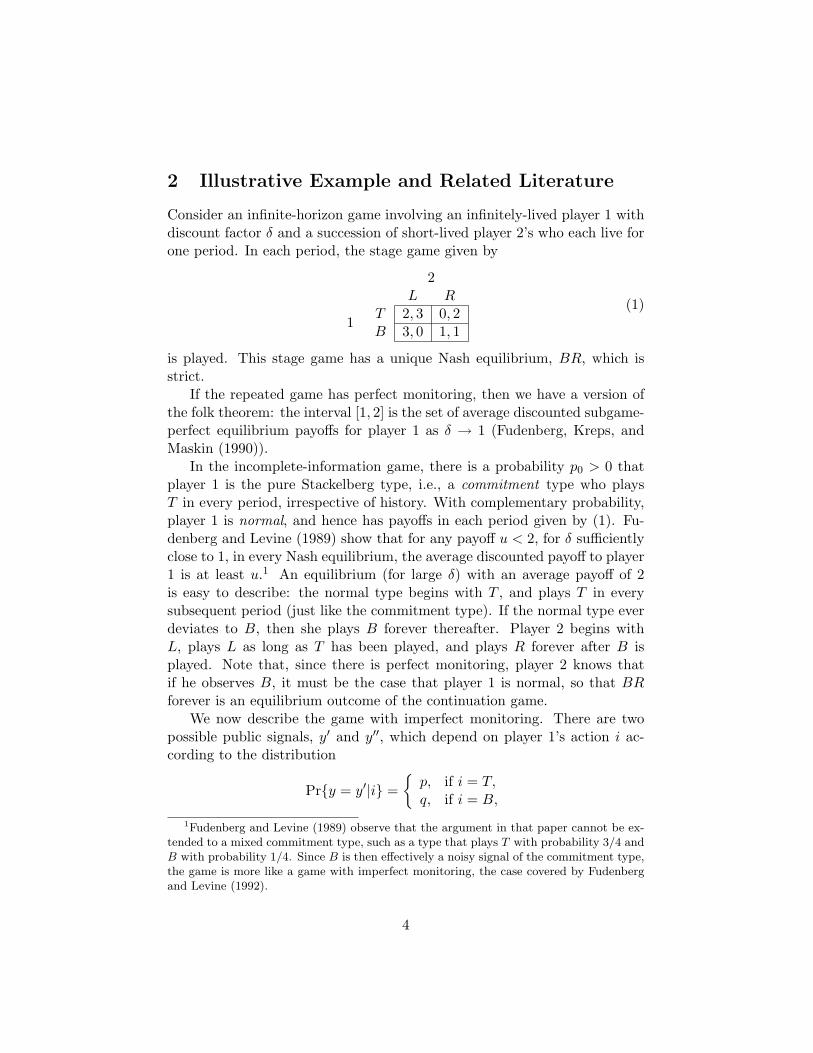
2 Illustrative Example and Related Literature
Consider an infinite-horizon game involving an infinitely-lived player 1 withdiscount factor δ and a succession of short-lived player 2’s who each live forone period. In each period, the stage game given by
1
2L R
T 2, 3 0, 2B 3, 0 1, 1
(1)
is played. This stage game has a unique Nash equilibrium, BR, which isstrict.
If the repeated game has perfect monitoring, then we have a version ofthe folk theorem: the interval [1, 2] is the set of average discounted subgame-perfect equilibrium payoffs for player 1 as δ → 1 (Fudenberg, Kreps, andMaskin (1990)).
In the incomplete-information game, there is a probability p0 > 0 thatplayer 1 is the pure Stackelberg type, i.e., a commitment type who playsT in every period, irrespective of history. With complementary probability,player 1 is normal, and hence has payoffs in each period given by (1). Fu-denberg and Levine (1989) show that for any payoff u < 2, for δ sufficientlyclose to 1, in every Nash equilibrium, the average discounted payoff to player1 is at least u.1 An equilibrium (for large δ) with an average payoff of 2is easy to describe: the normal type begins with T , and plays T in everysubsequent period (just like the commitment type). If the normal type everdeviates to B, then she plays B forever thereafter. Player 2 begins withL, plays L as long as T has been played, and plays R forever after B isplayed. Note that, since there is perfect monitoring, player 2 knows thatif he observes B, it must be the case that player 1 is normal, so that BRforever is an equilibrium outcome of the continuation game.
We now describe the game with imperfect monitoring. There are twopossible public signals, y′ and y′′, which depend on player 1’s action i ac-cording to the distribution
Pry = y′|i =p, if i = T,q, if i = B,
1Fudenberg and Levine (1989) observe that the argument in that paper cannot be ex-tended to a mixed commitment type, such as a type that plays T with probability 3/4 andB with probability 1/4. Since B is then effectively a noisy signal of the commitment type,the game is more like a game with imperfect monitoring, the case covered by Fudenbergand Levine (1992).
4

where p > q. Player 2’s actions are public. Player 1’s payoffs are as inthe above stage game (1), and player 2’s ex post payoffs are given in thefollowing matrix,
L R
y′ 3 (1− q) /(p− q) −3q/(p− q)
y′′ (p− 1)/(p− q) p/(p− q).
The ex ante payoffs for player 2 are thus still given by (1). This structureof ex post payoffs ensures that the information content of the public signaland player 2’s payoffs is the same.
This game is an example of what Fudenberg and Levine (1994) call amoral hazard mixing game. Even for large δ, the long-run player’s max-imum Nash (or, equivalently, sequential) equilibrium payoff is lower thanwhen monitoring is perfect (Fudenberg and Levine (1994, Theorem 6.1, part(iii))).2 For our example, it is straightforward to apply the methodology ofAbreu, Pearce, and Stacchetti (1990) to show that if 2p > 1 + 2q, then theset of Nash equilibrium payoffs for large δ is given by the interval[
1, 2− (1− p)(p− q)
]. (2)
There is a continuum of particularly simple equilibria, with player 1 ran-domizing in every period, with equal probability on T and on B, irrespectiveof history and player 2’s strategy having one period memory. After the sig-nal y′, player 2 plays L with probability α′ and R with probability 1 − α′.After y′′, player 2 plays L with probability α′′ and R with probability 1−α′′,with
2δ (p− q)(α′ − α′′
)= 1.
The maximum payoff of 2 − (1− p) / (p− q) is obtained by setting α′ = 1and
α′′ = 1− 12δ (p− q)
.
As in the case of perfect monitoring, we introduce incomplete informationby assuming there is a probability p0 > 0 that player 1 is the Stackelberg typewho plays T in every period. Fudenberg and Levine (1992) show that in thiscase as well, for any payoff u < 2, there is δ sufficiently close to 1 such that
2In other words, the folk theorem of Fudenberg, Levine, and Maskin (1994) does nothold when there are short-lived players.
5
in every Nash equilibrium, the expected average discounted payoff to player1 is at least u. We emphasize that u can exceed the upper bound in (2).Establishing that u is a lower bound on equilibrium payoffs is significantlycomplicated by the imperfect monitoring. Player 2 no longer observes theaction choices of player 1, and so any attempt by player 1 to manipulate thebeliefs of player 2 must be mediated through the full support signals. Theexplicit construction of equilibria in this case is also very difficult.
In this example, player 2’s posterior belief that player 1 is the Stackelbergtype is independent of 2’s actions and hence public information. As such theexample falls within the coverage of our Theorem 1. To develop intuition,temporarily restrict attention to Markov perfect equilibrium, with player2’s belief that player 1 is the Stackelberg type (i.e., player 1’s “reputation”)being the natural state variable. In any such equilibrium, the normal typecannot play T for sure in any period: if she did, the posterior after any signalin that period is the prior, and continuation play is also independent of thesignal. But then player 1 has no incentive to play T . Thus, in any period ofa Markov perfect equilibrium, player 1 must put positive probability on B.Consequently, the signals are informative, and so almost surely, when player1 is normal, beliefs must converge to zero probability on the Stackelbergtype.3
Our analysis is complicated by the fact that we do not restrict attentionto Markov perfect equilibria, as well as the possibility of more complicatedcommitment types than the pure Stackelberg type (for example, we allowfor nonstationary history-dependent mixing). In particular, uninformativesignals may have future ramifications.
While some of our arguments and results are reminiscent of the recentliterature on rational learning and merging, there are also important dif-ferences. For example, Jordan (1991) studies the asymptotic behavior of“Bayesian Strategy Processes,” in which myopic players play a Bayes-Nashequilibrium of the one-shot game in each period, players initially do not knowthe payoffs of their opponents, and players observe past play. The centralresult is that play converges to a one-shot Nash equilibrium of the complete-information game. In contrast, the player with private information in ourgame is long-lived and potentially very patient, introducing intertemporalconsiderations that do not appear in Jordan’s model, and the informationprocessing in our model is complicated by the imperfect monitoring.
3Benabou and Laroque (1992) study the Markov perfect equilibrium of a game withsimilar properties. They show that player 1 eventually reveals her type in any Markovperfect equilibrium.
6

A key idea in our results (in particular, Lemmas 2 and 5) is that ifsignals are statistically informative about a player’s behavior, then there islittle asymptotic value to other players learning private information that hasa nontrivial asymptotic impact on the first player’s behavior. Similar ideasplay an important role in merging arguments, which provide conditions un-der which a true stochastic process and beliefs over that process converge.Sorin (1999), for example, unifies much of the existing reputation literatureas well as recent results on repeated games with incomplete informationusing merging. Kalai and Lehrer (1995), again using merging, provide asimple argument that in reputation games, asymptotic continuation play isa subjective correlated equilibrium of the complete-information game (thatresult is immediate in our context, since we begin with a Nash equilibrium ofthe incomplete-information game, while it is a harder for Kalai and Lehrer(1995) since their hypothesis is a weaker). Subjective correlated equilibriumis a significantly weaker solution concept than objective correlated equi-librium. We discuss the relationship in Section 4.3, where we show thatasymptotic continuation play is an objective correlated equilibrium of thecomplete-information game.
The idea that reputations are temporary is a central theme of Jacksonand Kalai (1999), who are interested in reputation in finitely repeated nor-mal form games (for which Fudenberg and Maskin (1986) prove a reputationfolk theorem). Jackson and Kalai (1999) prove that if the finitely repeatednormal-form game is itself repeated (call the finite repetition of the originalstage a round), with new players (although not a new draw from a rich setof types) in each round, then eventually, reputations cannot affect play inthe finitely repeated game. While the conclusion looks the same as ours, themodel is quite different. In particular, players in one round of the finitelyrepeated game do not internalize the effects of their behavior on beliefs andso behavior of players in future rounds. Moreover, there is perfect moni-toring of actions in each stage game. We exploit the imperfection of themonitoring to show that reputations are eventually dissipated even whenplayers recognize their long-run incentives to preserve these reputations.
3 The Model
3.1 The Complete-Information Game
The stage game is a two-player simultaneous-move finite game of publicmonitoring. Player 1 chooses an action i ∈ 1, 2, ..., I ≡ I and player 2simultaneously chooses an action j ∈ 1, 2, ..., J ≡ J . The public signal,
7
denoted y, is drawn from a finite set, Y . The probability that y is realizedunder the action profile (i, j) is given by ρy
ij . The ex post stage-game payoffto player 1 (respectively, 2) from the action i (resp., j) and signal y is givenby f1(i, y) (resp., f2(j, y)). The ex ante stage game payoffs are π1 (i, j) =∑
y f1 (i, y) ρyij and π2 (i, j) =
∑y f2 (j, y) ρy
ij .The stage game is infinitely repeated. Player 1 (“she”) is a long-lived
(equivalently, long-run) player with discount factor δ < 1; her payoffs in theinfinite horizon game are the average discounted sum of stage-game payoffs,(1− δ)
∑∞t=0 δ
tπ1(it, jt). The role of player 2 (“he”) is played by a sequenceof short-lived (or short-run) players, each of whom only plays once.
Players only observe the realizations of the public signal and their ownpast actions (the period-t player 2 knows the action choices of the previ-ous player 2’s). Player 1 in period t has a private history, consisting of thepublic signals and her own past actions, denoted by h1t ≡ ((i0, y0), (i1, y1),. . . , (it−1, yt−1)) ∈ H1t ≡ (I × Y )t. Similarly, a private history for player 2is denoted h2t ≡ ((j0, y0), (j1, y1), . . . , (jt−1, yt−1)) ∈ H2t ≡ (J × Y )t. LetH`t∞t=0 denote the filtration on (I × J × Y )∞ induced by the private his-tories of player ` = 1, 2. The public history observed by both players is thesequence (y0, y1, ..., yt−1) ∈ Y t. Let Ht∞t=0 denote the filtration inducedby the public histories.
We assume the public signals have full support (Assumption 1), so everysignal y is possible after any action profile. We describe circumstances un-der which this assumption can be weakened in Section 4.1. We also assumethat with sufficient observations player 2 can correctly identify, from the fre-quencies of the signals, any fixed stage-game action of player 1 (Assumption2).
Assumption 1 (Full Support) ρyij > 0 for all (i, j) ∈ I × J and y ∈ Y .
Assumption 2 (Identification) For all j ∈ J , there are I linearly inde-pendent columns in the matrix (ρy
ij)y∈Y,i∈I .
A behavior strategy for player 1 is a map σ1 : ∪∞t=0H1t → ∆I , fromthe set of private histories of lengths t = 0, 1, . . . to the set of distributionsover current actions. Similarly, a behavior strategy for player 2 is a mapσ2 : ∪∞t=0H2t → ∆J .
A strategy profile σ = (σ1, σ2) induces a probability distribution P σ over(I × J × Y )∞. Let Eσ[·|H`t] denote player `’s expectations with respect tothis distribution conditional on H`t.4
4This expectation is well-defined, since I, J , and Y are finite.
8

In equilibrium, the short-run player plays a best response after everyequilibrium history. Player 2’s strategy σ2 is a best response to σ1 if, for allt,5
Eσ[ π2(it, jt) | H2t] ≥ Eσ[ π2(it, j) | H2t], ∀j ∈ J P σ-a.s.
Denote the set of such best responses by BR(σ1).The definition of a Nash equilibrium is completed by the requirement
that player 1’s strategy maximizes her expected utility:
Definition 1 A Nash equilibrium of the complete-information game is astrategy profile σ∗ = (σ∗1, σ
∗2) with σ∗2 ∈ BR(σ∗1) such that for all σ1:
Eσ∗
[(1− δ)
∞∑s=0
δsπ1(is, js)
]≥ E(σ1,σ∗2)
[(1− δ)
∞∑s=0
δsπ1(is, js)
].
This requires that after any history that can arise with positive probabilityunder the equilibrium profile, player 1’s strategy maximize her continuationexpected utility. Hence, if σ∗ is a Nash equilibrium, then for all σ1 and forall t, P σ∗-almost surely
Eσ∗
[(1− δ)
∞∑s=t
δs−tπ1(is, js)
∣∣∣∣∣H1t
]≥ E(σ1,σ∗2)
[(1− δ)
∞∑s=t
δs−tπ1(is, js)
∣∣∣∣∣H1t
].
Since every public history occurs with positive probability, the outcomeof any Nash equilibrium is a perfect Bayesian equilibrium outcome.
3.2 Never an Equilibrium Strategy in the Long Run
Suppose (σ1, σ2) is an equilibrium of the complete-information game andthat we extend this to an incomplete-information game by introducing thepossibility of a commitment type who plays σ1. The profile in which player1 always plays like the commitment type and player 2 follows σ2 is then anequilibrium of the incomplete-information game. Moreover, player 2 learnsnothing about the type of player 1 in this equilibrium. Hence, player 1 canmaintain a permanent reputation for behavior that would be an equilibriumwithout that reputation, i.e., in the complete-information game.
5Note that j, the action of player 2, on the right hand side of the inequality is notrandom, and so the right expectation is being taken only with respect to it, the choice ofplayer 1.
9
More generally, there may be no difficulty in maintaining a reputation forbehavior that features nonequilibrium play in the first ten periods and there-after switches to σ1. Questions of whether player 2 will learn player 1’s typecan only be settled by long-run characteristics of strategies, independent ofinitial histories. We accordingly introduce the concept of a strategy’s beingnever an equilibrium strategy in the long run. Such a strategy for player1 has the property that for all best responses by player 2 and all historiesh1t, there is always a profitable deviation for player 1 in periods beyondsome sufficiently large T . We emphasize that in the following definition, theBR (σ1) is the set of player 2 best responses in the complete-informationgame.
Definition 2 The strategy σ1 is never an equilibrium strategy in the longrun, if there exists T and ε > 0 such that, for every σ2 ∈ BR(σ1) and forevery t ≥ T , there exists σ1 such that P σ-a.s,
Eσ
[(1− δ)
∞∑s=t
δs−tπ1(is, js)
∣∣∣∣∣H1t
]+ε < E(σ1,σ2)
[(1− δ)
∞∑s=t
δs−tπ1(is, js)
∣∣∣∣∣H1t
].
It is possible for a strategy to never be an equilibrium strategy in thelong run for some discount factors, but not for others.
This definition is most easily interpreted when the strategy is eithersimple or implementable by a finite automaton:
Definition 3 (1) A behavior strategy σ1 is public if it is measurable withrespect to Ht, so that the mixture over actions induced in each perioddepends only upon the public history.
(2) A behavior strategy σ1 is simple if it is a constant function, i.e.,induces the same (possibly degenerate) mixture over ∆I after every history.
(3) A public strategy σ1 is implementable by a finite automaton if thereexists a finite set W , an action function d : W → ∆I , a transition functionϕ : W × Y → W , and an initial element w0 ∈ W , such that σ1 (ht) =d (w (ht)), where w (ht) is the state reached from w0 under the public historyht and transition rule ϕ.
Any pure strategy is realization equivalent to a public strategy. A simplestrategy is clearly public and is implementable by a finite automaton witha single state.
The following Lemma shows that for simple strategies or strategies im-plementable by a finite automata, being never an equilibrium in the long run
10

is essentially equivalent to not being part of a Nash equilibrium of the stagegame or the complete-information repeated game. The point of Definition2 is to extend this concept to strategies that have transient initial phases orthat never exhibit a stationary structure.
Lemma 1 Assume the monitoring has full support (Assumption 1).
1.1 Suppose player 2 has a unique best reply to some mixture ς ∈ ∆I .The simple strategy of always playing ς is never an equilibrium strat-egy in the long run if and only if ς is not part of a stage-game Nashequilibrium.
1.2 Suppose σ1 is a public strategy implementable by the finite automaton(W,d, ϕ,w0), with every state in W reachable from every other state inW under ϕ. If player 2 has a unique best reply to d (w) for all w ∈W ,then σ1 is never an equilibrium strategy in the long run if and only ifσ1 is not part of a Nash equilibrium of the complete-information game.
Proof. We prove only part 2, since part 1 is similar (but easier). Theonly if direction is obvious. So, suppose σ1 is not a Nash equilibrium of thecomplete-information game. Since player 2 always has a unique best reply tod (w), σ2 is public, and can also be represented as a finite state automaton,with the same set of states and transition function as σ1. Since σ1 is nota Nash equilibrium, there is some state w′ ∈ W , and some action i′ not inthe support of d (w′) such that when the state is w′, playing i′ and thenfollowing σ1 yields a payoff that is strictly higher than following σ1 at w′.Since the probability of reaching w′ from any other state is strictly positive(and so bounded away from zero), σ1 is never an equilibrium in the longrun.
The example from Section 2 illustrates the necessity of the condition inLemma 1 that player 2 have a unique best response. The simple strategythat places equal probability on T and B is part of many equilibria of thecomplete-information game (as long as δ > 1/ [2 (p− q)]), and hence fails thecriterion for being never an equilibrium strategy in the long run. However,this strategy is not part of an equilibrium of the stage game, in contrast toLemma 1.1. On the other hand, player 2 has a unique best response to anymixture in which player 1 randomizes with probability of T strictly largerthan 1
2 , and a simple strategy that always plays such a mixture is not partof a stage-game equilibrium and is never an equilibrium strategy in the longrun.
11
If we were only interested in the presence of “Stackelberg” commitmenttypes, and the attendant lower bounds on player 1’s ex ante payoffs, it wouldsuffice to consider commitment types who follow simple strategies. However,allowing more general types leaves the structure of the argument unaffectedwhile simplifying our discussion of the case where player 2 is also long-lived(see Section 8).
3.3 The Incomplete-Information Game
We now formally describe the game with incomplete information about thetype of player 1. For expositional clarity only, much of our analysis focuseson the case of one commitment type. Section 7 discusses the case of manycommitment types.
At time t = −1 a type of player 1 is selected. With probability 1 − p0
she is the “normal” type, denoted n, with the preferences described above.With probability p0 > 0 she is a “commitment” type, denoted c, who playsa fixed, repeated-game strategy σ1.
A state of the world is now a type for player 1 and sequence of actionsand signals. The set of states is then Ω = n, c× (I × J × Y )∞. The priorp0, commitment strategy σ1 and the strategy profile of the normal playersσ = (σ1, σ2) induce a probability measure P over Ω, which describes how anuninformed player expects play to evolve. The strategy profile σ = (σ1, σ2)(respectively σ) determines a probability measure P (respectively P ) over Ω,which describes how play evolves when player 1 is the commitment (respec-tively normal) type. Since P and P are absolutely continuous with respectto P , any statement that holds P -almost surely, also holds P - and P -almostsurely. Henceforth, we will use E[·] to denote unconditional expectationstaken with respect to the measure P . E[·] and E[·] are used to denote con-ditional expectations taken with respect to the measures P and P . Genericoutcomes are denoted by ω. The filtrations H1t∞t=0, H2t∞t=0, and Ht∞t=0
on (I × J × Y )∞ can also be viewed as filtrations on Ω in the obvious way;we use the same notation for these filtrations (the relevant sample space willbe obvious). As usual, denote by H`∞ the σ-algebra generated by ∪∞t=0H`t.
For any repeated-game behavior strategy σ1 : ∪∞t=0H1t → ∆I , denoteby σ1t the tth period behavior strategy, so that σ1 can be viewed as thesequence of functions (σ10, σ11, σ12, . . .) with σ1t : H1t → ∆I . We extendσ1t from H1t to Ω in the obvious way , so that σ1t (ω) ≡ σ1t(h1t(ω)), whereh1t(ω) is player 1’s t-period history under ω. A similar comment applies toσ2.
Given the strategy σ2, the normal type has the same objective func-
12
tion as in the complete-information game. Player 2, on the other hand, ismaximizing E[ π2(it, j) | H2t], so that after any history h2t, he is updatinghis beliefs over the type of player 1 that he is facing.6 The profile (σ1, σ2)is a Nash equilibrium of the incomplete-information game if each player isplaying a best response.
At any equilibrium, player 2’s posterior belief in period t that player1 is the commitment type is given by the H2t-measurable random variablept : Ω → [0, 1]. By Assumption 1, Bayes’ rule determines this posterior afterall sequences of signals. Thus, in period t, player 2 is maximizing
ptE[ π2(it, j) | H2t] + (1− pt) E[ π2(it, j) | H2t]
P -almost surely. At any Nash equilibrium of this game, the belief pt is abounded martingale with respect to the filtration H2tt and measure P .7
It therefore converges P -almost surely (and hence P - and P -almost surely)to a random variable p∞ defined on Ω. Furthermore, at any equilibrium theposterior pt is a P -submartingale and a P -supermartingale with respect tothe filtration H2t.
A final word on notation: The expression E [σ1t|H2s] is the standardconditional expectation, viewed as a H2s measurable random variable on Ω,while E [σ1 (h1t) |h2s] is the conditional expected value of σ1 (h1t) (with h1t
viewed as a random history) conditional on the observation of the historyh2s.
4 Impermanent Reputations
Consider an incomplete-information game, with a commitment type strat-egy that is never an equilibrium strategy in the long run. Suppose thereis a Nash equilibrium in which both the normal and the commitment typereceive positive probability in the limit (on a positive probability set of his-tories). On this set of histories, player 2 cannot distinguish between signalsgenerated by the two types (otherwise player 2 can ascertain which type heis facing), and hence must believe, on this set of histories, that the normaland commitment types are playing the same strategies on average. But thenplayer 2 must eventually, again on the same set of histories, best reply tothe average behavior of the commitment type. Since the commitment type’s
6As in footnote 5, j is not random and the expectation is being taken with respect toit, the action choice of player 1.
7These properties are well-known. Proofs for the model with perfect monitoring (whichcarry over to imperfect monitoring) can be found in Cripps and Thomas (1995).
13
behavior is never an equilibrium strategy in the long run, player 1 does notfind it optimal to play the commitment-type strategy in response to 2’s bestresponse, leading us very close to a contradiction.
There are two difficulties in making this argument precise. First, sincethe game has imperfect monitoring, player 2 has imperfect knowledge ofplayer 1’s private history and thus the continuation strategy of player 1. Ifthe commitment type strategy is not pure, it may be that the normal typeis following a private strategy that on average is like the public commitmentstrategy, but which is different from the latter on every history. Second, theset of histories upon which the argument proceeded is typically not knownby either player at any point (although it will be in H2∞). Consequently,player 1 may never know that player 2 is best responding to the averageplay of the commitment type.
These two difficulties interact. Our first and easier result (Theorem 1) isfor the case where the informativeness of the signal about player 1’s actionis independent of player 2’s action. In this case, in any equilibrium, player2’s beliefs about the type of player 1 are public and so the second difficultydoes not arise. We can then surmount the first difficulty to show thatreputations are impermanent, even when the commitment type is followinga mixed public strategy.
The second, harder result (Theorem 2) is for the case where the informa-tiveness of the signal about player 1’s action depends on player 2’s action.This case is important because, as we describe in Section 6, it also coversgames with private monitoring. In this case, we can only show that reputa-tions are impermanent when we remove the first difficulty by imposing thestronger requirement that the commitment type is following a pure (thoughnot necessarily simple or finitely-implementable) strategy.
Theorem 1 is presented in the next subsection with its proof given inSection 5.2, Theorem 2 is presented in Section 4.2 and proved in Section5.3. (Some preliminaries are presented in Section 5.1.) The behavioralimplications of the theorems are discussed in Sections 4.3 and 4.4.
4.1 The “Easy” Case: Player 2’s Beliefs Known
In the “easy” case, player 2’s beliefs about player 1 are known by player 1.The full support assumption (Assumption 1) implies that player 1 in
general does not know the action choice of player 2. Under the followingassumption, however, player 1 can calculate 2’s inference without knowing2’s action:
14
Assumption 3 (Independence) For any (possibly mixed) actions ζ1 ∈∆I , signal y ∈ Y , and actions i, j, and j′,
Pri|y, j, ζ1 = Pri|y, j′, ζ1,
where Pri|y, j, ζ1 is the posterior probability of player 1 having chosenpure action i, given mixed action ζ1 and given that player 2 observed signaly after playing action j.
Theorem 1 Suppose ρ satisfies Assumptions 1, 2, and 3. Suppose σ1 is apublic strategy with finite range that is never an equilibrium strategy in thelong run. Then in any Nash equilibrium, pt → 0 P -almost surely.
The definition of never an equilibrium in the long run requires player 1’speriod-t deviation to generate an expected payoff increase, conditional onreaching period t, of at least ε. Our proof rests on the argument that if play-ers are eventually almost certain that the normal type player 1 is behavinglike a commitment type that is never an equilibrium in the long run, thenthe normal type will have a profitable deviation. Without the ε wedge inthis definition, it is conceivable that while players become increasingly cer-tain that the normal type is playing like the commitment type, the payoffpremium to deviating from the nonequilibrium commitment-type strategydeclines sufficiently rapidly as to ensure that the players are never certainenough to support a deviation. The ε-uniform bound on the profitability ofa deviation precludes this possibility.
Section 5.1.2 explains how the assumptions that σ has a finite rangeplays a role similar to that of the ε just described. The requirement thatσ1 be public ensures that whenever player 2 is convinced that player 1 isplaying like the commitment type, player 2 can identify the period-t strategyrealization σ1(h1t) and play a best response.
A sufficient condition for Assumption 3 is that the public signal y be avector (y1, y2) ∈ Y1 × Y2 = Y , with y1 a signal of player 1’s action and y2
an independent signal of player 2’s action. In this case, action i induces aprobability distribution ρi over Y1 while action j induces ρj over Y2, with
ρyij = ρy1
i ρy2j ∀i, j, y. (3)
The full-support Assumption 1 can be relaxed if (3) holds. The keyingredient in the proof of Theorem 1 is that players 1 and 2 are symmetricallyinformed about 2’s beliefs, and that the signal not reveal player 1’s action (so
15

that trigger profiles are not equilibria). Assumption 1 can thus be replacedby the requirement that, for all i and y1 ∈ Y1,
ρy1i > 0.
Assumption 2, in the presence of (3), is equivalent to the requirement thatthere are I linearly independent columns in the matrix
(ρy1i )y1∈Y1,i∈I .
Since the key implication of Assumption 3 is that player 1 knows player2’s posterior belief, an alternative to Assumption 3 is to assume that player2’s actions are public, while maintaining imperfect public monitoring ofplayer 1’s actions. In this case, Y = Y1 × J , where Y1 is the set of publicsignals of player 1’s actions, and
ρ(y1,j′)ij = 0 (4)
for all i ∈ I, j 6= j′ ∈ J , and y1 ∈ Y . The public nature of player 2’s actionsimplies that H2t = Ht, and hence pt is measurable with respect to Ht (andso player 1 knows the posterior of belief of player 2).
When player 2’s actions are public, the full support assumption is
ρ(y1,j)ij > 0
for all (i, j) ∈ I × J and y1 ∈ Y1, while the identification assumption is nowthat for all j ∈ J , there are I linearly independent columns in the matrix(
ρ(y1,j)ij
)y1∈Y1,i∈I
.
4.2 The Harder Case: Player 2’s Beliefs Unknown
The harder case is where player 2’s beliefs about player 1 are not known byplayer 1. Our method of proof requires that player 1 can draw inferencesabout player 2’s actions, and the following assumption allows this:
Assumption 4 For all i ∈ I, there are J linearly independent columns inthe matrix (ρy
ij)y∈Y,j∈J .
This assumption is dramatically weaker than Assumption 3. Considerthe example of Section 2, except that player 2’s choice of L or R is private.Let ρ′ij be the probability of the signal y′ under the action profile ij ∈
16
T,B × L,R, so that the probability of the signal y′′ is given by 1− ρ′ij .Assumption 2 requires ρ′TL 6= ρ′BL and ρ′TR 6= ρ′BR, while Assumption 4requires ρ′TL 6= ρ′TR and ρ′BL 6= ρ′BR. The assumptions are satisfied ifρ′TL > ρ′BL and ρ′TR < ρ′BR, so that y′ is a signal that player 1 has playedT if player 2 had played L, but is a signal that she had played B if 2 hadplayed R. Unless player 1 knows the action of player 2, she will not knowhow the signal is interpreted.
As we discussed at the beginning of this section, the cost of weakeningAssumption 3 to Assumption 4 is that we must assume the commitment typedoes not randomize. The commitment type’s strategy, while pure, can stilldepend upon histories in arbitrarily complicated ways. We also emphasizethat we are not imposing any restrictions on the normal type’s behavior(other than it be a best response to the behavior of the short-lived players).
Theorem 2 Suppose ρ satisfies Assumptions 1, 2, and 4. Suppose σ1 is apure strategy that is never an equilibrium strategy in the long run. Then inany Nash equilibrium, pt → 0 P -almost surely.
Since any pure strategy is realization equivalent to a public strategy,it is again the case that whenever player 2 is convinced that player 1 isplaying like the commitment type, player 2 can identify the period-t strategyrealization σ1(h1t) and play a best response.
4.3 Asymptotic Equilibrium Play
We now explore the implications for equilibrium play of the impermanenceof reputations. More precisely, we will show that in the limit, the normaltype of player 1 and player 2 play a correlated equilibrium of the complete-information game. Hence, differences in the players’ subjective beliefs abouthow play will continue vanish in the limit. This strengthens the result onconvergence to subjective equilibria (see below) obtained by Kalai and Lehrer(1995, Corollary 4.4.1). To begin, we describe some notation for the corre-lated equilibrium of our repeated games with imperfect monitoring.
We use the term continuation game for the game with initial period inperiod t, ignoring the period t-histories.8 We use the notation t′ = 0, 1, 2, ...for a period of play in a continuation game (which may be the original game)
8Since a strategy profile of the original game induces a probability distribution overt-period histories, H1t ×H2t, we can view the period t continuation, together with a typespace H1t×H2t and induced distribution on that type space, as a Bayesian game. Differentstrategy profiles in the original game induce different distributions over the type space inthe continuation game.
17

and t for the time elapsed prior to the start of the continuation game. Apure strategy for player 1, s1, is a sequence of maps s1t′ : H1t′ → I fort′ = 0, 1, . . ..9 Thus, s1t′ ∈ IH1t′ and s1 ∈ I∪t′H1t′ ≡ S1, and similarly s2 ∈S2 ≡ J∪t′H2t′ . The spaces S1 and S2 are countable products of finite sets.We equip the product space S ≡ S1 × S2 with the σ-algebra generated bythe cylinder sets, denoted by S. Denote the players’ payoffs in the infinitelyrepeated game (as a function of these pure strategies) as follows
u1(s1, s2) ≡ E[(1− δ)∞∑
t′=0
δt′π1(it′ , jt′)]
ut′2 (s1, s2) ≡ E[π2(it′ , jt′)].
The expectation above is taken over the action pairs (it′ , jt′). These arerandom, given the pure strategy profile (s1, s2), because the pure actionplayed in period t depends upon the random public signals.
In the following definitions, we follow Hart and Schmeidler (1989) inusing the ex ante definition of correlated equilibria for infinite pure strategysets. Note also that we need player 2’s incentive compatibility conditions tohold at all times t′, because of player 2’s zero discounting.
Definition 4 A subjective correlated equilibrium of the complete-informationgame is a pair of measures µ`, ` = 1, 2, on (S,S) such that for all S-measurable functions ζ1 : S1 → S1, ζ2 : S2 → S2∫
S[u1(s1, s2)− u1(ζ1(s1), s2)]dµ1 ≥ 0; (5)∫
S[ut′
2 (s1, s2)− ut′2 (s1, ζ2(s2))]dµ2 ≥ 0, ∀t′. (6)
A correlated equilibrium of the complete-information game is a subjectivecorrelated equilibrium satisfying µ1 = µ2.
Let M denote the space of probability measures µ on (S,S), equippedwith the product topology. Then, a sequence µn converges to µ if, for eachτ > 0, we have
µn|I(I×Y )τ×J(J×Y )τ → µ|I(I×Y )τ×J(J×Y )τ . (7)
Moreover, M is sequentially compact with this topology. Payoffs for players1 and 2 are extended to M in the obvious way. Since player 1’s payoffs are
9Note that we have used σ1 for general behavior strategies, not only pure strategies.
18
discounted, the product topology is strong enough to guarantee continuityof u1 : M→R. Each player 2’s payoff is trivially continuous. The set ofmixed strategies for player ` is denoted by M`.
Fix an equilibrium of the incomplete-information game with imperfectmonitoring. When player 1 is the normal (respectively, commitment) type,the monitoring technology and the behavior strategies (σ1, σ2) (resp., (σ1, σ2))induce a probability measure φt (resp., φt) on the t-period histories (h1t, h2t) ∈H1t×H2t. If the normal type of player 1 observes a private history h1t ∈ H1t,her strategy σ1, specifies a behavior strategy in the continuation game. Thisbehavior strategy is realization equivalent to a mixed strategy λ
h1t ∈M1 forthe continuation game. Similarly, the commitment type will play a mixedstrategy λ
h1t ∈ M1 for the continuation game and player 2 will form hisposterior pt(h2t) and play the mixed strategy λh2t ∈M2 in the continuationgame. Conditional on player 1 being normal, the composition of the prob-ability measure φt and the measures (λ
h1t, λh2t) induces a joint probability
measure, ρt, on the pure strategies in the continuation game and player 2’sposterior (the space S × [0, 1]). Similarly, conditional upon player 1 beingthe commitment type, there is a measure ρt on S × [0, 1]. Let µt denote themarginal of ρt on S and µt denote the marginal of ρt on S.
At the fixed equilibrium, the normal type is playing in an optimal wayfrom time t onwards given her available information. This implies that forall S-measurable functions ζ1 : S1 → S1,∫
Su1(s1, s2)dµt ≥
∫Su1(ζ1(s1), s2)dµt. (8)
Let S × B denote the product σ-algebra on S × [0, 1] generated by S on Sand the Borel σ-algebra on [0, 1]. Player 2 is also playing optimally fromtime t onwards, which implies that for all S × B-measurable functions ξ2 :S2 × [0, 1] → S2, and for all t′,∫
S×[0,1]ut′
2 (s1, s2)d(p0ρt+(1−p0)ρt) ≥∫
S×[0,1]ut′
2 (s1, ξ2(s2, pt))d(p0ρt+(1−p0)ρt).
Comparing the previous two inequalities with (5) and (6), it is clear thatthe equilibrium behavior from period t onwards is a subjective correlatedequilibrium for the continuation game for all t.
If we had metrized M, a natural formalization of the idea that asymp-totically, the normal type and player 2 are playing a correlated equilibriumis that the distance between the set of correlated equilibria and the induceddistributions µt on S goes to zero. While M is metrizable, a simpler and
19
equivalent formulation is that the limit of every convergent subsequence ofµt is a correlated equilibrium. This equivalence is an implication of thesequential compactness of M, since every subsequence of µt has a conver-gent sub-subsequence. The proof is in Section A.1.
Theorem 3 Fix a Nash equilibrium of the incomplete-information gameand suppose pt → 0 P -almost surely. Let µt denote the distribution on Sinduced in period t by the Nash equilibrium. The limit of every convergentsubsequence is a correlated equilibrium of the complete-information game.
Since players have access to a coordination device, namely histories,in general it is not true that Nash equilibrium play of the incomplete-information game eventually looks like Nash equilibrium play of the complete-information game.
Suppose the Stackelberg payoff is not a correlated equilibrium payoff ofthe complete-information game. Recall that Fudenberg and Levine (1992)provide a lower bound on equilibrium payoffs in the incomplete-informationgame of the following type: Fix the prior probability of the Stackelberg(commitment) type. Then, there is a value for the discount factor, δ, suchthat if δ > δ, then in every Nash equilibrium, the long-lived player’s ex antepayoff is essentially no less than the Stackelberg payoff. The reconciliation ofthis result with Theorem 3 lies in the order of quantifiers: while Fudenbergand Levine (1992) fix the prior, p0, and then select δ (p0) large (with δ (p0) →1 as p0 → 0), we fix δ and examine asymptotic play, so that eventually pt issufficiently small that δ (pt) > δ.
We do not know if Nash equilibrium play in the incomplete-informationgame eventually looks like a public randomization over Nash equilibriumplay in the complete-information game.10
4.4 Impermanent Restrictions on Behavior
We now provide a partial converse to the previous section by identifying aclass of equilibria of the complete-information game to which equilibriumplay of the incomplete-information game can converge. The constructionof equilibria in incomplete-information games is difficult, and so we restrict
10As far as we know, it is also not known whether the result of Fudenberg and Levine(1994, Theorem 6.1, part (iii)) extends to correlated equilibrium. That is, for moral hazardmixing games and for large δ, is it true that the long-run player’s maximum correlatedequilibrium payoff is lower than when monitoring is perfect? We believe that, at least forsimple games like that described in Section 2, allowing for correlation does not increasethe long-lived player’s payoff.
20
attention to the case in which the posterior beliefs of player 2 are known byplayer 1.
Recall that in the example of Section 2, the stage game has a (unique)strict Nash equilibrium BR. Moreover, this achieves player 1’s minmaxutility. It is a straightforward implication of Fudenberg and Levine (1992)that the presence of the commitment type ensures that, as long as player 1is sufficiently patient, for much of the initial history of the game, in everyequilibrium, play is like TR. On the other hand, an implication of Theorem4 below, is that for the same parameters, (in particular, the same priorprobability of the commitment type), there is an equilibrium in which witharbitrarily high probability under P , BR is eventually played in every period.The construction of such an equilibrium must address the following twoissues. First, reputation effects may ensure that for a long period of time,equilibrium play will be very different from BR (this is just Fudenberg andLevine (1992)). Theorem 4 is consistent with this, since it only claims thatin the equilibrium of interest, BR is eventually played in every period withhigh probability. The second issue is that, even if reputation effects are notinitially operative (because the initial belief that player 1 is the commitmenttype is low relative to the discount factor), with positive probability (albeitsmall), a sequence of signals will arise that will make reputation effectsoperative (because the posterior that player 1 is the commitment type isincreased sufficiently).
Theorem 4 Suppose the assumptions of Theorem 1 are satisfied (i.e., ρsatisfies Assumptions 1, 2, and 3, and σ1 is a public strategy with finiterange that is never an equilibrium strategy in the long run). Suppose (i∗, j∗)is a strict Nash equilibrium of the stage game. Given any prior p0 and any δ,for all ε > 0, there exists a Nash equilibrium of the incomplete-informationgame in which the P -probability of the event that eventually (i∗, j∗) is playedin every period is at least 1− ε.
The proof is in Section A.2.
5 Proofs of Theorems 1 and 2
5.1 Preliminary results
5.1.1 Player 2’s Posterior Beliefs
The first step is to show that either player 2’s expectation (given his privatehistory) of the strategy played by the commitment type is in the limit iden-
21

tical to his expectation of the strategy played by the normal type, or player2’s posterior probability that player 1 is the commitment type converges tozero (given that player 1 is indeed normal). This is an extension of a familiarmerging-style argument to the case of imperfect monitoring. If, for a givenprivate history for player 2, the distributions generating his observations aredifferent for the normal and commitment types, then he will be updating hisposterior, continuing to do so as the posterior approaches zero. His posteriorconverges to something strictly positive only if the distributions generatingthese observations are in the limit identical for each private history. In thestatement of the following Lemma, h1t is to be interpreted as a functionfrom Ω to (I × Y )t.
Lemma 2 At any Nash equilibrium of a game satisfying Assumptions 1 and2,11
limt→∞
pt(1− pt)∥∥∥E[ σ1t | H2t ]− E[ σ1t | H2t ]
∥∥∥ = 0, P -a.s. (9)
Proof. Let pt+1(h2t; jt, yt) denote player 2’s belief in period t+ 1 afterplaying jt in period t, observing the signal yt in period t, and given thehistory h2t. By Bayes’ rule,
pt+1(h2t; jt, yt) =pt Pr[yt|h2t, jt, c]
pt Pr[yt|h2t, jt, c] + (1− pt) Pr[yt|h2t, jt, n].
The probability player 2 assigns to observing the signal yt from the commit-ment type is E[
∑i∈I σ
i1(h1t)ρ
yt
ijt|h2t], and from the normal type is E[
∑i∈I σ
i1(h1t)ρ
yt
ijt|h2t].
Using the linearity of the expectations operator, we write pt+1(h2t; jt, yt) as
pt+1(h2t; jt, yt) =pt
∑i∈I ρ
yt
ijtE[σi
1(h1t)|h2t]∑i∈I ρ
yt
ijt
(ptE[σi
1(h1t)|h2t] + (1− pt)E[σi1(h1t)|h2t]
) .Rearranging this formula allows us to write
pt(1− pt)∑i∈I
ρyt
ijt
(E[σi
1(h1t)|h2t]− E[σi1(h1t)|h2t]
)= (pt+1 − pt)
∑i∈I
ρyt
ijt
(ptE[σi
1(h1t)|h2t] + (1− pt)E[σi1(h1t)|h2t]
).
The summation on the right is bounded above by maxi ρyt
ijt< 1, thus
pt(1− pt)
∣∣∣∣∣∑i∈I
ρyt
ijt
(E[σi
1(h1t)|h2t]− E[σi1(h1t)|h2t]
)∣∣∣∣∣ ≤ |pt+1 − pt|.
11We use ‖x‖ to denote the sup-norm on Rn.
22

For any fixed realization y of the signal yt, it follows that for all h2t and jt,
pt(h2t)(1− pt(h2t))
∣∣∣∣∣∑i∈I
ρyijt
(E[σi
1(h1t)|h2t]− E[σi1(h1t)|h2t]
)∣∣∣∣∣≤ max
y′
∣∣pt+1(h2t; jt, y′)− pt(h2t)∣∣ . (10)
Since pt is a P -almost sure convergent sequence, it is Cauchy P -almostsurely.12 So the right hand side of (10) converges to zero P -almost surely.Thus, for any y,
pt(1− pt)
∣∣∣∣∣∑i∈I
ρyijt
(E[σi
1t|H2t]− E[σi1t|H2t]
)∣∣∣∣∣ → 0, P -a.s. . (11)
Hence, if both types are given positive probability in the limit then thefrequency that any signal is observed is identical under the two types.
We now show that (11) implies (9). Let Πjt be a |Y | × |I| matrix whosey-th row, for each signal y ∈ Y , contains the terms ρy
ijtfor i = 1, . . . , |I|.
Then as (11) holds for all y (and Y is finite), it can be restated as
pt(1− pt)∥∥∥Πjt
(E[σ1t|H2t]− E[σ1t|H2t]
)∥∥∥ → 0, P -a.s., (12)
where ‖.‖ is the supremum norm. By Assumption 2, the matrices Πjt haveI linearly independent columns for all jt, so x = 0 is the unique solutionto Πjtx = 0 in RI . In addition, there exists a strictly positive constantb = infj∈J,x 6=0 ‖Πjx‖/‖x‖. Hence ‖Πjx‖ ≥ b‖x‖ for all x ∈ RI and all j ∈ J .From (12), we then get
pt(1− pt)∥∥∥Πjt
(E[σ1t|H2t]− E[σ1t|H2t]
)∥∥∥≥ pt(1− pt)b
∥∥∥E[σ1t|H2t]− E[σ1t|H2t]∥∥∥ → 0, P -a.s.,
which implies (9).
Condition (9) says that either player 2’s best prediction of the normaltype’s behavior at the current stage is identical to his best prediction of thecommitment type’s behavior (that is, ‖ E[ σ1t | H2t ]− E[ σ1t | H2t ] ‖ → 0P -almost surely), or the type is revealed (that is, pt(1 − pt) → 0 P -almost
12Note that the analysis is now global, rather than local, in that we treat all the expres-sions as functions on Ω.
23

surely). However, lim pt < 1 P -almost surely, and hence (9) implies a simplecorollary:13
Corollary 1 At any equilibrium of a game satisfying Assumptions 1 and 2,
limt→∞
pt
∥∥∥E[ σ1t | H2t ]− E[ σ1t | H2t ]∥∥∥ = 0, P -a.s.
5.1.2 Player 2’s Behavior
We next show that if player 2 believes player 1’s strategy is close to thecommitment strategy, then 2’s best response is a best response to the com-mitment type.
Lemma 3 Suppose σ1 has a finite range. There exists ψ > 0 such thatfor any history h1s and any ζ1 ∈ ∆I satisfying ‖ζ1 − σ1 (h1s)‖ < ψ, a bestresponse to ζ1 is also a best response to σ1(h1s).
Proof. The best response correspondence is upper semi-continuous.Thus, for any mixed action σ1(h1s), there exists a ψ(σ1(h1s)) > 0 such thata best response to any mixed action ζ1 which satisfies ‖ζ1 − σ1(h1s)‖ <ψ(σ1(h1s)) is also a best response to σ1(h1s). We then let ψ be the minimumof such ψ(σ1(h1s)) over the finite range of σ.
Thus, if player 2 believed his opponent was “almost” the commitmenttype, then 2 would be playing the same equilibrium action as if he wascertain he was facing the commitment type.
The finiteness of the range of σ ensures that the minimum of the ψ(σ1(h1s))is strictly positive. Otherwise, player 2 could conceivably become ever moreconvinced that the normal type is playing like the commitment type, onlyto have the commitment type’s stage-game action drift in such a way thatplayer 2 is never sufficiently convinced of commitment-type play to choosea best response to the commitment type.
5.1.3 Beliefs about Player 2’s Beliefs
Lemma 4 Suppose Assumptions 1 and 2 are satisfied. Suppose there existsa P -positive measure set of states A on which limt→∞ pt(ω) > 0. Then, for
13Since the odds ratio pt/(1− pt) is a P -martingale, p0/(1− p0) = E[pt/(1− pt)] for allt. The left side of this equality is finite, so lim pt < 1 P -almost surely.
24
sufficiently small η, there exists a set F ⊂ A with P (F ) > 0 such that, forany ξ > 0, there exists T for which, on F ,
pt > η, ∀t > T (13)
and
E
[sups≥t
∥∥∥E[σ1s|H2s]− E[σ1s|H2s]∥∥∥∣∣∣∣H2t
]< ξ, ∀t > T. (14)
If Assumption 3 also holds, then for all ψ > 0,
P
sups≥t
∥∥∥E[σ1s|H2s]− E[σ1s|H2s]∥∥∥ < ψ
∣∣∣∣Ht
→ 1, (15)
uniformly on F .
Proof. Define the event Dη = ω ∈ A : limt→∞ pt(ω) > 2η. Be-cause the set A on which limt→∞ pt(ω) > 0 has P -positive measure, for anyη > 0 sufficiently small, we have P (Dη) > 2µ, for some µ > 0. On theset of states Dη the random variable ‖E[σ1t|H2t] − E[σ1t|H2t]‖ tends P -almost surely to zero (by Lemma 2). Therefore, on Dη the random variableZt = sups≥t ‖E[σ1s|H2s] − E[σ1s|H2s]‖ converges P -almost surely to zeroand hence14
E[Zt|H2t] → 0 P − almost surely. (16)
Egorov’s Theorem (Chung (1974, p. 74)) then implies that there existsF ⊂ Dη such that P (F ) ≥ µ on which the convergence of pt and E[Zt|H2t]is uniform. Hence, for any ξ > 0, there exists a time T such that theinequalities in (13) and (14) hold almost everywhere on F for all t > T .
Fix ψ > 0. Then, for all ξ′ > 0, (14) holds for ξ = ξ′ψ, which impliesthat, uniformly on F ,
P
sups≥t
∥∥∥E[σ1s|H2s]− E[σ1s|H2s]∥∥∥ < ψ
∣∣∣∣H2t
→ 1.
But if Assumption 3 holds, then player 2’s beliefs are measurable with re-spect to Ht, so that (15) holds.
14The following implication is proved in Hart (1985, Lemma 4.24). Section A.3 repro-duces the argument.
25

5.2 Proof of Theorem 1 (the “Easy” Case)
Since σ1 is never an equilibrium strategy in the long run, from Definition 2,there exists T such that after any positive probability history of length atleast T , σ1 is not a best response to any strategy σ2 ∈ BR(σ1) of player 2that best responds to σ1. Indeed, there exists η > 0 such that this remainstrue for any strategy of player 2 that attaches probability at least 1 − η toany strategy in BR(σ1).
Let γ ≡ miny,i,j ρyij , which is strictly positive from Assumption 1. Since
σ1 is a strategy with a finite range, β ≡ mini,h1t
σi
1 (h1t) : σi1 (h1t) > 0
is
also strictly positive.Suppose that there is a positive P -probability set of outcomes A on which
pt 9 0. Choose ξ, ζ such that ζ < βγ and ξ < min ψ, β − ζγ, where ψ isthe bound from Lemma 3. By (15), there is a P -positive measure set F ⊂ Aand T ≥ T such that, on F and for any t > T ,
P
sups≥t
∥∥∥E[σ1s|H2s]− E[σ1s|H2s]∥∥∥ < ξ
∣∣∣∣Ht
> 1− ηζ. (17)
Moreover, Assumption 3 ensures that both E[σ1t|H2t] and E[σ1t|H2t] are infact Ht-measurable, and so (17) implies on F ,∥∥∥E[σ1t|H2t]− E[σ1t|H2t]
∥∥∥ < ξ P a.s. (18)
Let
gt = P
sups≥t
∥∥∥E[σ1s|H2s]− E[σ1s|H2s]∥∥∥ < ξ
∣∣∣∣H1t
.
Using the fact that H1tt is a finer filtration than Htt for the first equality,we have
P
sups≥t
∥∥∥E[σ1s|H2s]− E[σ1s|H2s]∥∥∥ < ξ
∣∣∣∣Ht
= E [gt|gt ≤ 1− η,Ht] P (gt ≤ 1− η|Ht) + E [gt|gt > 1− η,Ht] P (gt > 1− η|Ht)≤ (1− η) P (gt ≤ 1− η|Ht) + P (gt > 1− η|Ht)= 1− η + ηP (gt > 1− η|Ht) ,
and so on F ,1− ηζ < 1− η + ηP (gt > 1− η|Ht) ,
i.e.,P (gt > 1− η|Ht) > 1− ζ,
26

or equivalently,
P
(P
sups≥t
∥∥∥E[σ1s|H2s]− E[σ1s|H2s]∥∥∥ < ξ
∣∣∣∣H1t
> 1− η
∣∣∣∣Ht
)> 1− ζ,
(19)i.e., player 2 assigns a probability of at least 1− ζ to player 1 believing withprobability at least 1− η that player 2 believes player 1’s strategy is withinξ of the commitment strategy. Because the commitment strategy is public,Lemma 3 ensures that player 2 plays a best response to the commitmentstrategy whenever believing that 1’s strategy is within ξ of the commitmentstrategy. Hence, player 2 assigns a probability of at least 1 − ζ to player1 believing that player 2 is best responding to σ1 with at least probability1− η.
We now argue that there is a period t ≥ T and an outcome in F suchthat σ1 is not optimal in period t. Given any outcome ω ∈ F and a periodt ≥ T , let ht be its t-period public history. There is a K > 0 such thatfor any t large, there is a public history yt, . . . , yt+k, 0 ≤ k ≤ K, underwhich σ1(ht, yt, . . . , yt+k) puts positive probability on a suboptimal action.(Otherwise, no deviation can increase the period-t expected continuationpayoff by at least ε.) Moreover, by full support, any K sequence of signalshas probability at least λ > 0. If the public history (ht, yt, . . . , yt+k) isconsistent with an outcome in F , then we are done. So, suppose thereis no such outcome. That is, for every t ≥ T , there is no outcome in Ffor which σ1 attaches positive probability to a suboptimal action withinthe next K periods. Letting Ct(F ) denote the t-period cylinder set of F ,P (F ) ≤ P (Ct+K(F )) ≤ (1− λ) P (Ct (F )) (since the public history of signalsthat leads to a suboptimal action has probability at least λ). Proceedingrecursively from T , we have P (F ) ≤ P (CT+`K(F )) ≤ (1− λ)` P (CT (F )),and letting `→∞, we have P (F ) = 0, a contradiction.
Hence, there is a period t ≥ T and an outcome in F such that one of theactions in the support of σ1, i′ say, is not optimal in period t. That is, anybest response assigns zero probability to i′ in period t. From (19), player2’s beliefs give a probability of at least 1 − ζ to a strategy of player 1 thatbest responds to 2’s best response to σ1, which means that player 2 believesthat i′ is played with a probability of no more than ζ. But since β − ζ > ξ,this contradicts (18).
5.3 Proof of Theorem 2 (the Harder Case)
If players 1 and 2 are not symmetrically informed about 2’s beliefs, thenplayer 1 needs to know player 2’s private history h2s in order to predict 2’s
27

period-s beliefs and hence behavior. Unfortunately for player 1, she knowsonly her own private history h1s.
We begin by identifying a circumstance under which the value of knowingplayer 2’s private history becomes quite small. In general, telling player 1the private history h2t that player 2 observed through period t < s will beof use in helping 1 predict 2’s period-s behavior. However, the followingLemma shows that for a given t, h2t becomes of arbitrarily small use inpredicting player 2’s actions in period s as s→∞.
The intuition is straightforward. Suppose first that h2t is essential topredicting player 2’s behavior in all periods s > t. Then, as time passesplayer 1 will figure out that h2t actually occurred from her own observations.Hence, player 1 continues to receive information about this history fromsubsequent observations, reducing the value of having h2t explicitly revealed.On the other hand if h2t is of less and less use in predicting current behavior,then there is eventually no point in player 1 using it to predict player 2’sbehavior, again reducing the value of having h2t revealed. In either caseplayer 1’s own period-s information swamps the value of learning h2t, in thelimit as s grows large.
Denote by β(A,B) the coarsest common refinement of the σ-algebras Aand B. Thus, β (H1s,H2t) is the σ-algebra describing player 1’s informationat time s if she were to learn the private history of player 2 at time t. Wealso write β (A, B) for β (A, B,Bc).
Lemma 5 Suppose assumptions 1 and 2 hold. For any t > 0 and τ ≥ 0,
lims→∞
∥∥∥E[σ2,s+τ |β(H1s,H2t)]− E[σ2,s+τ |H1s]∥∥∥ = 0, P -a.s. .
Proof. We first provide the proof for the case of τ = 0. Suppose thatK ⊂ J t is a set of t-period player 2 action profiles (j0, j1, ..., jt−1). We alsodenote byK the event (i.e., subset of Ω) that the history of the first t-periodsof player 2’s action profiles are in K. By Bayes’ rule and the finiteness ofthe action and signal spaces, we can write the conditional probability of theevent K given the observation by player 1 of h1,s+1 = (h1s, ys, is) as follows
P [K|h1,s+1] = P [K|h1s, ys, is]
=P [K|h1s]P [ys, is|K,h1s]
P [ys, is|h1s]
=P [K|h1s]
∑j ρ
ys
isjE[σj2(h2s)|h1s,K]∑
j ρys
isjE[σj2(h2s)|h1s]
,
28

where the last equality uses P [is|K,h1s] = P [is|h1s].Subtract P [K|h1s] from both sides to obtain
P [K|h1,s+1]−P [K|h1s] =P [K|h1s]
∑j ρ
ys
isj
(E[σj
2(h2s)|h1s,K]− E[σj2(h2s)|h1s]
)∑
j ρys
isjE[σj2(h2s)|h1s]
.
The term∑
j ρys
isjE[σj2(h2s)|h1s] is player 1’s conditional probability of ob-
serving the period-s signal ys given she takes action is and hence is strictlypositive and less than one by Assumption 1. Thus, we get,∣∣∣P [K|h1,s+1]− P [K|h1s]
∣∣∣ ≥ P [K|h1s]
∣∣∣∣∣∣∑
j
ρys
isj
(E[σj
2(h2s)|h1s,K]− E[σj2(h2s)|h1s]
)∣∣∣∣∣∣ .The random variable P [K|H1s] is a martingale with respect to the filtrationH1s. Consequently it converges almost surely as s → ∞ and hence theleft side of this inequality converges almost surely to zero.15 The signalsgenerated by player 2’s actions satisfy Assumption 2, so an identical argu-ment to that given at the end of Lemma 2 establishes that for P -almost allω ∈ K,
lims→∞
P [K|H1s]∥∥∥E[σ2s|β (H1s,K)]− E[σ2s|H1s]
∥∥∥ = 0.
The probability P [K|H1s] is a martingale on the filtration H1ss withrespect to P , and so P -almost surely converges to a nonnegative limit,P [K|H1∞]. Moreover, P [K|H1∞] (ω) > 0 for P -almost all ω ∈ K. Thus,for P -almost all ω ∈ K,
lims→∞
∥∥∥E[σ2s|β(H1s,K)]− E[σ2s|H1s]∥∥∥ = 0.
Since this holds for all K,
lims→∞
‖E[σ2s|β(H1s,H2t)]− E[σ2s|H1s]‖ = 0, P -a.s,
giving the result for τ = 0.The proof for τ ≥ 1 follows by induction. In particular, we have
Pr[K|h1,s+τ+1] = Pr[K|h1s, ys, is, ..., ys+τ , is+τ ]
=Pr[K|h1s] Pr[ys, is, . . . , ys+τ , is+τ |K,h1s]
Pr[ys, is, . . . , ys+τ , is+τ |h1s]
=Pr[K|h1s]
∏s+τz=s
∑j ρ
yz
izjE[σj2(h2z)|h1s,K]∏s+τ
z=s
∑j ρ
yz
izjE[σj2(h2z)|h1s]
,
15See footnote 12.
29

where h2,z+1 = (h2z, yz, iz). Hence,
|Pr[K|h1,s+τ+1]− Pr[K|h1s]|
≥ Pr[K|h1s]
∣∣∣∣∣∣s+τ∏z=s
∑j
ρyz
izjE[σj2(h2z)|h1s,K]−
s+τ∏z=s
∑j
ρyz
izjE[σj2(h2z)|h1s]
∣∣∣∣∣∣ .The left side of this inequality converges to zero P -almost surely, and henceso does the right side. Moreover, the right side is larger than
Pr[K|h1s]
∣∣∣∣∣∣s+τ−1∏
z=s
∑j
ρyz
izjE[σj2(h2z)|h1s]
∣∣∣∣∣∣×
∣∣∣∣∣∣∑
j
ρys+τ
is+τ jE[σj2(h2,s+τ )|h1s,K]−
∑j
ρys+τ
is+τ jE[σj2(h2,s+τ )|h1s]
∣∣∣∣∣∣
−Pr[K|h1s]
∣∣∣∣∣∣s+τ−1∏
z=s
∑j
ρyz
izjE[σj2(h2z)|h1s,K]−
s+τ−1∏z=s
∑j
ρyz
izjE[σj2(h2z)|h1s]
∣∣∣∣∣∣×
∣∣∣∣∣∣∑
j
ρys+τ
is+τ jE[σj2(h2,s+τ )|h1s,K]
∣∣∣∣∣∣ .From the induction hypothesis that ‖E[σ2z|β (H1s,H2t)]− E[σ2z|H1s]‖ con-verges to zero P -almost surely for every z ∈ s, ..., s+ τ − 1, the negativeterm also converges to zero P -almost surely. But then the first term alsoconverges to zero, and, as above, the result holds for z = s+ τ .
If the P limit of player 2’s posterior belief pt is not zero, then (fromLemma 4) there must be a positive probability set of states of the world anda time T such that at time T , player 2 thinks he will play a best response tothe commitment type in all future periods (with arbitrarily high probability).At time T , player 1 may not realize player 2 has such a belief. However, thereis a positive measure set of states where an observer at time s, given thefiner information partition β(H1s,H2t), attaches high probability to player2 playing a best response to the commitment type forever. However, byLemma 5 we can then deduce that player 1 will also attach high probabilityto player 2 playing a best response to the commitment type for s large:
30
Lemma 6 Suppose Assumptions 1 and 2 hold and σ1 is realization equiv-alent to a public strategy. Suppose, moreover, that there exists a P -positivemeasure set of states of the world for which limt→∞ pt(ω) > 0. Then, forany ν > 0 and any integer τ > 0 there exists a P -positive measure set ofstates F † and a time T (ν, τ) for which, for all s > T (ν, τ), for all ω ∈ F †
and any s′ ∈ s, s+ 1, ..., s+ τ,
minσ2∈BR(σ1)
∥∥∥E[σ2s′ |H1s]− σ2s′
∥∥∥ < ν, P -a.s.
Proof. The first step of this proof establishes the existence of a positiveprobability event (P (F ) > 0) such that, for all t large, player 2 attacheshigh probability to always playing a best response to the commitment typein all future periods almost surely on F .
Define the event Dη = ω : limt→∞ pt(ω) > 2η. From Lemma 4, forsufficiently small η there exists F ⊂ Dη such that P (F ) = µ for some µ > 0and such that, for any ξ < µ2, ν2/9, there exists T for which, on F and∀t > T ,
pt > η, (20)
andE[sup
s≥t‖E[σ1s|H2s]− E[σ1s|H2s]‖ |H2t] < ξψ,
where ψ > 0 is given by Lemma 3. Let Zt = sups≥t
∥∥∥E[σ1s|H2s]− E[σ1s|H2s]∥∥∥.
As E[Zt|H2t] < ξψ for all t > T on F and Zt ≥ 0, P (Zt > ψ|H2t) < ξ forall t > T on F . This and Lemma 3 imply that, almost everywhere on F ,
P (σ2s ∈ BR(σ1s),∀s > t|H2t) > 1− ξ, ∀t > T. (21)
This last argument uses the condition that σ1 is realization equivalent to apublic strategy, ensuring that σ1s is measurable with respect to player 2’sfiltration.
The second step in the proof shows that there is a positive probabilityset of states F ∗ where (21) holds and where player 1 must also believethat player 2 is playing a best response to the commitment type with highprobability. Now we define two types of event:
Gt ≡ ω : σ2s ∈ BR(σ1s),∀s ≥ t
andKt ≡
ω : P (Gt | H2t) > 1− ξ
.
31

Note that Kt ∈ H2t and F ⊂ ∩t>TKt. For a given t define the randomvariable gs to be the P -probability of the event Gt conditional on the privatehistory h1s of player 1 and the private history h2t of player 2, that is16
gs ≡ E [ 1Gt | β(H1s,H2t) ] ,
where 1Gt is the indicator function for the set Gt. However, P (Gt|H2t) =E[gs|H2t] and
E[gs|H2t] = E[gs|gs ≤ 1−√ξ,H2t]P (gs ≤ 1−
√ξ|H2t)
+E[gs|gs > 1−√ξ,H2t]P (gs > 1−
√ξ|H2t)
≤ (1−√ξ)P (gs ≤ 1−
√ξ|H2t) + P (gs > 1−
√ξ|H2t)
= (1−√ξ) +
√ξP (gs > 1−
√ξ|H2t).
For every ω ∈ Kt ∈ H2t it is the case that P (Gt|H2t) > 1− ξ. Thus
P (gs > 1−√ξ|H2t) >
(1− ξ)− (1−√ξ)√
ξ= 1−
√ξ, ∀ω ∈ Kt. (22)
As F ⊂ Kt, (22) holds for all ω ∈ F . The random variable gs is a boundedmartingale with respect to the filtration H2s and so converges almostsurely to a limiting random variable, which we denote by g∞. There isa P -positive measure set F ∗ ⊂ F and a time Tt such that for s > Tt,gs (ω) > 1 − 2
√ξ on F ∗.17 To summarize — for almost every state on F ∗
and all t > T and all s > Tt > T :
E[ 1Gt | H2t ] > 1− ξ, P -a.s.
andE[ 1Gt | β(H1s,H2t) ] > 1− 2
√ξ, P -a.s. (23)
Finally, by Lemma 5 and an application of Egorov’s Theorem, for anyξ > 0, ζ > 0 and τ there exists F † ⊂ F ∗ satisfying P (F ∗)− P (F †) < ζ andTτ such that for all s > Tτ and s′ = s, s+ 1, ..., s+ τ ,∥∥∥E[σ2s′ |β(H1s,H2t)]− E[σ2s′ |H1s]
∥∥∥ < √ξ, P -a.s. (24)
16Recall that we use β(A,B) to denote the σ-algebra that is the coarsest commonrefinement of the σ-algebras A and B.
17Proof: As F ⊂ Kt and µ = P (F ) we have that P (F |Kt) = µ/P (Kt). However,if g∞ < 1 −
√ξ for almost every ω ∈ F , then P (F |Kt) ≤ P (g∞ < 1 −
√ξ|Kt). By
(22) however, this implies that P (F |Kt) ≤√
ξ. Combining P (F |Kt) = µ/P (Kt) andP (F |Kt) ≤
√ξ, we get µ/
√ξ ≤ P (Kt), contradicting ξ < µ2. Hence, there exists a
positive probability subset of F and a Tt such that on which gs ≥ 1− 2√
ξ P -a.s. for alls > Tt.
32

Now E[σ2s′ |β(H1s,H2t)] = gsσ2s′ + (1− gs)E[(1− 1Gt)σ2s′ |β(H1s,H2t)] forsome σ2 ∈ BR(σ1). Hence∥∥∥E[σ2s′ |β(H1s,H2t)]− σ2s′
∥∥∥ ≤ |1− gs|, P -a.s. (25)
Now, combine (24) and (25) with (23). This gives the result that there is aT and a T ′ = maxTt, Tτ and F † such that for all t > T , all s > Tt > Tand s′ = s, s+ 1, ..., s+ τ :
minσ2∈BR(σ1)
∥∥∥E[σ2s′ |H1s]− σ2s′
∥∥∥ < 3√ξ, P -a.s. .
Given 3√ξ < ν we have proved the lemma.
We can now prove Theorem 2. Intuitively, suppose the theorem is falseand hence there is a positive measure set of states on which the limiting pos-terior p∞ is positive. Since σ1 is a pure strategy, it is realization equivalentto a pure public strategy. By Lemma 6 there is a set of states where, forall s sufficiently large, the normal type attaches high probability to player 2best responding to the commitment type for the next τ periods. The nor-mal type’s best response is not the commitment strategy, which is never anequilibrium in the long run. At an equilibrium, therefore, the normal typeis not playing the commitment strategy on this set of states. From Lemma2, however, we know that player 2 believes the average strategy played bythe normal type is close to the strategy played by the commitment typewhenever the limiting posterior p∞ is positive. Moreover, if the commit-ment type is playing a pure strategy, the expected strategy of the normaltype can only converge to the commitment type’s strategy if the probability(conditional upon player 2’s information) that the normal type is not playingthe commitment action is vanishing small. This will give a contradiction.
More formally, suppose there exists an equilibrium where p∞ > 0 on aset of strictly positive P -measure. Choose M > max`∈1,2,i∈I,j∈J |π`(i, j)|.Choose τ sufficiently large that δτ32M < ε, where ε is given by Definition2. Also, choose ν sufficiently small for 14ε > (τ + 1) ν(32M + 15ε). ByLemma 6, there exists F † and a time T (ν, τ) such for all t > T (ν, τ) thenormal type believes that player 2 is playing within ν of a best response tothe commitment type over the next τ periods.
By our choice of τ any change in player 1’s strategy after t+τ periods willchange her expected discounted payoff at time t by at most ε/16. However,if player 2 always plays a best response to σ1, which is never an equilibriumin the long run, then there exists a deviation from σ1 that yields player 1
33
an increased discounted expected payoff of ε. This deviation must increaseplayer 1’s expected payoff by at least 15
16ε over the first τ periods. On F † fort > T (ν, τ), player 1 attaches probability at least 1 − (τ + 1) ν to player 2playing a best response to σ1(h1s′) in periods s′ = t, t+1, ..., t+τ . (Since thecommitment type’s strategy is public, the set of player 2’s best responses toσ1(h1s′) is public, and any belief that player 2 is playing some best reply toσ1(h1s′) is equivalent to a point belief that player 2 is playing a particular,possibly randomized, best reply.) Thus her expected gain from the deviationis at least (1 − (τ + 1) ν)15
16ε + (τ + 1) ν(−2M), which exceeds 116ε (by our
choice of ν), which is the largest payoff gain player 1 can achieve by adheringto the commitment strategy for τ periods and playing optimally thereafter.Hence, on F † for all t > T (ν, τ), the continuation strategy σ1 is not a bestreply to the expected behavior of player 2.
Let F st denote the subset of F † where the normal type’s strategy first
puts zero probability on the commitment action in period s ≥ t, i.e., ifiz (ω) ∈ I denotes the action specified by the pure strategy σ1 in period z instate ω (σiz(ω)
1z (ω) = 1), then F st ≡ ω ∈ F † : σis(ω)
1s (ω) = 0, σiz(ω)1z (ω) > 0
∀z = t, t + 1, . . . , s − 1. Then, for infinitely many t > maxT (v, τ), T
,
P (F †\∪t+τs=tF
st ) = 0, where T is the bound from Definition 2. (The argument
is identical to that in the penultimate paragraph of the proof of Theorem1.)
The remainder of the proof argues on the subsequence of t just identified.If we choose s to maximize P (F s
t ), then P (F st ) ≥ P (F †)/(τ + 1). Moreover,
there is a subset F ‡ ⊂ F † with P(F ‡) > 0, and an increasing sequence of
dates, sm, such that for all sm on F ‡,
‖σ1sm − σ1sm‖ = 1.
Since pt > η on F †, by (20), on F ‡,
psm ‖σ1sm − σ1sm‖ ≥ η.
As the random variable psm‖σ1sm − σ1sm‖ is non-negative,
E [psm ‖σ1sm − σ1sm‖] ≥ ηP (F ‡) > 0. (26)
From Corollary 1, we have
limt→∞
pt‖σ1t − E[σ1t|H2t]‖ = 0, P -a.s.
This uses the fact that σ1 is (realization equivalent to) a public strategy andso σ1t = E[σ1t|H2t]. Let i(h2t) be the pure action played by the commitment
34

strategy after the history h2t, that is, σi(h2t)1t (ω) = 1. (This is observable by
player 2 at time t if σ1 is pure.) Then, as ‖ · ‖ is the supremum norm andboth vectors are contained in ∆I ,
‖σ1t − E[σ1t|H2t]‖ = 1− E[σi(·)1t |H2t]
= E[1− σi(·)1t |H2t]
= E[‖σ1t − σ1t‖|H2t].
Since pt is measurable with respect to the filtration H2tt, we have
limt→∞
E[pt‖σ1t − σ1t‖|H2t] = 0, P -a.s.
Now, taking an unconditional expectation of the conditional expectation,we get
limt→∞
E[pt‖σ1t − σ1t‖] = 0,
contradicting (26).
6 Imperfect Private Monitoring
In this section, we briefly consider the case of imperfect private monitoring.At the end of the period, player 1 observes a private signal θ (drawn froma finite signal space Θ) of the action profile chosen in that period. Simi-larly, player 2 observes a private signal ζ (drawn from a finite signal spaceZ) of the action profile chosen in that period. Given the underlying actionprofile (i, j), we let ρij be a probability distribution over Θ×Z, so that ρθζ
ij
is the probability that the signal profile (θ, ζ) is observed. The marginaldistributions are given by ρθ
ij =∑
ζ ρθζij and ρζ
ij =∑
θ ρθζij . If Θ = Z and
Σθ∈Θρθθij = 1 for all i, j, the monitoring is public. A particular signal real-
ization θ′ζ ′ ∈ Θ × Z is public if for all i and j, ρθ′ζ′
ij > 0, and ρθ′ζij = 0 and
ρθζ′
ij = 0 for all ζ 6= ζ ′ and θ 6= θ′. Histories for the players are defined in theobvious way. The full-support assumption is:
Assumption 5 ρθij , ρ
ζij > 0 for all θ ∈ Θ, ζ ∈ Z, and (i, j) ∈ I × J .
Note that we do not assume that ρθζij > 0 for all (i, j) ∈ I × J and (θ, ζ) ∈
Θ × Z (which would rule out public monitoring). Rather the full-supportassumption is that each signal is observed with positive probability underevery action profile.
35
Even when monitoring is truly private, in the sense that ρθζij > 0 for
all (i, j) ∈ I × J and (θ, ζ) ∈ Θ × Z, reputations can have very power-ful short-run effects. While Fudenberg and Levine (1992) explicitly assumethe game has public monitoring, under the following identification assump-tion, the analysis of Fudenberg and Levine (1992) covers imperfect privatemonitoring, implying the following Theorem 5.
Assumption 6 For all j ∈ J , there are I linearly independent columns inthe matrix (ρζ
ij)ζ∈Z,i∈I .
Theorem 5 Suppose the game has imperfect private monitoring satisfyingAssumptions 5 and 6. Suppose the commitment type is a simple action typethat plays the pure action i∗ in every period. For all priors p0 > 0 and allε > 0, there exists δ ∈ (0, 1) such that for all δ ∈ n
(δ, 1
), player 1’s expected
average discounted payoff in any Nash equilibrium is at least
minj∈BR(i∗)
π1 (i∗, j)− ε,
whereBR (i) = argmax
j∈Jπ2 (i, j) .
Assumption 6 covers the setting where the signal of player 1’s action isonly observed by player 2, and player 1 observes no signal.18 When player 1also receives signals, we will need an assumption analogous to Assumption4:
Assumption 7 For all i ∈ I, there are J linearly independent columns inthe matrix (ρθ
ij)θ∈Θ,j∈J .
The result (the proof is essentially that of Theorem 2) in the setting withimperfect private monitoring is then:
Theorem 6 Suppose the imperfect private monitoring distribution ρ sat-isfies Assumptions 5, 6, and 7. Suppose σ1 is a pure public strategy thatis never an equilibrium strategy in the long run. In any Nash equilibrium,pt → 0 P -almost surely.
18In this case, when there is complete information, the one-period memory strategyprofiles that we describe as equilibria in Section 2 are also equilibria of the game withprivate monitoring. We thank Juuso Valimaki for showing us how to construct suchequilibria.
36
If the monitoring is truly private, then there is no public information. Inthat case, a pure public strategy is simple, i.e., the same pure action takenin every period.19 This is, of course, the typical type studied in applications.
Finally, it is straightforward to verify that Theorem 3 in Section 4.3extends to the case of imperfect private monitoring.
7 Many Types
It is straightforward to extend the preceding analysis to case of many types.Let T be the set of possible commitment types. The commitment type
c plays the fixed, repeated-game strategy σc1. We assume T is either finite
or countably infinite. At time t = −1 a type of player 1 is selected. Withprobability pc
0 > 0, she is commitment type c, and with probability pn0 =
1 −∑
c∈T pc0 she is the “normal” type. A state of the world is, as before,
a type for player 1 and sequence of actions and signals. The set of statesis then Ω = T × (I × J × Y )∞. We denote by P c the probability measureinduced on Ω by the commitment type c ∈ T , and as usual, we denote byP the probability measure on Ω induced by the normal type. Finally, wedenote by pc
t player 2’s period t belief that player 1 is the commitment typec.
Definition 5 A set of commitment types T is separated if for all c, c′ ∈ T ,
P c′ (h2t)P c (h2t)
→ 0 P c-a.s.
In other words, a set of commitment types is separated if player 2 can alwayslearn which commitment type he faces, if he knows he is facing one of them.
We need the following Lemma.
Lemma 7 For all c and c′ in a separated set of commitment types, in anyNash equilibrium, P -almost surely,
pctp
c′t → 0.
Proof. We argue to a contradiction. Suppose there exists a set F ⊂ Ωsuch that P (F ) > 0, and on F , for c and c′ in a separated set of commitmenttypes,
limt→∞
pct > 0 and lim
t→∞pc′
t > 0. (27)
19Notice that if the monitoring is not public, then a pure strategy for player 1 need notbe realization equivalent to a public strategy, prompting the requirement in Theorem 6that player 1’s strategy be pure public.
37
We first argue that P c (F ) = 0. If P c (F ) > 0, since the commitmenttypes are separated, on a full measure subset of F ,
P c′ (h2t)P c (h2t)
→ 0.
But
pc′t =
P c′ (h2t)P c (h2t)
pc′0 p
ct ,
and so on this full measure subset, pc′t → 0, contradicting (27). Thus,
P c (F ) = 0.However, since the unconditional probability of F is strictly positive,
0 < E pct |F =
P c (F ) pc0
P (F ).
But P c (F ) = 0 implies E pct |F = 0, a contradiction.
We then have:
Theorem 7 Suppose ρ satisfies Assumptions 1, 2, and 3. Suppose T is aseparated set of commitment types and the support of the prior p0 is T ∪ n.Let T ∗ be the set of commitment types c ∈ T for which σc
1 is a public strategywith finite range that is never an equilibrium strategy in the long run. Thenin any Nash equilibrium, pc
t → 0 for all c ∈ T ∗ P -almost surely.
Theorem 8 Suppose ρ satisfies Assumptions 1, 2, and 4. Suppose T is aseparated set of commitment types and the support of the prior p0 is T ∪ n.Let T ∗ be the set of commitment types c ∈ T for which σc
1 is a pure strategythat is never an equilibrium strategy in the long run. Then in any Nashequilibrium, pc
t → 0 for all c ∈ T ∗ P -almost surely.
The proofs of these two results are almost identical to the proofs ofTheorems 1 and 2, with the following change. Fix some type c′ ∈ T ∗. Inthe proofs, reinterpret P as P−c′ =
∑c 6=c′ p
c0P
c + pn0 P , the unconditional
measure on Ω implied by the normal type and all the commitment typesother than c′. The only point at which it is important that P is indeed themeasure induced by the normal type is at the end of each proof, when thenormal type has a profitable deviation that contradicts player 2’s beliefs.We now apply Lemma 7. Since we are arguing on a P -positive probabilitysubset where pc′
t is not converging to zero, every other commitment type is
38

receiving little weight in 2’s beliefs. Consequently, from player 2’s point ofview, eventually the measures P−c′ and P are sufficiently close to obtain thesame contradictions.
8 Two Long-Run Players
Lemma 3 is the only place where the assumption that player 2 is short-lived makes an appearance. When player 2 is short-lived, player 2 is bestresponding to the current play of player 1, and so as long as player 2 issufficiently confident that he is facing the commitment type, he will bestrespond to the commitment type. On the other hand, if player 2 is long-lived,like player 1, then there is no guarantee that this is still true. For example,player 2 may find experimentation profitable. Nonetheless, reputation effectscan still be present (Celentani, Fudenberg, Levine, and Pesendorfer (1996)).
In order to extend our results to long-lived players we need an analog ofLemma 3. Again, for expositional clarity, we restrict attention to the caseof a single commitment type.
Lemma 8 Suppose σ1 is a public strategy implementable by a finite automa-ton, denoted (W,d, ϕ,w0), and BR (σ1;w′) is the set of best replies for player2 to the public strategy implemented by the finite automaton (W,d, ϕ,w′),i.e., the initial state is w′ ∈ W . For any history h2t, let w (h2t) ∈ W bethe state reached from w0 under the public history consistent with h2t. Let(σ1, σ2) be equilibrium strategies in the incomplete-information game whereplayer 2 is long-lived with discount factor δ2 ∈ [0, 1). If σ2 is a pure strategy,then for all T > 0 there exists ψ > 0 such that if player 2 observes a historyh2t so that
P
sups≥t
∥∥∥E[σ1s|H2s]− E[σ1s|H2s]∥∥∥ < ψ
∣∣∣∣h2t
> 1− ψ, (28)
then for some σ′2 ∈ BR (σ1;w (h2t)), the continuation strategy of σ2 afterthe history h2t agrees with σ′2 for the next T periods.
If player 2’s posterior that player 1 is the commitment type fails toconverge to zero on a set of states of positive P -measure, then the sameargument as in Lemma 4 shows that (28) holds (note that (14) in Lemma 4uses P rather than P to evaluate the probability of the event of interest).
Proof. Fix T > 0. Since W is finite, it is enough to argue that for eachw ∈W , there is ψw > 0 such that for such if player 2 observes a history h2t
39

so that w = w (h2t) and
P
sups≥t
∥∥∥E[σ1s|H2s]− E[σ1s|H2s]∥∥∥ < ψw
∣∣∣∣h2t
> 1− ψw, (29)
then for some σ′2 ∈ BR (σ1;w), the continuation strategy of σ2 after thehistory h2t agrees with σ′2 for the next T periods.
Fix a private history for player 2, h′2t. Let σ1 (h2s) denote the play of thefinite automaton (W,d, ϕ,w (h′2t)) after the public history consistent withh2s, where h′2t is the initial segment of h2s. Since player 2 is discounting,there exists T ′ such for any w ∈ W , there is εw > 0 such that if for s =t, . . . , t+ T ′ and for all h2s with initial segment h′2t,∥∥∥σ1 (h2s)− E [σ1s|h2s]
∥∥∥ < εw, (30)
then for some σ′2 ∈ BR (σ1;w (h′2t)), the continuation strategy of σ2 afterthe history h′2t agrees with σ′2 for the next T periods.
Recall that γ ≡ miny,ij ρyij and set ψw = 1
2 minεw, γ
T ′
. Suppose (29)holds with this ψw. We claim that (30) holds for s = t, . . . , t+T ′ and for allh2s with initial segment h′2t. Suppose not. Since player 2 is following a purestrategy, the probability of the continuation history h2s, conditional on thehistory h′2t, is at least γT ′ . Thus,
P
sups≥t
∥∥∥E[σ1s|H2s]− E[σ1s|H2s]∥∥∥ ≥ ψw
∣∣∣∣h2t
≥ γT ′ ,
contradicting (29), since γT ′ > ψw.
With this result in hand, the proofs of Theorems 1 and 2 go throughas before, extending our result to two long-lived players, provided the com-mitment type is a public strategy implementable by a finite automaton andplayer 2 plays a pure strategy in the Nash equilibrium.
A Appendix
A.1 Proof of Theorem 3 (Section 4.3)
Proof. Since pt → 0 P -almost surely, we have pt → 1 P -almost surely. Forany ε, ν > 0 there exists a T such that for all t > T , P (pt > ε) + P (pt <
40

1− ε) < ν. Hence, for t′ > T ,
0 ≤∫
S×[0,1][ut′
2 (s1, s2)− ut′2 (s1, ξ2(s2, pt))]d(p0ρt + (1− p0)ρt)
≤ (1− p0)∫
S×[0,ε][ut′
2 (s1, s2)− ut′2 (s1, ξ2(s2, pt))]dρt
+p0
∫S×[1−ε,1]
[ut′2 (s1, s2)− ut′
2 (s1, ξ2(s2, pt))]dρt + 2Mν,
where M is an upper bound on the magnitude of the stage-game payoffs andthe first inequality holds because we have a subjective correlated equilibrium.As ξ2 is measurable with respect to pt, we can ensure that the final integralin the preceding expression is zero by setting ξ2(s2, pt) = s2 for pt > ε, andhence, for any ε, ν > 0 and for all ξ2,∫
S×[0,ε][ut′
2 (s1, s2)− ut′2 (s1, ζ2(s2, pt))]dρt ≥ − 2Mν
1− p0, ∀t′ > T. (A.1)
Again, because P (pt > ε) < ν, (A.1) implies∫S×[0,1]
[ut′2 (s1, s2)− ut′
2 (s1, ξ2(s2, pt))]dρt ≥ − 2Mν
1− p0− 2Mν, ∀t′ > T.
Integrating out pt implies that, for all ξ′2 : S2 → S2,∫S[ut′
2 (s1, s2)− ut′2 (s1, ξ′2(s2))]dµt ≥ − 2Mν
1− p0− 2Mν, ∀t′ > T. (A.2)
Consider now a convergent subsequence, denoted µtkwith limit µ∞, and
suppose µ∞ is not a correlated equilibrium. Since (8) holds for all t′, it alsoholds in the limit, and so for some t′ and some ξ′′2 : S2 → S2, there existsκ > 0 so that ∫
S[ut′
2 (s1, s2)− ut′2 (s1, ξ′′2(s2))]dµ∞ < −κ < 0.
But then for tk sufficiently large,∫S[ut′
2 (s1, s2)− ut′2 (s1, ζ ′′2(s2))]dµtk
<−κ2
< 0,
contradicting (A.2) for ν sufficiently small.
41

A.2 Proof of Theorem 4 (Section 4.4)
We begin by focusing on games that are “close” to the complete-informationgame.
Lemma A Let (i∗, j∗) be a strict Nash equilibrium of the one-shot game.For all T , there exists η > 0 such that for all p0 ∈ (0, η), there is a Nashequilibrium of the incomplete-information game in which the normal typeplays i∗ and player 2 plays j∗ for the first T periods, irrespective of history.
Proof. Let ε′ = 12 [π1 (i∗, j∗)−maxi6=i∗ π1(i, j∗)] > 0. Since the Nash
equilibrium correspondence is upper hemicontinuous, there exists η′ > 0and a Nash equilibrium of the complete-information game, σ (0), such thatfor each belief p ∈ [0, η′), there is a Nash equilibrium of the incomplete-information game, σ (p), satisfying |Epu1 (σ (p))− E0u1 (σ (0))| < ε′
2 , whereEp denotes taking expectations with probability p on the commitment type.
Since j∗ is player 2’s strict best response to i∗, there exists η′′ > 0 sothat for all pt < η′′, j∗ is still a best response to the normal type playing i∗.Now, for any T , there exists η > 0 so that if p0 < η, max pt < minη′, η′′for all t ≤ T . The equilibrium strategy profile is to play (i∗, j∗) for thefirst T periods (ignoring history), and then play according to the strategyprofile identified in the previous paragraph for the belief pT , σ (pT ). Byconstruction, no player has an incentive to deviate and so the profile isindeed a Nash equilibrium.
While the equilibrium just constructed yields payoffs to player 1 thatare close to π1(i∗, j∗), the equilibrium guarantees nothing about asymptoticplay. The equilibrium of the next Lemma does.
Lemma B Let (i∗, j∗) be a strict Nash equilibrium of the one-shot game.For all ε > 0, there exists η > 0 such that for all p0 ∈ (0, η], there is aNash equilibrium of the incomplete-information game, σ∗∗(p0), in which theP -probability of the event that (i∗, j∗) is played in every period is at least1− ε.
Proof. Fix ζ = 13 [π1 (i∗, j∗)−maxi6=i∗ π1(i, j∗)] > 0, and choose T large
enough so that δTM < ζ2 (recall that M is an upper bound for stage game
payoffs) and that the average discounted payoff to player 1 from T periodsof (i∗, j∗) is within ζ
2 of π1 (i∗, j∗). Denote by η the upper bound on beliefsgiven in Lemma A. For any prior p ∈ (0, η) that player 1 is the commitmenttype, let σ∗(p) denote the equilibrium of Lemma A. By construction, σ∗(p)yields player 1 an expected payoff within ζ of π1 (i∗, j∗).
42
There exists η′′ < η such that if pt < η′′, then the posterior after T peri-ods, pt+T (pt), is necessarily below η. Consider the following strategy profile,consisting of two phases. In the first phase, play (i∗, j∗) for T periods, ignor-ing history. In the second phase, behavior depends on the posterior beliefsof player 2, pt+T (pt). If pt+T (pt) > η′′, play σ∗(pt+T (pt)). If pt+T (pt) ≤ η′′,begin the first phase again.
By construction, the continuation payoffs at the end of the first phaseare all within ζ of π1(i∗, j∗), and so for any prior satisfying p0 < η′′, thestrategy profile is an equilibrium.
By Theorem 1, pt → 0 P -almost surely, and so supt′≥t pt′ → 0 P -almostsurely. By Egorov’s Theorem, there exists a t∗ such that P
supt′≥t∗ pt′ > η′′
<
ε. But then for some history for player 2, h2t∗ , Psupt′≥t∗ pt′ > η′′|h2t∗
< ε.
By the construction of the equilibrium, the continuation play after such ahistory (which necessarily leads to a belief, pt∗(h2t∗), for player 2 satisfyingpt∗(h2t∗) ≤ η′′) is identical to that in the incomplete-information game withinitial prior p0 = pt∗(h2t∗). Thus, for the incomplete-information game withprior p0 = pt∗(h2t∗), the probability that the posterior after any historyexceeds η′′ is no more than ε.
The proof is completed by setting η = pt∗(h2t∗), since for all t and allh2t, we have pt(h2t; p′0) < pt(h2t; p0) for any prior p0 < pt∗(h2t∗).
We can then prove Theorem 4:
Proof. We prove this by first constructing an equilibrium of an artificialgame, and then arguing that this equilibrium induces an equilibrium withthe desired properties in the original game.
Fix ε and the corresponding η from Lemma B. In the artificial game,player 2 has the action space J × g, e × [0, 1], where we interpret g as“go,” e as “end,” and p ∈ [0, 1] as an announcement of the posterior beliefof player 2. The game is over immediately when player 2 chooses e. Thepayoffs for player 2 when player 2 ends the game with the announcement ofp depend on the actions as well as on the type of player 1 (recall that n isthe normal type and c is the commitment type):
π∗2 (i, j, e, p;n) = π2 (i, j) + η − p2
andπ∗2 (i, j, e, p; c) = π2 (i, j)− (1− η)− (1− p)2 ,
where η > 0 is from Lemma B. The payoffs for player 2 while the gamecontinues are:
π∗2 (i, j, g, p;n) = π2 (i, j)− p2
43
andπ∗2 (i, j, e, p; c) = π2 (i, j)− (1− p)2 .
The payoffs for the normal type of player 1 from the outcome (is, js, g, ps)∞s=0
(note that player 2 has always chosen g) are as before (in particular, the be-lief announcements are irrelevant):
(1− δ)∞∑
s=0
δsπ1(is, js).
For the outcome
(is, js, g)t−1s=0 , (it, jt, e, pt)
, the payoffs for player 1 are
(1− δ)t∑
s=0
δsπ1(is, js) + δtu1(σ∗∗(pt)),
where u1(σ∗∗ (pt)) is player 1’s equilibrium payoff under σ∗∗(pt) from LemmaB.
By construction, player 2 always finds it strictly optimal to announcehis posterior.20 Moreover, again by construction, player 2 ends the game ifand only if his posterior is less than η.
Now consider an equilibrium (σ∗1, σ∗2) of the artificial game.21 Then let
play in the original game be given by (σ∗1, σ∗2), with the modification that
should (σ∗1, σ∗2) call for player 2 to announce e, then play proceeds according
to the equilibrium specified in Lemma B for the corresponding value of ρ(< η). It follows from Lemma B that this is an equilibrium of the originalgame. It then follows from Theorem 1 that P -almost surely, the probabilityof the event that (i∗, j∗) is played eventually is at least 1− ε.
A.3 Verification of (16) (Section 5.1.3)
Lemma C Suppose Xm is a bounded sequence of random variables, andXm → 0 almost surely. Suppose Fm is a non-decreasing sequence of σ-algebras. Then, E [Xm|Fm] → 0 almost surely.
20This follow from the observation 2 must choose the announcement p ∈ [0, 1] to mini-mize (1− pt)p
2 + pt(1− p)2, which is accomplished by choosing p = pt.21The existence of such an equilibrium is established by Theorem 6.1 of Fudenberg
and Levine (1983). In a finite horizon, existence would be ensured by Glicksberg’s the-orem (that any game with continuous payoff functions on compact subsets of Euclideanspaces has a (possibly mixed) equilibrium. Fudenberg and Levine use a limiting argu-ment, exploiting discounting to achieve the required continuity, to extend this result toinfinite-horizon games.
44
Proof. Define Ym = supm′≥m |Xm′ |. The sequence Ym is a non-increasing sequence of random variables converging to 0 almost surely. SinceE [Ym+1|Fm] ≤ E [Ym|Fm] almost surely, E [Ym|Fm] is a bounded su-permartingale with respect to Fm, and so there exists Y∞ such thatE [Ym|Fm] → Y∞ almost surely. But since E [E [Ym|Fm]] = E [Ym] → 0,EY∞ = 0. Since Y∞ ≥ 0 almost surely, we have Y∞ = 0 almost surely.22
Finally, −E [Ym|Fm] ≤ E [Xm|Fm] ≤ E [Ym|Fm] implies E [Xm|Fm] → 0almost surely.
References
Abreu, D., D. Pearce, and E. Stacchetti (1990): “Toward a Theory ofDiscounted Repeated Games with Imperfect Monitoring,” Econometrica,58, 1041–1063.
Benabou, R., and G. Laroque (1992): “Using Privileged Information toManipulate Markets: Insiders, Gurus, and Credibility,” Quarterly Journalof Economics, 107, 921–958.
Celentani, M., D. Fudenberg, D. K. Levine, and W. Pesendorfer(1996): “Maintaining a Reputation Against a Long-Lived Opponent,”Econometrica, 64(3), 691–704.
Chung, K. L. (1974): A Course in Probability Theory. Academic Press,New York.
Cole, H. L., J. Dow, and W. B. English (1995): “Default, Settlement,and Signalling: Lending Resumption in a Reputational Model of SovereignDebt,” International Economic Review, 36, 365–385.
Cripps, M. W., and J. P. Thomas (1995): “Reputation and Commitmentin Two-Person Repeated Games Without Discounting,” Econometrica,63(6), 1401–1419.
Fudenberg, D., D. Kreps, and E. Maskin (1990): “Repeated Gameswith Long-Run and Short-Run Players,” Review of Economic Studies, 57,555–574.
22This proof is taken from Hart (1985, Lemma 4.24), who credits J.-F. Mertens.
45

Fudenberg, D., and D. K. Levine (1983): “Subgame-Perfect Equilibriaof Finite- and Infinite-Horizon Games,” Journal of Economic Theory, 31,227–250.
(1989): “Reputation and Equilibrium Selection in Games with aPatient Player,” Econometrica, 57(4), 759–778.
(1992): “Maintaining a Reputation When Strategies Are Imper-fectly Observed,” Review of Economic Studies, 59, 561–579.
(1994): “Efficiency and Observability with Long-Run and Short-Run Players,” Journal of Economic Theory, 62(1), 103–135.
Fudenberg, D., D. K. Levine, and E. Maskin (1994): “The Folk The-orem with Imperfect Public Information,” Econometrica, 62, 997–1040.
Fudenberg, D., and E. Maskin (1986): “The Folk Theorem in RepeatedGames with Discounting or Incomplete Information,” Econometrica, 54,533–554.
Hart, S. (1985): “Non-Zero-Sum Two-Person Repeated Games with In-complete Information,” Mathematics of Operations Research, 10(1), 117–153.
Hart, S., and D. Schmeidler (1989): “Existence of Correlated Equilib-ria,” Mathematics of Operations Research, 14(1), 18–25.
Holmstrom, B. (1999): “Managerial Incentive Problems: A Dynamic Per-spective,” Review of Economic Studies, 66(1), 169–182.
Jackson, M. O., and E. Kalai (1999): “Reputation versus Social Learn-ing,” Journal of Economic Theory, 88(1), 40–59.
Jordan, J. (1991): “Bayesian learning in normal form games,” Games andEconomic Behavior, 3, 60–81.
Kalai, E., and E. Lehrer (1995): “Subjective Games and Equilibria,”Games and Economic Behavior, 8(1), 123–163.
Kreps, D., P. R. Milgrom, D. J. Roberts, and R. Wilson (1982):“Rational cooperation in the finitely repeated prisoner’s dilemma,” Jour-nal of Economic Theory, 27, 245–252.
Kreps, D., and R. Wilson (1982): “Reputation and imperfect informa-tion,” Journal of Economic Theory, 27, 253–279.
46

Mailath, G. J., and L. Samuelson (2001): “Who Wants a Good Repu-tation?,” Review of Economic Studies, 68(2), 415–441.
Milgrom, P. R., and D. J. Roberts (1982): “Predation, reputation andentry deterrence,” Journal of Economic Theory, 27, 280–312.
Phelan, C. (2001): “Public Trust and Government Betrayal,” ResearchDepartment Staff Report 283, Federal Reserve Bank of Minneapolis.
Sorin, S. (1999): “Merging, Reputation, and Repeated Games with Incom-plete Information,” Games and Economic Behavior, 29(1/2), 274–308.
47