cfd analysis of single-phase flows inside helically coiled ... cfd analysis of single-phase... ·...
TRANSCRIPT
C
Ja
b
a
ARRAA
KCHFHNM
1
itcsrB&D
rswthbfio2mc
b
0d
Computers and Chemical Engineering 34 (2010) 430–446
Contents lists available at ScienceDirect
Computers and Chemical Engineering
journa l homepage: www.e lsev ier .com/ locate /compchemeng
FD analysis of single-phase flows inside helically coiled tubes
.S. Jayakumara,b,∗, S.M. Mahajania, J.C. Mandala, Kannan N. Iyera, P.K. Vijayanb
Indian Institute of Technology Bombay (IITB), Mumbai, IndiaBhabha Atomic Research Centre (BARC), Mumbai, India
r t i c l e i n f o
rticle history:eceived 28 February 2009eceived in revised form 21 October 2009ccepted 5 November 2009vailable online 11 November 2009
a b s t r a c t
It has been well established that heat transfer in a helical coil is higher than that in a correspondingstraight pipe. However, the detailed characteristics of fluid flow and heat transfer inside helical coil isnot available from the present literature. This paper brings out clearly the variation of local Nusseltnumber along the length and circumference at the wall of a helical pipe. Movement of fluid particlesin a helical pipe has been traced. CFD simulations are carried out for vertically oriented helical coils by
eywords:omputational fluid dynamics (CFD)elical coilluid mechanicseat transfer
varying coil parameters such as (i) pitch circle diameter, (ii) tube pitch and (iii) pipe diameter and theirinfluence on heat transfer has been studied. After establishing influence of these parameters, correlationsfor prediction of Nusselt number has been developed. A correlation to predict the local values of Nusseltnumber as a function of angular location of the point is also presented.
© 2009 Elsevier Ltd. All rights reserved.
umerical analysisathematical modelling. Introduction
It has been widely reported in literature that heat transfer ratesn helical coils are higher as compared to that in straight tubes. Dueo the compact structure and high heat transfer coefficient, heli-al coil heat exchangers are widely used in industrial applicationsuch as power generation, nuclear industry, process plants, heatecovery systems, refrigeration, food industry, etc. (Abdulla, 1994;ai, Guo, Feng, & Chen, 1999; Futagami & Aoyama, 1988; JensenBergles, 1981; Patankar, Pratap, & Spalding, 1974; Xin, Awwad,
ong, & Ebadin, 1996).Heat exchanger with helical coils is used for residual heat
emoval systems in islanded or barge mounted nuclear reactorystem, wherein nuclear energy is utilised for desalination of sea-ater (Manna, Jayakumar, & Grover, 1996). The performance of
he residual heat removal system, which uses a helically coiledeat exchanger, for various process parameters was investigatedy Jayakumar and Grover (1997). The work had been extended tond out the stability of operation of such a system when the bargen which it is mounted is moving (Jayakumar, Grover, & Arakeri,
002). In all these studies, empirical correlations were used to esti-ate the amount of heat transfer and pressure drop in the helicaloils.
∗ Corresponding author at: Indian Institute of Technology Bombay (IITB), Mum-ai, India. Tel.: +91 22 2559 5190; fax: +91 22 2550 5151.
E-mail address: [email protected] (J.S. Jayakumar).
098-1354/$ – see front matter © 2009 Elsevier Ltd. All rights reserved.oi:10.1016/j.compchemeng.2009.11.008
1.1. Characteristics of helical coil
In the present analysis, we consider helical coils which are ver-tically oriented, i.e., where the coil axis is vertical. Fig. 1 gives theschematic of the helical coil. The pipe has an inner diameter 2r. Thecoil diameter (measured between the centres of the pipes) is rep-resented by 2Rc. The distance between two adjacent turns, is calledpitch, H. The coil diameter is also called as pitch circle diameter(PCD). The ratio of pipe diameter to coil diameter (r/Rc) is calledcurvature ratio, ı. The ratio of pitch to developed length of one turn(H/2�Rc) is termed non-dimensional pitch, �. Consider the projec-tion of the coil on a plane passing through the axis of the coil. Theangle, which projection of one turn of the coil makes with a planeperpendicular to the axis, is called the helix angle, ˛. For any cross-section of the pipe, created by a plane passing through the coil axis,the side of pipe wall nearest to the coil axis is termed inner sideand the farthest side is termed as outer side.
Similar to Reynolds number for flow in pipes, Dean number isused to characterise the flow in a helical pipe. The Dean number,De is defined as,
De = Re
√r
Rc, (1)
2ruav�
where, Re is the Reynolds number, =�. (2)
Many researchers have identified that a complex flow patternexists inside a helical pipe due to which the enhancement in heattransfer is obtained. The curvature of the coil governs the centrifu-
J.S. Jayakumar et al. / Computers and Chemical Engineering 34 (2010) 430–446 431
Nomenclature
A area (m2)Cp specific heat (J kg−1)De Dean numberH coil pitchk thermal conductivity (W m−1 K−1)n unit vector along outward normalNu Nusselt numberPr Prandtl numberq′′ heat flux (W m−2)r pipe radius (m)Rc pitch circle radius (m)Re Reynolds numberT Temperature (K)u Velocity (m s−1)
Greek letters˛ helix angle, radianı curvature ratio� viscosity (Pa s)� density (kg m−3)
Subscriptsav averageb bulk
gwoDttp
1
a
loc localw wall
al force while the pitch (or helix angle) influences the torsion tohich the fluid is subjected to. The centrifugal force results in devel-
pment of secondary flow (Darvid, Smith, Merril, & Brain, 1971).ue to the curvature effect, the fluid streams in the outer side of
he pipe moves faster than the fluid streams in the inner side ofhe pipe. The difference in velocity sets-in secondary flows, whoseattern changes with the Dean number of the flow.
.2. Critical Reynolds number
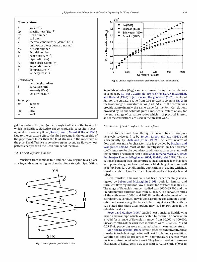
Transition from laminar to turbulent flow regime takes placet a Reynolds number higher than that for a straight pipe. Critical
Fig. 1. Basic geometry of a helical pipe.
Fig. 2. Critical Reynolds number predicted by various correlations.
Reynolds number (Recr) can be estimated using the correlationsdeveloped by Ito (1959), Schmidt (1967), Srinivasan, Nandapurkar,and Holland (1970) or Janssen and Hoogendoorn (1978). A plot ofRecr for the curvature ratio from 0.01 to 0.25 is given in Fig. 2. Inthe lower range of curvature ratios (ı < 0.05), all of the correlationsprovide approximately the same value for the Recr. Correlationsprovided by Ito and Schmidt gives almost equal values of Recr forthe entire range of curvature ratios which is of practical interestand these correlations are used in the present work.
1.3. Review of heat transfer in turbulent flows
Heat transfer and flow through a curved tube is compre-hensively reviewed first by Berger, Talbot, and Yao (1983) andsubsequently by Shah and Joshi (1987). The latest review offlow and heat transfer characteristics is provided by Naphon andWongwises (2006). Most of the investigations on heat transfercoefficients are for the boundary conditions such as constant walltemperature or constant heat flux (Nandakumar & Masliyah, 1982;Prabhanjan, Rennie, & Raghavan, 2004; Shah & Joshi, 1987). The sit-uation of constant wall temperature is idealised in heat exchangerswith phase change such as condensers. Modelling of constant wallheat flux boundary condition find applications in dealing with heattransfer studies of nuclear fuel elements and electrically heatedtubes.
Heat transfer in helical coils has been experimentally inves-tigated by Seban and McLaughlin (1963) both for laminar andturbulent flow regimes for flow of water for constant wall flux BC.The range of Reynolds number studied was 6000–65,500 and thePrandtl number variation was from 2.9 to 5.7. The curvature ratiosof the coils were 0.0096 and 0.0588. In the development of thecorrelation, data reduction was done assuming constant fluid prop-erties and considering the tubes to be straight ones. The authorshad stated that these assumptions may lead to 10% error in thecalculated values.
Rogers and Mayhew (1964) studied heat transfer to fluid flowinginside a helical pipe which was heated by steam. The correlationis valid for a range of Reynolds number from 10,000 to 100,000.Curvature ratios of the coils used in studies were 0.0926, 0.075 and0.05. Fluid properties were estimated at bulk mean temperature.
Mori and Nakayama (1967a) investigated forced convective heat
transfer in turbulent regime for wall heat flux boundary condition.Variation of physical properties with temperature changes werenot taken into account in their work. They have considered two con-figurations of helical coils, viz., coils with curvature ratio of 0.0535
4 Chem
attrsNu
Ytls(LcrLtpwsa
ebfat
mpEit(ocioet
hrafcumf
(tceAhw
taRngbl
sity of 9.963e8 cells m does not decrease the energy and masserrors in any appreciable way and mesh with this density is chosenfor analysis.
Pressure velocity coupling was done using the SIMPLEC scheme.Momentum equations were discretised using QUICK scheme. The
32 J.S. Jayakumar et al. / Computers and
nd 0.025. Subsequently Mori and Nakayama (1967b) studied heatransfer under constant wall temperature boundary condition forhe same helical coils. They observed that the Nusselt number isemarkably affected by a secondary flow due to curvature. Theytated that the same formula, which was used for estimation ofusselt number for wall heat flux boundary condition, could besed for the wall temperature boundary condition as well.
Heat transfer and pressure drop in helical pipes was studied byildiz, Bicer, and Pehlivan (1997). They have studied both emptyube and with heat transfer enhancement. Fully developed turbu-ent forced convective heat transfer in a helical coil, which has aubstantial coil pitch was numerically studied by Yang and Ebadian1996). Standard k − ε model with the constants recommended byaunder and Spalding (1972) were used in this study. They did notonsider any physical property variation and no generalised cor-elation was developed for estimation of heat transfer coefficients.in and Ebadian (1997) applied the same turbulence model to studyhe developing turbulent heat transfer in a helical coil of definiteitch for a constant wall temperature case. The FLUENT/UNS codeas used as the numerical solver. Subsequently the effect of inten-
ity of inlet turbulence on heat transfer rates was studied by Linnd Ebadian (1999) using the same numerical solver, FLUENT/UNS.
Guo, Chen, Feng, and Bai (1998) has developed correlations forstimation of Nusselt number for steady state and pulsating tur-ulent flow through helical coils in the range of Reynolds numberrom 6000 to 180,000. However this correlation does not includeny coil parameters (such as curvature ratio) and is applicable onlyo their setup.
Li, Lin, and Ebadian (1998) numerically investigated turbulentixed convective heat transfer in the entrance region of curved
ipes for constant wall temperature boundary condition using FLU-NT/UNS code. No correlation for prediction of heat transfer ratess provided by the authors. An experimental study of turbulent heatransfer in a horizontally coiled helical tube was done by Bai et al.1999), where the working fluid was heated by resistance heatingf the tube wall by passage of alternating current. However, theorrelation is not expressed in terms of Dean number as they havenvestigated heat transfer in only one coil. From their results, it isbserved that the average Nusselt number for a horizontally ori-nted helical tube is less than that for a vertically oriented one forhe same conditions.
Chagny, Castelain, and Peerhossaini (2000) studied the chaoticeat transfer in heat exchanger designs and compared them withegular regimes for a range of Reynolds numbers from 30 to 30,000nd for a number of Prandtl numbers. Pressure drop and heat trans-er in tube-in-tube helical heat exchanger under turbulent flowonditions was studied by Kumar, Saini, Sharma and Nigam (2006)sing the CFD package FLUENT 6. They have used the Wilson plotethod (Wilson, 1915) for data reduction. However, no correlation
or estimation of Nu was given in the paper.Recently Jayakumar, Mahajani, Mandal, Vijayan, and Bhoi
2008) have developed a correlation for estimation of inside heatransfer coefficient for flow of single-phase water through helicallyoiled heat exchangers. The correlation, which is validated againstxperiments, is applicable to a specific configuration of helical coils.lso the results presented in the paper describe only the overalleat transfer coefficient. The local variation of the Nusselt numberas not reported.
It can be seen that influence of various coil parameters are nothoroughly studied numerically so as to enable the generation ofcorrelation for prediction of Nusselt number. Also the ranges of
eynolds number and curvature ratio in the previous studies didot cover the whole of the possible operating ranges. The investi-ations reported for estimation of Nusselt number were found toe carried out with constant fluid properties. Also the publishediterature lacks much detail in the finer aspects of local heat trans-
ical Engineering 34 (2010) 430–446
fer rates and the fluid flow characteristics inside the helical coils.In the present work, variations of Nusselt number along the cir-cumference of the pipe and along the length of the coil have beenpresented. Much insight has been brought out regarding the natureof fluid flow inside a helical pipe.
In the next section, characteristics of fluid flow and heat transferin a helical pipe are presented. Helical coils of 12 different configu-rations have been analysed and the dependency of coil parameterson local and average Nusselt number is brought out. Using resultsof these computations, where temperature dependant fluid prop-erties are used, correlations for estimation of inside heat transfercoefficient for flow of single-phase water through helical coils aredeveloped. Further, variation of Nusselt number around the periph-ery at a given pipe cross-section is analysed and a correlation forprediction of local Nusselt number as a function of average Nusseltnumber and angular position is presented.
2. Nature of turbulent flow and heat transfer in helical coils
Analysis with heat transfer to water flowing through a helicalcoil is carried out using CFD package FLUENT version 6.3. As a rep-resentative case, coil of PCD = 200 mm and coil pitch of 30 mm ispresented for discussion. Diameter of the pipe used in the coil is20 mm. The geometry and the mesh were created using GAMBIT 2.3of the FLUENT package starting from its primitives. Boundary layermesh was generated for the pipe fluid volume. The Grid used forthis analysis is given in Fig. 3. This is the optimised grid after the gridindependency studies which has been detailed out in Jayakumar etal. (2008). The mesh density was changed from 3.5563e8 cells m−3
to 12.365e8 cells m−3. It is found that refinement after a mesh den-−3
Fig. 3. (a). Grid of the helical pipe used for analysis. (b) Grid at any cross-section ofthe helical pipe.
Chemical Engineering 34 (2010) 430–446 433
r1iga
ewdD(sw
efiafl
opwlhFftmclSelu
cdbr
T
wTtds
N
wd
m
N
it
N
Table 1Boundary conditions.
Field variable Inlet Walls Outlet
u 0.8 m s−1 0.0 ∂u/∂n = 0v 0.0 0.0 ∂v/∂n = 0
J.S. Jayakumar et al. / Computers and
ealizable k − ε turbulence model (Shih, Liou, Shabbir, Yang, & Zhu,995) is used in these computations. This scheme is ideal for flows
nvolving rotation, boundary layers under strong adverse pressureradients, separation, and recirculation (Kim et al., 1997; Shih etl., 1995; Fluent, 2007).
Power law scheme of discretisation is used for turbulent kineticnergy and dissipation rate equations. Convergence criterion usedas 1.0e−5 for continuity, velocities, k, and ε. Temperature depen-ent properties as polynomial functions were used for water.etails of the modelling equations are available in Jayakumar et al.
2008). For the energy equation third order QUICK discretisationcheme was employed. Convergence criterion for energy balanceas 1.0e−07.
The results of simulation are exported as a CGNS (CFD Gen-ral Notation System, http://www.cgns.org) file from Fluent. Theelds exported are pressure, temperature, velocity magnitude,xial, radial and tangential velocity, wall temperature, wall heatux, density, specific heat and thermal conductivity.
For post-processing a visualisation package AnuVi devel-ped by Computer Division, BARC is used. AnuVi is a cross-latform CFD post-processor and Scientific Visualisation Frame-ork and is built on top of the open source software
ike Python (http://www.python.org), Visualization ToolKit (VTK,ttp://www.vtk.org), WxWidgets (http://www.wxwidgets.org) andFmpeg (http://www.ffmpeg.org). It can handle many standard fileormats like CGNS, PLOT3D, VTK, STL, OBJ, BYU and PLY and has fea-ures to provide animation, extraction and derivation of data over
any data components with advanced graphics (including shading,ontouring, lighting and transparency). The package has featuresike Session Handling, Seamless Data integration, Python Languagecripting, etc. Rendering is handled by OpenGL and can be accel-rated with advanced graphics hardware. The feature of Pythonanguage scripting gives unlimited control to user which can besed for automation of data extraction and visualisation.
For extraction of data and visualisation, the CGNS files are pro-essed to create planes at desired spacing in the computationalomain. Since the fluid properties are temperature dependent, theulk fluid temperature at a cross-section is evaluated using theelation,
b =∫
u�CpTdA∫u�CpdA
, (3)
here dA is an elemental area of the pipe cross-section (see Fig. 3b).he wall temperatures at four locations (inner, outer, top and bot-om of the pipe) in a cross-section are also extracted. Using theseata, values of local Nusselt number at four locations at that cross-ection are calculated using the formula,
uloc = 2r
k
(q′′
Tw − Tb
). (4)
here heat flux is calculated by, q′′ = k(∂T/∂n)w; n is the normalirection.
As used by Lin and Ebadian (1997), average Nu at a cross-sectionay be estimated by,
uav = 12�
∫ 2�
0
(Nu�)d�. (5)
But this does not ensure that the Nusselt number so estimated
s representative of the total heat flux in that cross-section. Hence,he mean Nusselt number is evaluated by;uav = 2r
km
(q′′
mTw,m − Tb
). (6)
w 0.0 0.0 ∂w/∂n = 0T 330 K 300 K ∂T/∂n = 0P ∂P/∂n = 0 ∂P/∂n = 0 0.0
Here km, Tw,m and q′′m are evaluated by the formula,
ϕm =∫ 2�
0(ϕA)d�∫ 2�
0(A)d�
. (7)
where �, k, Tw or q′′ as the case may be and A is an elemental areaof a ring along the wall to which the parameter is associated to.
The above sets of operations are repeated at successive planes tocover the entire length of the pipe. All of the above processing havebeen done using Python scripts which runs on top of the AnuVipackage. Various programs required to generate the cut planes,etc. was written in c++ programming language. MATLAB® has beenextensively used for processing of the extracted data and regressionanalysis.
The remaining parts of this section describe the results of analy-sis carried out with constant wall temperature boundary conditionand constant wall heat flux boundary condition.
2.1. Constant wall temperature boundary condition
In this analysis hot water at 330 K temperature and 0.8 ms−1
velocity is entering the helical pipe at the top, where an inlet veloc-ity boundary condition is specified. The flow velocity is such thatthe flow regime is turbulent. The fluid is made to cool down as itflows along the tube by specifying a wall temperature of 300 K. Thefluid properties are estimated as per Eqs. (8a)–(8d). More details areavailable in Jayakumar et al. (2008). At the pipe wall, for the energyequation, a Dirichlet boundary condition and for momentum andpressure equations homogenous Neumann boundary condition arespecified. At the inlet a turbulent intensity of 4% and hydraulicdiameter of the largest size eddy, which is taken as 0.3 times pipeinner diameter, are specified. At the outlet, a pressure outlet bound-ary is enforced. Summary of the boundary conditions is given inTable 1.
�(T) = 2.1897e − 11T4 − 3.055e − 8T3 + 1.6028e − 5T2
− 0.0037524T + 0.33158 (8a)
�(T) = −1.5629e − 5T3 + 0.011778T2 − 3.0726T + 1227.8 (8b)
k(T)=1.5362e − 8T3−2.261e − 05T2 + 0.010879T − 1.0294 (8c)
Cp(T) = 1.1105e − 5T3 − 0.0031078T2 − 1.478T + 4631.9 (8d)
Fig. 4(a) shows an overview of velocity contours at varioussections along the length of the coil, while the details at a few cross-sections are available in Fig. 4(b). The planes are identified by theangle (�) which that plane makes with the plane passing throughthe pipe inlet. In Fig. 4(a), the first plane shown on the top is at10◦ from the inlet (i.e., � = 10◦) and the subsequent planes are 10◦
apart.Up to an angle of � = 35◦, the velocity profile at a cross-section is
found to be symmetric. Subsequently, this uniform velocity patternchanges to a pattern with a high velocity region located at the outerside of the coil. This behaviour is seen predominantly by � = 45◦ andcontinues to develop. It can be seen that by � = 135◦, the high veloc-ity region is present only in outer half cross-section. Area of high
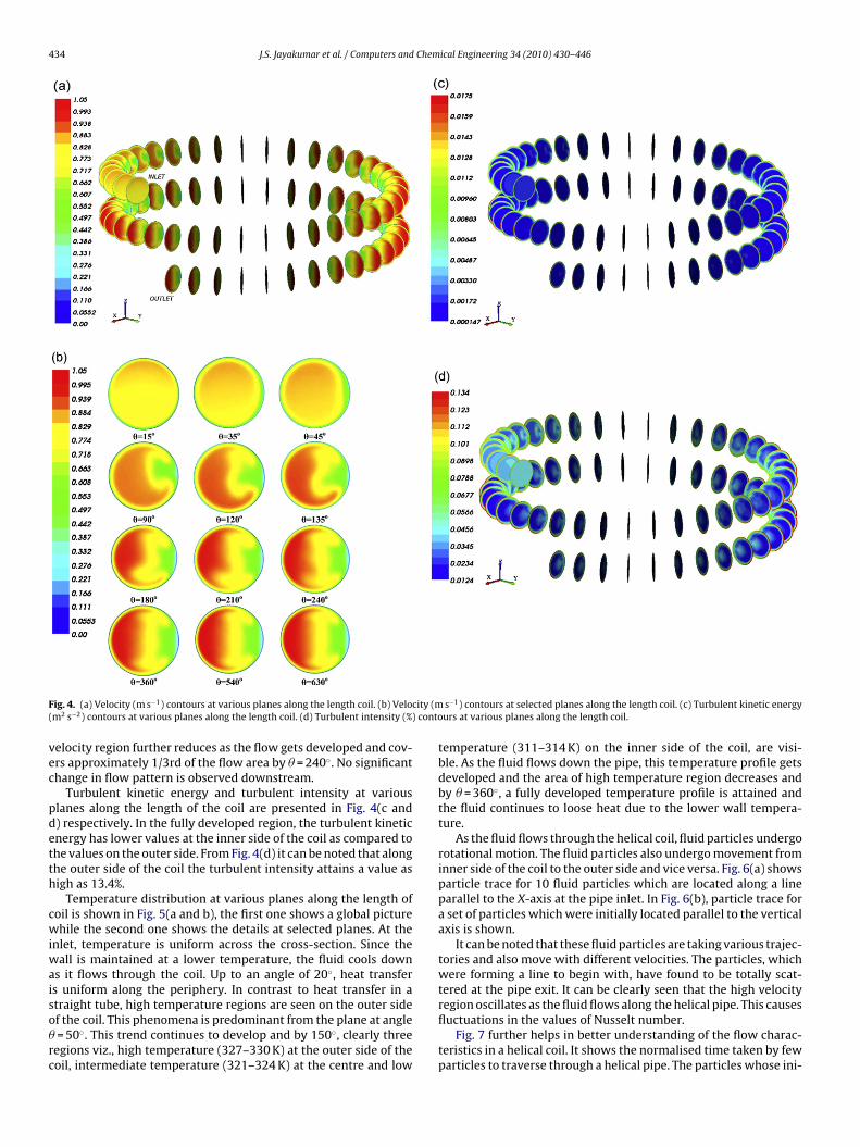
434 J.S. Jayakumar et al. / Computers and Chemical Engineering 34 (2010) 430–446
F city (m( conto
vec
pdetth
cwiwaiso�rc
ig. 4. (a) Velocity (m s−1) contours at various planes along the length coil. (b) Velom2 s−2) contours at various planes along the length coil. (d) Turbulent intensity (%)
elocity region further reduces as the flow gets developed and cov-rs approximately 1/3rd of the flow area by � = 240◦. No significanthange in flow pattern is observed downstream.
Turbulent kinetic energy and turbulent intensity at variouslanes along the length of the coil are presented in Fig. 4(c and) respectively. In the fully developed region, the turbulent kineticnergy has lower values at the inner side of the coil as compared tohe values on the outer side. From Fig. 4(d) it can be noted that alonghe outer side of the coil the turbulent intensity attains a value asigh as 13.4%.
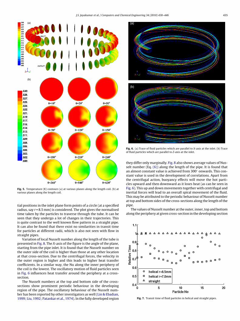
Temperature distribution at various planes along the length ofoil is shown in Fig. 5(a and b), the first one shows a global picturehile the second one shows the details at selected planes. At the
nlet, temperature is uniform across the cross-section. Since theall is maintained at a lower temperature, the fluid cools down
s it flows through the coil. Up to an angle of 20◦, heat transfers uniform along the periphery. In contrast to heat transfer in a
traight tube, high temperature regions are seen on the outer sidef the coil. This phenomena is predominant from the plane at angle= 50◦. This trend continues to develop and by 150◦, clearly threeegions viz., high temperature (327–330 K) at the outer side of theoil, intermediate temperature (321–324 K) at the centre and low
s−1) contours at selected planes along the length coil. (c) Turbulent kinetic energyurs at various planes along the length coil.
temperature (311–314 K) on the inner side of the coil, are visi-ble. As the fluid flows down the pipe, this temperature profile getsdeveloped and the area of high temperature region decreases andby � = 360◦, a fully developed temperature profile is attained andthe fluid continues to loose heat due to the lower wall tempera-ture.
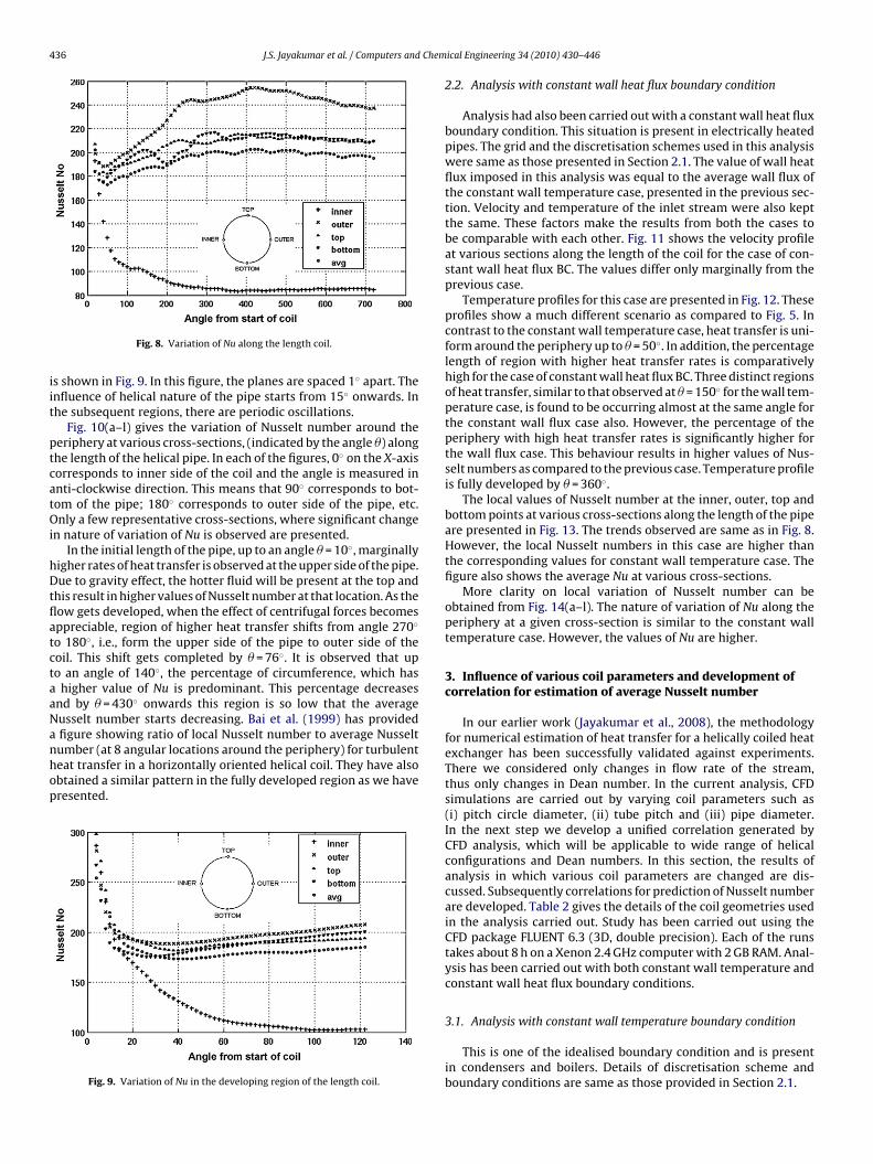
As the fluid flows through the helical coil, fluid particles undergorotational motion. The fluid particles also undergo movement frominner side of the coil to the outer side and vice versa. Fig. 6(a) showsparticle trace for 10 fluid particles which are located along a lineparallel to the X-axis at the pipe inlet. In Fig. 6(b), particle trace fora set of particles which were initially located parallel to the verticalaxis is shown.
It can be noted that these fluid particles are taking various trajec-tories and also move with different velocities. The particles, whichwere forming a line to begin with, have found to be totally scat-tered at the pipe exit. It can be clearly seen that the high velocity
region oscillates as the fluid flows along the helical pipe. This causesfluctuations in the values of Nusselt number.Fig. 7 further helps in better understanding of the flow charac-teristics in a helical coil. It shows the normalised time taken by fewparticles to traverse through a helical pipe. The particles whose ini-
J.S. Jayakumar et al. / Computers and Chemical Engineering 34 (2010) 430–446 435
Fv
trtsiIfs
pstatctis
srb1
at top and bottom sides of the cross-sections along the length of thepipe.
The values of Nusselt number at the outer, inner, top and bottomalong the periphery at given cross-section in the developing section
ig. 5. Temperature (K) contours (a) at various planes along the length coil. (b) atarious planes along the length coil.
ial positions in the inlet plane form points of a circle (at a specifiedadius, say r = 8.5 mm) is considered. The plot gives the normalisedime taken by the particles to traverse through the tube. It can beeen that they undergo a lot of changes in their trajectories. Thiss quite contrast to the well known flow pattern in a straight pipe.t can also be found that there exist no similarities in transit timeor particles at different radii, which is also not seen with flow intraight pipes.
Variation of local Nusselt number along the length of the tube isresented in Fig. 8. The X-axis of the figure is the angle of the plane,tarting from the pipe inlet. It is found that the Nusselt number onhe outer side of the coil is higher than those at any other locationt that cross-section. Due to the centrifugal forces, the velocity inhe outer region is higher and this leads to higher heat transferoefficients. In a similar way, the Nu along the inner periphery ofhe coil is the lowest. The oscillatory motion of fluid particles seenn Fig. 6 influences heat transfer around the periphery at a cross-ection.
The Nusselt numbers at the top and bottom side of the cross-
ections show prominent periodic behaviour in the developingegion of the pipe. The oscillatory behaviour of the Nusselt num-er has been reported by other investigators as well (Lin & Ebadian,999; Liu, 1992; Patankar et al., 1974). In the fully developed regionFig. 6. (a) Trace of fluid particles which are parallel to X-axis at the inlet. (b) Traceof fluid particles which are parallel to Z-axis at the inlet.
they differ only marginally. Fig. 8 also shows average values of Nus-selt number (Eq. (6)) along the length of the pipe. It is found thatan almost constant value is achieved from 300◦ onwards. This con-stant value is used in the development of correlations. Apart fromthe centrifugal action, buoyancy effects will move the hot parti-cles upward and then downward as it loses heat (as can be seen inFig. 6). This up and down movements together with centrifugal andinertial forces will lead to an overall spiral movement of the fluid.This may be attributed to the periodic behaviour of Nusselt number
Fig. 7. Transit time of fluid particles in helical and straight pipes.
436 J.S. Jayakumar et al. / Computers and Chem
iit
ptcatOi
hDtflatctaaNanhop
Fig. 8. Variation of Nu along the length coil.
s shown in Fig. 9. In this figure, the planes are spaced 1◦ apart. Thenfluence of helical nature of the pipe starts from 15◦ onwards. Inhe subsequent regions, there are periodic oscillations.
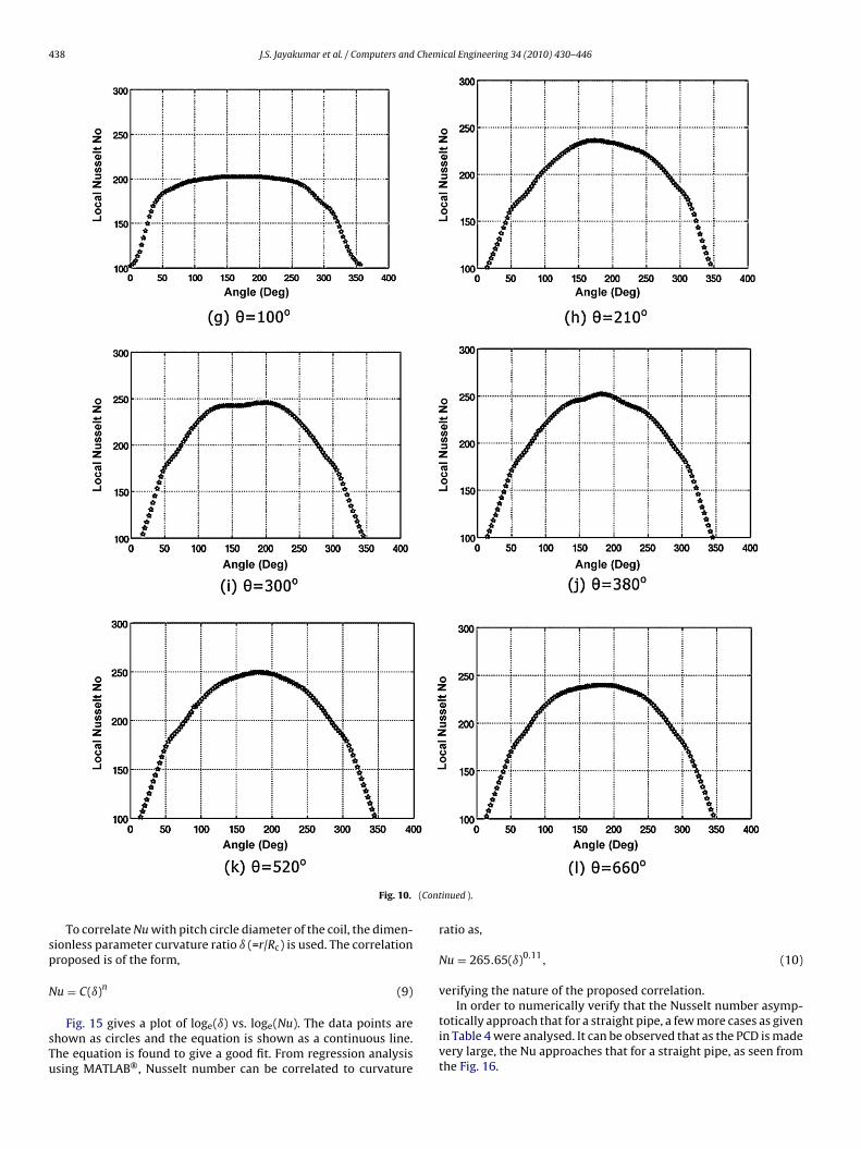
Fig. 10(a–l) gives the variation of Nusselt number around theeriphery at various cross-sections, (indicated by the angle �) alonghe length of the helical pipe. In each of the figures, 0◦ on the X-axisorresponds to inner side of the coil and the angle is measured innti-clockwise direction. This means that 90◦ corresponds to bot-om of the pipe; 180◦ corresponds to outer side of the pipe, etc.nly a few representative cross-sections, where significant change
n nature of variation of Nu is observed are presented.In the initial length of the pipe, up to an angle � = 10◦, marginally
igher rates of heat transfer is observed at the upper side of the pipe.ue to gravity effect, the hotter fluid will be present at the top and
his result in higher values of Nusselt number at that location. As theow gets developed, when the effect of centrifugal forces becomesppreciable, region of higher heat transfer shifts from angle 270◦
o 180◦, i.e., form the upper side of the pipe to outer side of theoil. This shift gets completed by � = 76◦. It is observed that upo an angle of 140◦, the percentage of circumference, which has
higher value of Nu is predominant. This percentage decreasesnd by � = 430◦ onwards this region is so low that the averageusselt number starts decreasing. Bai et al. (1999) has providedfigure showing ratio of local Nusselt number to average Nusselt
umber (at 8 angular locations around the periphery) for turbulenteat transfer in a horizontally oriented helical coil. They have alsobtained a similar pattern in the fully developed region as we haveresented.Fig. 9. Variation of Nu in the developing region of the length coil.
ical Engineering 34 (2010) 430–446
2.2. Analysis with constant wall heat flux boundary condition
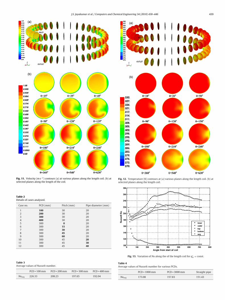
Analysis had also been carried out with a constant wall heat fluxboundary condition. This situation is present in electrically heatedpipes. The grid and the discretisation schemes used in this analysiswere same as those presented in Section 2.1. The value of wall heatflux imposed in this analysis was equal to the average wall flux ofthe constant wall temperature case, presented in the previous sec-tion. Velocity and temperature of the inlet stream were also keptthe same. These factors make the results from both the cases tobe comparable with each other. Fig. 11 shows the velocity profileat various sections along the length of the coil for the case of con-stant wall heat flux BC. The values differ only marginally from theprevious case.
Temperature profiles for this case are presented in Fig. 12. Theseprofiles show a much different scenario as compared to Fig. 5. Incontrast to the constant wall temperature case, heat transfer is uni-form around the periphery up to � = 50◦. In addition, the percentagelength of region with higher heat transfer rates is comparativelyhigh for the case of constant wall heat flux BC. Three distinct regionsof heat transfer, similar to that observed at � = 150◦ for the wall tem-perature case, is found to be occurring almost at the same angle forthe constant wall flux case also. However, the percentage of theperiphery with high heat transfer rates is significantly higher forthe wall flux case. This behaviour results in higher values of Nus-selt numbers as compared to the previous case. Temperature profileis fully developed by � = 360◦.
The local values of Nusselt number at the inner, outer, top andbottom points at various cross-sections along the length of the pipeare presented in Fig. 13. The trends observed are same as in Fig. 8.However, the local Nusselt numbers in this case are higher thanthe corresponding values for constant wall temperature case. Thefigure also shows the average Nu at various cross-sections.
More clarity on local variation of Nusselt number can beobtained from Fig. 14(a–l). The nature of variation of Nu along theperiphery at a given cross-section is similar to the constant walltemperature case. However, the values of Nu are higher.
3. Influence of various coil parameters and development ofcorrelation for estimation of average Nusselt number
In our earlier work (Jayakumar et al., 2008), the methodologyfor numerical estimation of heat transfer for a helically coiled heatexchanger has been successfully validated against experiments.There we considered only changes in flow rate of the stream,thus only changes in Dean number. In the current analysis, CFDsimulations are carried out by varying coil parameters such as(i) pitch circle diameter, (ii) tube pitch and (iii) pipe diameter.In the next step we develop a unified correlation generated byCFD analysis, which will be applicable to wide range of helicalconfigurations and Dean numbers. In this section, the results ofanalysis in which various coil parameters are changed are dis-cussed. Subsequently correlations for prediction of Nusselt numberare developed. Table 2 gives the details of the coil geometries usedin the analysis carried out. Study has been carried out using theCFD package FLUENT 6.3 (3D, double precision). Each of the runstakes about 8 h on a Xenon 2.4 GHz computer with 2 GB RAM. Anal-ysis has been carried out with both constant wall temperature andconstant wall heat flux boundary conditions.
3.1. Analysis with constant wall temperature boundary condition
This is one of the idealised boundary condition and is presentin condensers and boilers. Details of discretisation scheme andboundary conditions are same as those provided in Section 2.1.
Chem
3
wwo
icflca
J.S. Jayakumar et al. / Computers and
.1.1. Influence of pitch circle diameter (PCD)The coils with PCDs 100 mm, 200 mm, 300 mm and 400 mm
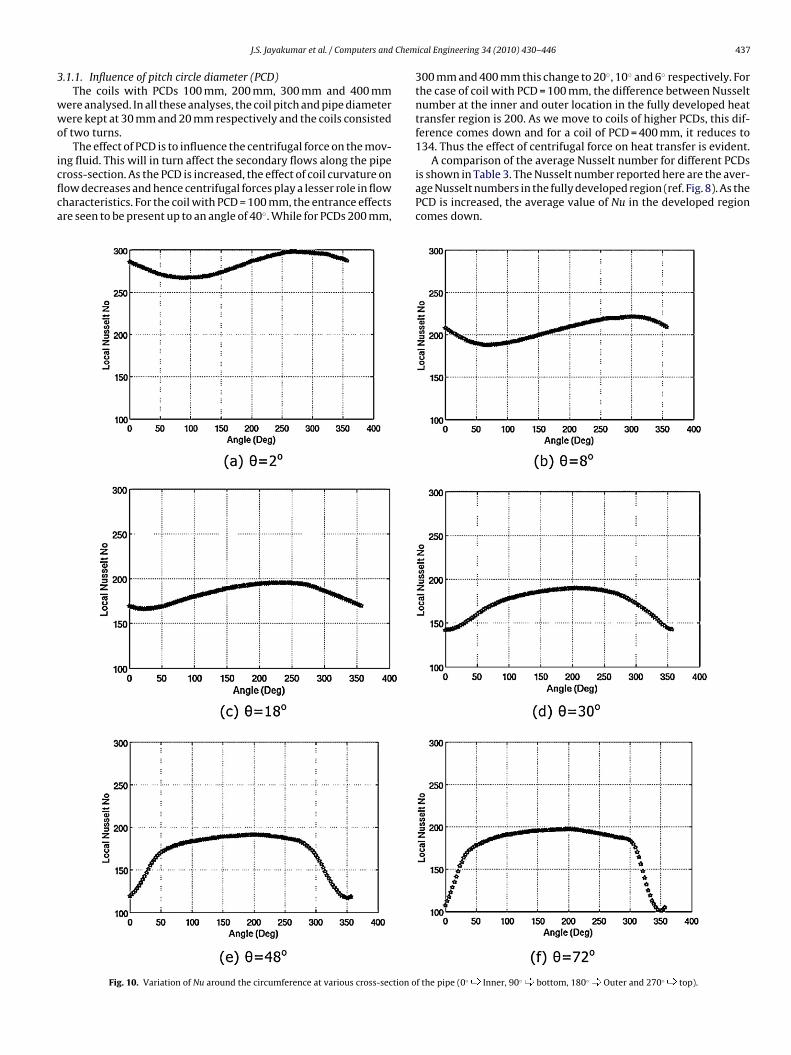
ere analysed. In all these analyses, the coil pitch and pipe diameterere kept at 30 mm and 20 mm respectively and the coils consisted
f two turns.The effect of PCD is to influence the centrifugal force on the mov-
ng fluid. This will in turn affect the secondary flows along the pipeross-section. As the PCD is increased, the effect of coil curvature onow decreases and hence centrifugal forces play a lesser role in flowharacteristics. For the coil with PCD = 100 mm, the entrance effectsre seen to be present up to an angle of 40◦. While for PCDs 200 mm,
Fig. 10. Variation of Nu around the circumference at various cross-section o
ical Engineering 34 (2010) 430–446 437
300 mm and 400 mm this change to 20◦, 10◦ and 6◦ respectively. Forthe case of coil with PCD = 100 mm, the difference between Nusseltnumber at the inner and outer location in the fully developed heattransfer region is 200. As we move to coils of higher PCDs, this dif-ference comes down and for a coil of PCD = 400 mm, it reduces to134. Thus the effect of centrifugal force on heat transfer is evident.
A comparison of the average Nusselt number for different PCDsis shown in Table 3. The Nusselt number reported here are the aver-age Nusselt numbers in the fully developed region (ref. Fig. 8). As thePCD is increased, the average value of Nu in the developed regioncomes down.
f the pipe (0◦ Inner, 90◦ bottom, 180◦ Outer and 270◦ top).
438 J.S. Jayakumar et al. / Computers and Chemical Engineering 34 (2010) 430–446
(Cont
sp
N
sTu
Fig. 10.
To correlate Nu with pitch circle diameter of the coil, the dimen-ionless parameter curvature ratio ı (=r/Rc) is used. The correlationroposed is of the form,
u = C(ı)n (9)
Fig. 15 gives a plot of loge(ı) vs. loge(Nu). The data points arehown as circles and the equation is shown as a continuous line.he equation is found to give a good fit. From regression analysissing MATLAB®, Nusselt number can be correlated to curvature
inued ).
ratio as,
Nu = 265.65(ı)0.11, (10)
verifying the nature of the proposed correlation.
In order to numerically verify that the Nusselt number asymp-totically approach that for a straight pipe, a few more cases as givenin Table 4 were analysed. It can be observed that as the PCD is madevery large, the Nu approaches that for a straight pipe, as seen fromthe Fig. 16.
J.S. Jayakumar et al. / Computers and Chemical Engineering 34 (2010) 430–446 439
Fig. 11. Velocity (m s−1) contours (a) at various planes along the length coil. (b) atselected planes along the length of the coil.
Table 2Details of cases analysed.
Case no. PCD (mm) Pitch (mm) Pipe diameter (mm)
1 100 30 202 200 30 203 300 30 204 400 30 205 300 0 206 300 15 207 300 30 208 300 45 209 300 60 20
10 300 45 2011 300 45 3012 300 45 40
Table 3Average values of Nusselt number.
PCD = 100 mm PCD = 200 mm PCD = 300 mm PCD = 400 mm
Nuavg 226.33 208.23 197.65 192.04
Fig. 12. Temperature (K) contours at (a) various planes along the length coil. (b) atselected planes along the length coil.
Fig. 13. Variation of Nu along the of the length coil for q′′w = const.
Table 4Average values of Nusselt number for various PCDs.
PCD = 1000 mm PCD = 3000 mm Straight pipe
Nuavg 173.08 157.83 151.43
4 Chem
3
2Aoa
aFo
ence between the local Nusselt numbers at the top and bottom at
40 J.S. Jayakumar et al. / Computers and
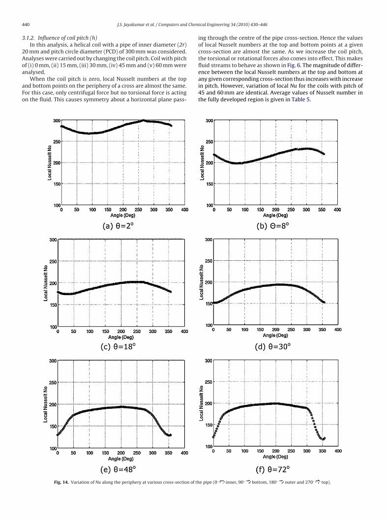
.1.2. Influence of coil pitch (h)In this analysis, a helical coil with a pipe of inner diameter (2r)
0 mm and pitch circle diameter (PCD) of 300 mm was considered.nalyses were carried out by changing the coil pitch. Coil with pitchf (i) 0 mm, (ii) 15 mm, (iii) 30 mm, (iv) 45 mm and (v) 60 mm werenalysed.
When the coil pitch is zero, local Nusselt numbers at the topnd bottom points on the periphery of a cross are almost the same.or this case, only centrifugal force but no torsional force is actingn the fluid. This causes symmetry about a horizontal plane pass-
Fig. 14. Variation of Nu along the periphery at various cross-section of th
ical Engineering 34 (2010) 430–446
ing through the centre of the pipe cross-section. Hence the valuesof local Nusselt numbers at the top and bottom points at a givencross-section are almost the same. As we increase the coil pitch,the torsional or rotational forces also comes into effect. This makesfluid streams to behave as shown in Fig. 6. The magnitude of differ-
e pipe (0◦ inner, 90◦ bottom, 180◦ outer and 270◦ top).
any given corresponding cross-section thus increases with increasein pitch. However, variation of local Nu for the coils with pitch of45 and 60 mm are identical. Average values of Nusselt number inthe fully developed region is given in Table 5.
J.S. Jayakumar et al. / Computers and Chemical Engineering 34 (2010) 430–446 441
(Cont
pT1
TA
Fig. 14.
It is found that the Nuavg increases marginally with increase initch and almost insensitive to its further changes at higher pitches.he percentage increase, when the pitch is changed from 0 mm to5 mm is about 1% and this value changes to 0.2% when the pitch
able 5verage values of Nusselt number for various coil pitches.
H = 0 mm H = 15 mm H = 30 mm H = 45 mm H = 60 mm
Nuavg 189.24 191.08 191.75 192.27 192.55
inued ).
is changed from 45 mm to 60 mm. For any engineering applica-tion, the tube pitch has to be higher than pipe diameter and inthat range the changes in Nuavg due to changes in pitch are neg-ligible. Hence the effect of coil pitch on overall heat transfer fordesign purposes need not be considered for most of the practi-cal applications with helical coils. However, it has implications in
heat transfer in the developing regions. The maximum differencein Nusselt number between the top and bottom locations is givenin Table 6. This clearly shows the extent of oscillatory behaviour.Another observation is the shift of the symmetry in temperature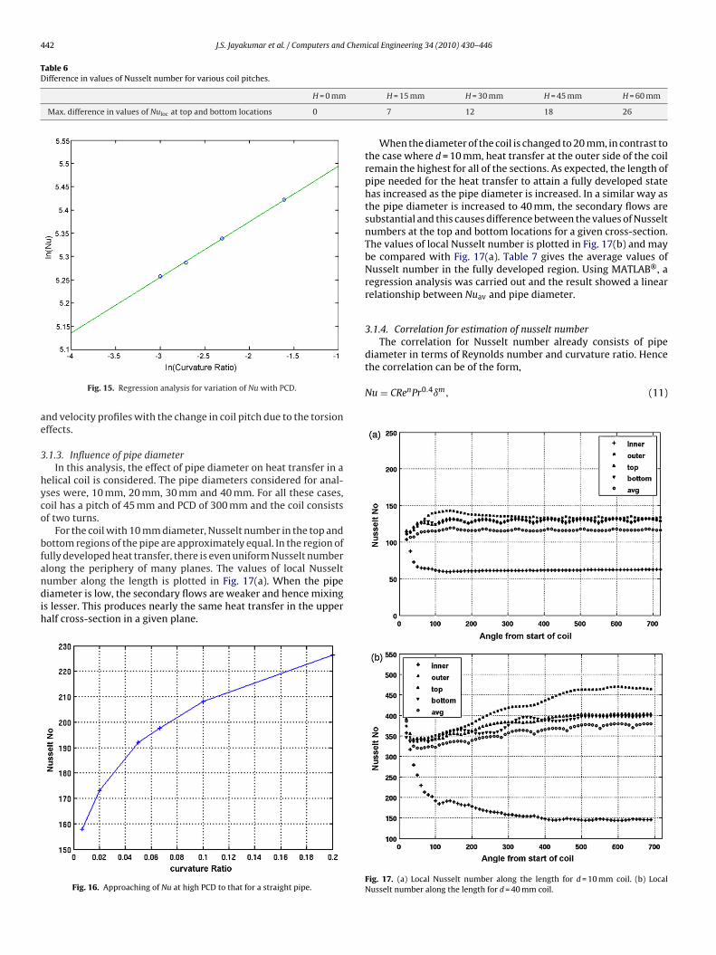
442 J.S. Jayakumar et al. / Computers and Chemical Engineering 34 (2010) 430–446
Table 6Difference in values of Nusselt number for various coil pitches.
H = 0 mm
Max. difference in values of Nuloc at top and bottom locations 0
ae
3
hyco
bfandih
diameter in terms of Reynolds number and curvature ratio. Hencethe correlation can be of the form,
Nu = CRenPr0.4ım, (11)
Fig. 15. Regression analysis for variation of Nu with PCD.nd velocity profiles with the change in coil pitch due to the torsionffects.
.1.3. Influence of pipe diameterIn this analysis, the effect of pipe diameter on heat transfer in a
elical coil is considered. The pipe diameters considered for anal-ses were, 10 mm, 20 mm, 30 mm and 40 mm. For all these cases,oil has a pitch of 45 mm and PCD of 300 mm and the coil consistsf two turns.
For the coil with 10 mm diameter, Nusselt number in the top andottom regions of the pipe are approximately equal. In the region ofully developed heat transfer, there is even uniform Nusselt number
long the periphery of many planes. The values of local Nusseltumber along the length is plotted in Fig. 17(a). When the pipeiameter is low, the secondary flows are weaker and hence mixings lesser. This produces nearly the same heat transfer in the upperalf cross-section in a given plane.
Fig. 16. Approaching of Nu at high PCD to that for a straight pipe.
H = 15 mm H = 30 mm H = 45 mm H = 60 mm
7 12 18 26
When the diameter of the coil is changed to 20 mm, in contrast tothe case where d = 10 mm, heat transfer at the outer side of the coilremain the highest for all of the sections. As expected, the length ofpipe needed for the heat transfer to attain a fully developed statehas increased as the pipe diameter is increased. In a similar way asthe pipe diameter is increased to 40 mm, the secondary flows aresubstantial and this causes difference between the values of Nusseltnumbers at the top and bottom locations for a given cross-section.The values of local Nusselt number is plotted in Fig. 17(b) and maybe compared with Fig. 17(a). Table 7 gives the average values ofNusselt number in the fully developed region. Using MATLAB®, aregression analysis was carried out and the result showed a linearrelationship between Nuav and pipe diameter.
3.1.4. Correlation for estimation of nusselt numberThe correlation for Nusselt number already consists of pipe
Fig. 17. (a) Local Nusselt number along the length for d = 10 mm coil. (b) LocalNusselt number along the length for d = 40 mm coil.
J.S. Jayakumar et al. / Computers and Chemical Engineering 34 (2010) 430–446 443
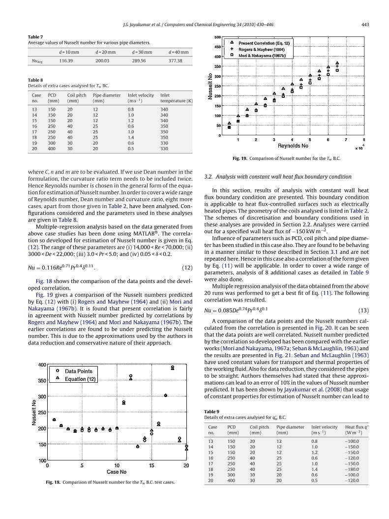
Table 7Average values of Nusselt number for various pipe diameters.
d = 10 mm d = 20 mm d = 30 mm d = 40 mm
Nuavg 116.39 200.03 289.56 377.38
Table 8Details of extra cases analysed for Tw BC.
Caseno.
PCD(mm)
Coil pitch(mm)
Pipe diameter(mm)
Inlet velocity(m s−1)
Inlettemperature (K)
13 150 20 12 0.8 34014 150 20 12 1.0 34015 150 20 12 1.2 34016 250 40 25 0.6 35017 250 40 25 1.0 350
wfHtocfia
at(3
N
o
bNiRend
18 250 40 25 1.4 35019 300 30 20 0.6 33020 400 30 20 0.5 330
here C, n and m are to be evaluated. If we use Dean number in theormulation, the curvature ratio term needs to be included twice.ence Reynolds number is chosen in the general form of the equa-
ion for estimation of Nusselt number. In order to cover a wide rangef Reynolds number, Dean number and curvature ratio, eight moreases, apart from those given in Table 2, have been analysed. Con-gurations considered and the parameters used in these analysesre given in Table 8.
Multiple-regression analysis based on the data generated frombove case studies has been done using MATLAB®. The correla-ion so developed for estimation of Nusselt number is given in Eq.12). The range of these parameters are (i) 14,000 < Re < 70,000; (ii)000 < De < 22,000; (iii) 3.0 < Pr < 5.0; and (iv) 0.05 < ı < 0.2.
u = 0.116Re0.71Pr0.4ı0.11. (12)
Fig. 18 shows the comparison of the data points and the devel-ped correlation.
Fig. 19 gives a comparison of the Nusselt numbers predictedy Eq. (12) with (i) Rogers and Mayhew (1964) and (ii) Mori andakayama (1967b). It is found that present correlation is fairly
n agreement with Nusselt number predicted by correlations byogers and Mayhew (1964) and Mori and Nakayama (1967b). The
arlier correlations are found to be under predicting the Nusseltumber. This is due to the approximations used by the authors inata reduction and conservative nature of their approach.Fig. 18. Comparison of Nusselt number for the Tw B.C. test cases.
Fig. 19. Comparison of Nusselt number for the Tw B.C.
3.2. Analysis with constant wall heat flux boundary condition
In this section, results of analysis with constant wall heatflux boundary condition are presented. This boundary conditionis applicable to heat flux-controlled surfaces such as electricallyheated pipes. The geometry of the coils analysed is listed in Table 2.The schemes of discretisation and boundary conditions used inthese analyses are provided in Section 2.2. Analyses were carriedout for a specified wall heat flux of −150 kW m−2.
Influence of parameters such as PCD, coil pitch and pipe diame-ter has been studied in this case also. They are found to be behavingin a manner similar to those described in Section 3.1 and are notrepeated here. Hence in this case also a correlation of the form givenby Eq. (11) will be applicable. In order to cover a wide range ofparameters, analysis of 8 additional cases as detailed in Table 9were also done.
Multiple regression analysis of the data obtained from the above20 runs was performed to get a best fit of Eq. (11). The followingcorrelation was resulted.
Nu = 0.085De0.74Pr0.4ı0.1 (13)
A comparison of the data points and the Nusselt numbers cal-culated from the correlation is presented in Fig. 20. It can be seenthat the data points are well correlated. Nusselt number predictedby the correlation so developed has been compared with the earlierworks (Mori and Nakayama, 1967a; Seban & McLaughlin, 1963) andthe results are presented in Fig. 21. Seban and McLaughlin (1963)have used constant values for transport and thermal properties of
the working fluid. Also for data reduction, they considered the pipesto be straight. Authors themselves had stated that these approxi-mations can lead to an error of 10% in the values of Nusselt numberpredicted. It has been shown by Jayakumar et al. (2008) that usageof constant properties for estimation of Nusselt number can lead toTable 9Details of extra cases analysed for q′′
w B.C.
Caseno.
PCD(mm)
Coil pitch(mm)
Pipe diameter(mm)
Inlet velocity(m s−1)
Heat flux q′′
(W m−2)
13 150 20 12 0.8 −100.014 150 20 12 1.0 −150.015 150 20 12 1.2 −150.016 250 40 25 0.6 −120.017 250 40 25 1.0 −150.018 250 40 25 1.4 −180.019 300 30 20 0.6 −100.020 400 30 20 0.5 −120.0
444 J.S. Jayakumar et al. / Computers and Chemical Engineering 34 (2010) 430–446
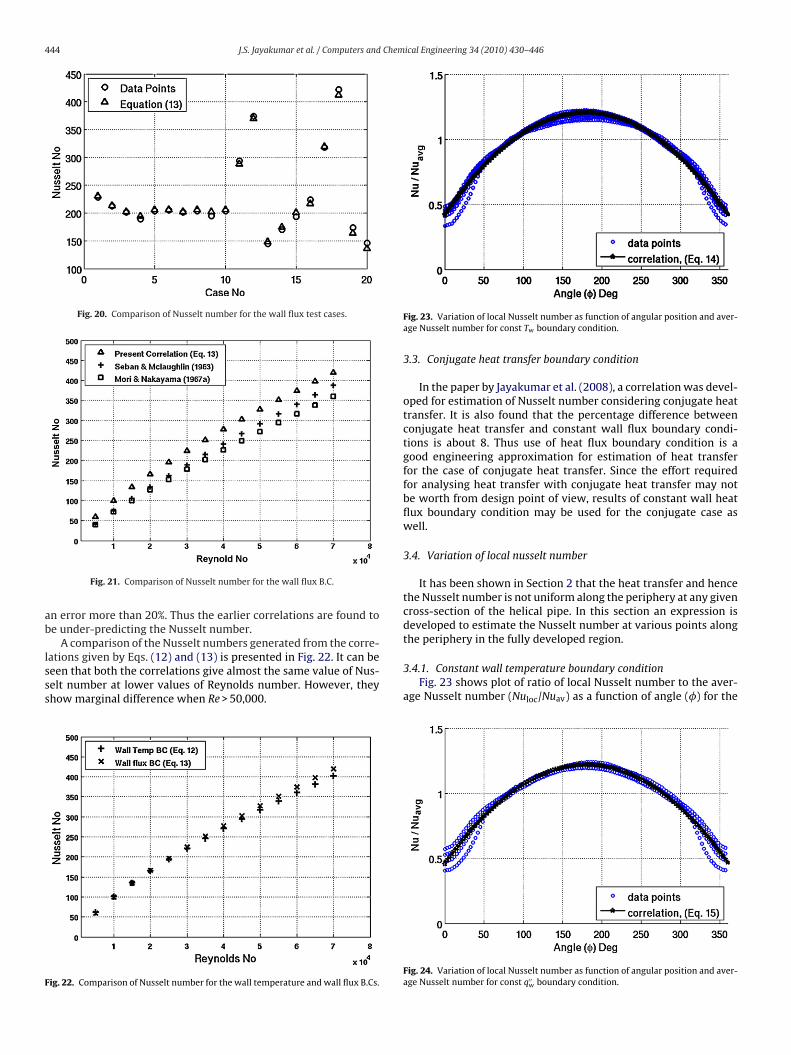
Fig. 20. Comparison of Nusselt number for the wall flux test cases.
ab
lsss
F
Fig. 21. Comparison of Nusselt number for the wall flux B.C.
n error more than 20%. Thus the earlier correlations are found toe under-predicting the Nusselt number.
A comparison of the Nusselt numbers generated from the corre-ations given by Eqs. (12) and (13) is presented in Fig. 22. It can be
een that both the correlations give almost the same value of Nus-elt number at lower values of Reynolds number. However, theyhow marginal difference when Re > 50,000.ig. 22. Comparison of Nusselt number for the wall temperature and wall flux B.Cs.
Fig. 23. Variation of local Nusselt number as function of angular position and aver-age Nusselt number for const Tw boundary condition.
3.3. Conjugate heat transfer boundary condition
In the paper by Jayakumar et al. (2008), a correlation was devel-oped for estimation of Nusselt number considering conjugate heattransfer. It is also found that the percentage difference betweenconjugate heat transfer and constant wall flux boundary condi-tions is about 8. Thus use of heat flux boundary condition is agood engineering approximation for estimation of heat transferfor the case of conjugate heat transfer. Since the effort requiredfor analysing heat transfer with conjugate heat transfer may notbe worth from design point of view, results of constant wall heatflux boundary condition may be used for the conjugate case aswell.
3.4. Variation of local nusselt number
It has been shown in Section 2 that the heat transfer and hencethe Nusselt number is not uniform along the periphery at any givencross-section of the helical pipe. In this section an expression isdeveloped to estimate the Nusselt number at various points alongthe periphery in the fully developed region.
3.4.1. Constant wall temperature boundary conditionFig. 23 shows plot of ratio of local Nusselt number to the aver-
age Nusselt number (Nuloc/Nuav) as a function of angle (�) for the
Fig. 24. Variation of local Nusselt number as function of angular position and aver-age Nusselt number for const q′′
w boundary condition.
Chem
diTtdado
N
3
occafsl
N
4
1
2
3
4
5
6
J.S. Jayakumar et al. / Computers and
ifferent cases presented in Tables 2 and 8. The angle � (in degrees)s measured anti-clockwise, starting from the inner side of the coil.he Nuavg is Nusselt number obtained using Eq. (12). It is observedhat except in the regions close to the inner side of the pipe, theistribution of Nuloc is almost independent of the coil geometrynd Dean number. Based on these data the following correlation iseveloped for the prediction of local Nusselt number as a functionf average Nusselt number and angular location.
uloc = Nuav(−2.411e − 05�2 + 8.692e − 03� + 0.4215) (14)
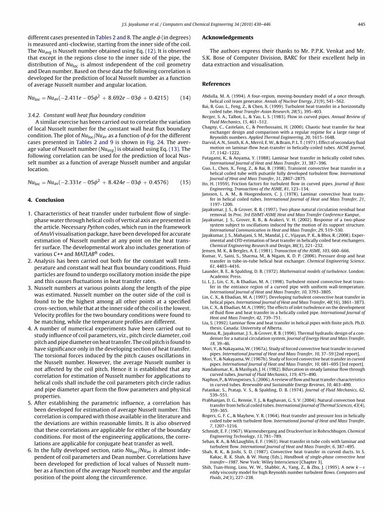
.4.2. Constant wall heat flux boundary conditionA similar exercise has been carried out to correlate the variation
f local Nusselt number for the constant wall heat flux boundaryondition. The plot of Nuloc/Nuav as a function of � for the differentases presented in Tables 2 and 9 is shown in Fig. 24. The aver-ge value of Nusselt number (Nuavg) is obtained using Eq. (13). Theollowing correlation can be used for the prediction of local Nus-elt number as a function of average Nusselt number and angularocation.
uloc = Nuav(−2.331e − 05�2 + 8.424e − 03� + 0.4576) (15)
. Conclusion
. Characteristics of heat transfer under turbulent flow of single-phase water through helical coils of vertical axis are presented inthe article. Necessary Python codes, which run in the frameworkof AnuVi visualisation package, have been developed for accurateestimation of Nusselt number at any point on the heat trans-fer surface. The developmental work also includes generation ofvarious C++ and MATLAB® codes.
. Analysis has been carried out both for the constant wall tem-perature and constant wall heat flux boundary conditions. Fluidparticles are found to undergo oscillatory motion inside the pipeand this causes fluctuations in heat transfer rates.
. Nusselt numbers at various points along the length of the pipewas estimated. Nusselt number on the outer side of the coil isfound to be the highest among all other points at a specifiedcross-section, while that at the inner side of the coil is the lowest.Velocity profiles for the two boundary conditions were found tobe matching, while the temperature profiles are different.
. A number of numerical experiments have been carried out tostudy influence of coil parameters, viz., pitch circle diameter, coilpitch and pipe diameter on heat transfer. The coil pitch is found tohave significance only in the developing section of heat transfer.The torsional forces induced by the pitch causes oscillations inthe Nusselt number. However, the average Nusselt number isnot affected by the coil pitch. Hence it is established that anycorrelation for estimation of Nusselt number for applications tohelical coils shall include the coil parameters pitch circle radiusand pipe diameter apart form the flow parameters and physicalproperties.
. After establishing the parametric influence, a correlation hasbeen developed for estimation of average Nusselt number. Thiscorrelation is compared with those available in the literature andthe deviations are within reasonable limits. It is also observedthat these correlations are applicable for either of the boundaryconditions. For most of the engineering applications, the corre-lations are applicable for conjugate heat transfer as well.
. In the fully developed section, ratio Nuloc/Nuav is almost inde-pendent of coil parameters and Dean number. Correlations havebeen developed for prediction of local values of Nusselt num-ber as a function of the average Nusselt number and the angularposition of the point along the circumference.
ical Engineering 34 (2010) 430–446 445
Acknowledgements
The authors express their thanks to Mr. P.P.K. Venkat and Mr.S.K. Bose of Computer Division, BARC for their excellent help indata extraction and visualisation.
References
Abdulla, M. A. (1994). A four-region, moving-boundary model of a once through,helical coil team generator. Annals of Nuclear Energy, 21(9), 541–562.
Bai, B, Guo, L., Feng, Z., & Chen, X. (1999). Turbulent heat transfer in a horizontallycoiled tube. Heat Transfer-Asian Research, 28(5), 395–403.
Berger, S. A., Talbot, L., & Yao, L. S. (1983). Flow in curved pipes. Annual Review ofFluid Mechanics, 15, 461–512.
Chagny, C., Castelain, C., & Peerhossaini, H. (2000). Chaotic heat transfer for heatexchanger design and comparison with a regular regime for a large range ofReynolds numbers. Applied Thermal Engineering, 20, 1615–1648.
Darvid, A. N., Smith, K. A., Merril, E. W., & Brain, P. L. T. (1971). Effect of secondary fluidmotion on laminar-flow heat-transfer in helically-coiled tubes. AICHE Journal,17, 1142–1222.
Futagami, K., & Aoyama, Y. (1988). Laminar heat transfer in helically coiled tubes.International Journal of Heat and Mass Transfer, 31, 387–396.
Guo, L., Chen, X., Feng, Z., & Bai, B. (1998). Transient convective heat transfer in ahelical coiled tube with pulsatile fully developed turbulent flow. InternationalJournal of Heat and Mass Transfer, 31, 2867–2875.
Ito, H. (1959). Friction factors for turbulent flow in curved pipes. Journal of BasicEngineering, Transactions of the ASME, 81, 123–134.
Janssen, L. A. M., & Hoogendoorn, C. J. (1978). Laminar convective heat trans-fer in helical coiled tubes. International Journal of Heat and Mass Transfer, 21,1197–1206.
Jayakumar, J. S., & Grover, R. B. (1997). Two phase natural circulation residual heatremoval. In Proc. 3rd ISHMT-ASME Heat and Mass Transfer Conference Kanpur,
Jayakumar, J. S., Grover, R. B., & Arakeri, V. H. (2002). Response of a two-phasesystem subject to oscillations induced by the motion of its support structure.International Communication in Heat and Mass Transfer, 29, 519–530.
Jayakumar, J. S., Mahajani, S. M., Mandal, J. C., Vijayan, P. K., & Bhoi, R. (2008). Exper-imental and CFD estimation of heat transfer in helically coiled heat exchangers.Chemical Engineering Research and Design, 86(3), 221–232.
Jensen, M. K., & Bergles, A. E. (1981). Transaction of the ASME, 103, 660–666.Kumar, V., Saini, S., Sharma, M., & Nigam, K. D. P. (2006). Pressure drop and heat
transfer in tube-in-tube helical heat exchanger. Chemical Engineering Science,61, 4403–4416.
Launder, B. E., & Spalding, D. B. (1972). Mathematical models of turbulence. London:Academic Press.
Li, L. J., Lin, C. X., & Ebadian, M. A. (1998). Turbulent mixed convective heat trans-fer in the entrance region of a curved pipe with uniform wall-temperature.International Journal of Heat and Mass Transfer, 10, 3793–3805.
Lin, C. X., & Ebadian, M. A. (1997). Developing turbulent convective heat transfer inhelical pipes. International Journal of Heat and Mass Transfer, 40(16), 3861–3873.
Lin, C. X., & Ebadian, M. A. (1999). The effects of inlet turbulence on the developmentof fluid flow and heat transfer in a helically coiled pipe. International Journal ofHeat and Mass Transfer, 42, 739–751.
Liu, S. (1992). Laminar flow and heat transfer in helical pipes with finite pitch. Ph.D.thesis. Canada: University of Alberta.
Manna, R., Jayakumar, J. S., & Grover, R. B. (1996). Thermal hydraulic design of a con-denser for a natural circulation system. Journal of Energy Heat and Mass Transfer,18, 39–46.
Mori, Y., & Nakayama, W. (1967a). Study of forced convective heat transfer in curvedpipes. International Journal of Heat and Mass Transfer, 10, 37–59 [2nd report].
Mori, Y., & Nakayama, W. (1967b). Study of forced convective heat transfer in curvedpipes. International Journal of Heat and Mass Transfer, 10, 681–695 [3rd report].
Nandakumar, K., & Masliyah, J. H. (1982). Bifurcation in steady laminar flow throughcurved tubes. Journal of Fluid Mechanics, 119, 475–490.
Naphon, P., & Wongwises, S. (2006). A review of flow and heat transfer characteristicsin curved tubes. Renewable and Sustainable Energy Reviews, 10, 463–490.
Patankar, S., Pratap, V. S., & Spalding, D. B. (1974). Journal of Fluid Mechanics, 62,539–551.
Prabhanjan, D. G., Rennie, T. J., & Raghavan, G. S. V. (2004). Natural convection heattransfer from helical coiled tubes. International Journal of Thermal Sciences, 43(4),359–365.
Rogers, G. F. C., & Mayhew, Y. R. (1964). Heat transfer and pressure loss in helicallycoiled tube with turbulent flow. International Journal of Heat and Mass Transfer,7, 1207–1216.
Schmidt, E. F. (1967). Warmeubergang and Druckverlust in Rohrschbugen. ChemicalEngineering Technology, 13, 781–789.
Seban, R. A., & McLaughlin, E. F. (1963). Heat transfer in tube coils with laminar andturbulent flow. International Journal of Heat and Mass Transfer, 6, 387–495.
Shah, R. K., & Joshi, S. D. (1987). Convective heat transfer in curved ducts. In S.Kakac, R. K. Shah, & W. Hung (Eds.), Handbook of single-phase convective heattransfer—1987. New York: Wiley Interscience [Chapter 3].
Shih, Tsan-Hsing, Liou, W. W., Shabbir, A., Yang, Z., & Zhu, J. (1995). A new k − εeddy viscosity model for high Reynolds number turbulent flows. Computers andFluids, 24(3), 227–238.

4 Chem
S
W
X
Yang, G., & Ebadian, M. A. (1996). Turbulent forced convection in a helicoidal pipe
46 J.S. Jayakumar et al. / Computers and
rinivasan, P. S., Nandapurkar, S. S., & Holland, F. A. (1970). Friction factor for coils.
Transactions of the Institution of Chemical Engineer, 48, T156–T161.ilson, E. E. (1915). A basis for rational design of heat transfer apparatus. Transac-tions of the ASME, 37, 47–82.
in, R. C., Awwad, A., Dong, Z. F., & Ebadin, M. A. (1996). An investigation and com-parative study of the pressure drop in air–water two-phase flow in verticalhelicoidal pipes. International Journal of Heat and Mass Transfer, 39(4), 735–743.
ical Engineering 34 (2010) 430–446
with substantial pitch. International Journal of Heat and Mass Transfer, 39(10),2015–2032.
Yildiz, C., Bicer, Y., & Pehlivan, D. (1997). Heat transfer and pressure drop in a heatexchanger with a helical pipe containing inside springs. Energy Conversion andManagement, 38(6), 619–624.