CFD Based Analysis and Parametric Study of a Novel Wind

Turbine Design: the Dual Vertical Axis Wind Turbine

Gabriel Naccache

A Thesis

In the Department

Of

Mechanical and Industrial Engineering

Presented in Partial Fulfillment of the Requirements

For the Degree of

Master of Applied Science (Mechanical Engineering) at

Concordia University

Montreal, Quebec, Canada

August 2016

© Gabriel Naccache, 2016

CONCORDIA UNIVERSITY

School of Graduate Studies

This is to certify that the thesis prepared

By: Gabriel Naccache

Entitled: CFD Based Analysis and Parametric Study of a Novel Wind Turbine Design: the

Dual Vertical Axis Wind Turbine

and submitted in partial fulfillment of the requirements for the degree of

Master of Applied Science (Mechanical Engineering)

complies with the regulation of the University and meets the accepted standards with respect to

originality and quality.

Signed by the final Examining Committee:

_______________________________ Chair

_______________________________ Examiner

_______________________________ Examiner

_______________________________ Supervisor

Approved by: _________________________________________________

MASc Program Director

Department of Mechanical and Industrial Engineering

____/____/2016 ________________________________________________

Dean of Faculty

Onur Kuzgunkaya

Liangzhu Wang

Wahid Ghaly

Marius Paraschivoiu

iii

ABSTRACT

CFD Based Analysis and Parametric Study of a Novel Wind Turbine Design:

the Dual Vertical Axis Wind Turbine

Gabriel Naccache

Small Vertical Axis Wind Turbines (VAWTs) are good candidates to extract energy from wind in

urban areas because they are easy to install, service and do not generate much noise; however, the

aerodynamic efficiency of small turbines is low. Here-in a new turbine, with high aerodynamic

efficiency, is proposed. The novel design is based on the classical H-Darrieus VAWT. VAWTs

produce the highest power when the blade chord is perpendicular to the incoming wind direction.

The basic idea behind the proposed turbine is to extend that said region of maximum power by

having the blades continue straight instead of following a circular path. This motion can be

performed if the blades turn along two axes; hence it was named Dual Vertical Axis Wind Turbine

(D-VAWT). The analysis of this new turbine is done through the use of Computational Fluid

Dynamics (CFD) with 2D and 3D simulations. While 2D is used to validate the methodology, 3D

is used to get an accurate estimate of the turbine performance. The analysis of a single blade is

performed and the turbine shows that a power coefficient of 0.4 can be achieved. So far, reaching

performance levels high enough to compete with the most efficient VAWTs. The D-VAWT is still

far from full optimization, but the analysis presented here shows the hidden potential and serves

as proof of concept. The study of the D-VAWT is concluded with a preliminary parametric study

of the turbine sensitivity to different incoming wind angles, turbine axes spacing, number of

blades, airfoil profile and blade mounting point.

Keywords: Wind Turbine, VAWT, Dual Axis, Innovative, Power Coefficient, CFD, Parametric

Study.

iv

ACKNOWLEDGMENTS

I would like to thank my thesis supervisor and mentor, Dr. Marius Paraschivoiu, for his

immeasurable support, guidance, and insight. The completion of this thesis would not have been

possible without his moral and educational support. I greatly appreciate his availability and

approachability as they were key in overcoming many obstacles faced during this thesis. He served

as an inspiration and allowed me to produce the best work possible. One could not wish for a better

supervisor.

I thank Le Fonds Quebecois de la Recherche sur la Nature et les Technologies (FQRNT) for the

funding of this research project. I would also like to thank the Concordia Institute for Water,

Energy and Sustainable Systems (CIWESS) and the Natural Sciences and Engineering Research

Council of Canada (NSERC) for partial funding of this project through the Collaborative Research

and Training Experience (CREATE) program.

My thanks go to Matin Komeili and my colleagues for their advice, their suggestions, and

contributing to an enjoyable working environment during my research. I am privileged to have

worked with you.

Special thanks to Hany Gomaa for his moral support and guidance during and before the start of

this thesis. I am very grateful to have met him as he helped me discover the joy of research and

academia.

I am also sincerely grateful to my close friends, Patrick Larin, Nelson David Hernández Blanco

and Abilash Krishnan, for their friendship and support.

Finally, I would like to thank my loving parents, Therese Khoury and Hugues Naccache, for their

unconditional love and support at my most challenging times. I am forever grateful to them. I

would like to dedicate my thesis to my family and my close friends.

v

TABLE OF CONTENTS

List of Figures .............................................................................................................................. viii

List of Tables ................................................................................................................................ xii

Nomenclature ............................................................................................................................... xiii

CHAPTER 1: Introduction ............................................................................................................. 1

1.1 Energy Production ............................................................................................................ 1

1.2 Wind Energy .................................................................................................................... 2

1.3 Wind Turbines .................................................................................................................. 5

1.4 Motivation ........................................................................................................................ 9

1.5 Objectives ....................................................................................................................... 11

1.6 Literature Review ........................................................................................................... 12

1.6.1 Methods of VAWT Analysis .................................................................................. 12

1.6.2 Current Research ..................................................................................................... 13

1.7 Thesis Outline ................................................................................................................ 18

CHAPTER 2: Methodology Considerations ................................................................................. 20

2.1 Governing Equations ...................................................................................................... 20

2.2 Turbulence Modelling .................................................................................................... 21

2.2.1 Spalart-Allmaras ..................................................................................................... 21

2.2.2 Shear-Stress Transport k-ω ..................................................................................... 23

2.2.3 Transition Shear-Stress Transport........................................................................... 23

2.3 Wall Treatment ............................................................................................................... 25

2.4 Original Turbine Geometry ............................................................................................ 26

2.5 Parameters for the D-VAWT ......................................................................................... 28

2.5.1 Swept Area .............................................................................................................. 28

2.5.2 Coefficient of Power ............................................................................................... 28

vi

2.5.3 Solidity .................................................................................................................... 30

2.5.4 Axis Eccentricity Factor ......................................................................................... 30

2.6 Theoretical Power Coefficient in Upstream Translational Region ................................ 31

2.7 Analysis Milestones ....................................................................................................... 32

CHAPTER 3: Methodology Validation in 2D .............................................................................. 34

3.1 Numerical Setup ............................................................................................................. 34

3.2 Initial Domain ................................................................................................................ 36

3.3 Investigation of Domain size .......................................................................................... 37

3.4 Different Motion Methodology ...................................................................................... 38

3.4.1 Motion Type 1......................................................................................................... 38

3.4.2 Motion Type 2......................................................................................................... 40

3.4.1 Motion Type 3......................................................................................................... 40

3.4.2 Results and Discussion ........................................................................................... 43

3.5 Mesh Convergence Study using SST k-ω Model with 𝒚 +~ 1 ...................................... 44

3.5.1 Meshes .................................................................................................................... 45

3.5.2 Results and Discussion ........................................................................................... 49

3.6 Turbulence Model Study ................................................................................................ 50

3.7 Airfoil Validation with Experimental Results ................................................................ 52

3.7.1 Domain and Mesh ................................................................................................... 52

3.7.2 Results and Discussion ........................................................................................... 53

3.8 Summary and Conclusions ............................................................................................. 56

CHAPTER 4: 3D Investigation .................................................................................................... 58

4.1 Domain ........................................................................................................................... 58

4.2 Mesh ............................................................................................................................... 59

4.3 Numerical Setup ............................................................................................................. 63

4.4 Results and Discussion ................................................................................................... 63

vii

4.5 Comparison of 2D and 3D Results ................................................................................. 69

4.6 Discussion of D-VAWT Performance ........................................................................... 70

CHAPTER 5: 2D Parametric Study .............................................................................................. 72

5.1 Introduction to Parametric Study ................................................................................... 72

5.2 TSR Study of Original Turbine ...................................................................................... 73

5.3 Incident Wind Angle ...................................................................................................... 76

5.4 Axis Eccentricity Factor (AEF) ...................................................................................... 82

5.5 Multi-Blade Turbine Analysis ........................................................................................ 86

5.6 High Lift-to-Drag Airfoil ............................................................................................... 90

5.7 Blade Mounting Point .................................................................................................... 92

5.8 Summary and Discussion of Parametric Study .............................................................. 94

CHAPTER 6: Conclusion ............................................................................................................. 95

6.1 Summary ........................................................................................................................ 95

6.2 Contributions .................................................................................................................. 96

6.3 Future Work ................................................................................................................... 96

6.3.1 Future Work Summary ........................................................................................... 97

References ..................................................................................................................................... 98

viii

LIST OF FIGURES

Figure 1.1: World Total Primary Energy Supply from 1971 to 2013 by fuel (Mtoe). 2Peat and Oil

Shale are Aggregated with Coal. 3Includes Geothermal, Solar, Wind, Heat, etc. [1] .................... 2

Figure 1.2: Canada’s Primary Energy Production by Source in 2013. “Other Renewables” Includes

Wind, Solar, Wood/Wood Waste, Biofuels and Municipal Waste [2] ........................................... 2

Figure 1.3: Global Cumulative Installed Wind Capacity 2000-2015 [3] ........................................ 3

Figure 1.4: Cumulative and Annual Installed Capacity in Canada [2] ........................................... 3

Figure 1.5: Example of Large Scale Wind Turbines (a) Siemens G2 2.3MW [5], (b) Éole Rotor

Darrieus 4.3MW [6] ........................................................................................................................ 4

Figure 1.6: Examples of Small Scale Wind Turbines (a) Helix Wind 5kW Savonius [7], (b) Quiet

Revolution 7.5kW [8], (c) WHI 70kW [9] ..................................................................................... 5

Figure 1.7: Global Installed Energy Capacity and Units [4] .......................................................... 5

Figure 1.8: Main Types of Wind Turbines [10, 11] ........................................................................ 6

Figure 1.9: Different Darrieus Wind Turbines [12] ........................................................................ 6

Figure 1.10: Power Coefficients for Different Rotor Designs [13, 14] ......................................... 7

Figure 1.11: Top view of a typical H-Darrieus VAWT with Velocity Vectors and Forces, Where

θ is the Azimuthal Angle, U∞ is the Free Stream Velocity, Vblade is The Blade Velocity, Urelative is

The Relative Velocity Seen by the Blade, α is the Effective Angle of Attack, D is the Drag Force,

And L is the Lift Force .................................................................................................................. 10

Figure 1.12: Torque Variation Versus Azimuthal angle for 2D Simulation H-Darrieus Turbine (a)

TSR = 2 and (b) TSR =3 [16] ....................................................................................................... 10

Figure 1.13: Example of D-VAWT (a) Top View (b) 3D CAD Model ....................................... 11

Figure 1.14: Summary of Methods for VAWT Analysis ............................................................. 13

Figure 1.15: Turbulence Modeling Behavior at High TSR (λ=4.25) (Left) and Low TSR (λ=2.55)

(Right) [31] ................................................................................................................................... 16

Figure 2.1: Law of the Wall [55] .................................................................................................. 25

Figure 2.2: Top View of a D-VAWT Path ................................................................................... 27

Figure 2.3: Steps for Coefficient of Power Calculation (a) Force Based, (b) Torque Based ....... 29

ix

Figure 2.4: Instantaneous Coefficient of Power Curve Based on the Combination of both the Force

and Torque Based Methods .......................................................................................................... 30

Figure 2.5: Milestones for the CFD Analysis of the D-VAWT .................................................... 33

Figure 3.1: Initial Domain with Boundary Conditions ................................................................. 36

Figure 3.2: View of the Rotating Domain and Blade Refinement Region ................................... 36

Figure 3.3: Instantaneous CP vs. Normalized Time of the 10th Cycle for Different Domain Sizes

....................................................................................................................................................... 38

Figure 3.4: Type 1 Motion Illustration ......................................................................................... 39

Figure 3.5: Mesh Used for Type 1 and 2 Motions ........................................................................ 39

Figure 3.6: Rotating Domain Mesh for Type 1 and 2 Motions .................................................... 40

Figure 3.7: Type 2 Motion Illustration ......................................................................................... 41

Figure 3.8: Type 3 Motion Illustration ......................................................................................... 41

Figure 3.9: Overview of Mesh Used for Type 3 Motion .............................................................. 42

Figure 3.10: Deforming Domain Mesh View for Type 3 Motion ................................................ 42

Figure 3.11: Dynamic Domain Mesh View for Type 3 Motion ................................................... 43

Figure 3.12: Instantaneous CP versus Normalized Time of the 10th Cycle for Motion Types .... 44

Figure 3.13: Rotating Domain Mesh View for Mesh 1 ................................................................ 46

Figure 3.14: Refinement Region Mesh Around Blade for Mesh 1 ............................................... 47

Figure 3.15: Boundary Layer Views for Mesh 1 at Leading Edge (Top), Mid-Chord (Middle), and

Trailing Edge (Bottom) ................................................................................................................. 47

Figure 3.16: Rotating Domain Mesh View for Mesh 2 ................................................................ 48

Figure 3.17: Refinement Region Mesh Around Blade for Mesh 2 ............................................... 48

Figure 3.18: Boundary Layer View for Mesh 3 ............................................................................ 48

Figure 3.19: Average Cycle CP Convergence Plot for Mesh 1 ..................................................... 49

Figure 3.20: Instantaneous CP versus Normalized Time at 15th Cycle for Mesh and Time

Convergence Study Cases ............................................................................................................. 50

Figure 3.21: Instantaneous CP Plots of the 15th cycle for the Turbulence Model Study Using Mesh

1 at TSR=4.5 ................................................................................................................................. 51

Figure 3.22: Overview of (a) Domain (b) Mesh, for the Experimental Case Simulation ............. 53

Figure 3.23: Mesh Near Blade for (a) 𝑦 +~ 30 (b) 𝑦 +~ 1 .......................................................... 53

Figure 3.24: Coefficient of Lift vs Angle of Attack ..................................................................... 54

x

Figure 3.25: Coefficient of Drag vs Angle of Attack ................................................................... 54

Figure 3.26: Ratio of Coefficient of Lift to Coefficient of Drag vs Angle of Attack ................... 55

Figure 3.27: Coefficient of Lift vs Coefficient of Drag ................................................................ 55

Figure 4.1: 3D Domain for D-VAWT with AR=5 ....................................................................... 58

Figure 4.2: Rotating Domain Mesh at Symmetry Plane for AR=5 and 𝑦 +~ 30 ......................... 60

Figure 4.3: Refinement Region Mesh at Symmetry Plane for AR=5 and 𝑦 +~ 30 ...................... 61

Figure 4.4: Boundary Layer Mesh View at Symmetry Plane for AR=5 and 𝑦 +~ 30 ................. 61

Figure 4.5: Cross Section of Mesh Around the Blade AR=5 and 𝑦 +~ 30 .................................. 61

Figure 4.6: Refinement Region Mesh at Symmetry Plane for AR=5 and 𝑦 +~ 1 ........................ 62

Figure 4.7: Boundary Layer Mesh View at Symmetry Plane for AR=5 and 𝑦 +~ 1 ................... 62

Figure 4.8: Cross Section of Mesh Around the Blade for AR=5 and 𝑦 +~ 1 .............................. 62

Figure 4.9: Boundary Conditions for 3D Domains ....................................................................... 63

Figure 4.10: Average CP per Cycle Convergence for 3D Simulations ......................................... 64

Figure 4.11: Instantaneous CP Plots of the Last Cycle for 3D Simulations .................................. 65

Figure 4.12: Normalized Velocity Deficit ( 𝑈∞ − 𝑈𝑈∞) Plots on a Plane of Half a Chord Away

in the Span-Wise Direction from the Symmetry Plane at t/T=0.68 for Cases (a) SA Strain/Vorticity

(𝑦 +~ 30) with AR =5, (b) SA Strain/Vorticity (𝑦 +~ 30) with AR =15, (c) SST k-ω (𝑦 +~ 1) with

AR =5, and (d) SST k-ω (𝑦 +~ 1) with AR =15 .......................................................................... 67

Figure 4.13: Static Pressure Contour on Half of the Blade Surface for SST k-ω (𝑦 +~ 1) Model at

t/T=0.33 for (a) AR = 15 (b) AR = 5 ............................................................................................ 68

Figure 4.14: Turbulent Viscosity Ratio ( 𝜈𝑡𝜈) Plots on a Plane of Half a Chord Away in the Span-

Wise Direction from the Symmetry Plane at t/T=0.33 for Cases (a) SA Strain/Vorticity (𝑦 +~ 30)

with AR =5, (b) SA Strain/Vorticity (𝑦 +~ 30) with AR =15 and (c) SST k-ω (𝑦 +~ 1) with AR

=5, and (d) SST k-ω (𝑦 +~ 1) with AR =15 ................................................................................. 68

Figure 4.15: Comparing Instantaneous CP for 2D and 3D with AR =5 and 15 Using the SST k-ω

Model (𝑦 +~ 1) ............................................................................................................................. 69

Figure 5.1: Instantaneous Blade Angle of Attack for Darrieus Type VAWT vs Azimuthal Angle

for Different TSRs ........................................................................................................................ 73

Figure 5.2: Average Power Coefficient Convergence per Cycle for Different TSR values for

AEF=4 ........................................................................................................................................... 74

Figure 5.3: Average CP per Cycle vs TSR for AEF= 4 with Quadratic Curve Fitting ................. 74

xi

Figure 5.4: Instantaneous CP for Different TSR Values at AEF =4 ............................................. 75

Figure 5.5: Incident Wind Angle Convention ............................................................................... 76

Figure 5.6: Average CP for Different TSRs with Different Incoming Incident Wind Angles with

Quadratic Curve Fitting ................................................................................................................ 77

Figure 5.7: Peak CP for Each Incident Wind Angle ...................................................................... 78

Figure 5.8: Instantaneous CP for Different TSR Values for φ = -20o ........................................... 79

Figure 5.9: Instantaneous CP for Different TSR Values for φ = -40o ........................................... 79

Figure 5.10: Instantaneous CP for Different TSR Values for φ = -60o ......................................... 79

Figure 5.11: Instantaneous CP for Different TSR Values for φ = +20o ........................................ 80

Figure 5.12: Instantaneous CP for Different TSR Values for φ = +40o ........................................ 80

Figure 5.13: Instantaneous CP for Different TSR Values for φ = +60o ........................................ 80

Figure 5.14: Percent Time Translating vs AEF ............................................................................ 82

Figure 5.15: Average CP per Cycle vs TSR for AEF Study with Quadratic Curve Fitting ......... 83

Figure 5.16: Instantaneous CP for Different TSRs with AEF = 8 ................................................ 85

Figure 5.17: Instantaneous CP for Different TSRs with AEF = 12 .............................................. 85

Figure 5.18: View of Deforming Domain at (a) t/T = 0 and (b) t/T = 0.36 .................................. 86

Figure 5.19: Close View of Mesh Around Blades at t/T = 0.36 ................................................... 87

Figure 5.20: Average Power Coefficient Convergence per Cycle for Different TSR values for Two

Bladed Turbine .............................................................................................................................. 87

Figure 5.21: Average CP per Cycle vs TSR for a Single and Two Bladed Turbine ..................... 88

Figure 5.22: Instantaneous CP of Blade 1 of the Two Bladed Turbine ........................................ 89

Figure 5.23: Total Instantaneous CP for Two Bladed Turbine ..................................................... 89

Figure 5.24: Comparison of Instantaneous CP at Best TSR for the Single and Two Blade Turbines

....................................................................................................................................................... 90

Figure 5.25: S1223 and NACA 0018 Airfoil Profile .................................................................... 91

Figure 5.26: Average CP per Cycle vs TSR for Different Blade Airfoil Profiles ........................ 91

Figure 5.27: Instantaneous CP for Different TSRs for the S1223 Airfoil .................................... 92

Figure 5.28: Average CP per Cycle vs TSR for Different Blade Mounting Points (MP) ............. 93

Figure 5.29: Instantaneous CP for Different TSRs for the Blade Mounting Point at Half Chord 93

xii

LIST OF TABLES

Table 1.1: Summary of the Most Important Differences between the H-Rotor Darrieus, Rotor

Darrieus and HAWT [11] ............................................................................................................... 8

Table 1.2: Comparative Analysis of the Literature Settings for 2D Unsteady Simulations of

Darrieus Type VAWTs [32] ......................................................................................................... 16

Table 2.1: D-VAWT Geometrical Characteristics ........................................................................ 27

Table 2.2: Summary of Theoretical Results ................................................................................. 32

Table 3.1: Results Summary for Domain Size Study ................................................................... 37

Table 3.2: Comparison of Results for Different Motion Types .................................................... 43

Table 3.3: Details of Each Mesh Used for Mesh Study ................................................................ 46

Table 3.4: Mesh and Time Convergence Study Results ............................................................... 49

Table 3.5: Results for the Turbulence Model Study Using Mesh 1 at TSR =4.5 ......................... 51

Table 3.6: Percent Error for Airfoil Case Study (Positive is Over Prediction and Negative is Under

Prediction) ..................................................................................................................................... 56

Table 4.1: 3D Domain Characteristics .......................................................................................... 59

Table 4.2: 3D Meshes Details ....................................................................................................... 60

Table 4.3: CP Results Summary for 3D Simulations .................................................................... 64

Table 5.1: Summary of Peak CP for the Incident Wind Angle Study ........................................... 78

Table 5.2: Summary of Average CP per Section at TSR = 5.5 for φ =0° and +20° ....................... 81

Table 5.3: Summary of AEF Study for Peak Performance ........................................................... 83

Table 5.4: Summary of AEF Study for Peak and 90% of Peak Performances Using Curve Fitted

Data ............................................................................................................................................... 84

xiii

NOMENCLATURE

𝜆 Tip Speed Ratio (TSR)

𝜔 Angular Velocity [rad/s]

𝑅 Turbine Radius [m]

𝑈∞ Free Stream Velocity [m/s]

𝐶𝑃 Coefficient of Power

𝑃 Total Extracted Power [W]

𝑃𝑎 Available Power in Incoming Wind [W]

𝜌 Fluid Density [kg/m3]

𝐴 Turbine Swept Area [m2]

𝜃 Azimuthal Angle [deg]

𝐿 Distance Between Axes of Rotation [m]

𝐶 Chord [m]

𝐷 Turbine Diameter [m]

ℎ Blade Height [m]

𝐴𝑅 Blade Aspect Ratio [m]

𝜑 Incoming Incident Wind Direction Angle [deg]

𝑇𝑅𝑜𝑡𝑎𝑡𝑖𝑛𝑔 Sum of the Torque Produced When the Blade is Rotating for a Single

Cycle [N.m]

xiv

𝐹𝑇𝑟𝑎𝑛𝑠𝑙𝑎𝑡𝑖𝑛𝑔 Sum of the Tangential Force Produced When the Blade is Translating for

a Single Cycle [N]

𝑉𝑏𝑙𝑎𝑑𝑒 Blade Velocity [m/s]

𝐶𝑃, 𝑇𝑜𝑟𝑞𝑢𝑒 Coefficient of Power for the Rotating Sections

𝐶𝑃, 𝐹𝑜𝑟𝑐𝑒 Coefficient of Power for the Translational Sections

𝜎 Solidity

𝑁𝑏 Number of Blades

𝜀 Axis Eccentricity Factor (AEF)

𝐴𝐴𝐹 Airfoil Planform Area [m2]

Re Reynolds Number Based On Blade Velocity

𝐶𝐿 Coefficient of Lift

𝐶𝐷 Coefficient of Drag

𝛥𝑡 Time Step Size [ms]

𝑇 Period [s]

𝜇 Dynamic Viscosity [Kg/m.s]

𝜈𝑡 Turbulent Kinematic Viscosity [m2/s]

𝜈 Kinematic Viscosity [m2/s]

𝛼 Angle of Attack [deg]

1

CHAPTER 1: INTRODUCTION

1.1 Energy Production

Global energy consumption has been exponentially increasing over the last few decades, largely

due to the increase in energy demand from developing and developed countries related to the

growth in global population and the increase in personal demand. A country’s economic, social

and technological growth are closely tied to the availability of energy. This is especially true for

developing countries. Energy has undoubtedly become a basic human need in this modern day era

and will continue to be for the distant future. The main consumers of energy are the residential,

commercial/institutional, industrial, and transportation sectors.

Figure 1.1 shows the growth of energy supply from 1971 to 2013 as well as the breakdown of

energy production by source type as reported by the International Energy Agency (IEA) [1]. From

the same figure, one can see that from 1971 until 2013, the bigger portion of the world’s energy is

still produced from fossils fuels such as coal, petroleum/oil and natural gas. Though energy sources

such as nuclear, hydro and renewables have been growing, they still represent a fraction of the

total supply. Figure 1.2 shows the breakdown of energy in Canada, published by the Natural

Resources Canada (NRCan) [2]. Similarly to before, nearly 90% of the total energy produced is

from fossil fuels. As one might know, these sources of energy are finite and more importantly,

they produce large amounts of greenhouse gases (GHGs), which in turn damage our environment

and increase the effects of climate change.

The need for a sustainable and efficient source of renewable energy is highly in demand and

satisfying this need has been an objective for decades. There are a number of available renewable

energy sources to tap into, such as solar, wind, geothermal, hydro, biomass and tidal. There has

been increased interest in these cleaner and renewable sources of energy as they reduce the reliance

on those other finite sources of energy as well greatly reduce the effects of GHGs to help fight

climate change.

2

Figure 1.1: World Total Primary Energy Supply from 1971 to 2013 by fuel (Mtoe). 2Peat and Oil Shale

are Aggregated with Coal. 3Includes Geothermal, Solar, Wind, Heat, etc. [1]

Figure 1.2: Canada’s Primary Energy Production by Source in 2013. “Other Renewables” Includes

Wind, Solar, Wood/Wood Waste, Biofuels and Municipal Waste [2]

1.2 Wind Energy

Wind energy has shown great potential as a sustainable solution and its production has grown

tremendously in recent years. Figure 1.3 shows the growth of wind energy capacity on a global

scale as published by the Global Wind Energy Council (GWEC) [3], while Figure 1.4 shows the

3

wind energy capacity in Canada. Wind energy has been used as both a complementary source of

energy as well as a substitute for other sources of energy. The numerous types of wind turbines in

sizes and applications make it a very flexible source of energy. The most common way of

extracting energy from the wind is through wind turbines. The only stage in which wind turbines

pollute the environment is before the installation stage. Once the turbines are installed, they

produce negligible amounts of GHGs for the rest of their life cycles. Since their first use, wind

turbines have gone through incredible technological advancements and even until now, there is

still plenty of room for improvements and development. Wind turbines have gotten more efficient

and much bigger since they were first invented thanks to advancements in aerodynamic, structural

and material design.

Figure 1.3: Global Cumulative Installed Wind Capacity 2000-2015 [3]

Figure 1.4: Cumulative and Annual Installed Capacity in Canada [2]

4

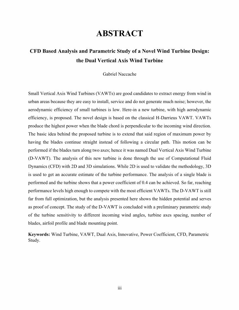
Wind turbines of large scale are used for onshore and offshore farms while the small scale turbines

are used for urban applications. Large scale turbines are the ones that can typically produce 100kW

and above, shown in Figure 1.5, while small scale turbines, shown in Figure 1.6 produce below

that threshold. It should be noted that whether a turbine is considered large or small for

accreditation purposes, the turbine swept area is used instead as criterion. So far, the large wind

turbines have been favored as they were typically more efficient and produced significantly higher

amounts of power. However, recent advancements in small scale wind turbines have made them

more attractive, especially since distributed energy production is quite an attractive concept, as it

is a much cheaper solution because power can be produced locally or near where it would be

consumed. Therefore, typical problems faced with large scale turbines such as transportation,

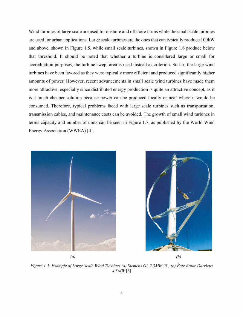
transmission cables, and maintenance costs can be avoided. The growth of small wind turbines in

terms capacity and number of units can be seen in Figure 1.7, as published by the World Wind

Energy Association (WWEA) [4].

(a) (b)

Figure 1.5: Example of Large Scale Wind Turbines (a) Siemens G2 2.3MW [5], (b) Éole Rotor Darrieus

4.3MW [6]

5

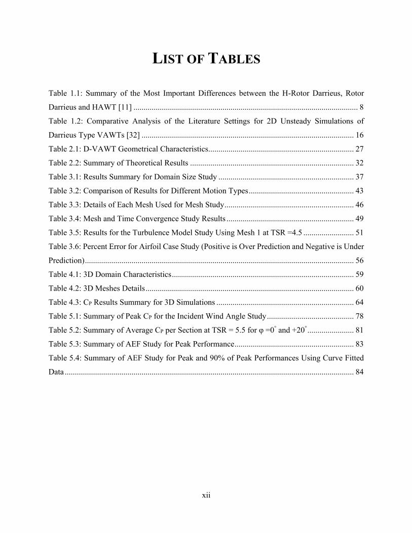
(a) (b) (c)

Figure 1.6: Examples of Small Scale Wind Turbines (a) Helix Wind 5kW Savonius [7], (b) Quiet

Revolution 7.5kW [8], (c) WHI 70kW [9]

(a) (b)

Figure 1.7: Global Installed Energy Capacity and Units [4]

1.3 Wind Turbines

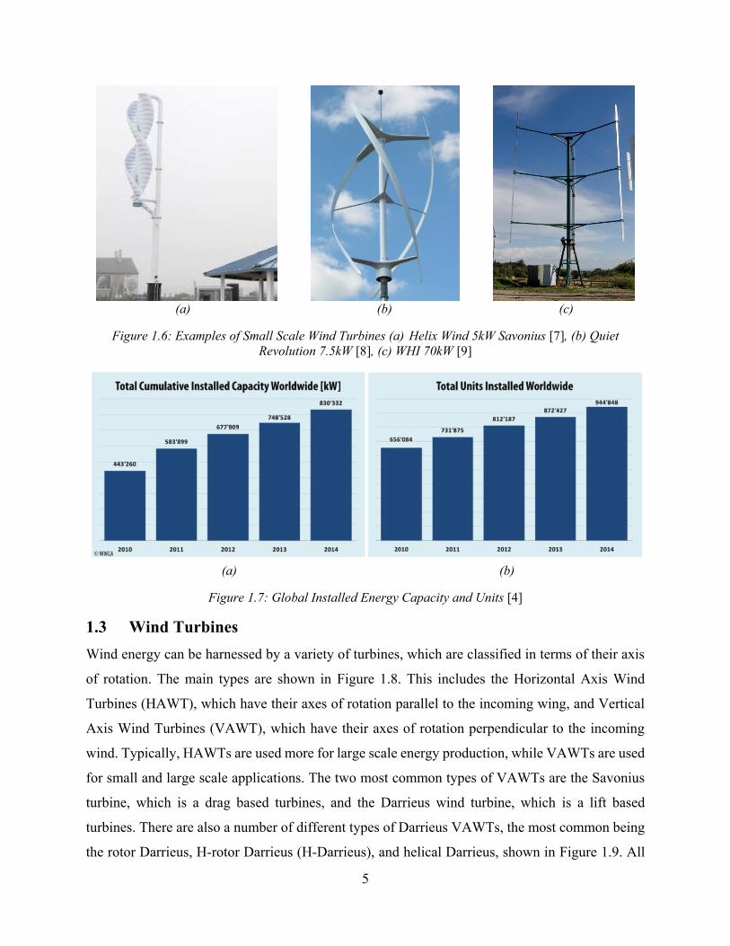
Wind energy can be harnessed by a variety of turbines, which are classified in terms of their axis

of rotation. The main types are shown in Figure 1.8. This includes the Horizontal Axis Wind

Turbines (HAWT), which have their axes of rotation parallel to the incoming wing, and Vertical

Axis Wind Turbines (VAWT), which have their axes of rotation perpendicular to the incoming

wind. Typically, HAWTs are used more for large scale energy production, while VAWTs are used

for small and large scale applications. The two most common types of VAWTs are the Savonius

turbine, which is a drag based turbines, and the Darrieus wind turbine, which is a lift based

turbines. There are also a number of different types of Darrieus VAWTs, the most common being

the rotor Darrieus, H-rotor Darrieus (H-Darrieus), and helical Darrieus, shown in Figure 1.9. All

6

the Darrieus type turbines have an airfoil profile for their blade cross-section, but differ in their

blade shape. An example of a HAWT, rotor Darrieus VAWT, Savonius VAWT, Helicoidale

VAWT and H-rotor VAWT can be seen in Figure 1.5 (a) and (b) and Figure 1.6 (a), (b) and (c),

respectively.

Figure 1.8: Main Types of Wind Turbines [10, 11]

Figure 1.9: Different Darrieus Wind Turbines [12]

The following two dimensionless parameters are commonly used to describe the performance and

operating condition of a VAWT. The first is the Tip Speed Ratio (TSR), which is the ratio of the

blade speed at the tip to the incoming wind speed.

HAWT Savonius

VAWT Darrieus

VAWT

Rotor Darrieus H-Rotor Darrieus Rotor Helicoidale

7

𝜆 = 𝑇𝑆𝑅 =𝜔𝑅

𝑈∞ (1.1)

Where 𝜔 is the angular velocity of the turbine, R is the radius of the turbine, and 𝑈∞ is the free

stream velocity. The second is the Coefficient of Power (CP) which is the ratio of extracted power

to the available power (available kinetic energy per unit time) in the incoming wind. The power

coefficient is a measure of the aerodynamic efficiency of turbines.

𝐶𝑃 = 𝑃𝑜𝑤𝑒𝑟 𝐶𝑜𝑒𝑓𝑓𝑖𝑐𝑖𝑒𝑛𝑡 =𝑃

12𝜌𝑈∞

3𝐴 (1.2)

Where P is the extracted power from the turbine, 𝜌 is the fluid density, and A is the turbine swept

area.

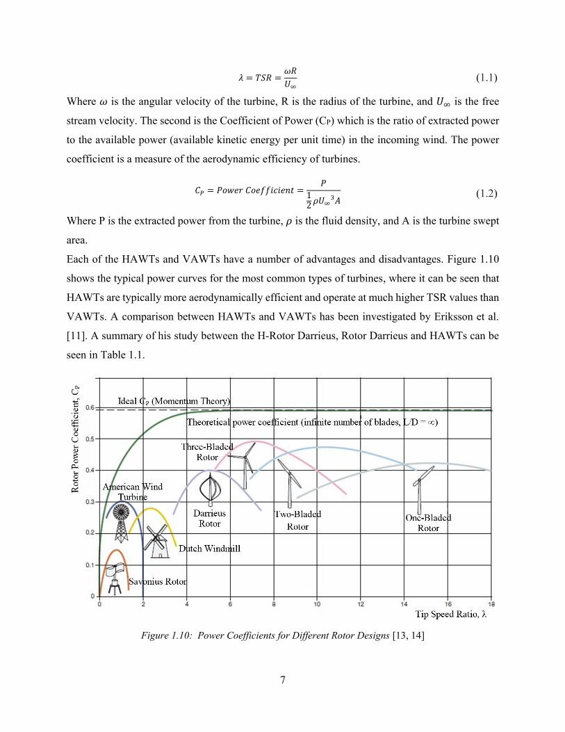
Each of the HAWTs and VAWTs have a number of advantages and disadvantages. Figure 1.10

shows the typical power curves for the most common types of turbines, where it can be seen that

HAWTs are typically more aerodynamically efficient and operate at much higher TSR values than

VAWTs. A comparison between HAWTs and VAWTs has been investigated by Eriksson et al.

[11]. A summary of his study between the H-Rotor Darrieus, Rotor Darrieus and HAWTs can be

seen in Table 1.1.

Figure 1.10: Power Coefficients for Different Rotor Designs [13, 14]

8

Table 1.1: Summary of the Most Important Differences between the H-Rotor Darrieus, Rotor Darrieus

and HAWT [11]

HAWTs are among the most efficient turbines and can be more easily scaled up in size for higher

amounts of energy production; however, they are highly dependent on the wind direction, needing

to face the wind for optimal performance. An added yawing and pitching mechanism can be added

to increase their flexibility at the cost of higher complexity and financial cost. The manufacturing

of their blades is more expensive than VAWTs’ since the blade cross sectional profile varies along

the span, while a number of VAWTs have the same blade profile along the span. Because HAWTs’

gearboxes, generators and other mechanical components are at the top of the tower, their

maintenance is more difficult, expensive and dangerous. They are also known to be quite noisy

since they operate at high tip speed ratios and since the blades are placed at a large height, the

sound produced can propagate more easily. Also, another disadvantage from the enormous height

of the tower is the flicker of the blades’ shadow, which have been known to cause problems for

people staying in affected areas. Thus, theses turbines have to be placed in remote areas, where

additional costs are incurred related to transportation and road building costs.

VAWTs address a number of these disadvantages. They produce much less noise since their

operating speeds are lower than HAWTs. Their maintenance is simpler since all components (the

gearbox, generator, etc.) are placed on the ground. They typically do not require a yaw control

mechanism as their performance is independent of the incoming wind direction. Also, because

they have smaller wakes than HAWTs, they can be packed quite closely together, resulting in

higher turbine density per unit area. However, VAWTs are generally less aerodynamically

9

efficient than HAWTs. They are structurally more challenging to design since the loads on the

blade continuously change throughout the turbine rotation. The constant change in the blade

incident angle puts them more at risk of failure due of fatigue loads. Also, most VAWTs lack self-

starting capabilities, except for the Savonius turbine, but it has lower aerodynamic efficiency than

other VAWTs.

1.4 Motivation

Small VAWTs are good candidates for urban areas because they are easy to install, service and do

not generate much noise. Nevertheless, the wind speed in urban areas is low, leading to low power

generation for a given area. To address this weakness a new type of wind turbine is investigated

in an attempt to improve the aerodynamic efficiency of small wind turbines. VAWTs produce the

highest power when the blade is near perpendicular to the incoming wind direction. This result is

confirmed by Paraschivoiu [15]. Figure 1.11 shows the top view of an H-Darrieus turbine as well

as the convention for the azimuthal angle, θ, which defines the position of the blade. The maximum

power is produced when the blade is at θ ~ 90°, which is confirmed by looking at Figure 1.12,

which is the torque graph vs azimuthal angle for an H-Darrieus turbine obtained from

Computational Fluid Dynamics (CFD) simulations performed by Zadeh et al. [16]. At this position,

the blade sees an effective flow angle and flow velocity that is optimal. Note that the flow reaching

the blade is the vector sum of the incoming wind and blade velocities. An example of the velocity

vectors seen by the blade is shown Figure 1.11 for a Darrieus turbine with multiple blades at three

positions.

10

Figure 1.11: Top view of a typical H-Darrieus VAWT with Velocity Vectors and Forces, Where θ is the

Azimuthal Angle, U∞ is the Free Stream Velocity, Vblade is The Blade Velocity, Urelative is The Relative

Velocity Seen by the Blade, α is the Effective Angle of Attack, D is the Drag Force, And L is the Lift Force

(a) (b)

Figure 1.12: Torque Variation Versus Azimuthal angle for 2D Simulation H-Darrieus Turbine (a) TSR =

2 and (b) TSR =3 [16]

11

The new turbine concept, with a similar blade shape as the H-Darrieus, would utilize the location

of maximum power and have it extended by letting the blades continue straight in an attempt to

increase the overall aerodynamic efficiency of the turbine. This motion can be achieved if the

blades turn around two axes, hence it was named Dual Vertical Axis Wind Turbine (D-VAWT).

Figure 1.13 shows a top view of the turbine and a 3D CAD model to give a better idea of the

geometry and mechanism of the D-VAWT. It should be noted that the mechanism will not be

present in any simulations. It is shown here for illustration purposes only.

(a) (b)

Figure 1.13: Example of D-VAWT (a) Top View (b) 3D CAD Model

1.5 Objectives

Investigate the feasibility of the D-VAWT design for a single blade analysis using ANSYS

Fluent 14.5 [17].

Develop methodology to specify the motion of a D-VAWT blade as conventional methods

for VAWT analysis would not directly apply for the current analysis.

Perform a domain size, mesh convergence, turbulence model and 𝑦+ study in 2D to

determine the most appropriate setup for this analysis as well as find the cheapest mesh

possible to be used for the 3D analysis.

12

Based on the 2D methodology investigation, 3D simulations are to be performed to get a

more accurate prediction of the turbine performance as 2D analysis has a tendency to

overestimate power coefficient values as 3D losses are not accounted for.

Perform a preliminary parametric study of the D-VAWT in 2D as it is possible to use the

predicted behavior and trends for future designs of the D-VAWT. Investigation of the TSR

behavior of the original turbine as well as the turbine sensitivity to different incoming wind

angles, turbine axes spacing, number of blades, airfoil profile and blade mounting point are

to be performed.

1.6 Literature Review

In this section, the possible methods of analyzing a VAWT will be outlined followed by a detailed

review of current research with a focus on CFD modeling as it will be the tool of analysis in this

thesis.

1.6.1 Methods of VAWT Analysis

There are various methods to study the performance of a VAWT. The main two categories are to

use either experimental or numerical methods. The methods are summarized in Figure 1.14.

Experimental analysis is done in wind tunnels, while numerical analysis is done through modeling

of fluid phenomenon. Numerical models can be broken down to Computational Aerodynamics and

Computational Fluid Dynamics (CFD). Aerodynamic models are significantly faster than CFD

ones, but lack accuracy in predicting VAWT performance, especially when the turbine operates at

low TSRs. Aerodynamic models were previously the most common modelling method as the

resources needed to perform CFD simulation were too expensive; however with current

advancements in computational power, CFD simulations have become much more attractive. For

CFD simulations, the Navier-Stokes equations are discretized and solved, providing much more

accurate results, but the drawback is higher computation cost and time. Even in CFD, there are

various methods of modeling the flow; the most common for engineering applications is the

Reynolds Averaged Navier-Stokes (RANS) models with turbulence modeling as it is able to

predict VAWTs’ performance with satisfactory accuracy. This will be the analysis method of

choice for this thesis as it provides enough accuracy with reasonable computational costs. The

other more accurate CFD models are the Eddy Simulations, where turbulence is now resolved and

only eddies below the grid size are modeled. Though Eddy Simulations are more accurate than

13

RANS models, they require significantly higher computational cost. The Detached Eddy

Simulation (DES) is a hybrid model of the Large Eddy Simulation (LES) and the RANS models.

Finally, the most accurate and computationally expensive is the Direct Numerical Simulation

(DNS), where the Navier-Stokes equations are completely resolved without any modeling which

is the reason it requires tremendous computational cost as the mesh and time step needed are

extremely fine. Xin et al. [18] provide more details on most of the methods presented here with

relevant research done on Darrieus VAWTs. It should be noted that not all RANS models that exist

have been presented here, but only the commonly used ones for VAWT analysis.

Figure 1.14: Summary of Methods for VAWT Analysis

1.6.2 Current Research

This section focuses on presenting recent research mainly done on VAWTs using CFD, which will

constitute the basis of the methodology used during this thesis project. Though more focus will be

on the H-Rotor Darrieus (H-Darrieus), as the turbine studied in this thesis resembles it the most

Methods of VAWT

Analysis

ExperimentalWind Tunnel Experiments

Particle Image Velocimetry

Numerical

Computational Aerodynamics

Blade Element Momentum (BEM)

Models

Single Streamtube Model

Multiple Streamtube Model

Double-Mutiple Streamtube ModelVortex Model

Cascade Model

Computational Fluid Dynamics

(CFD)

Reynolds-Averaged-Navier-Stokes (RANS)

with Turbulence Modeling

One-Equation Spalart-Allmaras

Two-Equation k-Epsilon

Two-Equation k-Omega

Two-Equation SST k-Omega

Four-Equation Transition SST

Eddy Simulation Models

Large Eddy Simulation (LES)

Detached Eddy Simulation (DES)

Direct Numerical Simulation (DNS)

14

from a geometrical point of view. Interesting and relevant work on new innovative concept

turbines will also be presented.

1.6.2.1 New Turbine Concepts

Using a similar idea of extending the maximum power region of a VAWT, Ponta el al. [19, 20]

analyzed a Variable Geometry Oval-Trajectory (VGOT) Darrieus wind turbine using the double-

multiple streamtube model, where they showed a very small improvement in aerodynamic

efficiency over a classical H-Darrieus VAWT. They also showed that the turbine performance was

independent of the number of blades, but highly sensitive to the incoming wind direction.

A new concept turbine was investigated by Kinsey et al. [21–23], where it consists of a pair of

oscillating hydrofoils moving in a sinusoidal path. Kinsey et al. presented a computational

methodology in [21] that agreed very well with their experimental data shown in [23]. They used

ANSYS Fluent [17] to solve both 2D and 3D simulations of the unsteady Reynolds-Averaged-

Navier-Stokes (URANS) equations. After studying different turbulence models to compute the

turbine performance, they showed that the one-equation Spalart-Allmaras (SA) model performed

very similarly to the two-equation Shear-Stress Transport (SST) k-ω model. To simulate the

oscillating motion, non-conformal sliding meshes were used inside of a dynamically moving mesh.

Sliding meshes are used for the simulation of the pitching motion, while the dynamic mesh is used

for the heaving motion. In [22], they showed it is possible to limit losses appearing in 3D

simulations, such as tip vortices, from their 2D prediction to about 10% with the use of endplates

and a blade aspect ratio larger than 10. Gauthier et al. [24] investigated the blockage effect on the

same oscillating-foils hydrokinetic turbine (OFHT) using the finite volume code CD-Adapco

STAR CCM + with the overset mesh technique. They showed that the increase in blockage effect

and extracted power are linearly related for up to 40% blockage as well as providing a correlation

factor to account for that said blockage effect.

1.6.2.2 CFD vs. Aerodynamic Models

Delafin et al. in [25] compared the performance of a rotor Darrieus turbine using 3D CFD

simulations of the SST k-ω model with other aerodynamic models, such as the double-multiple

streamtube and vortex models. They showed that the 3D simulations accurately predicted the

turbine behavior, while the aerodynamic models over predicted the power for all TSR values.

15

1.6.2.3 Performance Improvement

Mohamed et al. [26] investigated 25 different airfoil profiles, using the SST k-ω model in 2D, for

an H-Darrieus Configuration. The best airfoil boosted the turbine performance by 10% when

compared to the NACA 0018, which is a commonly used airfoil profile and is often used as a

baseline for comparison. Yamazaki et al. [27] showed a performance improvement in VAWTs

through the shape optimization of airfoil profiles by maximizing certain characteristics of the

airfoil. The shape optimization was performed using a Kriging response surface approach, then 2D

simulations were performed on the optimized shapes to quantify the improvement from the profile

optimization. Xiao et al. [28], using the realizable k-ε model in 2D, studied the impact of fixed and

oscillating flaps and showed a performance improvement of 28%.

Lim et al. [29] and Chong et al. [30] performed experimental tests and 2D simulations, using the

SST k-ω model, to optimize an H-Darrieus VAWT using an omni-direction-guide-vane (ODGV).

They showed it improved the self-starting capability of the turbine by 182% and its performance

by 58% from the original configuration.

1.6.2.4 Study of H-Darrieus VAWTs

Gosselin et al. [31] studied the effects of various parameters for a 3 bladed H-Darrieus turbine.

They showed that for a turbine operating at high TSR values, the choice of turbulence model had

little effect on the turbine behavior predictions, while for low TSR values, significant differences

in behavior were found for different turbulence models. The result for the CP can be seen in Figure

1.15 for a single blade analysis. They also showed that that the SA Strain/Vorticity based model

produced 10 times less turbulent viscosity than the SST k-ω and Transition SST models. Using the

SST k-ω with 𝑦+~ 1, they compared the turbine performance in 2D and 3D with blade aspect ratios

of 7 and 15. The power obtained in 3D for an aspect ratio of 7 and 15 are 41.8% and 69% of the

2D power, respectively. This shows how much 2D simulations overestimate the turbine

performance and that increasing the aspect ratio increases the turbine performance as the

aerodynamic losses such as tip vortices affect a smaller portion of the blade.

16

Figure 1.15: Turbulence Modeling Behavior at High TSR (λ=4.25) (Left) and Low TSR (λ=2.55) (Right)

[31]

Balduzzi et al. [32] compiled a list of commonly used methodologies, including the selection of

the turbulence model, domain size, and cycle to cycle convergence criterion to simulate Darrieus

VAWTs in 2D. The summary of their findings is shown in Table 1.2. After performing their own

investigation, they recommend the SST k-ω model, 𝑦+~ 1, and most importantly to have a

convergence criterion for the torque variation from to cycle to cycle of less than 0.1%, instead of

the commonly used value of 1%. They found that a variation of 1% can continue for up to 10

cycles, leading to a large over estimation from the actual toque value. [33–45]

Table 1.2: Comparative Analysis of the Literature Settings for 2D Unsteady Simulations of Darrieus Type

VAWTs [32]

McNaughton et al. [46] compared the standard form of the SST k-ω with the SST k-ω with a

correction for low-Reynolds number effects. They tested the models, in 2D with a 𝑦+ < 1, for a

[33]

[34]

[35–38]

[39, 40]

[41]

[42, 43]

[44]

[45]

[38, 40, 42, 43]

[40]

[34, 37, 39, 42, 43]

[37, 45]

[35, 36, 42]

[43]

[25,29]

[38]

[35, 36]

[33, 39, 42, 43]

[38, 40, 44]

[36, 43, 45]

[35, 37]

[36, 45]

[38, 40, 44]

[36, 42, 43, 45]

[38, 40, 41, 44]

[34, 41, 42, 45]

[36, 39, 44]

[38]

[40]

[44]

[35, 45]

[34, 38, 40–43]

[35, 44]

[36, 45]

[42, 45]

[35–38, 40]

[33, 43, 44]

[35, 37] [35, 37]

[34]

[40, 44]

[35–37]

17

turbine operating at Reynolds number of 150,000. They showed an improvement in performance

prediction with the low Reynolds correction model. Lanzafame et al. [47] compared, in 2D with a

𝑦+ < 1, the two-equation SST k-ω with the four-equation Transition SST model. The Transition

SST showed much better agreement with experimental results than the SST k-ω; however, the

Transition SST model is more computationally expensive and required a series of tests to calibrate

the local correlation parameters with the experimental values in order to get accurate results.

Though 3D simulations are well known to provide more realistic performance as it is possible to

capture secondary flows, wing tip vortices and aerodynamic losses from structural components

such as the supporting arms and central shaft, the computational power and time needed are

significantly higher than that of 2D’s. For that reason, few simulations in literature are done in 3D.

Siddiqui et al. [48] compared a 2D Darrieus turbine performance’s predictions, using the realizable

k-ε model, with 3D by simulating the support arm and central shaft. They found that 2D can

overestimate the actual turbine performance by up to 32%. Castelli et al. [35, 49] first performed

full 3D flow simulations, using the Realizable k-ε model, to find the loads on the blades, followed

by a structural analysis using a Finite Element Method (FEM) code to find the stresses and

deformation on the blades. Howell et al. [39] performed 2D and 3D simulations at low Reynolds

number and found that 2D largely overestimated the extracted power, while 3D showed reasonable

agreement with their experimental results. Rossetti and Pavesi [44] investigated the self-starting

capabilities of H-Darrieus VAWTs using BEM, 2D and 3D methods at TSR = 1. They found that

effects only captured in the 3D simulations, such as secondary flow and tip vortices, had a positive

effect on start-up.

Ferreira et al. [45] compared the simulation results in 2D, for turbine cases where dynamic stall

occurred, with experimental results from Particle Image Velocimetry (PIV). They found the model

that agreed the most with their experimental results was the DES model, followed by the LES

model, and finally the two URANS models, the SA and the k-ε model. These results were expected

as the Eddy models are known to be more accurate but their drawbacks are the higher

computational costs needed.

1.6.2.5 Miscellaneous Studies

Salim et al. [50] investigated the 𝑦+ strategy for turbulent flow for a few simple cases. They

suggested that resolving the log-law layer was sufficiently accurate (30 < 𝑦+ < 60) without the

18

need to fully resolve the viscous sublayer (𝑦+ < 5) and to avoid resolving the buffer region (5 <

𝑦+ < 30) as neither wall functions nor near-wall modelling accounted for it accurately.

Almohammadi et al. [51] investigated three mesh independency techniques: the General

Richardson Extrapolation (GRE), Grid Convergence Index (GCI) and the fitting method. The

study was performed in 2D for an H-Darrieus VAWT using the Re-Normalization Group (RNG)

k-ε and Transition SST models.

Lee et al. [52] performed experiments on airfoils undergoing pure heaving, pitching, and combined

motions at Reynolds number of 36,000 to better understand the behavior of unsteady boundary

layers on airfoils. With accurate surface pressure measurements, Smoke-wire flow visualization

and typical data of lift, drag and moment, CFD validation can be performed with a high level of

accuracy because of the broad spectrum of data available for comparison. The airfoil performance

was captured during stall and hysteresis as well, providing a complete range for comparison

purposes.

1.7 Thesis Outline

This section presents the thesis structure and a brief description of the key points of each chapter.

Chapter 2: The equations for the Navier-Stokes and turbulence models used are presented. The D-

VAWT geometrical characteristics and some newly defined parameters are introduced, which are

needed for the current analysis. The chapter concludes with a brief theoretical analysis which helps

to highlight the potential of the D-VAWT.

Chapter 3: The development and validation of the methodology used for the D-VAWT analysis is

presented. The domain size, blade motion prescription, mesh convergence, and turbulence model

study with different 𝑦+ strategies are investigated. The chapter concludes with a case study, using

the developed methodology, of a static airfoil in 2D and compared with experimental results

Chapter 4: 3D simulations based on the methodology developed in 2D for a single blade with

aspect ratios of 5 and 15 are presented. Using two turbulence models with different 𝑦+ strategies,

the acquisition of an upper and lower bound value for the CP estimation for a single blade is

presented. Lastly, a brief discussion on the results and performance of the D-VAWT.

19

Chapter 5: A parametric study in 2D is performed to better understand the behavior of the D-

VAWT. The simulations of different TSRs for the original single blade turbine will be first

presented. The turbine sensitivity to the incoming wind direction is studied by investigating a range

of incoming inlet angles. Next is the investigation of different ratio values of the distance between

the two axes to the radius of the turbine, followed by simulating a turbine with two blades, a turbine

with a cambered airfoil and finally simulating a different blade mounting point.

20

CHAPTER 2: METHODOLOGY CONSIDERATIONS

In this chapter, the equations for the Navier-Stokes are presented, followed by the equations

for the three turbulence models used in this thesis which are: the one-equation Spalart-Allmaras,

the two-equation SST k-ω and the four-equation Transition SST models. Next will be the wall

treatment method used with all three turbulence models. The D-VAWT geometry and parameters

will be presented followed by the theoretical analysis for the estimation of the D-VAWT’s

performance.

2.1 Governing Equations

CFD simulations are performed by solving the discretized Navier-Stokes equations. However, this

can be extremely expensive if one wishes to solve the complete Navier-Stokes through DNS

simulations. Instead, the time averaged equations, named Reynolds Averaged Navier-Stokes

(RANS), are solved, which offers enough accuracy for most engineering applications.

Typically for VAWT analysis, the flow is assumed to be incompressible as it simplifies the

equations without loss of accuracy. The strong formulation of the incompressible and unsteady

Navier-Stokes equations for Newtonian fluids are:

∇. �⃑� = 0 (2.1)

𝜌

𝜕�⃑�

𝜕𝑡+ 𝜌(�⃑� . ∇)�⃑� = −∇𝑝 + 𝜇∇2�⃑� + 𝑓 (2.2)

where �⃑� is the velocity vector, 𝜇 is dynamic viscosity and 𝑓 is body forces.

The instantaneous flow fields such as velocity and pressure are decomposed into mean and

fluctuating components such as

𝑢𝑖 = 𝑢𝑖 + 𝑢𝑖′ (2.3)

𝑝 = 𝑝 + 𝑝′ (2.4)

where 𝑢𝑖 and 𝑝 are the instantaneous velocity and pressure components, 𝑢𝑖 and 𝑝 are the mean

velocity and pressure components, and 𝑢𝑖′ and 𝑝′ are the fluctuating velocity and pressure

components. The fluctuating and mean velocity and pressure components vary both in time and

space. The subscript 𝑖 = 1, 2 and 3 refers to the each of the components in the x, y, and z direction,

21

respectively. Using the above mentioned decomposition and some mathematical manipulation, the

RANS equation in conservative form are given by the following:

𝜕𝑈𝑖

𝜕𝑥𝑖= 0 (2.5)

𝜌

𝜕𝑈𝑖

𝜕𝑡+ 𝜌

𝜕

𝜕𝑥𝑗(𝑈𝑗𝑈𝑖 + 𝑢𝑗

′𝑢𝑖′̅̅ ̅̅ ̅̅ ) = −𝜕𝑃

𝜕𝑥𝑖+

𝜕

𝜕𝑥𝑗(2𝜇𝑆𝑖𝑗) (2.6)

where −𝑢𝑗′𝑢𝑖

′̅̅ ̅̅ ̅̅ is the average of the product of the velocity fluctuations in the 𝑖 and 𝑗

directions, −𝑢𝑗′𝑢𝑖

′̅̅ ̅̅ ̅̅ = 𝜏𝑖𝑗, called the specific Reynolds Stress tensor, 𝑈𝑖 is the mean velocity in the

𝑖 direction, and 𝑆𝑖𝑗 is the strain rate tensor

𝑆𝑖𝑗 =

1

2(𝜕𝑢𝑖

𝜕𝑥𝑗+

𝜕𝑢𝑗

𝜕𝑥𝑖) (2.7)

Based on the Boussinesq approximation, the specific Reynolds Stress tensor can be express as a

product of eddy viscosity,𝜈𝑡, and local mean flow strain rate.

−𝜌𝑢𝑗

′𝑢𝑖′̅̅ ̅̅ ̅̅ = 𝜌𝜈𝑡(

𝜕𝑈

𝜕𝑦+

𝜕𝑉

𝜕𝑥) (2.8)

After simplifying the Navier-Stokes equation in conservation form, we obtain the more common

expression for the RANS equation.

𝜌

𝜕𝑈𝑖

𝜕𝑡+ 𝜌𝑈𝑗

𝜕𝑈𝑖

𝜕𝑥𝑗= −

𝜕𝑃

𝜕𝑥𝑖+

𝜕

𝜕𝑥𝑗(2𝜇𝑆𝑖𝑗 − 𝜌𝑢𝑗

′𝑢𝑖′̅̅ ̅̅ ̅̅ ) (2.9)

In the above form, there are more unknown variables than equations to solve, meaning the system

is not yet closed. The task of turbulence modelling is to find enough equations to solve all the

unknowns and solve for the eddy viscosity variable, which relates the RANS equation with the

turbulence model equations through the Boussinesq approximation. In the next sub-sections, the

equations for each of the turbulence models used in this thesis are presented.

2.2 Turbulence Modelling

2.2.1 Spalart-Allmaras

The first model is the one-equation Spalart-Allmaras (SA) model [53, 54] with Strain/Vorticity-

Based Production. It should be noted that the Spalart-Allmaras Strain/Vorticity-Based Production

is referred to as SA Strain in all graphs and tables in this thesis and in the text it is referred to as

22

SA Strain/Vorticity. This model was intended for aerospace application, which makes it a good

candidate for a Darrieus type VAWT simulations, since the blades have an airfoil shape for their

profile.

The governing equation for the SA model is represented by [55]:

𝜕

𝜕𝑡(𝜌𝜈) +

𝜕

𝜕𝑥𝑖

(𝜌𝜈𝑢𝑖) = 𝐺𝜈 +1

𝜎�̃�[

𝜕

𝜕𝑥𝑖{(𝜇 + 𝜌𝜈)

𝜕𝜈

𝜕𝑥𝑖} + 𝐶𝑏2𝜌 (

𝜕𝜈

𝜕𝑥𝑖)2

] − 𝑌𝜈 + 𝑆�̃� (2.10)

Where 𝐺𝜈 is the production term, 𝑌𝜈 is the dissipation term, 𝜈 is viscosity, 𝜎�̃� and 𝐶𝑏2 are constants,

and 𝑆�̃� is a source term. The transport variable, �̃�, is equivalent to the turbulent kinematic viscosity,

specifically for the near-wall region. The turbulent eddy viscosity is computed by the following:

𝜇t = ρ𝜈𝑓𝜈1 (2.11)

where the three closure functions are given by:

𝑓𝜈1 =

𝜒3

𝜒3 + 𝐶𝜈13 (2.12)

𝑓𝜈2 = 1 −𝜒

𝜒 + 𝜒𝑓𝜈1 (2.13)

𝑓𝑤 = 𝑔(

1 + 𝑐𝑤36

𝑔6 + 𝑐𝑤36 )

6

(2.14)

The production term is given by the following equation:

𝐺𝜈 = 𝐶𝑏1𝜌�̃�𝜈 (2.15)

where

�̃� = 𝑆 +

𝜈

𝜅2𝑑2𝑓𝜈2 (2.16)

The deformation tensor, S, incorporates both, the strain and vorticity tensors which is represented

by:

𝑆 ≡ |Ω𝑖𝑗| + 𝐶𝑝𝑟𝑜𝑑 . 𝑚𝑖𝑛(0, |S𝑖𝑗| − |Ω𝑖𝑗|) (2.17)

where

𝐶𝑝𝑟𝑜𝑑 = 2.0 (2.18), |Ω𝑖𝑗| ≡ √2Ω𝑖𝑗Ω𝑖𝑗 (2.19), |S𝑖𝑗| ≡ √2S𝑖𝑗𝑆𝑖𝑗 (2.20)

with the mean strain rate, S𝑖𝑗 is defined as:

23

S𝑖𝑗 =

1

2(𝜕𝑢𝑗

𝜕𝑥𝑖+

𝜕𝑢𝑖

𝜕𝑥𝑗) (2.21)

2.2.2 Shear-Stress Transport k-ω

The two-equation Shear-Stress Transport (SST) k-ω [56, 57] model has a similar form to the

standard k-ω model. It combines the benefits of the k-ε model in free flow with the advantages of

the standard k-ω for near wall flows. The governing equations are given by the following [55]:

𝜕(𝜌𝑘)

𝜕𝑡+

𝜕(𝜌𝑘𝑢𝑗)

𝜕𝑥𝑗=

𝜕

𝜕𝑥𝑗(Γ𝑘

𝜕𝑘

𝜕𝑥𝑗) + 𝐺�̃� + −𝑌𝑘 + 𝑆𝑘 (2.22)

and

𝜕(𝜌𝜔)

𝜕𝑡+

𝜕(𝜌𝜔𝑢𝑗)

𝜕𝑥𝑗=

𝜕

𝜕𝑥𝑗(Γ𝜔

𝜕𝜔

𝜕𝑥𝑗) + 𝐺𝜔 − 𝑌𝜔 + 𝐷𝜔 + 𝑆𝜔 (2.23)

where 𝐺�̃� is the generation of turbulence kinetic energy due to the mean velocity gradients, 𝐺𝜔 is

the generation of 𝜔, 𝑌𝑘 and 𝑌𝜔 are the dissipation of 𝑘 and 𝜔 due to turbulence, 𝐷𝜔 is the cross

diffusion term, and 𝑆𝑘 and 𝑆𝜔 are the defined source terms given by the user. Γ𝑘 and Γ𝜔 are the

effective diffusivities of 𝑘 and 𝜔, and are calculating using the following equations:

Γ𝑘 = 𝜇 +𝜇𝑡

𝜎𝑘 (2.24)

Γ𝜔 = 𝜇 +𝜇𝑡

𝜎𝑤 (2.25)

where 𝜎𝑘 and 𝜎𝑤 are the turbulent Prandle numbers for 𝑘 and 𝜔, respectively. 𝜇𝑡 is the turbulent

viscosity called by the following:

𝜇𝑡 =

𝜌𝑘

𝜔

1

max [1𝛼∗

,𝑆𝐹2𝛼1 𝜔

]

(2.26)

where S is the Strain rate magnitude. The rest of the equations and closure variable are available

in ANSYS Fluent’s Theory guide [55].

2.2.3 Transition Shear-Stress Transport

The last turbulence model is the four-equation Transition SST model [58, 59], which is based on

coupling the SST k-ω equation with another two transport equations. One transport equation for

24

the intermittency, 𝛾, and the other for the transition onset criteria, which is represented in terms of

momentum-thickness Reynolds number, 𝑅�̃�𝜃.

The transport equation for intermittency is given by [55]:

𝜕(𝜌𝛾)

𝜕𝑡+

𝜕(𝜌𝑈𝑗𝛾)

𝜕𝑥𝑗= 𝑃𝛾1 − 𝐸𝛾1 + 𝑃𝛾2 − 𝐸𝛾2 +

𝜕

𝜕𝑥𝑗[(𝜇 +

μ𝑡

𝜎𝛾)

𝜕𝛾

𝜕𝑥𝑗] (2.27)

where the transition sources are defined as:

𝑃𝛾1 = 𝐶𝑎1𝐹𝑙𝑒𝑛𝑔𝑡ℎ𝜌𝑆[𝛾𝐹𝑜𝑛𝑠𝑒𝑡]𝑐𝛾3 (2.28)

𝐸𝛾1 = 𝐶𝑒1𝑃𝛾1𝛾 (2.29)

where S is the strain rate magnitude, 𝐹𝑙𝑒𝑛𝑔𝑡ℎ is an empirical correlation that controls the length of

the transition region, and 𝐶𝑎1 and 𝐶𝑒1 are equal to 2 and 1, respectively. The

destruction/relaminarization sources are defined as follows:

𝑃𝛾2 = 𝐶𝑎2𝜌Ωγ𝐹𝑡𝑢𝑟𝑏 (2.30)

𝐸𝛾1 = 𝐶𝑒2𝑃𝛾2𝛾 (2.31)

where Ω is the vorticity magnitude.

The transport equation for the transition momentum-thickness Reynolds number, 𝑅�̃�𝜃 is

𝜕(𝜌𝑅�̃�𝜃𝑡)

𝜕𝑡+

𝜕(𝜌𝑈𝑗𝑅�̃�𝜃𝑡)

𝜕𝑡= 𝑃𝜃𝑡 +

𝜕

𝜕𝑥𝑗[𝜎𝜃𝑡(μ + μ𝑡)

𝜕𝑅�̃�𝜃𝑡

𝜕𝑥𝑗] (2.32)

where the source term is defined as:

𝑃𝜃𝑡 = 𝑐𝜃𝑡 +𝜌

𝑡(𝑅𝑒𝜃𝑡 − 𝑅�̃�𝜃𝑡) (1.0 − 𝐹𝜃𝑡) (2.33)

The transition model interacts with SST k-ω turbulence model by modification of the k-equation

as follows:

𝜕(𝜌𝑘)

𝜕𝑡+

𝜕(𝜌𝑘𝑢𝑖)

𝜕𝑥𝑗=

𝜕

𝜕𝑥𝑗(Γ𝑘

𝜕𝑘

𝜕𝑥𝑗) + 𝐺𝑘

∗ − 𝑌𝑘∗ + 𝑆𝑘 (2.34)

where

𝐺𝑘∗ = 𝛾𝑒𝑓𝑓𝐺�̃� (2.35)

25

𝑌𝑘∗ = min(𝑚𝑎𝑥(𝛾𝑒𝑓𝑓, 0.1) , 1.0) 𝑌𝑘 (2.36)

where 𝐺�̃� and 𝑌𝑘 are the original production and destruction terms from the SST k-ω model.

The details of the equations can be found in Fluent’s theory guide [55]. The advantage of this

model is that it is capable of accurately predicting where and when the flow will change from

laminar to transitional and turbulent flow and calculating the flow accordingly. This can be

especially important for turbine simulations since depending on the blade position, the flow does

indeed change from laminar to turbulent. This happens mainly in the lower section during the

turbine rotation, where the blade sees a reduction in the flow speed. This is why this model is

expected to provide the most accurate results. This model requires 𝑦+ < 5 to capture the transition

onset correctly; however, ideally, the 𝑦+ should be less than 1.

2.3 Wall Treatment

Figure 2.1 shows the law of the wall, which is the velocity profile in the near-wall region based on

a semi-empirical formula. One can see that profile is composed of three regions in the inner layer,

which are dictated by the dimensionless distance, 𝑦+. The three regions are the viscous sublayer,

buffer region and log law region. The 𝑦+ is defined as

𝑦+ =𝜌𝑢𝜏𝑦

𝜇 (2.37)

where 𝑢𝜏 is the friction velocity and y is the normal distance from the wall.

Figure 2.1: Law of the Wall [55]

ln𝑢𝜏𝑦

𝜈

26

There are two common approaches of simulating the flow near walls. Wall functions are semi-

empirical formulas that bridge the flow between the highly viscous flow in the boundary layer and

the free stream flow. The typical range for the smallest element is at 𝑦+ > 30, where the flow and

its properties below that said 𝑦+ are calculated with the wall functions. If a mesh with elements

smaller that 𝑦+ of 15 is used, the flow deteriorates and results in unbound errors [55]. The second

approach resolves the flow all the way to the wall, including the viscous sublayer. This obviously

requires a much finer mesh to capture the flow details, but typically has higher accuracy in its flow

prediction.

For all simulations performed in this thesis, the Enhanced Wall Treatment (EWT) is used, which

is the default wall treatment, in Fluent, for the three previously presented turbulence models. The

Enhanced Wall function is versatile in its use since it combines the behavior of the two previously

mentioned approaches. It allows the use of coarse meshes, where the flow will be resolved to the

smallest element, and below that said smallest element, the wall function will take over and

approximate the effects. Having said that, if the mesh is fine enough (below 𝑦+ < 1), then the flow

will be completely resolved without the wall function being activated. EWT performances are thus

considered to be independent of the 𝑦+ .

2.4 Original Turbine Geometry

As mentioned before, the idea of the D-VAWT lies in extending the regions where the most power

is extracted from a conventional H-Darrieus type VAWT. The D-VAWT’s blade path and region

nomenclature are shown in Figure 2.2, where the axes spacing, L, is the distance between the two

axes of rotation and R is the radius of rotation. The D-VAWT’s path is composed of four regions:

Rotational Region 1, Upstream Translational Region, Rotation Region 2, and Downstream

Translational Region. From the same figure, one can also see the blade starting point. The original

dimensions of the investigated turbine are presented in Table 2.1.

For the initial analysis, a ratio of L/R is set as 4. Further investigation will be needed to find the

optimal ratio of L/R. Also, it should be noted that a D-VAWT with only a single blade is initially

investigated as the mesh and motion methodology needed for more than one blade is more complex

and will greatly increase the simulation time, while the initial purpose is to first investigate the

methodology and feasibility of this new design. The selected airfoil profile is a NACA 0018 for

27

its high lift characteristics. The mounting point of the blade is at 1/3 C away from the leading edge;

however this will also need investigation to find whether it is the optimal mounting point.

Figure 2.2: Top View of a D-VAWT Path

Table 2.1: D-VAWT Geometrical Characteristics

D-VAWT Characteristics

Axes Spacing, L 3.2 m

Chord, C 0.4 m

Airfoil Profile NACA 0018

Radius, R 0.8 m

L/R Ratio 4

Blade Aspect Ratio, AR=h/C 5 and 15

28

2.5 Parameters for the D-VAWT

Based on their original definitions, some of the previously mentioned parameters are modified to

be used appropriately for a D-VAWT and others are newly defined. Since the equation for the TSR

is the same for VAWTs and D-VAWTs, it will not be presented again here.

2.5.1 Swept Area

The swept area is defined as the projected area that is normal to the incoming wind. For the D-

VAWT case, the swept area becomes a function of the incoming wind direction.

𝐴 = (𝐿 cos(𝜑) + 2𝑅) ℎ (2.38)

Where h is the height of the turbine, which is equal to unity for a 2-D analysis, and 𝜑 is the

incoming incident wind angle, where 𝜑 = 0o is for the case shown in Figure 2.2 with the flow

normal to the longitudinal side of the turbine or the line connecting the two axes (L).

2.5.2 Coefficient of Power

The coefficient of power is defined as the ratio of extracted power to the available power in the

incoming wind. The typical method to calculate the CP for a VAWT is based on the torque

produced by the blade. However, since the D-VAWT blade follows a non-circular path, it is not

appropriate to use torque in regions where the blade is not rotating.

Two methods are described here to calculate the coefficient of power with their procedures

summarized in Figure 2.3. The CP, Force (force based method) is obtained by using the forces on the

blade in the x and y direction calculated from Fluent, and then finding the power producing force

which will be the tangential force on the blade. As for the CP, Torque (torque based method), it is

obtained from the torque on the blade at the appropriate moment center since the center of the

blade moment center changes throughout the cycle. To find the moment center, a scheme variable

is defined in Fluent that is updated at each time step using a User Defined Function (UDF). The

moment center is updated to follow the motion of the blade between the two axes.

Neither methods alone correctly represents the actual CP performance of a D-VAWT, however,

the combination of both is necessary to do so. Similar to regular VAWTs, in the regions where the

blade is rotating, the CP, Torque is used since it is the torque that produces power in those regions. In

the regions where the blade moves in a straight path, the CP, Force is used as the torque would not

be appropriate to use in those sections since part of the torque would be seen as stresses on the

29

mechanism and would not help produce power. The reason the CP, Force is not used for the rotating

regions is because the location where the forces apply on the blade (center of pressure) is needed

to calculate the turbine torque (power) correctly, which is difficult to obtain during the simulation

for all blade positions.

(a)

(b)

Figure 2.3: Steps for Coefficient of Power Calculation (a) Force Based, (b) Torque Based

The resultant CP curve obtained from the combination of the two methods can be seen in Figure

2.4 and the equation to calculate the coefficient of power for a D-VAWT during one cycle becomes

𝐶𝑃 =

𝑃

1

2𝜌𝑈∞

3𝐴=

𝑇𝑅𝑜𝑡𝑎𝑡𝑖𝑛𝑔 𝜔 + 𝐹𝑇𝑟𝑎𝑛𝑠𝑙𝑎𝑡𝑖𝑛𝑔 𝑉𝑏𝑙𝑎𝑑𝑒

12𝜌𝑈∞

3𝐴= 𝐶𝑃, 𝑇𝑜𝑟𝑞𝑢𝑒 + 𝐶𝑃, 𝐹𝑜𝑟𝑐𝑒 (2.39)

where TRotating is the sum of the torque produced when the blade is rotating, FTranslating is the sum of

the tangential force produced when the blade is translating for a single cycle, CP, Torque is the

coefficient of power for the rotational regions, and CP, Force is the coefficient of power for the

translational regions.

Find forces on blade (Fx and Fy)

Using azimuthal angle, find tangential

force, Ft

Calculate Power

𝑃 = 𝐹𝑡 × 𝑉𝑏𝑙𝑎𝑑𝑒 𝐶𝑃, 𝐹𝑜𝑟𝑐𝑒 =

𝑃

12𝜌𝑈∞

3𝐴

Update moment center using UDF

Find torque produced by the

blade, T

Calculate Power

𝑃 = 𝑇 × 𝜔 𝐶𝑃, 𝑇𝑜𝑟𝑞𝑢𝑒 =

𝑃

12𝜌𝑈∞

3𝐴

30

Figure 2.4: Instantaneous Coefficient of Power Curve Based on the Combination of both the Force and

Torque Based Methods

2.5.3 Solidity

The solidity is a relation between the total blade areas to the projected turbine area.

𝜎 =

𝑁𝑏 𝐶

𝑅 +𝐿2

(2.40)

Where Nb is the number of blades.

2.5.4 Axis Eccentricity Factor

The newly defined parameter for D-VAWTs is the Axis Eccentricity Factor (AEF), which dictates

the distance between the two axes. It is defined as the ratio of the axes spacing to the radius.

𝜀 = 𝐴𝐸𝐹 =

𝐿

𝑅 (2.41)

This parameter will greatly influence the behavior and performance of the turbine and will need

further investigation. A value of zero would mean that the two axes overlap and the resultant is a

circular shape, which is that of a conventional VAWT.

-1

-0.5

0

0.5

1

1.5

2

0 0.1 0.2 0.3 0.4 0.5 0.6 0.7 0.8 0.9 1

CP

Normalized Time (t/T)

𝐶𝑃, 𝑇𝑜𝑟𝑞𝑢𝑒 𝐶𝑃, 𝑇𝑜𝑟𝑞𝑢𝑒 𝐶𝑃, 𝐹𝑜𝑟𝑐𝑒 𝐶𝑃, 𝐹𝑜𝑟𝑐𝑒

31

2.6 Theoretical Power Coefficient in Upstream Translational Region

Before performing any flow simulations, an approximate calculation is done to have a baseline of

comparison with the flow simulations in 2D. This estimation is done only for the upstream

translational region since it is the part of most interest for this turbine.

The equations used to calculate the theoretical CP are presented in sequence below, while the

results are summarized in Table 2.2. The first step in deciding the operating conditions of the D-

VAWT is to choose an angle of attack, where the NACA 0018 would produce a high lift to drag

ratio. The values of lift and drag for the NACA 0018 are taken from [60]. Based on eq. (2.42), the

angle of attack also dictates the TSR of the turbine. For the selected angle of attack at Reynolds

number of 500,000, the blade would have a TSR of 4.5. The calculations are performed for an

incoming wind speed of 4 m/s, which is a typical value for urban applications.

𝛼 = tan−1 (

1

𝜆) (2.42)

Where 𝛼 is the angle of attack of the blade and 𝜆 is the tip speed ratio. This equation relates the

angle of attack and the TSR and it only applies when the blade is normal to the wind direction.

𝜆 =

𝑉𝑏𝑙𝑎𝑑𝑒

𝑈∞=

𝜔𝑅

𝑈∞→ 𝑉𝑏𝑙𝑎𝑑𝑒 = 𝜆𝑈∞ (2.43)

Where 𝑉𝑏𝑙𝑎𝑑𝑒 is the airfoil velocity, also equal to 𝜔𝑅, and 𝑈∞ is the free stream velocity.

𝑉 = √𝑉𝑏𝑙𝑎𝑑𝑒

2 + 𝑈∞2 (2.44)

Where V is the velocity seen by the blade.

𝐹𝑡 = 𝐿 sin(𝛼) − 𝐷 𝑐𝑜𝑠(𝛼) =

1

2𝐶𝐿𝜌𝑉2𝐴𝐴𝐹 sin(𝛼) −

1

2𝐶𝐷𝜌𝑉2𝐴𝐴𝐹 cos(𝛼) (2.45)

Where 𝐹𝑡 is the tangential force, along the chord of the blade, that will be producing power, L and

D are the lift and drag forces, 𝐶𝐿 and 𝐶𝐷 are the coefficients of lift and drag for the respective angle

of attack, and 𝐴𝐴𝐹 = 𝐶 ℎ, is the airfoil planform area.

𝑃 = 𝐹𝑡 𝑉𝑏𝑙𝑎𝑑𝑒 (2.46)

Where P is the power produced. To calculate the CP, Eq. (1.2) is used, where the density of air is

1.225 Kg/m3.

32

Table 2.2: Summary of Theoretical Results

Theoretical Results

Angle of attack in Translational Region, 𝜶 [deg] 12.53

Tip Speed Ratio, 𝝀 4.5

Chosen Incoming Wind Speed, U∞ [m/s] 4

Blade Velocity, Vblade [m/s] 18

Velocity seen by blade, V [m/s] 18.44

Coefficient of Lift, 𝑪𝑳 at 𝜶 [60] 0.961

Coefficient of Drag, 𝑪𝑫 at 𝜶 [60] 0.0323

Tangential Force, 𝑭𝒕 [N] 14.74

Power Produced, P [W] 265.3

Coefficient of Power, CP, Force 1.41

As seen from Table 2.2, the expected CP to be produced in the upstream translational region is

1.41, which is very high for a wind turbine considering that the highest average CP per cycle that

conventional VAWTs can draw is between 0.2 and 0.4. For this reason, extending the translational

region should help increase the overall aerodynamic efficiency of Darrieus type VAWTs. It should

be noted that the predicted value should only be compared with that of the 2D simulations, since

the values for the coefficient of lift and drag are that of an “infinitely” long airfoil.

2.7 Analysis Milestones

Figure 2.5 summarizes the approach taken in this thesis to validate the methodology and analyze

the D-VAWT.

33

Figure 2.5: Milestones for the CFD Analysis of the D-VAWT

CFD Milestones for D-VAWT Analysis

Develop and validate methodology in 2D through investigation of

Domain Size

Motion Prescription

Mesh and Time Independency

Turbulence Model with y+ Strategy

Replicate an experimental case of a static airfoil in 2D at Re = 500,000 to

validate methodology

Perform 3D analysis to acquire accurate estimate of the D-VAWT’s

performance

Perform preliminary parametric study in 2D of

Incident Wind Angle

Axis Eccentricity Factor

Two Bladed Turbine

High Lift-to-Drag Airfoil

Blade Mounting Point

34

CHAPTER 3: METHODOLOGY VALIDATION IN 2D

Our first simulations performed on the D-VAWT [61] served as the initial proof of concept.

Those said results will not be presented here as they were obtained with an initial methodology,

which was not yet validated at the time. However, it served as the initial proof of concept of the

D-VAWT design.

Because of the large number of existing methodologies used for VAWT analysis, the lack

of consistency, and the fact that the D-VAWT is a new turbine that has not never been analyzed

with CFD, the methodologies found in the literature review are used only as an initial guideline.

This chapter focuses on the validation of the chosen methodology through CFD validation

techniques (domain size, different motion prescription techniques, mesh and time convergence,

turbulence model study) as well as validation through replication of an experimental case study.

3.1 Numerical Setup

The analysis of the D-VAWT is performed through CFD means using the finite-volume

commercial code ANSYS Fluent 14.5 [17] to solve the URANS equations. Pressure based transient

simulation is used to solve the flow. The turbulence model constants are left as default for all

turbulence models used. The value for the density of air, 𝜌, is set to 1.225 𝑘𝑔

𝑚3 and the dynamic

viscosity, 𝜇, is 1.7894 × 10−5 𝑘𝑔

𝑚.𝑠.

The SIMPLE (Semi-Implicit Method for the Pressure Linked Equations) algorithm is employed

for the pressure-velocity coupling. The SIMPLE algorithm uses a relationship between velocity

and pressure corrections to enforce mass conservation and to obtain the pressure field. The

SIMPLE algorithm is much more commonly used for VAWT analysis as seen in the literature

review when compared to the Pressure Implicit with Splitting of Operators (PISO) algorithm. The

PISO algorithm is typically used for transient simulations or for meshes with higher than average

element skewness; however, the SIMPLE algorithm is more robust in nature.

For the spatial discretization, the pressure is calculated using a second order scheme, while the

momentum and all turbulent properties formulations are calculated using second order upwind

schemes. Gradients of solution variables are required in order to evaluate diffusive fluxes, velocity

35

derivatives, and for higher-order discretization schemes. The gradients of solution variables at cell

centers are determined using the Least-Squares Cell-Based method. The gradients of solution

variables at faces are computed using multi-dimensional Taylor series expansion. As for the

transient formulation, a first order implicit scheme is required due to the limitations imposed by

Fluent while the dynamic mesh capabilities are active. The dynamic mesh is needed to simulate

the unconventional blade path of the D-VAWT. Fluent’s default values for the under-relaxation

factors are used.

All simulations are performed with an absolute convergence criterion of 10-3 for the continuity,

velocity components and all turbulent properties. Though a convergence criterion of 10-5 was

tested, the results were near identical with the advantage of having lower computational time. The

size of the time step is Δt = 0.5585ms or about one thousandth of a period (T/1136), where T is

the period. The steps taken to select the time step are outlined next.

First, it was decided to have 500 time steps if the blade was to do one full rotation in a circular

path, or equivalently, the blade moves about 360o/(500 time steps) = 0.72o per time step. Based on

the angular velocity of 22.5 rad/s (obtained from TSR = 4.5 and U∞= 4 m/s), the time step is Δ𝑡 =

2𝜋

22.5×500= 0.5585𝑚𝑠. With this value, the number of time steps it takes to complete one side of the

translational region equals to 𝐿

𝑉𝑏𝑙𝑎𝑑𝑒 × Δ𝑡= 318 time steps and the total number of time steps to

complete a full cycle of a D-VAWT is 500 + 318 × 2 = 1136.

For the boundary conditions, shown in Figure 3.1, uniform and constant velocity inlets are defined

for the left, top and bottom boundaries with incoming wind speeds of 4m/s, which is a typical wind

speed value for urban applications. The right boundary is defined with a pressure outlet condition.

The incoming turbulent boundary conditions parameters are defined with a turbulent intensity of

5% and a turbulent viscosity ratio 𝜈𝑡

𝜈= 5, where the kinematic viscosity, ν, of air is 1.4607 ×

10−5 m2

𝑠. As for the blade boundary condition, a no-slip condition is applied. All cases use the

standard initialization method based on the inlet condition values.

36

Figure 3.1: Initial Domain with Boundary Conditions

3.2 Initial Domain

The domain, based on the initial simulation of the D-VAWT in [61], is shown in Figure 3.1 with

a closer view of the rotating domain and refinement region around the blade shown in Figure 3.2.

The rotating domain diameter is twice the diameter of the D-VAWT and the outer domain is a

square with sides equal to 100 times the blade chord.

Figure 3.2: View of the Rotating Domain and Blade Refinement Region

37

3.3 Investigation of Domain size

The domain size and motion prescription study were performed using the one-equation SA

Strain/Vorticity turbulence model with a 𝑦+ ~ 30 as it was seen from literature that for high TSR

values, the choice of model should have little effect on the results. The purpose of this test was to

determine the smallest possible domain size that would not affect the results. The mesh used in

this study was finer than needed, which was only realized after the mesh convergence study. The

domain contained 135,000 elements, mainly focused around the airfoil. The summary of the results

and domain sizes tested are shown in Table 3.1, where it can be seen that changing the domain

from 150C to 250C resulted in a change of less than 2%. Figure 3.3 shows the CP in the last cycle

for all three cases, where the difference in CP can be mainly seen the translational part of the blade

path. It was then decided to use a domain of 150C for the rest of the simulations as it provided

enough accuracy for the current objectives. For all 2D simulations presented in this thesis, all

elements across any interface are matched in size to reduce interpolation errors.

Table 3.1: Results Summary for Domain Size Study

Static Deforming

Domain Size

Translating

Domain Size

Average CP in

last 3 cycles

CP %

Difference to

Previous Case

100 C 75 C 0.523 -

150 C 75 C 0.504 3.77

250 C 100 C 0.494 2

38

Figure 3.3: Instantaneous CP vs. Normalized Time of the 10th Cycle for Different Domain Sizes

3.4 Different Motion Methodology

In this section, three possible methods to specify the motion of the blades are presented. The

following section presents the description of each of those methods with the comparison of the

results presented at the end. For all motion types of the D-VAWT blade, the motion is prescribed

in Fluent through the use of UDFs. A domain size of 150 C is used for all three cases based on the

domain size investigation.

3.4.1 Motion Type 1

For this motion type, the domain is composed of three sub-domains: a rotating domain, a

translating domain, and a static deforming domain. In Figure 3.4, the three domains, their

interfaces, and the motion of each are presented. A sliding mesh approach is employed for the

motion of the rotational domain to allow the blade to rotate at both ends of the path. The translating

domain is needed to simulate the translational motion by moving up and down perpendicularly to

the flow. The outer static deforming domain acts as a buffer region where the elements would

deform during the time where the translating domain is moving. The mesh used for this simulation

can be seen in Figure 3.5 and Figure 3.6, where higher refinement is seen around and behind the

tail of the blade. It is the same mesh used for the domain size study.

-1

-0.5

0

0.5

1

1.5

2

0 0.1 0.2 0.3 0.4 0.5 0.6 0.7 0.8 0.9 1

CP

Normalized Time (t/T)

100C

150C

250C

39

Figure 3.4: Type 1 Motion Illustration

Figure 3.5: Mesh Used for Type 1 and 2 Motions

Translating

Domain

Conformal Dynamic Mesh

Interface

Non-Conformal

Sliding Mesh

Interface

Rotating

Domain

Static Deforming

Domain

40

Figure 3.6: Rotating Domain Mesh for Type 1 and 2 Motions

3.4.2 Motion Type 2

The second type of motion is very similar to type 1, except the previously named static deforming

domain moves along with the translating domain as one domain with no relative motion in between

them. In this type of motion, there is no element deformation. The representation of the motion is

shown in Figure 3.7. The same domain and mesh as for type 1 motion are used as to only have the

type of motion different between the two cases and directly compare them. Special care is required

when applying the boundary condition for the inlets and outlet, where they had to be specified to

be independent of the mesh motion.

3.4.1 Motion Type 3

The last type of motion is presented here, and is significantly different from the previous two. The

domain is composed of three sub-domains: a dynamic domain, a deforming domain, and a static

domain. The representation of the domain motion is shown in Figure 3.8. In this case, the dynamic

domain is the smallest of the domains and contains inside it the blade that moves in the D-VAWT

trajectory, both rotating and translating accordingly. As the dynamic mesh moves, the deforming

domain will have its elements both deformed and re-meshed during the motion of the blade. The

static domain remains unchanged during the simulation in this case. The starting mesh used for

this simulation can be seen in Figure 3.9, Figure 3.10, and Figure 3.11.

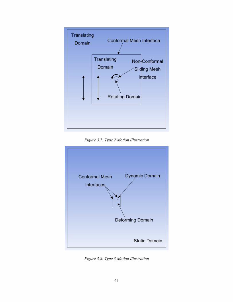
41

Figure 3.7: Type 2 Motion Illustration

Figure 3.8: Type 3 Motion Illustration

Translating

Domain Conformal Mesh Interface

Non-Conformal

Sliding Mesh

Interface

Rotating Domain

Translating

Domain

Dynamic Domain Conformal Mesh

Interfaces

Deforming Domain

Static Domain

42

Figure 3.9: Overview of Mesh Used for Type 3 Motion

Figure 3.10: Deforming Domain Mesh View for Type 3 Motion

43

Figure 3.11: Dynamic Domain Mesh View for Type 3 Motion

3.4.2 Results and Discussion

The results for the average CP are shown in Table 3.2 and the instantaneous CP over the last cycle

is shown in Figure 3.12. Type 3 predicts a slightly lower value in the translational and a slight

deviation is noticed at the normalized time of 0.07. These differences could be due to the fact that

the starting mesh was not identical to the type 1 and 2 meshes. Another reason for the possible

difference is that during the simulation, there is constant re-meshing occurring, so the final mesh

would be different that the one shown at the beginning of the simulation.

Table 3.2: Comparison of Results for Different Motion Types

Motion Type Average CP in

Last 3 Cycles

CP % Difference to

Type 1 Application

1 0.504 - Single Blade in 2D

2 0.506 0.4 Single Blade in 3D

3 0.499 1 Multi-Blade in 2D & 3D

44

Figure 3.12: Instantaneous CP versus Normalized Time of the 10th Cycle for Motion Types

Based on the CP, the results for the three motion types still came to be very close to each other.

The advantage of type 1 and 2 motions are shorter simulation time when compared to type 3 since

no re-meshing occurs during the simulation; however, both type 1 and type 2 are limited to only

having a single blade in the simulation. With type 3 motion, it is possible to have as many blades

as needed in the simulation. However, the simulation time is longer and due to the fact that the

mesh deforms and re-meshes throughout the simulation, additional interpolation errors are

introduced. For the remainder of the 2D investigation, type 1 is used, where possible, for a single

blade analysis as it is among the simplest and avoids any potential problems or errors from having

the domain boundaries move. Type 2 will be used for 3D simulations to maintain the speed of the

calculation but more importantly is to avoid certain complication with Fluent in 3D when using

Type 1 motion. Type 3 will only be used for the parametric study of a multi-blade turbine.

3.5 Mesh Convergence Study using SST k-ω Model with 𝒚+~ 1

Previously, a mesh of 135,000 elements was used for the initial testing of the turbine concept. This

mesh was based on the finest mesh of other’s simulations with the same Reynolds number of

500,000 [21]. However, at this point, it was necessary to perform a grid convergence study to

determine the necessity of using either a coarser more efficient mesh or perhaps a more refined

mesh to more accurately estimate the D-VAWT performance. In this section, a mesh independency

study is performed to determine the most efficient mesh. Since it is necessary to perform 3D

-0.75

-0.5

-0.25

0

0.25

0.5

0.75

1

1.25

1.5

1.75

0 0.1 0.2 0.3 0.4 0.5 0.6 0.7 0.8 0.9 1

CP

Normalized Time (t/T)

Type 1

Type 2

Type 3

45

simulations, having the coarsest mesh possible in 2D will significantly reduce the element count

in 3D and improve computational time. For this study, the SST k-ω turbulence model with low

Reynolds number correction is used with a 𝑦+ ~ 1 as it known to have higher accuracy, especially

since the entire boundary layer is resolved instead of being approximated with a wall function. In

section 3.6, a turbulence model comparison is done with the selected mesh from this study to

determine the effect of turbulence model choice on the results.

3.5.1 Meshes

Based on the previous investigation, type 1 motion is used with the domain sizes of 150C, 75C

and 2D for the static, translating and rotating domains, respectively. Three meshes are employed

for this study. An initial mesh of 45,000 elements, named Mesh 1, is used for the coarsest case.

Instead of doing two levels of mesh refinement with a factor of 1.35, as recommend by Roache

[62] based on the Grid Convergence Index (GCI) method developed from the theory of the

generalized Richardson Extrapolation, the intermediate mesh was skipped. The finest mesh is

refined with a factor of 2 or ~1.42. However, two meshes are tested (Mesh 2 and 3) at this

refinement factor of 2 relative to the starting mesh (Mesh 1), with the difference being Mesh 2

excludes the refinement of the boundary layer elements. This approach makes it possible to

determine the refinement effect from the mesh outside the boundary layer and then the effect of

the boundary layer refinement separately. The mesh details are summarized in Table 3.3 and the

meshes used can be seen in Figure 3.13 to Figure 3.18. The elements inside the rotating domain

are now quadrilateral elements instead of triangular for two reasons. The first and most important

reason is that in case the boundary layer flow does go beyond the boundary layer elements, quad

elements are much better at capturing it. Also, for the same sized elements, quad elements fill the

mesh with a smaller number of total elements when compared to triangular ones. One interesting

technique used for the generation of the inflation layer can be seen in the trailing edge view of

Figure 3.15, where one can see that the trailing edge is rounded and not included in the inflation

layer. Typically, the inflation layer encapsulates the entire airfoil profile, however, this technique

allows for much higher overall element quality for the boundary layer elements as it avoids

stretching the boundary layer elements to have them meet at the tailing edge.

46

Table 3.3: Details of Each Mesh Used for Mesh Study

Mesh 1 Mesh 2 Mesh 3

Element Size in Rotating Domain 0.02C 0.01C 0.01C

Element Size in Refinement Region 0.2C 0.1C 0.1C

Number of Nodes on Airfoil 500 500 1000

𝒚+ ~ 1 ~ 1 ~ 1

First Layer Height in Boundary Layer 7.5×10-5 C 7.5×10-5 C 7.5×10-5 C

Number of Boundary Layer Elements 50 50 85

Boundary Layer Growth Rate 1.1 1.1 1.05

Total Number of Elements 45K 72K 133K

Figure 3.13: Rotating Domain Mesh View for Mesh 1

47

Figure 3.14: Refinement Region Mesh Around Blade for Mesh 1

Figure 3.15: Boundary Layer Views for Mesh 1 at Leading Edge (Top), Mid-Chord (Middle), and

Trailing Edge (Bottom)

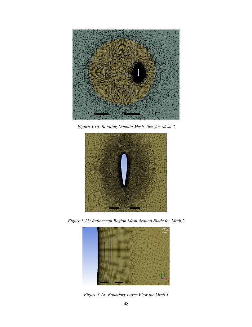
48

Figure 3.16: Rotating Domain Mesh View for Mesh 2

Figure 3.17: Refinement Region Mesh Around Blade for Mesh 2

Figure 3.18: Boundary Layer View for Mesh 3

49

3.5.2 Results and Discussion

All simulations performed in 2D are now run for 15 cycles. Even though at the 10th cycle the cycle

to cycle convergence was only less than 1%, the CP was still dropping. However, after the 15th

cycle, the CP only changed by about 0.01%, thus reaching satisfactory convergence. The

convergence of the average CP per cycle for Mesh 1 can be seen in Figure 3.19. The same trend is

noticed for all the other cases. Therefore for 2D simulations, 15 cycles is sufficient and the last

three cycles are averaged to be used as point of comparison.

Figure 3.19: Average Cycle CP Convergence Plot for Mesh 1

Table 3.4 shows the results from the mesh convergence study, where the percent difference from

the original mesh (Mesh 1) is presented. Even comparing the coarsest mesh (Mesh 1) with the

finest (Mesh 3) with the finer time step, the difference between them is less than 1%. In Figure

3.20, it can be seen that the only small differences that do appear are all near peak power positions,

but the same exact behavior is noticed for all of them. Based on this result, the coarsest mesh and

time step size are determined to be adequate for further investigation in 2D as well as 3D since the

cheapest mesh possible is needed for 3D purposes to reduce its high computational cost.

Table 3.4: Mesh and Time Convergence Study Results

Mesh Time step per

period Average CP

CP % Difference

to Mesh 1

1 1136 0.577 -

2 1136 0.580 0.50

3 1136 0.581 0.69

3 2274 0.582 0.86

0.890

0.774

0.7020.665

0.639 0.621 0.611 0.600 0.595 0.590 0.584 0.583 0.579 0.577 0.577

0.30

0.40

0.50

0.60

0.70

0.80

0.90

1.00

0 2 4 6 8 10 12 14 16

CP

Cycle

50

Figure 3.20: Instantaneous CP versus Normalized Time at 15th Cycle for Mesh and Time Convergence

Study Cases

3.6 Turbulence Model Study

In this section, the D-VAWT is simulated using different turbulence models to investigate the

accuracy of the results and justify the selection of the turbulence model. Three turbulence models

are considered in four cases: the one-equation SA Strain/Vorticity model with 𝑦+ ~ 1 and ~ 30,

the two-equation SST k-ω model with 𝑦+~ 1, and the four-equation transition SST model with

𝑦+~ 1. The fastest would be the SA Strain/Vorticity model 𝑦+~ 30 because it is a lower equation

model and the mesh needed for 𝑦+~ 30 is cheaper. The most expensive would be the transition

SST model since it is the highest equation model with a more refined mesh to achieve a 𝑦+~ 1.

The domain and mesh used in this study is the coarsest mesh (Mesh 1) with Δt = T/1136.

The results for the average CP for the different cases are shown in Table 3.5 and Figure 3.21. The

Transition SST model predicts the highest CP value, while the SA Strain/Vorticity for 𝑦+~ 30

predicts the lowest. The biggest difference is noticed between the cases using the mesh of 𝑦+~ 1

and 𝑦+~ 30. Though the trends shown in Figure 3.21 for all cases are similar, the SA

Strain/Vorticity with 𝑦+~ 30 under predicts the upstream translational region and the following

rotating region or at the normalized times between 0.22 and 0.72. It can be seen that the SA

-1

-0.5

0

0.5

1

1.5

2

0 0.1 0.2 0.3 0.4 0.5 0.6 0.7 0.8 0.9 1

CP

Normalized Time (t/T)

Mesh 1 Mesh 2 Mesh 3 Mesh 3 & Finer Time Step

51

Strain/Vorticity model at 𝑦+~ 30 consistently under predicts the CP value in that region, while for

the other models at 𝑦+~ 1 show better consistency in value throughout the cycle. The results

obtained here are also supported by [31], in which they showed at high TSR, the choice of

turbulence model with the same 𝑦+ has little effect on the results.

Table 3.5: Results for the Turbulence Model Study Using Mesh 1 at TSR =4.5

Turbulence Model 𝒚+ Average CP CP % Difference

to Case 1

SST k-ω 1 0.577 -

Transition SST 1 0.580 0.45

SA Strain 1 0.553 4.32

SA Strain 30 0.491 17.50

Figure 3.21: Instantaneous CP Plots of the 15th cycle for the Turbulence Model Study Using Mesh 1 at

TSR=4.5

-1

-0.5

0

0.5

1

1.5

2

0 0.1 0.2 0.3 0.4 0.5 0.6 0.7 0.8 0.9 1

CP

Normalized Time (t/T)

SST kw (y+1) Transition SST (y+1) SA Strain (y+1) SA Strain (y+ 30)

52

3.7 Airfoil Validation with Experimental Results

Using the presented methodology, an experimental case is simulated and the results are compared

with their respective experimental values. The case is that of a 2D simulation of a static airfoil.

This case was specifically chosen as it closely matched the flow regime of the D-VAWT while no

data was available for a Darrieus type turbine that even remotely resembled the D-VAWT’s flow

conditions and blade profile (NACA 0018).

Using the same methodology to generate the mesh, a NACA 0018 airfoil is simulated with an

identical numerical setup as the D-VAWT. The only difference from the D-VAWT case is the inlet

boundary condition values for the turbulent intensity, which were matched with the experimental

setup to ensure a proper comparison. The Reynolds number is 500,000, which is in the same range

as what the D-VAWT's blade experiences in the upstream translational region. The results are

validated with the experimental case performed by Timmer [63].

The purpose of these simulations is to validate the choice of turbulence model and accuracy of the

CFD setup with existing experimental results. The same four cases from the turbulence model

study are repeated here, which are the SA Strain/Vorticity model using 𝑦+~ 30 and 𝑦+~ 1, the SST

k-ω and transition SST models with 𝑦+~ 1.

3.7.1 Domain and Mesh

Figure 3.22 shows the overview of the domain and mesh used to replicate the experimental case.

The domain is a C-mesh type, which is commonly used for the simulation of static airfoils. Figure

3.23 shows a close view of the mesh near the blade for the cases of 𝑦+~ 30 and 𝑦+~ 1. The meshes

were generated with the same element sizes as for the case of the D-VAWT.

53

(a) (b)

Figure 3.22: Overview of (a) Domain (b) Mesh, for the Experimental Case Simulation

(a) (b)

Figure 3.23: Mesh Near Blade for (a) 𝑦+~ 30 (b) 𝑦+~ 1

3.7.2 Results and Discussion

Figure 3.24 to Figure 3.27 show the results for the Coefficient of Lift (CL) and Coefficient of Drag

(CD) for all simulations cases as well as the experimental values. Figure 3.24 shows that the

transition SST model predicts the most accurate results as it captures the experimental curve the

closest. The SST k-ω model is the second most accurate model tested, with the advantage of being

computational cheaper than the Transition SST. The SA Strain/Vorticity model with 𝑦+ ~ 1 over

predicts drag, as seen in Figure 3.25, while the SA Strain/Vorticity model with 𝑦+ ~ 30 greatly

over predicts drag and shows premature stall behavior that is not seen with any of the other models

at 𝑦+ ~ 1. This further explains the under prediction of the SA Strain/Vorticity model with 𝑦+ ~

30 in the results of Figure 3.21, where the blade experienced higher drag and lower lift than it

should have. This finding further supports the results of the turbulence model study.

50C

75C

54

Figure 3.24: Coefficient of Lift vs Angle of Attack

Figure 3.25: Coefficient of Drag vs Angle of Attack

0

0.2

0.4

0.6

0.8

1

1.2

1.4

3 5 7 9 11 13 15 17

CL

Angle of Attack (deg)

Exp

SST kw (y+1)

Transition SST (y+1)

SA Strain (y+1)

SA Strain (y+30)

0

0.01

0.02

0.03

0.04

0.05

0.06

0.07

0.08

0.09

0.1

3 5 7 9 11 13 15 17

CD

Angle of Attack (deg)

Exp

SST kw (y+1)

Transition SST (y+1)

SA Strain (y+1)

SA Strain (y+30)

[63]

[63]

55

Figure 3.26: Ratio of Coefficient of Lift to Coefficient of Drag vs Angle of Attack

Figure 3.27: Coefficient of Lift vs Coefficient of Drag

0

10

20

30

40

50

60

70

3 5 7 9 11 13 15 17

CL/

CD

Angle of Attack (deg)

Exp

SST kw (y+1)

Transition SST (y+1)

SA Strain (y+1)

SA Strain (y+30)

0

0.2

0.4

0.6

0.8

1

1.2

1.4

0 0.02 0.04 0.06 0.08 0.1

CL

CD

Exp

SST kw (y+1)

Transition SST (y+1)

SA Strain (y+1)

SA Strain (y+30)

[63]

[63]

56

Table 3.6 shows the percent error for all data points simulated for all turbulence models with the

values obtained from the experimental data. The interesting part to note is the average error for the

ratio of CL to CD for the range of angle of attacks that the D-VAWT experiences (from 0o to 12.5o)

at TSR = 4.5 for the cases of SA Strain/Vorticity model using a 𝑦+~ 30 and 𝑦+~ 1, the SST k-ω

and transition SST models with a 𝑦+~ 1 are 44.9%, 18.6%, 2% and 0.6%, respectively. These

values confirm that the transition SST model provides the most accurate solution, closely followed

by the SST k-ω model, while the SA Strain/Vorticity model provides the least accurate results for

both 𝑦+ cases. The ratio of CL to CD is directly related to the predicted output power of the turbine.

Seeing that the SA Strain/Vorticity with 𝑦+~ 30 consistently under predicts that said ratio, this

explains the under prediction in power for the case of the D-VAWT.

Table 3.6: Percent Error for Airfoil Case Study (Positive is Over Prediction and Negative is Under

Prediction)

% Error with Experimental Results

SST kw (𝒚+~ 1) Transition SST

(𝒚+~1) SA Strain (𝒚+~ 1) SA Strain (𝒚+~ 30)

Angle of

Attack CD CL CL/CD CD CL CL/CD CD CL CL/CD CD CL CL/CD

3 7.68 3.85 -3.55 -3.96 -18.9 -15.5 49.91 3.44 -31.00 75.78 -2.83 -44.72

6 6.12 2.93 -3.01 7.84 3.58 -3.95 42.21 2.34 -28.04 74.24 -3.55 -44.65

9 -6.06 -5.93 0.13 -0.90 6.11 7.07 21.84 -6.92 -23.61 60.98 -13.51 -46.27

10 -2.49 0.28 2.84 3.11 8.27 5.01 22.35 -0.24 -18.46 67.42 -8.22 -45.18

11 -1.15 4.30 5.51 4.08 6.41 2.24 18.84 4.65 -11.94 69.80 -5.28 -44.22

12.5 -2.82 7.50 10.62 4.98 6.34 1.29 8.15 9.86 1.57 70.29 -4.92 -44.17

13 -3.05 8.42 11.83 7.24 6.08 -1.08 4.67 11.67 6.69 73.08 -5.78 -45.57

14 -8.63 9.49 19.82 4.24 5.74 1.44 -8.31 15.21 25.66 75.09 -10.75 -49.03

15 -12.0 8.07 22.83 1.93 3.57 1.61 -20.17 17.80 47.57 88.41 -22.33 -58.78

Avg. -2.49 4.32 7.45 3.17 3.02 -0.21 15.50 6.42 -3.51 72.79 -8.57 -46.95

Avg. (up

to 12.5o) 0.21 2.15 2.09 2.53 1.97 -0.65 27.22 2.19 -18.58 69.75 -6.38 -44.87

3.8 Summary and Conclusions

The validation for the D-VAWT included the investigation of the domain size, motion prescription

methods, mesh and time convergence, and turbulence model study. The setup was also validated

with an airfoil case study with experimental data. The validation allowed us to find the smallest

domain, mesh and time step needed to make this setup the most conservative and cheapest while

still retaining satisfactory accuracy. Having the cheapest possible setup will greatly help in

reducing the cost of 3D simulations as they tend to be quite expensive.

57

The theoretical calculation of the CP, shown in section 2.6, for the upstream translational region

predicted a value of 1.41. This calculation was done for an airfoil with an angle of attack of 12.5o

and a blade Reynolds number of 500,000, which are the conditions the D-VAWT blade during the

translational section. The average value of CP in the upstream translational region using the SST

k-ω model is 1.38. Comparing the theoretical and predicted CFD values, there is only a difference

of about 2%, which further supports the analysis and the selected methodology.

Based on the turbulence model study and the validation with experimental results, the SST k-ω

model at 𝑦+~ 1 and the SA Strain/Vorticity model at 𝑦+~ 30 provide an upper and lower bound

estimate for the CP, where the lower bound will represent a more conservative estimate for the D-

VAWT’s performance. The upper and lower bounds can be clearly seen in Figure 3.26. The reason

the SST k-ω model was chosen over the other two models at 𝑦+~ 1 is that it is faster than the

Transition SST model and it is more accurate at resolving the boundary layer flow in the near-wall

region than the SA Strain/Vorticity model. The value predicted from the SST k-ω model is

expected to represent actuality more closely than from the lower bound estimate because it is a

higher equation model capable of accurately resolving the flow in the near-wall region. For airfoil

and turbine simulations where there is no shedding of vortices, accurately capturing the boundary

layer flow is of the utmost importance, which is exactly what the SST k-ω model is good at

resolving.

58

CHAPTER 4: 3D INVESTIGATION

In this chapter, 3D simulation of the D-VAWT at TSR = 4.5 with the same geometrical

parameters as presented earlier will be performed based on the methodology developed in the

previous chapter. The Aspect Ratio (AR) of 5 and 15 will be investigated using the SA Strain (𝑦+~

30) and SST k-ω (𝑦+~ 1) turbulence models to provide us with an upper and lower bound estimate

of the CP.

4.1 Domain

The domain used for the simulation with AR = 5 is shown in Figure 4.1. Further details are included

in Table 4.1 for both domains of AR = 5 and 15. It should be noted that only half of the blade is

simulated by making use of a symmetry plane boundary condition. This essentially allows the

domain to be cut by half, which significantly reduces the computational cost.

Type 2 motion is used for all 3D simulations since Fluent encountered many problems with the

deforming mesh of type 1 motion. Based on the comparison of motion types, the results should be

identical for both motions. The coordinate system is shown in Figure 4.1, where the incoming wind

is coming in the positive X-direction.

Figure 4.1: 3D Domain for D-VAWT with AR=5

150C 30C 150C

59

Table 4.1: 3D Domain Characteristics

3D Domain Characteristics

Aspect Ratio = 5 Aspect Ratio =15

Outer Domain Size 150C × 150C × 30C 150C × 150C × 45C

Simulated Blade Height, h/2 2.5C 7.5C

Rotating Domain Diameter 2D 2D

Rotating Domain Depth 3.25C 8.25C

4.2 Mesh

Two turbulence models are tested, the SA Strain/Vorticity and SST k-ω, with different 𝑦+

strategies for each. There are a total of four cases performed, comprising of two aspect ratios with

two turbulence models. The details of the mesh used are shown Table 4.2, which are based on the

2D mesh study. The mesh for the AR = 5 with the SA Strain/Vorticity model is shown in Figure

4.2 to Figure 4.5, while the one used for AR = 5 with the SST k-ω model is shown in Figure 4.6

to Figure 4.8. The meshes used for each turbulence model are nearly identical; the only difference

is the number of elements in the span wise direction for the different aspect ratios used. Elements

across the rotating interface are matched in size to reduce interpolation errors across the interface.

The elements in the refinement region around the blade are hexahedron elements formed from

quadrilateral elements that have been swept in the span-wise direction. It should be noted that the

elements swept have a bias towards the blade tip, meaning the elements near the blade tip are

smaller than the ones near the blade center (at the symmetry plane). The purpose of the bias is to

better capture the flow and pressure drop near the blade end from the tip vortex. All the elements

outside of the refinement regions are tetrahedrons.

60

Table 4.2: 3D Meshes Details

Case

Aspect Ratio = 5 Aspect Ratio =15

SA Strain SST k-ω SA Strain SST k-ω

Element size in rotating domain 0.2C 0.2C 0.2C 0.2C

Element size in refinement region 0.02C 0.02C 0.02C 0.02C

Number of nodes on airfoil 250 500 250 500

Number of span wise elements 80 80 200 200

𝒚+ ~ 30 ~ 1 ~ 30 ~ 1

First layer height in boundary layer 2.5×10-3 C 7.5×10-5 C 2.5×10-3 C 7.5×10-5 C

Number of boundary layer elements 15 50 15 50

Boundary layer growth rate 1.1 1.1 1.1 1.1

Total number of elements 2.9 Million 4 Million 7.5 Million 10 Million

Figure 4.2: Rotating Domain Mesh at Symmetry Plane for AR=5 and 𝑦+~ 30

61

Figure 4.3: Refinement Region Mesh at Symmetry Plane for AR=5 and 𝑦+~ 30

Figure 4.4: Boundary Layer Mesh View at Symmetry Plane for AR=5 and 𝑦+~ 30

Figure 4.5: Cross Section of Mesh Around the Blade AR=5 and 𝑦+~ 30

62

Figure 4.6: Refinement Region Mesh at Symmetry Plane for AR=5 and 𝑦+~ 1

Figure 4.7: Boundary Layer Mesh View at Symmetry Plane for AR=5 and 𝑦+~ 1

Figure 4.8: Cross Section of Mesh Around the Blade for AR=5 and 𝑦+~ 1

63

4.3 Numerical Setup

The SIMPLE algorithm is selected for the pressure-velocity coupling. For the spatial

discretization, second order schemes are used for the pressure, momentum and turbulent viscosity

calculation. First order implicit is still used for the transient formulation due to the use of the

dynamic mesh capabilities. All simulations are performed with an absolute convergence criterion

of 10-3 for the continuity, velocity components and all turbulent properties. The time step size is

Δt = 0.5585ms or about one thousandth of a period (T/1136). The SA Strain/Vorticity based

production model and the SST k-ω model with low Reynolds number correction are used for

turbulence modelling.

The boundary conditions are shown in Figure 4.9, where constant and uniform velocity inlets are

defined everywhere, except for the bottom plane which has a symmetry condition and the right

most boundary is defined as a pressure outlet. The velocity of incoming wind is 4 m/s with a

turbulent intensity of 1% and a turbulent viscosity ratio of 𝜈𝑡

𝜈= 5. The turbulent intensity is

reduced from 5% to 1% from the 2D to 3D simulations to speed up the convergence of the

simulation. This change would have marginal effect on the results as both turbulence intensities

were tested and compared in 2D. As for the blade boundary condition, a no-slip condition is

applied.

Figure 4.9: Boundary Conditions for 3D Domains

4.4 Results and Discussion

All 3D simulations of the D-VAWT at TSR = 4.5 were run for 10 and 12 cycles for the aspect ratio

of 5 and for 15, respectively. The CP cycle convergence can be seen in Figure 4.10, where it can

be noticed that the simulations with AR = 5 converge faster than the ones with AR = 15. The cycle

64

to cycle convergence criterion used for all 3D simulations is 0.2%, since matching that of 2D’s of

0.01% was difficult to reach in 3D. Table 4.3 presents the summary of the averaged CP in the last

3 cycles and the ratio of 3D to 2D CP values for each case respectively. It can be seen that for the

AR of 5, only about 40-44% of the power in 2D is captured, while for an AR of 15, this increases

to about 70%. The 3D to 2D ratio value for the AR =15 case is also supported by [31], where a

ratio of 69% is obtained for the same AR. It is well known that as the AR of airfoil blades is

increased, the 3D performance approaches that of 2D. For a short AR, the 3D losses, especially

because of the formation of a wing tip vortex, dominate and a larger portion of the blade sees a

large decrease in performance. The formation of the wing tip vortex leads to a decrease in

performance as a result of the pressure drop on the blade surface when approaching the blade tip.

The wing tip vortex allows the flow to “leak” over the blade tip and reduces the built up pressure

from the airfoil profile, which in turn reduces the lift of the blade portion affected by it.

Figure 4.10: Average CP per Cycle Convergence for 3D Simulations

Table 4.3: CP Results Summary for 3D Simulations

Aspect Ratio Turbulence Model Average CP 3D/2D % Ratio

5 SA Strain (𝑦+~ 30) 0.198 40.37

SST k-ω (𝑦+~ 1) 0.253 43.73

15 SA Strain (𝑦+~ 30) 0.338 68.86

SST k-ω (𝑦+~ 1) 0.404 70.03

0.198

0.337

0.252

0.402

0.000

0.100

0.200

0.300

0.400

0.500

0.600

0.700

0.800

0 2 4 6 8 10 12 14

CP

Cycle

SA Strain (y+ 30), AR =5

SA Strain (y+ 30), AR = 15

SST kw (y+1), AR = 5

SST kw (y+1), AR = 15

65

The instantaneous CP curves are shown in Figure 4.11 for all 3D cases. For the same AR, there is

a gap in performance between the SA Strain/Vorticity model and SST k-ω model, where the SA

Strain/Vorticity model with 𝑦+~ 30 still under predicts the CP values, most noticeably in the

upstream translational region and the following rotational region. The CP trend between the blade

of AR of 5 and 15 are similar throughout most of the cycle, except for the fact that the blade of

AR of 15 produces more power as expected. An interesting behavior between the two is noticed

in the downstream portion of the blade path, especially in the translational region. For the AR of

15, CP behavior is very similar to that of the 2D one, but for the AR of 5, looking at the normalized

time from 0.72, the CP is initially slightly higher than for the AR of 15, but after t/T=0.88, a dip in

power occurs that is not seen in either the 2D or 3D with AR=15 cases.

Figure 4.11: Instantaneous CP Plots of the Last Cycle for 3D Simulations

In Figure 4.12, the normalized velocity deficit ( U∞−U

U∞) is shown at a cross sectional plane that is

half a chord away from the symmetry plane as it is preferable not to visualize the flow on the

symmetry plane. The normalized velocity deficit shows how much velocity is either reduced from

losses or extracted by the turbine. Figure 4.12 (a) and (b) are for the SA Strain/Vorticity model of

AR = 5 and 15, respectively. It should be noted that the blade tip effect is stronger for the case of

AR = 5 at this plane because this plane is only two chords away from the tip while for the AR =

15, it is 7 chords away. A plane that is two chords away from the blade tip was visualized for the

-0.75

-0.5

-0.25

0

0.25

0.5

0.75

1

1.25

1.5

0 0.1 0.2 0.3 0.4 0.5 0.6 0.7 0.8 0.9 1

CP

Normalized Time (t/T)

3D SA Strain (y+ 30), AR =5 3D SA Strain (y + 30), AR = 15

3D SST kw (y+1), AR = 5 3D SST kw (y+1), AR = 15

66

case of AR = 15, it was then noticed that the behavior of the flow highly resembled that of the AR

= 5 shown here. This means that at a distance of two chords from the blade tip for either AR = 5

or 15 cases, the performance of the blade is highly affected and reduced by the presence of the

wing tip vortex, while at 7 chords away for AR = 15, this effect dissipates and the performance

approaches that of 2D. To better grasp the effect of AR on the blade performance, Figure 4.13

shows the static pressure contour on the blade surface during the upstream translational region for

the SST k-ω model for both AR 5 and 15. One can see the pressure drop starting from around one

chord’s length from the blade tip and because about the same length of the blade is affected for

both ARs, it means that the blade with AR = 5 has a larger portion affected.

As shown in Figure 4.12, after the upstream pass of the blade, about 35-40% of the free stream

velocity is extracted or lost, while after the downstream pass, the free stream velocity drops to 75-

80% of its initial value. This means that with a single turbine, it is possible to extract about 75%

of the incoming wind’s energy from the two passes of the blade in the translational region. This

can also be supported from the CP values seen in those regions. However, with such a strong

velocity deficit, the wake of this turbine will be very strong and will take some time to recover and

return to its original free stream velocity. This means that if another turbine were to be placed

downstream of it, it would have to be significantly far away from the first.

Another detail to note from Figure 4.12 is that for the same AR in Figure 4.12 (a) and (c), the flow

for the SA Strain/Vorticity and the SST k-ω models have similar wake structure, but for the SST

k-ω model, the velocity deficit in the wake is higher, which can be explained by the higher power

extraction seen in the CP Curve. This can also be seen again in Figure 4.12 (b) and (d). The

difference between the models can be seen in the size of the boundary layer in Figure 4.14, where

the turbulent viscosity ratio ( 𝜈𝑡

𝜈) is shown at the same cross sectional plane as before, but at the

normalized time t/T = 0.33, which is approximately midway in the translational region. In Figure

4.14, the AR does not seem to affect the size of the boundary layer, but the choice of 𝑦+ between

the two models does indeed affect it, resulting in a boundary layer for the 𝑦+~ 30 to be almost

twice as thick as the one for 𝑦+~ 1. The recirculation zone on the suction side to the airfoil (right

side of blades in Figure 4.14) is also much larger for the cases with 𝑦+~ 30, leading to lower lift

and higher drag as seen before in the results of the experimental validation case of a static airfoil,

which explains the lower extracted power in this region.

67

(a) (b)

(c) (d)

Figure 4.12: Normalized Velocity Deficit ( 𝑈∞−𝑈

𝑈∞) Plots on a Plane of Half a Chord Away in the Span-

Wise Direction from the Symmetry Plane at t/T=0.68 for Cases (a) SA Strain/Vorticity (𝑦+~ 30) with AR

=5, (b) SA Strain/Vorticity (𝑦+~ 30) with AR =15, (c) SST k-ω (𝑦+~ 1) with AR =5, and (d) SST k-ω

(𝑦+~ 1) with AR =15

Normalized Velocity Deficit, 𝐔∞−𝐔

𝐔∞

0.00 1.00 0.50 0.25 0.75

68

(a)

(b)

Figure 4.13: Static Pressure Contour on Half of the Blade Surface for SST k-ω (𝑦+~ 1) Model at

t/T=0.33 for (a) AR = 15 (b) AR = 5

Figure 4.14: Turbulent Viscosity Ratio ( 𝜈𝑡

𝜈) Plots on a Plane of Half a Chord Away in the Span-Wise

Direction from the Symmetry Plane at t/T=0.33 for Cases (a) SA Strain/Vorticity (𝑦+~ 30) with AR =5,

(b) SA Strain/Vorticity (𝑦+~ 30) with AR =15 and (c) SST k-ω (𝑦+~ 1) with AR =5, and (d) SST k-ω (𝑦+~

1) with AR =15

Static Pressure [Pa]

-500 50 -225 -362.5 -87.5

(a) (d) (c) (b)

Turbulent

Viscosity Ratio, 𝛎𝐭

𝛎

0

30

15

7.5

22.5

69

4.5 Comparison of 2D and 3D Results

Figure 4.15 compares the 2D and 3D results for all cases simulated with the SST k-ω models. It

can be seen that as the AR increases, the power curve approaches the 2D results in value and

behavior, which is the expected behavior since 2D is considered to be a blade that is infinitely

long. This further supports the analysis and the methodology transition from 2D to 3D.

Figure 4.15: Comparing Instantaneous CP for 2D and 3D with AR =5 and 15 Using the SST k-ω Model

(𝑦+~ 1)

The following work will continue the investigation of the D-VAWT to further understand the flow

and turbine behavior for different geometrical parameters and operating conditions. The next

simulations of the D-VAWT will be performed in 2D only as the trends and behaviors predicted

will still be valid for future designs, while the results can be obtained in a matter of days instead

of months. To put in perspective, the longest 3D simulation was performed on a cluster of 24 cores

with 2.67 GHz processing frequency, which took over eight weeks to complete, while 2D

simulations were performed on 12 cores and finished in a matter of hours instead.

-0.75

-0.5

-0.25

0

0.25

0.5

0.75

1

1.25

1.5

1.75

2

0 0.1 0.2 0.3 0.4 0.5 0.6 0.7 0.8 0.9 1

CP

Normalized Time (t/T)

AR = 5 AR = 15 2D

70

4.6 Discussion of D-VAWT Performance

Considering the D-VAWT performance for an AR of 15, the lower and upper bound of the CP are

0.34 and 0.404, respectively. The actual value would be closer to the upper bound as the

simulations with 𝑦+~ 30 (the lower bound) do not capture the boundary layer flow as accurately

as the ones with 𝑦+~ 1. This finding is supported from the results of the turbulence model and the

experimental airfoil case study. Although 3D simulations are much more accurate than 2D

simulations, they will still have some level of over prediction of the turbine performance. One

should remember that this study is based on a numerical approach, which represents an idealized

system where a number of losses are not taken into account. The unconsidered losses include the

generator and mechanical losses as well as aerodynamic losses from the lack of simulating the

structural components of the turbine. Nonetheless, the predicted CP values for a straight blade

Darrieus type turbine is high, considering this range of CP is usually seen for the more

aerodynamically efficient rotor Darrieus turbines and HAWTs. However, the D-VAWT is still far

from being fully optimized. A simple improvement would be to use endplates for the blade, which

would reduce the 3D aerodynamic losses and the CP would further approach the 2D approximation.

Based on the results of this study, the D-VAWT concept of extending the region of maximum

power production did improve the overall turbine performance. Most performance improvement

studies on VAWTS are conducted on optimizing blade profile or other geometric parameters,

while the D-VAWT concept is among the few studies that investigated a new and unconventional

blade path for a turbine. The following chapter continues with the parametric study to further

understand and optimize the D-VAWT.

As mentioned earlier, the CP for the D-VAWT is high; one should note that it is even more

impressive that it is this high for small scale applications. Typically, this range of CP is difficult to

achieve on small scale, even for the HAWTs as they too lose a large portion of their efficiency for

small scale application. However, this high performance turbine does come with some drawbacks.

The D-VAWT requires the wind to be normal to its longitudinal side for optimal performance,

meaning if the wind changes direction, the performance of the turbine will deteriorate depending

on how deviated the incoming flow angle is. This is a new weakness that typical other VAWTs do

not suffer from. It should be noted that there are solutions to account for different incoming wind

directions. The simplest would be to design a shroud to align the flow and provide the D-VAWT

with a wider range of operating of incident wind angles. The more complex solution would be a

71

mechanical one, where one of the two axes’ will be allowed pivot in order to always have the

turbine longitudinal side to be normal to the incoming wind. The other drawback for the D-VAWT

is the higher mechanism complexity compared to the typical VAWT, which are generally quite

simple from a mechanical point of view.

72

CHAPTER 5: 2D PARAMETRIC STUDY

Having completed the validation in 2D and obtained a more realistic performance from the

3D simulations, this chapter presents 2D simulations to further understand and optimize the D-

VAWT’s performance. Though the results in 2D will over predict the CP values, the trends

obtained in 2D will still be valid and can be incorporated into future 3D designs. The parametric

study will include the investigation of the sensitivity to change in wind direction, two bladed

turbine, AEF study, high lift airfoil, and blade mounting location. The goal of this chapter is not

to perform a detailed parametric study, but it is to serve as the first steps in understanding the D-

VAWT’s behavior to help guide future studies.

5.1 Introduction to Parametric Study

In this chapter, all simulations are performed using the SST k-ω (𝑦+~ 1) setup since it is capable

of capturing the boundary layer more accurately than the SA Strain/Vorticity model setup. For

each parameter investigated, a range of TSRs is performed to find the point of peak performance.

The goal is not to capture the entire CP curve (CP vs. TSR), but to find the effect on the location

and value of the peak CP. One should note that the CP curve should follow a quadratic curve. For

each range of TSRs performed, a quadratic curve will also be fitted from the data for comparison

and support of the analysis.

Eq. (5.1) provides the instantaneous angle of attack for different azimuthal angle and TSR values.

Figure 5.1 plots the change of angle of attack during the blade rotation of a VAWT for different

TSR values. One can see the drop of the maximum angle of attack as the TSR is increased. Below

a certain TSR, typically lower than TSR = 3, the blade could start to go through dynamic stall and

shedding of vortices will occur from flow separation. Since the D-VAWT operates at high TSRs,

there are almost no cases where the blade dynamically stalls.

𝛼 = tan−1 (

sin 𝜃

cos 𝜃 + 𝜆) (5.1)

73

Figure 5.1: Instantaneous Blade Angle of Attack for Darrieus Type VAWT vs Azimuthal Angle for

Different TSRs

5.2 TSR Study of Original Turbine

The first step of the parametric study is to find the CP curve for the original turbine to have a base

for comparison when changing the turbine parameters as well as find out at which TSR the turbine

has maximum performance. This turbine is still simulated with a single blade at AEF = 4.

The results of the simulation are shown in Figure 5.2, Figure 5.3, and Figure 5.4. It should be noted

that the case for the TSR = 4.5 is repeated again here and one can see the CP value changed from

0.577 to 0.587. The marginal difference is due to some corrections made in the UDF code, which

controls the motion switching criterion between translating to rotating motions. The UDF was only

modified now as to have consistent methodology between chapter 3 and 4 and allow for direct

comparison between them.

Figure 5.2 shows the cycle to cycle convergence of CP, where it can be seen that the higher the

TSR, the more cycles are required to reach the same convergence as the lower TSR cases. This

trend is noticed for all cases simulated in this chapter, where the high TSR cases required a higher

number of cycles for convergence. From TSR 3.5 to 5, there is less than 6% drop in performance

from the peak point, which makes this curve quite “flat” (insensitive to change in TSR) compared

to other wind turbines as seen in the CP curve shown in Figure 5.3. In other words, the insensitivity

-50

-40

-30

-20

-10

0

10

20

30

40

50

0 30 60 90 120 150 180 210 240 270 300 330 360

An

gle

of

Att

ack

(deg

)

Azimuthal Angle (deg)

TSR = 1.5

TSR = 2

TSR = 2.5

TSR = 3

TSR = 4

TSR = 5

TSR = 6

74

to the TSR can also mean that the performance is insensitive to the change in incoming wind

speeds if the turbine rotational speed was kept constant. Also from Figure 5.3, the graph confirms

that the peak CP is at TSR = 4.5, thus supporting the choice of TSR for the 3D analysis. One can

also see the points closely follow the quadratic curve fitted over the points, which also support the

methodology and analysis of this turbine.

Figure 5.2: Average Power Coefficient Convergence per Cycle for Different TSR values for AEF=4

Figure 5.3: Average CP per Cycle vs TSR for AEF= 4 with Quadratic Curve Fitting

0.40

0.50

0.60

0.70

0.80

0.90

1.00

1.10

1.20

0 5 10 15 20 25

CP

Cycle

TSR = 3.5

TSR = 4

TSR = 4.5

TSR = 5

TSR = 5.5

0.5540.583 0.587

0.555

0.507

0.00

0.10

0.20

0.30

0.40

0.50

0.60

0.70

3 3.5 4 4.5 5 5.5 6

CP

TSR

75

To further understand the behavior of the turbine at each TSR, Figure 5.4 shows the plots for the

instantaneous CP for all TSR cases. It can be seen that a higher TSR results in larger positive and

negative peaks throughout, except for the downstream translational region, where all TSR cases

converge to the same CP. One can also understand why most H-Darrieus turbines do not operate

at such high TSRs is because of the large negative CP peaks experienced in both rotating regions,

which is the entire H-Darrieus’ cycle of rotation.

One trend that can be extrapolated from the instantaneous CP curve is that by increasing the AEF

values, the higher TSRs will become more efficient as more time is spent where the highest

positive peaks are seen. This means the higher the AEF, the more the peak CP should move to

higher TSR values.

Figure 5.4: Instantaneous CP for Different TSR Values at AEF =4

-1.50

-1.00

-0.50

0.00

0.50

1.00

1.50

2.00

2.50

0.0 0.1 0.2 0.3 0.4 0.5 0.6 0.7 0.8 0.9 1.0

CP

Normalized Time (t/T)

TSR = 3.5

TSR = 4

TSR = 4.5

TSR = 5

TSR = 5.5

76

5.3 Incident Wind Angle

Since the D-VAWT is not circular in shape, its performance will change if the incoming wind is

not normal to its longitudinal side. This section attempts to determine the turbine sensitivity to the

incoming wind by simulating six cases and comparing their performances with the zero incident

angle presented in the previous section. The six incident wind angles are 𝜑 = ± 20°, ± 40°, ± 60°.

The convention for the incident wing angle is shown in Figure 5.5. One should remember that the

turbine swept area is reduced with increasing incident wind angle based on Eq. 2.38.

Figure 5.5: Incident Wind Angle Convention

The summary of the CP curves for all six cases and the original zero incident angle are shown in

Figure 5.6. As expected, the best performance is obtained with zero incident angle. All positive

incident angles perform better than their equivalent negative ones due to the negative angles

increasing the effective angle of attack on the blade in the upstream translational region, leading

to a reduced overall performance. At φ = + 20°, the CP curve highly resembles that of the zero

incident angle from a performance and trend point of view as well as even slightly surpassing its

performance at TSR = 5.5. This is an unexpected behavior and its explanation will be presented at

the end of this section. From the same figure, one can see that as the incident angle is increased,

both negative and positive angles, the performance worsens and the CP curve shifts to lower TSR

for its peak performance. Though a bit difficult to notice, the higher the incident angle, the more

sensitive the performance becomes to the change in TSR, which can be seen as the curve becoming

steeper compared to the flatter curve of zero incident angle. One can also see that all curves nicely

follow the quadratic curve fitting.

X

Y

U∞ at φ = 0°

φ +

φ -

77

Figure 5.6: Average CP for Different TSRs with Different Incoming Incident Wind Angles with Quadratic

Curve Fitting

Figure 5.7 and Table 5.1 summarize the peak CP performance of each case. From the graph, one

can notice the sharper and more linear drop in power from the negative incident angles. In Table

5.1, the peak CP for all cases are shown and compared as a percentage to the peak CP at zero

incident angle. At positive and negative incident angle of 20o, the turbine performs at 98.5% and

89.9% of the peak CP, respectively. This means for an AEF = 4, the turbine loses a maximum of

~10% power for a 40° incident angle range. This result is quite satisfactory as it means that the D-

VAWT still performs efficiently for a wide range of incident angles without critically losing its

original high efficiency.

Figure 5.8 to Figure 5.13 show the instantaneous CP curves for all performed TSRs for the incident

angles of - 20°, - 40°, - 60°, + 20°, + 40° and + 60°, respectively. From the figures, one can see as

the incident angle increase, the performance of both upstream and downstream translating regions

further deteriorates. For the cases of ± 60°, little to negative power is observed in the translating

regions. One can also notice that the rotating regions are also affected by the change in incident

angle, which was not expected as it was believed the performance in those sections should have

-0.20

-0.10

0.00

0.10

0.20

0.30

0.40

0.50

0.60

0.70

2.5 3 3.5 4 4.5 5 5.5 6

CP

TSR

Phi = - 60 deg

Phi = - 40 deg

Phi = - 20 deg

Phi = 0 deg (original)

Phi = + 20 deg

Phi = + 40 deg

Phi = + 60 deg

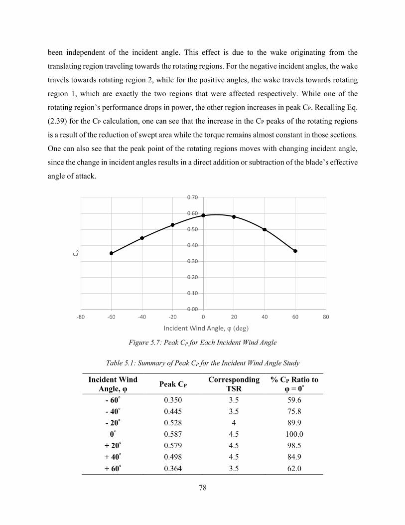
78

been independent of the incident angle. This effect is due to the wake originating from the

translating region traveling towards the rotating regions. For the negative incident angles, the wake

travels towards rotating region 2, while for the positive angles, the wake travels towards rotating

region 1, which are exactly the two regions that were affected respectively. While one of the

rotating region’s performance drops in power, the other region increases in peak CP. Recalling Eq.

(2.39) for the CP calculation, one can see that the increase in the CP peaks of the rotating regions

is a result of the reduction of swept area while the torque remains almost constant in those sections.

One can also see that the peak point of the rotating regions moves with changing incident angle,

since the change in incident angles results in a direct addition or subtraction of the blade’s effective

angle of attack.

Figure 5.7: Peak CP for Each Incident Wind Angle

Table 5.1: Summary of Peak CP for the Incident Wind Angle Study

Incident Wind

Angle, φ Peak CP

Corresponding

TSR

% CP Ratio to

φ = 0°

- 60° 0.350 3.5 59.6

- 40° 0.445 3.5 75.8

- 20° 0.528 4 89.9

0° 0.587 4.5 100.0

+ 20° 0.579 4.5 98.5

+ 40° 0.498 4.5 84.9

+ 60° 0.364 3.5 62.0

0.00

0.10

0.20

0.30

0.40

0.50

0.60

0.70

-80 -60 -40 -20 0 20 40 60 80

CP

Incident Wind Angle, φ (deg)

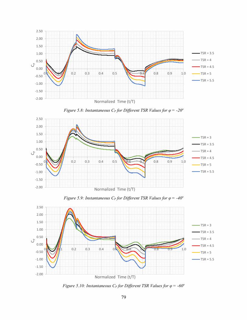
79

Figure 5.8: Instantaneous CP for Different TSR Values for φ = -20o

Figure 5.9: Instantaneous CP for Different TSR Values for φ = -40o

Figure 5.10: Instantaneous CP for Different TSR Values for φ = -60o

-2.00

-1.50

-1.00

-0.50

0.00

0.50

1.00

1.50

2.00

2.50

0.0 0.1 0.2 0.3 0.4 0.5 0.6 0.7 0.8 0.9 1.0

CP

Normalized Time (t/T)

TSR = 3.5

TSR = 4

TSR = 4.5

TSR = 5

TSR = 5.5

-2.00

-1.50

-1.00

-0.50

0.00

0.50

1.00

1.50

2.00

2.50

0.0 0.1 0.2 0.3 0.4 0.5 0.6 0.7 0.8 0.9 1.0

CP

Normalized Time (t/T)

TSR = 3

TSR = 3.5

TSR = 4

TSR = 4.5

TSR = 5

TSR = 5.5

-2.00

-1.50

-1.00

-0.50

0.00

0.50

1.00

1.50

2.00

2.50

0.0 0.1 0.2 0.3 0.4 0.5 0.6 0.7 0.8 0.9 1.0

CP

Normalized Time (t/T)

TSR = 3

TSR = 3.5

TSR = 4

TSR = 4.5

TSR = 5

TSR = 5.5

80

Figure 5.11: Instantaneous CP for Different TSR Values for φ = +20o

Figure 5.12: Instantaneous CP for Different TSR Values for φ = +40o

Figure 5.13: Instantaneous CP for Different TSR Values for φ = +60o

-2.00

-1.50

-1.00

-0.50

0.00

0.50

1.00

1.50

2.00

2.50

0.0 0.1 0.2 0.3 0.4 0.5 0.6 0.7 0.8 0.9 1.0

CP

Normalized Time (t/T)

TSR = 3.5

TSR = 4

TSR = 4.5

TSR = 5

TSR = 5.5

-2.00

-1.50

-1.00

-0.50

0.00

0.50

1.00

1.50

2.00

2.50

0.0 0.1 0.2 0.3 0.4 0.5 0.6 0.7 0.8 0.9 1.0

CP

Normalized Time (t/T)

TSR = 3.5

TSR = 4

TSR = 4.5

TSR = 5

TSR = 5.5

-2.00

-1.50

-1.00

-0.50

0.00

0.50

1.00

1.50

2.00

2.50

3.00

0.0 0.1 0.2 0.3 0.4 0.5 0.6 0.7 0.8 0.9 1.0

CP

Normalized Time (t/T)

TSR = 3

TSR = 3.5

TSR = 4

TSR = 4.5

TSR = 5

TSR = 5.5

81

In order to explain the unexpected behavior at TSR = 5.5 where the performance of the +20°

incident wind angle surpassed that of the zero incident angle, one should look at the individual

average CP for each region, which have been summarized in Table 5.2. Rotating region 1 is the

region adversely affected by the wake crossing it for the cases of positive incident angles, which

explains the loss of power in this section. For the upstream translating region, though the blade

experiences a smaller tangential force for the positive incident angle, due to the reduced swept area

from the incident angle which increases in the CP, the overall loss in this region is small. The

significant difference in CP can be seen in the rotating region 2, where there is over a 1000%

increase in performance for the positive incident angle which is due for two reasons. This region

sees cleaner free stream flow for the positive incident angle, increasing its performance, while

having its swept area reduced from the incident angle. These two positive effects help create this

large difference in performance for the positive incident angle. The downstream translating region

behaves similarly to the upstream translating region, resulting in a small loss in performance.

Combining all the mentioned behaviors, the resulting total cycle average is slightly higher for the

positive incident angle in this case. It should be noted that calculating the cycle average is not the

direct average of the four sections, since the weight of the translating regions is larger as more

time is spent translating. To summarize, though the +20° incident angle performs worse in three

out of the four sections, its performance is so much higher in the rotating region 2, that it

compensates and surpasses the zero incident angle’s performance.

Table 5.2: Summary of Average CP per Section at TSR = 5.5 for φ =0° and +20°

Region

Incident Wind Angle, φ

% Difference 0° + 20°

Average CP

Rotating Region 1 -0.291 -0.440 - 50.9

Upstream Translating Region 1.558 1.385 - 11.1

Rotating Region 2 0.036 0.460 + 1181.4

Downstream Translating Region 0.449 0.424 - 5.7

Total Cycle Average 0.507 0.512 + 1.0

82

5.4 Axis Eccentricity Factor (AEF)

The AEF is the newly introduced parameter for D-VAWTs which dictates the spacing of the two

axes if the radius is already chosen. Previously, an AEF of 4 was used for all analyses performed.

In this section, D-VAWTS with an AEF of 8 and 12 are simulated and compared to the original

AEF. It is of interest to first know the percentage of time spent translating versus rotating for

different AEF Values. Eq. 5.2 presents the equation for the ratio of time spent translating to the

cycle period, while Figure 5.14 shows the change of that said percentage of the ratio with AEF.

One can see the initial rapid growth of translating time for small AEFs and that above an AEF of

3.1, the blade spends more than 50% of the time translating. For the tested AEFs of 4, 8 and 12,

the percent time translating are 56%, 71.8% and 79.3%, respectively. It can be seen for large AEF

values, increasing it from 8 to 12, resulted only in an additional 7.5% increase in translating time.

𝑇𝑟𝑎𝑛𝑠𝑙𝑎𝑡𝑖𝑛𝑔 𝑇𝑖𝑚𝑒 𝑅𝑎𝑡𝑖𝑜 =2 𝑡𝑇𝑟𝑎𝑛𝑠𝑙𝑎𝑡𝑖𝑜𝑛𝑎𝑙

2 (𝑡𝑇𝑟𝑎𝑛𝑠𝑙𝑎𝑡𝑖𝑜𝑛𝑎𝑙 + 𝑡𝑅𝑜𝑡𝑎𝑡𝑖𝑜𝑛𝑎𝑙)=

𝐿𝜔𝑅

𝐿𝜔𝑅

+2𝜋𝜔

=

1

1 +𝜋

𝐴𝐸𝐹

(5.2)

Where 𝑡𝑇𝑟𝑎𝑛𝑠𝑙𝑎𝑡𝑖𝑜𝑛𝑎𝑙 and 𝑡𝑅𝑜𝑡𝑎𝑡𝑖𝑜𝑛𝑎𝑙 are the times spent by the blade in each translating and rotating

regions, respectively.

Figure 5.14: Percent Time Translating vs AEF

The CP curve for all AEFs are shown in Figure 5.15, while Table 5.3 compares the peak CP and

power values. From Figure 5.15, one can see that increasing the AEF lowered the peak CP and, as

0

10

20

30

40

50

60

70

80

90

100

0 10 20 30 40 50 60

% T

ran

slat

ing

Tim

e

AEF

83

expected, shifted the peak to higher TSRs. Table 5.3 shows that increasing the AEF from 4 to 12

resulted in a ~10% loss in peak CP value; however, due to the larger turbine area from increasing

the AEF, the power produced from the turbine of AEF 12 is over double that of the original

turbine’s. It should be noted that the power values presented in Table 5.3 are for a 2D area, thus

they are powers per unit depth.

Figure 5.15: Average CP per Cycle vs TSR for AEF Study with Quadratic Curve Fitting

Table 5.3: Summary of AEF Study for Peak Performance

AEF Peak CP Corresponding

TSR

% CP Ratio

to AEF = 4

2D Power

(W)

% Power Ratio

to AEF = 4

4 0.587 4.5 100.0 110.42 100.0

8 0.564 5.5 96.1 176.99 160.3

12 0.525 6.5 89.5 230.68 208.9

An interesting behavior is noticed where increasing the AEF, resulted in a flatter curve or in other

words, a turbine less sensitive to TSR. This can be confirmed by looking at Table 5.4 which

presents data obtained using MATLAB’s curve fitting function of 2nd order polynomials from the

CP curve data. One can see that the range of TSR values operating at an aerodynamic efficiency

higher than 90% of the peak CP increases with increasing AEFs. Increasing the AEF from 4 to 12

0.20

0.25

0.30

0.35

0.40

0.45

0.50

0.55

0.60

0.65

3 3.5 4 4.5 5 5.5 6 6.5 7 7.5

CP

TSR

AEF = 4

AEF = 8

AEF = 12

84

increased that said TSR range by 62.4%. Meaning that although the turbine with AEF of 12 has a

lower peak CP, the turbine has a more efficient operating range as well as higher overall power

produced due to the larger turbine area.

Table 5.4: Summary of AEF Study for Peak and 90% of Peak Performances Using Curve Fitted Data

AEF

Curve

Fitted

Peak CP

Corresponding

TSR

TSRs

Operating at ≥

90% Peak CP

Total TSR Range

Operating at ≥

90% Peak CP

% Ratio of

TSR Range

to AEF = 4

4 0.5872 4.28 3.24 to 5.32 2.08 100.0

8 0.5659 5.56 4.06 to 7.06 3.00 144.3

12 0.5285 6.43 4.74 to 8.11 3.38 162.4

Figure 5.16 and Figure 5.17 show the instantaneous CP for AEFs of 8 and 12, respectively. If one

were to look at the same TSR for different AEF values, one can see that the average CP in the

translating regions is lower due to the fact that the blade produces the same amount of tangential

force while the swept area is larger, thus resulting in a lower CP value. It should be mentioned that

although the average CP in the translating regions is significantly lower for increasing AEFs, a

bigger portion of time is spent translating, allowing it to maintain an overall high cycle CP. Two

interesting behaviors are noticed from the instantaneous CP figures. First, one can clearly see that

in the upstream translating regions, there is an initial jump in power, a fast drop and then a slow

increase again in CP towards the end of that said region. Second, since the translating regions are

now much bigger, one can see that the downstream translating regions are now almost reaching

the same CP as the upstream region. This is due to most of the upstream wake crossing by before

the blade returns in the downstream portion, where it sees a more free stream like flow with higher

wind velocity than for the lower AEF cases.

85

Figure 5.16: Instantaneous CP for Different TSRs with AEF = 8

Figure 5.17: Instantaneous CP for Different TSRs with AEF = 12

-1.00

-0.50

0.00

0.50

1.00

1.50

2.00

0.0 0.1 0.2 0.3 0.4 0.5 0.6 0.7 0.8 0.9 1.0

CP

Normalized Time (t/T)

TSR = 4

TSR = 4.5

TSR = 5

TSR = 5.5

TSR = 6

-1.00

-0.50

0.00

0.50

1.00

1.50

2.00

0.0 0.1 0.2 0.3 0.4 0.5 0.6 0.7 0.8 0.9 1.0

CP

Normalized Time (t/T)

TSR = 4

TSR = 4.5

TSR = 5

TSR = 5.5

TSR = 6

TSR = 6.5

TSR = 7

86

5.5 Multi-Blade Turbine Analysis

In this section, a turbine with two blades is simulated using type 3 motion, which as mentioned, is

the only motion technique that allows the simulation of a turbine with more than a single blade.

The blade chord is maintained, meaning the solidity has now doubled in value, changing from

0.167 to 0.333. Typically, wind turbines with low solidity have their peak CP at high TSR, while

for high solidity turbines it is at low TSR. Since the solidity of this D-VAWT is increased, one

would expected the peak CP to shift to a lower TSR.

Figure 5.18 shows the mesh at the starting point of the simulation and at the time where the blades

reach mid-way of the translating region. Figure 5.19 shows a closer view of the mesh when the

blades are again mid-way in the translating regions. At this location, the blades are closest to each

other. One should notice that all elements in the deforming domain are specified to be the same

size as to allow better control over the mesh deformation and re-meshing as well as retain higher

overall element quality.

(a) (b)

Figure 5.18: View of Deforming Domain at (a) t/T = 0 and (b) t/T = 0.36

87

Figure 5.19: Close View of Mesh Around Blades at t/T = 0.36

Figure 5.20 shows the cycle CP convergence where similar to before, higher TSRs required more

cycles to reach convergence. However, for a two bladed turbine simulation, more cycles were

required for the TSRs of 3.5 to 4.5 to reach convergence. Figure 5.21 compares the CP curve for

the single and two bladed turbine. As expected, the peak CP is now at TSR 3 instead of 4.5. The

peak CP increases from 0.587 to 0.604 for a single to a two blade turbine. Another thing to notice

in the CP curve is that increasing the solidity also increased the turbine sensitivity to TSR as seen

by the curve becoming less flat.

Figure 5.20: Average Power Coefficient Convergence per Cycle for Different TSR values for Two Bladed

Turbine

-0.20

0.00

0.20

0.40

0.60

0.80

1.00

1.20

1.40

1.60

1.80

0 5 10 15 20 25

CP

Cycle

TSR = 2.5

TSR = 3

TSR = 3.5

TSR = 4

TSR = 4.5

TSR = 5

TSR = 5.5

88

Figure 5.21: Average CP per Cycle vs TSR for a Single and Two Bladed Turbine

Figure 5.22 and Figure 5.23 show the instantaneous CP for Blade 1 and the total CP of the turbine

(Blade 1 + Blade 2). As expected for increasing the turbine solidity, each individual blade performs

worse than for the single bladed turbine as each of the two bladed turbine sees lower velocity from

free stream since the turbine blockage increased. This can be confirmed by looking at Figure 5.24,

which compares the CP for the best performing TSR for the single blade turbine, Blade 1 of the

two blade turbine and the total of the two blade turbine. Comparing the performance of the single

blade turbine with Blade 1, it is clear how little power Blade 1 produces by itself. Also, one can

see the symmetry of the CP for the total of the two blade turbine between the first and second half

of the cycle due to the presence of the second blade and that very small portions of the rotation

have negative CP compared to the single blade turbine, allowing it to slightly surpass the single

blade turbine performance.

From Figure 5.22, one can see in the upstream translational region that increasing the TSR

increases the CP, however, a large loss is suffered in the downstream translating region. This results

in all TSRs having near the same power drawn in the translating region when looking at the total

power produced from the two blades in Figure 5.23. Also, the higher the TSR value, the worse is

the performance in the rotating regions, leading to the lower TSRs to perform much better overall

in this case.

0.00

0.10

0.20

0.30

0.40

0.50

0.60

0.70

2 2.5 3 3.5 4 4.5 5 5.5 6

CP

TSR

Single Blade Turbine

Two Blade Trubine

89

Figure 5.22: Instantaneous CP of Blade 1 of the Two Bladed Turbine

Figure 5.23: Total Instantaneous CP for Two Bladed Turbine

-1.50

-1.00

-0.50

0.00

0.50

1.00

1.50

0.0 0.1 0.2 0.3 0.4 0.5 0.6 0.7 0.8 0.9 1.0

CP

Normalized Time (t/T)

TSR = 2.5

TSR = 3

TSR = 3.5

TSR = 4

TSR = 4.5

TSR = 5

TSR = 5.5

-2.00

-1.50

-1.00

-0.50

0.00

0.50

1.00

1.50

0.0 0.1 0.2 0.3 0.4 0.5 0.6 0.7 0.8 0.9 1.0

CP

Normalized Time (t/T)

TSR = 2.5

TSR = 3

TSR = 3.5

TSR = 4

TSR = 4.5

TSR = 5

TSR = 5.5

90

Figure 5.24: Comparison of Instantaneous CP at Best TSR for the Single and Two Blade Turbines

5.6 High Lift-to-Drag Airfoil

This analysis was inspired by Selig and Guglielmo [64], where they analyzed the S1223 airfoil.

The S1223 is a cambered high lift to drag type airfoil. The S1223 and NACA 0018 airfoil profiles

are shown in Figure 5.25. The problem with using cambered airfoils for VAWT applications is

that the camber will only benefit the turbine during only one half of the rotation, which can either

be the upstream or downstream half of the rotation depending on whether the camber is towards

or away from the turbine center. For one half of the rotation, the camber will have a positive effect

on the performance, while the other half will result in a negative effect as the blade angle of attack

is now negative on the camber, most likely resulting in dynamic stall.

The blade camber was placed away from the turbine center for the upstream translating region as

to have the positive effect during that said region. The CP curve of the S1223 is shown in Figure

5.26 and compared to the original airfoil, the NACA 0018. Changing to the S1223 airfoil resulted

in a 32% loss of the peak CP value. This result was expected and Figure 5.27 confirms the reason

mention earlier in that only half of the rotation will result in a gain while the other half will be at

a disadvantage. The average CP of the upstream translational region for S1223 at TSR = 4 (highest

-1.00

-0.50

0.00

0.50

1.00

1.50

2.00

0.0 0.2 0.4 0.6 0.8 1.0

CP

Normalized Time (t/T)

TSR = 4.5, SingleBlade Turbine

TSR = 3, Blade 1of Two BladeTurbine

TSR = 3 , Total ofTwo BladeTurbine

91

CP cycle) is 2.112 while the NACA 0018 at TSR = 4.5 (highest CP cycle) produces an average of

1.38. Although this is a 53% increase in performance in the upstream translational region, the rest

of the cycle is worse and even the downstream translational region draws power as seen from the

negative Cp. The oscillations seen in the instantaneous CP graph in the downstream translation

region are a result of vortices shedding due to flow separation because of the large negative angle

of attack experienced by the blade facing the wrong side of the camber.

Figure 5.25: S1223 and NACA 0018 Airfoil Profile

Figure 5.26: Average CP per Cycle vs TSR for Different Blade Airfoil Profiles

-0.15

-0.1

-0.05

0

0.05

0.1

0.15

0 0.1 0.2 0.3 0.4 0.5 0.6 0.7 0.8 0.9 1

S1223 NACA0018

0.393 0.397 0.381

0.244

0.101

0.5540.583 0.587

0.555

0.507

0.00

0.10

0.20

0.30

0.40

0.50

0.60

0.70

3 3.5 4 4.5 5 5.5 6

CP

TSR

S1223

NACA 0018

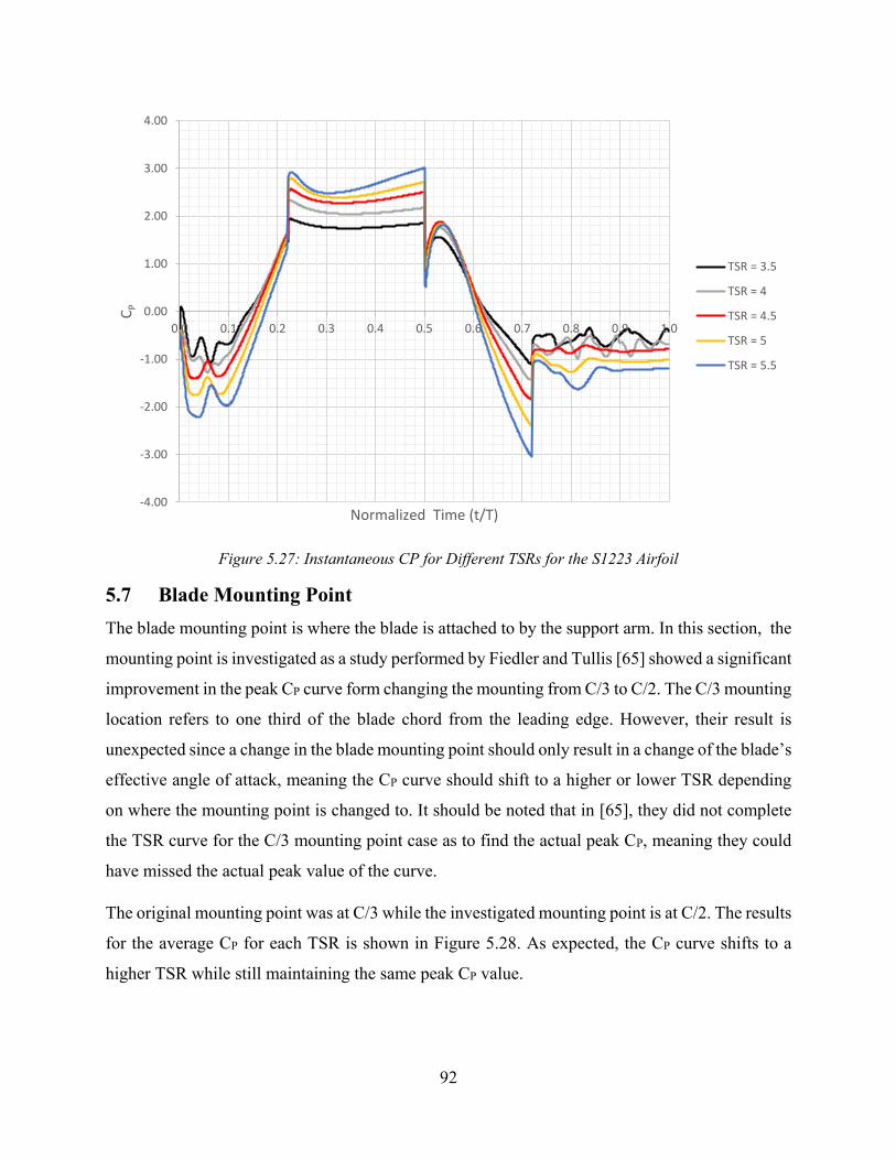
92

Figure 5.27: Instantaneous CP for Different TSRs for the S1223 Airfoil

5.7 Blade Mounting Point

The blade mounting point is where the blade is attached to by the support arm. In this section, the

mounting point is investigated as a study performed by Fiedler and Tullis [65] showed a significant

improvement in the peak CP curve form changing the mounting from C/3 to C/2. The C/3 mounting

location refers to one third of the blade chord from the leading edge. However, their result is

unexpected since a change in the blade mounting point should only result in a change of the blade’s

effective angle of attack, meaning the CP curve should shift to a higher or lower TSR depending

on where the mounting point is changed to. It should be noted that in [65], they did not complete

the TSR curve for the C/3 mounting point case as to find the actual peak CP, meaning they could

have missed the actual peak value of the curve.

The original mounting point was at C/3 while the investigated mounting point is at C/2. The results

for the average CP for each TSR is shown in Figure 5.28. As expected, the CP curve shifts to a

higher TSR while still maintaining the same peak CP value.

-4.00

-3.00

-2.00

-1.00

0.00

1.00

2.00

3.00

4.00

0.0 0.1 0.2 0.3 0.4 0.5 0.6 0.7 0.8 0.9 1.0

CP

Normalized Time (t/T)

TSR = 3.5

TSR = 4

TSR = 4.5

TSR = 5

TSR = 5.5

93

Figure 5.28: Average CP per Cycle vs TSR for Different Blade Mounting Points (MP)

The instantaneous CP can be seen in Figure 5.29, where similar trends are observed to the original

mounting point. The only difference is noticed in the upstream translational region, where the peak

is noticed to occur towards the end of the region instead of happening at start as previously seen.

Figure 5.29: Instantaneous CP for Different TSRs for the Blade Mounting Point at Half Chord

0.48

0.50

0.52

0.54

0.56

0.58

0.60

3 3.5 4 4.5 5 5.5 6 6.5

CP

TSR

MP at C/2

MP at C/3 (Original)

-1.00

-0.50

0.00

0.50

1.00

1.50

2.00

0.0 0.2 0.4 0.6 0.8 1.0

CP

Normalized Time (t/T)

TSR = 4

TSR = 4.5

TSR = 5

TSR = 5.5

TSR = 6

94

5.8 Summary and Discussion of Parametric Study

In this chapter, the TSR behavior of the original turbine was investigated as well as five other

parameters, including the incident wind angle, AEF, number of blades, airfoil profile and blade

mounting point. It was noticed that in general, the CP curve of the D-VAWT is not highly sensitive

to the change of TSR compared to most other wind turbines, which is another benefit of the D-

VAWT design. Through the incident wind angle study, it was confirmed that though the turbine

does indeed lose performance with incident wind angles other than zero, for a 40° range (± 20°) of

incident angles, the turbine loses only a maximum of 10% of its aerodynamic efficiency. From the

AEF study, it was found that increasing the AEF lead to a reduction of the peak CP, an increase in

the actual power output, and the CP curve becoming less sensitive to the change in TSR. By

studying a two bladed turbine with double solidity, it was found that the peak CP slightly increased

and the CP curve shifted to a lower TSR while also becoming more sensitive to the change of TSR.

From the study of a high lift cambered airfoil, it was confirmed that for D-VAWT application, the

camber will sacrifice the power on half of the cycle, leading to a significant loss in overall

aerodynamic efficiency. Finally, the mounting point study showed that it is possible to shift the CP

curve to a higher or lower TSR by modifying the blade mounting point, while still retaining the

original performance of the D-VAWT.

Since the analyses performed in this chapter constitute the preliminary analysis of the parametric

study, each parameter was investigated separately to help isolate each of their effects on the

performance. However, it is not possible to design a turbine based on a single parametric study,

but a multi-objective study is needed. For example, the wind sensitivity study showed that 10%

loss is sustained in aerodynamic efficiency for a 40° range, but this was done on an AEF of 4. The

losses could be greater or lower if one were to change the AEF value or perhaps add another blade.

Thus performing such parameter combinations is necessary as it is possible that the trends from

parameter combinations to behave differently from the ones predicted in the current analysis.

Performing such analyses can be extremely time consuming as there is a very large number of

possible cases that could be generated. This is why performing the current preliminary analysis

should help guide future designs of the D-VAWT and reduce the number of cases to a manageable

amount.

95

CHAPTER 6: CONCLUSION

6.1 Summary

Using CFD as the design tool, 2D simulations were used for the methodology validation

of the D-VAWT, while 3D simulations were used to obtain a more realistic performance

prediction. The validation of the methodology was performed for a single blade in 2D, where the

mesh convergence, domain size, turbulence model, 𝑦+ strategy, and blade motion prescription

were investigated. The methodology was also validated with experimental results of a static airfoil

in 2D. The SA Strain/Vorticity turbulence model was shown to be a lower bound estimate of the

coefficient of power while the SST k-ω turbulence model gave a more accurate prediction of the

performance.

The novelty of the D-VAWT design is that it is among the few studies that modified a

turbine’s blade path in an attempt to improve the aerodynamic efficiency. In this thesis, it was

shown that the D-VAWT design did indeed succeed at improving the aerodynamic efficiency of

small scale turbines which has been a challenge to overcome for many decades. The performed

tests have shown the great potential of the D-VAWT by reporting a high CP performance of 0.4

for AR = 15 based on the 3D simulation. For a common straight blade Darrieus type turbine,

a CP of 0.4 is very high and difficult to achieve. However, the proposed D-VAWT is still far from

being fully optimized. It is also important to note that because the D-VAWT requires the wind to

be perpendicular to its longitudinal side to have optimal performance, this turbine now becomes

dependent on wind direction, which is a drawback not encountered in traditional VAWTs.

A preliminary parametric study was performed, where it was found that the D-VAWT has

a low sensitivity to the change of TSR compared to most other wind turbines. The incident wind

angle study showed that a maximum of 10% aerodynamic efficiency is lost for a ± 20° range of

incident angles while a maximum of 40% aerodynamic efficiency is lost for a ± 60° range of

incident angles. The AEF study showed that increasing the AEF will lower the peak CP, increase

power output, and reduce the TSR sensitivity. By studying a two bladed turbine, it was shown that

the D-VAWT maintained its high performance while reducing its TSR value at peak performance

and increasing its sensitivity to TSR change. Cambered airfoils were shown to reduce the overall

96

performance of D-VAWTs. Finally, the blade mounting point study showed no improvement in

performance but a shift in TSR at peak performance is possible.

6.2 Contributions

The following is the list of contributions of this thesis:

Proving the D-VAWT concept and performing a preliminary parametric study of design

variables;

Developing three moving mesh techniques to model the motion of a D-VAWT;

Comparison of different turbulence models for D-VAWT applications.

6.3 Future Work

Future studies will continue the investigation of the D-VAWT to further understand the

flow and turbine behavior for different geometrical parameters and operating conditions. Future

studies can still be performed in 2D as the trends and behaviors predicted will still be valid for

future designs, while the results can be obtained in a matter of days instead of months. A more in-

depth parametric analysis is required to optimize the D-VAWT. This will also require a multi-

objective study where more than one parameter is modified at once since the behavior from the

parameter combinations could result in new trends. For example, one should combine the AEF

with the incident wind angles study or the AEF study with multiple blades. More analyses are

required for more multi-blade type D-VAWTs as a turbine with a single and two blades were

simulated. However, the additional blades will create more interaction between all the blades and

the flow, which require further simulations to comprehend that said interaction.

The dimensions of the turbine should be also investigated as only a single turbine size was

investigated in this study. This should be done in conjunction with a structural analysis to obtain

a viable design. The mechanism of the D-VAWT will also need to be designed and included in the

structural analysis.

One interesting concept will be to simulate a turbine with variable TSR in a cycle. Since

the D-VAWT’s translating regions operated more efficiently at high TSR, while the rotating

regions operated more efficiently at low TSR, combining a high and low TSR value in one cycle

could result in much more aerodynamically efficient turbine. The difficulty will be designing a

mechanism to account for a variable TSR during the blade rotation.

97

Once a complete design is obtained from future 2D investigations, a full scale 3D

simulation, without the symmetry condition, should be performed with an atmospheric velocity

inlet boundary condition to obtain an even more realistic estimate of its performance. Also, to

obtain even more realistic results, one should simulate the D-VAWT mechanism as it will add

additional drag and fluid-structure interactions (FSI) with the blades as well as using a 6 degree of

freedom (DOF) type simulation in Fluent to consider the inertia of the components. The D-VAWT

is not limited to urban applications. It can be used on a much larger scale in the field outside cities,

however, the large scale version of the D-VAWT will also require investigation to ensure its

optimal performance.

Since the D-VAWT requires the wind to be normal to its longitudinal side for optimal

performance, combining the D-VAWT with a shroud could help align the flow in the desired

direction. The shroud should provide the D-VAWT with a larger operating range of incident wind

angles. The other solution to help with the wind dependency problem is a mechanical solution,

where one of the two axes is allowed to pivot so that the flow is always normal to the longitudinal

side of the turbine. Both solutions are viable and require further investigation.

With the D-VAWT concept proven, it is also possible to investigate a turbine with different

blade paths such as one with a triangular shape with three axes to make the turbine performance

even less sensitive to wind direction. Finally, a study where one combines the D-VAWT with the

morphing blade technology to maximize the airfoil’s lift potential throughout the entire blade path

could be interesting to investigate.

6.3.1 Future Work Summary

Perform a multi-objective parametric study and optimization.

Investigate the D-VAWT for different sizes and develop its mechanism.

Study a case with variable TSR in a cycle (i.e. High TSR in translational region and low

TSR in rotating regions).

Perform full 3D simulations with atmospheric inlet velocity, multiple blades, and

mechanical components.

Combine the D-VAWT with a shroud or axis pivotal system.

Investigate new blade paths such as a triangular shaped path.

Investigate morphing blade technology with the D-VAWT.

98

REFERENCES

[1] OECD and IEA, “Key World Energy Statistics,” IEA Publishing, Paris, 2015.

[2] Natural Resources Canada, “Energy Fact Book,” 2015-2016.

[3] Global Wind Energy Council, “Global Wind Report - Annual Market Update,” Brussles,

2015.

[4] World Wind Energy Association, J.-D. Pitteloud, and S. Gsanger, “Small Wind World

Report,” Tokyo, 2016.

[5] Reve, “Siemens Provides 157 Wind Turbines for Three Wind Power Projects in South

Africa.” [Online]. Available: http://www.evwind.es/2015/02/18/siemens-provides-157-

wind-turbines-for-three-wind-power-projects-in-south-africa/50574. [Accessed: 23-Jul-

2016].

[6] Québec en Saisons, “Découvrez les secrets de «Éole Cap-Chat».” [Online]. Available:

http://www.quebecensaisons.com/ete2009/eole_cap_chat.php. [Accessed: 23-Jul-2016].

[7] R. D, “Vertical Axis Wind Turbine Installed in P-Town.” [Online]. Available:

http://www.alternativeconsumer.com/2009/06/30/vertical-axis-wind-turbine-installed-in-

p-town/. [Accessed: 23-Jul-2016].

[8] Quiet Revolution, “The qr6 Vertical Axis Wind Turbine.” [Online]. Available:

http://www.quietrevolution.com/. [Accessed: 23-Jul-2016].

[9] Wind Harvest International, “WHI 70 kW.” [Online]. Available:

http://www.windharvest.com/. [Accessed: 23-Jul-2016].

[10] P. Kozak, “Effects of Unsteady Aerodynamics on Vertical-Axis Wind Turbine

Performance,” MS Thesis, Dept. of Mech. and Aero. Eng., Illinois Institute of Technology,

Chicago, Ill., 2014.

[11] S. Eriksson, H. Bernhoff, and M. Leijon, “Evaluation of different turbine concepts for wind

power,” Renewable Sustainable Energy Rev., vol. 12, no. 5, pp. 1419–1434, 2008.

[12] R. Guillo, “Darrieus vertical axis wind turbine.” [Online]. Available:

http://www.ecosources.info/en/topics/Darrieus_vertical_axis_wind_turbine. [Accessed:

02-Feb-2016].

[13] E. Hau, Renewable Energy, Fundamental, Technology, Applications and Economics, Berlin

Heidelberg. Springer-Verlag, 2006.

[14] Gamma Energy, “Teoria delle turbine eoliche.” [Online]. Available:

http://www.gammaenergy.it/eolico/teoria-delle-turbine.html. [Accessed: 07-Jul-2016].

[15] I. Paraschivoiu, Wind Turbine Design with Emphasis on Darrieus Concept. Montreal:

Presse Internationales Polytechniques, 2002.

99

[16] S. N. Zadeh, M. Komeili, and M. Paraschivoiu, “Mesh Convertence Study for 2-D Straight-

Blade Vertical Axis Wind Turbine Simulations and Estimation for 3-D Simulations,” Can.

Scociety Mech. Eng., vol. 38, no. 4, pp. 487–504, 2014.

[17] ANSYS Inc., 2011. ANSYS FLUENT 14.0 User’s Guide, URL: www.fluent.com.

[18] X. Jin, G. Zhao, K. Gao, and W. Ju, “Darrieus vertical axis wind turbine: Basic research

methods,” Renewable Sustainable Energy Rev., vol. 42, pp. 212–225, 2015.

[19] F. L. Ponta, J. J. Seminara, and A. D. Otero, “On the aerodynamics of variable-geometry

oval-trajectory Darrieus wind turbines,” Renewable Energy, vol. 32, no. 1, pp. 35–56, 2007.

[20] F. L. Ponta and L. I. Lago, “Analysing the suspension system of variable-geometry oval-

trajectory (VGOT) Darrieus wind turbines,” Energy Sustain. Dev., vol. 12, no. 2, pp. 5–16,

2008.

[21] T. Kinsey and G. Dumas, “Computational Fluid Dynamics Analysis of a Hydrokinetic

Turbine Based on Oscillating Hydrofoils,” ASME J. Fluids Eng., vol. 134, no. 2, p. 021104,

2012.

[22] T. Kinsey and G. Dumas, “Three-Dimensional Effects on an Oscillating-Foil Hydrokinetic

Turbine,” ASME J. Fluids Eng., vol. 134, no. 7, p. 071105, 2012.

[23] T. Kinsey, G. Dumas, G. Lalande, J. Ruel, a. Méhut, P. Viarouge, J. Lemay, and Y. Jean,

“Prototype testing of a hydrokinetic turbine based on oscillating hydrofoils,” Renewable

Energy, vol. 36, no. 6, pp. 1710–1718, 2011.

[24] É. Gauthier, T. Kinsey, and G. Dumas, “Impact of blockage on the hydrodynamic

performance of oscillating-foils hydrokinetic turbines,” vol. 138, no. 9, p. 091103, 2016.

[25] P. Delafin, T. Nishino, L. Wang, A. Kolios, and T. Bird, “Comparison of RANS CFD and

lower-order aerodynamic models for 3D Vertical Axis Wind Turbines,” Eur. Wind Energy

Conf. Exhib., 2015.

[26] M. H. Mohamed, A. M. Ali, and A. A. Hafiz, “CFD analysis for H-rotor Darrieus turbine

as a low speed wind energy converter,” Eng. Sci. Technol. an Int. J., vol. 18, no. 1, pp. 1–

13, 2015.

[27] W. Yamazaki and Y. Arakawa, “Inexpensive airfoil shape optimization for vertical axis

wind turbine and its validation,” J. Fluid Sci. Technol., vol. 10, no. 2, 2015.

[28] Q. Xiao, W. Liu, and A. Incecik, “Flow control for VATT by fixed and oscillating flap,”

Renewable Energy, vol. 51, pp. 141–152, 2013.

[29] Y. C. Lim, W. T. Chong, and F. B. Hsiao, “Performance investigation and optimization of

a vertical axis wind turbine with the omni-direction-guide-vane,” Procedia Eng., vol. 67,

pp. 59–69, 2013.

[30] W. T. Chong, A. Fazlizan, S. C. Poh, K. C. Pan, W. P. Hew, and F. B. Hsiao, “The design,

simulation and testing of an urban vertical axis wind turbine with the omni-direction-guide-

vane,” Appl. Energy, vol. 112, pp. 601–609, 2013.

[31] R. Gosselin, G. Dumas, and M. Boudreau, “Parametric study of H-Darrieus vertical-axis

100

turbines using uRANS simulations,” 21st Annu. Conf. CFD Soc. Canada, vol. 178, 2013.

[32] F. Balduzzi, A. Bianchini, R. Maleci, G. Ferrara, and L. Ferrari, “Critical issues in the CFD

simulation of Darrieus wind turbines,” Renewable Energy, vol. 85, pp. 419–435, 2016.

[33] P. Chatterjee and R. N. Laoulache, “Performance Modeling of Ducted Vertical Axis

Turbine Using Computational Fluid Dynamics,” Mar. Technol. Soc. J., vol. 47, no. 4, 2013.

[34] A. Untaroiu, H. G. Wood, P. E. Allaire, and R. J. Ribando, “Investigation of Self-Starting

Capability of Vertical Axis Wind Turbines Using a Computational Fluid Dynamics

Approach,” J. Sol. Energy Eng., vol. 133, no. 4, p. 041010, 2011.

[35] M. R. Castelli, A. Englaro, and E. Benini, “The Darrieus wind turbine: Proposal for a new

performance prediction model based on CFD,” Energy, vol. 36, no. 8, pp. 4919–4934, 2011.

[36] M. R. Castelli, G. Pavesi, L. Battisti, E. Benini, and G. Ardizzon, “Modeling Strategy and

Numerical Validation for a Darrieus Vertical Axis Micro-Wind Turbine,” Int. Mech. Eng.

Congr. Expo., vol. Vol. 7, no. IMECE2010–39548, pp. 409 – 418, 2010.

[37] F. Trivellato and M. Raciti Castelli, “On the Courant-Friedrichs-Lewy criterion of rotating

grids in 2D vertical-axis wind turbine analysis,” Renewable Energy, vol. 62, pp. 53–62,

2014.

[38] M. H. Mohamed, “Performance investigation of H-rotor Darrieus turbine with new airfoil

shapes,” Energy, vol. 47, no. 1, pp. 522–530, 2012.

[39] R. Howell, N. Qin, J. Edwards, and N. Durrani, “Wind tunnel and numerical study of a

small vertical axis wind turbine,” Renewable Energy, vol. 35, no. 2, pp. 412–422, 2010.

[40] H. Beri and Y. Yao, “Effect of Camber on Airfoil on Self Starting of Vertical Axis Wind

Turbine,” J. Environ. Sci. Technol., vol. 4, no. 3, pp. 302–312, 2011.

[41] B. Yang and C. Lawn, “Fluid dynamic performance of a vertical axis turbine for tidal

currents,” Renewable Energy, vol. 36, no. 12, pp. 3355–3366, 2011.

[42] T. Maître, E. Amet, and C. Pellone, “Modeling of the flow in a Darrieus water turbine: Wall

grid refinement analysis and comparison with experiments,” Renewable Energy, vol. 51,

pp. 497–512, 2013.

[43] S. Lain and C. Osorio, “Simulation and evaluation of a straight-bladed darrieus-type cross

flow marine turbine,” J. Sci. Ind. Res. (India)., vol. 69, no. 12, pp. 906–912, 2010.

[44] A. Rossetti and G. Pavesi, “Comparison of different numerical approaches to the study of

the H-Darrieus turbines start-up,” Renewable Energy, vol. 50, pp. 7–19, 2013.

[45] C. J. S. Ferreira, H. Bijl, G. van Bussel, and G. van Kuik, “Simulating Dynamic Stall in a

2D VAWT: Modeling strategy, verification and validation with Particle Image Velocimetry

data,” J. Phys. Conf. Ser., vol. 75, p. 012023, 2007.

[46] J. McNaughton, F. Billard, and a. Revell, “Turbulence modelling of low Reynolds number

flow effects around a vertical axis turbine at a range of tip-speed ratios,” J. Fluids Struct.,

vol. 47, pp. 124–138, 2014.

101

[47] R. Lanzafame, S. Mauro, and M. Messina, “2D CFD modeling of H-Darrieus Wind

Turbines using a transition turbulence model,” Energy Procedia, vol. 45, pp. 131–140,

2014.

[48] M. S. Siddiqui, N. Durrani, and I. Akhtar, “Quantification of the effects of geometric

approximations on the performance of a vertical axis wind turbine,” Renewable Energy, vol.

74, pp. 661–670, 2015.

[49] M. R. Castelli, A. D. Monte, M. Quaresimin, and E. Benini, “Numerical evaluation of

aerodynamic and inertial contributions to Darrieus wind turbine blade deformation,”

Renewable Energy, vol. 51, pp. 101–112, 2013.

[50] S. M. Salim and S. C. Cheah, “Wall y + Strategy for Dealing with Wall-bounded Turbulent

Flows,” Int. MultiConference Eng. Comput. Sci., vol. II, 2009.

[51] K. M. M. Almohammadi, D. B. B. Ingham, L. Ma, and M. Pourkashan, “Computational

fluid dynamics (CFD) mesh independency techniques for a straight blade vertical axis wind

turbine,” Energy, vol. 58, pp. 483–493, 2013.

[52] T. Lee and Y. Y. Su, “Surface Pressures Developed on an Airfoil Undergoing Heaving and

Pitching Motion,” ASME J. Fluids Eng., vol. 137, no. 5, pp. 1–11, 2015.

[53] J. Dacles-Mariani, G. G. Zilliac, J. S. Chow, and P. Bradshaw, “Numerical Simulations of

a Wingtip Vortex in the Near Field,” AIAA J., vol. 33, no. 9, pp. 1561–1568, 1995.

[54] J. Dacles-Mariani, D. Kwark, and G. G. Zilliac, “On numerical errors and turbulence

modeling in tip vortex flow prediction,” Int. J. Numer. Methods Fluids, vol. 30, pp. 65–82,

1999.

[55] ANSYS Inc., 2011. ANSYS FLUENT 14.0 Theory Guide, URL: www.fluent.com.

[56] M. F.R., “Two-equation eddy-viscosity turbulence models for engineering applications,”

AIAA J., vol. 32–8, no. 8, pp. 1598–1605, 1994.

[57] F. R. Menter, M. Kuntz, and R. Langtry, “Ten Years of Industrial Experience with the SST

Turbulence Model,” Turbul. Heat Mass Transf. 4, vol. 4, pp. 625–632, 2003.

[58] F. R. Menter, R. B. Langtry, S. R. Likki, Y. B. Suzen, P. G. Huang, and S. Völker, “A

Correlation-Based Transition Model Using Local Variables—Part I: Model Formulation,”

J. Turbomach., vol. 128, no. 3, pp. 413–422, 2004.

[59] R. B. Langtry, F. R. Menter, S. R. Likki, Y. B. Suzen, P. G. Huang, and S. Völker, “A

Correlation-Based Transition Model Using Local Variables—Part II: Test Cases and

Industrial Applications,” J. Turbomach., vol. 128, no. 3, p. 423, 2006.

[60] I. Paraschivoiu, Aérodynamique Subsonique. Montreal Canada: Ed. École Polytechnique,

1998.

[61] G. Naccache and M. Paraschivoiu, “Two Dimensional Flow Simulations of a Dual Axis

Wind Turbine,” in EIC Climate Change Technology Conference, 2015.

[62] P. J. Roache, “Perspective: A method for Uniform Reporting of Grid Refinement Studies,”

ASME J. Fluids Eng., vol. 158, pp. 109–121, 1993.

102

[63] W. A. Timmer, “Two-dimensional low-Reynolds number wind tunnel results for airfoil

NACA 0018,” Wind Eng., vol. 32, no. 6, pp. 525–537, 2009.

[64] M. S. Selig and J. J. Guglielmo, “High-Lift Low Reynolds Number Airfoil Design,” J.

Aircr., vol. 34, no. 1, pp. 72–79, 1997.

[65] A. J. Fiedler and S. Tullis, “Blade Offset and Pitch Effects on a High Solidity Vertical Axis

Wind Turbine,” Wind Eng., vol. 33, no. 3, pp. 237–246, 2009.