cfd multi-phase flow analysis across diverging manifolds

CFD MULTI-PHASE FLOW ANALYSIS ACROSS DIVERGING MANIFOLDS:APPLICATION IN THE OIL-GAS INDUSTRY

Sergio Croquer, M.Sc.Department of Energy Conversion and Transport

Universidad Simon BolivarSartenejas, Venezuela. 01080

Email: [email protected]

Joaquin Vieiro, M.Sc.Department of Energy Conversion and Transport



Carlos Chacon, M.Sc.Department of Mechanical SystemsUniversidad Simon Bolivar - Litoral

Camuri, Venezuela. 01080Email: [email protected]

Miguel Asuaje, Ph.D.Department of Energy Conversion and Transport



ABSTRACT

This investigation assessed detailed characteristics of flowin diverging manifolds, for water and water-oil cases. A 3DComputational Fluid Dynamics (CFD) model of a distributingmanifold was carried out. Numerical results showed goodagreement with experimental values. Predicted pressure andvelocity contours agree with theory, detailed 3D insight onpresent secondary flows and localized hydraulic losses wasobtained, as well as effect on distribution of phases. Moreover,a 3D, multi-phase (oil-water) CFD model of a divergingmanifold design, similar to those installed in separation unitswas conducted. The main pipe had 0.762 m (30 in) indiameter and 24 m in length, with 8 perforated pipes branchingout. Branches had 0.305 m (12 in) in diameter and 12 min length, with 312 holes per branch. Non-uniform outflowdistributions were detected, as well as secondary flows. Analternate design was proposed. Numerical results show the newmanifold design achieves uniform static pressure distributionacross the entire main pipe, reducing secondary flows andhydraulic losses. Outflow distribution is also uniform, thusimproving the performance of the separation unit.

NOMENCLATUREd Branch diameter [m].D Main pipe diameter [m].h Branch length [m].Nbranches Number of Branches [-].Or Outflow ratio. Eq. 1 [-].RMS Root Mean Square [-]S Distance between consecutive branches [m].qi Flow exiting through branch i [kg/s]qbranch Outflow through each branch [kg/s]. Eq. 5.Qin Flow entering the manifold [kg/s].Vf ,phase Volume fraction for phase [-]. Eq. 4.Vmax Maximum desired flow velocity [kg/s].

INTRODUCTIONDiverging manifolds are widely use in the industry. Many

operations, at different scales, require the proper distribution ofa flowstream into various derivations, e.g.: intake of internalcombustion engines, heat exchangers and air conditioningsystems [1–3]. In the oil & gas industry, pipe manifoldsare used to consolidate outflow of different wells, in pumping

Proceedings of the ASME 2014 International Mechanical Engineering Congress and Exposition IMECE2014

November 14-20, 2014, Montreal, Quebec, Canada

IMECE2014-36681

1 Copyright © 2014 by ASME

and compression stations, and as inlet system to differentequipment. In large volume gravity separation tanks, pipemanifolds with perforated branches are used as feed distributionsystems (similar to a shower head). In this case, inlet flowuniformity is important to prevent high velocity regions andincrease separation performance.

Figure 1 depicts a typical divergent manifold, witha constant diameter main pipe. Characteristic geometricparameters of this design are: Main pipe diameter (D), branchpipes diameter (d), distance between branches (s) and length ofbranches (h). In this study, branches are numbered according tothe sequence in which the flow reaches each of them.

Although the construction of these pipe systems might seemeasy, circulating flow is complex and might lead to increasedhydraulic losses. One dimensional hydraulic theory shows thatfor a main pipe of constant diameter, mean velocity along theprincipal line diminishes as flow is drawn into the branchingtubes [4], [5]. Static pressure along the main line thus increases,resembling a diffusive process.

This behavior has been verified both through experimentalobservations and numerical simulations. Experimental analysescarried out by Acrivos et al. [6] show sudden rises in pressureafter each leaving branch. While, between branches, pressuredecreases due to energy losses. Hence, the resulting profilealong the main pipe adopts an escalated ascending form, reachingvalues above the inlet pressure condition.

Others experiments showed sudden changes in main flowinto the branches lead to uneven outflow ratio 1. Experimentalstudies carried out on a constant diameter manifold with 10leaving branches, show a constant increase in outflow ratio, from9% in the first branch to above 14% in the last [7].

The outflow ratio is defined as the proportion of flow leavingeach branch to the intake:

Ori =qi

Qin(1)

Numerical models, based on one dimensional (1D) Navier-Stoke (NS) equations, and empiric relationships for losscoefficients have been carried out [3, 8]. Despite beingquite simple, this methods show very good agreement versusexperimental values. Allowing an accurate prediction of globalparameters across the manifold (outflow distribution, pressurealong the main pipe).

CFD studies in 2D showed the influence of differentgeometric parameters such as the area ratio (d/D), and s overflow distribution and losses [9]. Other CFD analyses have beencarried out to asses the effect of particular manifold designs oninternal combustion engines, or heat exchangers [2, 10]

The objective of this investigation was to provide insightful

FIGURE 1. TYPICAL DIVERGENT MANIFOLD WITHCONSTANT DIAMETER (D) MAIN PIPE.

information regarding the complex phenomena appearing indiverging manifolds, by carrying out a three dimensional, multi-phase, CFD analysis of two different distribution systems.

The first model (cases 1a-1e) was meant to replicateexperimental data provided by [7]; assess different boundaryconditions; and predict the effect of including a two-phasemixture (water-oil).

The second model (cases 2a-2e) was based on a divergingmanifold currently used in the oil & gas industry. Thismodel comprised perforated branches, and an oil in wateremulsion as working fluid. Four manifold prototypes withprogressive reductions in main pipe diameter were analyzed.The design steps for these improved manifolds are outlined inthe Methodology section. All models were developed usingANSYS® CFX® v.14.

METHODOLOGYFor the first parts (cases 1a-1e), the experimental study by

Kubo & Ueda [7] was chosen, as it provided enough data todevelop a representative numerical model. Once this model wasvalidated against experimental results, two-phase calculations(water-oil) were carried out to asses the influence of oil volumefraction (Vf ) on manifold performance.

The second model (cases 2a-2e) was based on an actualdiverging manifold, currently installed in an oil-water separationfacility. This was a two-phase (oil-water), 3D model. Alternativedesigns, with progressive reductions in the main pipe diameter,were evaluated for performance, pressure drops, and outflowratio distribution. Table 1 resumes all studied cases.

Governing EquationsThe CFD models were constructed using the commercial

package ANSYS CFX v14. This suite solves a discretizedform of the flow conservative governing equations for eachmesh volume (following the finite volume approach) [11].The flows investigated in this paper were steady, isothermal,incompressible, liquids. Hence, the main solved equations werecontinuity (2) and momentum in the three principal directions


TABLE 1. SUMMARY OF CASES PRESENTED IN THIS PAPER.

Case No. Description

1a Single phase (water), replicatingdata by [7]. Static Pressure at Inlet,Mass Flow at Outlets.

1b Single phase (water), replicatingdata by [7]. Total mass flow at Inlet,Static pressure at Outlets.

1c-1e Two phase (water-oil), effect ofincreasing oil concentration on theperformance of manifold in case 1a.

2a Current Water-oil, current manifold.Main pipe of constant diameter.Perforated branches.

2b - 2e Proposed Water-oil, proposed manifolds.Main pipe with progressivediameter reductions. Perforatedbranches.

(3).

∂ρ

∂ t+∇• (ρ~U) = 0 (2)

∂

(ρ~U)

∂ t+∇•

(ρ~U ×~U

)=−∇p+∇• τ + ~SM (3)

The selected turbulence model was κ - ε , and closurerelationships for these terms are also computed. The two-phaseflow was considered non-homogeneous in terms of the fieldvelocity, thus separate continuity and momentum equations aresolved for each phase.

The oil phase was considered a dispersed fluid composedof spheric particles of constant diameter. Momentum transferacross fluids in ANSYS CFX v14 is considered to result fromthe contribution of different fluid interaction forces such as lift,drag, etc. These are calculated as function of the particles shape,fluids contact area, and fluid velocities [11]

Cases 1a-1b - Single Phase ModelSimulation Domain The first model was a single phase

(water), 3D, CFD computation of a manifold with constant pipediameter and 10 branches. The objective of this model was to

TABLE 2. GEOMETRIC PARAMETERS OF THE SINGLE-PHASE MODEL (BASED ON [7]).

Parameter Value

Main Pipe Diameter (D) [m] 0.02

Branch Diameter (d) [m] 0.01

Distance between branches (s) [m] 0.06

Length of branches (h) [m] 0.8

FIGURE 2. SPATIAL DISCRETIZATION FOR THE SINGLE-PHASE MODEL. (a) SURFACE MESH NEAR ONE OF THEBRANCH JUNCTIONS. (b) DETAIL IN A CROSS SECTIONALSLICE.

reproduce the data given by [7]. Table 2 resumes geometricparameters of this manifold, as defined in Figure 1.

The spatial grid was built using ANSYSWorkbench™Meshing Tool. It consisted of 4 MM tetrahedralelements and 1.6 MM nodes. Maximum face size was set to 0.04m. Inflation layers were set on all the walls to better reproducewall effects. A slight reduction in element size was set inthe areas were branches parted from the main pipe. With thisconfiguration, over 95% of the elements had an Aspect Ratiounder 10. Figure 2 depicts a region of the surface mesh near oneof the branches, as well as a cross sectional plane of the mesh.

Boundary Conditions For the single-phase model, twosets of boundary conditions were tested in order to assess theiraccuracy. In Case 1a: static pressure was fixed at the inlet, andleaving mass flow at each branch was set according to data givenby [7]. For Case 1b boundary conditions were reversed: totalmass flow was fixed at the inlet, and uniform static pressure wasimposed at all exits (101.325 kPa). For both models, a non-slip wall condition was defined on every pipe surface. Figure 3depicts the location of boundary conditions.


FIGURE 3. BOUNDARY CONDITIONS SET FOR THE SINGLEPHASE MODEL.

Numerical Parameters For the single phase model,water was considered an incompressible fluid with constantproperties at 298 K. In this case, only 6 equations needed to besolved: continuity, momentum (X,Y,Z), and transport equationsfor turbulent kinetic energy (κ), and turbulent dissipation(ε) [12]. Computations were carried out in steady state regime(neglecting the time derivative). The convective term in thetransport equations was computed with a 2nd order scheme.Given its low computational cost and numerical stability, theκ − ε model, with scalable wall function, was chosen forturbulence modeling. Previous works have used this modelon manifolds, obtaining a good compromise between resultsand performance [9]. Convergence criteria were: momentumresiduals RMS under 1E-4 and mass imbalances under 1%.

Cases 1c-1d - Two-Phase ModelCases 1c trough 1e were computed with the same domain,

mesh and boundary conditions of case 1a. For this two-phasemodel, the fluids were water as incompressible liquid at 298K and oil as disperse constant diameter droplets. Table 3summarizes oil phase characteristics. These data were obtainedfrom field reports of an operating facility in South America, anddifferent correlations [13].

Boundary Conditions and Numerical ParametersThe boundary condition set for models 1c-1e was the same asin case 1a (Static Pressure at inlet, mass flow at exits). Phasedistribution was defined in terms of the volume fraction (Vf ):

Vf ,phase =Vphase

Vtotal(4)

TABLE 3. PROPERTIES OF THE OIL PHASE.

Property Value

Morphology Constant diameter droplets

Droplet Diameter [mm] 1.934

Density [kg/m3] 978

Viscosity [Pa s] 7.8E-6

For cases 1c, 1d and 1e, inlet oil Vf values were: 5%, 10%and 20% respectively.

The multi-phase fields were computed with the non-homogeneous model. In this model, X-Y-Z momentumequations are solved separately for each phase. The interactionbetween fluids (e.g.: momentum transfer) was accounted viainter-phase transfer coefficients. The drag coefficient is thencalculated accordingly, using the particle model of ANSYS CFXv14 [11].

Other numerical settings (advection scheme, turbulencemodel, convergence criteria) were the same as those in the single-phase model.

Cases 2a-2e - Reducing Diameter ManifoldSimulation Domain Case 2a reflects the design of a

diverging manifold currently used as inlet system in a largevolume gravity separation tank. For this case, the main pipe had aconstant nominal diameter of 0.762 m (30 in) and a its length was24 m. The manifold had 8 perforated pipes as branches [nominaldiameter 0.305 m (12 in), length 12 m], with 312 holes of 0.012m (1/2 in) distributed in crowns of 8 holes each.

Cases 2b to 2e represent proposed manifold designs. Theobjective of these models was to mitigate the uneven outflowdistribution and pressure rises of case 2a, by promoting a uniformmean velocity along the main pipe. For cases 2b and 2c, leavingbranches had a nominal diameter of 0.254 m (10 in) and 12 min length, with orifices of 0.016 m (5/8 in). For cases 2d and 2e,branches had a nominal diameter of 0.305 m (12 in) and orificeshad a diameter of 0.012 m (1/2 in).

Figure 4 compares the variations in main pipe diameteracross cases 2a to 2e.

For models 2a-2e, spatial grids were generated followingthe same principles as in cases 1a and 1b. Since the modelsin this section were much bigger, maximum element face wasset to 0.1 m. However, a minimum element size of 0.0075m was established at the orifices to ensure they were correctlydiscretized. Figure 5 depicts details of one of these meshes. Inaverage, these had 6.5 MM elements and 1.9 MM nodes.


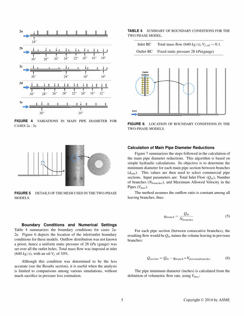
FIGURE 4. VARIATIONS IN MAIN PIPE DIAMETER FORCASES 2a - 2e.

FIGURE 5. DETAILS OF THE MESH USED IN THE TWO-PHASEMODELS.

Boundary Conditions and Numerical SettingsTable 4 summarizes the boundary conditions for cases 2a-2e. Figure 6 depicts the location of the inlet/outlet boundaryconditions for these models. Outflow distribution was not knowna priori, hence a uniform static pressure of 28 kPa (gauge) wasset over all the outlet holes. Total mass flow was imposed at inlet(640 kg/s), with an oil Vf of 10%.

Although this condition was determined to be the lessaccurate (see the Results section), it is useful when the analysisis limited to comparisons among various simulations, withoutmuch sacrifice in pressure loss estimation.

TABLE 4. SUMMARY OF BOUNDARY CONDITIONS FOR THETWO PHASE MODEL.

Inlet BC Total mass flow (640 kg/s), Vf ,oil = 0.1.

Outlet BC Fixed static pressure 28 kPa(gauge)

FIGURE 6. LOCATION OF BOUNDARY CONDITIONS IN THETWO-PHASE MODELS.

Calculation of Main Pipe Diameter ReductionsFigure 7 summarizes the steps followed in the calculation of

the main pipe diameter reductions. This algorithm is based onsimple hydraulic calculations. Its objective is to determine theminimum diameter for each main pipe section between branches(dmin). This values are then used to select commercial pipesections. Input parameters are: Total Inlet Flow (Qin), Numberof branches (Nbranches), and Maximum Allowed Velocity in thePipes (Vmax).

The method assumes the outflow ratio is constant among allleaving branches, thus:

qbranch =Qin

Nbranches(5)

For each pipe section (between consecutive branches), theresulting flow would be Qin minus the volume leaving in previousbranches:

Qsection = Qin −qbranch ∗Npreviousbranches (6)

The pipe minimum diameter (inches) is calculated from thedefinition of volumetric flow rate, using Vmax:


FIGURE 7. STEPS FOR THE SELECTION OF VARIABLE PIPEDIAMETERS.

Dmin =

√4.Qsection

πVmaxx

1in0.0254m

(7)

If the value in SI units is desired, the conversion factor mustbe ignored. This result is then used to select correspondentcommercial pipes in the preferred schedule.

For the perforated pipes, minimum diameter was calculatedusing Eq 7.

Minimum diameter of the orifices was computed using totalleaving flow (Qin), number of orifices (Nori f ices) and Vmax:

dmin,ori f ices =

√4. Qin

Nori f ices

πVmaxx

1in0.0254m

(8)

This method was used in the design of manifolds for models2b - 2e. Such prototypes differ in number of size reductions andthe connection between the main pipe and the last branch, eitheran elbow (2b-2c) or a t-junction (2d-2e).

RESULTS - CASES 1a - 1eValidation Against Experimental Values

Figure 8 compares outflow ratio (qi/Qin) for cases 1a and1b vs. experimental values reported by [7]. For case 1a, outlet

FIGURE 8. SINGLE-PHASE MODEL VALIDATION. Ori PERBRANCH

FIGURE 9. SINGLE-PHASE MODEL VALIDATION. PRESSUREPROFILE ALONG MAIN PIPE LINE. CASES 1a & 1b.

mass flows were computed directly from experimental values [7],hence good agreement is expected.

For case 1b, the model predicts an even outflow distributionacross all branches. Hence, outflow ratios for branches 1-4are overestimated, and for branches 6-10 are underestimated.Maximum deviation from experimental results occurs at the 1st

branch (40%).

Figure 9 depicts evolution of static pressure along thepipeline respect to the value just before the 1st branch. Despitedifferences in outflow distribution, both numerical models showgood agreement respect to reference data after the 5th branch.For case 1a, predicted values deviated 2% - 13% from referencedata. Case 1b showed good agreement (under 10%) for branches5 to 10. For 1st and 2nd branches, results went away 58% and33% respectively.

The difference in pressure profiles, between numericalcomputations and the reference values [7] are probably due tothe smooth pipe wall assumption and the scalable wall functionof the turbulence model. Experimental uncertainties should alsobe considered.


FIGURE 10. VELOCITY FIELDS FOR CASES 1a & 1b.

Effect of different Boundary ConditionsFigure 10 shows the velocity field for cases 1a and 1b.

Along the main pipe, both profiles are very much alike. Alongthe branches, model 1a predicts the fluid leaving trough the 1st

branch will move much slower than in the last branch. The model1b predicts similar flow velocities across all branches.

Figure 11 details velocity vectors at junctions of branches1 and 10 for cases 1a and 1b. For the 1st branch, meanflow velocity in the main pipe is high enough that recirculationappears. Effective flow area for the outgoing flow is reduced,thus diminishing the outflow ratio and increasing energy losses.This behavior was observed in branches 1 through 8.

At branch 10, most of the flow has left the manifold in theprevious pipes, hence mean velocity in the mean pipe is verylow and there is no recirculation despite the sudden change indirection. As flow through the 10th branch in case 1a is greaterthan in case 1b, mean flow velocity is also greater.

Effect of Oil VfOil distribution, as volume fraction, is shown in Figure 12

for cases 1c-1e. According to these results, oil flowing inthe branches tends to stay near the walls. For the biggestinlet oil concentration (20%), accumulation takes place in therecirculation zones mentioned in Figure 11.

Attention must be drawn to the dead zone ahead of the

FIGURE 11. VELOCITY FIELDS FOR CASES 1a & 1b.

last branch, in the main pipe. Where oil accumulation is alsoobserved, and is very similar across all cases. Velocities inthis region are very low (Figure10), which could lead to oilstagnation. Nonetheless, numerical disturbances should not bediscarded.

FIGURE 12. OIL VOLUME FRACTION DISTRIBUTION. TWO-PHASE MODEL. CASES 1c THROUGH 1e.


FIGURE 13. OUTFLOW RATIO FOR OIL. TWO-PHASE MODEL.CASES 1c THROUGH 1e.

Oil outflow ratio across branches is shown in Figure 13. Themodel predicts negligible variations in oil Oroil for branches 1-8.At branch 10, Oroil for inlet volume fractions of 5%, 10% and20% are 0.30, 0.15 and 0.10 respectively.

Figure 14 shows the effect of increasing oil inlet fraction onpressure losses along the main pipe. Results are compared withthe 0% oil model (case 1a) for reference. The oil stream studiedhad a very low viscosity, decreasing the mixture viscosity withincreased Vf ,oil . Hence, pressure losses (difference between p atcertain point and the reference value) were reduced as the inletVf ,oil augmented.

FIGURE 14. PRESSURE PROFILE ACROSS MANIFOLD. TWO-PHASE MODEL. CASES 1c THROUGH 1e.

RESULTS - CASES 2a-2eFigure 15 compares velocity evolution along the main pipe

for cases 2a through 2e. As mentioned in previous analyses,velocity progressively reduces if the pipe cross sectional area iskept constant (case 2a). Thus increasing static pressure along themain pipe.

Cases 2b through 2e show that, with increased number ofreductions, mean flow velocity tends towards a stable value.Thus, velocity in prototype 2b (8 reductions) is stable atapproximately 1,6 m/s. While model 2e (2 reductions) resultsin velocity variations which resemble those of case 2a. Figure 15also shows that an increasing number of reductions mitigates therecirculation zones occurring at the first branches.

Differences in the flow field across models 2a - 2e leadto very different pressure profiles. These can be compared inFigure 16. Case 2a and 2e show similar behavior, where the valueat end of the main pipe is bigger than the value just before the 1st

branch. Cases 2b through 2d present an opposite behavior, withpressure at the end of the pipe lower than before the 1st branch.Table 5 resumes the variation in static pressure for cases 2a-2ebetween the baseline (just before the 1st branch) and the end ofthe main pipe.

The differences in velocity and pressure among all casesaffect the outflow ratio per branch. Figure 17 compares outflowratios for all branches in cases 2a-2e. Table 6 shows maximumand minimum Ori and difference for such cases.

TABLE 5. FINAL VALUES IN STATIC PRESSURE FOR CASES2a - 2e.

Case Pstart [kPa] Pend [kPa] ∆P [kPa]

2a 24.35 25.10 -0.74

2b 24.44 23.57 0.87

2c 24.47 24.27 0.20

2d 25.00 24.66 0.34

2e 24.59 24.94 -0.35

Interestingly, model 2b results in the biggest variationon outflow distribution, despite having the most number ofreductions. All other models present a better outflow distributionthan the original case (2a).

Figure 18 compares the outflow ratio of oil for cases 2athrough 2e. Ignoring the last design (2e), there is not a significantdifference among the oil outflow distribution across all branches.Case 2b showed the wider range (11 - 15%, branches 1 - 10respectively). All the other cases (except 2e) showed narrowvariations around the average value (12,5% pre branch). Theinvestigators were not able to find a reasonable explanation forthe erratic behavior of the 2e model.

In the selection of the best manifold for an specificapplication, attention must be put on other aspects but merely the


TABLE 6. VARIATIONS IN Ori FOR CASES 2a - 2e.

Case Max Ori [%](Branch No)

Min Ori [%](Branch No)

Range

2a 13.73 (8) 10.90 (1) 2.83

2b 15.58 (8) 11.45 (3) 4.13

2c 13.55 (8) 11.34 (7) 2.21

2d 12.76 (1) 12.20 (7) 0.56

2e 13.55 (8) 11.41 (1) 2.14

FIGURE 15. VELOCITY FIELDS ALONG THE MAIN PIPE.CASES 2a - 2e.

outflow distribution. For example pressure drop and constructioncomplexity: Table 5 suggests manifold 2c offers the bestperformance in terms of pressure energy losses. Also, this modelwas based only on commercial pipe diameters.

CONCLUSIONS- Two-phase (water - oil) flow across a diverging manifold

was computed, using 3D CFD models.- A single phase model, reproducing reference experimental

values [7], was constructed.- If pressure is set at inlet, and mass flow is set at outlets,

predicted pressure profile deviated up to 13% from referencedata [7]

- With mass set at inlet, and uniform pressure at outlets,predicted flows deviated up to 40% from reference data [7]

- For constant diameter manifolds, static pressure rises as aconsequence of decreasing total flow on the main pipe.

FIGURE 16. EVOLUTION OF STATIC PRESSURE ALONGMAIN PIPE. CASES 2a - 2e.

FIGURE 17. OUTFLOW DISTRIBUTION (qi/Qin). CASES 2a -2e.

FIGURE 18. OUTFLOW RATIO FOR OIL. CASES 2a - 2e.

- For the first branches, flow mean velocity is too high. Thus,recirculation appears entering the first branches.

- Diffusive effects and recirculation lead to increased lossesand uneven outflow ratio distributions. According to thismodel, 9% of total inlet flow leaves through the first branch,and up to 14% through the last one.

- Uniform static pressure and velocity profiles along the mainpipeline may be obtained if the main pipe diameter isprogressively reduced.

- For an oil with lower viscosity than water, an increase ininlet Vf ,oil leads to smaller pressure rises along the main


pipeline.- Oil distribution across the manifold varies with inlet oil

volume fraction. Oil accumulations are observed in regionsof recirculation, entering the branches.

REFERENCES[1] Ahn, H., Lee, S., and Shin., S., 1998. “Flow distribution

in manifolds for low reynolds number flow”. KSMEInternational Journal, Vol. 12(1), pp. 87-95.

[2] Jemni, M. A., Kantchev, G., and Abid, M. S., 2011.“Influence of intake manifold design on in-cilinder flowand engine performances in a bus diesel engine convertedto lpg gas fuelled, using cfd analyses and experimentalinvestigations”. Energy, Vol. 36, pp. 2701-2715.

[3] Majumdar, A. K., 1980. “Mathematical modelling offlows in dividing and combining flow manifold”. Appl.Mathematical Modelling, Vol. 4.

[4] White, F., 2001. Fluid Mechanics, 4th ed. WBC McGraw-Hill, USA.

[5] Mataix, C., 1986. Mecanica de Fluidos y MaquinasHidraulicas. Ediciones del Castillo S.A., Spain.

[6] Acrivos, A., Babcock, B., and Pigford, R. L., 1958. “Flowdistributions in manifolds”. Chemical Engineering Science,Vol. 10, pp. 112-124.

[7] Kubo, T., and Ueda, T., 1969. “On the characteristics ofdivided flow and confluent flow in headers”. Bulletin ofJSME, Vol. 12(52).

[8] Lu, F., Luo, Y., and Yang, S., 2007. “Analytical andexperimental investigation of flow distribution in manifoldsfor heat exchangers”. Journal of Hydrodynamics, Vol.20(2), pp. 179-185.

[9] Hassan, J., AbdulRazzaq, A., and Kamil, K., 2008. “Flowdistribution in manifolds”. Journal of Engineering andDevelopment, Vol. 12(4).

[10] Liu, H., Li, P., and Lew, J. V., 2010. “Cfd study on flowdistribution uniformity in fuel distributors having mutiplestructural bifurcations of flow channels”. InternationalJournal of Hydrogen Energy, Vol. 35, pp. 9186-9198.

[11] ANSYS® CFX® v14. Help System, 2013. ANSYS CFXSolver Modeling guide. ANSYS Inc., USA.

[12] Ferziger, J., and Peric, M., 2002. Computational Methodsfor Fluid Dynamics, 3rd ed. Springer, Germany.

[13] Campbell, J. M., 1992. Gas Conditioning and Processing.Volume 1. Campbell Petroleum Series, USA.


cfd multi-phase flow analysis across diverging manifolds

Documents