NASA/TM–2017–219602

CFD Study of NACA 0018 Airfoil with FlowControl

Christopher A. EggertPurdue University, West Lafayette, Indiana

Christopher L. RumseyLangley Research Center, Hampton, Virginia

April 2017

https://ntrs.nasa.gov/search.jsp?R=20170004500 2018-07-15T20:07:59+00:00Z

NASA STI Program. . . in Profile

Since its founding, NASA has been dedicated tothe advancement of aeronautics and spacescience. The NASA scientific and technicalinformation (STI) program plays a key part inhelping NASA maintain this important role.

The NASA STI Program operates under theauspices of the Agency Chief InformationOfficer. It collects, organizes, provides forarchiving, and disseminates NASA’s STI. TheNASA STI Program provides access to theNASA Aeronautics and Space Database and itspublic interface, the NASA Technical ReportServer, thus providing one of the largestcollection of aeronautical and space science STIin the world. Results are published in bothnon-NASA channels and by NASA in the NASASTI Report Series, which includes the followingreport types:

• TECHNICAL PUBLICATION. Reports ofcompleted research or a major significantphase of research that present the results ofNASA programs and include extensive data ortheoretical analysis. Includes compilations ofsignificant scientific and technical data andinformation deemed to be of continuingreference value. NASA counterpart ofpeer-reviewed formal professional papers, buthaving less stringent limitations on manuscriptlength and extent of graphic presentations.

• TECHNICAL MEMORANDUM.Scientific and technical findings that arepreliminary or of specialized interest, e.g.,quick release reports, working papers, andbibliographies that contain minimalannotation. Does not contain extensiveanalysis.

• CONTRACTOR REPORT. Scientific andtechnical findings by NASA-sponsoredcontractors and grantees.

• CONFERENCE PUBLICATION.Collected papers from scientific and technicalconferences, symposia, seminars, or othermeetings sponsored or co-sponsored byNASA.

• SPECIAL PUBLICATION. Scientific,technical, or historical information fromNASA programs, projects, and missions, oftenconcerned with subjects having substantialpublic interest.

• TECHNICAL TRANSLATION. English-language translations of foreign scientific andtechnical material pertinent to NASA’smission.

Specialized services also include organizing andpublishing research results, distributingspecialized research announcements and feeds,providing information desk and personal searchsupport, and enabling data exchange services.

For more information about the NASA STIProgram, see the following:

• Access the NASA STI program home page athttp://www.sti.nasa.gov

• E-mail your question tohelp@sti.nasa.gov

• Phone the NASA STI Information Desk at757-864-9658

• Write to:NASA STI Information DeskMail Stop 148NASA Langley Research CenterHampton, VA 23681-2199

NASA/TM–2017–219602

CFD Study of NACA 0018 Airfoil with FlowControl

Christopher A. EggertPurdue University, West Lafayette, Indiana

Christopher L. RumseyLangley Research Center, Hampton, Virginia

National Aeronautics andSpace Administration

Langley Research CenterHampton, Virginia 23681-2199

April 2017

Acknowledgments

The authors acknowledge the help of David Greenblatt and Hanns Muller-Vahl of the Technion-Israel Institute of Technology, who conducted the experiment associated with this study. Theexperiment and subsequent collaboration was supported in part by the United States - IsraelBinational Science Foundation.

The use of trademarks or names of manufacturers in this report is for accurate reporting and does notconstitute an official endorsement, either expressed or implied, of such products or manufacturers by theNational Aeronautics and Space Administration.

Available from:

NASA STI Program / Mail Stop 148NASA Langley Research Center

Hampton, VA 23681-2199Fax: 757-864-6500

Abstract

The abilities of two different Reynolds-Averaged Navier-Stokes codes to predict the effectsof an active flow control device are evaluated. The flow control device consists of a blowingslot located on the upper surface of an NACA 0018 airfoil, near the leading edge. A sec-ond blowing slot present on the airfoil near mid-chord is not evaluated here. Experimentalresults from a wind tunnel test show that a slot blowing with high momentum coefficientwill increase the lift of the airfoil (compared to no blowing) and delay flow separation. Aslot with low momentum coefficient will decrease the lift and induce separation even at lowangles of attack. Two codes, CFL3D and FUN3D, are used in two-dimensional compu-tations along with several different turbulence models. Two of these produced reasonableresults for this flow, when run fully turbulent. A more advanced transition model failed topredict reasonable results, but warrants further study using different inputs. Including invis-cid upper and lower tunnel walls in the simulations was found to be important in obtainingpressure distributions and lift coefficients that best matched experimental data. A limitednumber of three-dimensional computations were also performed.

1 Introduction

Blowing slots have long been pursued as a means of controlling the forces generated bya wing, often by injecting momentum with the goal of reducing or eliminating separation.There are numerous uses for such a technology, such as for high-lift systems or low-dragcontrol surfaces on aircraft. At Technion Israel Institute of Technology, Greenblatt [1]has recently been investigating the use of an unsteady low-speed wind tunnel to exploreblowing effects for airfoils that are dynamically pitching. This type of problem representsa challenge for CFD, both because of the highly unsteady nature of the flow as well asbecause of known limitations of Reynolds-averaged Navier-Stokes (RANS) for computingseparated flows. More advanced CFD methods such as large-eddy simulation (LES) arestill considered too expensive for routine use.

The particular experiment that provided the comparison data [2] for this study was per-formed with the intent of improving the performance of wind turbines. One major challengein the design of wind turbines is the harmful effect of unsteady loads on the blades. Thistype of active flow control could be used to reduce these unsteady loads by increasing orreducing the lift generated as the turbine blade cycles, as well as by reducing or eliminatingdynamic stall.

This experiment has several characteristics that often challenge CFD codes. First, theReynolds numbers were relatively low (less than 400,000 based on airfoil chord). Such lowReynolds numbers means that the flow is transitional. Transitional flows generally poseproblems for standard turbulence models, which are intended for fully turbulent situations.The experiment also experiences three-dimensional effects where the airfoil intersects thetunnel sidewalls. Because the tunnel width-to-chord ratio is relatively low (approximately1.75), these three-dimensional effects likely occur over a significant fraction of the modelat high angles of attack; and 2-D computations would be questionable at such conditions.Finally, the upper and lower wind tunnel walls are only 1.44c above and below the airfoil.The wall presence is therefore likely very influential on the flowfield near the airfoil. For

1

CFD, this in and of itself is not a big problem, but it does require the generation of a newgrid for every angle of attack. And for dynamic stall investigations, an overset or deforminggrid would be required.

In this study, we investigate the effect of code, turbulence model, and grid on two caseswith blowing from the leading edge slot (in addition to the baseline case of no blowing). Wealso investigate the influence of the wind tunnel walls and the relative importance of three-dimensionality. Although the experiment was primarily concerned with dynamic stall [2,3],here we focus the CFD study primarily on the effect of flow control (steady blowing) atsteady-state conditions and at angles of attack mostly below or near stall.

2 Geometry and Flow Characteristics

The wind tunnel experiment from which the results were obtained tested an NACA 0018airfoil model with two blowing slots cut into the upper surface, located at 5 and 50% of thechord (see figure 1(a)). These slots point at a 20 degree angle toward the trailing edge ofthe airfoil. The airfoil model had span b = 0.610 m and chord length c = 0.347 m, and wasplaced in a wind tunnel with dimensions 0.610 m wide × 1.004 m high (see figure 1(b)).In the experiments chosen for comparison, Rec = 250, 000 and freestream M = 0.03265(U∞ = 11.1 m/s).

There were 40 pressure taps along the upper and lower surfaces of the model to pro-vide the experimental pressure coefficient Cp values, which were then used to calculate theexperimental values of the lift coefficient CL.

The geometry used in the CFD trials varied slightly from the experimental geometry.The slot height of the as-designed model was originally specified as 1 mm. However, themodel, once manufactured, had a slot height of 1.2 mm. In this study, because there wasno computer-aided design (CAD) representation for the as-built slots, the original specifiedslot height of 1 mm was used in the construction of all grids. However, the momentumcoefficient Cµ, defined by

Cµ =hU2

j

(1/2)cU2∞

(1)

which is a measure of the effect of blowing, was kept consistent between CFD and experi-ment. Previous experiments [4] showed that when h << c, the measured results of blowingdepend only on Cµ, and are not sensitive to changes in h. In Eq. (1), h is the slot height, Ujis the jet blowing velocity, c is the airfoil chord, and U∞ is the freestream velocity.

3 CFD Codes and Turbulence Models

Two NASA CFD codes were used in this study: CFL3D and FUN3D. Both codes solve theRANS equations.

CFL3D [5] is a structured-grid upwind multi-zone CFD code that solves the general-ized thin-layer or full Navier-Stokes equations. In the current study, the full viscous termsare used for all computations. CFL3D can use point-matched, patched, or overset grids andemploys local time-step scaling, grid sequencing and multigrid to accelerate convergence

2

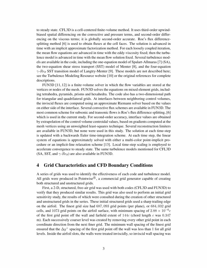
to steady state. CFL3D is a cell-centered finite-volume method. It uses third-order upwind-biased spatial differencing on the convective and pressure terms, and second-order differ-encing on the viscous terms; it is globally second-order accurate. Roe’s flux difference-splitting method [6] is used to obtain fluxes at the cell faces. The solution is advanced intime with an implicit approximate factorization method. For each loosely coupled iteration,the mean flow equations are advanced in time with the eddy-viscosity fixed; then the turbu-lence model is advanced in time with the mean flow solution fixed. Several turbulence mod-els are available in the code, including the one-equation model of Spalart-Allmaras [7] (SA),the two-equation shear stress transport (SST) model of Menter [8], and the four-equationγ-Reθ SST transition model of Langtry-Menter [9]. These models are not described here;see the Turbulence Modeling Resource website [10] or the original references for completedescriptions.

FUN3D [11, 12] is a finite-volume solver in which the flow variables are stored at thevertices or nodes of the mesh. FUN3D solves the equations on mixed element grids, includ-ing tetrahedra, pyramids, prisms and hexahedra. The code also has a two-dimensional pathfor triangular and quadrilateral grids. At interfaces between neighboring control volumes,the inviscid fluxes are computed using an approximate Riemann solver based on the valueson either side of the interface. Several convective flux schemes are available in FUN3D. Themost common scheme for subsonic and transonic flows is Roe’s flux difference splitting, [6]which is used in the current study. For second-order accuracy, interface values are obtainedby extrapolation of the control volume centroidal values, based on gradients computed at themesh vertices using an unweighted least-squares technique. Several reconstruction limitersare available in FUN3D, but none were used in this study. The solution at each time-stepis updated with a backwards Euler time-integration scheme. At each time step, the linearsystem of equations is approximately solved with either a multi-color point-implicit pro-cedure or an implicit-line relaxation scheme [13]. Local time-step scaling is employed toaccelerate convergence to steady state. The same turbulence models mentioned for CFL3D(SA, SST, and γ-Reθ) are also available in FUN3D.

4 Grid Characteristics and CFD Boundary Conditions

A series of grids was used to identify the effectiveness of each code and turbulence model.All grids were produced in Pointwise R©, a commercial grid generator capable of creatingboth structured and unstructured grids.

First, a 2-D, structured, free-air grid was used with both codes (CFL3D and FUN3D) toverify that they produced similar results. This grid was also used to perform an initial gridsensitivity study, the results of which were consulted during the creation of other structuredand unstructured grids in the series. These initial structured grids used a sharp trailing edgeon the airfoil. The finest grid size had 687, 093 grid points (per plane), or 684, 032 gridcells, and 1073 grid points on the airfoil surface, with minimum spacing of 2.88 × 10−6cof the first grid point off the wall and farfield extent of 144c (chord length c was 0.347m). Each successively coarser level was created by removing every other grid point in eachcoordinate direction from the next finer grid. The minimum wall spacing of the finest gridensured that the ∆y+ spacing of the first grid point off the wall was less than 1 for all gridlevels. Inside the airfoil slots, the walls were treated inviscidly, so inviscid wall spacing was

3

used (approximately in the range of 0.0001c − 0.001c). A view of the structured free-airgrid is shown in figure 2(a) and (b). Adiabatic no slip boundary conditions were appliedon the airfoil, except within the slots, whose side walls were treated as slip surfaces. Whenblowing was used, density and velocity were specified at the lower wall of the slot’s plenum,while pressure was extracted from the interior of the domain (density was set to freestream,and velocity was set in an iterative fashion to achieve the correct average velocity near theslot exit). When blowing was not used, the lower wall of the slot’s plenum was treated asa slip surface. At the outer boundary of the grid, a farfield Riemann-invariant boundarycondition was employed.

A series of 2-D structured grids incorporating inviscid upper and lower tunnel wallswas then created to identify the effect that the walls’ presence had on the lift coefficient andpressure distribution along the airfoil. A different grid was created for each angle of attackinvestigated (see, for example, figure 2(c)). These grids also used a sharp trailing edgeon the airfoil. The grid used here was based on the finest grid level from the free-air gridconvergence study. Its size was 407, 523 grid points (per plane), with 1073 grid points onthe airfoil surface and minimum spacing of 2.88× 10−6c of the first grid point off the wall.The tunnel walls extended from 5.76c in front of the airfoil quarter chord to 5.76c behind it.Normal grid spacing at the tunnel walls (treated inviscidly) was approximately in the rangeof 0.01c − 0.06c. Inside the airfoil slots, the walls were again treated inviscidly. For thesegrids, the boundary conditions on the airfoil surface and within its slots were the same asbefore. The upper and lower tunnel walls were treated as slip surfaces. At tunnel inflow, thetotal pressure and total temperature were specified according to adiabatic relations usingM = 0.03265: pt/pref = 1.00075, Tt/Tref = 1.00021, and Riemann invariants wereextrapolated from the interior of the domain. At tunnel outflow, static pressure was specifiedas p/pref = 1.0, and all other quantities were extrapolated from the interior.

A series of 2-D unstructured grids (with triangular elements) incorporating inviscidupper and lower tunnel walls was also created. A different grid was created for each angleof attack investigated (see, for example, figure 2(d)). To explore the influence of airfoiltrailing edge shape, these grids also used a blunt trailing edge on the airfoil, approximatelycorresponding to the actual bluntness of the wind tunnel model (about 0.0035c thickness).Although details are not provided in this report, the influence of the modeled trailing edgethickness was found to be insignificant in terms of the results of interest (surface pressurecoefficients and lift coefficients) for this study. These grids contained 384, 732 grid points(in the 2-D plane), and used 2141 grid points on the airfoil surface and minimum spacing of2.88× 10−6c of the first grid point off the wall. Tunnel wall extent was somewhat differentfrom the structured tunnel grids, with the downstream end extending to 8.64c. Normalgrid spacing at the tunnel walls (treated inviscidly) was approximately 0.007c. Boundaryconditions for these grids were the same as for the structured tunnel grids, except that theside walls inside the airfoil slots were treated viscously (the grids had finer spacing andthe boundary conditions were adiabatic no-slip). This viscous slot treatment was done toovercome a problem running FUN3D with some of the turbulence models.

A few runs were also performed in 3-D. For these, the 2-D, structured, tunnel grid wasextruded in the spanwise (y) direction a distance of y = 0.305 m, representing the tunnelhalf width. Grids spacing was clustered near y = 0, representing the tunnel side wall. Seefigure 2(e).

The grids used in this study each included the contracting portion of the blowing slots

4

between the slot plenums and the actual slot exit, as shown in figure 2(b). Therefore, theboundary condition at the plenum exit was set as a subsonic inflow when the slot wasblowing. The inflow velocity at this boundary was adjusted so that the jet velocity Uj(velocity at the slot exit line) matched the correct value for the chosen case. The target jetvelocities were found by rewriting Eq. (1) as

Uj =

√(1/2)CµcU2

∞h

(2)

then solving Eq. (2) for Uj using each value of Cµ included in the study. The target jetvelocity is equal to 32.693 m/s when Cµ = 5%, and 11.325 m/s when Cµ = 0.6%. Whennondimensionalized with the reference speed of sound, these two velocities are 0.096155and 0.03331, respectively.

To ensure that the jet velocity matched the target velocities for each value of Cµ, aniterative process was used in which the average velocity of the CFD solution across the slotexit line was found, then adjustments were made to the plenum inflow boundary conditionuntil the desired average jet velocity was attained (see figure 3). The inflow boundarycondition required was approximately the same regardless of whether the interior slot wallswere treated inviscidly or viscously.

5 Results

The results include grid sensitivity studies (both grid density as well as comparison of re-sults with structured and unstructured grids). Comparisons are made using different codesand different turbulence models. Efforts to model or capture transitional effects are de-scribed, and the effects of including the tunnel upper and lower walls are documented.Most computations are 2-D, but several 3-D trials were also explored (i.e., including tunnelside walls).

5.1 Structured Grid Sensitivity Studies

A grid sensitivity study was performed on the 2-D, structured, free-air grid. The original“fine” grid (684, 032 cells) was coarsened by removing every other grid point to produce a“medium” grid (171, 008 cells), then coarsened again to produce a “coarse” grid (42, 752cells). For the purposes of the grid sensitivity study, the case was run at several angles ofattack without blowing. Lift coefficient results are plotted in figure 4. The results indicatedlittle influence of grid density on lift coefficients over the angle of attack range of interest,so the medium grid was selected for use in obtaining further “free-air” results.

Notice in figure 4 that the experiment yielded an unusual lift curve shape. Rather thanan approximately linear progression of lift with angle of attack over the lower angles, theexperimental results exhibited a nonlinear increase in lift between approximately 5 and 10degrees. This is believed to be due to the presence of a laminar bubble near the airfoil’supper surface leading edge, which causes additional flow acceleration around it. As will bedescribed further below, the CFD was not able to capture this effect.

5

5.2 Code Comparison

Several test cases were run in both CFL3D and FUN3D to identify whether the two codeswould produce similar results for this case. The angles of attack used were 0, 5, 8, 10, and12 degrees. A sample of these results can be found in figure 5. These results show thaton the same sufficiently refined grid for this case, CFL3D and FUN3D produce practicallyidentical solutions.

5.3 Turbulence Model Comparison

Next, three turbulence models were examined using the same test cases. The results of theseruns can be found in figures 6 and 7. The SA and SST models displayed similar behaviorof relatively linear lift curve slope (failing to predict the nonlinear change in the lift curveslope between 5 and 10 degrees angle of attack). However, their pressure distributions werereasonable and consistent with each other and with the experiment.

The γ-Reθ turbulence model was used to attempt to capture the nonlinear lift curvebehavior. CL results at α = 5◦ appeared to be promising. The model yielded delay oftransition to turbulence on the upper surface, resulting in a series of small recirculating re-gions on the upper surface, which were products of a very large region of separated laminarflow. Example plots showing the extent of these regions can be seen in figure 7(b), (d), and(f). However, the experiment showed that laminar separation bubble reattachment occurredprior to 0.07 m along the chord in all cases for which the forward inactive slot on the up-per surface tripped the flow to turbulent [2]. Such large separated regions from the γ-Reθmodel indicated its failure to capture the tripping effect of this slot.

The cause of the failure of the γ-Reθ model has not been determined, but one poten-tial cause is the natural decay of freestream turbulence intensity inherent in the model.Turbulence intensity was specified to be 0.05%, based on information provided by the ex-perimenters. A large portion of that intensity might have decayed over the length of thegrid, so that the level near the airfoil was too low for the model to accurately predict tran-sition. Future efforts should focus on either adjusting the freestream turbulent boundaryconditions or disallowing their decay; also, time-accurate computations may be requiredwith this model to find the average of any inherent unsteadiness due to laminar separation.However, this model was not pursued further in the current study.

5.4 Forced Transition Study

To investigate the effects that transition location might have on the flow solutions, severaltest cases were run in which the transition location was specified in conjunction with theSA model. The ultimate goal of these particular runs was to determine if transition locationcould alter the solution enough to produce the behavior in the lift curve slope similar tothat seen in the experimental data. Transition effects were one of the first suspected causesof the behavior, since CFD is generally unreliable at predicting transition characteristics atlow Reynolds numbers such as the one in this problem. Seven transition locations on theupper surface of the airfoil were tested, ranging from approximately 5% (the location of theblowing slot) to 25% of chord length. Results from these tests can be found in figures 8and 9.

6

There were only small changes in the lift curve as the transition location varied (figure8). Looking at the solutions in more detail, as the laminar region increased in size, a smallregion of lower pressure was observed in the solution on the upper surface (the growing“hump” in the pressure distributions in figures 9(a) and (b)). Additionally, the flow solu-tion developed regions of recirculation if the transition was delayed far enough. See, forexample, figure 9(d), in which the skin friction goes negative for transition locations aftof approximately x/c = 0.07. However, these CFD trends do not appear to be matchingthe experimental data very well. Also, even though the lift coefficients increased slightlyas transition location was moved aft, the CL values from CFD never approached the levelsseen in the experimental data between 5◦ < α < 10◦.

This particular 2-D test failed to identify the cause of the nonlinearity in the experimen-tal lift curve. Therefore, the remainder of the CFD cases were run fully turbulent. Attemptsto capture the nonlinearity were abandoned in order to focus on the larger effects of theblowing slot on the lift curve.

5.5 Two-Dimensional Structured Grid Results

The first results to display the effects of slot blowing can be found in figure 10. These resultswere obtained from FUN3D runs on the 2-D, structured, free-air grid. The lift coefficientresults clearly exhibit the same trends as the experimental data, and are fairly accurate atlower angles of attack. However, the CFD failed to capture details such as the reduced stallangle of attack in the Cµ = 0.6% case.

The pressure distributions in figure 11 also match fairly well with the experimental datafor most cases. The main difference between CFD and experiment is that CFD tends topredict higher pressure on the upper surface than is found in the experiment. For casesin which massive separation is present in the flow, such as in figure 11(c), the pressuredistributions do not match well at all. This was expected, since RANS CFD generally failsto model massively separated flows correctly.

5.6 Structured Free-Air vs. Tunnel Grid Computations

New grids were created to examine the effect that upper and lower tunnel walls have on theflow solution. First, a structured tunnel grid was created (more details on grid constructionare found in Section 4). The results from this grid are compared to those from the free-airgrid in figures 12 and 13. This comparison shows that including the tunnel walls greatlyimproved correlation between the CFD solutions and the experimental results. Both liftcoefficient results and surface pressures better match the experimental data. For this reason,upper and lower tunnel walls were determined to be a necessary inclusion in all subsequentcomputations.

5.7 Two-Dimensional Unstructured Grid Results

Unfortunately, an undiagnosed issue within FUN3D caused the SST turbulence model tofail to produce a solution on the 2-D structured tunnel grid for all test cases. In an attempt toremedy this problem, an unstructured tunnel grid with viscous slot walls (but with otherwisesimilar characteristics as the 2-D structured tunnel grid) was created and tested. Both SA

7

and SST turbulence models produced useful results with this new grid. Overall, the effectsof slot blowing were captured very well in these CFD trials, as shown in figures 14 and15. At lower angles of attack, the changes in lift coefficient caused by the blowing werematched extremely well. At higher angles of attack, the CFD missed absolute levels butappeared to generally capture the trends with different blowing coefficients.

Unlike the results from the structured free-air grid shown in figure 10, these CFD trialscaptured the stall behavior of the airfoil for all three momentum coefficients: stall wasdelayed past the tested range of angles when Cµ = 5%, stall began around α = 15◦

when no slot blowing is used, and stall was induced early at around α = 9◦ when Cµ =0.6%. However, despite the fact that the start of stall behavior was correctly predicted, CFDperformance deteriorated beyond stall (massive separation). As expected for these cases,CFD typically did not converge to steady-state results. The error bars in figure 14 representthe amplitude with which the CFD solutions oscillated about the mean values at their mostconverged states. Because of this nonconvergence, time-accurate runs were required (asdescribed later). Comparisons of pressure coefficients (figure 15) were generally excellentfor both SA and SST, with the exception of the stalled high angle of attack case with Cµ =0.6%, shown in figure 15(f).

Figure 16 shows typical residual and lift histories for these cases, for FUN3D using theSA model. In the unstructured tunnel grid at α = 12.5◦, when Cµ = 5%, residuals weredriven to machine zero and lift was well converged. But when Cµ = 0 or 0.6%, the codedid not converge at this angle of attack: residuals were nonconvergent and the lift oscillated.

Prior to continuing with runs on the 2-D unstructured tunnel grids, a grid study analysiswas performed. FUN3D was run with the airfoil at α = 10◦ on several grid levels of boththe 2-D structured and unstructured tunnel grids. Lift coefficient results are plotted in figure17. In this plot, hg represents a measure of the average overall grid spacing. An infinitegrid is approached as hg → 0. From this plot, it is clear that the solutions on unstructuredtriangle grids are more grid-sensitive than solutions on the structured grid. For a givennumber of unknowns, the structured grid solution yields a result that is closer to the grid-converged result. However, both grid types approach approximately the same result, asexpected. Based on this result, the unstructured grid with hg ≈ 0.0015 appears to provideCL results that are within about 5% of the grid converged solution. This unstructured gridlevel was considered to be adequate for this study.

To further explore the nonconvergent (oscillating) solutions, all Cµ = 0.6% cases wererun again, time-accurately, in FUN3D. These cases had large amounts of separation at highangles of attack, so they were used to identify the effects of running time-accurately onthe CFD results. Results from the time-accurate trials, presented in figure 18 alongsidethe steady results, showed that the solution oscillations could be reduced dramatically withtime-accurate computations. Although the error bars, which represent the amplitude ofthe solution oscillation, were much smaller for the time-accurate solutions, generally theoverall trends in the lift behavior were similar to the steady-state runs. Although not shown,the Cp results for time-accurate runs were similar; i.e., still in reasonable agreement withexperiment except for stalled high angle of attack cases with Cµ = 0.6%.

Current results using FUN3D and the SST model are compared to independent SST re-sults using a different CFD code (Laufer [14]) in figure 19. The two codes used independently-generated grids, both including tunnel top and bottom walls. Laufer’s grids did not includeinternal plenums, but rather imposed blowing boundary conditions at the “slot exit” loca-

8

tion. Generally, the results from the two codes are in very close agreement. Note that, likeFUN3D, Laufer’s CFD results also missed the nonlinear behavior in the lift curve slopes,believed to be caused by the presence of a laminar bubble in the experiment.

Figure 20 shows the general effect of the blowing on the trailing edge separation loca-tion (in this case for FUN3D using the SA turbulence model). For no blowing, the airfoil atzero degrees angle of attack has no trailing edge separation, but separation appears as theangle of attack is increased. For example, at α = 10◦, separation occurs at approximatelyx/c = 0.72. With weak blowing at Cµ = 0.6%, the trailing edge separation is more pro-nounced (at α = 10◦, separation occurs ar approximately x/c = 0.51). On the other hand,strong blowing at Cµ = 5.0% has a Coanda effect and delays the presence of any trailingedge separation until beyond α = 10◦. Even as high as α = 15◦, separation is still near thetrailing edge (x/c = 0.86).

A comparison of experimental (PIV) and CFD velocity fields can be found in figure21, for α = 15◦. Detailed flow features could not be quantitatively matched, but as can beseen from the size of the recirculating regions, the CFD flow solutions were qualitativelycapturing the trends. Running time-accurately did not substantially improve the RANSresults.

5.8 Preliminary Three-Dimensional Computations

A limited number of 3-D trials were conducted to identify whether 3-D effects could havehad a significant impact on the experimental pressure data. The grid for these trials wasoriginally intended to be the 2-D unstructured grid, extruded approximately 80 times in thespanwise direction. However, 3-D runs in FUN3D failed to produce reasonable results onthis grid (due to a bug that was discovered, diagnosed, and fixed well after the current studywas completed).

For this reason, the structured 2-D grid was selected instead as the basis for the 3-Dgrid. This 2-D grid was extruded 81 times in the spanwise direction The spanwise spacingnear one side of the grid had viscous spacing (representing the wind tunnel side wall), whilethe other side had coarser spacing (representing the center of the wing section). This gridwas used in both CFL3D and FUN3D.

Visualizations of the 3-D effects when the wing is at α = 12.5◦ can be found in figure22. Here, in all blowing cases, corner effects create a large area of recirculation on theupper surface of the airfoil. At α = 12.5◦, CFL3D results with no blowing in figure 22(a)shows significant trailing edge separation across the entire wing span, along with a largecorner separation region near the side wall. With Cµ = 5% blowing (figure 22(b)), most ofthe wing is attached, but there is still a significant region of corner separation. Finally, withCµ = 0.6% (figure 22(c)), the entire wing is massively separated, and isolating the effectsof trailing edge separation and corner separation is difficult.

It is known that linear turbulence models can sometimes overpredict the size or influ-ence of corner separation [15, 16]. One known fix for this is the Quadratic ConstitutiveRelation (QCR2000) of Spalart [17]. In FUN3D, 3-D cases at a low angle of attack ofα = 5◦ were run with the SA model as well as with the SA-RC-QCR2000 model (where“RC” indicates an additional Rotation-Curvature correction [18]). Results are shown in fig-ure 23. For this case, the corner separation was relatively small, and the inclusion of RCand QCR2000 made little perceptible difference.

9

To investigate how much these 3-D effects have an impact on the pressure distributionalong the center of the wing section, which is where the pressure taps were located duringthe experiment, the pressure distributions along the wing centerline were plotted in figure24 for the same α = 5◦ case. From this zoomed-in plot, CFL3D and FUN3D are seen toproduce similar 3-D results (as well as similar 2-D results), with the 2-D and 3-D resultsshowing some difference from each other. The 2-D results yielded somewhat lower Cplevels on both the lower and upper surfaces, and tended to agree better with the experimentaldata than the 3-D computations. This plot indicates that even small 3-D effects in thesolution near the wall have some influence on the “two-dimensional” region near the tunnelcenter plane. This same conclusion was reached in an earlier study on a high-lift airfoil. [19]Simply stated, there is really no such thing as a “two-dimensional” experiment: any three-dimensionality present near side walls will affect to some degree the region of the flow thatis presumed to be nominally two dimensional.

Another interesting preliminary result from the 3-D trials can be seen in figure 25, whichplots FUN3D results at α = 12.5◦ (using the SA-RC-QCR2000 model on the structured3-D grid, no blowing). Figure 25(a) shows surface streamlines and surface pressure coef-ficient contours, indicating the three-dimensional nature of this solution. Nonetheless, theCp cuts along the span (shown in figure 25(b)) are relatively uniform, ranging from near thewall located at y = 0 m to the center plane located at y = 0.305 m. All cuts consistentlyunderpredict the negative peak Cp near the nose. However, the pressure distribution im-mediately aft of the blowing slot clearly changes across the span of the wing section. Thisindicates that a separated region exists behind the slot near the tunnel center plane, but notnear the wall. The effect appears to mimic the experimental data (taken along the tunnelcenterplane). 2-D CFD solutions for this case (not shown) did not indicate separated flowbehind the slot. This 3-D solution again illustrates the highly three-dimensional nature ofthis experiment, calling into question the use of 2-D CFD to try to compute this flow, foranything other than qualitative analysis.

6 Conclusions

RANS computations of an NACA 0018 airfoil (with and without leading edge blowing)were investigated. The independent codes CFL3D and FUN3D were confirmed to yieldvery close results when run on the same structured grid. Of the three turbulence mod-els tested, only the SA and SST models produced useful results in this study. These twomodels, run fully turbulent, predicted qualitative flow characteristics consistent with thosepresent in the experimental data for most test cases, although neither was able to predictthe nonlinear behavior of the experimental lift curve (believed to be caused by transitionaleffects). SA and SST were also fairly consistent with each other on all test cases. SAgenerally predicted slightly higher values of CL than SST, and the pressure and skin fric-tion distributions showed little difference. The γ-Reθ transition model predicted laminarregions that were too large, and therefore failed to produce reasonable results. However,it may yet prove to be applicable to this blowing slot problem if adjustments are made toits freestream boundary conditions. A forced transition study was also attempted, but itcould not predict the nonlinear behavior of the experimental lift curve. With the failure ofγ-Reθ and forced transition, attempts at predicting transitional effects within this flow were

10

abandoned. These failures indicate that RANS CFD in the production codes used here isnot well suited to predict transition characteristics for this type of flow.

Next, the effects of the upper and lower wind tunnel walls on the flow were examined.By comparing results from a free-air grid to results from structured tunnel grids, the tun-nel walls in this experiment were determinrd to have a significant impact on the pressuredistribution on the airfoil. To compare CFD results directly with the experimental data, theinclusion of upper and lower tunnel walls in computations is recommended.

Finally, the ability of 2-D RANS CFD to model the effects of slot blowing on the flowwas evaluated. Results from this study indicate that CFD is capable of qualitatively cap-turing the blowing effects reasonably well. Lift coefficient and pressure distribution resultsfrom CFD matched fairly well with experimental values at low angles of attack (α < 5◦,approximately). The lift curve nonlinear behavior was never captured, and CL values main-tained a mostly linear relationship with angle of attack up until the stall angle for each valueof Cµ. Overall, the predicted stall angle for each Cµ was well in line with each stall anglein the experiment.

As expected, 2-D RANS struggled to accurately model the test cases involving highlyseparated flows. Flow solutions for these cases were poor, even when run time accurately.Stalled solutions obtained with time-accurate RANS runs appeared to be more sensitive tothe choice of turbulence model, but neither model predicted surface pressure coefficientswell in comparison with experiment. Generally, 2-D RANS is not advisable for use on testcases in which the airfoil has stalled and in which the flow exhibits massive separation.

Preliminary 3-D computations suggested the presence of noteworthy three-dimensionaleffects present in this experiment, particularly at high angles of attack, suggesting that 2-DCFD should generally be avoided for all but qualitative trend analysis. Several interestingflow features were identified. More 3-D CFD trials are necessary to better understand thefull impact of these features on both the CFD and the experimental pressure data.

Overall, this experimental data set is a very challenging one for CFD. Many of itsfeatures—including transitional flow, low-aspect-ratio with three-dimensionality, and un-steady, massive separation—make 2-D steady RANS very unsuitable for its prediction, ina quantitative sense. Although the current mostly 2-D study (as well as another indepen-dent 2-D study referenced) was able to qualitatively capture the effects of different blowingrates on the lift, clearly the CFD results are quantitatively inaccurate, especially at higherangles of attack when significant separation is present. Future work should include moreattempts with transition prediction models, as well as 3-D simulations with eddy-resolving(i.e., beyond RANS) capability. Also, the qualitative ability of RANS to capture trends forother data from this experiment should be assessed, including unsteady pitching, unsteadylow frequency slot blowing, the combination of pitching and steady slot blowing, and thecombination of pitching and surging with unsteady slot blowing.

References

1. Greenblatt, D., “Unsteady Low-Speed Wind Tunnels,” AIAA Journal, Vol. 54, No. 6,2016, pp. 1817–1830.

11

2. Muller-Vahl, H. F., Strangfeld, C., Nayeri, C. N., Paschereit, C. O., Greenblatt, D.,“Control of Thick Airfoil, Deep Dynamic Stall Using Steady Blowing,” AIAA Journal,Vol. 53, No. 2, 2015, pp. 277–295, doi: 10.2514/1.J053090.

3. Muller-Vahl, H. F., Nayeri, C. N., Paschereit, C. O., Greenblatt, D., “Dynamic StallControl via Adaptive Blowing,” Renewable Energy, Vol. 97, 2016, pp. 47–64.

4. Poisson-Quinton, P. and Lepage, L., “Boundary Layer and Flow Control: Its Principlesand Application,” Survey of French Research on the Control of Boundary Layer andCirculation, edited by Lachmann, G. V., Vol. 1, Pergamon, New York, 1961, pp. 21–73.

5. Krist, S. L., Biedron, R. T., and Rumsey, C. L., “CFL3D User’s Manual (Version 5.0),”NASA-TM-208444, June 1998.

6. Roe, P. L., “Approximate Riemann Solvers, Parameter Vectors, and DifferenceSchemes,” Journal of Computational Physics, Vol. 43, 1981, pp. 357–372.

7. Spalart, P. R. and Allmaras, S. R., “A One-Equation Turbulence Model for Aerody-namic Flows,” Recherche Aerospatiale, No. 1, 1994, pp. 5–21.

8. Menter, F. R., “Two-Equation Eddy-Viscosity Turbulence Models for Engineering Ap-plications,” AIAA Journal, Vol. 32, No. 8, 1994, pp. 1598–1605.

9. Langtry, R. B. and Menter, F. R., “Correlation-Based Transition Modeling for Un-structured Parallelized Computational Fluid Dynamics Codes,” AIAA Journal, Vol. 47,No. 12, 2009, pp. 2894–2906.

10. Rumsey, C. L., “Turbulence Modeling Resource,” https://turbmodels.larc.nasa.gov,cited 11/15/2016.

11. Anderson, W. K. and Bonhaus, D. L., “An Implicit Upwind Algorithm for ComputingTurbulent Flows on Unstructured Grids,” Computers and Fluids, Vol. 23, No. 1, 1994,pp. 1–22.

12. Anderson, W. K., Rausch, R. D., and Bonhaus, D. L., “Implicit/Multigrid Algorithmfor Incompressible Turbulent Flows on Unstructured Grids,” AIAA Paper 95–1740–CP,12th Computational Fluid Dynamics Conference, San Diego, CA, June, 1995.

13. Nielsen, E. J., Lu, J., Park, M. A., and Darmofal, D. L., “An Implicit, Exact DualAdjoint Solution Method for Turbulent Flows on Unstructured Grids,” Computers andFluids, Vol. 33, No. 9, 2004, pp. 1131–1155.

14. Laufer, M., “CFD Predictions of Load Control Using Steady Blowing on a ThickAirfoil,” Proceedings of 34th Israeli Conference of Mechanical Engineering, Haifa,November 2016.

15. Yamamoto, K., Tanaka, K., and Murayama, M., “Comparison Study of Drag Predictionfor the 4th CFD Drag Prediction Workshop Using Structured and Unstructured MeshMethods,” AIAA Paper 2010-4222, June 2010.

12

16. Bordji, M., Gand, F., Deck, S., and Brunet, V., “Investigation of a Nonlinear Reynolds-Averaged Navier-Stokes Closure for Corner Flows,” AIAA Journal, Vol. 54, No. 2,2016, pp. 386–398.

17. Spalart, P. R., “Strategies for Turbulence Modelling and Simulations,” InternationalJournal of Heat and Fluid Flow, Vol. 21, 2000, pp. 252–263.

18. Shur, M. L., Strelets, M. K., Travin, A. K., and Spalart, P. R., “Turbulence Modeling inRotating and Curved Channels: Assessing the Spalart-Shur Correction,” AIAA Journal,Vol. 38, No. 5, 2000, pp. 784–792.

19. Rumsey, C. L., Lee-Rausch, E. M., Watson, R. D., “Three-Dimensional Effects inMulti-Element High Lift Computations,” Computers & Fluids, Vol. 32, 2003, pp. 631–657.

13

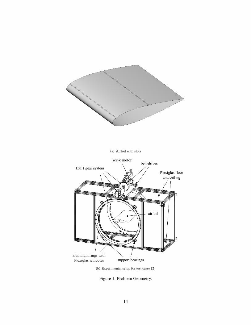
(a) Airfoil with slots

(b) Experimental setup for test cases [2]

Figure 1. Problem Geometry.

14

(a) 2-D, structured, free-air grid (b) 2-D, structured, free-air grid (close view)

(c) 2-D, structured, tunnel grid (d) 2-D, unstructured, tunnel grid

(e) 3-D, structured, tunnel grid

Figure 2. Examples of grids employed.

15

(a) Slot geometry (b) Example slot velocity profile

Figure 3. Jet velocity was considered to be the average velocity magnitude across the slotexit line (velocity is nondimensionalized by aref ).

Figure 4. Grid sensitivity study for 2-D, structured, free-air grids, no blowing, FUN3D withSA model.

16

(a) α = 0◦ (b) α = 0◦

(c) α = 5◦ (d) α = 5◦

(e) α = 10◦ (f) α = 10◦

Figure 5. Results from comparison cases between CFL3D and FUN3D, 2-D, structured,free-air grids, no blowing, with SA model.

17

Figure 6. Comparison of lift coefficient results from the three different turbulence models,2-D, structured, free-air grids, no blowing, CFL3D.

18

(a) α = 0◦ (b) α = 0◦

(c) α = 5◦ (d) α = 5◦

(e) α = 10◦ (f) α = 10◦

Figure 7. Comparison of pressure and skin friction coefficient results from the three turbu-lence models, 2-D, structured, free-air grids, no blowing, CFL3D.

19

Figure 8. Lift coefficient results from the forced transition study, 2-D, structured, free-airgrids, no blowing, CFL3D with SA model.

20

(a) α = 5◦ (b) α = 5◦

(c) α = 8◦ (d) α = 8◦

Figure 9. Pressure and skin friction coefficient results from the forced transition study, 2-D,structured, free-air grids, no blowing, CFL3D with SA model.

21

Figure 10. Lift coefficient results with slot blowing on a 2-D, structured, free-air grid,FUN3D with SA model.

22

(a) α = 5◦, Cµ = 0.6% (b) α = 5◦, Cµ = 5.0%

(c) α = 10◦, Cµ = 0.6% (d) α = 10◦, Cµ = 5.0%

Figure 11. Pressure distribution results with slot blowing on a 2-D, structured, free-air grid,FUN3D with SA model.

23

Figure 12. Comparison between lift coefficient results from a 2-D structured free-air gridand a 2-D structured tunnel grid, no blowing, FUN3D with SA model.

(a) α = 5◦ (b) α = 10◦

Figure 13. Comparison between pressure distribution results from a 2-D structured free-airgrid and a 2-D structured tunnel grid, no blowing, FUN3D with SA model.

24

Figure 14. Lift coefficient results with slot blowing on a 2-D unstructured tunnel grid,FUN3D (run in steady-state mode).

25

(a) α = 5◦, Cµ = 0% (b) α = 10◦, Cµ = 0%

(c) α = 5◦, Cµ = 5% (d) α = 10◦, Cµ = 5%

(e) α = 5◦, Cµ = .6% (f) α = 10◦, Cµ = .6%

Figure 15. Pressure distribution results with slot blowing on a 2-D unstructured tunnel grid,FUN3D (run in steady-state mode); error bars represent the amplitude of oscillation in thesolution.

26

(a) Density residual (b) Lift coefficient

Figure 16. Iterative convergence histories from FUN3D for α = 12.5◦ on a 2-D unstruc-tured tunnel grid, run in steady-state mode, SA model.

Figure 17. Grid convergence study using FUN3D on two different grid types; α = 10◦ intunnel, SA model.

27

Figure 18. Comparison of time-accurate and steady solutions for Cµ = 0.6% cases, 2-Dunstructured tunnel grid, FUN3D; error bars represent the amplitude of oscillation in thesolution.

28

Figure 19. Comparison of current 2-D FUN3D SST solutions with SST solutions fromSTARCCM+ in Laufer [14].

29

Figure 20. Effect of blowing on trailing edge separation location, 2-D unstructured tunnelgrid, FUN3D with SA model.

30

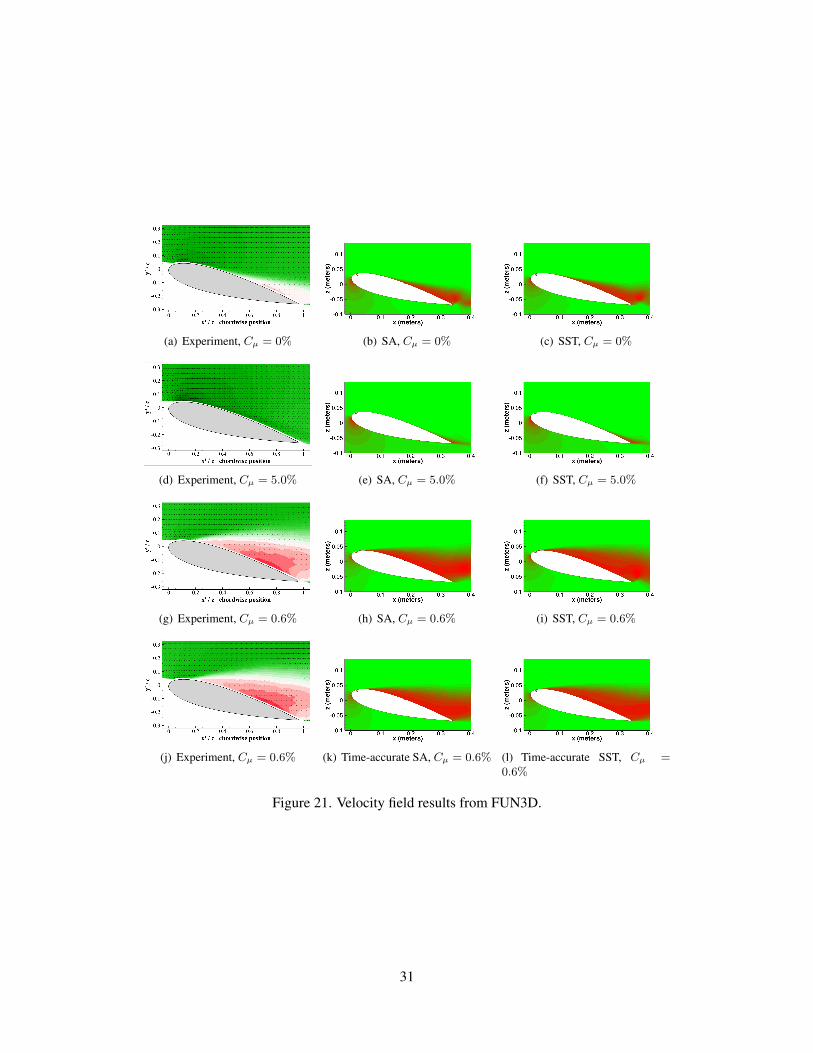
(a) Experiment, Cµ = 0% (b) SA, Cµ = 0% (c) SST, Cµ = 0%

(d) Experiment, Cµ = 5.0% (e) SA, Cµ = 5.0% (f) SST, Cµ = 5.0%

(g) Experiment, Cµ = 0.6% (h) SA, Cµ = 0.6% (i) SST, Cµ = 0.6%

(j) Experiment, Cµ = 0.6% (k) Time-accurate SA, Cµ = 0.6% (l) Time-accurate SST, Cµ =0.6%

Figure 21. Velocity field results from FUN3D.

31

(a) Cµ = 0% (b) Cµ = 5.0%

(c) Cµ = 0.6%

Figure 22. Initial 3-D results from CFL3D, displaying the effect that the juncture with thewind tunnel wall has on the overall flow; α = 12.5◦, 3-D structured grid with inviscidlower/upper walls, viscous side walls, SA model.

32

(a) SA model (b) SA-RC-QCR2000

Figure 23. Comparison of 3-D results from FUN3D with the SA turbulence modelwith and without Rotation/Curvature Correction (RC) and Quadratic Constitutive Relation(QCR2000); α = 5◦, Cµ = 0%, 3-D structured grid with inviscid lower/upper walls, vis-cous side walls.

Figure 24. Zoomed comparison of 3-D surface pressure coefficients from FUN3D andCFL3D to 2-D results (all with tunnel walls) and experimental values, α = 5◦.

33

(a) Surface streamlines (b) Surface pressure coefficients at cuts along the span

Figure 25. 3-D flow solution from FUN3D at α = 12.5◦, SA-RC-QCR2000.

34

REPORT DOCUMENTATION PAGE Form ApprovedOMB No. 0704–0188

The public reporting burden for this collection of information is estimated to average 1 hour per response, including the time for reviewing instructions, searching existing data sources,gathering and maintaining the data needed, and completing and reviewing the collection of information. Send comments regarding this burden estimate or any other aspect of this collectionof information, including suggestions for reducing this burden, to Department of Defense, Washington Headquarters Services, Directorate for Information Operations and Reports(0704-0188), 1215 Jefferson Davis Highway, Suite 1204, Arlington, VA 22202-4302. Respondents should be aware that notwithstanding any other provision of law, no person shall besubject to any penalty for failing to comply with a collection of information if it does not display a currently valid OMB control number.PLEASE DO NOT RETURN YOUR FORM TO THE ABOVE ADDRESS.

Standard Form 298 (Rev. 8/98)Prescribed by ANSI Std. Z39.18

1. REPORT DATE (DD-MM-YYYY)

01-04-20172. REPORT TYPETechnical Memorandum

3. DATES COVERED (From - To)

4. TITLE AND SUBTITLE

CFD Study of NACA 0018 Airfoil with Flow Control5a. CONTRACT NUMBER

5b. GRANT NUMBER

5c. PROGRAM ELEMENT NUMBER

5d. PROJECT NUMBER

5e. TASK NUMBER

5f. WORK UNIT NUMBER109492.02.07.01.01

6. AUTHOR(S)

Eggert, Christopher A.; Rumsey, Christopher L.

7. PERFORMING ORGANIZATION NAME(S) AND ADDRESS(ES)NASA Langley Research CenterHampton, Virginia 23681-2199

8. PERFORMING ORGANIZATIONREPORT NUMBER

L–20799

9. SPONSORING/MONITORING AGENCY NAME(S) AND ADDRESS(ES)National Aeronautics and Space AdministrationWashington, DC 20546-0001

10. SPONSOR/MONITOR’S ACRONYM(S)NASA

11. SPONSOR/MONITOR’S REPORTNUMBER(S)

NASA/TM–2017–219602

12. DISTRIBUTION/AVAILABILITY STATEMENT

Unclassified-UnlimitedSubject Category 02Availability: NASA STI Program (757) 864-9658

13. SUPPLEMENTARY NOTES

An electronic version can be found at http://ntrs.nasa.gov.

14. ABSTRACT

The abilities of two different Reynolds-Averaged Navier-Stokes codes to predict the effects of an active flow control device are evaluated.The flow control device consists of a blowing slot located on the upper surface of an NACA 0018 airfoil, near the leading edge. A secondblowing slot present on the airfoil near mid-chord is not evaluated here. Experimental results from a wind tunnel test show that a slot blowingwith high momentum coefficient will increase the lift of the airfoil (compared to no blowing) and delay flow separation. A slot with lowmomentum coefficient will decrease the lift and induce separation even at low angles of attack. Two codes, CFL3D and FUN3D, are used intwo-dimensional computations along with several different turbulence models. Two of these produced reasonable results for this flow, whenrun fully turbulent. A more advanced transition model failed to predict reasonable results, but warrants further study using different inputs.Including inviscid upper and lower tunnel walls in the simulations was found to be important in obtaining pressure distributions and liftcoefficients that best matched experimental data. A limited number of three-dimensional computations were also performed.

15. SUBJECT TERMS

CFD, flow control

16. SECURITY CLASSIFICATION OF:

a. REPORT

U

b. ABSTRACT

U

c. THIS PAGE

U

17. LIMITATION OFABSTRACT

UU

18. NUMBEROFPAGES

39

19a. NAME OF RESPONSIBLE PERSONSTI Information Desk (help@sti.nasa.gov)

19b. TELEPHONE NUMBER (Include area code)(757) 864-9658