ch 12- control charts for attributes p chart – fraction defective np chart – number defective c,...
TRANSCRIPT
Ch 12- Control Charts for Attributes
• p chart – fraction defective
• np chart – number defective
• c, u charts – number of defects
Defect vs. Defective
• ‘Defect’ – a single nonconforming quality characteristic.
• ‘Defective’ – items having one or more defects.
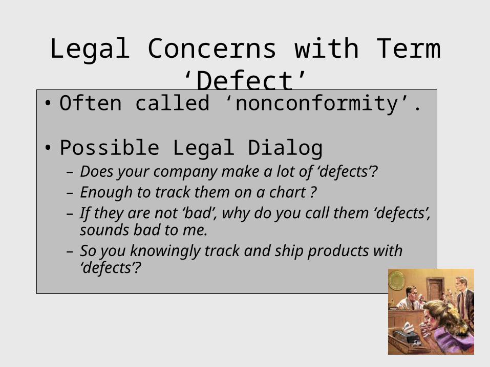
Legal Concerns with Term ‘Defect’• Often called ‘nonconformity’.
• Possible Legal Dialog– Does your company make a lot of ‘defects’?– Enough to track them on a chart ?– If they are not ‘bad’, why do you call them ‘defects’,
sounds bad to me.– So you knowingly track and ship products with
‘defects’?
Summary of Control Chart Types and LimitsTable 12.3
These are again ‘3 sigma’ control limits
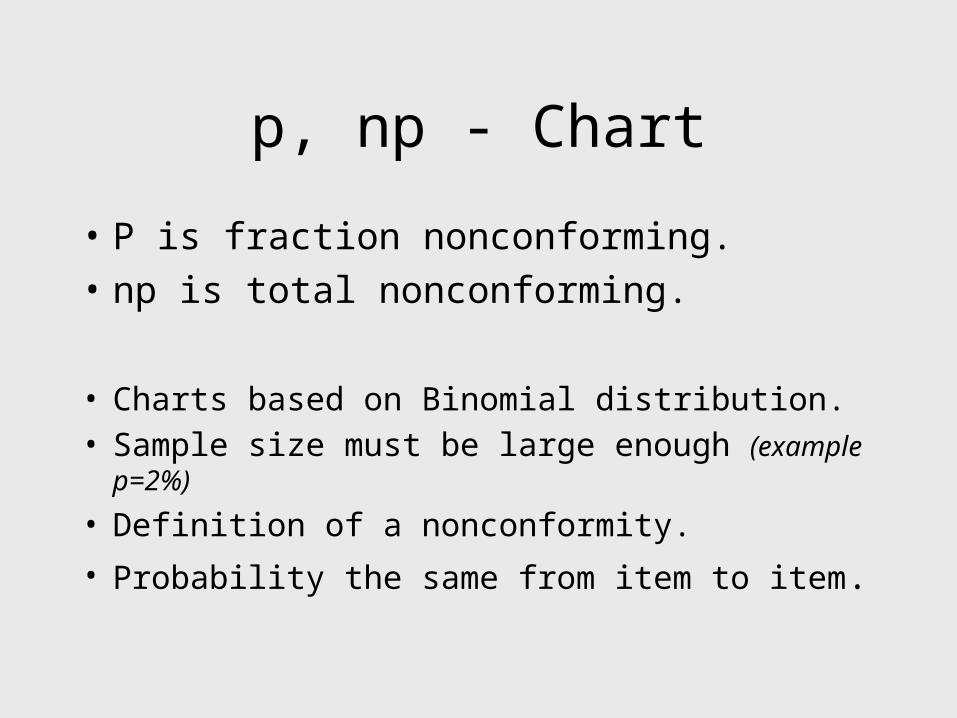
p, np - Chart
• P is fraction nonconforming.
• np is total nonconforming.
• Charts based on Binomial distribution.• Sample size must be large enough (example p=2%)
• Definition of a nonconformity.
• Probability the same from item to item.
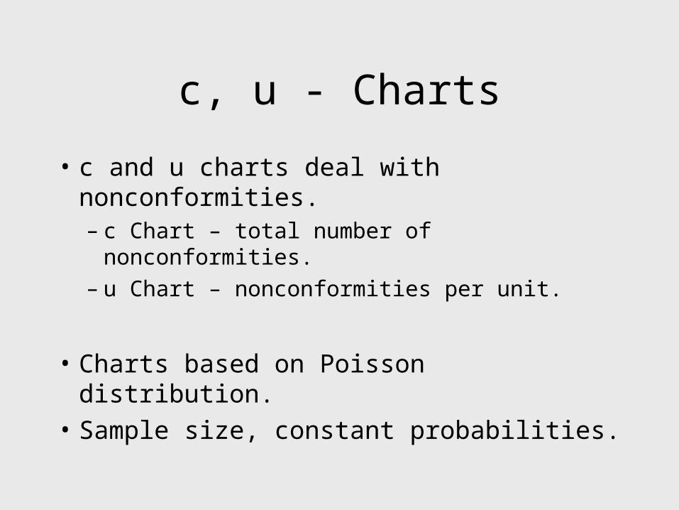
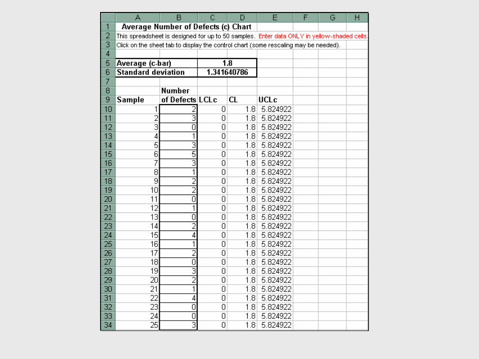
c, u - Charts
• c and u charts deal with nonconformities.– c Chart – total number of nonconformities.– u Chart – nonconformities per unit.
• Charts based on Poisson distribution.
• Sample size, constant probabilities.
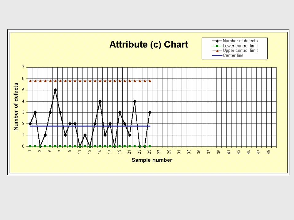
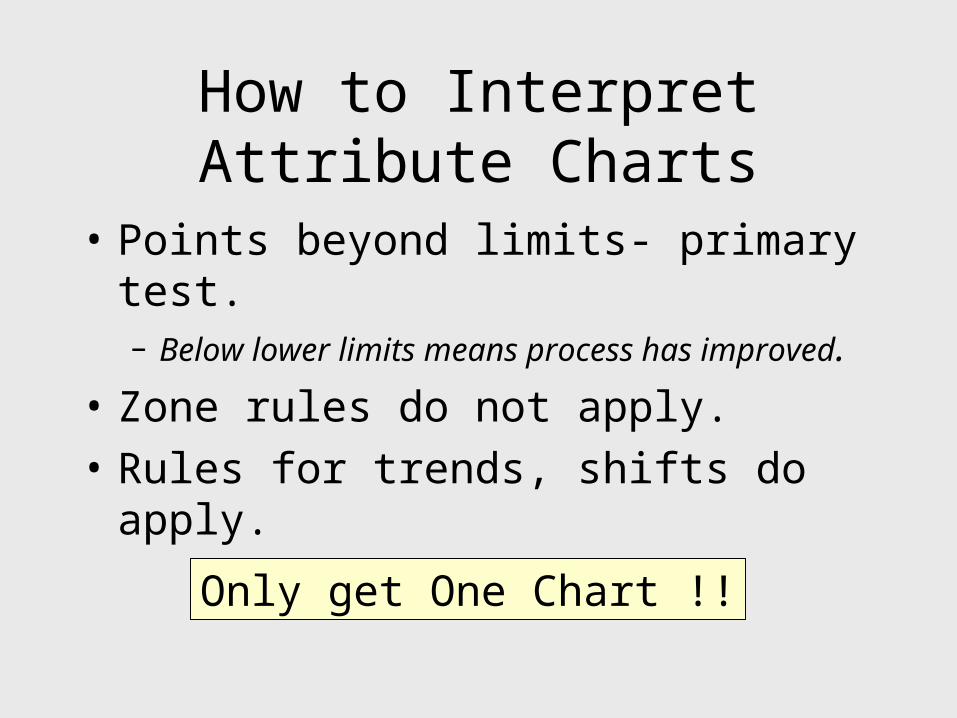
How to Interpret Attribute Charts
• Points beyond limits- primary test.– Below lower limits means process has improved.
• Zone rules do not apply.
• Rules for trends, shifts do apply.
Only get One Chart !!
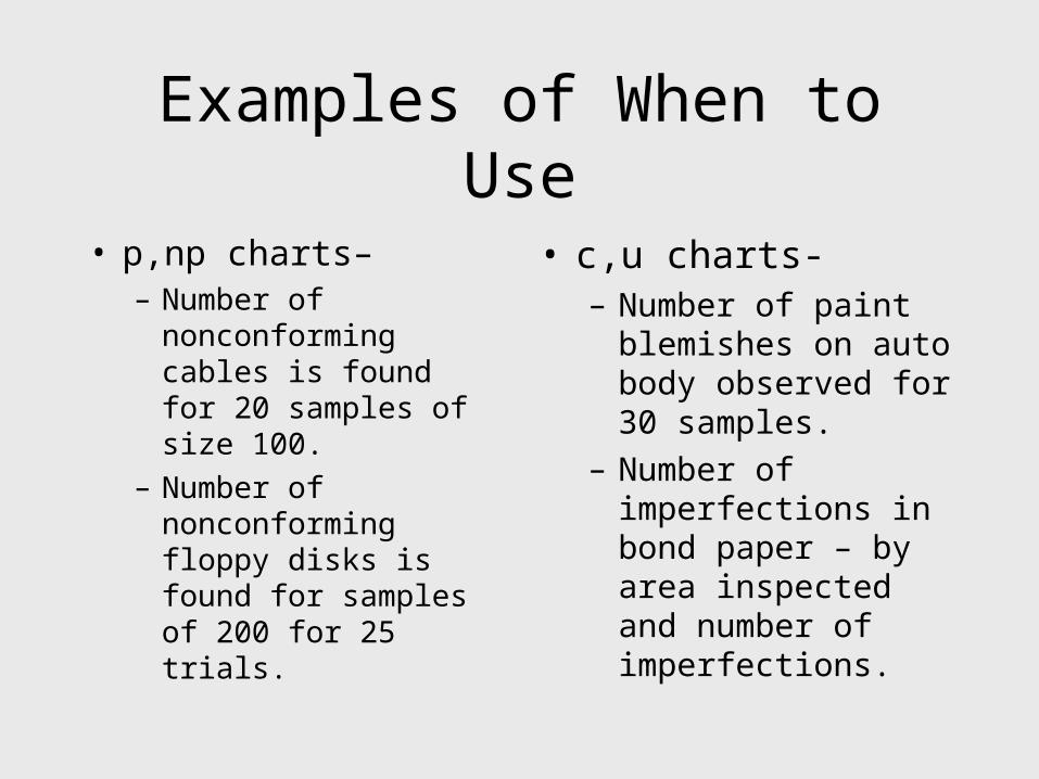
Examples of When to Use
• p,np charts–– Number of
nonconforming cables is found for 20 samples of size 100.
– Number of nonconforming floppy disks is found for samples of 200 for 25 trials.
• c,u charts-– Number of paint
blemishes on auto body observed for 30 samples.
– Number of imperfections in bond paper – by area inspected and number of imperfections.
13
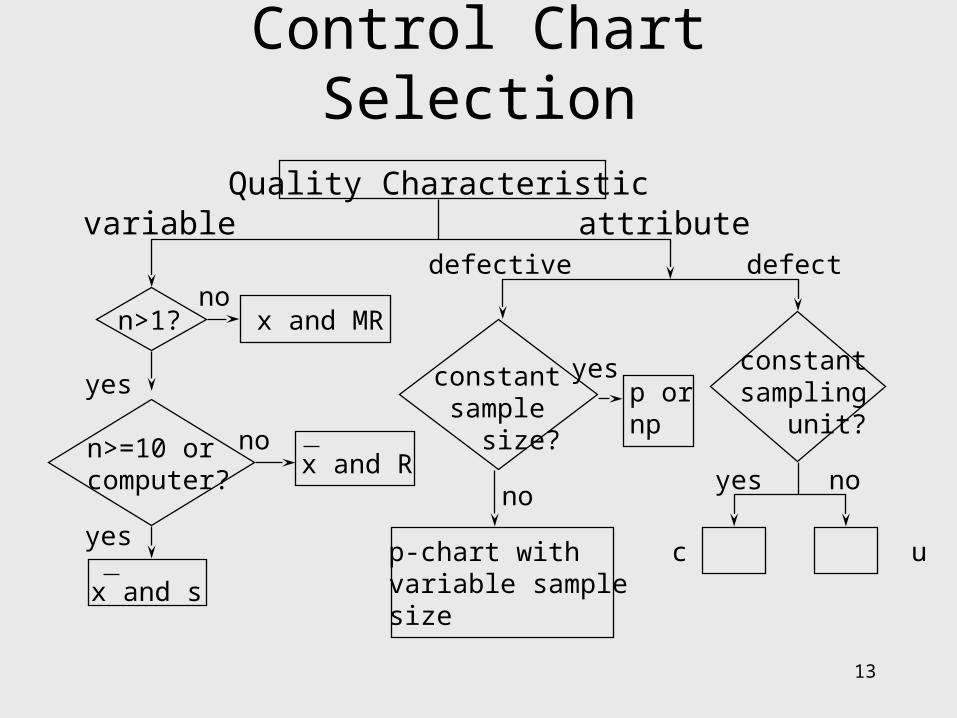
Control Chart SelectionQuality Characteristic
variable attribute
n>1?
n>=10 or computer?
x and MRno
yes
x and s
x and Rno
yes
defective defect
constant sample size?
p-chart withvariable samplesize
no
p ornp
yes constantsampling unit?
c u
yes no
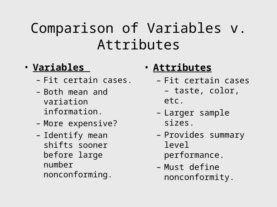
Comparison of Variables v. Attributes
• Variables – Fit certain cases.
– Both mean and variation information.
– More expensive?
– Identify mean shifts sooner before large number nonconforming.
• Attributes– Fit certain cases –
taste, color, etc.
– Larger sample sizes.
– Provides summary level performance.
– Must define nonconformity.
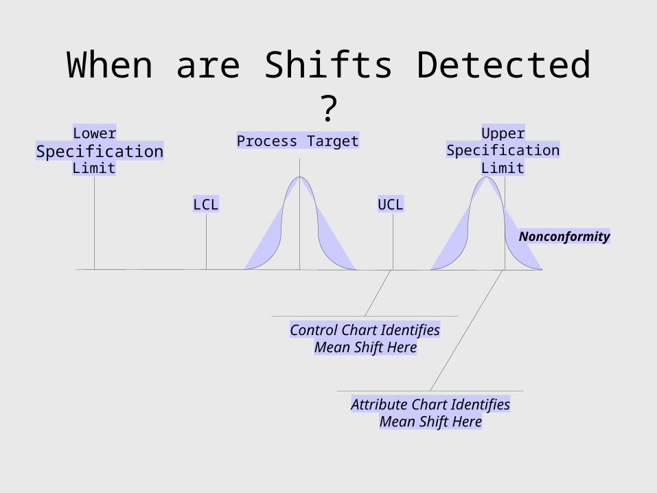
When are Shifts Detected ?Lower
SpecificationLimit
LCL UCL
UpperSpecification
Limit
Process Target
Nonconformity
Control Chart IdentifiesMean Shift Here
Attribute Chart IdentifiesMean Shift Here
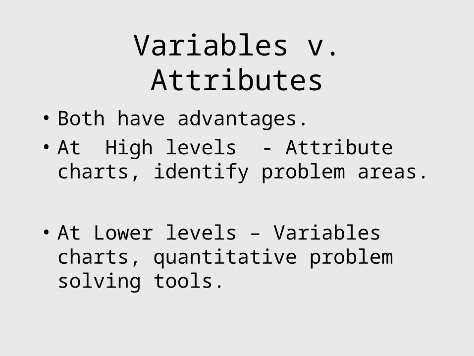
Variables v. Attributes
• Both have advantages.
• At High levels - Attribute charts, identify problem areas.
• At Lower levels – Variables charts, quantitative problem solving tools.

Intro to Acceptance Sampling
• Acceptance Sampling –
a historically significant topic but less used today.
• Part of Ch. 11 on Inspection Methods.
• Still used in some applications today.
History and Status
• Used extensively in WW II.
• Many Mil-Spec plans developed (105-E, ANSI/ASQC Z1.4-1993).
• Still popular as a defense procurement tool.– Very large lots, screening tool.– Low bid suppliers – no history.
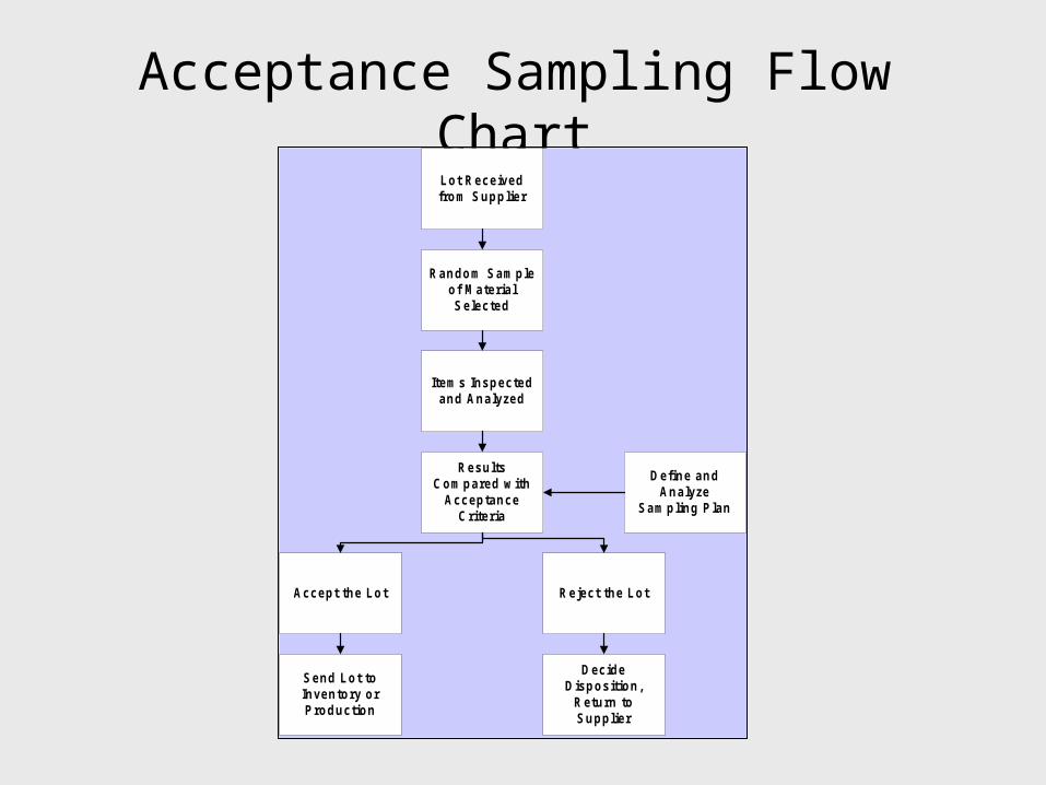
Acceptance Sampling Flow ChartLot Receivedfrom Supplier
Random Sampleof MaterialSelected
Items Inspectedand Analyzed
ResultsCompared w ith
AcceptanceCriteria
Define andAnalyze
Sampling Plan
Accept the Lot Reject the Lot
Send Lot toInventory orProduction
DecideDisposition,
Return toSupplier

Role of Producer and Consumer
Producer Consumer
Risk is a ‘good’ lot will be rejected and sent back.
Risk is a ‘bad’ lotwill be accepted.
Take a SampleSize ‘n’,
Accept if ‘c’ or less.
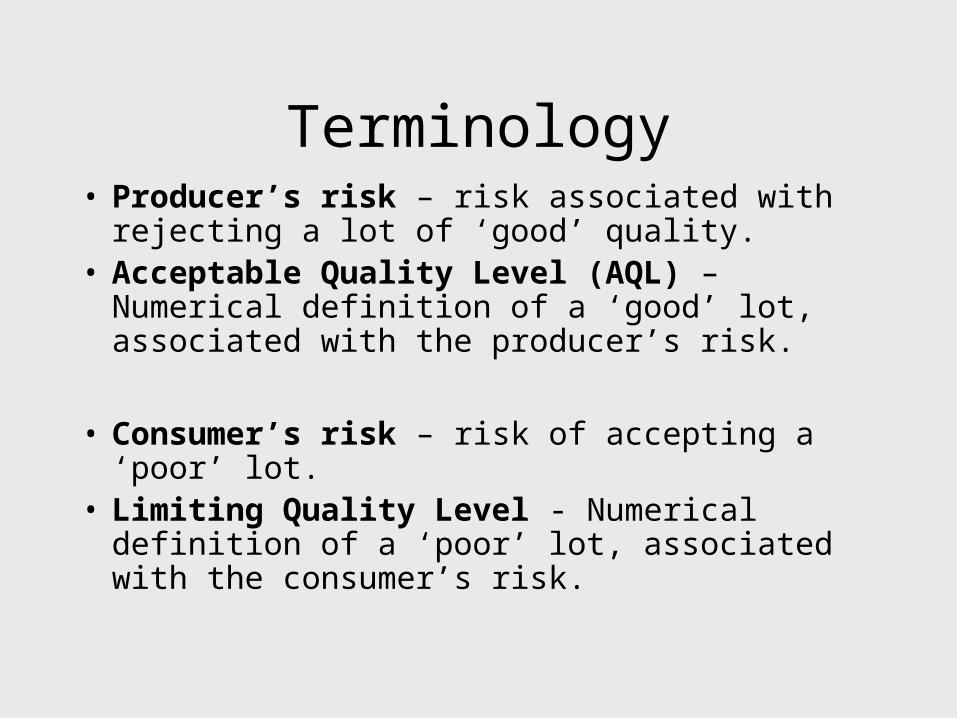
Terminology• Producer’s risk – risk associated with rejecting a
lot of ‘good’ quality.• Acceptable Quality Level (AQL) – Numerical
definition of a ‘good’ lot, associated with the producer’s risk.
• Consumer’s risk – risk of accepting a ‘poor’ lot.• Limiting Quality Level - Numerical definition of
a ‘poor’ lot, associated with the consumer’s risk.
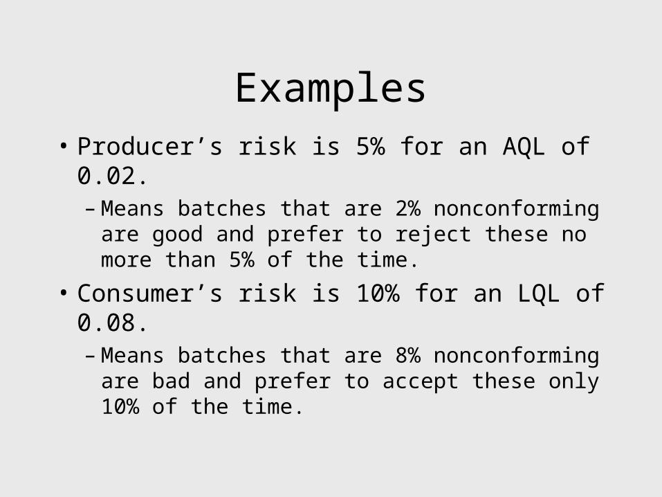
Examples
• Producer’s risk is 5% for an AQL of 0.02.– Means batches that are 2% nonconforming are
good and prefer to reject these no more than 5% of the time.
• Consumer’s risk is 10% for an LQL of 0.08.– Means batches that are 8% nonconforming are
bad and prefer to accept these only 10% of the time.
Operating Characteristic (OC) Curve
• Defines the performance of a sampling plan.
• Plots – probability of acceptance versus – proportion nonconforming (p).
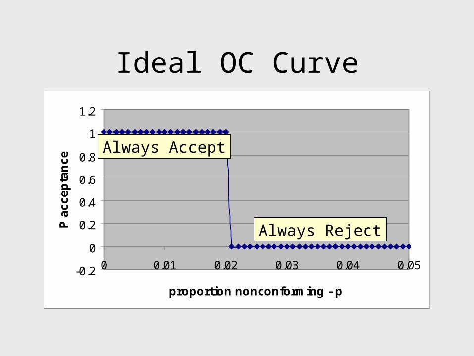
Ideal OC Curve
-0.2
0
0.2
0.4
0.6
0.8
1
1.2
0 0.01 0.02 0.03 0.04 0.05
proportion nonconforming - p
P a
cc
ep
tan
ce Always Accept
Always Reject
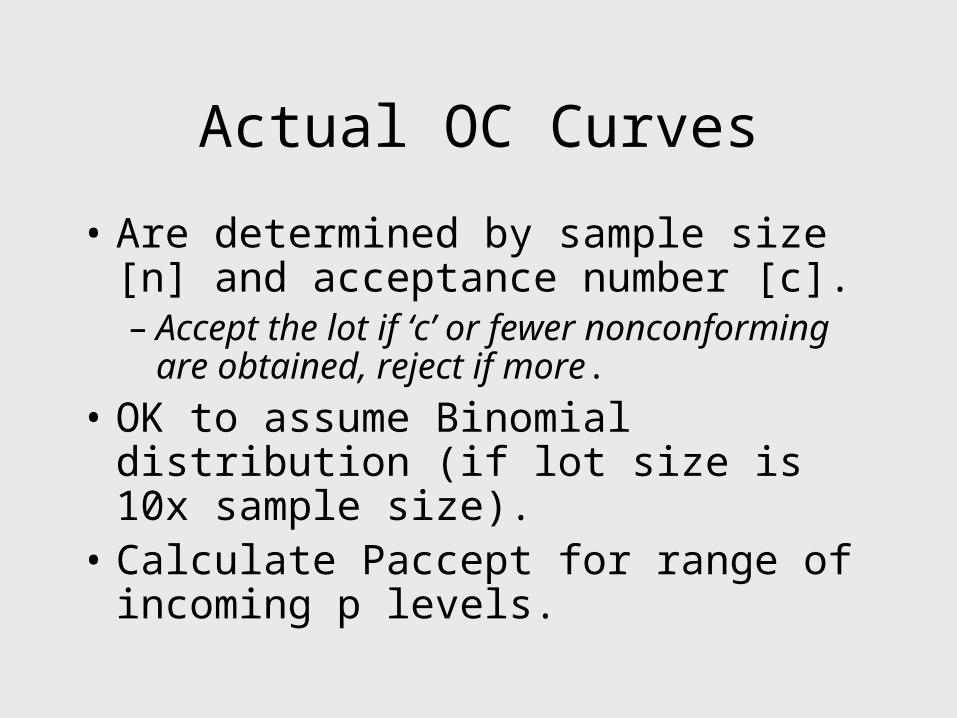
Actual OC Curves
• Are determined by sample size [n] and acceptance number [c].– Accept the lot if ‘c’ or fewer nonconforming are
obtained, reject if more.
• OK to assume Binomial distribution (if lot size is 10x sample size).
• Calculate Paccept for range of incoming p levels.
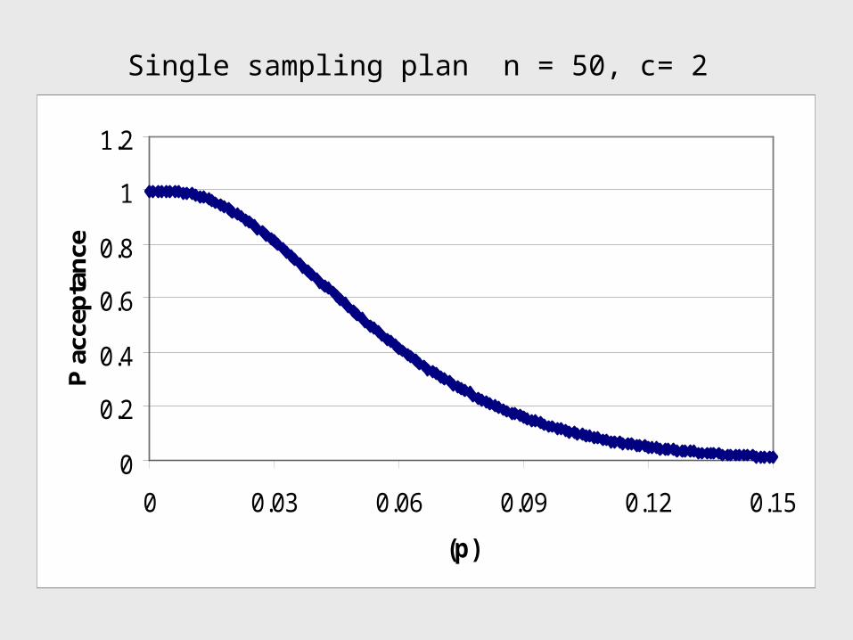
Sample problem
• Given a lot size of N=2000, a sample size n=50, and an acceptance number c=2.
• Calculate the OC curve for this plan.
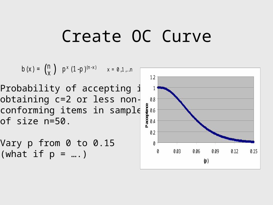
Create OC Curve
b(x) = p x (1-p) (n-x) x = 0,1,..nnx )(
Probability of accepting isobtaining c=2 or less non-conforming items in samples of size n=50.
Vary p from 0 to 0.15(what if p = ….)
0
0.2
0.4
0.6
0.8
1
1.2
0 0.03 0.06 0.09 0.12 0.15
(p)
P ac
cept
ance
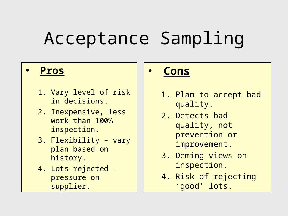
Acceptance Sampling
• Pros
1. Vary level of risk in decisions.
2. Inexpensive, less work than 100% inspection.
3. Flexibility – vary plan based on history.
4. Lots rejected – pressure on supplier.
• Cons
1. Plan to accept bad quality.
2. Detects bad quality, not prevention or improvement.
3. Deming views on inspection.
4. Risk of rejecting ‘good’ lots.
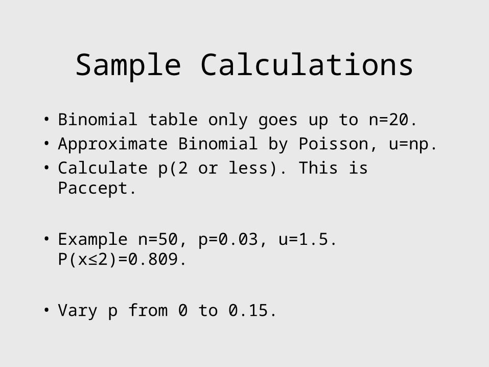
Sample Calculations
• Binomial table only goes up to n=20.• Approximate Binomial by Poisson, u=np.• Calculate p(2 or less). This is Paccept.
• Example n=50, p=0.03, u=1.5. P(x≤2)=0.809.
• Vary p from 0 to 0.15.
0
0.2
0.4
0.6
0.8
1
1.2
0 0.03 0.06 0.09 0.12 0.15
(p)
P a
ccep
tan
ceSingle sampling plan n = 50, c= 2
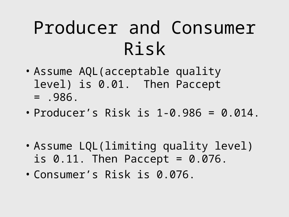
Producer and Consumer Risk
• Assume AQL(acceptable quality level) is 0.01. Then Paccept = .986.
• Producer’s Risk is 1-0.986 = 0.014.
• Assume LQL(limiting quality level) is 0.11. Then Paccept = 0.076.
• Consumer’s Risk is 0.076.
Designing Plan Performance
• Vary n and c to obtain different OC curves.
• Single and multiple sampling.
• Refer to standard published sampling plans.

Double Sampling Plan• Application of double sampling requires that a first sample of size n1
is taken at random from the (large) lot. The number of defectives is then counted and compared to the first sample's acceptance number a1 and rejection number r1. Denote the number of defectives in sample 1 by d1 and in sample 2 by d2, then: – If d1<= a1, the lot is accepted.
If d1 >= r1, the lot is rejected. If a1 < d1 < r1, a second sample is taken.
• If a second sample of size n2 is taken, the number of defectives, d2, is counted. The total number of defectives is D2 = d1 + d2. Now this is compared to the acceptance number a2 and the rejection number r2 of sample 2. In double sampling, r2 = a2 + 1 to ensure a decision on the sample. – If D2 <= a2, the lot is accepted.
If D2 >= r2, the lot is rejected.
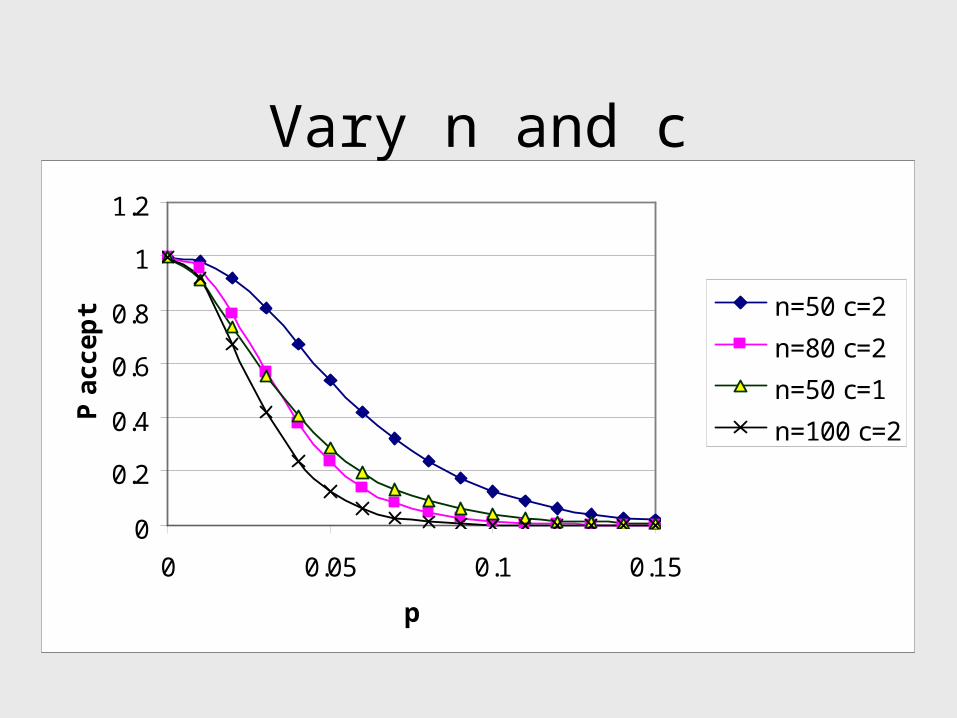
Vary n and c
0
0.2
0.4
0.6
0.8
1
1.2
0 0.05 0.1 0.15
p
P a
cc
ep
t n=50 c=2
n=80 c=2
n=50 c=1
n=100 c=2
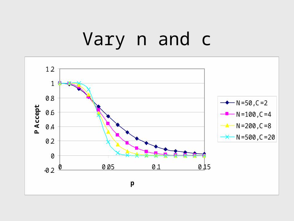
Vary n and c
-0.2
0
0.2
0.4
0.6
0.8
1
1.2
0 0.05 0.1 0.15
p
P A
ccep
t
N=50, C=2
N=100, C=4
N=200, C=8
N=500, C=20
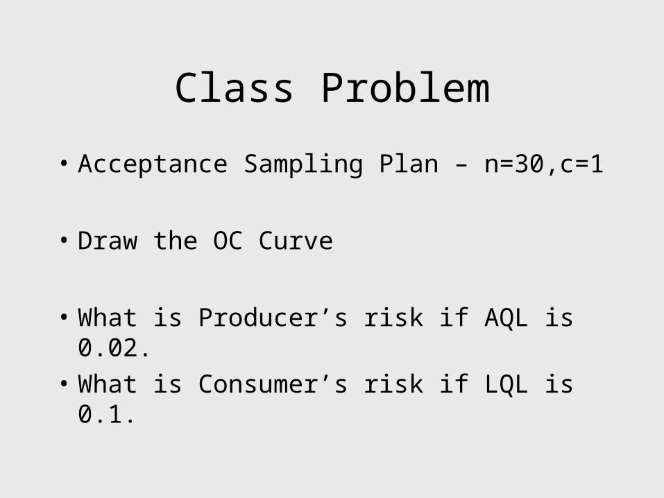
Class Problem
• Acceptance Sampling Plan – n=30,c=1
• Draw the OC Curve
• What is Producer’s risk if AQL is 0.02.
• What is Consumer’s risk if LQL is 0.1.
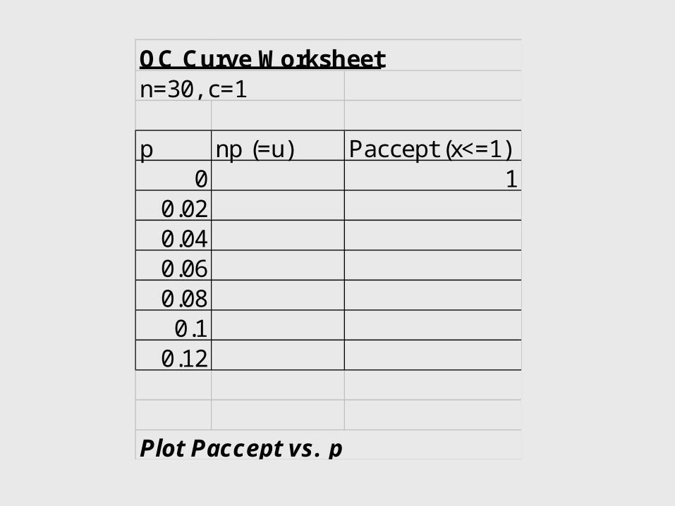
OC Curve Worksheetn=30, c=1
p np (=u) Paccept (x<=1)0 1
0.020.040.060.08
0.10.12
Plot Paccept vs. p

Homework
• Read Toyota Production System case and think about application of the Deming 14 points – we will discuss this next class.