Chalmers Publication Library

The flow around a simplified tractor-trailer model studied by large eddy simulation

This document has been downloaded from Chalmers Publication Library (CPL). It is the author´s

version of a work that was accepted for publication in:

Journal of Wind Engineering and Industrial Aerodynamics (ISSN: 0167-6105)

Citation for the published paper:Östh, J. ; Krajnovic, S. (2012) "The flow around a simplified tractor-trailer model studied bylarge eddy simulation". Journal of Wind Engineering and Industrial Aerodynamics, vol. 102pp. 36-47.

http://dx.doi.org/10.1016/j.jweia.2011.12.007

Downloaded from: http://publications.lib.chalmers.se/publication/154588

Notice: Changes introduced as a result of publishing processes such as copy-editing and

formatting may not be reflected in this document. For a definitive version of this work, please refer

to the published source. Please note that access to the published version might require a

subscription.

Chalmers Publication Library (CPL) offers the possibility of retrieving research publications produced at ChalmersUniversity of Technology. It covers all types of publications: articles, dissertations, licentiate theses, masters theses,conference papers, reports etc. Since 2006 it is the official tool for Chalmers official publication statistics. To ensure thatChalmers research results are disseminated as widely as possible, an Open Access Policy has been adopted.The CPL service is administrated and maintained by Chalmers Library.

(article starts on next page)

The Flow around a simplified tractor-trailer model studied by large

eddy simulation

Jan Osth∗, and Sinisa Krajnovic

Division of Fluid Dynamics,Department of Applied Mechanics,Chalmers University Of Technology,

SE-412 96 Goteborg, Swedenwww.tfd.chalmers.se/∼sinisa

Abstract

Large-eddy simulation (LES) is used to study the flow around a simplified tractor-trailermodel. The model consists of two boxes placed in tandem. The front box represents thecab of a tractor-trailer road vehicle and the rear box represents the trailer. The LES wasmade at the Reynolds number of 0.51 × 106 based on the height of the rear box and theinlet air velocity. Two variants of the model were studied, one where the leading edges onthe front box are sharp and one where the edges are rounded. One small and one large gapwidth between the two boxes were studied for both variants. Two computational grids wereused in the LES simulations and a comparison was made with available experimental forcemeasurements. The results of the LES simulations were used to analyze the flow field aroundthe cab and in the gap between the two boxes of the tractor-trailer model. Large vorticalstructures around the front box and in the gap were identified. The flow field analysis showedhow these large vortical structures are responsible for the difference in the drag force for themodel that arises when the leading edges on the front box are rounded and the gap widthis varied.

Keywords: Vehicle Aerodynamics, Large Eddy Simulation, Simplified Tractor-trailer, GapFlow, CFD, Bluff Body Aerodynamics, Tandem Configuration

1. Introduction

The aerodynamic performance of heavy vehicles is an area in which improvements canbe made even though there have been great achievements in the past half century. Theaerodynamic forces that act on a vehicle during driving affect the operation of the vehicle indifferent ways. The side and lift forces may cause instabilities and handling problems. Thedrag force affects the velocity and acceleration of the vehicle as well as the fuel consumption.For commercial vehicles, overcoming the drag requires a lesser part of the total fuel, that

∗Email address: ojan@chalmers.se (Jan Osth)

Preprint submitted to Journal of Wind Eng. Ind. Aerodyn. January 17, 2012

goes to overcome all the driving resistances (such as drag, rolling and climbing resistance)during cruising, when compared with a passenger car. The energy that can be saved forcommercial vehicles by decreasing the aerodynamic drag is still apparent.The pressure drag, which makes up the major part of the aerodynamic drag on a tractor-trailer unit, essentially comes from four parts of the vehicle: the forebody of the tractor,the rear part of the trailer, the underhood plus wheels and the gap between the tractor andthe trailer. The latter is a large contributor to drag. The shape of the tractor cab willinfluence what the flow conditions will be for the trailer. The contribution to the overalldrag coefficient of a tractor-trailer unit from the gap is influenced by the width of the gapbetween the tractor cab and trailer. The gap width will henceforth be denoted by g andexpressed in non-dimensional form g/b or sometimes g/

√A, where b and A are characteristic

length and area, respectively, of the specific model studied. In general, the smaller the gapis, the smaller will the positive contribution to the drag coefficient of the gap be. This is ofcourse also dependent on the relationship between the heights of the tractor and the trailer.The drag coefficient of simplified tractor-trailer units with a cab with rounded shape issmallest for zero gap widths and increases slightly with increasing gap width. Around a gapwidth of g/

√A ≈ 0.5 (A is the model cross-sectional area) a sudden increase in drag occurs

(McCallen et al. [2000], Allan [1981], Hammache and Browand [2002]). This increase in dragis completely due to an increase in the drag of the trailer alone. The drag of the tractor cabvaries very little with increasing gap widths (Allan [1981], Hammache and Browand [2002]).As noted above, the drag of the entire unit depends a great deal on the flow in the gap, andeven more so when the vehicle is operating in cross-wind environments. With an increasingyaw angle of the oncoming airflow, the drag for the unit is significantly increased and unitswith sharp-edged cabs are affected most (Hucho [1998], Barnard [1996]). One reason forthis is that the region of stagnation on the trailer increases when the air flow comes fromthe side. Various successful add-on devices for reducing the contribution to the overall dragfrom the gap are today standard practice among heavy vehicle manufacturers. These are,e.g., deflector plates mounted on the cab roof and cab side extenders that direct the air overthe trailer and fairings mounted on the trailer, which help flow attachment in the gap duringcross-wind conditions. Other devices such as gap seals have proven to be able to furtherreduce the drag but are not yet in common use. For a historical view of the development oftruck aerodynamics see Cooper [2002, 2003].Allan [1981] made aerodynamic measurements in the wind tunnel of Soupthampton on asimplified tractor-trailer model at Reynolds number Reb = 0.51 × 106 based on the heightof the trailer box, b. The model he used is also the one used in the present numerical study,see Fig. 1. The model consists of one front box representing the tractor cab and a rear boxrepresenting the trailer. The front box has a height, width and depth of 0.92 b, 0.92 b and0.67 b, respectively. The rear box has a height, width and depth of b, b and 2.5 b, respectively.The ground clearance of the front and rear box is 0.21 b and 0.5 b, respectively. This setupgives a realistic placement of the cab and trailer with respect to the standard shape ofEuropean tractor-trailer trucks at the time. Two variants of the model were investigatedby Allan [1981], one model with sharp leading edges on the front box and another withrounded edges. The width of the gap between the two boxes was varied and the drag was

2

measured for 0◦ yaw angle. The results are shown in Fig 2. It was found that the value ofthe drag coefficient of the model with sharp leading edges on the front box was more stablewith respect to increased gap width. The model with rounded edges exhibited significantlysmaller drag coefficient for small gap widths but the drag increased dramatically for largergap widths and even gave a larger drag coefficient than for the sharp model. This behaviorof the drag coefficient of another simplified tractor-trailer model with a rounded front wasalso found later in other experimental studies (Hammache and Browand [2002], Arcas et al.[2004]).

U∞

0.67b

0.92b

0.92b 0.21b0.5b

g/b

2.5b b

b

o

y

x

z

0.713b

Figure 1: Dimensions of the model used in the experiments by Allan [1981] and in the present LES simula-tions. The variant with sharp leading edges on the front box is shown.

3

0 0.2 0.4 0.6 0.8

0.7

0.8

0.9

1

1.1

1.2

1.3

1.4

Sharp model

Round model

DragCoeffi

cient

g/b

Figure 2: Experimental results for the drag coefficient for the two models investigated, redrawn from Allan[1981].

Large Eddy Simulations (LES) were used by Krajnovic et. al. for a number of differentbluff body flows, such as the flow around a generic train (Hemida et al. [2005]), a simplifiedbus (Krajnovic and Davidson [2003]), a finite tall cylinder (Krajnovic [2011]), and the groundvehicle Ahmed body reference model (Krajnovic and Davidson [2005a,b]). See Krajnovic[2009] for a further review of LES for bluff body flows. These studies have shown that LESprovides useful information about the flow structures around vehicle-shaped bluff bodies atmoderate Reynolds numbers and can correctly predict the global quantities, such as thedrag coefficient. In LES the large scale turbulent motions are resolved directly while theinfluence of the smaller scales on the large scales is modelled (Pope [2000]). It is a transientmethod that enables the study of the large scale unsteady structures that are characteristicof bluff body flows.

The aim of the work in this paper is to explain the underlying flow physics of the dis-parities in the behavior of the drag coefficients of the two models in the study by Allan[1981] (see Fig. 2). LES should be well suited to simulate the massively separated flowaround the simplified tractor-trailer model. This introductory part of the paper is followedby a section where the simplified tractor-trailer models used in the simulations are presented.Then follows a section that describes the numerical details used in the simulations which isfollowed by a section where results are presented and interpreted. In the last section thepaper is summarized.

2. Method

2.1. Description of the model

In the present work, LES simulations of the flow around the tractor-trailer model fromAllan [1981] are conducted. At a zero yaw angle, the flow physics will be explored aroundthe model with square leading edges on the front box and the model with rounded leadingedges on the front box. The general dimensions of the model are shown in Fig. 1. In theround model, both the horizontal and vertical leading edges on the front box are rounded

4

with the non-dimensional radius 0.08 b which is the same as in the experiments by Allan[1981]. This necessarily extends the length of the front box for the round model by 0.08 b.The two boxes are connected to each other with two cylinders of diameter 0.08 b, which areplaced horizontally in the gap at half of the height of the front box. The complete model wassuspended from the arms of an overhead balance in the experiments. No locations or detailsof these arms were reported, and the arms are therefore neglected in the present simulations.Two different gap widths are investigated for both models, one small gap width of g/b = 0.17(b = 0.305 m is the width of the rear box) and one large gap width of g/b = 0.67. Theexperimental results from Allan [1981] indicate that the sharp model has a drag coefficientof 1.02 and the round model 0.77 for g/b = 0.17, based on the cross-sectional area of therear box (b2 = 0.093m2). For g/b = 0.67, the sharp model has a drag coefficient of 1.09 andthe round model 1.28. The Reynolds number based on b and the free-stream velocity in theexperiments was Reb = 0.51× 106 and this is the same in the present simulations.

2.2. Numerical set-up

2.2.1. LES Governing Equations

The governing LES equations are the incompressible Navier-Stokes and the continuityequations filtered with the implicit spatial filter of characteristic width ∆:

∂ui

∂t+

∂

∂xj

(uiuj) = −1

ρ

∂p

∂xi

+ ν∂2ui

∂xj∂xj

− ∂τij∂xj

(1)

and∂ui

∂xi

= 0. (2)

Here, ui and pi are the resolved velocity and pressure, respectively, and the bar over thevariable denotes filtering.

The influence of the small scales of the turbulence on the large energy carrying scales inEq. (1) appears in the SGS stress tensor, τij = uiuj − uiuj. The algebraic eddy viscositymodel originally proposed by Smagorinsky [1963] is used in the present work for its simplicityand low computational cost. The Smagorinsky model represents the anisotropic part of theSGS stress tensor, τij, as:

τij −1

3δijτkk = −2νsgsSij (3)

where νsgs = (Csf∆)2|S| is the SGS viscosity and

Sij =1

2

(

∂ui

∂xj

+∂uj

∂xi

)

(4)

is the resolved rate-of-strain tensor and |S| =(

2SijSij

)1

2 . The value of the Smagorinskyconstant CS = 0.1 previously used for similar types of vehicle bluff body flows (Krajnovic[2009]) is used in the present work. f in the expression for the SGS viscosity is the vanDriest damping function

5

f = 1− exp(n+

25) (5)

where n+ is the wall normal distance in viscous units. The filter width, ∆, is definedin this work as ∆ = (∆1∆2∆3), where ∆i are the computational cell sizes in the threecoordinate directions.

2.2.2. Numerical method

Equations (1) and (2) are discretized using a commercial finite volume solver, AVL Firev2009.1 (AVL [2009]), for solving the incompressible Navier-Stokes equations using a collo-cated grid arrangement. The convective fluxes are approximated by a blend of 95% linearinterpolation of second order accuracy (central differencing scheme) and of 5% upwind dif-ferences of first order accuracy (upwind scheme). The diffusive terms containing viscous plussub-grid terms are approximated by a central differencing interpolation of second order ac-curacy. It should be noted that for complex geometries using non-equidistant computationalgrids a commutation error is introduced since the formulation of Eq. (1) assumes that thefiltering operation and spatial derivation commutes, which is not true on non-equidistantgrids. This error is of the same order as the truncation error of the second order linearinterpolation scheme (see e.g. Ghosal and Moin [1995]). The time marching procedure isdone using the implicit second-order accurate three-time level scheme

(

dφ

dt

)

n

=3φn − 4φn−1 + φn−2

2∆tn, ∆tn = t− tn−1 = tn−1 − tn−2 (6)

where indices ”n” and ”n-1” denote the new and old time levels, respectively. To deter-mine the pressure, the discrete form of the filtered continuity equation (Eq. 2) is convertedinto an equation for the pressure correction. The SIMPLE algorithm (Patankar and Spalding[1972]) is used to update the pressure and velocity fields so that they satisfy the continuityequation.

2.2.3. Computational grids

For all of the four cases, two different computational grids were used to check grid de-pendence of the results. The structured grids were made with the commercial grid generatorsoftware Ansys ICEM-CFD and consist of only hexahedral elements. The coarse grids con-sisted of 10.2, 10.3, 11.0 and 12.1 million cells for the square model with a small gap width(Case 1), the rounded model with a small gap width (Case 2), the square model with a largegap width (Case 3) and the rounded model with large gap width (Case 4), respectively. Ahorizontal cut in the grid for Case 2 is shown in Fig. 3. The finer grids consisted of 13.8,14.6, 16.3 and 17.1 for Case 1-4, respectively. The grids consist of rectangular blocks, andthe model enclosed in an O-grid. About 70% of all the cells are in the O-grid, which formsa belt with a width of 0.25 b around the front box and 0.4 b around the rear box.

6

Figure 3: A horizontal cut in the coarse computational grid for Case 2.

7

2.2.4. Boundary conditions

The computational domain is shown in Fig. 4. The size of the cross section correspondsto the wind tunnel used in the experiments by Allan [1981]. A uniform free-stream velocityof U∞ = 24.4 m/s is set at the inlet, which is the same as used in the wind tunnels tests. Novalue of the turbulence intensity of the free-stream velocity in the wind tunnel was reportedby Allan [1981]. Thus, the steady velocity profile was used at the inlet in the present work.On the floor, the moving ground used in the experiments is simulated by setting the velocitycomponent in the streamwise direction on the ground equal to U∞ together with the no-slipboundary condition. Since the velocity of the moving ground is equal to the free-streamvelocity, there is no boundary layer on the floor and it consequently doesn’t need to beresolved. The no-slip condition is used on the lateral walls and roof. However, the boundarylayers are not resolved here. On the tractor-trailer model the no-slip condition is used. Thehomogeneous Neumann boundary condition is applied at the outlet.

8

5.6b

6.9b

32.7b

8.0b

21.0b

Figure 4: The computational domain used in the present LES simulations. b = 0.305m.

2.2.5. Spatial and temporal resolution

For both the coarse and fine grids the wall normal resolution on the truck model is n+ < 1in all four cases. To achieve this, the size in normal direction of the first cell is 0.00016 b.The maximum values of n+ are found on the very edges of the square geometries. For thecoarse grids, the resolution in the streamwise direction is 2 < ∆s+ < 100 and 2 < ∆l+ < 30in the direction parallel to the surface of the body and normal to the streamwise direction,respectively. The fine grids have 2 < ∆s+ < 70 and 2 < ∆l+ < 20. Here, ∆n+ = n〈uτ 〉t/ν,∆s+ = ∆s〈uτ 〉t/ν, ∆l+ = ∆l〈uτ 〉t/ν and 〈uτ 〉t is the time-averaged friction velocity. Thetime step in the coarse grid simulations was 5·10−5 s and in the fine grid simulations 4·10−5 sgiving a CFL number below one in all of the simulations. All the cases were initially runfor a physical time of 1 second to let the flow develop. This corresponds to a fluid particletravelling the length of the entire numerical wind tunnel 2.5 times. Time averaging startedafter the initial developing period. The filtered variables were averaged over some convectivetime of t · U∞/L = 100, where L is the length of the model. This corresponds to a fluidparticle travelling approximately 11 times through the wind tunnel.

3. Results

The denotations that are used in this section for the different parts of the geometry areshown in Fig. 5. The base face of the rear box, denoted RB BF, is not seen in the figure.The four different cases, Cases 1 - 4 are listed in Table 1. ’Sharp model’ refers to the caseswith sharp leading edges on the front box and ’round model’ refers to the cases with roundedleading edges on the front box.

9

η

FB FF

FB TF

RB FF

FB BF

FB LFY-cut

Z-cut

FB GFz

y

x

Figure 5: Denotations of parts of the model used in the present work. Coordinate η is used to plot thepressure coefficient (CP ) and starts at origo and goes clockwise around the symmetry line on the front box.FB FF, FB TF, FB BF, FB LF, FB GF and RB FF denote the front face of the front box, the top face ofthe front box, the base face of the front box, the lateral face of the front box, the face closest to the groundand the front face of the rear box, respectively. Y-cut cuts the front box at half of its width (y = 0) and isthe symmetry plane. Z-cut cuts the front box at z = 0.46b.

Table 1: The four different cases studied in the present work.

Name Leading edge on Gap widthfront box

Case 1 Sharp g/b = 0.17Case 2 Round g/b = 0.17Case 3 Sharp g/b = 0.67Case 4 Round g/b = 0.67

10

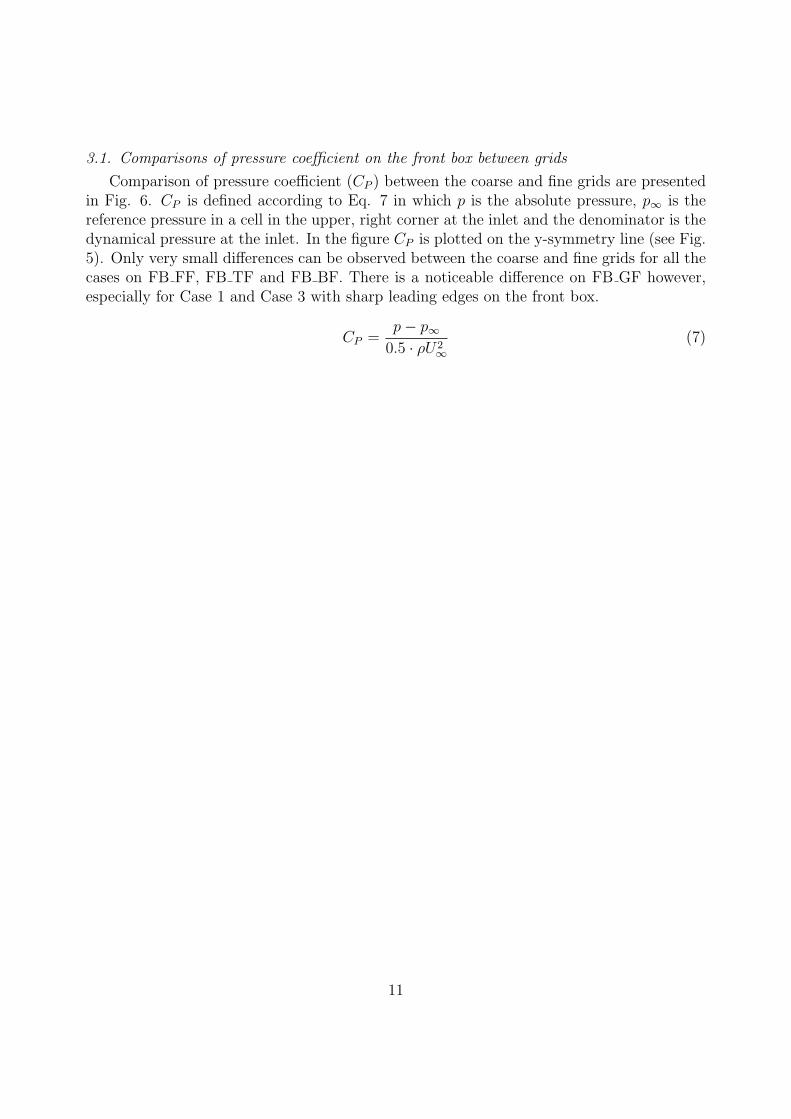
3.1. Comparisons of pressure coefficient on the front box between grids

Comparison of pressure coefficient (CP ) between the coarse and fine grids are presentedin Fig. 6. CP is defined according to Eq. 7 in which p is the absolute pressure, p∞ is thereference pressure in a cell in the upper, right corner at the inlet and the denominator is thedynamical pressure at the inlet. In the figure CP is plotted on the y-symmetry line (see Fig.5). Only very small differences can be observed between the coarse and fine grids for all thecases on FB FF, FB TF and FB BF. There is a noticeable difference on FB GF however,especially for Case 1 and Case 3 with sharp leading edges on the front box.

CP =p− p∞0.5 · ρU2

∞

(7)

11

a)0 0.2 0.4 0.6 0.8 1

−1

−0.8

−0.6

−0.4

−0.2

0

0.2

0.4

0.6

0.8

1

CP

η

FB FF FB TF FB BF FB GF

b)0 0.2 0.4 0.6 0.8 1

−1

−0.8

−0.6

−0.4

−0.2

0

0.2

0.4

0.6

0.8

1

CP

η

FB FF FB TF FB BF FB GF

c)0 0.2 0.4 0.6 0.8 1

−1

−0.8

−0.6

−0.4

−0.2

0

0.2

0.4

0.6

0.8

1

CP

η

FB FF FB TF FB BF FB GF

d)0 0.2 0.4 0.6 0.8 1

−1

−0.8

−0.6

−0.4

−0.2

0

0.2

0.4

0.6

0.8

1

CP

η

FB FF FB TF FB BF FB GF

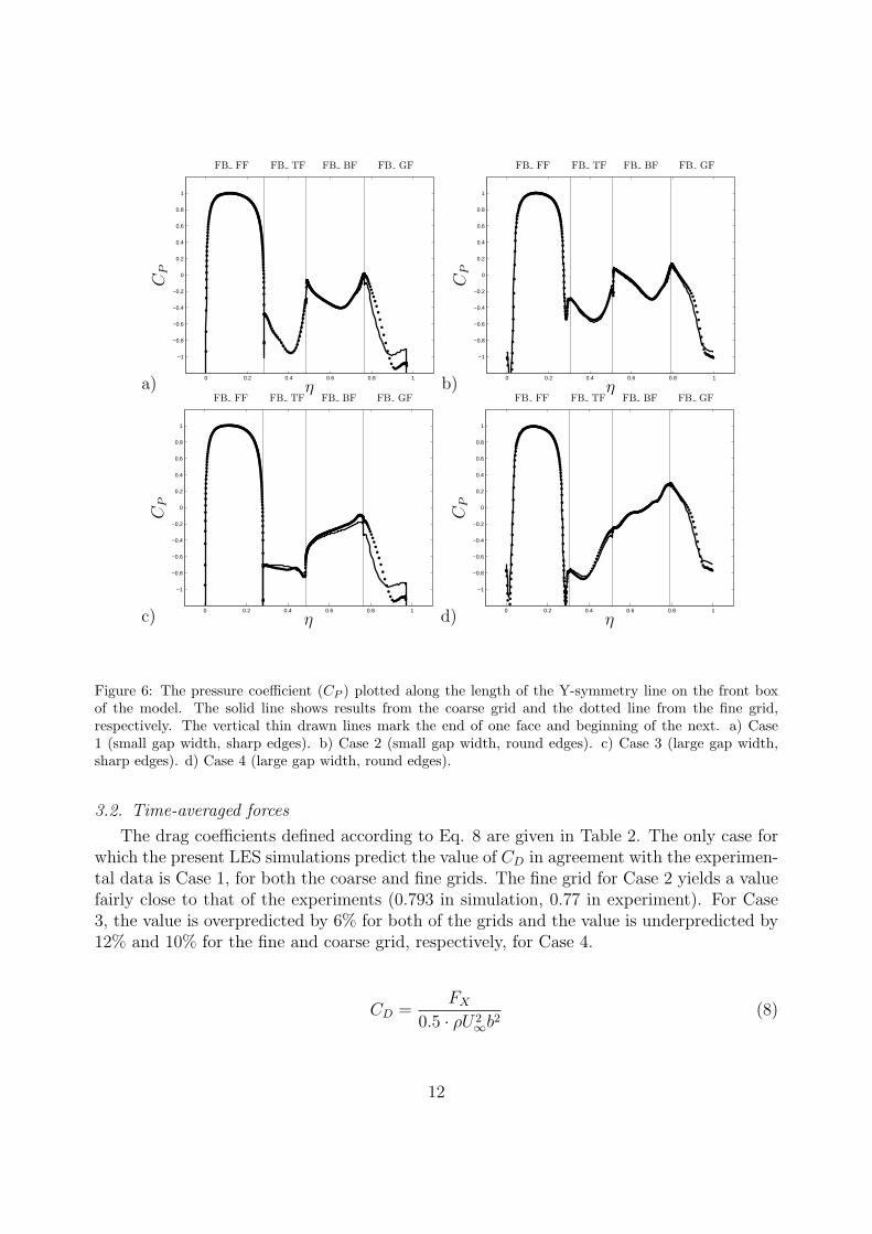
Figure 6: The pressure coefficient (CP ) plotted along the length of the Y-symmetry line on the front boxof the model. The solid line shows results from the coarse grid and the dotted line from the fine grid,respectively. The vertical thin drawn lines mark the end of one face and beginning of the next. a) Case1 (small gap width, sharp edges). b) Case 2 (small gap width, round edges). c) Case 3 (large gap width,sharp edges). d) Case 4 (large gap width, round edges).

3.2. Time-averaged forces

The drag coefficients defined according to Eq. 8 are given in Table 2. The only case forwhich the present LES simulations predict the value of CD in agreement with the experimen-tal data is Case 1, for both the coarse and fine grids. The fine grid for Case 2 yields a valuefairly close to that of the experiments (0.793 in simulation, 0.77 in experiment). For Case3, the value is overpredicted by 6% for both of the grids and the value is underpredicted by12% and 10% for the fine and coarse grid, respectively, for Case 4.

CD =FX

0.5 · ρU2∞b2

(8)

12

Table 2: Force coefficients results from the simulations together with the available experimentaldata from Allan [1981].|∆CD| is the difference between the computed and the experimental value.

Aerodynamic coefficients CD rms(CD) |∆CD|Case 1 exp 1.02 - -Case 1 fine 1.023 0.041 < 1%Case 1 coarse 1.022 0.039 < 1%

Case 2 exp 0.77 -Case 2 fine 0.793 0.056 3%Case 2 coarse 0.823 0.044 7%

Case 3 exp 1.09 - -Case 3 fine 1.160 0.084 6%Case 3 coarse 1.157 0.077 6%

Case 4 exp 1.28 - -Case 4 fine 1.124 0.041 12%Case 4 coarse 1.146 0.048 10%

The contributions to CD of the entire model from the four contributing faces are shownin Fig. 7. In Allan [1981] the contributions to CD from FB FF and RB BF are said to bealmost constant over different gap widths for both the sharp and round models. This is alsotrue in the present simulations, which can be seen in Figs. 7a,d. The changes in CD for theentire model when the gap width is varied are thus only due to changes in the contributionsfrom the two gap faces, FB BF and RB FF. Much can be understood about the differencebetween the models (sharp and round leading edges on the front box) by looking at thegraphs in Fig. 7. The rounding dramatically reduces CD on FB FF by some 55 % (see Fig.7a.) for both gap widths (as expected when rounding the front edge of a prismatic body,see Cooper [1985]). CD is however also reduced by some 50 % on the base face of the frontbox (FB BF) with round front edges on the front box for both gap widths (see in Fig. 7b).This was found in both the present numerical study and the experimental study by Allan[1981]. This is a result of the proximity of the rear box to the front box. The large gainin decreased drag for the entire model when the edges of the front box are rounded andthe gap width kept small is lost due to an increase in the contribution to the drag fromthe rear box for large gap widths. The flow mechanism behind this will be explained inSection 3.3 and 3.4. Figure 7c shows the contribution to CD from RB FF for the sharp andround models, respectively. On the sharp model, there is a negative contribution to CD fromRB FF in both the present simulations and experiments for both gap widths. For the roundmodel with a small gap width, there is a slightly positive contribution to CD from RB FF.The contribution to CD from RB FF increases a great deal as the gap width is increased tog/b = 0.67 for the round model. Thus, starting with Case 1 (g/b = 0.17 and sharp leadingedges), the decrease in CD that is gained by rounding the leading edges on the front boxis lost almost entirely due to the contribution to CD from the front face of the rear box(RB FF) when the gap width is increased.

13

a)

0 0.2 0.4 0.6 0.80

0.2

0.4

0.6

0.8

Sharp model (Coarse)

Sharp model (Fine)

Round model (Coarse)

Round model (Fine)

DragCoeffi

cient

g/b

FB FF

b)

0 0.2 0.4 0.6 0.80

0.1

0.2

0.3

0.4

0.5

Sharp model (Coarse)

Round model (Coarse)

Sharp model (Fine)

Round model (Fine)

Sharp model (Exp)

Round model (Exp)

DragCoeffi

cient

g/b

FB BF

c)0 0.2 0.4 0.6 0.8

−0.4

−0.2

0

0.2

0.4

0.6

0.8

DragCoeffi

cient

g/b

BF FF

d)0 0.2 0.4 0.6 0.8

0

0.1

0.2

0.3

0.4

0.5

DragCoeffi

cient

g/b

RB BF

Figure 7: Contribution to the drag coefficent of the entire model from the four different contributing faces.a) FB FF. b) FB BF c) RB FF. d) RB BF. Note that in a) and d) only results from the coarse and finegrid simulations are presented since there were no experimental results available for these faces.

14

3.3. Time-averaged flow structures

The time-averaged flow fields around the models are presented in this section and all theresults shown come from the fine grid simulations. The four cases (Cases 1-4) will be sub-divided into the groups ”small gap width” and ”large gap width” to emphasize the differencein the flow structures that emerges by rounding the leading edges of the front box.

3.3.1. Small gap width

This section presents the mean flow around the two cases (Case 1 and Case 2) with a smallgap width (g/b = 0.17). Case 1 has a sharp leading edge on the front box and Case 2 has arounded. Vortex cores are computed by the algorithm in the EnSight visualization package.The method for vortex core identification is based on critical-point concepts for fluid flow (e.gPerry and Chong [1987]) and finds eigenvalues and eigenvectors to the rate-of-deformationtensor of the filtered velocity, ∂ui/∂xj . A full description of the algorithm is given by Sujudiand Haimes [1995]. The algorithm can produce non-existing cores and should only be usedas a tool to help localize vortices (Sujudi and Haimes [1995]). Streamlines around cores areused in the present work to assure that the cores really exist. The vortical structures thatare of interest to us in this work are large vortical structures in the order of magnitude of bcaused by separation of the flow at leading and base edges. Streamlines of the time-averagedvelocity projected onto the surface are also used to reveal features in the flow. The streamlinepattern on the surface will reveal points where the streamline slope is indeterminate (i.e.all the spatial derivatives of the velocity are zero). These points are called critical points(Perry and Chong [1987]) and by interpreting the pattern of these points the salient featuresin the flow can be understood. Critical points and bifurcation lines are shown in Fig. 8.Three kinds of critical points can be formed: nodes, foci and saddles (see. Fig. 8). The firsttwo can be either stable or unstable. Other patterns that the streamlines form are negative(NBL) and positive (PBL) bifurcation lines. NBLs are associated with flow separation andPBLs are associated with flow attachment. For an example of how streamline patterns havebeen used previously in vehicle aerodynamics we refer to Krajnovic and Davidson [2005b].

15

UN SF SP

NBL PBL

Figure 8: Critical points and bifurcation lines. SP is a saddle point, SF is a stable focus, UN is an unstablenode, NBL is a negative bifurcation line and PBL is a positive bifurcation line.

16

a)

VSTF

VSLF

FB FF

FB TF

FB LF

RB FF

b)

VRTF

VRLF

VRLF1NBL

VRLF2

Figure 9: Streamlines of the time-averaged velocity projected onto the surface of the body (white lines)together with vortex cores (black drawn lines) and streamlines projected onto planes around vortex cores(black lines). a) Case 1 (small gap width, sharp edges). b) Case 2 (small gap width, round edges)

17

Time-averaged flow structures around the cab are presented for Case 1 in Fig. 9a andCase 2 in Fig. 9b. In the figures, the white lines are streamlines of the time-averaged velocityprojected onto the surface of the body. The black streamlines of the time-averaged velocityare projected onto planes around the vortex cores (solid black lines). For both cases, thefree-streaming air hits the front face of the front box (FB FF) and separates at the leadingedges. Over the top face of the front box (FB TF) the flow separations form vortices VSTF

(see Figs. 9a and 16a) and VRTF (see Figs. 9b and 16b) for Case 1 (sharp model) and Case2 (round model), respectively. Outside of the lateral face of the front box (FB LF) for Case1 the vortex VSLF is formed which seems to be connected to the vortex over the top face,VSTF . The vortex formed outside FB LF is called VRLF (see Fig. 9b) for Case 2 , and itis not connected with VRTF which is formed over FB TF (see Fig. 9b). Another differencebetween Case 1 and Case 2 is the trailing vortices, VRLF1 and VRLF2 (see Fig. 9b), thatextend in a streamwise direction along the upper and lower edges on FB LF for Case 2.Similar type of trailing vortices as VRLF1 and VRLF2 were not found for Case 1 where theflow around the front box is dominated by the vortices VSTF and VSLF (see Fig. 9a). Figure10 shows streamlines of the time-averaged velocity projected onto plane z = 0.46 b for Cases1 - 4. For Case 1 (sharp model) the flow does not re-attach on the lateral face of the frontbox (FB LF) after first separating on the leading edge on the front box (see Fig. 10a). Thelarge vortex VSLF which is formed due to the flow separation on the leading edge of the frontbox, extends over the whole gap and the flow re-attaches on the lateral face of the rear box(see Fig. 10a). For Case 2 (round model) the flow does re-attach on FB LF. This is shownin Fig. 10b and by the surface-projected streamlines on the body in Fig. 9b.

18

a)

FB LF

VSLF

b)

VRLF

c)

VSLF VSG

d)

VRLF VRG

Figure 10: Streamlines of the time-averaged velocity projected onto plane z = 0.46 b. a) Case 1 (small gapwidth, sharp edges). b) Case 2 (small gap width, round edges). c) Case 3 (large gap width, sharp edges).d) Case 4 (large gap width, round edges).

19

CP

Figure 11: Pressure coefficient on FB FF together with streamlines of the time-averaged velocity projectedonto the surface. Left: Case 1 (small gap width, sharp edges). Right: Case 2 (small gap width, round edges)

Figure 11 shows streamlines of the time-averaged velocity projected onto the front faceof the front box (FB FF) together with values of CP on the surface for Case 1 and Case 2.The sharp model (Case 1) is characterized by positive pressure everywhere on FB FF and avalue of CP close to one (see Fig. 11), which is typical for stagnation points. On the roundmodel the air accelerates over the curvature at the edges before separating. This separationof the flow is marked by the negative bifurcation lines (NBL) in Fig. 9b. The accelerationof the air over the curvature gives rise to the area of low pressure distinguished by the blackpart around the edges in Fig. 11. This explains the large decrease in CD on FB FF (seeFig. 7b) when the leading edges are rounded.

CP

Figure 12: Pressure coefficient on FB BF. Please note that the span of values is from -1 to 0 and not from-1 to 1 as in Fig. 11. Left: Case 1 (small gap width, sharp edges). Right: Case 2 (small gap width, roundedges)

The pressure coefficients on the base face of the front box (FB BF) are shown in Fig. 12for Case 1 and Case 2. As seen in Fig. 7b) the contribution to CD from FB BF for Case

20

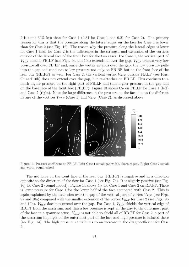
2 is some 30% less than for Case 1 (0.34 for Case 1 and 0.21 for Case 2). The primaryreason for this is that the pressure along the lateral edges on the face for Case 1 is lowerthan for Case 2 (see Fig. 12). The reason why the pressure along the lateral edges is lowerfor Case 1 than for Case 2 is the differences in the strength and extension of the vorticesoutside of the lateral face of the front box for the two cases. For Case 1, the vertical part ofVSLF outside FB LF (see Figs. 9a and 10a) extends all over the gap. VSLF creates very lowpressure all over FB LF and, since the vortex extends over the gap, the low pressure pullsinto the gap and conduces to low pressure not only on FB BF but on the front face of therear box (RB FF) as well. For Case 2, the vertical vortex VRLF outside FB LF (see Figs.9b and 10b) does not extend over the gap, but re-attaches on FB LF. This conduces to amuch higher pressure on the right part of FB LF and thus higher pressure in the gap andon the base face of the front box (FB BF). Figure 13 shows CP on FB LF for Case 1 (left)and Case 2 (right). Note the large difference in the pressure on the face due to the differentnature of the vortices VSLF (Case 1) and VRLF (Case 2), as discussed above.

CP

Figure 13: Pressure coefficient on FB LF. Left: Case 1 (small gap width, sharp edges). Right: Case 2 (smallgap width, round edges)

The net force on the front face of the rear box (RB FF) is negative and in a directionopposite to the direction of the flow for Case 1 (see Fig. 7c). It is slightly positive (see Fig.7c) for Case 2 (round model). Figure 14 shows CP for Case 1 and Case 2 on RB FF. Thereis lower pressure for Case 1 for the lower half of the face compared with Case 2. This isagain explained by the extension over the gap of the vertical part of vortex VSLF (see Figs.9a and 10a) compared with the smaller extension of the vortex VRLF for Case 2 (see Figs. 9band 10b). VRLF does not extend over the gap. For Case 1, VSLF shields the vertical edge ofRB FF from the airstream, and thus a low pressure is kept all the way to the outermost partof the face in a spanwise sense. VRLF is not able to shield all of RB FF for Case 2, a part ofthe airstream impinges on the outermost part of the face and high pressure is induced there(see Fig. 14). The high pressure contributes to an increase in the drag coefficient for Case2.

21

CP

Figure 14: Pressure coefficient on RB FF. Left: Case 1 (small gap width, sharp edges). Right: Case 2 (smallgap width, round edges).

3.4. Large gap width

This section describes the mean flow fields for the two cases with a large gap width (Case3 and Case 4). Some similarities and differences in the flow between small and large gapwidths are noted and analysed for the sharp and round models, respectively.

22

a)

VSLF

VSTF

VSG

UNS

FB FF

FB TF

FB LF

RB FF

b)

VRLF

VRTF

VRG

UNR

Figure 15: Streamlines of the time-averaged velocity projected onto the surface of the body (white lines)together with vortex cores (black drawn lines) and streamlines projected onto planes around vortex cores(black lines). a) Case 3 (large gap width, sharp edges). b) Case 4 (large gap width, round edges).

23

Figure 15a shows the system of vortical structures of the mean flow around Case 3(g/b = 0.67, sharp edges). Over the top face of the front box (FB TF) there’s a type ofvortex similar to VSTF for Case 1 (see Fig. 9a). The vortex over FB TF for Case 3 is calledVSTF as well in Fig. 15a. The vortex outside of the lateral face of the front box (FB LF) forCase 3 is called VSLF in Fig. 15a. As seen by comparing streamlines in plane z = 0.46 b inFigs. 10a (Case 1) and 10c (Case 3), vortex VSG is formed in the gap for Case 3 (g/b = 0.67,sharp edges). Vortex VSG is also pointed out in Fig. 15a, and it is a large horse-shoe likevortex. It extends horizontally in the gap and then down vertically in two tails outside thetwo connecting cylinders between the front and rear boxes. The mean flow in the gap iscompletely dominated by this vortex for Case 3. VSG (see Fig. 15a) is responsible for thelow pressure on FB BF (see Fig. 7a), contributing to an increase in CD for the whole modelfor Case 3. However, VSG is also responsible for the low pressure on the front face of therear box (RB FF, see Fig. 7c) which contributes to a decrease in CD for the entire model.

Figure 15b shows the vortex system around the model for Case 4 (g/b = 0.67, roundedges). The vortex outside of FB LF for Case 4 (VRLF ) is very similar to vortex VRLF (seeFig. 9b) outside FB LF for Case 2 (g/b = 0.17, round edges). The vortex above FB TFfor Case 4 is called VRTF in Fig. 15b. For Case 4 there is also a horse-shoe like vortex,VRG, that forms in the gap (see Fig. 15b), as for Case 3. Topologically, there is no largedifference in the flow in the gap for the two cases with large gap width. The gap is for bothcases dominated by the horse-shoe like vortices VSG and VRG, respectively (see streamlinesin plane z = 0.46 b in Figs. 10c and 10d). The vertical tails of VRG are however confinedto the space between the connecting cylinders between the front and rear boxes (see Fig.10d) while the tails of VSG are located outside the cylinders in a spanwise sense (see Figs.10c and 15a). CP for Case 3 and Case 4 on RB FF is presented in Fig. 17. Note the muchhigher pressure for Case 4 than for Case 3 on RB FF, indicating that VRG is weaker thanVSG.

24

a)

VSTF

b)

VRTF

c)

VSTF

VSG

d)

VRTF

VRG

Figure 16: Streamlines of the time-averaged velocity projected on plane y = 0. a) Case 1 (small gap width,sharp edges). b) Case 2 (small gap width, round edges). c) Case 3 (large gap width, sharp edges). d) Case4 (large gap width, round edges).

25

CP

Figure 17: Pressure coefficient on RB FF. Left: Case 3 (large gap width, sharp model). Right: Case 4 (largegap width, round model).

26

The difference between the contributions to CD (see Fig. 7c) from the front face of therear box (RB FF) between Case 3 and Case 4 is very large. Figure 7c shows that the contri-bution is slightly negative for Case 3 (-0.06). The contribution to CD from RB FF for Case4 is 0.467. The reason why the contributions from RB FF are so different between Case 3and Case 4 is the difference in the vortices formed in the gap in the two cases, VSG for Case3 (see Fig. 15a) and VRG for Case 4 (see Fig. 15b). Since the only geometrical differencebetween the Case 3 and Case 4 is the rounding of the leading edge on the front box, thelarge disparities between the cases in the gap flow are interesting. The difference is that,for Case 4, since VRG is confined between the connecting cylinders, it is not able to shieldRB FF from the airstream flowing along the lateral sides. For Case 3, the gap vortex, VSG,is located outside of the connecting cylinders and is much larger and stronger. This can beseen by comparing the streamlines around the vortices in plane z = 0.46b (see Figs. 10c and10d). Furthermore, the foci of VSG are also located further away from the base part of thefront box compared with the tails of VRG.

The above described difference between VSG and VRG has the consequence that, forCase 3, the gap vortex, VSG, is able to shield the exposed face, RB FF, from the airstreamimpinging, and thus a low pressure is kept in the gap and the contribution to CD from RB FFis negative for Case 3. For Case 4, however, the gap vortex VRG is not able to shield the frontface of the rear box (RB FF) and the airstream impinges on a larger area of RB FF andthus momentum is directly transferred from the free-streaming air to this exposed surface.The airstreams impinging on RB FF for Case 3 and Case 4 can also be seen by lookingat the two unstable nodes located in the upper corners of RB FF. The unstable nodes forCase 3 are denoted UNS (see Fig. 15a) and for Case 4 UNR (see Fig. 15b). UNR (Case4) are located closer to the midpoint of the face compared with the location of UNS (Case3). Thus the vertical parts (the tails) of VSG (Case 3) are able to shield the exposed face,RB FF, and direct the airstream around the face so that the air attaches on the lateral faceof the rear box instead. There is another fundemental difference between gap vortices VSG

and VRG. The former vortex is a result of the air separating on the leading edge on thefront box. This can be understood by looking at the streamlines projected in plane z = 46bin Fig. 10c) and in plane y = 0 in Fig. 16c. VRG is a result of the air separating on thebase edge of the front box (see Figs. 10d) and 16d). The air separates on the leading edge,re-attaches on the right part of FB LF and then separates again on the base lateral edge ofthe front box, and VRG is formed. The free-streaming air that flows outside of the FB LFvortex VRLF (see Fig. 15b) then confines VRG to the area between the connecting cylindersin the gap.

4. Conclusion

The LES was successfully employed to solve the flow around a simplified tractor-trailermodel. The model consisted of a tractor and a trailer separated by a gap and has previouslybeen investigated experimentally in a wind tunnel (Allan [1981]). Four different cases of themodel were studied. Two cases (Case 1 and Case 2) had a small gap width between the

27

tractor and the trailer. Case 1 had sharp leading edges on the front box and Case 2 hadrounded edges. The roundness of the leading edge was found to decrease the drag coefficientfor Case 2 in comparison with Case 1 in the same order of magnitude as in the referenceexperiments. The other two cases (Case 3 and Case 4) had a large gap width and Case 3had sharp leading edges on the front box and Case 4 had rounded. The drag coefficient forCase 3 increased slightly compared to the drag coefficient for Case 1 as expected from theexperimental results. The drag coefficient for Case 4 was expected to increase dramatically(in experiments, the increase was from 0.77 to 1.28). The increase of the drag coefficient forCase 4 compared with Case 2 was large in the present LES, but not as large as expected (insimulations, the increase was from 0.79 to 1.13). The main reason for this smaller increase inthe simulations compared to in the experiments was that the contribution to the drag coeffi-cient of the whole vehicle from the front face of the rear box (RB FF) was underpredicted inthe simulations (0.467 in LES compared with 0.677 in experiments). In general, the resultsfrom the two cases with sharp leading edge on the front box was in closer agreement to theexperimental values.

The mean flow fields around the four cases were described. For Case 1, the flow aroundthe front box and the gap was dominated by the vortices caused by the separation of theflow on the sharp leading edge on the front box. Almost all of the drag force on the vehiclewas taken up by the front box, and the resulting force on the rear box was close to zero.Rounding of the leading edges on the front box reduced the drag force of the front box andthus the whole vehicle for Case 2 for which the gap width was small. The flow field aroundthe front box and the gap for Case 2 was similar to the one around Case 1 but the roundnessof the leading edges on the front box caused much smaller vortices due separation than forCase 1. The difference in drag coefficient (1.022 and 0.793 for Case 1 and Case 2, respec-tively) was found to be mainly due to the decreased pressure along the curvature on therounded edges on the front box for Case 2. For the large gap width, the gain in decreaseddrag of the front box when rounding the leading edges was lost due to increased drag of therear box. It was shown that the reason for this was that the vortex formed outside of thelateral face of the front box in Case 4 was much smaller and could not shield the front faceof the rear box of the model from the oncoming flow.

The present work shows that LES can be used to gain knowledge about the flow struc-tures around simplified models of tractor-trailers which includes gap between the tractorand the trailer. This is a rather complex bluff body system that includes a number flow re-gions which are difficult to predict with CFD. These are e.g. separation of flow from roundededges, attached boundary layer flow on the trailer and interaction between the tractor andthe trailer. The computer expense of the simulations is managable due to the separatedcharacter of the flow. Without large regions of attached flow, the LES requirements fornear-wall resolution could be relaxed. Even though the Reynolds number in the presentstudy is rather high (0.51× 106 based on the height of the rear box), it is still one tenth ofthat of tractor-trailers on roads at operational speeds. With increasing Reynolds numbers,changes in the flow structures can be expected. Especially in the cases with rounded leading

28

edges on the front box. It has been seen in the present work that the drag coefficient ofthe model is very sensitive to the flow structures emanating from the separation from theleading edges. Thus, it can be expected that an increased Reynolds number will have largeinfluence on the drag coefficient as well. The present work shows how the flow structures af-fect the drag coefficient of the model. The comparison between simulated and experimentaldrag coefficients showed rather large disparities, especially for Case 4 with round edges onthe front box and large gap width. Important knowledge about the flow structures and howthey affect the drag coefficient and interact with the tractor and the trailer was obtained.

References

Allan, J., 1981. Aerodynamic drag and pressure measurements on a simplified tractor-trailer model. Journalof Wind Engineering and Industrial Aerodynamics 9, 125–136.

Arcas, D., Browand, F., Hammache, M., 2004. Flow structure in the gap between two bluff bodies. AIAAPaper 2004-2250.

AVL, 2009. CFD Solver. AVL Fire Manual, v2009.1, edition 04/2009.Barnard, R. H., 1996. Road Vehicle Aerodynamic Design, An Introduction, 1st Edition. Addison Wesley

Longman Limited, ISBN 0-582-24522-2.Cooper, K. R., 1985. The effect of front-edge rounding and rear edge shaping on the aerodynamic drag of

bluff vehicles in ground proximity. SAE Paper No. 850288.Cooper, K. R., 2002. Commercial vehicle aerodynamic drag reduction: Historical perspective as a guide. In:

The Aerodynamics of Heavy Vehicles: Trucks, Busses and Trains. Monterey, USA.Cooper, K. R., 2003. Truck aerodynamics reborn - lessons from the past. SAE Paper 2003-01-3376.Ghosal, S., Moin, P., 1995. The basic equations for the large eddy simulation of turbulent flows in complex

geometry. Journal of Computational Physics 118, 24–37.Hammache, M., Browand, F., 2002. On the aerodynamics of tractor-trailers. In: The Aerodynamics of Heavy

Vehicles: Trucks, Busses and Trains. Monterey, USA.Hemida, H., Krajnovic, S., Davidson, L., 2005. Large eddy simulations of the flow around a simplified

high speed train under the influence of cross-wind. In: 17th AIAA Computational Dynamics Conference.Toronto, Ontario, Canada.

Hucho, W.-H., 1998. Aerodynamics of Road Vehicles, 4th Edition. Society of Automotive Engineers, Inc.,ISBN 0-7680-0029-7.

Krajnovic, S., 2009. LES of flows around ground vehicles and other bluff bodies. Philosophical Transactionsof the Royal Society A 367 (1899), 2917–2930.

Krajnovic, S., 2011. Flow around a tall finite cylinder explored by large eddy simulation. Journal of FluidMechanics 676, 294–317.

Krajnovic, S., Davidson, L., 2003. Numerical study of the flow around the bus-shaped body. ASME: Journalof Fluids Engineering 125, 500–509.

Krajnovic, S., Davidson, L., 2005a. Flow around a simplified car, part 1: Large eddy simulation. ASME:Journal of Fluids Engineering 127, 907–918.

Krajnovic, S., Davidson, L., 2005b. Flow around a simplified car, part 2: Understanding the flow. ASME:Journal of Fluids Engineering 127, 919–928.

McCallen, R., Flowers, D., T. Dunn, J. O., Browand, F., Hammache, M., Leonard, A., Brady, M., Salari,K., Rutledge, W., Ross, J., Storms, B., Heineck, J. T., Driver, D., Bell, J., Walker, S., Zilliac, G., 2000.Aerodynamic drag of heavy vehicles (class 7-8): Simulation and benchmarking. SAE Paper 2000-01-2209.

Patankar, S., Spalding, D., 1972. A calculation procedure for heat, mass and momentum transfer in three-dimensional parabolic flows. Int. J. Heat Mass Transfer 15, 1787–1806.

Perry, A. E., Chong, M. S., 1987. A description of eddying motions and flow patterns using critical-pointconcepts. Ann. Rev. Fluid Mech. 19, 125 – 155.

Pope, S. B., 2000. Turbulent Flows, 1st Edition. Cambridge University Press, Cambridge.

29

Smagorinsky, J., 1963. General circulation experiments with the primitive equations. Monthly WeatherReview 91 (3), 99–165.

Sujudi, D., Haimes, R., 1995. Identification of swirling flow in 3-d vector fields. AIAA Paper 95-1715.

30