change detection in synthetic aperture radar images based...

IEEE TRANSACTIONS ON NEURAL NETWORKS AND LEARNING SYSTEMS, VOL. 27, NO. 1, JANUARY 2016 125

Change Detection in Synthetic Aperture RadarImages Based on Deep Neural Networks

Maoguo Gong, Senior Member, IEEE, Jiaojiao Zhao, Jia Liu, Qiguang Miao,and Licheng Jiao, Senior Member, IEEE

Abstract— This paper presents a novel change detectionapproach for synthetic aperture radar images based on deeplearning. The approach accomplishes the detection of the changedand unchanged areas by designing a deep neural network. Themain guideline is to produce a change detection map directlyfrom two images with the trained deep neural network. Themethod can omit the process of generating a difference image (DI)that shows difference degrees between multitemporal syntheticaperture radar images. Thus, it can avoid the effect of theDI on the change detection results. The learning algorithm fordeep architectures includes unsupervised feature learning andsupervised fine-tuning to complete classification. The unsuper-vised feature learning aims at learning the representation of therelationships between the two images. In addition, the supervisedfine-tuning aims at learning the concepts of the changed andunchanged pixels. Experiments on real data sets and theoreticalanalysis indicate the advantages, feasibility, and potential of theproposed method. Moreover, based on the results achieved byvarious traditional algorithms, respectively, deep learning canfurther improve the detection performance.

Index Terms— Deep learning, image change detection, neuralnetwork, synthetic aperture radar (SAR).

I. INTRODUCTION

IMAGE change detection is a process to identify thechanges that have occurred between the two images of the

same scene but taken at different times. It is an important issuein both civil and military fields. This depends on the fact that,for many public and private institutions, the knowledge of thedynamics of either natural resources or man-made structuresis a valuable source of information in decision making [1].It has found wide use in diverse disciplines, such as remotesensing, disaster evaluation, medical diagnosis, and videosurveillance [2]. In particular, when a natural catastrophestrikes, an effective and efficient change detection task appears

Manuscript received January 14, 2014; revised March 23, 2015 andMay 6, 2015; accepted May 16, 2015. Date of publication June 9, 2015; dateof current version December 17, 2015. This work was supported in part bythe National Nature Science Foundation of China under Grant 61273317 andGrant 61422209, in part by the National Program for Support of Top-NotchYoung Professionals of China, in part by the Specialized Research Fund forthe Doctoral Program of Higher Education under Grant 20130203110011, andin part by the Fundamental Research Funds for the Central Universities underGrant K5051202053.

M. Gong, J. Zhao, J. Liu, and L. Jiao are with the Key Laboratory ofIntelligent Perception and Image Understanding, Ministry of Education,Xidian University, Xi’an 710071, China (e-mail: [email protected];[email protected]; [email protected]; [email protected]).

Q. Miao is with the School of Computer Science and Technology,Xidian University, Xi’an 710071, China (e-mail: [email protected]).

Color versions of one or more of the figures in this paper are availableonline at http://ieeexplore.ieee.org.

Digital Object Identifier 10.1109/TNNLS.2015.2435783

critical when lives and properties are at stake. It proves tobe an important application of remote sensing technology.In particular, due to their independence on atmospheric andsunlight conditions, synthetic aperture radar (SAR) imageshave become valuable sources of information in changedetection. However, with the presence of the speckle noise,SAR images exhibit more difficulties than optical ones [3].

There are two major thoughts for change detection in SARimages according to the literature available. First, postclassi-fication comparison, which means separately classifying thetwo SAR images and then comparing their classificationresults to achieve the changed and unchanged regions [2], [4].This method has an advantage of avoiding radiationnormalization of multitemporal remote sensing images, whichare obtained from different sensors and different environmentalconditions. However, there exists an issue of accumulatedclassification error and a requirement for high accuracy ofclassifying each of the two images. Second, postcomparisonanalysis, that is to say that first making a difference image (DI)between multitemporal SAR images, and then analyzing itto gain change detection results. Thus, it is also calledDI analysis [5]. It is the current mainstream with excellentperformance. However, besides the method for analyzinga DI, the quality of a DI also affects the final detection results.

Most algorithms presented are based on the latterthought. The common technique to generate a DI is theratio method [6]. In addition, considering the influence ofspeckle noise, the log ratio is widely used [7], [8]. In theDI-analysis step, there are two conventional methods beingused, the thresholding method and the clustering method.Classical thresholding methods, such as [9] and [10], havebeen applied to determine the threshold in an unsupervisedmanner. Actually, in the thresholding method, it is necessaryto establish models to search for an optimal threshold.A Kittler-Illingworth (KI)-based method [Generalized Kittler-Illingworth method (GKI)] was generalized to take thenon-Gaussian distribution of the amplitude values of SARimages into account [1]. Among the most popular clusteringmethods, the fuzzy c-means algorithm (FCM) can retain moreinformation than hard clustering in some cases. In [5], weproposed an FCM-based SAR image change detection method[i.e., reformulated fuzzy local-information c-means algorithm(RFLICM)]. In recent years, graph cut [11], principalcomponent analysis [12], and Markov random field [13]are also increasingly applied to solve the change detectionproblem, but neural networks are rarely considered in the

2162-237X © 2015 IEEE. Personal use is permitted, but republication/redistribution requires IEEE permission.See http://www.ieee.org/publications_standards/publications/rights/index.html for more information.

126 IEEE TRANSACTIONS ON NEURAL NETWORKS AND LEARNING SYSTEMS, VOL. 27, NO. 1, JANUARY 2016

field. Just a few works were presented, such as a Hopfield-typeneural network proposed to model spatial correlations in [14]and a neural-network-based change-detection system formultispectral images in [15].

As mentioned above, change detection technology inSAR images has developed well. However, with dataacquisition channels and the scope of applications increasing,the involved algorithms cannot satisfy the requirementsfor higher accuracy and more flexible applications. As forthe widely used DI-analysis methods, there currently existthree problems in change detection as follows.

1) How to Suppress Speckle Noise? As an important char-acteristic of SAR images, speckle makes image detailsblurred and reduces intensity and spatial resolution ofimages, thus it is difficult to interpret SAR images.When changed information is extracted, the presenceof speckle results in some false alarms. Therefore,suppressing noise is a regular step before detectionand many algorithms have been produced to solve theproblem.

2) How to Generate a DI With Good Performance? TheDI-analysis method is regarded as an effective oneand used widely. The separability of a DI has directimpacts on classification results of the DI. It can beseen that a good DI is a prerequisite for the correctdetection.

3) How to Design an Efficient Classification Method? Thisis the most crucial step in the whole algorithm, whichdetermines the final change detection results.

Inspired by the architectural depth of the brain, deeplearning [16]–[19] has become a new kind of machine learningmethod and has been paid increasing attention in recent years.Deep learning algorithms seek to exploit the unknownstructure in the input distribution in order to discover goodrepresentations, with higher level learned features definedin terms of lower level features [20]. Convolutional neuralnetworks (CNNs) are the early proposed deep architectures.They are inspired by the receptive fields in neural cortex [21]mainly designed for 2-D data, such as images and videos. Withthe development of deep learning, both the frameworks andtraining algorithms of CNNs have been improved [22], [23].The breakthrough of the deep learning is a fast learningalgorithm for deep belief networks proposed in [24],a learning algorithm that greedily trains one layer at a time.They exploited the restricted Boltzmann machine (RBM) [25]and an unsupervised learning algorithm, for each layer. Shortlyafter, related algorithms based on autoencoders, which appar-ently exploit the same principle, were proposed [26]. Recently,regularization methods for deep networks have been proposedto improve the performance of the networks [27]–[29].Dropout training, whose key idea is to randomly dropunits from a neural network during training, significantlyreduces overfitting [27]. In addition, Goodfellow et al. [28]proposed maxout network. It is designed to both facilitateoptimization by dropout and improve the accuracy ofdropout’s fast approximate model averaging technique.Moreover, the benefit of a network with local winner-take-all blocks was demonstrated in [29]. Deep learning has

Fig. 1. Change detection problem.

important empirical successes in a number of traditionalartificial intelligence applications, such as natural languageprocessing [30] and image processing [31]–[33], especially theclassification [34]–[37] and recognition [38]–[41] tasks.

In this paper, we try to apply deep learning to SAR imagesrather than standard images. The proposed algorithm includesthree aspects as follows: 1) preclassification for obtaining somedata with labels of high accuracy; 2) constructing a deep neuralnetwork for learning images features, and then fine-tuning theparameters of the neural network; and 3) using the trained deepneural network for the classification of changed and unchangedpixels.

The rest of this paper is organized as follows. Section II willgive problem statements and the proposed algorithm frame-work. In Section III, the proposed method will be describedin detail. Section IV will present the experimental results onreal multitemporal SAR images to verify the feasibility ofthe method. Finally, the conclusion is drawn in Section V.

II. PROBLEM STATEMENTS AND

ALGORITHM FRAMEWORK

The two coregistered intensity SAR images I1 = {I1(i, j),1 ≤ i ≤ A, 1 ≤ j ≤ B} and I2 = {I2(i, j), 1 ≤ i ≤ A,1 ≤ j ≤ B} are considered, which have the same size A × Band are acquired over the same geographical area at two dif-ferent times t1 and t2, respectively. The two original imagesare polluted by noise. The change detection problem can beshown in Fig. 1. We should design efficient change detectionmethods to find the changes between the two images.

The procedure of commonly used change detection methodin SAR images can be divided into three steps: 1) imagepreprocessing; 2) generation of a DI; and 3) analysis of theDI [42]. The framework is shown in Fig. 2(a). In general,geometric correction and registration are usually implementedto align two images in the same coordinate frame beforechange detection. In the first step, it is only denoising that weneed to consider. As described in Section I, in the three steps,

GONG et al.: CHANGE DETECTION IN SAR IMAGES BASED ON DEEP NEURAL NETWORKS 127

Fig. 2. Algorithm frameworks for the change detection problem.(a) Framework based on DI-analysis. (b) Framework based on the proposeddeep neural networks.

every step is actually seen as a separate issue. Most previousstudies deal, respectively, with the three issues and proposedifferent algorithms for each issue, respectively. Our objectiveaims at simplifying the change detection issue without thetwo steps of filtering or generating a DI. The final detectionresults can be directly obtained from the two original images.Deep neural networks that have the powerful ability to learnthe complicated relationships from the two images prove to bethe first choice to realize the target. Fig. 2(b) shows a simpleframework of this method.

Here, we analyze the cause of choosing deep neuralnetworks. Shallow networks cannot efficiently represent thetask of interest [43]. The two original images without beingfiltered have complex relationships and we want to achievethe changes directly from the two images. Traditional deepneural networks would have sufficient representational powerto encode the task, but they are difficult to train because errorgradients decay exponentially with depth. We, therefore, adopta layerwise unsupervised pretraining strategy to train the deepnetwork. A deep architecture is composed of multiple levels ofnonlinear operations, such as in neural nets with many hiddenlayers, which is different from shallow neural networks. Deeplearning algorithms can discover multiple levels of distributedrepresentations, with higher levels representing more abstractconcepts. Automatically learning features without supervisionat multiple levels of abstraction allows a system to learncomplex functions, which maps the input to the outputdirectly from the data. For change detection issue, deepneural networks are able to learn the nonlinear relations fromthe two original images. There is no need to filter or generatea DI, which reaches the goal that we should enable changedetection process to be concise to some extent.

Change detection is often applied to disaster evaluation ormedical diagnosis. It is difficult to obtain the prior knowledge

Fig. 3. Flowchart of generating the deep neural network.

in these practical applications. Therefore, unsupervised changedetection methods are urgently needed and very important.Deep neural network is a method for unsupervised featurelearning and supervised classification. It can learn from thedata sets, which have a few labeled data. In addition, somelabeled data can be obtained by a preclassification. The flow-chart of generating the deep neural network is shown in Fig. 3.

III. METHODOLOGY

A. Preclassification and Sample Selection

To avoid generating a DI, we make a joint classificationof the two original images. Here, a joint classifier of thetwo original images based on FCM [joint classifier basedon FCM (JFCM)] is used. The method takes gray levels asinputs. The similarity of gray levels relating to two pixelsat the corresponding position in the two images is obtainedthrough similarity operator. Then, the global threshold valueof similarity is gotten, which is used to control the jointclassifier to classify the two images. The classification resultsare represented by � = {�1,�2}.

The specific process is shown in Algorithm 1. The similarityof gray levels relating to two pixels at the correspondingposition (i, j ) in the two original images is defined as

Si j =∣∣I 1

i j − I 2i j

∣∣

I 1i j + I 2

i j

(1)

where Si j ∈ [0, 1], and I ti j is the gray level at the position

(i, j ) in the t-temporal image (t = 1, 2). The global thresh-old value (T ) of similarity is gotten by iterative thresholdmethod [44]. The classifier determines reference points forclassification according to the principle of minimum variance.The variance at the position (i, j ) in the t-temporal image isgiven by

δti j = ωt

i j

(

I ti j − Gij

)2 (2)


Algorithm 1 Joint Classification Based on FCMInput: Two original images I1 and I2

Set end conditionswhile (! end conditions)

for each i ∈ [1, A] dofor each j ∈ [1, B] do

compute similarity of gray-levels Sij and variance

δ1ij, δ

2ij

if δ1ij ≤ δ2

ijclassify I 1

ij using FCM algorithmif Sij ≤ T // T is the global

threshold value of similarityΩ2

ij = Ω1ij

else classify I 2ij using FCM algorithm

end ifelse classify I 2

ij using FCM algorithmif Sij ≤ T

Ω1ij = Ω2

ijelse classify I 1

ij using FCM algorithmend if

end ifend for

end forend while

Output: � = {Ω1,Ω2}

where

ωti j = I t

i j /(

I 1i j + I 2

i j

)

(3)

Gij =2

∑

t=1

ωti j I t

i j (4)

where ωti j represents the weight of gray value and Gij repre-

sents the weighted average gray value. Therefore, (3) and (4)are substituted into (2) and δt

i j are also written by

δti j = I t

i j

I 1i j + I 2

i j

⎡

⎣I ti j −

(

I 1i j

)2 + (

I 2i j

)2

I 1i j + I 2

i j

⎤

⎦

2

. (5)

Derived from (1) and (5), we obtain the followingtwo equations:

δ1i j = I 2

i j

I 1i j I 2

i j

I 1i j + I 2

i j

[Si j ]2 (6)

δ2i j = I 1

i j

I 1i j I 2

i j

I 1i j + I 2

i j

[Si j ]2. (7)

If δ1i j ≥ δ2

i j , then I 1i j ≤ I 2

i j . Suppose that reference pointsfor classification are chosen according to the principle ofmaximum variance. I 1

i j is viewed as the reference point. WhenSi j ≤ T , �2

i j = �1i j and when Si j > T , �2

i j �= �1i j .

After a few iterations of classification, the category towhich I 2

i j belongs has a greater clustering center than the oneto which I 1

i j belongs. In this case, the possibility that changedinformation in different images has the same label increases,

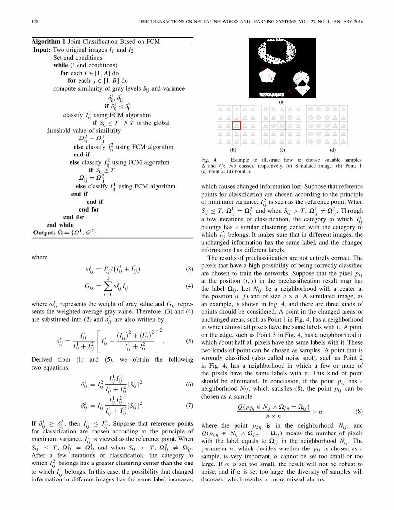
Fig. 4. Example to illustrate how to choose suitable samples.� and ©: two classes, respectively. (a) Simulated image. (b) Point 1.(c) Point 2. (d) Point 3.

which causes changed information lost. Suppose that referencepoints for classification are chosen according to the principleof minimum variance. I 2

i j is seen as the reference point. WhenSi j ≤ T , �1

i j = �2i j and when Si j > T , �1

i j �= �2i j . Through

a few iterations of classification, the category to which I 1i j

belongs has a similar clustering center with the category towhich I 2

i j belongs. It makes sure that in different images, theunchanged information has the same label, and the changedinformation has different labels.

The results of preclassification are not entirely correct. Thepixels that have a high possibility of being correctly classifiedare chosen to train the networks. Suppose that the pixel pi j

at the position (i, j ) in the preclassification result map hasthe label �i j . Let Nij be a neighborhood with a center atthe position (i, j ) and of size n × n. A simulated image, asan example, is shown in Fig. 4, and there are three kinds ofpoints should be considered. A point in the changed areas orunchanged areas, such as Point 1 in Fig. 4, has a neighborhoodin which almost all pixels have the same labels with it. A pointon the edge, such as Point 3 in Fig. 4, has a neighborhood inwhich about half all pixels have the same labels with it. Thesetwo kinds of point can be chosen as samples. A point that iswrongly classified (also called noise spot), such as Point 2in Fig. 4, has a neighborhood in which a few or none ofthe pixels have the same labels with it. This kind of pointshould be eliminated. In conclusion, if the point pi j has aneighborhood Nij , which satisfies (8), the point pi j can bechosen as a sample

Q(pξη ∈ Nij ∧ �ξη = �i j )

n × n> α (8)

where the point pξη is in the neighborhood Nij , andQ(pξη ∈ Nij ∧ �ξη = �i j ) means the number of pixelswith the label equals to �i j in the neighborhood Nij . Theparameter α, which decides whether the pi j is chosen as asample, is very important. α cannot be set too small or toolarge. If α is set too small, the result will not be robust tonoise; and if α is set too large, the diversity of samples willdecrease, which results in more missed alarms.


B. Deep Neural Network Establishment

Training a deep neural network is the core part of thealgorithm. It is difficult to optimize the weights and biasesin nonlinear networks, which have multiple hidden layers.Starting with random weights, multilayer BP network cannotalways find a satisfactory result. If the initial weights are large,the result typically traps into local optimization. However,small initial weights lead the gradients in the early layers tobe tiny, thus making it infeasible to train networks with manyhidden layers. The initial weights close to a good solutioncan make gradient descent works well, but finding such initialweights requires a very different type of algorithm that learnsone layer of features at a time. The RBM [37] can help tosolve the problem.

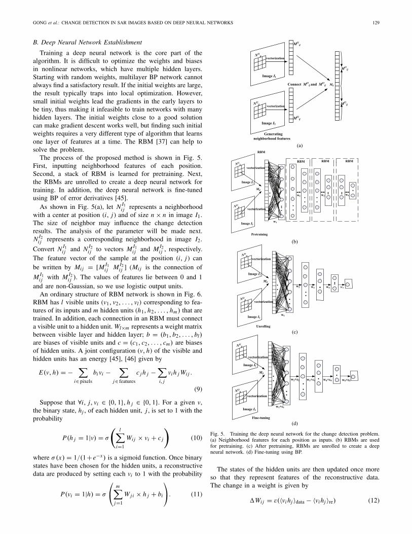
The process of the proposed method is shown in Fig. 5.First, inputting neighborhood features of each position.Second, a stack of RBM is learned for pretraining. Next,the RBMs are unrolled to create a deep neural network fortraining. In addition, the deep neural network is fine-tunedusing BP of error derivatives [45].

As shown in Fig. 5(a), let N I1i j represents a neighborhood

with a center at position (i, j ) and of size n × n in image I1.The size of neighbor may influence the change detectionresults. The analysis of the parameter will be made next.N I2

i j represents a corresponding neighborhood in image I2.

Convert N I1i j and N I2

i j to vectors M I1i j and M I2

i j , respectively.The feature vector of the sample at the position (i, j ) canbe written by Mij = [M I1

i j M I2i j ] (Mij is the connection of

M I1i j with M I2

i j ). The values of features lie between 0 and 1and are non-Gaussian, so we use logistic output units.

An ordinary structure of RBM network is shown in Fig. 6.RBM has l visible units (v1, v2, . . . , vl ) corresponding to fea-tures of its inputs and m hidden units (h1, h2, . . . , hm) that aretrained. In addition, each connection in an RBM must connecta visible unit to a hidden unit. Wl×m represents a weight matrixbetween visible layer and hidden layer; b = (b1, b2, . . . , bl)are biases of visible units and c = (c1, c2, . . . , cm) are biasesof hidden units. A joint configuration (v, h) of the visible andhidden units has an energy [45], [46] given by

E(v, h) = −∑

i∈ pixels

bi vi −∑

j∈ features

c j h j −∑

i, j

vi h j Wij .

(9)

Suppose that ∀i, j, vi ∈ {0, 1}, h j ∈ {0, 1}. For a given v,the binary state, hj , of each hidden unit, j , is set to 1 with theprobability

P(h j = 1|v) = σ

(l

∑

i=1

Wij × vi + c j

)

(10)

where σ(x) = 1/(1+e−x) is a sigmoid function. Once binarystates have been chosen for the hidden units, a reconstructivedata are produced by setting each vi to 1 with the probability

P(vi = 1|h) = σ

⎛

⎝

m∑

j=1

W ji × h j + bi

⎞

⎠. (11)

Fig. 5. Training the deep neural network for the change detection problem.(a) Neighborhood features for each position as inputs. (b) RBMs are usedfor pretraining. (c) After pretraining, RBMs are unrolled to create a deepneural network. (d) Fine-tuning using BP.

The states of the hidden units are then updated once moreso that they represent features of the reconstructive data.The change in a weight is given by

�Wij = ε(〈vi hj 〉data − 〈vi hj 〉re) (12)


Fig. 6. Structure of RBM.

where ε is a learning rate and 〈vi h j 〉data is the fraction fordata when the feature detectors are being driven by data,and 〈vi h j 〉re is the corresponding fraction for reconstructions.A simplified version of the same learning rule is used for thebiases.

A two-layer RBM network in which stochastic, binaryfeatures are connected to stochastic, binary feature detectorsusing symmetrically weighted connections can be used tomodel neighborhood features. The features correspond tovisible units of the RBM because their states are observed;the feature detectors correspond to hidden units. The networkassigns a probability to every possible pixel via this energyfunction in (9) [47]. Given the set of training samples, whichare chosen previously, a stack of RBM is used to pretraining.The pretraining does not use any information of the classlabels. Here, a layer-by-layer learning algorithm is applied.As shown in Fig. 5(b), the output of the upper layer istaken as the input of the next layer. Here, every layer is atwo-layer RBM network, which is trained according to therules described previously.

After pretraining, the RBM model is unfolded to producea deep neural network that initially uses the same weightsand biases, as shown in Fig. 5(c). The cross-entropy errorbackpropagation strategy is used through the whole networkto fine-tuned the weights for optimal classification, as shownin Fig. 5(d). The cross-entropy error is represented by

E = −∑

i

ei logei −∑

i

(1 − ei ) log(1 − ei ) (13)

where ei is the label of the sample i and ei is the classificationresult.

By training and fine-tuning the network, the final deepneural network is established. The neighborhood features ofeach position are fed into the deep neural network. In addition,the network outputs the class label of the pixel. The classlabel 0 represents the pixel being changed, and the class label 1represents the pixel being unchanged.

C. Feature Analysis and Denoising

Therefore, what features do the deep network learns andwhy can it perform well? During training of each layer,hidden layer is trained to represent the dominate factors ofthe data in visible layer. After being trained, the RBM givesa reliable representation of the input data statistically. Theknowledge of the input data is learned. In addition, in higherlayers, the knowledge is more abstract and helpful to predict

Fig. 7. Feature images extracted from hidden layers. (a) Input SAR image.(b)–(e) Feature images extracted from the first layer. (f)–(i) Feature imagesextracted from the second layer. (j)–(m) Feature images extracted from thethird layer.

the output. To observe the layerwise process clearly, we inputan SAR image, as shown in Fig. 7(a), and train the networkwithout supervision. Then, we extract typical features ofunits in each layer and draw the feature images, as shownin Fig. 7(b)–(m).

It can be seen in Fig. 7 that different hidden layers learndifferent features. In low layers, such as the first hidden layer,the features learned are simple shapes, including lines andpoints. Typically, Fig. 7(b) labels an obvious line in inputimage, Fig. 7(c) shows noises in an area, and Fig. 7(e) showsall the noises and a line. In the second layer, some structurefeatures are showed, but noises are obvious. In high layers,such as the third layer, the features are more complex thanthat in lower layers. Such as Fig. 7(k), it gets rid of theimpact of noise, but two different areas are recognized as one.In Fig. 7(m), it recognizes four areas, but it is corruptedby some unobvious noises. It can be seen that the deepnetwork finally learns the major features of the input imageand weaken the influence of noises. Deep learning appliesto not only standard images, which are the main datasources in the previous research, but also SAR images.Although SAR images have speckle noise that is very difficultto tackle.

The feature images, shown in Fig. 7, are typical featuresextracted from hidden layers. In addition, the actual numberof features is very large. A feature image can be seen as akind of interpretation of the input image. Maybe one kind ofinterpretation is not complete, but a large number of featurescan represent the image well. Therefore, the network hasgrasped the skill of how to interpret and represents the imageafter unsupervised learning. However, it has no idea what to


Fig. 8. Multitemporal images relating to Ottawa. (a) Image acquired inJuly 1997, during the summer flooding. (b) Image acquired in August 1997,after the summer flooding. (c) Ground truth.

Fig. 9. Multitemporal images relating to Yellow River Estuary. (a) Imageacquired in June 2008. (b) Image acquired in June 2009.

do with the features learned and how to deal with the image.Therefore, examples are needed.

IV. EXPERIMENTAL STUDY

A. Introduction to Data Sets

The Ottawa data set is a section (290 × 350 pixels)of two SAR images over the city of Ottawa acquired byRADARSAT SAR sensor and provided by the DefenceResearch and Development Canada, Ottawa. The availableground truth (reference image), which is shown in Fig. 8(c),was created by integrating prior information with photoin-terpretation based on the input images [Fig. 8(a) and (b)].The experiment on Ottawa data set is an instance of disasterevaluation. The changed areas represent the affected areas.

The Yellow River data set used in the experiments consistsof two SAR images acquired by Radarsat-2 at the region ofYellow River Estuary in China in June 2008 and June 2009,as shown in Fig. 9. It is worth noting that the two imagesare single-look image and four-look image, respectively. Thismeans that the influence of speckle noise on the imageacquired in 2008 is much greater than that of the one acquiredin 2009. The huge difference of speckle noise level betweenthe two images used may complicate the processing of changedetection. The original size of these two SAR images acquiredby Radarsat-2 is 7666 × 7692. They are too huge to show thedetail information in such small pages.

We select four typical areas (the Inland water, the coastline,and the two farmlands), where different kinds of changesoccur. Inland water where the changed areas are concentratedon the borderline of the river is shown in Fig. 10. It iscomparatively hard to detect. Fig. 11 shows the coastlinewhere the changed areas are relatively small, compared with

Fig. 10. Multitemporal images relating to Inland water of Yellow RiverEstuary. (a) Image acquired in June 2008. (b) Image acquired in June 2009.(c) Ground truth.

Fig. 11. Multitemporal images relating to Coastline of Yellow River Estuary.(a) Image acquired in June 2008. (b) Image acquired in June 2009. (c) Groundtruth.

Fig. 12. Multitemporal images relating to Farmland C of Yellow RiverEstuary. (a) Image acquired in June 2008. (b) Image acquired in June 2009.(c) Ground truth.

Fig. 13. Multitemporal images relating to Farmland D of Yellow RiverEstuary. (a) Iimage acquired in June 2008. (b) Image acquired in June 2009.(c) Ground truth.

the farmlands with large and regular changes. It can beseen that the changed areas appear as newly reclaimed farm-lands in Figs. 12 and 13, respectively. The experiments onYellow River data sets are instances of environmentalmonitoring. The changed areas show the changes on thesurface.

B. Evaluation Criteria

The quantitative analysis of change detection results is setas follows: 1) the false negatives (FNs) (changed pixels thatundetected) and 2) the false positives (FPs) (unchanged pixelswrongly detected as changed) should be calculated. Overallerror (OE) is the sum of FN and FP [48]. In the experiments,they are reported as percentages. We calculate the percentage


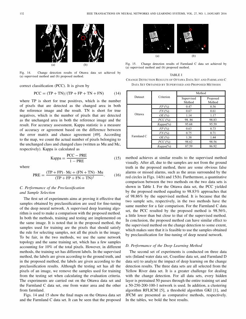
Fig. 14. Change detection results of Ottawa data set achieved by(a) supervised method and (b) proposed method.

correct classification (PCC). It is given by

PCC = (TP + TN)/(TP + FP + TN + FN) (14)

where TP is short for true positives, which is the numberof pixels that are detected as the changed area in boththe reference image and the result. TN is short for truenegatives, which is the number of pixels that are detectedas the unchanged area in both the reference image and theresult. For accuracy assessment, Kappa statistic is a measureof accuracy or agreement based on the difference betweenthe error matrix and chance agreement [49]. Accordingto the map, we count the actual number of pixels belonging tothe unchanged class and changed class (written as Mu and Mc,respectively). Kappa is calculated as

Kappa = PCC − PRE

1 − PRE(15)

where

PRE = (TP + FP) · Mc + (FN + TN) · Mu

(TP + FP + FN + TN)2 . (16)

C. Performance of the Preclassificationand Sample Selection

The first set of experiments aims at proving it effective thatsamples obtained by preclassification are used for fine-tuningof the deep neural network. A supervised deep learning algo-rithm is used to make a comparison with the proposed method.In both the methods, training and testing are implemented onthe same image. It is noted that in the proposed method, thesamples used for training are the pixels that should satisfythe rule for selecting samples, not all the pixels in the image.To be fair, in the two methods, we use the same networktopology and the same training set, which has a few samplesaccounting for 10% of the total pixels. However, in differentmethods, the training set has different labels. In the supervisedmethod, the labels are given according to the ground truth, andin the proposed method, the labels are given according to thepreclassification results. Although the testing set has all thepixels of an image, we remove the samples used for trainingfrom the testing set when calculating the evaluation criteria.The experiments are carried out on the Ottawa data set andthe Farmland C data set, one from water area and the otherfrom farmland.

Figs. 14 and 15 show the final maps on the Ottawa data setand the Farmland C data set. It can be seen that the proposed

Fig. 15. Change detection results of Farmland C data set achieved by(a) supervised method and (b) proposed method.

TABLE I

CHANGE DETECTION RESULTS OF OTTAWA DATA SET AND FARMLAND C

DATA SET OBTAINED BY SUPERVISED AND PROPOSED METHODS

method achieves at similar results to the supervised methodvisually. After all, due to the samples are not from the groundtruth in the proposed method, there are some obvious falsealarms or missed alarms, such as the areas surrounded by thered circles in Figs. 14(b) and 15(b). Furthermore, a quantitativecomparison between the two methods on the two data sets isshown in Table I. For the Ottawa data set, the PCC yieldedby the proposed method equaling to 98.83% approaches thatof 98.86% by the supervised method. It is because that thetwo sample sets, respectively, in the two methods have thesame number for a fair comparison. For the Farmland C dataset, the PCC resulted by the proposed method is 98.56%,a little lower than but close to that of the supervised method.In conclusion, the proposed method can have similar effect tothe supervised method on the change detection to some extent,which makes sure that it is feasible to use the samples obtainedby preclassification for fine-tuning of deep neural network.

D. Performance of the Deep Learning Method

The second set of experiments is conducted on three datasets (Inland water data set, Coastline data set, and Farmland Ddata set) to analyze the impact of deep learning on the changedetection results. The three data sets are all selected from theYellow River data set. It is a greater challenge for dealingwith the change detection. For all data sets, every hiddenlayer is pretrained 50 passes through the entire training set anda 50-250-200-100-1 network is used. In addition, a clusteringalgorithm RFLICM [5], a threshold algorithm GKI [1], andJFCM are presented as comparative methods, respectively.In the tables, we bold the best results.


Fig. 16. Change detection results of Inland water data set achieved by(a) GKI, (b) RFLICM, (c) JFCM, and (d) proposed method.

Fig. 17. Feature images of Inland water data set extracted from thethird layer.

1) Results on the Inland Water Data Set: The changedetection results generated by the proposed method and thethree comparative methods on the Inland water data set arepresented in Fig. 16. As shown in Fig. 16(a), the final mapgenerated by GKI is polluted by many white noise spots.It is due to the necessity of modeling data for searchingan optimal threshold in the GKI method. Any little error inthreshold may result in the presence of noise on the final map.As for RFLICM, there are also many noise spots emerging onthe black ground. Clustering methods are sensitive to noise.Although RFLICM, which incorporates both local spatial andgray information, is an improved method, it cannot give abest result in this case. Since the influence of the specklenoise on the Yellow River data set is much great. JFCM isused for preclassification just because a DI can be avoided.In the method, FCM is separately implemented on two originalimages. Although a joint-classification strategy is used, falsealarms or missed alarms are high. By contrast, the proposedmethod applying deep learning has an obvious improvement.In particular, it appears much effective without a DI generated.In Fig. 17, we exhibit some feature images extracted from thehighest hidden layer. It is clear that the deep network is ableto learn meaningful features and overcome the noise that ischaracteristic of SAR. The features learnt are local features andthe stacked RBMs can represent the difference features of thetwo images. In Fig. 17, different feature images have differentrepresentations and even some feature images highlight thechanged areas. Even if the two images have different looksof speckle, deep learning learns the meaningful features ofthe images and restricts the impact of noise. Furthermore,with reliably training samples, which are selected to avoidthe influence of noise, the method is robust. That is whyFP yielded by the proposed method is much lower. In Table II,the performances of the four methods are given quantitatively.The proposed method exhibits the best results.

TABLE II

CHANGE DETECTION RESULTS OF INLAND WATER DATA SET

Fig. 18. Change detection results of Coastline data set achieved by (a) GKI,(b) RFLICM, (c) JFCM, and (d) proposed method.

Fig. 19. Feature images of Coastline data set extracted from the third layer.

TABLE III

CHANGE DETECTION RESULTS OF COASTLINE DATA SET

2) Results on the Coastline Data Set: For the Coastlinedata set, Fig. 18 shows the final maps of the four methods.GKI presents the worst performance. The final map swarmswith many white spots. In Fig. 18(b), the final map obtainedby RFLICM has many false alarms because of the existenceof noise. As shown in the figure, the proposed method basedJFCM is the best to complete the detection task. Fig. 19 showssome features images learned by the network. It can be seenthat noises are not obvious. Moreover, quantitative analysisin Table III also declares this point. The PCC yielded bythe proposed method equals to 99.81% is higher than thatof 98.48% by JFCM, and has a big promotion. Serving as anoverall evaluation, PCC and Kappa of the proposed methodexhibit best among, although FN of it is not best. Besides, ourmethod has another advantage that it can result in lower FP.

3) Results on the Farmland D Data Set: The results ofthe experiments on the Farmland D data set are shownin Fig. 20 and listed in Table IV, respectively. The proposedmethod appears much better than the three other methods.In Table IV, our method exhibits the best PCC and Kappa.In all, the proposed method wins in the competition bothfrom the figure and from the table. For both the land andthe water areas, our method can present good performance.


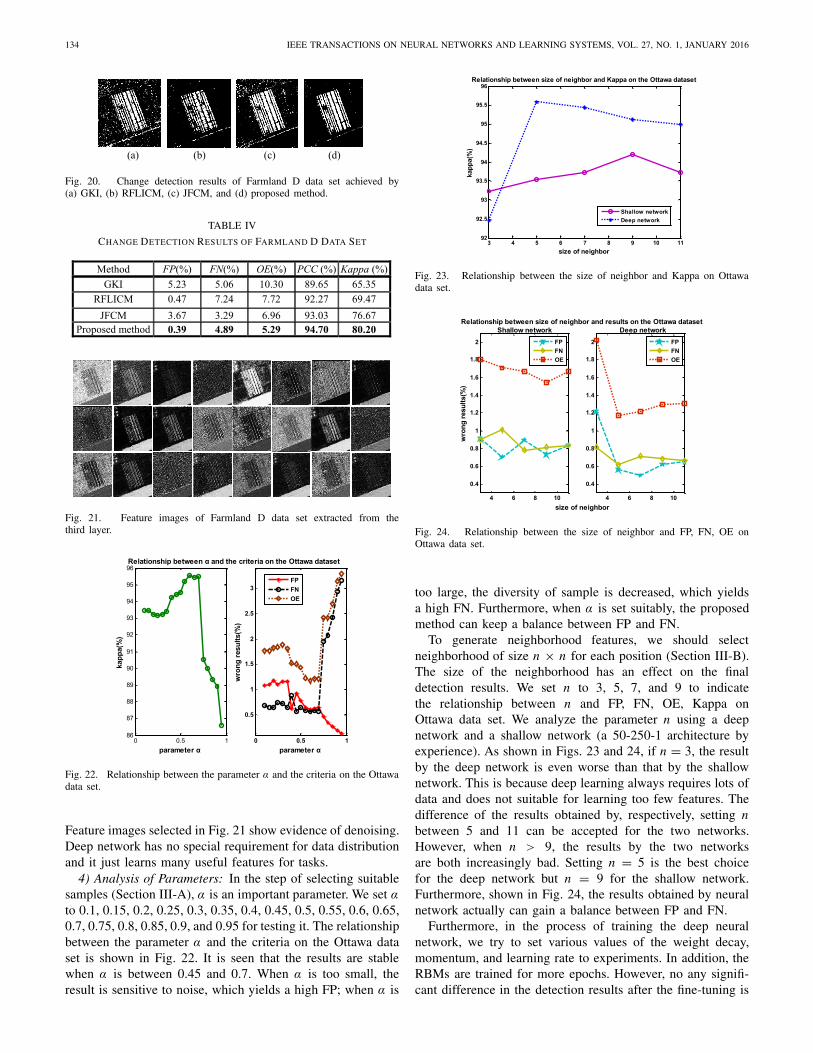
Fig. 20. Change detection results of Farmland D data set achieved by(a) GKI, (b) RFLICM, (c) JFCM, and (d) proposed method.

TABLE IV

CHANGE DETECTION RESULTS OF FARMLAND D DATA SET

Fig. 21. Feature images of Farmland D data set extracted from thethird layer.

Fig. 22. Relationship between the parameter α and the criteria on the Ottawadata set.

Feature images selected in Fig. 21 show evidence of denoising.Deep network has no special requirement for data distributionand it just learns many useful features for tasks.

4) Analysis of Parameters: In the step of selecting suitablesamples (Section III-A), α is an important parameter. We set αto 0.1, 0.15, 0.2, 0.25, 0.3, 0.35, 0.4, 0.45, 0.5, 0.55, 0.6, 0.65,0.7, 0.75, 0.8, 0.85, 0.9, and 0.95 for testing it. The relationshipbetween the parameter α and the criteria on the Ottawa dataset is shown in Fig. 22. It is seen that the results are stablewhen α is between 0.45 and 0.7. When α is too small, theresult is sensitive to noise, which yields a high FP; when α is

Fig. 23. Relationship between the size of neighbor and Kappa on Ottawadata set.

Fig. 24. Relationship between the size of neighbor and FP, FN, OE onOttawa data set.

too large, the diversity of sample is decreased, which yieldsa high FN. Furthermore, when α is set suitably, the proposedmethod can keep a balance between FP and FN.

To generate neighborhood features, we should selectneighborhood of size n × n for each position (Section III-B).The size of the neighborhood has an effect on the finaldetection results. We set n to 3, 5, 7, and 9 to indicatethe relationship between n and FP, FN, OE, Kappa onOttawa data set. We analyze the parameter n using a deepnetwork and a shallow network (a 50-250-1 architecture byexperience). As shown in Figs. 23 and 24, if n = 3, the resultby the deep network is even worse than that by the shallownetwork. This is because deep learning always requires lots ofdata and does not suitable for learning too few features. Thedifference of the results obtained by, respectively, setting nbetween 5 and 11 can be accepted for the two networks.However, when n > 9, the results by the two networksare both increasingly bad. Setting n = 5 is the best choicefor the deep network but n = 9 for the shallow network.Furthermore, shown in Fig. 24, the results obtained by neuralnetwork actually can gain a balance between FP and FN.

Furthermore, in the process of training the deep neuralnetwork, we try to set various values of the weight decay,momentum, and learning rate to experiments. In addition, theRBMs are trained for more epochs. However, no any signifi-cant difference in the detection results after the fine-tuning is


Fig. 25. Change detection results of Ottawa data set achieved by (a) RFLICM,(b) GKI, (c) LFS_KGC, (d) MRFFCM, (e) D_RFLICM, (f) D_GKI,(g) D_LFS_KGC, and (h) D_MRFFCM.

TABLE V

VALUES OF EVALUATION CRITERIA OF OTTAWA DATA SET

observed when the depth of the network is given. As statedin [47], the precise weights found by the greedy pretraining donot matter as long as it finds a good region from which to startthe fine-tuning. Such a problem that BP is easily to trap intolocal optimal can be avoided and the adjustment of parametersbecomes less complicated. As for the depth configuration andevery layer size, they are selected based on experience andmany experiments. Our data sets are not enough large to callfor more layers. We try different layer size, and actually theresults have no much difference. In the experiments, we usea deep network with a 50-250-200-100-1 architecture and ashallow network with a 50-250-1 architecture.

E. Flexibility of the Proposed Deep Learning Algorithm

The third set of experiments is carried out on all thefive data sets. Since deep learning algorithm contains asupervised fine-tuning stage, we can select some samplesfrom the results obtained by the available algorithms, suchas improved FCM algorithm based on Markov random field(MRFFCM) [13], GKI [1], RFLICM [5], and local fit-searchmodel (LFS)_kernel-induced graph cuts (KGC) [11], respec-tively. We make a comparison between the four methods andthe proposed algorithm based on the results obtained by thefour methods.

1) Results on the Ottawa Data Set: As for the Ottawa dataset, the results are shown in Fig. 25 and listed in Table V.

Fig. 26. Change detection results of Inland water data set achieved by(a) RFLICM, (b) GKI, (c) LFS_KGC, (d) MRFFCM, (e) D_RFLICM,(f) D_GKI, (g) D_LFS_KGC, and (h) D_MRFFCM.

Fig. 27. Change detection results of Coastline data set achieved by(a) RFLICM, (b) GKI, (c) LFS_KGC, (d) MRFFCM, (e) D_RFLICM,(f) D_GKI, (g) D_LFS_KGC, and (h) D_MRFFCM.

The influence of noise on the Ottawa data set is less great.Therefore, RFLICM, which applies local information, actuallyreduces the noise but causes the loss of details, as shownin Fig. 25(a). In addition, the FN yielded by RFLICM is ashigh as 2.49%. The proposed method based on the results ofRFLICM performs better with the fact that the four criteria areimproved. GKI, which needs to establish a model, is sensitiveto the noise. It yields a very high FP. The proposed methodbased on the results of GKI can balance FP and FN, andsignificantly reduces OE. As for LFS_KGC, it can decreasethe influence of speckle noise to some extent but would lead topoor results at the boundaries. The changed areas detected byLFS_KGC always have a good continuation and the final mapgenerated by it has little discrete noise. Therefore, from thevision, the change detection map is good. It yields the highestFP and OE, as shown in Table V. The proposed method basedon the result of LFS_KGC presents a better performance.MRFFCM is a clustering method with a modified MRF energyfunction. It can perform well on the Ottawa data set, which isinfluenced by noise less greatly. The proposed method basedon the result of MRFFCM outperforms the other methods.

In all, the proposed method based on the results obtained bythe available algorithms, respectively, arrives at significantlyimproved results. The deep learning algorithm has a strongcapacity of learning features and can interpret imagessufficiently. It can find a balance between denoising and


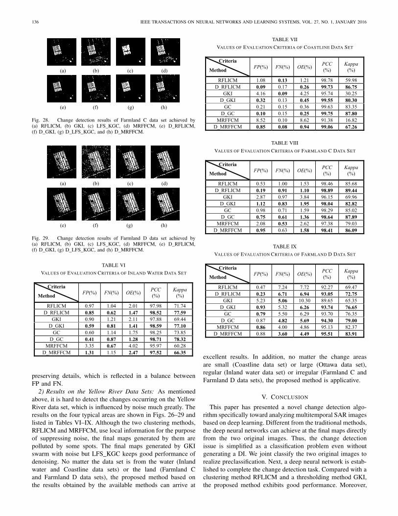
Fig. 28. Change detection results of Farmland C data set achieved by(a) RFLICM, (b) GKI, (c) LFS_KGC, (d) MRFFCM, (e) D_RFLICM,(f) D_GKI, (g) D_LFS_KGC, and (h) D_MRFFCM.

Fig. 29. Change detection results of Farmland D data set achieved by(a) RFLICM, (b) GKI, (c) LFS_KGC, (d) MRFFCM, (e) D_RFLICM,(f) D_GKI, (g) D_LFS_KGC, and (h) D_MRFFCM.

TABLE VI

VALUES OF EVALUATION CRITERIA OF INLAND WATER DATA SET

preserving details, which is reflected in a balance betweenFP and FN.

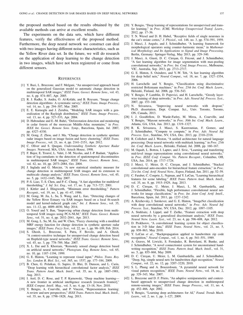
2) Results on the Yellow River Data Sets: As mentionedabove, it is hard to detect the changes occurring on the YellowRiver data set, which is influenced by noise much greatly. Theresults on the four typical areas are shown in Figs. 26–29 andlisted in Tables VI–IX. Although the two clustering methods,RFLICM and MRFFCM, use local information for the purposeof suppressing noise, the final maps generated by them arepolluted by some spots. The final maps generated by GKIswarm with noise but LFS_KGC keeps good performance ofdenoising. No matter the data set is from the water (Inlandwater and Coastline data sets) or the land (Farmland Cand Farmland D data sets), the proposed method based onthe results obtained by the available methods can arrive at

TABLE VII

VALUES OF EVALUATION CRITERIA OF COASTLINE DATA SET

TABLE VIII

VALUES OF EVALUATION CRITERIA OF FARMLAND C DATA SET

TABLE IX

VALUES OF EVALUATION CRITERIA OF FARMLAND D DATA SET

excellent results. In addition, no matter the change areasare small (Coastline data set) or large (Ottawa data set),regular (Inland water data set) or irregular (Farmland C andFarmland D data sets), the proposed method is applicative.

V. CONCLUSION

This paper has presented a novel change detection algo-rithm specifically toward analyzing multitemporal SAR imagesbased on deep learning. Different from the traditional methods,the deep neural networks can achieve at the final maps directlyfrom the two original images. Thus, the change detectionissue is simplified as a classification problem even withoutgenerating a DI. We joint classify the two original images torealize preclassification. Next, a deep neural network is estab-lished to complete the change detection task. Compared with aclustering method RFLICM and a thresholding method GKI,the proposed method exhibits good performance. Moreover,


the proposed method based on the results obtained by theavailable methods can arrive at excellent results.

The experiments on the data sets, which have differentfeatures, verify the effectiveness of the proposed method.Furthermore, the deep neural network we construct can dealwith two images having different noise characteristics, such asthe Yellow River data set. In the future, we will do researchon the application of deep learning to the change detectionin two images, which have not been registered or come fromdifferent sensors.

REFERENCES

[1] Y. Bazi, L. Bruzzone, and F. Melgani, “An unsupervised approach basedon the generalized Gaussian model to automatic change detection inmultitemporal SAR images,” IEEE Trans. Geosci. Remote Sens., vol. 43,no. 4, pp. 874–887, Apr. 2005.

[2] R. J. Radke, S. Andra, O. Al-Kofahi, and B. Roysam, “Image changedetection algorithms: A systematic survey,” IEEE Trans. Image Process.,vol. 14, no. 3, pp. 294–307, Mar. 2005.

[3] E. E. Kuruoglu and J. Zerubia, “Modeling SAR images with a gen-eralization of the Rayleigh distribution,” IEEE Trans. Image Process.,vol. 13, no. 4, pp. 527–533, Apr. 2004.

[4] D. Haboudane and E.-M. Bahri, “Deforestation detection and monitoringin cedar forests of the moroccan Middle-Atlas mountains,” in Proc.IEEE Int. Geosci. Remote Sens. Symp., Barcelona, Spain, Jul. 2007,pp. 4327–4330.

[5] M. Gong, Z. Zhou, and J. Ma, “Change detection in synthetic apertureradar images based on image fusion and fuzzy clustering,” IEEE Trans.Image Process., vol. 21, no. 4, pp. 2141–2151, Apr. 2012.

[6] C. Oliver and S. Quegan, Understanding Synthetic Aperture RadarImages. Norwood, MA, USA: Artech House, 1998.

[7] F. Bujor, E. Trouvé, L. Valet, J.-M. Nicolas, and J.-P. Rudant, “Applica-tion of log-cumulants to the detection of spatiotemporal discontinuitiesin multitemporal SAR images,” IEEE Trans. Geosci. Remote Sens.,vol. 42, no. 10, pp. 2073–2084, Oct. 2004.

[8] J. Inglada and G. Mercier, “A new statistical similarity measure forchange detection in multitemporal SAR images and its extension tomultiscale change analysis,” IEEE Trans. Geosci. Remote Sens., vol. 45,no. 5, pp. 1432–1445, May 2007.

[9] P.-S. Liao, T.-S. Chen, and P.-C. Chung, “A fast algorithm for multilevelthresholding,” J. Inf. Sci. Eng., vol. 17, no. 5, pp. 713–727, 2001.

[10] J. Kittler and J. Illingworth, “Minimum error thresholding,” PatternRecognit., vol. 19, no. 1, pp. 41–47, 1986.

[11] M. Gong, M. Jia, L. Su, S. Wang, and L. Jiao, “Detecting changes ofthe Yellow River Estuary via SAR images based on a local fit-searchmodel and kernel-induced graph cuts,” Int. J. Remote Sens., vol. 35,nos. 11–12, pp. 4009–4030, May 2014.

[12] O. Yousif and Y. Ban, “Improving urban change detection from multi-temporal SAR images using PCA-NLM,” IEEE Trans. Geosci. RemoteSens., vol. 51, no. 4, pp. 2032–2041, Apr. 2013.

[13] M. Gong, L. Su, M. Jia, and W. Chen, “Fuzzy clustering with a modifiedMRF energy function for change detection in synthetic aperture radarimages,” IEEE Trans. Fuzzy Syst., vol. 22, no. 1, pp. 98–109, Feb. 2014.

[14] S. Ghosh, L. Bruzzone, S. Patra, F. Bovolo, and A. Ghosh,“A context-sensitive technique for unsupervised change detection basedon Hopfield-type neural networks,” IEEE Trans. Geosci. Remote Sens.,vol. 45, no. 3, pp. 778–789, Mar. 2007.

[15] X. L. Dai and S. Khorram, “Remotely sensed change detection basedon artificial neural networks,” Photogram. Eng. Remote Sens., vol. 65,no. 10, pp. 1187–1194, 1999.

[16] G. E. Hinton, “Learning to represent visual input,” Philos. Trans. Roy.Soc. London B, Biol. Sci., vol. 365, no. 1537, pp. 177–184, 2009.

[17] B. Chen, G. Polatkan, G. Sapiro, D. Blei, D. Dunson, and L. Carin,“Deep learning with hierarchical convolutional factor analysis,” IEEETrans. Pattern Anal. Mach. Intell., vol. 35, no. 8, pp. 1887–1901,Aug. 2013.

[18] I. Arel, D. C. Rose, and T. P. Karnowski, “Deep machine learning—A new frontier in artificial intelligence research [research frontier],”IEEE Comput. Intell. Mag., vol. 5, no. 4, pp. 13–18, Nov. 2010.

[19] Y. Bengio, A. Courville, and P. Vincent, “Representation learning:A review and new perspectives,” IEEE Trans. Pattern Anal. Mach. Intell.,vol. 35, no. 8, pp. 1798–1828, Aug. 2013.

[20] Y. Bengio, “Deep learning of representations for unsupervised and trans-fer learning,” in Proc. ICML Workshop Unsupervised Transf. Learn.,2012, pp. 17–36.

[21] T. N. Wiesel and D. H. Hubel, “Receptive fields of single neurones inthe cat’s striate cortex,” J. Physiol., vol. 148, no. 3, pp. 574–591, 1959.

[22] J. Masci, J. Angulo, and J. Schmidhuber, “A learning framework formorphological operators using counter–harmonic mean,” in Mathemat-ical Morphology and Its Applications to Signal and Image Processing.Berlin, Germany: Springer-Verlag, May 2013, pp. 329–340.

[23] J. Masci, A. Giusti, D. C. Ciresan, G. Fricout, and J. Schmidhuber,“A fast learning algorithm for image segmentation with max-poolingconvolutional networks,” in Proc. Int. Conf. Image Process., Melbourne,VIC, Australia, Sep. 2013, pp. 2713–2717.

[24] G. E. Hinton, S. Osindero, and Y.-W. Teh, “A fast learning algorithmfor deep belief nets,” Neural Comput., vol. 18, no. 7, pp. 1527–1554,2006.

[25] H. Larochelle and Y. Bengio, “Classification using discriminativerestricted Boltzmann machines,” in Proc. 25th Int. Conf. Mach. Learn.,Helsinki, Finland, Jul. 2008, pp. 536–543.

[26] Y. Bengio, P. Lamblin, D. Popovici, and H. Larochelle, “Greedy layer-wise training of deep networks,” in Proc. Adv. Neural Inf. Process. Syst.,2007, pp. 153–160.

[27] N. Srivastava, “Improving neural networks with dropout,”Ph.D. dissertation, Dept. Comput. Sci., Univ. Toronto, Toronto,ON, Canada, 2013.

[28] I. J. Goodfellow, D. Warde-Farley, M. Mirza, A. Courville, andY. Bengio, “Maxout networks,” in Proc. 30th Int. Conf. Mach. Learn.,Atlanta, GA, USA, Jun. 2013, pp. 1319–1327.

[29] R. K. Srivastava, J. Masci, S. Kazerounian, F. Gomez, andJ. Schmidhuber, “Compete to compute,” in Proc. Adv. Neural Inf.Process. Syst., Stateline, NV, USA, Dec. 2013, pp. 2310–2318.

[30] R. Collobert and J. Weston, “A unified architecture for natural languageprocessing: Deep neural networks with multitask learning,” in Proc. 25thInt. Conf. Mach. Learn., Helsinki, Finland, Jul. 2008, pp. 160–167.

[31] M. Oquab, L. Bottou, I. Laptev, and J. Sivic, “Learning and transferringmid-level image representations using convolutional neural networks,”in Proc. IEEE Conf. Comput. Vis. Pattern Recognit., Columbus, OH,USA, Jun. 2014, pp. 1717–1724.

[32] J. Masci, U. Meier, D. C. Ciresan, and J. Schmidhuber, “Stackedconvolutional auto-encoders for hierarchical feature extraction,” in Proc.21st Int. Conf. Artif. Neural Netw., Espoo, Finland, Jun. 2011, pp. 52–59.

[33] C. Farabet, C. Couprie, L. Najman, and Y. LeCun, “Learning hierarchicalfeatures for scene labeling,” IEEE Trans. Pattern Anal. Mach. Intell.,vol. 35, no. 8, pp. 1915–1929, Aug. 2013.

[34] D. C. Ciresan, U. Meier, J. Masci, L. M. Gambardella, andJ. Schmidhuber, “Flexible, high performance convolutional neural net-works for image classification,” in Proc. Int. Joint Conf. Artif. Intell.,Barcelona, Spain, Jul. 2011, pp. 1237–1242.

[35] A. Krizhevsky, I. Sutskever, and G. E. Hinton, “ImageNet classificationwith deep convolutional neural networks,” in Proc. Adv. Neural Inf.Process. Syst., Stateline, NV, USA, Dec. 2012, pp. 1097–1105.

[36] A. Stuhlsatz, J. Lippel, and T. Zielke, “Feature extraction with deepneural networks by a generalized discriminant analysis,” IEEE Trans.Neural Netw. Learn. Syst., vol. 23, no. 4, pp. 596–608, Apr. 2012.

[37] D. Prokhorov, “A convolutional learning system for object classifica-tion in 3-D lidar data,” IEEE Trans. Neural Netw., vol. 21, no. 5,pp. 858–863, May 2010.

[38] Y. LeCun et al., “Backpropagation applied to handwritten zip coderecognition,” Neural Comput., vol. 1, no. 4, pp. 541–551, 1989.

[39] A. Graves, M. Liwicki, S. Fernández, R. Bertolami, H. Bunke, andJ. Schmidhuber, “A novel connectionist system for unconstrained hand-writing recognition,” IEEE Trans. Pattern Anal. Mach. Intell., vol. 31,no. 5, pp. 855–868, May 2009.

[40] D. C. Ciresan, U. Meier, L. M. Gambardella, and J. Schmidhuber,“Deep, big, simple neural nets for handwritten digit recognition,” NeuralComput., vol. 22, no. 12, pp. 3207–3220, 2010.

[41] S. L. Phung and A. Bouzerdoum, “A pyramidal neural network forvisual pattern recognition,” IEEE Trans. Neural Netw., vol. 18, no. 2,pp. 329–343, Mar. 2007.

[42] L. Bruzzone and D. F. Prieto, “An adaptive semiparametric and context-based approach to unsupervised change detection in multitemporalremote-sensing images,” IEEE Trans. Image Process., vol. 11, no. 4,pp. 452–466, Apr. 2002.

[43] Y. Bengio, “Learning deep architectures for AI,” Found. Trends Mach.Learn., vol. 2, no. 1, pp. 1–127, 2009.


[44] M. Sezgin and B. Sankur, “Survey over image thresholding techniquesand quantitative performance evaluation,” J. Electron. Imag., vol. 13,no. 1, pp. 146–168, 2004.

[45] G. E. Hinton and R. R. Salakhutdinov, “Reducing the dimensionality ofdata with neural networks,” Science, vol. 313, no. 5786, pp. 504–507,2006.

[46] G. E. Hinton, “A practical guide to training restricted Boltzmannmachines,” Dept. Comput. Sci., Univ. Toronto, Toronto, ON, USA,Tech. Rep. UTML TR 2010-003, Aug. 2010.

[47] G. E. Hinton and R. R. Salakhutdinov, “Reducing the dimensionality ofdata with neural networks,” Science, vol. 313, no. 5786, pp. 504–507,2006.

[48] P. L. Rosin and E. Ioannidis, “Evaluation of global image threshold-ing for change detection,” Pattern Recognit. Lett., vol. 24, no. 14,pp. 2345–2356, 2003.

[49] G. H. Rosenfield and K. Fitzpatrick-Lins, “A coefficient of agreement asa measure of thematic classification accuracy,” Photogram. Eng. RemoteSens., vol. 52, no. 2, pp. 223–227, 1986.

Maoguo Gong (M’07–SM’14) received theB.S. degree in electronic engineering andthe Ph.D. degree in electronic science andtechnology from Xidian University, Xi’an, China,in 2003 and 2009, respectively.

He has been a Teacher with Xidian University,since 2006, where he was promoted to AssociateProfessor and Full Professor, both with exceptiveadmission, in 2008 and 2010. He has authoredover 50 papers in journals and conferences, andholds 14 granted patents. His current research

interests include computational intelligence with applications to optimization,learning, data mining, and image understanding.

Dr. Gong received the prestigious National Program for the support ofTop-Notch Young Professionals from the Central Organization Department ofChina, the Excellent Young Scientist Foundation from the National NaturalScience Foundation of China, and the New Century Excellent Talent inUniversity from the Ministry of Education of China. He is the Vice Chairof the IEEE Computational Intelligence Society Task Force on MemeticComputing, an Executive Committee Member of the Chinese Associationfor Artificial Intelligence, and a Senior Member of the Chinese ComputerFederation.

Jiaojiao Zhao received the B.S. degree inelectronic engineering from Xidian University,Xi’an, China, in 2012, where she is currentlypursuing the M.S. degree with the School ofElectronic Engineering.

Her current research interests include changedetection in remote sensing images.

Jia Liu received the B.S. degree in electronicengineering from Xidian University, Xi’an, China,in 2013, where he is currently pursuing thePh.D. degree in pattern recognition and intelligentsystems with the School of Electronic Engineering.

His current research interests include computa-tional intelligence and image understanding.

Qiguang Miao received the M.Eng. andPh.D. degrees in computer science from XidianUniversity, Xi’an, China.

He is currently a Professor with the Schoolof Computer Science and Technology, XidianUniversity. His current research interests includeintelligent image processing and multiscalegeometric representations for images.

Licheng Jiao (SM’89) received the B.S. degree fromShanghai Jiao Tong University, Shanghai, China,in 1982, and the M.S. and Ph.D. degrees from Xi’anJiaotong University, Xi’an, China, in 1984 and 1990,respectively.

He has been a Professor with the School ofElectronic Engineering, Xidian University, Xi’an,since 1992. His current research interests includeimage processing, natural computation, machinelearning, and intelligent information processing.

change detection in synthetic aperture radar images based...

Documents