changing patterns of manufacturing growth … · we will try to trace effects of the changing...

CHANGING PATTERNS OF

MANUFACTURING GROWTH

A Decomposition Analysisof Location and Growth of

Manufacturing Industries in Denmark

By

Jens Lehrmann Rasmussenand

Søren Caspersen

Institute of Local Government Studies (AKF)Denmark

Nyropsgade 37DK 1602 Copenhagen V

Phone: +45 33 11 03 00Fax: +45 33 15 28 75

e-mail: Error! Bookmark not defined., Error! Bookmark not defined.Homepage: Error! Bookmark not defined.

Paper to be presented at the ERSA conference

REGIONAL COHESION AND COMPETITIVENESS IN21st CENTURY EUROPE

in the workshop

SPATIAL MODEL AND ANALYSIS

Copenhagen, June 1999

21

2

Abstract.

Industrial development in Denmark during the last decades has been characterisedby a remarkable change of spatial location of several industries. Among these,perhaps the most significant change has taken place in the manufacturingindustries. Where formerly most manufacturing firms were located in the citiesand towns of the Eastern and middle part of the country, recent decades havebeen hard on sunset industries like shipyards and breweries, where employmenthas declined markedly. In the Western part of the country, however, employmentand incomes in manufacturing industries has increased, primarily in industrieslike textiles and furniture manufacturing.

This paper presents an analysis of these changes and their effects on the distribution ofemployment and incomes in Denmark. The analysis will be based on the interregionalmodel LINE, developed in the Institute of Local Government Studies. LINE isdesigned to model economic activity within and between all 275 municipalities ofDenmark.

The central part of the analysis will be a decomposition of changes ofincome. This decomposition will show what parts of changes of income that areattributable to changes of employment, productivity, relative prices, etc., inmanufacturing industries. By means of LINE, such decomposition is carried out for allmunicipalities, and results are presented for diverse regions, and fordifferent types of municipalities, such as rural, peripheral, etc.

Among the finding is a confirmation that manufacturing industries have beeninstrumental in the relative prosperity that has been found in rural areas.An often heard hypothesis that a weaker performance of the peripheralregions of the country is attributable to a relative decline in manufacturingindustries is not confirmed by our findings.

31

3

1. Introduction.

Spatial location of industries has changed substantially in many countries during the

last decades. In very broad terms, the trends indicated consist in a decline in

manufacturing activities and an increase in service activities in urban areas and,

correspondingly, an increase in manufacturing activities in rural areas.

In a different set-up, the same tendency may be said to appear when it comes to

international location of industries, where manufacturing plants of transnational

companies are established in developing countries, and financial and other services

gain importance in the metropolitan areas of the rich countries. These tendencies are

directly linked to ongoing globalisation. Manufacturing growth in rural areas of rich

countries may be linked to globalisation in less obvious ways, or may have preceded it.

In Denmark relocation has been particularly important in manufacturing industries.

From the beginning of industrialisation in late nineteenth century, most manufacturing

plants have been located around Copenhagen and other cities. As no mineral extraction

took place, and no similar activities could compete with the cities for industrial

location, manufacturing activities tended to agglomerate in and around the existing

cities in Eastern and Central Denmark. In the cities, growing industries found markets

and infrastructure such as seaports and railways. As a consequence, urbanisation

followed industrial growth, and left Denmark in the middle of this century with a major

concentration of manufacturing industries and population in the Copenhagen

Metropolitan Region (CMR) and a few other cities (Jensen-Butler 1992).

21

2

This has changed markedly since then. Manufacturing growth has, until very recently,

primarily taken place in the more peripheral areas of Denmark, first of all in Jutland,

where manufacturing employment increased by seventeen per cent from 1980 to 1995,

and at the same time, manufacturing employment in the CMR declined with twenty-

seven per cent! Where recent decades have been hard on sunset industries like

shipbuilding, lighter industries like textiles and furniture manufacturing have grown

tremendously in the Western part of the country. It is noteworthy that few companies

have actually moved from East to West. What has happened is that old firms in the

East have shut down or retrenched, whereas in the West, new firms have appeared,

and existing ones have expanded (Maskell 1992).

An important distinction should be made between rural areas in general and peripheral

areas. Where the development of rural areas in general has been prosperous, this is not

generally the case for peripheral areas. This distinction will be clarified in the

following.

The reasons for and incentives behind this change in locational pattern are many and

varied (see below). Among the most often heard is that of cost-reduction and defence

against labour militancy (Jensen-Butler 1992). This essay, however, is not so much

about motives, rather on effects. We will try to trace effects of the changing patterns of

manufacturing growth on employment, earned incomes and disposable incomes in

various parts of Denmark. We will do so using the method of decomposition. The

model applied to this decomposition analysis, the LINE model developed by the

Institute of Local Government Studies, will be described in the following, along with a

description of the decomposition method itself.

31

3

The paper is structured as follows. In Section 2 some theories on rural industrialisation

and location are surveyed, and hypotheses on Danish developments are expressed, to

be discussed in the following sections. In Section 3, the data sets available for the

analysis are described. In Section 4, the LINE model is briefly expounded. In Section

5, theories and methodological problems of decomposition analyses are discussed.

Section 6 presents the results of the decomposition analysis of the effects of

manufacturing growth on incomes. Section 7 presents a perspective on contemporary

manufacturing growth trends, using some very recent data. Section 8 contains an

interpretation of the results in the light of theories and hypotheses developed in Section

2. Section 9 contains our concluding remarks.

2. Rural industrialisation. Theories and hypotheses.

Many obstacles confront those who try to develop valid and interesting theories on

rural industrialisation and location of manufacturing industries. For one thing,

manufacturing industries in local areas are often dominated by a single or a few

dominant plants. Closure or establishment of a single of these will often affect average

conditions of manufacturing industries in the pertinent area significantly. This is one of

the reasons why it is particularly hard to obtain valid theories of regional

industrialisation and the development of manufacturing industries, especially in rural

areas, where domination of single plants is most likely. This is even more so in

Denmark, where the average size of manufacturing plants is small. Nevertheless, a

number of theories are worth considering.

41

4

A classic on rural industrialisation is Lewis (1954). While economic development of

poor countries was Lewis’ issue, his theory may be, and has been, applied to aspects

of rural development in richer countries1. In Lewis’ theory, the basic feature of the

economy is that of dualism. The economy consists of two sectors, a modern and a

traditional one (“capitalist” and “subsistence” in Lewis’ words). The modern sector is

characterised by high productivity and incomes, with a high proportion of activities in

manufacturing and “modern” service industries, while the traditional sector has low

productivity and incomes, and is dominated by agriculture. Often the modern sector is

seen as urban based; if this is adhered to strictly, Lewis’ theory will become one of

rural-urban migration (Harris & Todaro 1970). However, Lewis’ theory may equally

well be seen as one of rural industrialisation; in this case, the modern sector is not

geographically confined to the cities, but may proliferate into rural areas.

The dual characteristics of the economy are caused by the nature of the labour market.

As the title of Lewis’ original contribution indicates, labour is supplied in unlimited

quantities to the modern sector. Hence, the elasticity of labour supply is infinite. At the

root of this is, as might be expected, a substantial wage gap between the modern and

the traditional sectors. The reasons for the existence of this gap are the most critical

point of Lewis’ theory.

Lewis assumes that a substantial part of the profits made in rural industries will be

“ploughed back” through investments in the same industries at the same locations,

thereby generating accelerating growth rates (Jorgenson 1967, Lehrmann Rasmussen

1994). This seems fairly much in accordance with the actual changes happening in

Denmark, where a large part of new manufacturing firms in rural areas are small family

owned companies, probably investing most of their profits in their own firms.

1 On the use of theories from development economics on regional development, and the problems involved in this, seeAtalik & Levent (1998), pp. 341-43. See also Krugman (1995).

51

5

In spite of this, it would probably be widely agreed that the explanatory capability of

the Lewis model is limited. This is first of all because of the basic assumption of an

unlimited supply of labour, which is what makes the model work. The simply is

nowhere to find an “industrial reserve army” in rural Denmark: Unemployment has not

been higher than in the rest of the country, and the wage gap is not impressive: in 1995

wages of unskilled workers in CMR and in West-Denmark differed less than eight per

cent2.

Where Lewis and followers were inspired by a classical tradition, theorists of the neo-

classical paradigm have given insights into rural industrialisation through, among other

things, their contributions to the theories of location3. With a given set of production

options, input and output prices, transport costs, etc., firms will choose a location that

maximises their objective function (e.g., maximises their profits). Assuming that output

prices are unaffected by location of individual firms, it may be assumed that firms

choose location on the basis of factor availability (Fi), factor prices (pFi), factor

productivity (ri) and transport costs (Ti) at location i:

(2.1) L = f(Fi, pFi, ri, Ti)

If firms seek to maximise their profits (π), and if profits are seen as a function of

location, firms will locate where π(L) is maximum. Let L* be the location that solves

2 To be exact: 7.4 per cent. For skilled workers the difference was 16.3 per cent, for employees with higher education20.6 per cent. Source: Danish Employers’ Federation: Wage Statistics PC Stat 1995. Unfortunately, commensurabledata for 1980 do not exist.3 For a survey of such theories, see Beckmann & Thisse (1986), especially pp. 49-95.

61

6

this maximisation problem. For any given confined set of locations, the problem can be

solved4.

With this as a point of departure, a number of important contributions to the theories of

rural industrialisation have emerged. A basic problem involved in this is the fact that

the solution L* is basically static. Since industrialisation is by its very nature a

dynamic process, the application of location theory to urban industrialisation is likely

to make use of comparative statics. If, in the locations considered, the arguments of

L=f(.) change, so will the solution to the localisation problem L*. If optimal

localisation changes from urban localities in favour of rural location, a theory of rural

industrialisation can be generated on the basis of location theory.

Reasons for this may be found in any of the location determination arguments of (2.1).

Let us, using Denmark as an example, demonstrate this for the factors one by one.

First, consider factor availability, which in turn may be divided into availability of

unskilled labour, skilled and highly educated labour (human capital), financial capital,

and land. Locational differences caused by differences in factor availability is what we

would relate first of all to the concept of comparative advantages.

First, unskilled labour. During most of the eighties and early nineties unemployment

among unskilled workers was comparatively high in most parts of Denmark, including

the CMR and other old industrial centres. So, availability of unskilled labour by itself

has hardly caused any change of optimal location for manufacturing industries. It could

be, of course that unskilled labour has different features in different parts of the

country, such as compliance (Jensen-Butler 1992, Illeris 1986). But for this to cause

4 The solution may not be unique, a problem that we will disregard in the present context.

71

7

major changes in optimal location of industries, such differences must have increased

during the period under consideration, a much more uncertain statement.

Second, skilled workers and employees with higher education have probably

throughout the period been more easily available in the old centres than in rural

regions. So this is also a bad candidate for explaining a change in optimal location.

Capital is, if anything, marginally more easily available in the old centres, due to,

among other things, higher real estate prices and, therefore, easier availability of

collateral. Infrastructure has improved considerably in all of the country during the

period and, possibly (although this is hard to quantify), more so in rural regions (but

hardly in the periphery). So infrastructure availability may have contributed to

relocation.

Land is much more easily available in rural and peripheral areas than in the old

centres, and this difference has probably been aggravated during the period. So for

new firms, and expanding incumbent ones, availability of appropriate land may have

caused location in the peripheral areas rather than in the old centres.

So, for factor availability, we can only explain a marginal part of the relocation that

has taken place. Factor prices are probably more important, if not decisive. Not wages,

though (see above). Even though this difference may have increased slightly, it seems

unlikely to us that it could have generated a massive relocation of manufacturing

industries. The rental rate of capital is also, by and large, the same in all of the country,

since the interest rate is almost the same. Land prices, on the other hand, have

increased much more in the old centres than in the peripheral areas, so here we

probably have a partial explanation of the relocation.

81

8

Transport costs are higher in the rural and, praticularly, in the peripheral areas than in

the old centres, but the difference has become smaller, so that transport costs today is

less of an obstacle for location in peripheral areas than it has been.

Differences in productivity and economies of scale can hardly contribute to explaining

the relocation either. Labour productivity has increased more in the CMR than in

Jutland (see below)5. And economies of scale would imply that industries remain in the

old centres.

This survey of the explanatory capability of location theories does not seem very

convincing. We are left with land availability and land prices as elements that may

contribute to industrial relocation, but which seems, from a common sense viewpoint,

unable to explain the massive locational change of manufacturing industries that we

have observed in the period.

Peter Maskell (1992) offers the following explanation. He suggests that Danish

manufacturing firms may be divided into two major groups: The advanced, which use

substantial inputs of human capital and managerial know-how; and the backwards,

which use little of such inputs. He suggests that relocation has taken place primarily

for the backward firms. Advanced firms have remained in the old centres (this is so for

most of the chemical industries, for example) or in their “company towns” (of which

some in rural and/or peripheral areas; this is true for firms like Lego, Danfoss,

Grundfos, Holmegaards Glass Works, and Holeby Diesel).

5 Ideally, total factor productivity should be compared. However, regional data on capital stock is not available inDenmark.

91

9

Maskell continues by asking the question: What happens, when the optimal location of

a firm changes over a period, if that firm is already located in a place that was optimal

once in the past? If nothing prevents the firm from relocating, it will do so, as soon as

accumulated disadvantages of the existing location exceed the transaction costs of

moving. If, for some reason, firms perceive barriers against relocation, such firms will

stay in the original location. Such barriers may be caused by strong attachment to the

original location, or by inappropriate managerial skills.

If the causes of change of optimal location are serious enough, a immobile firm may

eventually close down. Instead, new firms will emerge at locations, which are now

optimal. If this is the case, small changes in locational determinants will suffice to

generate substantial changes of location.

Maskell’s explanation seems to accord fairly well with observed facts: that few

manufacturing firms have actually moved, while many have closed down in the old

centres, while new companies have opened in West Jutland (T. Pilegaard Jensen et al.

1997).

A suggestion made by Krugman (1991, pp. 27-29) deserves mentioning in this context.

The interaction of transport cost, economies of scale and population change may cause

quite sudden changes of optimal location. If population in a non-industrialised region is

very small, economies of scale will prevent any manufacturing production from taking

place. If the population in this region grows steadily, sooner or later industrialisation

will take place, as the barrier induced by economies of scale will vanish. Once this

happens, transport cost in the new location will be smaller, making new firms

competitive and capable of rapid growth. This is what Krugman names “the logic of

sudden change”.

101

10

In the case of Denmark, Krugman’s simple example is not tenable, since population

growth, although disproportionately higher in West-Denmark, is so small that it hardly

matters. However, improved infrastructure (in relative terms), increased disposable

income (due to increasing transfer incomes, see below), and increased significance of

institutional and cultural features of the respective regions (see above) may do the trick

between them.

Another important feature of manufacturing location, such as we see it in the real

world, is that of specialisation: the fact that in many municipalities and larger regions

most of manufacturing production is concentrated on a few types of output. In turn,

this may be caused by two things: Agglomeration and economies of scale.

First we review agglomeration: The tendency for industrial plants to locate in the

proximity of other plants of the same industry. This tendency seems to be enhanced in

recent years (Malmberg & Maskell 1997). In Denmark, we have a number of such

agglomerations, four of which are described below. Here, only a few outlines from

theory will be given.

Why do firms from the same industries agglomerate? In the literature, three reasons

dominate: Labour pooling, technological spillovers and learning, and intermediate

inputs. Labour pooling occurs, because employees prefer working at locations, where

more than one firm are potential employers. Technological spillovers and learning

occurs, when new knowlegde of production or management is disseminated among

firms, carried by employees or by direct co-operation among firms. Intermediate inputs

111

11

of goods and services can be produced more efficiently by suppliers of manufacturing

firms, when they can take advantage of the presence of many firms in one place6.

Another phenomenon that may cause manufacturing production to be specialised at

specific locations is economies of scale. This may or may not coincide with

agglomeration. In Denmark, the most important representatives of economies of scale

are the “company towns”, where a single industrial plant dominates local

manufacturing production. They rarely coincide with agglomerations.

How important are agglomerations and economies of scale to rural industrialisation?

Probably not very important, since both tend to take place in urban environments (or to

urbanise the pertinent area). But some of the more agglomerated manufacturing

industries in Denmark have proliferated into rural areas, notably textiles and furniture

manufacturing (see below).

Agglomerations, economies of scale, infrastructural improvements etc. Are unlikely to

benefit the peripheral regions very much. Hence, we would expect less favourable

developments in the peripheral areas. This is also well-known throughout Europe, for

instance in Ireland (Hart & Gudgin 1994, O’Farrell 1986)

To sum up, we will express some hypotheses that stem from theory and from the

evidence reviewed so far:

• Manufacturing industries in Denmark are instrumental in rural prosperity as well as

the decline in peripheral regions observed in the eighties and nineties.

6 For a more detailed exposition of theories of agglomeration, see, e.g., Krugman (1991), pp. 36-54.

121

12

• The pattern of manufacturing growth, especially the differences observed between

Jutland and the CMR, is mainly caused by the exploitation of comparative

advantages of the respective regions. However, the Jutland industrialisation

represents a postponement of globalisation and is vulnerable for the same reason.

• Successful local concentration of production is caused by economies of scale,

technological spillovers and labour pooling.

In the following, these hypotheses will be discussed, using the results of our analyses.

3. Datasets.

There are two datasets available for the analysis: The SAM-K17 databank related

directly to the LINE model and the municipal “national” accounts named KRNR.

The SAM-K1 databank contains data from 1980, 1987 and 1992-95. In the following,

only data from 1980 and 95 will be used. Data for 275 Danish municipalities exist for

the following variables of interest to us:

• Population by municipality of residence, five age categories, seven educational

categories, whether unemployed, and whether insured against unemployment.

• Employment by municipality of work and municipality of residence for twelve

industries including two categories of manufacturing industries (including

electricity, water and gas supply). At municipality of residence, employment is

available by educational categories and unemployment insurance category.

7 The number 1 indicating that this is the first of its kind; in time, it is intended that it should also comprise theKRNR-data.

131

13

• Primary income (wages, salaries and profits of personally owned businesses) by

municipality of work and municipality of residence for the same twelve industries.

• A large number of taxes and transfer payments by municipality of residence and by

educational category.

The SAM-K1 databank is the first of its kind comprising data from all Danish

municipalities. This makes it extremely useful for our purpose. However, a few

limitations of the database must be mentioned.

First, the fact that is only contains data from a few years and only for twelve industries

makes it less useful. Only two categories of manufacturing is also a drawback. In the

following, in most cases the two manufacturing industries are lumped together. Finally,

it is unfortunate that educational categories are only available at municipality of

residence. In the Institute of Local Government Studies (AKF) in co-operation with

Statistics Denmark, ongoing efforts are paid to improve available data.

The other dataset, the KRNR, is a result of this ongoing work. It is produced by

Statistics Denmark at the behest of the AKF. It presents data from the years 1993-97

for many of the categories of the national accounts system. In Denmark, national

accounts are now produced according to the new standards of national accounting

(ENS95). These standards are also used for KRNR. This implies that comparative

analyses involving data from both categories of national accounts should be carried out

with caution.

The KRNR contains data from each of the 275 municipalities and for 130 industries,

including 54 manufacturing industries. Data include:

141

14

• Gross output in fixed and current prices.

• Intermediate consumption in fixed and current prices.

• Gross value added in fixed and current prices.

• Employment.

Needless to say, this is a much better source of information when the purpose is an

analysis of manufacturing industries. However, the short span of years for which it is

available makes it unsuited for the sort of decomposition analysis that we have in

mind. Hence, our choice of data sources is a mix of the two datasets presented, where

the SAM-K1 is used for the following decomposition analysis, and the KRNR is used

to perspectivise the analysis by including recent trends.

Apart from the SAM-K1 and KRNR, a few other data sources are used, including the

wages statistics of the Danish Employers’ Federation.

4. The LINE model.

The LINE model is the interregional model of the AKF. It has been presented in detail

in a number of contributions (Madsen et al. 1998, Filges et al. 1999).

For the purpose of decomposition of manufacturing income, only a small part of the

model needs to be exposed. Figure 4.1 shows the relevant parts of the model.

The two dimensions of the figure denote the dimensions of the model. The horizontal

dimension is spatial: In this case, only municipality of work (or production) and

151

15

municipality of residence are mentioned. In the full model, another category is added:

Municipality of demand.

The other dimension follows the category of the social accounting matrix (SAM)

approach (Madsen et al. 1999). In the full model, the SAM matrix consists of five

categories of social accounting: Activities, factors, institutions, wants and

commodities. In our case, we can make do with two: Activities or industries and

factors, in our case equivalent to educational groups.

161

16

Figure 4.1. The LINE Model.

Municipality of work Municipality of residence

Activities

(industries)

qae

YLORAEQ

ylorae YLORABEQ

QABEQ qbe

ylorbe

Factors(educatio

nalcategories

)

QBEGQ YLORBEGQ

qbg ylorbg

USBGQ

u1859bg

usbg ulbg

TAUBGQ taubg

u<age>bgq

UT<cat>BGQ

T<cat>BGQ t<cat>bg

S<type>BGQ s<type>bg

ydibg

171

17

The interrelations of the model can be described following the arrows of figure 4.1:

qae denotes employment by municipality of work a and industry e. YLORAEQ is a

coefficient matrix of primary income per employed person in municipality A and

industry E. Hence:

(4.1) ylorae = YLORAEQ * qae

where ylorae is primary income in municipality A and industry E. Following the

arrows to the right in figure 4.1, we arrive at QABEQ, a coefficient matrix of

employment in municipality of work A and municipality of residence B for each

industry E. In other words QABEQ describes commuting. So does the coefficient

matrix YLORABEQ, which denotes primary income earned in municipality of work A

by residents of municipality of residence B for each industry E. By the same token:

(4.2) qbe = QABEQ*qae

(4.3) ylorbe = YLORABEQ*ylorae

where qbe and ylorbe is employment and primary income, respectively, in municipality

of work B for each industry E.

Next step is to transform employment and primary income from industries to factors

(in this case: educational categories). This means following the arrows downwards to

the bottom right cell. It is done in the following way:

181

18

(4.4) qbg = QBEGQ*qbe

(4.5) ylorbg = YLORBEGQ*ylorbe

where

• qbg is employment by municipality of residence and by educational category;

• QBEGQ is a coefficient matrix of the shares of employment in municipaly of

residence B and industry E that is made up by educational category G.

• y1orbg is primary income by municipality of residence and by educational

category;

• YLORBEGQ is a coefficient matrix of the shares of ,primary income in municipaly

of residence B and industry E that is made up by educational category G.

Next step is transforming primary income to disposable income by adding tranfers and

subtracting taxes. First, unemployment is calculated.

The supply of labour by municipality of residence, age group and educational category,

usbg, is derived from population of age 18 to 59, u1859bg in the following way:

(4.6) usbg = USBGQ*u1859bg

191

19

where USBGQ is a coefficient matrix of shares of labour supply in each age group by

municipality of residence and educational category. Unemployment is then calculated

as ulbg=usbg-qbg. Unemployment benefit is then calculated8:

(4.7) taubg = TAUBGQ*ulbg

Other transfer incomes are derived thus:

(4.8) t<cat>bg = T<CAT>BGQ*UT<CAT>BGQ*u<age>bgq

where:

• t<cat>bg is transfer income of category cat by municipality of residence and

educational category;

• T<CAT>BGQ is a coefficient matrix of income transfer of category cat per person,

who receives that transfer by municipality of residence and educational category.

• UT<CAT>BGQ is a coefficient matrix of shares in the population of persons in the

relevant age group who receive income transfer of category cat, by municipality of

residence and educational category.

• u<age>bg is the population in age group age, by municipality of residence and

educational category.

The sum of all transfer incomes accruing to persons in municipality of residence b and

belonging to educational category g is named tbg.

8 In the model used, a correction is imposed to allow for unemployed persons not insured. This is disregarded in theexposition above. The same is true for a few other complicating elements that has little relevance in the presentcontext, such as interest payments, etc.

201

20

Taxes are calculated in a similar way:

(4.9) s<type>bg = S<TYPE>BGQ*y(ti)<type>bg

where

• s<type>bg is tax of category type, paid by persons in municipality of residence b

and educational category g.

• S<TYPE>BGQ is a coefficient matrix of tax rates for tax category type, by

municipality of residence and educational category.

• y(ti)<type>bg is taxable income of category type. This can be ylorbg, taxable

transfer incomes (or other incomes, omitted in this exposition).

The sum of all taxes paid by persons in municipality of residence b and belonging to

educational category g is named sbg.

Finally, disposable income is calculated as:

(4.10) ydibg = ylorbg + tbg – sbg

This ends the segment of the LINE model that is going to be used in this analysis.

5. Decomposition analysis.

211

21

Whenever a phenomenon can be seen as a mathematical function of more than one

variable, a decomposition analysis can be relevant, if you wish to separate the

influence of each variable. Assume that our dependent variable y can be written:

(5.1) y = f(x1, x2 , …, xn)

Decomposing a dependent variable is often most interesting when we consider changes

in that variable. Assume that we consider changes taking place between time 0 and

time 1. Then:

(5.2) ∆y = y1-y0 = f(x11, x

12 , …, x1

n) - f(x01, x

02 , …, x0

n)

A decomposition analysis can be said to consist of ways of reformulating (5.2), so that

each independent variable x11, x

12 , …, x1

n is assigned an expression of its own. An

example might be:

(5.3) ∆y = f(x11, x

12 , …, x1

n) - f(x11, x

02 , …, x0

n) +

f(x11, x

02 , …, x0

n) - f(x01, x

02 , …, x0

n)

In this case, x1 is assigned its own expression f(x11, x

02 , …, x0

n). Decomposition can be

applied in a number of ways. Two important methods are often named isolated and

cumulative decomposition. When applying the isolated decomposition method, each

variable is taken in turn, leaving the others unaffected. An isolated decomposition of

(5.2) may look like this:

(5.4) ∆y = f(x11, x

12 , …, x1

n) - f(x11, x

02 , …, x0

n) -

221

22

f(x01, x

12 , …, x0

n) - … - f(x01, x

02 , …, x1

n) +

f(x11, x

02 , …, x0

n) + f(x01, x

12 , …, x0

n) +

… + f(x01, x

02 , …, x1

n) - f(x01, x

02 , …, x0

n)

In (5.4) each argument of f is taken in turn, and the other arguments are left

unchanged. It this way one can get an impression of the importance of each

independent variable in the total change of y. The problem involved in the isolated

decomposition is that the sum of the decomposition steps f(x11, x

02 , …, x0

n),

f(x01, x

12 , …, x0

n), …, f(x01, x

02 , …, x1

n) may not be – and is usually not – identical to ∆

y, the change in the dependent variable.

Another approach is the cumulative method. Following this approach, (5.2) may be

decomposed like this:

(5.5) ∆y = f(x11, x

12 , …, x1

n) - f(x11, x

02 , …, x0

n) -

f(x11, x

12 , …, x0

n) - … - f(x11, x

12 , …, x1

n) +

f(x11, x

02 , …, x0

n) + f(x11, x

12 , …, x0

n) +

… + f(x11, x

12 , …, x1

n) - f(x01, x

02 , …, x0

n)

In this way, obviously, the sum of the decomposition steps equals the change in the

dependent variable. But the problem with this method is that the importance of each

step depends on the sequencing of the individual steps. This means that (5.5) and

(5.6) ∆y = f(x11, x

12 , …, x1

n) - f(x01, x

12 , …, x0

n) -

231

23

f(x11, x

12 , …, x0

n) - … - f(x11, x

12 , …, x1

n) +

f(x11, x

02 , …, x0

n) + f(x11, x

12 , …, x0

n) +

… + f(x11, x

12 , …, x1

n) - f(x01, x

02 , …, x0

n)

may well assign different importance to the independent variables x1 and x2, even

though in the final end the sum of the decomposition steps in (5.5) as well as in (5.6)

equal the change in the dependent variable ∆y.

Yet another approach is the “mirror image” of the isolated decomposition, where the

independent variables in turn are changed from new to old values:

(5.7) ∆y = f(x11, x

12 , …, x1

n) - f(x01, x

12 , …, x1

n) -

f(x11, x

02 , …, x1

n) - … - f(x11, x

12 , …, x0

n) +

f(x01, x

12 , …, x1

n) + f(x11, x

02 , …, x1

n) +

… + f(x11, x

12 , …, x0

n) - f(x01, x

02 , …, x0

n)

This method suffers from the same problem as the isolated decomposition: There is no

guarantee that the sum of the decomposition steps will equal the total change.

As implied by the considerations above, there is no perfect way of decomposing

changes in a dependent variable. Various suggestions have been made to remedy this

schism. One is the approach suggested by Fugimagari and Sawyer, using the arithmetic

average of the results of the isolated decomposition (5.4) and (5.7). In this case, each

decomposition step is weighted with an average of old and new values of the other

independent variables (Wier 1998, pp.105-06, Andersen 1998, pp. 10-14).

241

24

In this paper, a hybrid of the isolated and the cumulative decomposition methods is

used. Cumulative decomposition is used whenever it is favoured by the logic of

interrelations between the variables. For example, the total change in primary income

in all industries can be cumulatively decomposed into change of primary income in

manufacturing industries and other industries. In all other cases, isolated

decomposition is chosen. By using such a hybrid, it is our contention that possible

ambiguities due to choice of method will be small9. This has been shown to be the case

in similar studies (Jensen-Butler et al. 1999).

Table 5.1 demonstrates the specific way that changes in primary income at

municipality of work has been decomposed. Table 5.2 shows the same for disposable

income at municipality of residence.

9 An appendix demonstrating decomposition results using alternative methods is available from the authors.

251

25

Table 5.1. Decomposition steps of primary income at municipality of work.

Variables →

DecompositionStep ↓

Employmentqae

Income per employed person/ productivityYLORAEQ

Primary incomeylorae

1 Number of jobs changed,employment compositionretained.

qa. Changed to1995 values,..e retained

Constant Endogenous

2 Employment changed,including composition

qae changed to1995 values

Constant Endogenous

3 Relative prices changed. Constant YLORAEQ multipliedwith vector of deflatorsin industries.

Endogenous

4 National productivitychanged

Constant YLORAEQ multipliedwith change in nationalproductivity in eachindustry

Endogenous

5 Local productivity changed. Constant YLORAEQ changed to1995 values.

Endogenous

Note: Each of the decomposition steps are carried out for a. manufacturing industries in isolation andb. all industries. Changes in disposable income are also calculated (see section 6). Names ofvariables, see section 4 in the text.

261

26

Table 5.2. Decomposition steps of disposable income at municipality of residence.

Variables→Decompositionsteps ↓

Populationsize andcomposition:u<age>bg

Labour forceactivity rate:USBGQ

Commuting:QABEQYLORABEQ

Educationalcomposition:QBEGQYLORBEGQ

Transfers:T<cat>BGQUT<cat>BGQ

Taxes:S<type>BGQy(ti)<type>bgq

6 Change inpopulationsize andcomposition

u<age>bgchanged to1995 values

Constant Constant Constant Constant Constant

7 Change inlabour forceactivity rate

Constant USBGQchanged to1995 values

Constant Constant Constant Constant

8 Change incommutingpattern

Constant Constant QABEQYLORABEQchanged to1995 values

Constant Constant Constant

9 Change ineducationalcompositionof population

Constant Constant Constant QBEGQYLORBEGQchanged to1995 values

Constant Constant

10 Change intransfer rates

Constant Constant Constant Constant T<cat>BGQchanged to1995 values

Constant

11 Change intransferstructure

Constant Constant Constant Constant UT<cat>BGQchanged to1995 values

Constant

12 Change intax rate

Constant Constant Constant Constant Constant S<type>BGQchanged to1995 values

13 Change intax structure

Constant Constant Constant Constant Constant y(ti)<type>bgqchanged to1995 values

Note: Disposable income, ydibg, is endogenous in each of these calculations. Names of variables, seesection 4 in the text.

271

27

As can be seen from table 5.1, steps 1-2 and 3-5 are cumulative. Also, for each of the

steps in table 5.1, a cumulative decomposition is made regarding changes caused by

manufacturing industries and all industries. All other decomposition steps are isolated.

In the following section, results of the decomposition of primary income at

municipality of work for manufacturing industries and for all industries are exposed in

some detail. Further, in a more summary way, results concerning disposable income

are presented.

6. Results of the decomposition analysis.

To facilitate the exposition of the decomposition analysis, eleven groups of

municipalities have been generated. To illustrate effects in rural and peripheral areas,

categories of rural and peripheral municipalities have been set up. Further, the rural

part of the country is illustrated by agricultural municipalities, where agriculture is a

dominating industry in income earning (location factor 4)10.

As for geographically comprehensive areas, Jutland and the CMR are chosen as

contrasts. Also, West Lolland is cut out, being the region with the most significant

development problems (see below).

To elucidate developments in manufacturing industries, five groups of municipalities

with special interest for these industries have been generated. First, general

manufacturing municipalities are those where primary income in manufacturing

10For precise definitions of the municipality groups, see notes to table A1. A complete listing of the municipalities ineach group is available from the authors.

281

28

industries in 1980 was more than twice the national average (21.5 per cent). Most of

the twelve municipalities in this group turn out to be “company towns”, minor town

communities dominated by a single manufacturing plant. They are scattered all over

the country. As will be clear from the following, most of these have performed

somewhere between not too good and disastrous.

Further, four groups of municipalities have been formed according to dominance of a

single manufacturing industry. These are

• Municipalities dominated by manufacturing of textiles, wearing apparel, and leather

(industrial group no. 15009 in Statistics Denmark’s 53-grouping), named textiles

manufacturing municipalities;

• Municipalities dominated by manufacturing of chemicals (industrial group no.

24000 in Statistics Denmark’s 53-grouping), named chemicals manufacturing

municipalities;

• Municipalities dominated by manufacturing of wood and furniture (the sum of

industrial groups nos. 200000 and 361000 in Statistics Denmark’s 130-grouping),

named wood & furniture manufacturing municipalities;

• Municipalities dominated by manufacturing of electrical and optical equipment

(industrial group no. 30009 in Statistics Denmark’s 53-grouping), named

electronics manufacturing municipalities.

In the following, these four groups are named “specialised municipalities”. The groups

are generated on the basis of gross value added in 199511, applying location factor 4. It

seems that, apart from specialisation on the level of municipalities, agglomeration

11 The choice of this dataset for the purpose of forming these groups of municipalities is the lack of sufficient datafrom 1980 for this purpose, see above.

291

29

plays a role (see above). There seems to be substantial tendencies to agglomeration in

all four cases.

It is clearly seen from table A1 that changes in the location of manufacturing industries

has been massive. It is also clear that the development has been relatively beneficial

for rural and even most of the peripheral areas.

Further, the less fortunate regions are the old industrial centres of the East, most

clearly exemplified by West-Lolland, clearly a case of sunset industry decay (the

closure of the shipyard of Nakskov in 1987). This phenomenon is well-known

throughout Europe in such places as the British Midlands (Keeble & Wever 1986,

Keeble & Kelly 1986).

Even the CMR has clearly been unfavourably affected by the development. In

manufacturing industries, employment has plummeted, and primary income has

declined. Even though much of this is recovered by progress in other industries, the

fact remains that the CMR has performed below country average and certainly below

the performance of Jutland. Some decaying sunset industries have been located in the

CMR, but this case is less clear than that of West-Lolland. Many contradictory trends

are blended in this area of 1.8 mill. inhabitants, including recent trends of growth in

some human-capital-intensive industries, see below.

When it comes to municipalities with a large part of primary income earned in

manufacturing industries, a number of interesting trends can be observed. First, in the

general manufacturing municipalities growth of primary income is about the same as

the national average, whereas the growth of employment is higher, indicating that

productivity growth is below the national average (see below).

301

30

Further, most of the municipalities where specific manufacturing industries hold a

significant part of primary income have experienced higher growth in employment and

primary income than the national average (the exception is chemicals – but only for

manufacturing employment).

The results of the decomposition analysis throw more light on the regional patterns of

change in primary income. As noted above, changes in primary income in each region

will be decomposed into changes caused by changes in:

a) Number of jobs

b) Employment, including changes in composition

c) Changes in relative prices at the national level

d) Changes in national productivity of each employed person

e) Changes in local productivity of each employed person deviating from the national

trend.

For each of these elements, the share of the total effect that originates from

manufacturing industries is calculated.

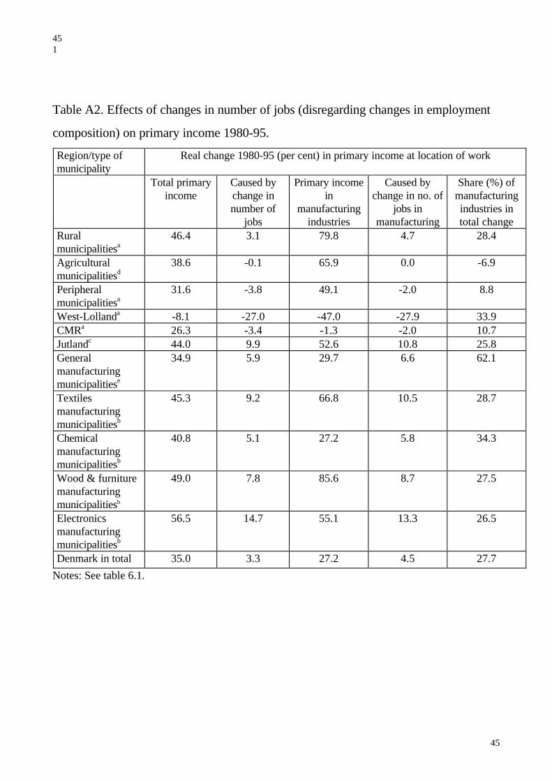
The calculation results from the first decomposition step, the effect of changing the

number of jobs without specialisation (that is, number of employed persons, with no

changes of employment composition) is shown in table A2. For most categories of

municipalities, clearly changes in number of jobs have limited effect on primary

income. This is true for total income as well as manufacturing income. The only

exception is West Lolland, where the collapse of large industrial plants has been

crucial in the negative development of that region.

311

31

It might be noted, though, that the municipalities with specialised manufacturing

industries have done better than other categories, and that growth of manufacturing

employment has contributed markedly (26 to 35 per cent) to growth caused by change

in number of jobs.

When incorporating employment composition in the equation (table A3),

paradoxically, effects on primary income are reduced in most categories. It might have

been expected that people moved from lower paid jobs to higher paid jobs, thereby

raising primary income whenever employment composition changes. It turns out that

the opposite is true. Part of the explanation may be the decline in sunset industries like

shipyards, since jobs in such places have generally been well paid. Persons laid off in

such industries may often have been unable to obtain equally well paid jobs. It might

be said that the loss of primary income seen in table A3 (when compared with A2) is

the price of the loss of competitiveness of such industries. In particular, the loss of jobs

in the manufacturing industries of the CMR more than accounts for the total loss of

primary income in the region, reflecting retrenchments in shipbuilding, newspaper

printing, breweries, and more.

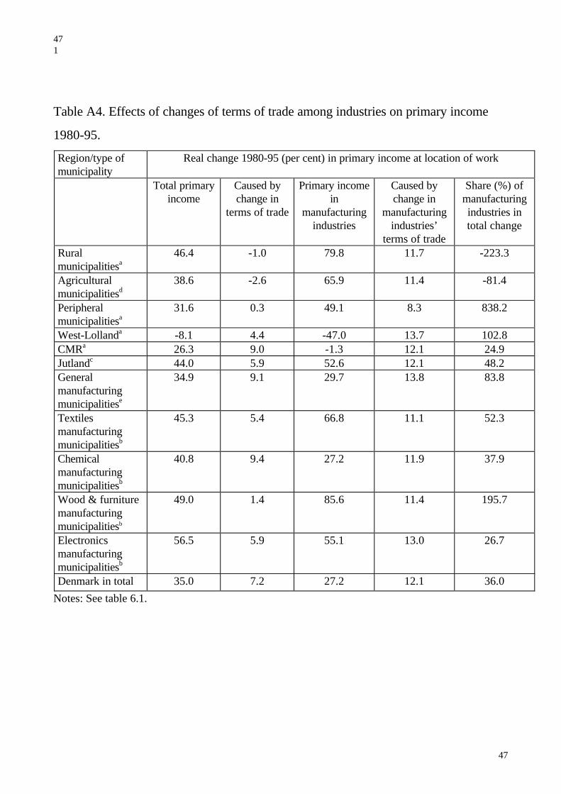
Changes in primary income due to changes in terms of trade among industries are

shown in table A4. A small or negative figure here indicates that a large part of

incomes have been earned in industries with little increase in prices, such as

agriculture. Conversely, for municipalities dominated by industries with rapidly

increasing prices we would expect a high figure. This is exactly what table A4 shows.

In particular, note that the changes caused by manufacturing industries’ terms of trade

are fairly equal in all of the groups. Differences in the change in total primary income,

thus, are primarily due to different intensities of agriculture.

321

32

Changes in primary income related to changes in national labour productivity are

displayed in table A5. Due to data unavailability (see above), national productivity in

manufacturing industries varies very little among the groups. As labour productivity in

all industries and in manufacturing industries happen to have changed identically (30.5

per cent), the effect on total primary income in various groups depends very much on

the shares of manufacturing and agriculture (where productivity has grown more than

in manufacturing industries).

Local labour productivity is measured simply as primary income in municipalities per

person employed. Deviations from the national level indicate a strong or weak

productivity performance compared with the national level. Results are displayed in

table A6. Note that there is a difference for Denmark in total between change caused

by a change in national and local productivity in manufacturing industries. This is not

too surprising, since productivity in 1995 is calculated using employment in 1995,

whereas income change caused by this productivity increase is weighted using

employment in 1980. When all industries are aggregated, differences tend to even out,

but for individual industries and municipalities differences can be substantial.

This section will be concluded with a summary exposition of the results concerning

disposable incomes. We do not have data on disposable income in municipalities of

work (nor, arguably, is such a concept meaningful). Only municipalities of residence

are relevant for this category. In table A7 the results of the decomposition analysis for

each of the thirteen decomposition steps (see tables 5.1 and 5.2) are given for all

industries and for manufacturing industries (where relevant) and for rural and

peripheral municipalities.

331

33

It is seen, in general, that most of the tendencies exposed in the analysis of primary

income are found again in this material, but often reduced to some extent. This is

because changes in primary income, when transformed to disposable income at

municipality of residence, are mitigated in a number of ways.

First, commuting between municipalities help spread increases and decreases of

income among municipalities. Second, transfer incomes such as unemployment

benefits help soften the effects of increasing unemployment and, conversely, dampens

the effect of increasing employment (because unemployment, and related benefits, may

decrease as a result). Third, the so-called fiscal federalism is at work in this context:

Rising primary income will increase taxes, and vice versa.

7. Recent Trends in Manufacturing Industries.

As noted earlier, recent data from the KRNR database seem to change some of the

findings of the last sections. To obtain a perspective for the future, some of the data

are presented in the following. The data invokes the possibility that at least part of the

industrialisation of Jutland in the eighties has in fact represented a postponement of the

inevitable effects of globalisation: That Denmark and most other rich countries are

bound to lose market shares to low wage countries in Asia and elsewhere12. However,

recent data also display some surprises.

12 Note that the recent ”Asian Crisis” does not change this perspective. On the contrary: The crisis has brought alongsubstantial adjustments of currency exchange rates in most of the affected countries, making these even morecompetitive.

341

34

Table A8 shows some patterns of this set of recent data. Data on gross value added

(GVA) as well as employment are given. We see some new trends, but also a

continuation of some of the tendencies that was pointed out by the decomposition

analysis. In this period, the Danish economy has grown fairly well with 15.9 per cent

increase in GVA. Manufacturing industries account for almost one quarter of this.

Employment grew by 4.6 per cent, but here, manufacturing industries has almost no

importance. However, these changes have been very unevenly distributed among

regions and municipality groups. In the following, the most important of the emerging

patterns will be expounded.

Starting with the rural and agricultural municipalities, we see that for all industries,

GVA has grown almost as much as the national average, whereas employment has

stagnated or fallen13. However, this is not due to the performance of manufacturing

industries. On the contrary, GVA and employment in manufacturing industries have

grown more than the country’s average. So the weak development in the general

economy of these municipalities must be ascribed to other industries. Hence, the

hypothesis on above-average growth of manufacturing industries in rural areas is once

again confirmed.

Almost the same pattern is found for peripheral municipalities, only here growth of

GVA in manufacturing is slightly less than the national average. All in all, we find it

fair to say that this evidence does not support the hypothesis that the less favourable

development in peripheral areas is caused by a weak performance of the manufacturing

13 The reduction of employment is noteworthy, since this period is known as one of economic recovery.

351

35

industries. Again, the unfavourable development in these regions must be due to other

industries14.

In West-Lolland, even after 1993 (six years after the closure of Nakskov shipyard) the

development is still gloomy. The lowest GVA growth and the largest fall in

employment among the municipality groups shown in figure A8 is found here.

Employment in manufacturing industries has fallen more than ten per cent, accounting

for almost three fourths of the total decline in employment. However,

GVA in manufacturing has grown almost as much as the national average, implying a

substantial increase in productivity (just as in the period 1980-95, see below).

The trends exposed this far have been fairly similar to those observed in the period

1980-95 for the same regions. So the tendencies observed previously are, by and large,

confirmed by the new data. However, not so when comparing the CMR and Jutland.

From 1993 to 97 GVA growth is higher in the CMR than in Jutland, in particular so

for manufacturing industries. Also, employment has grown faster in the CMR than in

Jutland. However, employment in manufacturing industries has grown slightly in

Jutland, whereas it has fallen a bit in the CMR (although this fall is amply mitigated by

other industries). Such a re-invigoration of manufacturing industries in metropolitan

regions is found in other places in Europe as well (Keeble & Wever 1986).

The developments of manufacturing industries in the CMR and in Jutland represent a

confirmation that some of the industrialisation of Jutland constitutes a postponement of

globalisation. Note, however, that this is not true for rural industrialisation in general

(see above).

14 The ”island periphery” consisting of Bornholm and some other islands is performing much worse than theperiphery in general. But even here, manufacturing industries are doing better than the general economy.

361

36

With so many winners (rural municipalities, the CMR etc.), who are the losers?

Obviously, West-Lolland is one. But also the general manufacturing municipalities, the

“company towns”, have lost out. In these municipalities GVA in manufacturing

industries has not grown at all. And since manufacturing industries are so important in

these places, general GVA growth is far below the national average. Note, however,

that employment in these municipalities has grown a little more than the national

average (also indicating a weak development of labour productivity).

Perhaps the most remarkable fact of the data of table A8 is the substantial difference

between the general manufacturing municipalities and the specialised municipalities.

Where manufacturing GVA has not grown at all in the “company towns”, in the

specialised municipalities it has grown at rates from just below the average (textiles) to

well above it (chemicals, wood and furniture).

Not surprisingly, of the specialised municipalities the textiles manufacturing

municipalities are doing worst. Obviously, this branch of manufacturing is extremely

exposed to international competition from Asian and other low cost countries. Hence,

it is no surprise that employment has fallen ten per cent in manufacturing industries in

these municipalities. One the plus side, however, note that GVA has grown almost as

much as the national average.

For the textiles industries in general, the whole period has been hard times. In the four

years from 1993-97, employment in the textiles industries in the whole country has

declined with more than six thousand jobs or 27 per cent. In their “own”

municipalities, the decline is slightly less, 25.8 per cent, approximately 2800 jobs,

more than four times the net number of job losses in these municipalities (meaning that

371

37

other industries have compensated most of the loss). In the case of the textiles

manufacturing municipalities, it is fair to say that the advance of the period of 1980-95

has constituted a postponement of the effects of globalisation.

In the other specialised municipalities, the development has been much more

benevolent. The most successful group is the chemicals manufacturing municipalities,

where GVA growth in manufacturing industries is almost twice the national average,

and accounts for almost half of the total GVA growth in these municipalities. In the

chemicals manufacturing itself, employment has increased by 1711 jobs, almost as

much as in manufacturing in total (1922 jobs). Even so, the contribution to the total

increase in number of jobs in all industries is modest: More than ten thousand jobs

were generated in these municipalities. Part of the reason is probably that many of

these municipalities are large and have versatile economies.

8. Theories and Evidence. Lessons from the Analyses.

The time has come to review the theories and hypotheses put forth in section 2 in the

light of the evidence given. In so doing, we will condense the data and calculation

results displayed to focus on the essentials.

To sum up, the decomposition analysis of primary incomes show us that a very

substantial relocation of Danish manufacturing industries has taken place from 1980 to

1995. Manufacturing in the rural and peripheral areas has grown more than in the

urban areas. Also, manufacturing in Jutland has grown much more than in the CMR,

where incomes earned in manufacturing industries has actually declined. However,

productivity has increased more than average in some of the unsuccessful regions,

381

38

including West Lolland and the CMR. Further, the developments of general

manufacturing and specialised municipalities suggest that technological spillovers and

labour pooling is important for success of manufacturing industries as a whole,

whereas economies of scale seems less important in the Danish case.

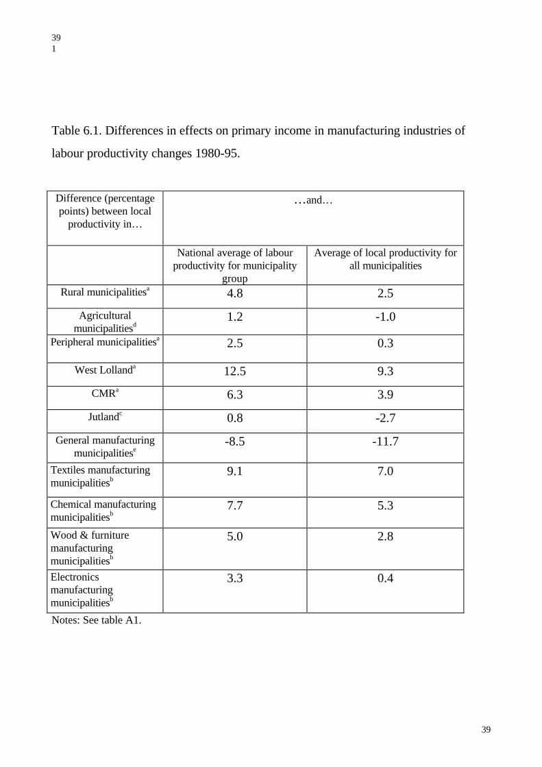
Now we venture to examine productivity growth in the various municipality groups.

More specifically, we will compare effects of national productivity increases and

effects of local deviations from this. This is done by comparing tables A5 and A6, and

including additional evidence from recent data. Results of the comparison of the two

tables are given in table 8.1.

The difference between national average productivity increase and the average of local

productivity increase (see above) poses a question in relation to this: When comparing

results from individual groups of municipalities, should the reference point be average

national productivity (bottom line of table A5), or should it be national average of local

productivity (bottom line of table A6)? As there is no unique answer to this, both

comparisons are given below.

391

39

Table 6.1. Differences in effects on primary income in manufacturing industries of

labour productivity changes 1980-95.

Difference (percentagepoints) between local

productivity in…

…and…

National average of labourproductivity for municipality

group

Average of local productivity forall municipalities

Rural municipalitiesa 4.8 2.5

Agriculturalmunicipalitiesd

1.2 -1.0

Peripheral municipalitiesa 2.5 0.3

West Lollanda 12.5 9.3

CMRa 6.3 3.9

Jutlandc 0.8 -2.7

General manufacturingmunicipalitiese

-8.5 -11.7

Textiles manufacturingmunicipalitiesb

9.1 7.0

Chemical manufacturingmunicipalitiesb

7.7 5.3

Wood & furnituremanufacturingmunicipalitiesb

5.0 2.8

Electronicsmanufacturingmunicipalitiesb

3.3 0.4

Notes: See table A1.

401

40

Table 6.1 contains a lot of noteworthy information. First we note that rural, agricultural

and peripheral municipalities are coping quite nicely when it comes to productivity.

West Lolland has the best productivity record of all the groups.

Comparing the performances of the CMR and Jutland is particularly interesting. As we

suspected, the CMR has had a higher productivity increase than Jutland. This could be

a confirmation of the hypothesis that the development in the respective parts of the

country follows a pattern of exploitation of comparative advantages: In the CMR,

manufacturing industries have increasingly made use of employees with higher

education, and higher salaries, in branches like medicine and electronics. In Jutland

manufacturing firms have taken advantage of the presence of a labour force that has

high work ethics and loyalty towards their firm (Jensen-Butler 1992, see also above,

and Maskell 1992), and who will also accept lower pay (although the difference is not

so large, see above).

The worst performer of the groups when it comes to productivity is the general

manufacturing municipalities. Since these municipalities represent the “dinosaurs” of

Danish manufacturing industries, this is perhaps not too surprising to a Danish

newspaper reader: One large manufacturing firm after the other has been in crisis and

has gone through retrenchments, and worse. The most spectacular case is the closure

of the shipyard in Nakskov in 198715; but note that Nakskov is also part of West

Lolland, which has the highest productivity growth of all groups. So the case of

Nakskov does not explain much. Rather, the period has been bad times for most large

manufacturing plants and for “company towns”.

15 Up till the seventies, Denmark was known as a shipbuilding nation. After closures of shipyards in Elsinore,Aalborg, Nakskov, Copenhagen, Ringkøbing, Svendborg…. this is hardly the case any more. The shipyard inMunkebo (one of the general manufacturing municipalities) seems to be doing well, though.

411

41

By contrast, the specialised manufacturing municipalities do much better. In textiles

and wood and furniture there are no individual firms large enough to dominate income

generation in any municipality. In chemicals and electronics there is a number of large

companies, but few of them dominate local income generation, and only one coincides

with the general manufacturing municipalities (namely Bang & Olufsen, located in

Struer in West Jutland). The lesson seems to be that successful agglomeration is

caused by technological spillovers and labour pooling rather than economies of scale,

at least in the period considered here. In Danish manufacturing industries, Small is

Beautiful, and Large is Lousy.

The relatively low productivity performance of the Jutland manufacturing industries in

this period may constitute a warning: Is the success of manufacturing in this part of the

country only a postponement of the inevitable consequences of globalisation? Are the

Jutland manufacturing firms bound to lose competitiveness to low wage countries in

Asia and elsewhere? Recent evidence, as we have seen, reveal some of the answers.

Notably, this was foreseen by Jensen-Butler (1992, pp. 900-02).

When comparing the evidence from 1993-97 on different groups of manufacturing

municipalities, once again the lesson is that specialisation pays, but size does not. With

the exception of the extremely vulnerable textiles manufacturing municipalities, the

specialised municipality groups fare better than almost any of the other groups. This is

true for GVA and for employment, for manufacturing industries and for all industries.

However, the figures do not confirm the hypothesis that manufacturing industries in

Denmark benefit from economies of scale. This is seen from the fact that the group of

general manufacturing municipalities is among the worst performers of all. As a

consequence, it seems that labour pooling and technological spillovers among firms in

the same industry are responsible for this pattern.

421

42

431

43

10. Concluding remarks.

This essay has aimed to contribute to the knowledge on the consequences of the

changes in the location of manufacturing industries that has been going on in the

eighties and nineties. We have shown to what extent the very substantial relocation of

manufacturing industries have contributed to the growth of primary incomes and

disposable incomes in rural, peripheral and many other regions and types of

municipalities.

Early in the essay we expressed some hypotheses for discussion. We have found

evidence on each of them:

• • The hypothesis on the role of manufacturing industries in income growth in rural

areas is confirmed by the evidence, but it cannot be confirmed that manufacturing

industries are instrumental in the decline of peripheral regions.

• To some extent the hypothesis on comparative advantages is supported: Growth of

manufacturing industries in Jutland is, among other things, caused by the presence

of a loyal and compliant work force (Jensen-Butler 1992, Illeris 1986), while in the

CMR, manufacturing industries have taken advantage of the presence of a large

labour force with higher education. Also to some extent, our suspicions on part of

the Jutland industrialisation are confirmed: In the textiles industries, above all,

employment has recently declined substantially.

• Successful local concentration of manufacturing production has taken place in the

specialised municipalities, indicating that technological spillovers and labour

pooling are important in this context. However, it is not confirmed that economies

of scale is important for manufacturing growth.

441

44

• • Appendix 1. Tables.

Table A1. Major trends in the development of manufacturing industries in various

parts of the country:

Region/type ofmunicipality

Real change 1980-95 (per cent) at location of work in

Totalemployment

Total primaryincome

Employment inmanufacturing ind.

Primary income inmanufacturing ind.

Ruralmunicipalitiesa

2.9 46.4 32.0 79.8


-1.4 38.6 25.7 65.9

Peripheralmunicipalitiesa

-4.6 31.6 10.2 49.1

West-Lollanda -27.0 -8.1 -60.5 -47.0CMRa -2.5 26.3 -27.0 -1.3Jutlandc 9.8 44.0 16.7 52.6Generalmanufacturingmunicipalitiese

7.0 34.9 7.7 29.7

Textilesmanufacturingmunicipalitiesb

9.2 45.3 18.3 66.8

Chemicalmanufacturingmunicipalitiesb

5.0 40.8 -7.6 27.2


7.4 49.0 37.4 85.6


15.0 56.5 19.2 55.1

Denmark in total 3.8 35.0 -2.4 27.2

Notes: A complete list of municipalities in the categories listed is available from the authors. Thecategories are defined as follows.a) See appendix 2.b) Location factor 4 used on gross value added in 1995 in each of the industries.c) Comprises all of the seven counties of Jutland, including surrounding islands.d) Location factor 4 used on primary income in 1980.e) Location factor 2 used on primary income in 1980.

451

45

Table A2. Effects of changes in number of jobs (disregarding changes in employment

composition) on primary income 1980-95.


Real change 1980-95 (per cent) in primary income at location of work

Total primaryincome

Caused bychange innumber of

jobs

Primary incomein

manufacturingindustries

Caused bychange in no. of

jobs inmanufacturing

Share (%) ofmanufacturingindustries intotal change


46.4 3.1 79.8 4.7 28.4


38.6 -0.1 65.9 0.0 -6.9


31.6 -3.8 49.1 -2.0 8.8

West-Lollanda -8.1 -27.0 -47.0 -27.9 33.9CMRa 26.3 -3.4 -1.3 -2.0 10.7Jutlandc 44.0 9.9 52.6 10.8 25.8Generalmanufacturingmunicipalitiese

34.9 5.9 29.7 6.6 62.1


45.3 9.2 66.8 10.5 28.7


40.8 5.1 27.2 5.8 34.3


49.0 7.8 85.6 8.7 27.5


56.5 14.7 55.1 13.3 26.5

Denmark in total 35.0 3.3 27.2 4.5 27.7

Notes: See table 6.1.

461

46

Table A3. Effects of employment changes, incorporating changes in employment

composition, on primary income 1980-95.



Total primaryincome

Caused bychange in totalemployment

Primary incomein


Caused bychange in

manufacturingemployment



46.4 3.6 79.8 31.1 162.8


38.6 -0.8 65.9 26.3 -597.5


31.6 -6.8 49.1 8.3 -20.4

West-Lollanda -8.1 -28.6 -47.0 -61.4 70.6CMRa 26.3 -4.8 -1.3 -28.6 110.5Jutlandc 44.0 8.0 52.6 14.3 42.4Generalmanufacturingmunicipalitiese

34.9 0.8 29.7 -3.7 -244.3


45.3 7.7 66.8 19.2 62.5


40.8 4.5 27.2 -8.4 -56.0


49.0 8.0 85.6 38.4 118.7


56.5 14.1 55.1 14.3 29.5

Denmark in total 35.0 1.2 27.2 -5.2 -107.1


471

47

Table A4. Effects of changes of terms of trade among industries on primary income

1980-95.



Total primaryincome

Caused bychange in

terms of trade

Primary incomein


Caused bychange in

manufacturingindustries’

terms of trade



46.4 -1.0 79.8 11.7 -223.3


38.6 -2.6 65.9 11.4 -81.4


31.6 0.3 49.1 8.3 838.2

West-Lollanda -8.1 4.4 -47.0 13.7 102.8CMRa 26.3 9.0 -1.3 12.1 24.9Jutlandc 44.0 5.9 52.6 12.1 48.2Generalmanufacturingmunicipalitiese

34.9 9.1 29.7 13.8 83.8


45.3 5.4 66.8 11.1 52.3


40.8 9.4 27.2 11.9 37.9


49.0 1.4 85.6 11.4 195.7


56.5 5.9 55.1 13.0 26.7

Denmark in total 35.0 7.2 27.2 12.1 36.0


481

48

Table A5. Effects of national labour productivity changes (incorporating terms of trade

changes) on primary income 1980-95.



Total primaryincome

Caused bychange in

national labourproductivity

Primary incomein


Caused bychange in nat.

labourproductivity in

manuf. ind.



46.6 38.0 79.8 30.7 15.3


38.6 38.8 65.9 30.8 14.6


31.6 35.6 49.1 30.8 14.2


34.9 31.6 29.7 29.8 52.1


45.3 32.0 66.8 30.9 24.4


40.8 29.7 27.2 30.6 30.9


49.0 35.7 85.6 30.8 21.3


56.5 32.8 55.1 30.1 26.7

Denmark in total 35.0 30.5 27.2 30.5 21.5


491

49

Table A6. Effects of local labour productivity changes (incorporating changes in terms

of trade) on primary income 1980-95.



Total primaryincome

Caused bychange in totalemployment

Primary incomein


Caused bychange in

manufacturingemployment



46.6 39.0 79.8 35.5 17.3


38.6 38.8 65.9 32.0 15.1


31.6 35.7 49.1 33.3 15.5


34.9 25.3 29.7 21.3 46.6


45.3 32.2 66.8 40.0 31.3


40.8 33.4 27.2 38.3 34.3


49.0 36.6 85.6 35.8 24.2


56.5 34.1 55.1 33.4 28.5

Denmark in total 35.0 30.5 27.2 33.0 23.2


501

50

Table A7. Decomposition of changes of disposable income. Per Cent Change.

Decomposition step:Change caused by… ↓

All industries Manufacturing industries

Rurala Peripherala Rurala Peripherala

1 Change in numberof jobs

1.4 -0.2 * *

2 Change inemployment,includingcomposition

-0.1 -2.6 0.6 0.2

3 Change in relativeprices

2.3 1.7 0.4 0.2

4 Change in nationalproductivity

26.3 25.0 5.3 4.3

5 Change in localproductivity

26.1 24.4 5.2 4.6

6 Change inpopulation size andcomposition

4.0 0.0 * *

7 Change in labourforce activity rate

-1.2 -2.6 * *

8 Change incommuting pattern

-0.0 -0.4 0.5 0.2

9 Change ineducationalcomposition ofpopulation

0.6 0.5 * *

10 Change in transferrates

7.3 8.0 * *

11 Change in transferstructure

8.0 8.0 * *

12 Change in tax rates -6.5 -5.8 * *

13 Change in taxstructure

-1.1 -1.4 * *

Total change indisposable income

33.7 26.4 * *

Notes: See table A1.*: Not relevant.

511

51

Table A8. Growth of gross value added (GVA) and employment in all industries andmanufacturing industries 1993-97.

Real change 1993-97 (per cent).


Grossvalue

added, allindustries

Gross valueadded,


Share ofmanufacturingindustries in

change

Employmentall industries

Employ-ment, ma-

nufacturingindustries

Share ofmanufactu-

ringindustriesin change


14.7 28.9 35.8 0.0 5.4 2676.2


15.6 30.1 33.2 -1.5 2.3 -30.0


10.7 18.6 27.8 0 5.3 f)

West-Lollanda 8.9 21.0 40.6 -1.9 -10.7 74.8CMRa 17.2 31.2 21.0 6.0 -3.9 -8.2Jutlandc 14.2 19.3 29.4 4.1 2.7 14.2Generalmanufacturingmunicipalitiese

10.1 0.0 0.1 4.2 1.8 20.4


17.4 22.3 34.0 -0.8 -9.2 336.1


24.2 41.5 44.8 7.3 6.4 19.1


17.7 30.2 42.7 1.0 4.3 110.6


23.4 27.6 32.1 4.8 2.9 15.6

Denmark in total 15.9 23.3 24.6 4.6 0.6 2.3

Notes a-e: See table 6.1.

f: Zero denominator!

521

52

Appendix 2: Definitions of municipality groups and regions.

Rural municipalities: Municipalities with no towns larger than 3000 inhabitants as ofJan. 1, 1984.

Peripheral municipalities: Municipalities on Bornholm and smaller islands exceptFanø plus rural municipalities with- a distance of more than 40 kilometres to the closest strong geographical centre in

turn defined as having a commuting intensity of more than 2.0 and more than 40000jobs as of Jan. 1 1984; and

- a distance of more than 30 kilometres to the closest geographical centre, defined ashaving either more than 20000 jobs or more than 10000 jobs and a commutingintensity of more than 2.0.

West-Lolland comprises the municipalities Højreby, Nakskov, Ravnsborg andRudbjerg.

The CMR consists of the Municipalities of Copenhagen City and Frederiksberg and thecounties of Copenhagen, Frederiksborg and Roskilde.

531

53

References.

Andersen, Anne Kaag (1998): Decomposition of the Change of the Amount ofCommuting in Denmark 1980-1995. AKF memo, Copenhagen.

Atalik, Gündüz and Levent, Tüzin Baycan (1998): An Interpretation of the Impact ofRegional Science in Terms of Philosophy of Science. Papers in Regional Science(77:4), October 1998, pp. 329-46.

Beckmann, M.J. and Thisse, J.F. (1986): The Location of Production Activities.Chapter 2 in Nijkamp, P (ed.): Handbook of Regional and Urban Economics. Vol 1:Regional Economics. North-Holland: Amsterdam et al.

Filges, Trine; Lehrmann Rasmussen, Jens; Madsen, Bjarne; Jensen-Butler, Chris(1999): LINE – a Model of 275 Danish Municipalities. Forthcoming in Structures andProspects of Nordic Regional Economies.

Harris, J.R. and Todaro, Michael P. (1970): Migration, Unemployment, andDevelopment. A Two-Sector Analysis. American Economic Review 60, pp. 126-42.

Hart, Mark and Gudgin, Graham (1994): Spatial Variations in New Firm Formation inthe Republic of Ireland. Regional Studies (28:4), pp. 367-80.

Illeris, Sven (1986): New firm creation in Denmark: the importance of the culturalbackground. Chapter 7 in Keeble, David & Wever, Egbert (eds.): New Firms andRegional Development in Europe. Croom Helm, London et al.

Jensen, Torben Pilegaard; Maskell, Peter; Arnberg, Søren; Hansen, Morten Bjørn;Ranis, Troels (1997): Erhvervslokalisering og vækst [Business Location and Growth.With English summary]. AKF rapport, Copenhagen.

Jensen-Butler, Chris (1992): Rural Industrialisation in Denmark and the Role ofPublic Policy. Urban Studies (29:6), pp. 881-904.

Jensen-Butler, Chris; Madsen, Bjarne; Caspersen, Søren (1999): Rural areas in crisis?The role of the welfare state in income creation, the case of Denmark. Unpublishedmemo, AKF, Copenhagen.

Jorgenson, Dale W. (1967): Surplus Agricultural Labor and the Development of aDual Economy. Oxford Economic Papers.

541

54

Keeble, David & Wever, Egbert (1986): Introduction. Chapter 1 in Keeble, David &Wever, Egbert (eds.): New Firms and Regional Development in Europe. Croom Helm,London et al.

Keeble, David & Kelly, Tomythy (1986): New firms and high-technology industry inthe United Kingdom: the case of computer electronics. Chapter 4 in Keeble, David &Wever, Egbert (eds.): New Firms and Regional Development in Europe. Croom Helm,London et al.

Krugman, Paul (1991): Geography and Trade. Leuven University Press & The MITPress, Leuven et al.

Krugman, Paul (1995): Development, Geography, and Economic Theory. The MITPress, Cambridge, Massachusetts et al.

Lehrmann Rasmussen, Jens (1994): The Choice of Development Strategy in a DualEconomy. Ph.D.-thesis, Aarhus School of Business, Series K no. 30.

Lewis, W. Arthur (1954): Economic Development with Unlimited Supplies of Labour.The Manchester School.

Madsen, Bjarne; Jensen-Butler, Chris; Dam, Poul Uffe (1998): The LINE Model.Unpublished, AKF, Copenhagen.

Madsen, Bjarne; Jensen-Butler, Chris; Filges, Trine; Lehrmann Rasmussen, Jens(1999): Local National Accounts for Denmark: The SAM Approach. Forthcoming inStructures and Prospects of Nordic Regional Economies.

Malmberg, Anders and Maskell, Peter (1997): Towards an Explanation of RegionalSpecialization and Industry Agglomeration. European Planning Studies (5:1), pp. 25-41.

Maskell, Peter (1992): Nyetableringer i Industrien [New firm formation andstructural change in Danish manufacturing industry. With English summary].Handelshøjskolens Forlag et al.: Copenhagen.

O’Farrell, P.N. (1986): The nature of new firms in Ireland: empirical evidence andpolicy implications. Chapter 8 in Keeble, David & Wever, Egbert (eds.): New Firmsand Regional Development in Europe. Croom Helm, London et al.

551

55

Wier, Mette (1998): Sources of Changes in Emissions from Energy: A StructuralDecomposition Analysis. Economic Systems Research (10:2) June 1998, pp.

changing patterns of manufacturing growth … · we will try to trace effects of the changing...

Documents