Chaos and Dynamical Systemsby Megan Richards

Abstract: In this paper, we will discuss the notion of chaos. We will start by introducing certain mathematical con-

cepts needed in the understanding of chaos, such as iterates of functions and stable and unstable fixed points. We will

discuss the graphical analysis of an orbit and show a couple examples of an orbit diagram. We will briefly show how

the Lyapunov exponent can be found and used to determine whether a system is chaotic and if so where it is chaotic.

Then we will begin discussing the baker map, which this paper focuses on the most. In particular, we will discuss the

values at which the baker map exhibits chaotic behavior and why it is chaotic at those values. This has been focused on

because, while it can be easy for someone to pick up a book and read about chaos, it may not be so easy to research the

baker map and find the values at which it is chaotic and why. Finally, we will look at an example of a known chaotic

system – the double-pendulum. We will use a computer program to model the behavior of the pendulum and observe

how it is sensitive to initial conditions. In this paper, we will assume that the reader has a mathematical background

up to the calculus level and can understand certain proof techniques, such as a proof by induction or by contradiction.

Introduction

Chaos is a word we all know usually meaning a lack of order or predictability. Most people might associate

the “butterfly effect” with the notion of chaos. This “butterfly effect” describes how a butterfly flapping its

wings in some part of the world might be largely responsible for a huge storm in another part of the world

several weeks later, because of the weather’s extreme sensitivity to initial conditions.

The weather is indeed one example of a chaotic system. A weather reporter might make nearly identical

forecasts for a city in Europe as for a city in the United States, meaning that the initial conditions of the

system are quite similar, while by the next week the weather patterns are completely different. Because of

this sensitive dependence on initial conditions, weather forecasters have a very difficult time predicting the

weather far in advance.

Another example of chaos is the double pendulum, and later we will use a computer program to model

the motion of a double pendulum. We will place the double pendulum at a certain initial point and again

1

at another initial point just slightly different than the first to observe how the resulting motion will be very

different.

What makes certain systems chaotic? Chaos describes the behavior of a system that is highly sensitive to

initial conditions. Chaotic systems are not predictable over a long period of time and are typically associated

with fractal structures.

Understanding chaos will help us understand why some systems exhibit seemingly erratic and random

behavior yet are still deterministic systems (that is, systems determined by their initial conditions). It will

show us why chaos is not complete disorder, but rather is associated with a geometrical structure.

Understanding chaos is somewhat complicated, so we first need to be able to understand certain math-

ematical concepts and the instability and stability of non-chaotic systems. Hence, this paper will begin by

explaining iterates of functions, unstable and stable fixed points, and some examples of maps and orbit dia-

grams. We will then move on to discuss the baker map and at which points the baker map exhibits chaotic

behavior. Finally we will show the motion of a double-pendulum using a computer program.

Maps

First we will look at the iterates of functions. Suppose that f is a function and x0 is an element of the

domain of f . The iterates of x0 will consist of x0, f(x0), f(f(x0)), f(f(f(x0))), .... These iterates together

are called the orbit of x0. Note we can write xn+1 = f(xn), which we often refer to as a map, so that the

orbit of x becomes x0, x1, x2, x3, .....

As an example, consider the map xn+1 = cos(xn), and let x0 = 0.5. To find the iterates of x0, we enter

0.5 into a calculator. Then we enter cos(Ans) repeatedly. The first iterate of x0 for f is x1 = f(x0) =

.8775825619. The second iterate is x2 = f(f(x0)) = .6390124942, and so on. The orbit of x0 will start

looking like

0.5, 0.8775825619, 0.6390124942, 0.8026851007, 0.6947780268, ...

If we press cos(Ans) enough times, we end up repeatedly getting the calculator to spit out the number

.7390851332. This number describes the value of x for which x = cos(x). This value of x is called a fixed

point of f . In general, if we have a function f and a number c in the domain of f , c is a fixed point of f if

2

f(c) = c. We can visualize this graphically by plotting the line y = x with the graph of f and finding where

they intersect.

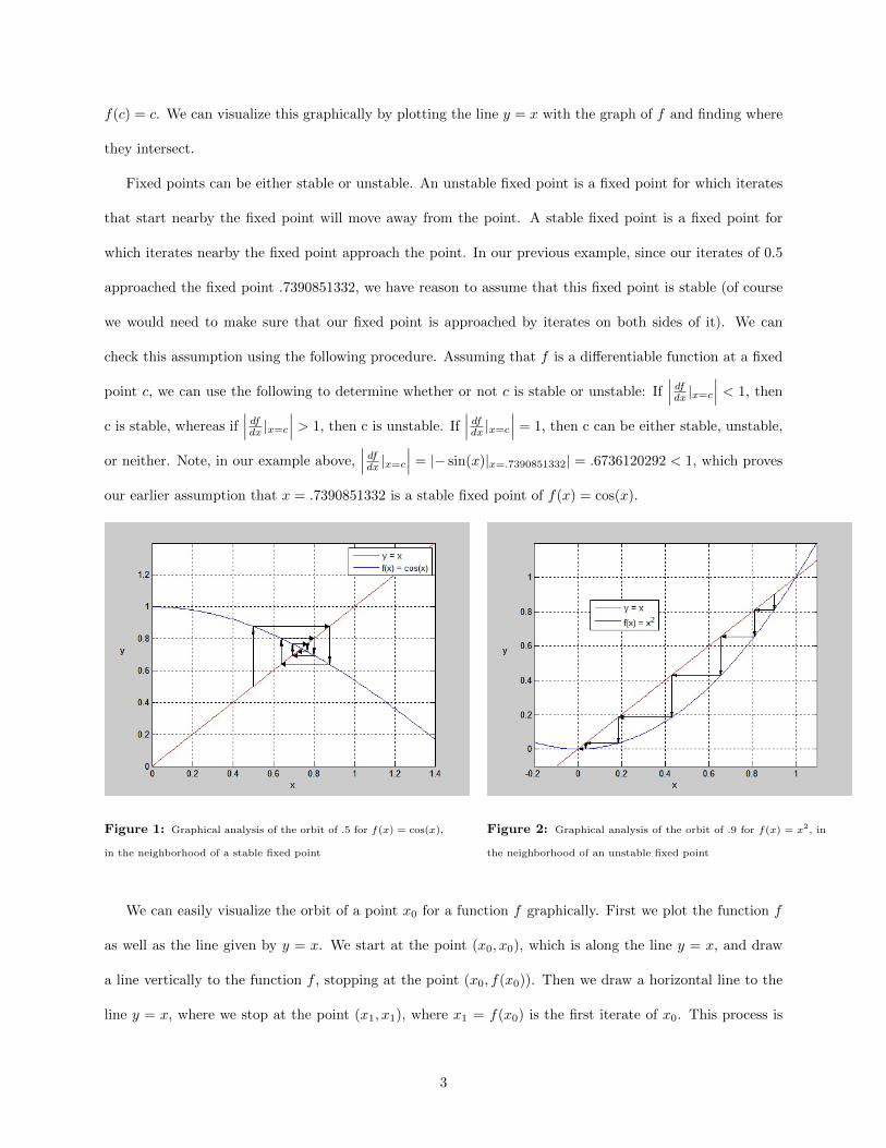
Fixed points can be either stable or unstable. An unstable fixed point is a fixed point for which iterates

that start nearby the fixed point will move away from the point. A stable fixed point is a fixed point for

which iterates nearby the fixed point approach the point. In our previous example, since our iterates of 0.5

approached the fixed point .7390851332, we have reason to assume that this fixed point is stable (of course

we would need to make sure that our fixed point is approached by iterates on both sides of it). We can

check this assumption using the following procedure. Assuming that f is a differentiable function at a fixed

point c, we can use the following to determine whether or not c is stable or unstable: If∣∣∣ dfdx |x=c

∣∣∣ < 1, then

c is stable, whereas if∣∣∣ dfdx |x=c

∣∣∣ > 1, then c is unstable. If∣∣∣ dfdx |x=c

∣∣∣ = 1, then c can be either stable, unstable,

or neither. Note, in our example above,∣∣∣ dfdx |x=c

∣∣∣ = |− sin(x)|x=.7390851332| = .6736120292 < 1, which proves

our earlier assumption that x = .7390851332 is a stable fixed point of f(x) = cos(x).

Figure 1: Graphical analysis of the orbit of .5 for f(x) = cos(x),

in the neighborhood of a stable fixed point

Figure 2: Graphical analysis of the orbit of .9 for f(x) = x2, in

the neighborhood of an unstable fixed point

We can easily visualize the orbit of a point x0 for a function f graphically. First we plot the function f

as well as the line given by y = x. We start at the point (x0, x0), which is along the line y = x, and draw

a line vertically to the function f , stopping at the point (x0, f(x0)). Then we draw a horizontal line to the

line y = x, where we stop at the point (x1, x1), where x1 = f(x0) is the first iterate of x0. This process is

3

then repeated. The graphical interpretation for the iterates of x0 = .5 for f(x) = cos(x) is given in Figure

1. (Note the Matlab codes used to produce each figure in this paper are given in the Appendix.) Remember

that these iterates converged to the stable fixed point x = .7390851332. We can also see this graphically in

the figure.

Note that for unstable fixed points, iterates will diverge from the fixed point, which can also be seen

graphically. Consider the graphical analysis of the orbit of x0 = .9 for the function f(x) = x2 shown in

Figure 2. First, note that 0 and 1 are fixed points for f since f(1) = 12 = 1 and f(0) = 02 = 0. Note 1 is

unstable since∣∣∣ dfdx |x=1

∣∣∣ =∣∣ ddx (x2)|x=1

∣∣ = |2x|x=1| = 2 > 1, while 0 is stable since∣∣∣ dfdx |x=0

∣∣∣ = |2x|x=0| = 0 < 1.

Thus, iterates of x0 = .9 will move away from the unstable fixed point at 1 and converge to the stable fixed

point at 0.

Now consider iterates of x0 = 13 for the function f(x) = 4x − 4x2. The orbit of 1

3 will begin looking

like {0.333333 · · · , 0.888888 · · · , 0.395061 · · · , 0.9555951 · · · , ...}. We might be expecting these iterates to

converge to a fixed point, as they did with f(x) = cos(x). However, this turns out not to be the case. It

turns out that the iterates are numbers in the interval (0, 1) that have no predictable pattern. This is an

example of a function that exhibits chaos.

Suppose f is a function and x0 is in the domain of f . Then if xn = x0 and if x0, x1, x2, ..., xn−1 are distinct,

we say that x0 has period n. Note if x0 has period n, then the orbit of x0 is given by {x0, x1, x2, ..., xn−1}.

This orbit is called a periodic orbit or an n-cycle. Note that if a point has period 1, it is a fixed point.

A periodic point is a value x for which some iterate is again x. For instance, if we consider the function

f(x) = x2 − 1, the orbit of x0 = −1 is given by −1, 0,−1, 0,−1, ... . Note f(f(x0)) = −1, and so −1 is a

periodic point. In fact, {−1, 0} forms a 2-cycle since f(−1) = 0 and f(f(−1)) = f(0) = −1.

Now consider the map xn+1 = r cos(xn), where r is a real number. To see how this map behaves for

all values of r at once, we plot what is known as an orbit diagram, shown in Figure 3. The darkened

patches represent the areas where the iterates do not converge to a fixed point, but spread out from (r,−r).

It is important to note that this spreading out does not indicate chaos – rather it is the sensitivity to

initial conditions that determines whether or not a system is chaotic. However, in this case sensitivity to

initial conditions does occur in these darkened areas, and so they show the values of r for which the map

4

Figure 3: Orbit diagram for xn+1 = r cosxn

xn+1 = r cos(xn) is exhibiting chaotic behavior.

A function that is parametrized, such as f(x) = r cos(x), is said to have a bifurcation at a point r0 if the

type (stable or unstable) or number of periodic points change at that point. This point r0 is then known as

a bifurcation point for the function f . Thus, as can be seen from the plot in Figure 3, a bifurcation exists

around r0 = −1.3 since at that point our 1-cycle changes to a 2-cycle. This is known as a period-doubling

bifurcation. In general, a period doubling bifurcation is a bifurcation where an n-cycle gives rise to a 2n-cycle.

Period-doubling is a common route to chaos.

The Lyapunov Exponent

The Lyapunov exponent determines whether or not a system is chaotic. The Lyapunov exponent for the

orbit of a function f starting at x0 is given by

λ = limn→∞

{1

n

n−1∑i=0

ln |f ′(xi)|}.

If λ > 0 we have chaotic dynamics. Otherwise, we have a non-chaotic situation. Calculating the Lyapunov

exponent numerically is fairly simple. In general, the Lyapunov exponent is hard to find analytically, but

we will calculate it for a simple example.

Consider the tent map given by

f(x) =

{rx 0 ≤ x ≤ 0.5

r − rx 0.5 ≤ x ≤ 1

5

for 0 ≤ r ≤ 2 and 0 ≤ x ≤ 1.

The derivative of f is then

f ′(x) =

{r 0 ≤ x ≤ 0.5

−r 0.5 ≤ x ≤ 1

The Lyapunov exponent is given by

λ = limn→∞

{1

n

n−1∑i=0

ln |f ′(xi)|}

= limn→∞

{1

n

n−1∑i=0

ln |±r|}

= limn→∞

{1

nln |r|n

}= ln |r| .

Thus, since λ > 0 when |r| > 1, and λ ≤ 0 when 0 < |r| ≤ 1, we get chaos when |r| > 1 and order when

0 < |r| ≤ 1.

Figure 4 shows a plot of the Lyapunov exponent as a function of r for the tent map, while Figure 5 shows

the orbit diagram for the tent map.

Figure 4: Liapunov exponent for the tent map Figure 5: Orbit diagram for the tent map

Note that from the plot of the Lyapunov exponent, we can see that λ > 0 when r > 1, as we found

above. As can be seen in Figure 5, chaotic behavior starts occurring at r = 1, which agrees with the plot

in Figure 4. We also note from the diagram that as r increases the chaotic behavior for the iterates of the

corresponding tent functions is also increasing.

6

The Baker Map

One Dimensional Baker Function:

Let us first introduce a version of the one-dimensional baker function B1, given by

B1 =

{2x 0 ≤ x ≤ 0.5

2x− 1 0.5 < x ≤ 1

First we will show that B1 is extremely sensitive to initial conditions. Let us find some iterates of

23 = 0.6666 · · · and 0.667 to see if they are much different.

iterates 1 2 3 4 5 6 7 8 9 10

23

13

23

13

23

13

23

13

23

13

23

0.667 0.334 0.668 0.336 0.672 0.344 0.688 0.376 0.752 0.504 0.008

Note that the tenth iterates of 23 and 0.667 are, respectively, 2

3 and 0.008, which differ by over 0.6. Thus, even

though we started with two numbers fairly close together, the tenth iterates of those numbers are already

quite far apart. Hence, we cannot relate the higher iterates of 0.667 to the corresponding iterates of 23 . If

we were to experiment further, we would find that choosing a different pair of numbers close together will

exhibit similar behavior.

Two Dimensional Baker Map:

Now, consider the two-dimensional baker map, given by

B(xn, yn) =

{(cxn, 2yn) 0 ≤ yn ≤ 0.5

(1 + c(xn − 1), 2yn − 1) 0.5 < yn ≤ 1

where 0 < c <1

2

First, note that, setting B(x0, y0) = (x0, y0), we obtain two fixed points, namely (0, 0) and (1, 1). Thus,

the points (0, 0) and (1, 1) remain unchanged under the mapping of B. Other points move differently

depending on if they are above or below the line yn = 12 .

7

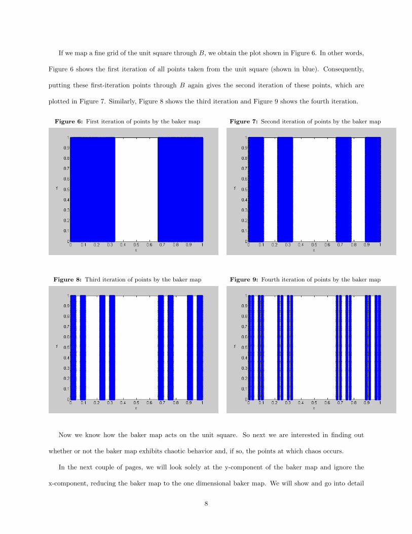
If we map a fine grid of the unit square through B, we obtain the plot shown in Figure 6. In other words,

Figure 6 shows the first iteration of all points taken from the unit square (shown in blue). Consequently,

putting these first-iteration points through B again gives the second iteration of these points, which are

plotted in Figure 7. Similarly, Figure 8 shows the third iteration and Figure 9 shows the fourth iteration.

Figure 6: First iteration of points by the baker map Figure 7: Second iteration of points by the baker map

Figure 8: Third iteration of points by the baker map Figure 9: Fourth iteration of points by the baker map

Now we know how the baker map acts on the unit square. So next we are interested in finding out

whether or not the baker map exhibits chaotic behavior and, if so, the points at which chaos occurs.

In the next couple of pages, we will look solely at the y-component of the baker map and ignore the

x-component, reducing the baker map to the one dimensional baker map. We will show and go into detail

8

about what happens if y0 is rational and conclude that in this case the iterations of y0 repeat. Then we will

show that if y0 is irrational, then the baker map is chaotic. Finally, we will show that chaos in the baker

map actually does not depend on the initial x-value but rather only on the initial y-value.

So, now we will prove that if y0 is a rational number, the iterations of y0 will eventually repeat, which

will result in a non-chaotic situation. More specifically, if y0 = ab , where a, b ∈ Z (so y0 is rational), then y0

will have at most b iterations before an iteration is repeated, or, in other words, y0 or an iteration of y0 will

have at most period b.

Choose y0 = ab , where a, b ∈ Z and 0 < y0 ≤ 1. Then a ≤ b. If y0 ≤ 0.5, then y1 = 2y0 = 2a

b . If y0 > 0.5,

then y1 = 2y0 − 1 = 2ab − 1 = 2a−b

b . Note in both cases the numerator is an integer and the denominator

is b. I can repeat this process and the numerator will still be an integer, while the denominator will still be

the integer b. Since the numerator is an integer and is less than or equal to b, we only have b choices for

the numerator. Thus, we will have at most b iterations of y0 before the iterations begin to repeat. The first

iteration that will be repeated will be either y0 (if the denominator of y0 is not divisible by 2) or an iteration

of y0 (if the denominator is divisible by 2). The previous statement was a bit of a claim to make. Let us

prove this.

Our method of proof will be to introduce a function γ which mimics the baker function when y0 is a

rational number between 0 and 1 whose denominator b is a fixed number that is not divisible by 2. We will

show that γ is injective and hence show that if b is not divisible by 2, then y0 will be repeated in a later

iterate.

Let γb(a) = bB(ab ), where 0 < a < b and b is an integer not divisible by 2. Note we can use our γ function

to represent the numerator values in our iterations of y0 = ab when a and b are integers and b is not divisible

by 2. Since in each iteration the denominator b does not change, we can let y0 = a0b , y1 = a1

b , and so on.

Then we can represent our iterations {y0, y1, y2, ...} as {a0b ,a1b ,

a2b , ..., }. Thus, by0 = a0, by1 = a1, and so on.

So, for instance, γb(a0) = bB(a0b ) = bB(y0) = by1 = a1. Similarly, we have that γb(a1) = bB(a1b ) = by2 = a2,

and so on.

9

Claim 1: The function γ is injective.

Proof. Let a1, a2 ∈ Z. Suppose γb(a1) = γb(a2). We consider the three possible cases and show in each case

a1 = a2.

Case 1: a1, a2 ≤ b2 . Note a1

b ,a2b ≤

12 . Since γb(a1) = γb(a2), we get bB(a1b ) = bB(a2b ). So b 2a1

b = b 2a2b .

Simplifying, we get a1 = a2. Thus, γ is injective.

Case 2: a1, a2 >b2 . Note a1

b ,a2b > 1

2 . Since γb(a1) = γb(a2), we get bB(a1b ) = bB(a2b ). So b 2a1−bb =

b 2a2−bb . Simplifying, we get a1 = a2. Thus, γ is injective.

Case 3: a1 ≤ b2 and a2 >

b2 . Note a1

b ≤12 and a2

b > 12 . Since γb(a1) = γb(a2), we get bB(a1b ) = bB(a2b ).

So b 2a1b = b 2a2−b

b . So 2(a2 − a1) = b, a contradiction since b is not divisible by 2.

Hence, we have proven that γ is injective.

Claim 2: If y0 = ab when a and b are integers and b is not divisible by 2, then y0 will be repeated in a later

iterate.

Proof. Suppose y0 = a0b where b is not divisible by 2, and suppose, for the sake of contradiction, that y0 does

not become repeated later, but that another iterate yi is the first iterate repeated later, where i ≥ 1. Let

yk = yi, where k > i. Then γb(ai−1) = ai = ak = γ(ak−1). Since γ is injective, ai−1 = ak−1, a contradiction

since ai was the first iterate repeated.

Claim 3: Let y0 be in lowest terms. If y0 = ab , where a, b ∈ Z and b is divisible by 2, then y0 will not be

repeated but rather an iterate of y0 will be repeated.

Proof. Suppose y0 = ab , where a, b ∈ Z and b is divisible by 2. Then we can write b = 2m for some m ∈ Z.

Thus, y0 = a2m . If y0 ≤ 0.5, then y1 = 2y0 = a

m . If y0 > 0.5, then y1 = 2y0 − 1 = am − 1 = a−m

m . In

both cases, the denominator reduces to m. If m is again divisible by 2, we repeat the process until we have

an iterate where the denominator is no longer divisible by 2. Let us call this iterate yi. Then, since the

denominator of yi is no longer divisible by 2 and we still have an integer in the numerator, by our previous

proof, yi is the first iterate that will be repeated later. Hence, our inital y0 will not be repeated.

Now let us look at some examples.

10

Suppose y0 = 19 . We expect, since 9 is not divisible by 2, that y0 should be repeated later in at most

nine iterations. As can be seen in the iterates of y0 shown below, we are correct.

iterates y1 y2 y3 y4 y5 y6

19

29

49

89

79

59

19

Note that the 6th iteration returns y0 and so y0 = 19 has period 6. So here we have a non-chaotic situation.

See Figure 10 for a plot of the iterations of (x0, y0) = ( 12 ,

19 ).

Figure 10: Iterations of (x0, y0) = ( 12, 19): a non-chaotic orbit

Now suppose y0 = 310 . In this case the denominator is divisible by 2, and this causes the fraction to be

reduced in the second iterate. The initial value y0 is therefore never repeated, but the first iterate of y0,

namely y1, is repeated. The iterates of y0 are shown below.

iterates y1 y2 y3 y4 y5

310

35

15

25

45

35

Note y5 = y1, and so y1 has period 4. The baker map thus repeatedly spits out the values of y1 through

11

y4 for the y-values and so in this case exhibits non-chaotic behavior.

We have shown that we will get a non-chaotic situation if y0 is rational and have shown a couple examples

of this. So what happens if y0 is irrational? Let us look at when y0 =√

22 . The table below shows the iterations

of this value of y0 up to 24 iterations.

iterates y1 y2 y3 y4 y5 y6 y7 y8

√2

2 0.414214 0.828427 0.656854 0.313708 0.627417 0.254834 0.509668 0.019336

iterates y9 y10 y11 y12 y13 y14 y15 y16

√2

2 0.038672 0.077344 0.154688 0.309376 0.618751 0.237503 0.475005 0.950012

iterates y17 y18 y19 y20 y21 y22 y23 y24

√2

2 0.900024 0.800047 0.600095 0.200189 0.400379 0.800758 0.601516 0.203031

To see how the baker function is sensitive to initial conditions, we will also plot a table of the iterations of

y0 =√

22 + 0.0001 and observe how they differ from the iterations of y0 =

√2

2 .

iterates y1 y2 y3 y4 y5 y6 y7 y8

√2

2 + 0.00001 0.414234 0.828467 0.656934 0.313868 0.627737 0.255474 0.510948 0.021896

iterates y9 y10 y11 y12 y13 y14 y15 y16

√2

2 + 0.00001 0.043792 0.087584 0.175168 0.350336 0.700671 0.401343 0.802686 0.605372

iterates y17 y18 y19 y20 y21 y22 y23 y24

√2

2 + 0.00001 0.210744 0.421487 0.842975 0.685949 0.371899 0.743798 0.487596 0.975191

Comparing the iterations of the two initial points, we see that the iterations stay somewhat close together

at the beginning, but then diverge. By the 17th iteration they differ by about 0.68928. Note we also see no

repetitions so far with the iterations and the behavior of the iterations seem somewhat random, giving us

reason to believe that we have found a point at which the baker function exhibits chaotic behavior. However,

it is very hard to make this claim from just 24 iterates. Thus, we use a computer program to make a plot

showing many more iterates. See Figure 11 for a plot of iterations of (x0, y0) = (12 ,√

22 ) up to n = 300.

12

Figure 11: Iterations of (x0, y0) = ( 12,√22)

The plot shows very irregular behavior. Along with the data earlier showing how y0 was sensitive to

initial conditions, the plot certainly makes it seem like we have found a point at which the baker map is

chaotic. However, we have not proven this – we would need to calculate the Lyapunov exponent to do so.

Although we will not do this here, numerically calcuating the Lyapunov exponent would prove that the baker

map is chaotic at this point.

Will all irrational numbers y0 cause the baker map to be chaotic? To answer this question, first we show

that we can write any iterate of an irrational y0 in a particular form and from then show that iterates of y0

can not repeat.

Claim 4: Suppose y0 is an irrational number between 0 and 1, so that y0 = rb , where r is an irrational

number and b is an integer and 0 < rb < 1. Then the kth iterate of our irrational number can be written as

yk = 2kr−bmb , where m ∈ Z.

Proof. We will proceed by induction. For the base case, let k = 1. Note

13

y1 = B(y0) = B( rb ) =

{ 2rb 0 < r

b ≤12

2r−bb

12 <

rb < 1

, where both 2rb and 2r−b

b are in the form y1 = 21r−bmb (note

m = 0 in the first case and m = 1 in the second case).

Now suppose yk = 2kr−bmb . Note that

yk+1 = B(yk) = B( 2kr−bmb ) =

{ 2k+1r−2bmb yk ≤ 1

2

2k+1r−b(2m+1)b yk >

12

.

In either case, yk+1 can be written in the form 2k+1r−bm′

b for some m′ ∈ Z.

Thus, we have shown that the kth iterate of our irrational number rb can be written in the form yk =

2kr−bmb , where m ∈ Z.

Claim 5: The iterates of an irrational number y0 do not repeat.

Proof. Suppose, for the sake of contradiction, that two iterates of our irrational number y0 = rb are equal.

That is, suppose yn and yk are iterates of y0, where n < k, such that yn = yk. By our previous proof,

yk = 2kr−bm1

b and yn = 2nr−bm2

b , where m1,m2 ∈ Z. Since yn = yk, we have 2kr−bm1

b = 2nr−bm2

b .

Simplifying, we get r(2k − 2n) = b(m1 −m2). Thus, r = b(m1−m2)2k−2n . Note that 2k − 2n 6= 0 (since n < k).

Also, note that since b,m1,m2 ∈ Z and the integers are closed with respect to multiplication and addition,

b(m1−m2) ∈ Z. And note that since 2k, 2n ∈ Z, we have that 2k−2n ∈ Z. Thus, r is rational, a contradiction

since r is irrational.

Hence, we have shown that if y0 is irrational, our iterations will not repeat. Rather, as shown by an

earlier example, they will jump back and forth in a seemingly irregular fashion, indicating that we have

chaotic behavior on our hands.

Next we want to show that the values for x0 do not affect whether or not the baker map exhibits chaotic

behavior, nor do the values of c. It is solely the values we choose for y0 that determine whether or not we

get a chaotic situation.

14

Suppose y0 is a rational number, and either y0 or an iteration of y0 has a certain period. Let yk be a

repeated iteration.

Claim 6: If y0 ≤ 12 , we can write the kth iteration of x0 as xk = ckx0 +

∑k−1i=0 αic

i.

Proof. We will proceed by induction. If k = 1, then xk = x1 = cx0, which is in the desired form. Now,

suppose xk = ckx0 +∑k−1i=0 αic

i. Note

xk+1 = B(xk) =

{cxk yk ≤ 1

2

1 + c(xk − 1) yk >12

=

{ck+1x0 +

∑k−1i=0 αic

i+1 yk ≤ 12

1− c+ ck+1x0 +∑k−1i=0 αic

i+1 yk >12

So xk+1 can be written in the desired form.

Claim 7: When k is large, x2k ≈ xk.

Proof. Case 1: y0 ≤ 12

Since yk is a repeated value for y0 or an iteration of y0, the baker map will do the same operation on

xk+k as it will on xk. Note

x2k = ckxk +

k−1∑i=0

αici = ck(ckx0 +

k−1∑i=0

αici) +

k∑i=0

αici

= c2kx0 +

k−1∑i=0

αici+k +

k−1∑i=0

αici = c2kx0 +

2k−1∑j=k

αj−kcj +

k−1∑i=0

αici

= c2kx0 +

2k−1∑i=k

αici +

k−1∑i=0

αici = c2kx0 +

2k−1∑i=k

αici + xk − ckx0

Thus, x2k = c2kx0 +∑2k−1i=k αic

i + xk − ckx0. Note when k is very large, all three terms except xk will

be very small, and so x2k ≈ xk.

Case 2: y0 >12

Now we simply proceed until some ith iteration at which yi ≤ 12 . We then treat yi as y0 and xi and x0

and proceed as we have in Case 1 to get the same result.

Let’s look at a couple of examples. First suppose y0 = 13 . Let us choose any c such that 0 < c < 1

2 and

any x0 such that 0 < x0 < 1. Note y1 = 23 , y2 = 1

3 , and so on. Note if i is even, then yi <12 , while if i is

15

odd, then yi >12 . Thus, we get

x1 = cx0 x2 = 1− c+ cx1 = 1− c+ c2x0

x3 = cx2 = c− c2 + c3x0 x4 = 1− c+ cx3 = 1− c+ c2 − c3 + c4x0

x5 = c− c2 + c3 − c4 + c5x0 x6 = 1− c+ c2 − c3 + c4 − c4 + c6x0

x7 = c− c2 + c3 − c4 + c5 − c6 + c7x0 x8 = 1− c+ c2 − c3 + c4 − c5 + c6 − c7 + c8x0

Note that, since 0 < c < 12 , large powers of c will be very small. Thus, for large k, x2k ≈ x2k−2 and

x2k+1 ≈ x2k−1.

To see this clearer, suppose c = 13 and x0 =

√2

2 . Then

x1 = 0.235702260395516 x2 = 0.745234086798505

x3 = 0.248411362266168 x4 = 0.749470454088723

x5 = 0.249823484696241 x6 = 0.749941161565414

x7 = 0.249980387188471 x8 = 0.749993462396157

x9 = 0.249997820798719 x10 = 0.749999273599573

......

x30 = 0.75 x31 = 0.25

x32 = 0.75 x33 = 0.25

Note we will still get the same convergence if we change x0, but leave y0 and c the same. For instance,

if instead we let x0 = 13 , we get the following iterations:

16

x1 = 0.111111111111111 x2 = 0.703703703703704

x3 = 0.234567901234568 x4 = 0.744855967078189

x5 = 0.248285322359396 x6 = 0.749428440786466

x7 = 0.249809480262155 x8 = 0.749936493420718

x9 = 0.249978831140239 x10 = 0.749992943713413

......

x32 = 0.75 x33 = 0.25

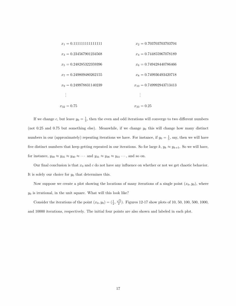
If we change c, but leave y0 = 13 , then the even and odd iterations will converge to two different numbers

(not 0.25 and 0.75 but something else). Meanwhile, if we change y0 this will change how many distinct

numbers in our (approximately) repeating iterations we have. For instance, if y0 = 15 , say, then we will have

five distinct numbers that keep getting repeated in our iterations. So for large k, yk ≈ yk+5. So we will have,

for instance, y30 ≈ y35 ≈ y40 ≈ · · · and y31 ≈ y36 ≈ y41 · · · , and so on.

Our final conclusion is that x0 and c do not have any influence on whether or not we get chaotic behavior.

It is solely our choice for y0 that determines this.

Now suppose we create a plot showing the locations of many iterations of a single point (x0, y0), where

y0 is irrational, in the unit square. What will this look like?

Consider the iterations of the point (x0, y0) = (12 ,√

22 ). Figures 12-17 show plots of 10, 50, 100, 500, 1000,

and 10000 iterations, respectively. The initial four points are also shown and labeled in each plot.

17

Figure 12: 10 iterations of (x0, y0) = ( 12,√2

2) Figure 13: 50 iterations of (x0, y0) = ( 1

2,√2

2)

Figure 14: 100 iterations of (x0, y0) = ( 12,√22) Figure 15: 500 iterations of (x0, y0) = ( 1

2,√2

2)

Figure 16: 1000 iterations of (x0, y0) = ( 12,√22)

Figure 17: 10000 iterations of (x0, y0) = ( 12,√2

2)

18

These plots emphasize the fact that the iterations of our point (x0, y0) = ( 12 ,√

22 ) really do spread out

over many areas of the unit square and do not settle down. But, we do see that there are wide gaps where

the later iterations of the points do not touch. In fact, note that our plot of 10000 iterations in Figure 17 is

strikingly similar to the plot in Figure 9 of the fourth iteration of a fine grid of points taken from the unit

square. Both are because of the way the baker map acts on a point.

The plot in Figure 17 resembles what is known as a fractal pattern. This is an important aspect of chaotic

systems. We can actually find geometrical structures associated with chaos, which tells us that chaos is not

total disorder. If it were, the iterations of the point (x0, y0) = ( 12 ,√

22 ) would fill up the whole unit square

instead of creating a pattern.

We will not go into detail about fractals, but they are important in understanding chaos, and whole

books can be devoted just to the study of fractals or the relationship between fractals and chaos.

The Double Pendulum

Now we will show how a double pendulum exhibits chaos. A double pendulum consists of two pendulums,

one hanging from a fixed point and another pendulum hanging from the first. We will consider a double

pendulum in which the masses and lengths of the two pendulums are equal. We also do not consider friction

in the system.

To talk about the position of the double pendulum, we will say that the first pendulum is at an angle θ1

from the vertical and the second pendulum is at an angle θ2 from the vertical, as shown in the drawing in

Figure 17. Note that the red circle in the drawing indicates the fixed point at which the first pendulum is

attached.

19

Figure 18: Double Pendulum

We will position two double pendulums at nearly identical locations and observe how their motion differs

over just a short period of time.

We position our first double pendulum with its first pendulum at θ1 = 3π4 radians, and its second

pendulum at θ2 = π2 radians. Our second double pendulum is placed with its first pendulum at θ1 = 3×3.14

4

radians and its second pendulum at θ2 = 3.142 radians; that is, it has been placed in nearly the same initial

position as that of the first double pendulum except that we have approximated π as 3.14. Figure 19 shows

how the motion of each double pendulum varies over a period of five seconds. Our first double pendulum is

shown in the right side of each figure, while the second double pendulum (with π ≈ 3.14) is shown on the

left side.

As can be seen in the figure, the pendulums are still in nearly the same positions after three seconds.

By four seconds, they have started to change slightly, and by five seconds they are in completely different

locations, and their locations thereafter will not be related to one another.

20

Figure 19: Motion of two double pendulums over a period of 5 seconds.

Conclusion

Chaos is everywhere in the world. This paper is meant to be a brief introduction to chaos and dynamical

systems in hopes that the reader can begin to understand what chaos is and how it can be studied. We

started by looking at the iterates of functions, stable and unstable fixed points, the graphical analysis of an

orbit, and some examples of maps and orbit diagrams. Then we discussed the Lyapunov exponent and its

importance in determining whether or not a system is chaotic. Next we went into a discussion of the baker

map, including how it acts on the unit square and at what points it exhibits chaotic behavior. Finally, we

briefly discussed an example of a more well-known but chaotic system that we can all visualize – the double

pendulum – and showed an example of how it is sensitive to initial conditions.

21

Resources

Gulick, Denny. Encounters with Chaos. New York: McGraw-Hill, 1992.

Tel, Tamas and Marton Gruiz. Chaotic Dynamics. New York: Cambridge University Press, 2006.

22

Appendix

This appendix contains the Matlab codes that were written to produce the figures in this paper.

23

24

25

The following function and code were used to produce Figures 6-9:

26

Note Figure 11 was made simply by changing the first line x0 = sym(1/2); y0 = 1/9; in the previous

code to x0 = sym(1/2); y0 = sqrt(2)/2;

27

28

29