chaos in electronic circuitsengineering.nyu.edu/mechatronics/control_lab/bck/vkapila/chaotic... ·...

Chaos in Electronic Circuits

TAKASHI MATSUMOTO, FELLOW, IEEE

lnvited Paper

This paper describes three extremdy simple electronic circuits in which chaotic phenomena have been observed. The simplicity of the circuits allows one to

i) build them easily, ii) confirm the observed phenomena by digital computer sim-

iii) rigorously prove the circuit is indeed chaotic. ulation, and in some cases

A consequence of i) is that the interested reader can build, and then see and even listen to chaos.

It is to be emphasized that these circuits are not analog computers. They are real physical systems.

I. INTRODUC~ION

Until recently, very few electrical engineers questioned the validity of the following statements:

oscillation = periodic

noise = nondeterministic

Now it is undeniable that both of them are false. The purpose of this paper is to provide the reader with not only the circumstantial evidence which has lead to questions about the validity of these statements but also a rigorous proof for it. The evidence all comes from extremely simple electronic circuits which even high school students can build. No delicate and/or expensive equipment is necessary. It is strongly recommended that the interested reader build the circuits, and then see and even listen to the phenomena. It would be a Jot of fun.

The circumstancial evidence shows that

always periodic (1.1)

and that

Manuscript received January 12,1987; revised February 5,1987. This research was supported in part by the Japanese Ministry of Education, the Murata Foundation, the Mazda Foundation, the Soneyoshi Foundation, the Institute of Applied Electricity, the Tokutei Kadai of Waseda University, and the Institute of Science and Engineering at Waseda University.

The author is with the Department of Electrical Engineering, Waseda University, Tokyo 160, Japan.

IEEE Log Number 8714776.

Hands-on experience with those circuits tells us that

there are low-order deterministic (Newtonian) systems which are ”unpredictable” (1.3)

in the sense that even an extremely small change of the initial condition eventually gives rise to an entirely different trajectory. The periodic oscillators are “predictable” in that every trajectory eventually converges to the same periodic orbit irrespective of the initial condition. Experience also shows that

those systems in (1.3) can produce “deterministic noise.”

(1.4)

So far, the word “chaos” has been intentionally avoided because there has been no unanimously accepted definition of it. If one definition were used, there would be some inconsistency, while if anothe’r were used, there would be some inconvenience, and so forth. Therefore by a ”chaotic” circuit in this paper is meant, more or less ambigu- ously, a circuit which admits a nonperiodic oscillation.

Given the extremely short period of time alloted for the preparation of this paper, it will have to be restricted to those circuits studied by the author and his colleagues, even though had it been possible, chaotic circuits studied by other people would have been included.

There will be three circuits described:

I) double scroll II) folded torus

Ill) driven R-L-Diode.

The first two are autonomous while the third one is nonautonomous. The following format will be used to describe each circuit:

A) circuitry B) experimental observations C) confirmation D) analysis E) bifurcations.

Throughout the paper, the reader’s attention is directed to the simplicity of these circuits, which allows one to

i) build them easily ii) confirm observed phenomena by computer simu-

iii) rigorously prove the circuit is indeed chaotic. lation easily and, in some cases

001a9219/~7/~1033501.00 o 1987 IEEE

PROCEEDINGS OF THE IEEE, VOL. 75, NO. 8, AUGUST 1987 1033

It should be emphasized that the circuits discussed in this paper are not analog computers. In the circuits discussed below, the voltage and current of each circuit element play critical roles in the dynamics, while in an analog computer, only the node voltages of integrators are involved in the dynamics.

II. THE DOUBLE SCROLL

The circuit to be described in this section is one of the very few physical systems which fullfil i), ii), and iii) of the last section.

A. Circuitry

The circuitry is given in Fig. l(a). It contains onlyonenon- linear element: a piecewise-linear resistor with only two breakpoints given in Fig. l(b). This circuit can be easily real-

IVR +

-

I I -

-BP VR

(b) Fig. 1. A simple autonomous circuit with a chaotic attractor. (a) The circuitry. (b) v-i characteristic of the nonlinear resistor.

ized, for example, by the circuit of Fig. 2(a), where the subcircuit Nenclosed bythe broken line realizesthepiecewise- linear resistor. Fig. 2(b) shows the measured v-i characteristic of N.

6. Experimental Observations

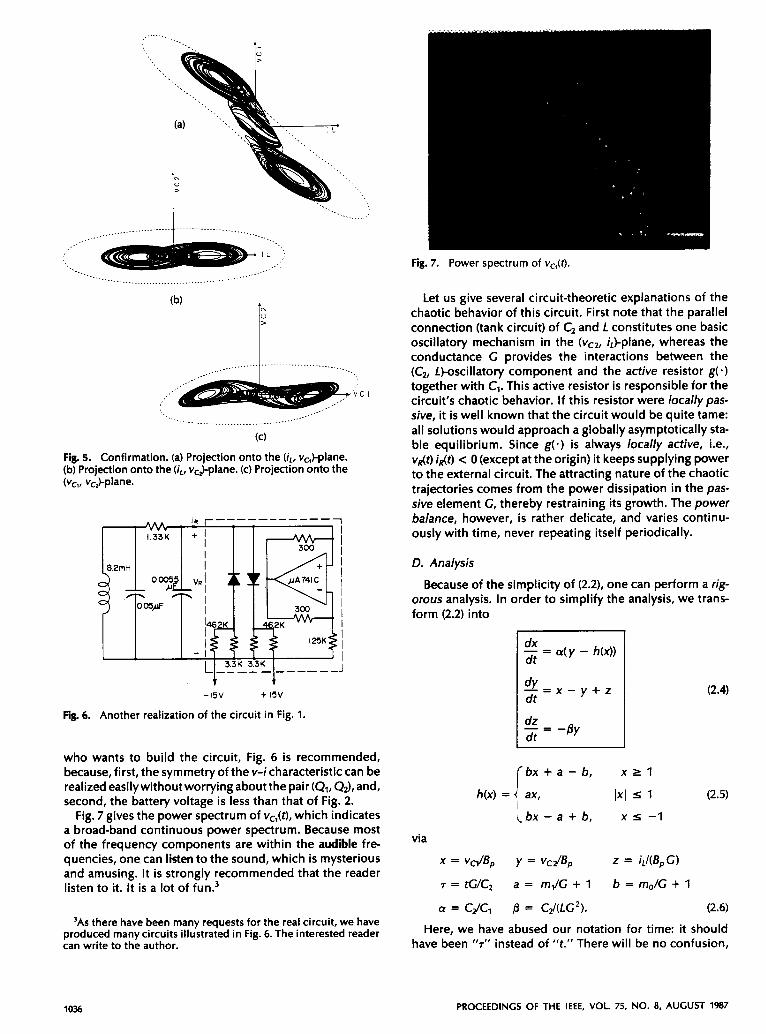
Fig. 3(a), (b), and (c) shows a trajectoryprojected onto the (iL, vcl)-plane, ( ir , vc2)-plane, and (vc,, vCJ-plane, respectively, at the following parameter values:

C, = 0.0053 pF C, = 0.047 pF L = 6.8 mH

R = 1.21 kfl RB = 56 kQ R1 = 1 kfl (2.1)

R, = 3.3 kfl R, = 88 kfl

R4 = 39 kfl Vcc = 29 V.

(b)

Fig. 2. A realization of the circuit in Fig. 1. (a) Circuitry. Q,, Q2 = 2SC1815, D,, D2 = 1S1588. (b) Measured v-i characteristic of N. Horizontal scale: 5 V/div. Vertical scale: 1 mA/ div.

Of course, they are the nominalvalues; the exact values could fall within 10 percent of these due to component tol- erances. The photographs indicate that the sotution trajectory is nonperiodic. In fact, the time waveforms of vcl(t), vc,(t), and iL(f) look like noise (Fig. +a), (b), and (c), respectively).

C. Confirmation

The dynamics of the circuit in Fig. 1 is governed by

(2.2)

where g( e ) represents the piecewise-linear characteristic of the resistor given by Fig. l(b).

The experimental observations are confirmed by solving (2.2) with the following rescaled parameter values:'

1/c, = 9 IlC, = 1 1 /L = 7 G = 0.7,

m, = -0.5 = -0.8 B, = 1. (2.3)

'Of course, one ca,n make the confirmation via the circuit of Fig. 2 by using an accurate model of the transistors, e.g., SPICE 2 [2].

1034 PROCEEDINGS OF THE IEEE, VOL. 75, NO. 8, AUGUST 1987

(C)

Fig. 3. Observed attractor. Voltage: 2 Vldiv. Current: 2 mA/div. (a) qhere is an unstable direction as well as a stable direction. Projection onto the ( iL, vc,)-plane. (b) Projection onto the ( j r , vc2)- Therefore, one cannot s e e a saddle-type periodic orbit on theoscil- plane. (c) Projection onto the (vc,, v&plane. loscope.

MATSUMOTO: CHAOS IN ELECTRONIC CIRCUITS 1035

_,.-

I L ,’

__.. ...-...-- ..._.._..._______.._.... --...-.. __...

(C)

Fig. 5. Confirmation. (a) Projection onto the (iL, v,,)-plane. (b) Projection onto the (iL, vcJ-plane. (c) Projection onto the (vel, vc2)-plane.

8.2mH

-15V t 15V

Fig. 6. Another realization of the circuit in Fig. 1.

who wants to build the circuit, Fig. 6 is recommended, because, first, the symmetryof the v-icharacteristic can be realized easilywithout worrying about the pair (Q1, Q2), and, second, the battery voltage is less than that of Fig. 2.

Fig. 7 gives the power spectrum of vc,(t), which indicates a broad-band continuous power spectrum. Because most of the frequency components are within the audible frequencies, one can listen to the sound, which is mysterious and amusing. It is strongly recommended that the reader listen to it. It is a lot of fun.3

3As there have been many requests for the real circuit, we have produced many circuits illustrated in Fig. 6. The interested reader can write to the author.

Fig. 7. Power spectrum of vcl(t).

Let us give several circuit-theoretic explanations of the chaotic behavior of this circuit. First note that the parallel connection (tank circuit) of C, and L constitutes one basic oscillatory mechanism in the (vcz, i,)-pIane, whereas the conductance G provides the interactions between the (C, Lhscillatory component and the active resistor g(-) together with C,. This active resistor is responsible for the circuit’s chaotic behavior. If this resistor were locallypas- sive, it is well known that the circuit would be quite tame: all solutions would approach a globally asymptotically stable equilibrium. Since g( . ) is always locally active, i.e., vdt) idt) e 0 (except at the origin) it keeps supplying power to the external circuit. The attracting nature of the chaotic trajectories comes from the power dissipation in the passive element C, thereby restraining its growth. The power balance, however, is rather delicate, and varies continu- ously with time, never repeating itself periodically.

D. Analysis

Because of the simplicity of (2.2), one can perform a rigorous analysis. In order to simplify the analysis, we transform (2.2) into

p x - y + z

I $ = -By

b x + a - b , x r l

1x1 s 1 (2.5)

b x - a + b , x s -1

vi a

X = v&BP y = vciBP z = iL/(BpG)

7 = tUC, a = mJC + 1 b = mo/G + 1

a = tic, 0 = C,/(LG2). (2.6)

Here, we have abused our notation for time: it should have been “7” instead of “t.” There will be no confusion,


however. Note that h ( x ) includes both x and g(x ) . We begin with the following observations:

i) Equation (2.4) is symmetric with respect to the origin, i.e., the vector field is invariant under the transformation

(x , y , z) + ( - x , - y , - a . ii) Consider the equilibria

h ( x ) = 0

{ y = O

x + z = o .

Itfollowsfromtheformofh(.)that(2.4)hasauniqueequi- librium in each of the following three subsets of R3:

Dl = { ( X , y , Z ) : X 2 I }

Do = { ( X , y , z ) : ( x J I 1)

D-1 = { ( X , y , Z ) : X I -1)

provided that a, b # -1. The equilibria are explicitly given by

P+ = ( k , 0, - k ) E Dl

0 = (0, 0, 0) E Do

P- = ( - k , 0, k ) E D-1

where k = (b - a)& + 1). iii) In each of Dl, Do, and D-l, (2.4) is linear. In fact, letting

X = (X , y , Z ) k = ( k , 0, - k )

and introducing the 3 x 3 real matrix

-ac a

Ab, 8, c) = [ i. -1 ‘1 whereA depends on a, 8, and a parameter c, which is equal toainDo,andbinD1andD-l.Wecanrecast(2.4)asfollows:

-8 0

Ab, 8, b) (X - k) , X E Dl e = { dt Ab, 8, a h , X E D O .

Ab, 8, b) (X + 4 , X E D-1

The set of parameter values (a, 8, a, b) corresponding to (2.3) is given (via 2.6)) by

(a, 8, a, b) = (9,143, -+, 3). Then the matrix

AI = A@, 14, $1 associated with the regions Dl and D-l has a real eigenvalue‘

= -3.94

and a pair of complexconjugate eigenvalues

C1 f jijl = 0.19 f j3.05.

Similarly, the matrix

A0 = A(9, 14, -;)

’The tilde is used here to distinguish the eigenvalues from the “normalized” eigenvalues which will be defined later.

associated with the region Do has a real eigenvalue

7 0 = 2.22

and a pair of complexconjugate eigenvalues

c0 f jijo = -0.97 f 12.71.

Let € ‘ ( P i ) be the eigenspace corresponding to the real eigenvalue T1 at P i and let €‘(Pi) be the eigenspace corresponding to the complex eigenvalues & f jijl at P i . Sim- ilarly, let € T O ) and €70) be the eigenspaces corresponding to To and C0 f jk0, respectively. Then the eigenspaces are given explicitly by the following equations:

€‘(Pi ) : x T k - _ - Y - Z f k --

4: + 41 + 8 41 -8

€‘(Pi): (7; + + 8) ( X T k ) + a j . 1 ~ + a(z f k ) = O

E ‘(0): X = L = f

4; + 4 0 + B 4 0 -8 EC(0): (7; + 7 0 + 8 ) x + a 4 0 y + OLZ =o.

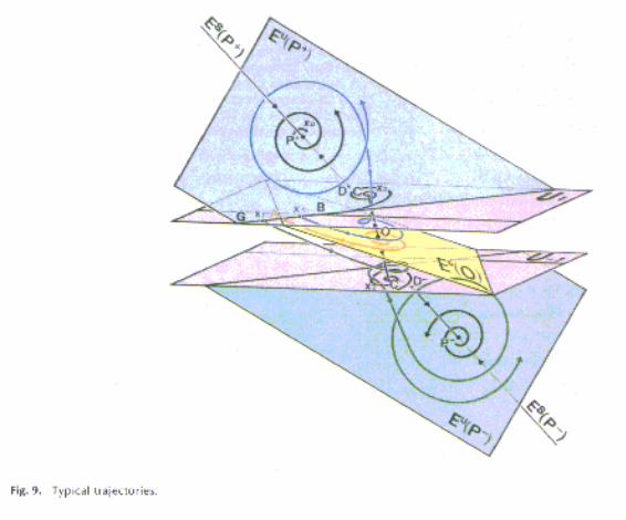
Relative positions of the eigenspaces and related sets are described in Fig. 8, where

L~ = EC(O) n u1 c = u o ) n u, L~ = E ~ ( P + ) n u1 D = E‘(P+) n u1 L~ = { X E u1 : s(x)//ul) E = L~ n L~

A = L ~ ~ L , F = {x E L 2 : f ( x ) / / L 2 } .

B = L~ n L~

Here €(x)//L2 means that the vector field ,$(x) defined by (2.4) is in parallel with Lz.

Since the dynamics is piecewiselinear, this picture (Fig. 8) already illustrates a great deal of important information as described in the following subsection.

7) Geometric Structure: Let us describe the structure of the attractor. In this subsection, we will use the following notation for the eigenspaces:

E S ( P * ) = € ‘ ( P i ) E U ( P *) = € ‘ ( P i )

ES(0) = EC(0) EU(0) = €YO).

Fig. 8. Eigenspaces of the equilibria and related sets.


Let 9' be the flow generated by (2.4) and pick an initial condition x, E E"(P+) in a neighborhood of P+. Then, for t > 0, the flow cp'(x,,) starts wandering away from Pt on EU(Pt). After winding round P+ several times in a counterclockwise direction, it hits the plane U1 at some time, say tl:xl = p"(xo). The trajectory up to tl is a spiral because (2.4) is linear in Dl and E"(Pt) is invariant. Clearly, x, E Lo. Note that the line L2 is a straight line parallel to the z-axis because x is independent of z. Observe that L2 separates the plane U, into two regions, one (to which A belongs) where x < 0 and another where x > 0. Since cp'(xo) hits the plane U1 downward (recall that the motion is counterclockwise) at t = t,, one sees that x1 belongs to the line segment m, where G is a point on Lo to the left of and sufficiently far from A, i.e., x c 0 at x,. The "fate" of cp'(xl) depends crucially on which part of x, lies (see Fig. 9).

Case 1: x, = A (red): Since the dynamics is linear in Do, one can check ana-

lytically that &) never hits U-, directly for the parameter values (2.3), i.e., the real part C0 of the complex conjugate eigenvalues is negative and small compared to the imaginary part Go. SinceA E€'(O) and since E S ( O ) is invariant, q'(xl) approaches the origin asymptotically as t + 00 (see Fig. 9). The trajectory is a spiral with an infinite number of rotations for (2.4) is linear in Do and ES(0) is invariant.

Case 2: x, E Interior (blue): In this case &x,) has two components in the sense that

its projection onto ES(0) approaches the origin asymptotically and i ts projection o n t o K c E"(0) wanders away from the origin. This means that cp'(xl) moves up along a spiral with the central axis and then eventually hits U1 again from below: x2 = @(xl). The number of rotations of &x,)

around can get arbitrarily large without bounds if xl is very close to A. These processes naturally give rise to the map

4: AB + u, defined by

*(x,) = x2.

The image *(AB) is a spiral with the center at C which is tangent to Lo at B . After hitting U,, the trajectory tp'(x2) has two components in the sense described above: one which stays in EU(P+) and moves away from P+ in a spiral manner and another in ES(Pt) which approaches P? asymptotically. Erefore,cp'(x,)ascends in aspiral path with thecentral ax is DP+ and flattens itself onto E U ( P + ) from below (see Fig. 9).

cp'(xl) has two components in the same sense as above. One component stays in €70) and asymptotically a p proaches 0 in a spiral manner. Another component stays in E U ( P t ) and moves away from 0 on c. This means that cp'(xl) descends along a spiral with the central axis c, hits U-, at x2 = cpb(xl), and eventually enters region D-,. The closer xl is to point A, the larger the number of rotations of cp'(x,) around e. After entering into D-,, the flow $(x2) consists of two components: one which is in E U ( P - ) and moves away from P-, and another which stays in E S ( P - ) and asymptotically approaches P-. Therefore, $(x2) descends spirally with the central axis D - P - and eventually flattens itself onto E Y P - ) from above (see Fig. 9).

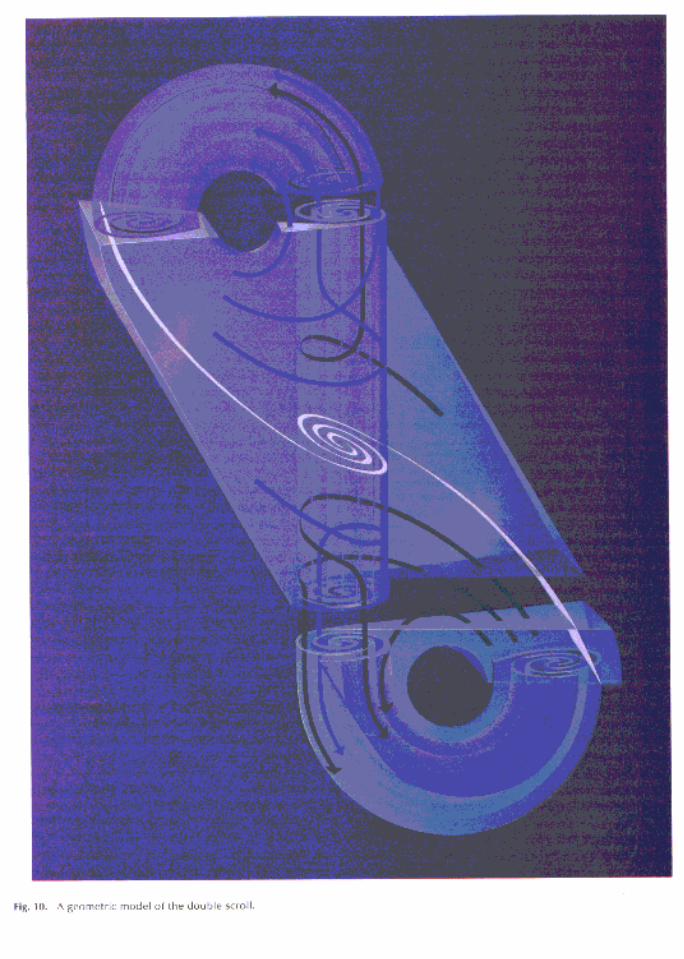
Based upon the above observations, we can understand the geometric structure of the attractor. Fig. 10 describes the structure after several simplifications. Note that two

Case 3: x1 E Interior GA (green):

-

F& 9. Typical trajectories.

1038 PROCEEDINGS OF T H E KEE,. VOL. 75, NO. 8, AUGUST 1987

Fig. 10. A geometric model of the double scroll.

MATSUMOTO CHAOS IN ELECTRONIC CIRCUITS 1039

sheet-like objects are curled up together into spiral forms: these form the "double scroll."

Let us look at a cross section of the attractor. Fig. 11 gives the cross section at vc, = 0, where the double-scroll structure is clearly seen.

Fig. 11. Cross section of the double scroll at vc, = 0.

Finally, the Lyapunov exponents [4] turn out to be

s 0.23 ~ ( 2 S= 0 p3 c -1.78

so that the Lyapunov dimension is

dL = 2 + ( p l + p2)/lp31 = 2.13.

Thisisafractalbetween2and3andagreeswiththeobserved sheet-like structure. 2) Homoclinicity: One can take full advantage of the

piecewise-linearity of (2.4) and prove that it is chaotic in the sense of Shilnikov. To begin with, recall that the line L2 denotes the set of points where the trajectory of (2.4) is tangent to U,. On the left-hand side of LZ, a trajectory hits U1 downward, while on the right-hand side of L2, a trajectory hits U, upward. Consider the trajectory starting with 0 on E'@), the unstable eigenvector. It reaches point C, which is the intersection of the unstable eigenspace of 0 with U1. If the trajectory starting from Chits a point on the line segment at some time, say (Fig. 12)

(2.7)

Fig. 12. Homoclinic trajectory at the origin.

1040

where (pf is the flow generated by (2.4), then the trajectory would stay on €YO) and asymptotically approach 0, because EC(0) is invariant. Such a trajectory is called homoclinic and it is related to a very complicated behavior of solutions to differential equations. A rigorous statement is given by the following theorem of Shilnikov ([3]-[5l):

Theorem (Shilnikov) Consider

- = fQ dx dr

where f: R3 + R3 is continuous and piecewiselinear. Let the origin be an equilibrium with a real eigenvalue y > 0 and a complex conjugate pair a f jo (a < 0, o # 0). If

i) (a1 < y, and ii) there is a homoclinic orbit through the origin

then there is a horseshoe near the homoclinic orbit. 0 The horseshoe mentioned in the theorem is formed in

the following manner. Consider Fig. 13, where an appropriate coordinate system is chosen so that the unstable eigenspace corresponds to the z-axis and the stable eigenspace corresponds to the (x , ykplane. One can take an

Fig. 13. The horseshoeembedded near the homoclinic trajectory.

appropriate cylinder and a narrow strip on the surface of the cylinder such that i ts Poincark return image is strongly contracted in the horizontal direction, strongly stretched in the vertical direction, and then bent as depicted in Fig. 13. It should be noted that a rectangle IikeA returns to the long thin object B. The horseshoe thus formed gives rise to an extremely complicated behavior. Namely, a horseshoe has a positivelyand negatively invariant setA such that [41

i) A is a Cantor set, ii) A contains a countable number of saddletype peri-

odic orbits of arbitrarily long periods, iii) Acontains an uncountable number of boundednon-

periodic orbits, and iv) A contains a dense orbit.

Moreover, a horseshoe is srructurallysrable, i.e., small per- turbations do not destroy O-iv).

Therefore, if a horseshoe is embedded somewhere in the dynamics, the trajectory will be extremely complicated. In fact, those who have experience in this area would suspect, that wherever there is chaos, a horseshoe is embedded in the vicinity of a homoclinic orbit (or a heteroclinic orbit).

3) Proof o f Chaos: One can prove rigorously [6], [q that this circuit is chaotic in the sense of Shilnikov.

PROCEEDINGS OF THE IEEE, VOL 75, NO. 8, AUGUST 1987

Theorem Consider (2.4) and (2.5) and fix

( u = 7 a = - + b = ' 7.

Then there is a j3 E [6.5, 10.51 such that the circuit is chaotic in the sense of Shilnikov.

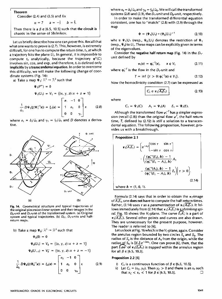
Let us briefly describe how one can prove this. Recall that what one wants to prove is (2.7). This, however, is extremely difficult, for one has to compute the return time, tl, at which a trajectory hits the plane U1. In general, it is impossible to compute tl analytically, because the trajectory cp"(C) involves sin, cos, and exp, and therefore, tl i s defined only implicitly by a transcendental equation. In order to overcome this difficulty, we will make the following change of coordinate systems (Fig. 14):

a) Take a map Pl: ?13 + Fi3 such that

*.,(P+) = 0

P1(U,) = v, = { ( x , y, z ) : x + z

rul -I O -

L

= I}

x (2.8)

where u1 = 6,/Gl and y1 = +,/G1 and D denotes a deriva- tive.

z D,-unit

(a) (b)

Fig. 14. Geometrical structure and typical trajectories of the original piecewise-linear system and their images in the &-unit and D,-unit of the transformed system. (a) Original system and typical trajectories. (b) Do-, D,-units and half- return maps.

b) Take a map Po: R3 + R3 such that

*O(O) = 0

P0(U1) = v, = { ( x , y, z ) : x + z = I}

= v,- = { ( x , y, z ) : x + z = -1)

ru0 -I O -

X

I

(2.9)

where uo = 6dGoand yo = +dGo. Wewill call the transformed systems (2.8) and (2.91, the D,-unitand Do-unit, respectively.

In order to make the transformed differential equation consistent, one has to "match" (2.8) with (2.9) through the map

aJ = ( 0 1 I Ul) O (Pol U,) - (2.10)

whc .e Q1(U, (resp., CoIU1) denotes the restriction of P1 (resp., q0) to U1. These maps can be explicitly given in terms of the eigenvalues.

Consider the negative half return map (Fig. 14) in the Dl- unit defined by

r d x ) = cpY'(X), x E Vl (2.11)

where 9;' is the flow in the &-unit and

T = inf { t > o:cp;'(x) E v1}. (2.12)

Now the homoclinicity condition (2.7) can be expressed as

F l (2.13)

where

CT = Pl(C) A1 = *1(A) €1 = PI(€). Although the transformed flow (p;'has a simpler expres-

sion (recall (2.8)) than the original flow (or, the half return time, T, defined by (2.12) is still a solution to a transcendental equation. The following proposition, however, provides us with a breakthrough.

(2.14)

where h = (1, 0, 1).

Formula (2.14) says that in order to obtain the rl-image of G, one does not have to compute the half return times. Rather, (2.14) uses T as a parametrization of rl(m). It fol- lows immediatelyfrom (2.14) that z 1 ( G ) is ashrinkingspi- ral. Fig. 15 shows the Vl-plane. The curve Q1 is a part of r l ( G ) . Several other points and curves are also drawn. They are unnecessary for the present purpose, however. The reader is referred to [6].

LetuslookatFig.l6whichistheVl-plane,again.Consider the annulus region bounded by two circles Sa and Sb. The radius of Sa is the distance of Al from the origin, while the radius of Sb is I 1 E l I I e-2ru1. One can prove [6], then, that the part of x l ( m ) is trapped within the annulus region for all j3 E [6.5, 10.51.

Proposition 2.2 [6]

i) Cl is a continuous function of B E [6.5, 10.51. ii) Let Cl = (xc, yc). Then yc > 0 and there is an xF such

that xc < xF 1 for j3 E [6.5, 10.51. 0


2.0

1.0

U.”

-1.r

-2.0

-3.u

-4.0

-9.9 -2.0 -1.0 0.0 2.)

Fig. 15. V,-plane. ~ D E ~ , ( F , B J . e , ~ l w 2 ~ l = *,(elal). -- -

e 3 , = X,(=). €4, -, - - r1(e2a2), and fl = ril(Fl). The position off, is exaggerated in this figure for clarity. The actual Posi- tion of fl is very close to a,.

Y /p‘

- 7 1 I I Fig. 16. The annulus region bounded by Sa and SL,.

Finally, if

[ and

then Proposition 2.2 ensures that

Cl (8 = 6.5) is outside of Sa

(2.15)

Cl (8 = 10.5) is inside of Sb

{C1(8 E [6.5,10.51)

is a simple curve and it intersects with x,(%) somewhere in the annulus region: homoclinicity. The final step, therefore,istoprove(2.15).Inordertodothislacomputer-assisted proof is performed.

4) Computer-Assisted Proof of (2.75): Statements in (2.15) can be written as

8 = 6.5: IIGII > IIA1II

8 = 10.5: IIClll < IIE111e-2ru1

where ul is defined in (2.8), the real part of the complex conjugate eigenvalues at P* “normalized” by the imaginary part. The projections of Al, Cl, and El onto Vl can be explicitly given in terms of the eigenvalues

A1 = (1, p1) CI = (XC, yc)

and

El = (X€, YE)

where

* { k l ~ d u l ( u ~ - 71) + 11 + 2uo71(~1 - 71))

p1 = Ul + kl(4 + lY71, kl = -7Jro

Q1 = (01 - 71)’ + 1 XE = YI(Y~ - 01 - PJQ1

YE = Y I [ ~ - (01 - rl)YQ1. The eigenvalues, in turn, are afunction of 8. The real eigenvalue Ti, i = 0, 1, is a real solution to the characteristic equation

T ; + (ac; + l)$ + (aci - a + 8 ) ~ ~ + a8ci = o where co = a, c1 = b. A simple calculation shows that the complex conjugate pair satisfy

5; = -(aci + 1 + Ti)/2

5 ; = -(aci - 1 - ~;)’/4 - a’c;/(~; + aci).

This means that given a 8, one can compute Al, C,, and El by finding zeros of polynomials of degree at most 3 and by performingtheoperations +, -, x,and +./nprinciple,this can be done by hand. However, it would be formidably tedi- ous. The computer-assistedproof given in m accuratelyesti- mates the errors incurred by

i) finding a zero of a polynomial, ii) +, -, x, t iii) conversion of a real number to and from the cor-

responding machine represented number.

The last error needs to be taken care of, since a given dec- imal number may not be machine-representable. The pro- gram in m accurately gives a lower bound and an upper bound for every value involved. In particular

8 = 6.5 llC111’ 1 2.003

> 1.557 2 lIAlI12 (2.16)

8 = 10.5: IIC1llz I 0.500

llE1ll’ 2 1.667. (2.17)

In order to take care of e-4rul, we compute the bound

-4TUl 5 -0.688

so that e-1 < e-4rUl.

1042 PROCEEDINGS OF M E IEEE, VOL. 75, NO. 8, AUGUST 1987

Because 0 e e < 3, we have

llE1112e-4*u1 > I/E1112/3 L 0.555. (2.18)

This last inequality together with (2.17) gives the desired inequality, thereby proving the homoclinicity. Inequality i) of the Shilnikov theorem can be proved by the same pro- gram together with several analyses. 0

Let us explain how the Do-unit is related to the above argu- ment. Recall Fig. 12, where we described a homoclinic trajectory. A priori, however, there is no guarantee that the trajectory, after hitting-, should not hit U - l directly, in which case the homoclinicity does not hold. In order to prove that would not happen for /3 E [6.5,10.5], we need to take care of the Do-unit where positive half return maps are needed [6]:

x;: u1 + u1 (2.19)

A;: u1 + u-1. (2.20)

Let /3* be the value of /3 at the homoclinicity. It is very important to note that even though a small change of p would destroy the homoclinicity, the horseshoe is still present, because it is structurally stable. It i s also worth noting that even though a small change in fl may destroy this particular homoclinic trajectory (Fig. 12), there are infinitelymanyval- ues of @ near /3* which give rise to other types of homoclinicity. For example, a trajectory starting with 0 on E‘(O), comes back to a point very close to 0 but not exactly, makes another round and comes back exactly to 0 (see Fig. 17).

Fig. 17. Another homoclinicity

Similarly, one can think of a homoclinic trajectory coming back to 0 after making three rounds, etc. [8]. A similar statement holds for heteroclinicity(see Section lLE7). Therefore, there is agreat number of horseshoes in (2.4) which appears to explain why chaos has been observed.

E. Bifurcations

A rich varietyof bifurcations has been observed from the circuit of Fig. 1. Fig. 18 shows the tweparameter bifurcation diagram in the (a, @)-plane, where a = -;and b = 3 are fixed. The two-parameter bifurcation diagram is generated by a rigorous bifurcation analysis described in [6] and [IOIwhere the half return maps defined by (2.10), (2.19), and (2.20) are extensively used. In order to explain what the picture means, let us fix /3 = 14 (recall that this i s the original value in (2.3)) and vary a 2 0. This essentially corresponds to fix- ing a value of the inductance L while varying the value of Cl, where CY and C1 are inversely related: a = C&. In Fig. 18, for each numbered point in the (CY, /3)-plane, the trajec-

tory projected onto the (z, x)-plane, is depicted in the box with the corresponding number.

One can show [9], [IO] that the origin is always unstable. Theotherequilibria,P*,changetheirstabilitytypedepend- ing on a. For a small value of a > 0, for example, at of Fig. 18, P* are stable and all the trajectories converge to one of them. Typical trajectories projected onto the (z, x)-plane ( ( iL , vcl)-plane) are depicted in Box in Fig. 18.

1) Hopf Bifurcation: Using the Routh formula, one can show that for

< ;(-3.5 + J(3.5)’ + 280) t 6.8.

P* and P- are stable. At

a = 3-3.5 + J(3.5Y + 280)

a pair of eigenvalues crosses the imaginary axis and Hopf bifurcation occurs, thereby signifying the birth of a periodic orbit. Hopf bifurcation here, however, should be inter- preted in its generalized sense, because the right-hand side of (2.4) is only continuous but not a C4 function. Box shows two distinct periodic attractors (stable limit cycles) at

CY = 8.0

projected onto the (z, x)-plane. Note that any asymmetric periodic attractor must occur in pair because (2.4) is syrn- metric with respect to the origin.

2) Period Doubling: As we increase CY slightly beyond 8.0, a period-doubling bifurcation is initiated. Box shows the period-2 attractors at

CY = 8.2.

A further increase of CY gives rise to period4 orbits. 3) Rossler’s Spiral-Type Attractor: At

a = 8.5

the attractor (Box ) no longer appears to be periodic. It has the structure of a Rossler’s spiral-type attractor [ I l l . As wecontinuetuningthe bifurcation parametera,weobserve that the spiral-type attractor persists up to

CY < 8.5.

4) Periodic Window: At

CY = 8.575

aperiodicwindowinBoxm isobserved.Afterthis,aspiral- type attractor is observed again.

5) Rossler’s Screw-Type Attractor: As we increase CY further, the above spiral-type attractor eventually deforms into a Rossler’s screw-type attractor [ I l l . 6) The Double Scro1l:As we increase a further, the attrac-

tor abruptly enlarges itself and creates two holes located symmetrically with respect to the origin, which corresponds to the parameter value

a = 9.0.

This i s the double-scroll attractor (see Box ). This attractor appears to persist over the parameter interval

8.81 < a < 10.05.

However, at the parameter value

a Q 10.05


Fig. 18. Two-parameter bifurcation diagram in the (a, Bkplane.


the periodic window in Box is observed. After this, several other strangelooking windows are seen. 7) Heteroclinicity: At

a J 9.78

One Observes that the “holes” Of the double scroll where vC,, vc2, and iLdenote, respectively, thevoltage across become small* In fact, the trajectory almost hits C,, the voltage across C,, and the current through L. The p* and spends an extremely long period Of time around functiong(.)denotesthev-icharacteristicofthe nonlinear P*. This signifies the heteroclinic trajectory depicted in resistor and is described by Box . One can prove the existence of a horseshoe in a manner similar to the proof given in (2.4). The heterocli- g(v) = -mov + 0.5(mo + ml) [Iv + Ell - (v - €,I]. (3.2) nicity of the double sc;oll is discussed in [6], [91, and [131.

8) Boundary Crisis: Box shows the attractor at

a = 10.5.

Suddenly, however, at

a J 10.75

the attractor disa pears: (2.4) diverges with any initial condition (see Box 6 11 )! This disappearing act provokes the interesting question as to how the attractor dies. A careful analysis suggests that this phenomenon is related to the simultaneous presence of a saddletype closed orbit encir- cling the attractor (the broken line curve in Fig. 5). With a slight increase in a beyond 10.5, the attractor appears to collide with the saddletype periodic orbit. This collision provides a natural mechanism leading to the attractor’s death. Note that if the attractor stays away from the saddletype closed orbit, there would be no way for the trajectory in the attractor to escape. If, however, the attractor collides with the saddletype closed orbit, then it would provide an exit path for the trajectory to escape into the outer space. This is what happens at a J 10.75, which signifies a boundary crisis.

Box shows the attractor at the parameter value where the homoclinicity of (2.4) occurrs. Box depicts the homoclinicity. Note that the symmetry of (2.4) implies that homoclinic trajectories are present in a pair. Finally, on the curve”Hopf at 0,” the eigenspace EC(0) changes i ts stability type, while €70) i s always unstable.

Looking at this bifurcation diagram, one sees that chaos can be quenched by making a sufficiently small, i.e., mak- ingCl sufficiently large, or makinga sufficiently large,when B is fixed. In the former case, the trajectory converges to P , while in the latter case, the trajectory converges to the large periodic attractor [I], [9]. Similarly, chaos can be quenched by adjusting fi appropriately when a is fixed.

In closing this section, there has been an interesting recent discoveryof the fact that at certain parameter values the saddletype periodic orbit is stabilized into a periodic attractor [14].

Ill. FOLDED TORUS

A. Circuitry

The circuit of Fig. 19(a) consists of only four elements among which only one is nonlinear: the piecewiselinear resistor characterized by Fig. 19(b). Linear elements L and C, are passive while the other capacitance has a negative value -Cl. The dynamics is given by

dVC, c, - = -g(v c2 - vc,) dt

Fig. 20 gives a realization. Although the capacitance on the right-hand side is positive, the subcircuit N makes it act as a negative capacitance when looked at from the left-hand port of N.

B. Experimental Observations

We will give only two pictures at two different values of Cl. Fig. 21(a) shows a 2-torus, while Fig. 21(b) indicates a

I

(b)

Fig. 19. A simple third-order autonomous circuit which exhibits a folded torus. (a) Circuitry. (b) Nonlinear resistor v-i characteristic.

-I1 Fig. 20. Physical realization of the circuit in Fig. 19.


(b)

Fig. 22. Cross sections at iL = 0, vc, < 0, of the corresponding trajectoriesfrom Fig. 20, on the(v,-,, v,-,)-plane. (a) 2-torus. (b) Folded torus.

(b) Fig. 21. Attractors observed from the circuit of Fig. 20 projected onto the (vc,, v,,)-plane. Horizontal scale: 0.5 V/div. Vertical scale: 0.5V/div. Onlyone of two attractors is shown. (a) 2-torus. (b) Folded torus.

"folded torus" [15]. In order to see them more clearly, let us look at Fig. 22 which shows the cross sections of the corresponding trajectories at iL = 0, vc2 < 0. It is clear that Fig. 21(a) is a 2-torus, while Fig. 21(b) looks like a folded torus.

C. Confirmation

Fig. 23 shows the corresponding simulation results.

D. Analysis

Let us transform (3.1) into the following dimensionless form:

_ - dx dt

- - a f ( y - x )

* = - f ( y - x ) - z dt

dz dt - = By (3.3)

where

X = v C , / E ~ y = Vc2/El z = iL/(CZEl)

a = CJC, /3 = l/(LCz) a = mo/C,

b = m,/C, (3.4)

f (x ) = -ax + 0.5(a + b) [ [ x + 11 - [ x - 111. (3.5)

The rescaled parameters which correspond to the original circuit are

a = 0.07 b = 0.1 p = 1 (3.6)

and Fig. 23(a) (resp., Fig. 23(b)) corresponds to

a = 2.0 (resp., a = 15.0).

Lyapunov exponents at a = 2.0 (resp., a = 15.0) are

ccl = 0 /LZ 0 / ~ 3 z -0.00675 (3.7)

(resp., p1 = 0.027 p2 = 0 p3 = -0.1134). (3.8)

Because no Lyapunov exponent in (3.7) is positive, the system is not chaotic. However, since only one Lyapunov expo-


Y

Fig. 23. Computer confirmation of Figs. 21 and 22. (a) Pro- jection onto the (v,,, vcz)-plane at a = 2.0. (b) Projection onto the (v,,, v,,)-plane at a = 15.0. (c) Cross section at i, = 0, vcz e 0, where a = 2.0. (d) Cross section at iL = 0, vcz 0, where a = 15.0.

nent is negative, the solution is not a periodic attractor, either. The presence of 2 zero Lyapunov exponents, therefore, prqiiides a further confirmation that the trajectory in

is indeed a 2-torus, namely, a quasi-periodic solution. Fig* 2Y he largest Lyapunov exponent pl in (3.8) is positive, whi ih confirms that the trajectory in Fig. 21(b) is chaotic.

Let us look at typical trajectories in terms of the eigenspaces of equilibria as we did for the double scroll. First we partition the state space into three regions R1, Ro, and R-1

separated by boundaries 61 and 6-1, respectively, where (see Fig. 24)

R' = {(x, y, z):y - x < - I }

Ro = {(x, y,z):(y - XI < 1)

R-1 = {(x, y, z):y - x > I }

B' = {(x, y, z):y - x = - I }

6-1 = {(X, y, Z):Y - X = 1).

System (3.3) has three equilibria, 0 and f * . The eigenvalues atO(resp.,ff)consistofonerealj.o(resp.,rl)andacomplex- conjugate pair Co f /Go (resp., C1 f jG1). In particular at a = 2,@ = 1

T o J 0.14786 60 = -0.048886 Go J 1.o060

j.' = -0.10425 51 J 0.034426 131 = 1.0030. (3.9)

Let ES(0) (resp., E"(0)) denote the eigenspace corresponding to To (resp., c0 f io,,). Similarly, let E " ( f * ) (resp., E'(P*) ) denote the eigenspace corresponding to C1 * j G l (resp., T1). While the patterns of the eigenvalues in (3.9) are identical to those of the double scroll, there are two subtle dif- ferences:

i) The magnitude of lqll is not as large as in the double

Fig. 24. Typical trajectories.

scroll, hence the "flattening" of the attractor onto EU(P i, is relatively weak.

ii) P(O) and €"(Pi) are almost parallel with each other.

Let ( p f be the flow generated by (3.3) and pick an initial condition x. near 0 above €70) but not on €YO). Since To > 0, cp'(xd starts moving up (with respect to the x-axis) while rotating clockwise around €'YO) (Fig. 24). Since (3.3) is linear in R,,, cp'(xo) eventually hits 61 and enters R1. Because of the relative position of ES(P *), (p'(x0, further moves up while this time rotating around E S ( P + ) . Since tl > 0, the solution cp'(x0) increases i ts magnitude of oscillation and eventually enters R,,. Then, because of the relative positions of &and R1, cp'(xo) starts moving downward.(with rotation), eventually hits 6-1, and then flattens itself against ES(0) while rotating around E"(0). Since Co < 0, the solution decreases its magnitude of oscillation and gets into the original neighborhood of 0. This process then repeats itself, ad infinitum, but never returning to the original point. Hence the associated loci densely cover the surface of a two-torus.

€. Bifurcations

Bifurcations of (3.3) are extremely rich. They even include the double scroll. Note that (3.3) and (3.5) have four parameters. We will fix a and b as in (3.6) and vary a and 0. The appearance of a 2-torus indicates that one can look at the bifurcations in terms of rotationnumben. The rotation num- berp is defined for a homeomorphism b on a circle, namely

h: S' + S'

p = lim h"(X) - X , x E s'.

n+oo n

(The limit always exists.) If p is rational, i.e., p = mh, where m and n are positive integers, then the trajectory is n-periodic. In this case, all trajectories approach a unique n-periodic orbit, while winding around S' "m"times before com- pleting one periodic orbit. Such behavior is called an m: n phaselocking. If p is irrational, then the orbit is quasiperiodic and, therefore, densely covers S'.

In order to study the rotation number for (3.3), one has to find a subset homeomorphic to S' and that a homeomorphism h is indeed induced via the flow of (3.3) on it. Since this is an extremely difficult, if not impossible task, we assume that the rotation number can be defined in the following region:

{(a, B ) I I < a < b(a))


where b(a) is a function which describes the curve €3 of Fig. 25, the bifurcation diagram. Let us explain Fig. 25 in more detail. On the line DIVwhich is the line a = 1, the divergence of (3.3) is zero. For 0 < a < 1, a periodic attractor is observed, while for a > 1, an attracting torus is observed (Fig. 22(a)).

The solid lines indicate the boundaries of the regions where the rotation numbers are constant, where 1 : 5 means that the rotation number p = i , etc. The chain lines denote curves on which perioddoubling bifurcations occur. In order to avoid further complication of the picture, only the onset of the perioddoublingcascade is shown. The broken lines indicate boundaries where chaos is observed. The symbol Cstands for (folded torus) chaos whereas DS stands for the double scroll. These curves are obtained by observing the trajectories via Runge-Kutta iterations. Note that thereare many regions in Fig. 25wherethe rotation number is equal to some rational number. Such regions are called Arnold tongues.

A careful examination of Fig. 25 reveals the following empirical laws (for fixed 8):

i) If a1 > a2 and if p(al) = mJnl, p(az) = mJn2, then

ii) There is an a3 such that a1 > a3 > a2, p(a3) = p(a1) < p(a2).

(ml + m2)l(nl + nd, and

p(a1) > dad > p(a2).

Fig. 26 gives the graph of p as a function a with 8 = 1. The resulting monotone-increasing function is called a devil’s staircase. The graph is obtained by observing the trajectories via Runge-Kutta iterations.

In order to get a feeling of what is happening, let us fix 8:

B = 1

and vary a:

0 < a < 14.3.

Fig. 27 shows the bifurcation diagram of vc, on the cross section iL = 0, vc2 c 0. Let us explain this in terms of Fig. 25.

i) As one moves along 8 = 1 in the 1 :5 Arnold tongue, one hits the boundary of the 2: 10 Arnold tongue, thereby signifying a perioddoubling bifurcation.

ii) When one moves to the right in the 1 :6Arnold tongue onthelineB=l,onedoesnothittheboundaryofthe2:12 Arnold tongue. This explains why one does not observe any period-doubling cascade for the period-6 attractor.

iii) As one moves to the right along the line = 1, the circle map nature is destroyed before the system gets into the 1 :6 phase-locking. This is why one observes a sudden bifurcation of 1 :6 phase-locking into chaos. It appears that this chaotic attractor is born via an intermittency route. After 1 :6 phase-locking, i.e., after all fixed points disappear via a tangent bifurcation, there are six regions called “chan- nels.” Inside each channel, a solution behaves like a periodic orbit because it spends a very long period of time in the channel. Once it gets out of the channel, however, the solution behaves in an erratic manner. Finally, we remark that the 1 :5 Arnold tongue overlaps with the 1 :4 Arnold tongue, hence the right-hand boundary of the 1 :5 Arnold tongue cannot be observed clearly.

It should be noted that the above bifurcation scenario indicates a “torus breakdown” in the third-order autonomous circuit. Previous systems in which torus breakdowns have been observed are either nonautonomous [16], 1171 or higher order [ M I , [19]. Also, previous work on torus breakdowns has been, to the best of our knowledge, either through laboratory measurementonly[l6] or by simulation

0 1 x) 20 30 m a

Fig. 25. Two-parameter bifurcation diagram in the (a, @)-plane.

PROCEEDINGS OF THE IEEE, VOL. 75, NO. 8, AUGUST 1987

6pO 1

S El

9 st

L Ll 61 U

8 6 01 11

D 001 0'5 0'0

d

R L

P Fig. 28. Driven R-L-Diode circuit. R = 107 Q, L = 2.5 mH, f = 150 kHz, Diode: 3CC13.

B. Experimental Observations

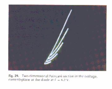
Fig.29showsthetwo-dimensionalPoincar6sectiontaken at each period T = l / f i n the (voltage, current)-plane of the diode.

Fig. 29. Two-dimensional Poincare section in the (voltage, current)-plane of the diode at E = 6.2 V.

C. Confirmation

Although the circuit in Fig. 28 contains only three elements, its dynamics is rather involved in view of the non- linearities of the p n junction diode, which are not purely resistive at frequencies above 100 kHz. A reasonably accurate circuit model of the diode [21] is given by Fig. 30, where both the resistor and the capacitor (Fig. 30(b)) are nonlinear. From extensive laboratory measurements and digital computer simulations, it has been observed [22] that in order to reproduce the same qualitative behavior, the nonlinear resistor in the above model is not essential. Moreover, the nonlinear q-vcharacteristic of the capacitor can be replaced by the drastically simpler two-segment piecewise-linear curve shown in Fig. 30(c), without changing the bifurcation pictures.

Fig. 31 showsthe simulation correspondingto Fig. 29.The cross section, however, is taken on the (charge, current)- plane instead of the (voltage, current)-plane, due to a lack of time to prepare the material.

D. Analysis

Toanalyzethecircuit,wewillfurthersimplifythedynam- ics, and then observe several key properties of the Poincark

p ' O r -

L ' I b I

7F i2 (b) (C)

Fig. 30. Circuit model of a diode. (a) Original model (parallel connection of a nonlinear resistor and a nonlinear capacitor). (b) Characteristic of the nonlinear capacitor. (c) A drastically simplified capacitor characteristic without destruction of the essential features.

return map. Based upon these observations, we will propose a surprisingly simple two-dimensional map model which essentially captures the bifurcation pictures of the original circuit.

1) Further Simplification: In order to understand how a chaotic attractor is formed, we will further simplify the circuit of Fig. 28 with Fig. 30(c). Namely, we have observed that the sinusoidal voltage source can be replaced by a square- wave voltage source of the source period T = I / f without altering the essential features. Therefore, we will analyze the circuit shown in Fig. 32 where the nonlinear capacitor is characterized by Fig. 30(c). The dynamics of this circuit is described by

- = I dQ dr

i f Q r O

i f Q < O

i f n T s r < ( n + : ) T )

where we use Q, I, and r to denote the original circuit variables. Defining the following normalized variables:

R 1 1 L f

k = - a=- LC,f2

p = - LC2f2' (4.2)


-1 .00 0.60 2 . 2 0 3.80 5 . 4 0 7.00 8.60 10.20 GI( NC 1

Fig. 31. Confirmation. The cross section is taken on the (charge, current)-plane instead of the (voltage, current)-plane.

R L

1. Fig. 32. Simplified circuitwhich capturesessentiallyall the experimentally observed phenomena.

Equation (4.1) can be transformed into

9:: q 2 0 and the driving source is V,(t) = -1

9:: q < 0 and the driving source is V,(t) = -1.

Using the above simplified circuit model and solution components, we can uncover the essential features of the circuit dynamics with the help of the following observations:

i) The area contraction rate is constant and is strictly less than 1. This stems from the fact that the area contraction rate is determined by the divergence of (4.3), namely

area contraction rate = exp (divergence) where divegence = - k = - R / L f . (4.4)

ii) 0 5 t < 1/2. Fig. 33 shows the flows cp: and cp: with a = 0.1, /3 = 10.0.

Each trajectory corresponds to a different initial condition.

First observe that any solution of (4.3) is made up of components from the following four linear autonomous flow son

I I, \ ', L,,

2 2 4 \ * \ \ , ' ~ \

pi: q 2 0 and the driving source is Vs(t) = +I

9:: q < 0 and the driving source is Vs(t) = +I Fig. 33. Deformation of the initial rectangle A along a trajectory for 0 5 t 5 ID.


Consider the trajectory E, which passes through the origin. Picka"thin"rectangleAatt=Oasshowninthefigureand look at how A is deformed along the flow cp: as t increases. If the initial condition (qo, io) E A lies to the right-hand side of E, then &90, io) never hits the i-axis. On the other hand, if (qo, io) lies on the left-hand side of E, then ~$(90 , io) eventually hits the i-axis at some time t, > 0; namely, (q,, il) = q$(q0, io). For t > tl the dynamics obeys the flow cp: where eventually it again hits the i-axis at some time tz > t,; namely, (92, iz).= g(91, i,), whereupon it reverts back to the original flow 0: for t > tz. The key observation here is that a < fl implies that the vertical velocity (i.e., the i-axis) component of trajectories corresponding to cp: is larger than that for 9:. This implies that the part of A which is on the left-hand side of E is stretched (in the vertical direction) more than the part on the right-hand side of E. Note also that on the left- hand side of E, 4; < 91 implies that &(q;, il) has a larger vertical stretching than &ql, i,). These observations show that A is eventually deformed into sets B and C shown in Fig. 33.

iii) 1/2 I t < 1. After t = 112, the dynamics consists of component flows

given by Fig. 34. Extensive computer simulations show that

Fig. 34. Deformation of the set C along a trajectory for 1/2 s t 5 1.

for 112 I t < 1, the set &C) never hits the i-axis if the initial rectangle A in Fig. 33 is chosen appropriately.

Combining the above three observations, we see that during the period 0 I t < 1, rectangle A stretches, folds, and eventually returns to the original region D. Extensive numerical observations show that we can choose appro- priateA and D such that A 3 D. During this transformation process,theareaofAiscontinuallybeingcontracted.Ifthis mechanism is repeated many times, it can give rise to a very complicated behavior, such as chaos. Fig. 35 gives a global picture of this transformation over one period of the flow

2) TweDimensional Map Model: Based upon the preceding observations, we propose a surprisingly simple two- dimensional map model which mimics the transformation described in Fig. 35. Fig. 36 gives a more precise description of the transformation mechanism. A simple two-dimensional map which transforms the square STUV in Fig. 36(a) into the lambda shaped set in Fig. 36(d) is described by

Ot.

a,x,, if x, 2 0) x,+, = Yn - 1 +

-+x,,, if x, < 0

+ 1 i

I I

Fig. 35. Overall picture of how the initial rectangle A i s deformed and eventually returns to the initial region.

(a) (b) (C) (dl Fig. 36. Two-dimensional map model. (a) The initial rectangle STUV. (b) The initial rectangle is compressed in the vertical direction. (c) The compressed rectangle is rotated by 90°. (d) The rectangle is bent into a lambda shape.

This map captures all the essential features of the bifurcations observed from the original circuit as shown in the following subsection.

E. Bifurcations

Fig. 37 gives an experimental observation showing the ondimensional bifurcation diagram of thecurrent iof the circuit of Fig. 28 when the amplitude E of the applied sinusoidal voltage source is increased periodically from 0 to7.7VIEismodulated byasawtoothwaveform).Eachpoint in this "bifurcation tree" represents a one-dimensional Poincark section taken at each fundamental period T = l l f o f the sinusoidal source. There are two striking features in this bifurcation tree:

i) A succession of large periodic windows the periods of which increase exactybyone as we move from any window to the next window to the right.

ii) A succession of chaotic bands sandwiched between the large periodic windows.

The cross section in Fig. 29 corresponds to E = 6.2 V, i.e., thefivechaoticbandsofFig.37correspondtothefive"legs" of Fig. 29.

Let us examine how the simple map (4.5) captures the essential features of the bifurcation phenomena observed experimentally from the R-L-Diode circuit. Fig. 38 shows the one-parameter bifurcation diagram of x for (4.5) where

a, = 0.7 b = -0.13

and a2 is varied over the range

0 5 a2 5 20.

1052 PROCEEDINGS OF THE IEEE, VOL 75, NO. 8, AUGUST 1987

Fig. 37. One-dimensional bifurcation diagram of current i when amlitude E is increased from 0 to 7.7 V.

X

a2

Fig. 38. One-parameter bifurcation diagram ofxforthetwo- dimensional map model where 0 5 a, I 20.

Fig. 39 shows the attractor in the ( x , y)-plane corresponding to

a2 = 18.0.

Note that the attractor is qualitatively identical to the one obtained experimentally in Fig. 29.

A detailed analysis of (4.5) can be performed because of its simplicity. Based upon the bifurcation analysis of (4.5) one can understand the bifurcations of the original circuit. Fig. 40 shows the detailed bifurcation mechanism associ- atedwith theperiod4window. Bifurcationsassociated with other periodic windows have similar structures. The sequence of drawings in column B of Fig. 40 shows how the attractor of the two-dimensional map model is deformed as a2 is increased from its value at the lowest position to a

X

Fig. 39. Attractor observed from the two-dimensional map model at a, = 18.0.

larger value at the top position. The’knapshots” in column A show the corresponding experimental observations taken from the original R-L-Diode circuit as E increases from the bottom. The four insets in column Care enlarged pictures in a small neighborhood of the periodic point P4A (of the two-dimensional map) identified by the solid triangles A.

Wecan nowgiveacomplete pictureofwhat is happening in the original circuit.

i) Let us begin with the picture at the bottom in column Band look at the folded object. The symbol * identifies the location of the fixed-point Qof (4.5) which is a saddle point for the present parameter range. As we increase the value of a2 ( E in the original circuit), a saddlenode bifurcation of period4 takes place outside the region where the attractor lives. This period4 orbit has a strong influence on the

MATSUMOTO CHAOS IN ELECTRONIC CIRCUITS 1053

A B Fig. 40. Detailed bifurcation mechanisms corresponding to the period4 window. Col- umn Agives experimentally measured pictures, while the insets in column C show blown up pictures around P4A.

C

1054 PROCEEDINGS OF T H E IEEE, VOL. 75, NO. 8, AUGUST 1987

“structure” of the attractor. Since the bifurcation in this case corresponds to that of a saddle-node, a stable and unstable periodic orbits are born in pairs of one each.

ii) As we increase a2 further, the unstable periodic orbit moves closer and closer to the attractor, and finally it collides with the attractor. This is depicted in the next to the last picture in column B, where the solid triangles A (resp., open dots 0) correspond to an unstable (resp., stable) periodic orbit. The three insets in column C show the situation around the right-most unstable periodic point denoted by P4A.5 The bottom inset (in column C ) shows the situation before collision, where thick lines indicate W& the unstable manifold of Q(the closure of which is conjectured to be the attractorL6 As one increases a2 by an appropriate amount, one sees that

W t collides with w:4A (4.6)

where WSp4* denotes the stable manifold of P4A. This is shown in the second inset from the bottom in column C, where W& is denoted by thick lines. A slight increase of a2 leads to the situation depicted by the third inset from the bottom in column C, where, this time, Wlj is indicated by thick broken lines. The crucial observation in this picture is that the unstable direction of P4A provides an orbit with an exit gate to escape into the outer region. Because the stable and the unstable manifolds are invariant, a collision of the attractor with P4A is equivalent to a collision of the attractor with wsP4A.

iii) As there is now an exit gate, the attractor can no longer survive. Consequently, we observe the sudden disappear- ance or extinction of the attractor at the critical parameter value given by (4.6). This phenomenon, therefore, represents acrisis. After escaping into the outer region, however, the orbit cannot diverge to infinity because the stable periodic orbit is waiting to attract it. This situation is depicted in the third picture from the bottom in column B. This is the mechanism responsible fortheextinction (death)of the “two-legged” attractor and the simultaneous emergence (birth) of a stable period4 orbit.

iv) As we increase a2 further, the stable period4 orbit loses its stability via aperiod-doubling bifurcation. The lim- iting periodic attractor then changes into a chaoticattractor madeupoffourisletsasdepicted inthefourth picturefrom the bottom in column B. The destablized periodic points are denoted by four solid dots 0 . Observe that the chaotic attractor in this case is the closure of the unstable manifold of 0 ratherthanthatof * (seei)). Notealsothattheunstable period4 points represented by the 4 solid triangles A born in the preceding picture are still present near the chaotic attractor.

v) As we increase a2 even further, the chaotic attractor eventually collides with the stable manifold of A; namely,

’Since this is a saddle-node bifurcation, a stable period4 orbit and an unstable period4orbit are born simultaneously. Oneof the stable periodic points is denoted by P4B, whereas one of the unstable periodic points is called P4A.

%enerally it is conjectured [4] that a chaotic attractor is the closure of the unstable manifold of a periodic point. In fact, Misiu- rewicz [23] proved this fact rigorously for a piecewise-linear two- dimensional map (the Lozi map) which is similar to (4.5). Extensive simulations suggest that this appears to be the case for (4.5) as well.

WF4, collides with WSp4A. (4.7)

This is depicted in the third picture from the bottom in column B. The corresponding inset in column C shows the blown-up details around P4A. When (4.7) occurs, WF4B plays the role of “bridging” between the chaotic islands, thereby giving birth to the attractor with “three legs“ shown in the topmost picture in column B. Note that the increase in the number of legs (or the number of islands in the chaotic bands) is attributed to the interaction of the attractor with the other perioddorbit which was born earliervia a saddle- node bifurcation.

Details of this section are found in [24], [25].

V. REMARKS

There is another interesting circuit [26] which cannot be included in this article due to the space limitation. The circuit exhibits a hyperchaos [27l, i.e., it exhibits a chaotic attractor with more than one positive Lyapunov exponents. In other words, the dynamics expands not only small line segments but also small area elements, thereby giving rise to a “thick” attractor. This circuit appears to be the first real physical system where a hyperchaos has been observed experimentally and confirmed by computer. The reader is referred to [26].

The circuits described in this article are so simple that there must have been electrical engineers who”saw”chaos on their oscilloscopes and yet did not “recognize” it for what it was.7 One cannot recognize a fact without having the corresponding concept.

The reader who has read this paper as well as other papers in this special issue, would understand (1.3)and (1.4)aswell as (1.1) and (1.2), while in the past, only very few people (Poincare, Birkoff, Einstein, and several others) were aware of them.

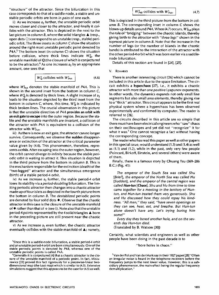
Finally, there is a famous story by Chuang Tsu (369-286 B.C.) (Fig. 41):

The emperor of the South Sea was called Shu [Briefl, the emperor of the North Sea was called Hu [Sudden], and the emperor of the central region was called Hun-tun [Chaos]. Shu and Hu from time to time came together for a meeting in the territory of Hun- tun, and Hun-tun treated them very generously. Shu and Hu discussed how they could repay his kind- ness. ”All men,” they said, “have seven openings so they can see, hear, eat, and breathe. But Hun-tun alone doesn’t have any. Let‘s trying boring him some!”

Every day they bored another hole, and on the sev- enth day Hun-tun died. (Translated by B. Watson [30])

Certainly, what scientists and engineers as well as other people have been doing in the past decade is to

“bore holes in chaos.”

’Van der Pol and Van der Mark say in their 1927 paper [28]“0ften an irregular noise is heard in the telephone receivers before the frequency jumps to the next lower value. However, this is a sub- sidiary phenomenon, the main effect being the regular frequency demultiplication.”


‘f

. !2 I ’

Fig. 41. Chuang Tsu’s story of chaos [29].

10%

This, however, is the very thing they have been doing to everything mysterious all the time. When the mystery is eventually cleared up by analysis, characterization, proof, etc., it ceases to be a mystery; it is objectified. The word “death“ should perhaps be understood in this sense.

ACKNOWLEDGMENT

Theauthorwould l iketothankal l h is f r iendswho k ind led his fascination in chaotic circuits. Among them are L. 0. Chua of U. C. Berkeley, M. Komuro of Numazu College of Technology, Y. Togawa of Science University of Tokyo, H. Kokubu and H. Oka of Kyoto University, M. Hasler of Swiss Federal Institute of Technology, Y. Takahashi of Tokyo Uni- versity, I. Shimada of Nihon University, C. lkegami of Nagoya University, M. Ochiai of Shohoku Institute of Tech- nology, K. Sawada of Toyohashi University of Technology and Science, S. Tanaka and T. Suzuki of Hitachi, S. lchiraku of Yokohama City University, K. Kobayashi of Matsushita, as well as R. Tokunaga, K. Ayaki, K. Tokumasu, T. Makise, T. Kuroda, and M. Shimizu of Waseda University.

REFERENCES [I] T. Matsumoto, L. 0. Chua, and M. Komuro, “The double

scroll,” /E€€ Trans. Circuits Syst., vol. CAS-32, pp. 797-818, Aug. 1985.

[2] T. Matsumoto, L. 0. Chua, and K. Tokumasu, “Double scroll via a two-transistor circuit,” / F E E Trans. Circuits Syst., vol. CAS- 33, pp. 828-835, Aug. 1986.

[3] L. P. Shilnikov, “A case of the existence of a denumerable set of periodic motions,” Dokl. Sov. Math., vol. 6, pp. 163-166, 1965.

[4] J. Cuckenheimer and P. Holmes, Nonlinear Oscillations, Dynamical Systems, and Bifurcations of Vector Fields. New York, NY: Springer-Verlag, 1983.

[5] A. Arneodo, P. Coulett, and C. Tresser, “Oscillators with chaotic behavior: An illustration of a theorem by Shilnikov,” 1. Stat. Phys., vol. 27, pp. 171-182,1982.

[6] L. 0. Chua, M. Komuro, and T. Matsumoto,”The double scroll family,” IEEE Trans. Circuits Syst., vol. CAS-33, no. 11, pp. 1073- 1118, Nov. 1986.

m T. Matsumoto, L. 0. Chua, and K. Ayaki, in preparation. [8] P. Glendinning and C. Sparrow, “Local and global behavior

near homoclinic orbits,” 1. Stat. Phys., vol. 35, pp. 645-697, 1984.

[9] T. Matsumoto, L. 0. Chua, and M. Komuro, ’The double scroll bifurcations,” lnt]. Circuit TheoryAppl., vol. 14, pp. 117-146, Apr. 1986.

[IO] -, “Birth and death of the double scroll,” Physica D, in

[ l l ] 0. E. Rossler, “Continuous chaos-Four prototype equa- press.

tions,” Ann. N.Y. Acad. Sci., vol. 316, pp. 376-392, 1979. [I21 C. Crebogi, E. Ott, and J. Yorke, “Chaotic attractor in crisis,”

Phys. Rev. Lett., vol. 48, pp. 1507-1510,1982. [I31 A. I . Mees and P. B. Chapman, “Homoclinic and heteroclinic

orbits in the double scroll attractor,” to be published in / F E E Trans. Circuits Syst., vol. CAS-34, no. 9, Sept. 1987.

[I41 D. P. George, “Bifurcations in a piecewise linear system,” Phys. Lett. A, vol. 118, no. 1, pp. 17-21,1986.

[15] W. F. Langford, Numerical Studies of Torus Bifurcations (International Seriesof Numerical Mathematics, vol. 70) Hei- delberglNew York: Springer-Verlag, pp. 285-295.

[I61 J. Stavans, F. Heslot, and A. Libchaber, “Fixed winding number and the quasi-periodic route to chaos in a convective fluid,” Phys. Rev. Lett., vol. 55, no. 6, pp. 596-599, Aug. 5,1985.

[ I 7 T. Bohr, P. Bak, and M. Hogh Jensen, “Transition to chaos by interaction of resonances in dissipative system II. Josephson junctions, chargdensity waves, and standard maps,” Phys. Rev. A, vol. 30, no. 4, pp. 1960-1969, Oct. 1984.

[I81 M. Sano and Y. Sawada, ‘Transition from quasi-periodicity to chaos in a system of coupled nonlinear oscillator,” Phys. Lett., vol. 97A, no. 3, pp. 73-76, Aug. 15, 1983.

PROCEEDINGS OF THE IEEE, VOL. 75, NO. 8, AUGUST 1987

[19] V. Franceschini, “Bifurcation of tori and phase locking in a dissipative system of differential equations,” Pbysica 6D, pp.

[20] T. Matsumoto, L. 0. Chua, and R. Tokunaga,”Chaosviatorus breakdown,” I€€€ Trans. Circuits Syst., vol. CAS-34, pp. 240- 253, Mar. 1987.

[21] €/electronics Designer’s Handbook, 2nd ed. New York, NY: McCraw-Hill, 1977.

[22] T. Matsumoto, L. 0. Chua, and S. Tanaka, “Simplest chaotic nonautonomous circuit,” Pbys. Rev. A, vol. 30, pp. 1155-1158, 1984.

[23] M. Misiurewicz, “The Lozi mapping has a strange attractor,” Ann. N.Y. Acad. Sci., vol. 316, pp. 348-358, 1979.

[24] T. Matsumoto, L. 0. Chua and S. Tanaka, “Bifurcations in a driven R-L Diode circuit,” in Proc. / € € E Int. Syrnp. on Circuits and Systems, pp. 851-854, 1985.

[25] 5. Tanaka, T. Matsumoto, and L. 0. Chua, “Bifurcation scenario in a driven R-L Diode circuit,” Pbysica D, in press.

285-304,1983.

[26] T. Matsumoto, L. 0. Chua, and K. Kobayashi, “Hyperchaos: Laboratory experiment and numerical confirmation,” / E € € Trans. Circuits Syst., vol. CAS-33, no. 11, pp. 1143-1147,1986.

[27] 0. E. Rossler, “Chaotic oscillations-An example of hyperchaos,” in Nonlinear Oscillations in Biology (Lectures in Applied Mathematics, vol. 17). New York, NY: Amer. Math.

[28] E. Van der Pol and I . Van der Mark, “Frequency demultiplication,” Nature, vol. 120, no. 3019, pp. 363-364, 1927.

(291 1525 Chinese Edition (printed during the Ch’ing Dynasty). [30] B. Watson, The Cornp/ete Works of Cbuang Tsu. New York,

SOC., 1979, pp. 141-156.

London: Columbia Univ. Press, 1968.

Takashi Matsumoto (Fellow, IEEE), for a photograph and biography, please see page 981 of this issue.


chaos in electronic circuitsengineering.nyu.edu/mechatronics/control_lab/bck/vkapila/chaotic... ·...

Documents