Chaos theory and time series analysis

Molenaar, J.

Published: 01/01/1992

Document VersionPublisher’s PDF, also known as Version of Record (includes final page, issue and volume numbers)

Please check the document version of this publication:

• A submitted manuscript is the author's version of the article upon submission and before peer-review. There can be important differencesbetween the submitted version and the official published version of record. People interested in the research are advised to contact theauthor for the final version of the publication, or visit the DOI to the publisher's website.• The final author version and the galley proof are versions of the publication after peer review.• The final published version features the final layout of the paper including the volume, issue and page numbers.

Link to publication

Citation for published version (APA):Molenaar, J. (1992). Chaos theory and time series analysis. (IWDE report; Vol. 9205). Eindhoven: TechnischeUniversiteit Eindhoven.

General rightsCopyright and moral rights for the publications made accessible in the public portal are retained by the authors and/or other copyright ownersand it is a condition of accessing publications that users recognise and abide by the legal requirements associated with these rights.

• Users may download and print one copy of any publication from the public portal for the purpose of private study or research. • You may not further distribute the material or use it for any profit-making activity or commercial gain • You may freely distribute the URL identifying the publication in the public portal ?

Take down policyIf you believe that this document breaches copyright please contact us providing details, and we will remove access to the work immediatelyand investigate your claim.

Download date: 28. May. 2018

Report IWDE 92-05

Chaos Theory and Time Series Analysis

J. Molenaar

May 1992

INSTITUUT WISKUNDIGE DIENSTVERLENING EINDHOVEN

Report IWDE 92-05

CHAOS THEORY

AND

TIME SERIES ANALYSIS

J. Molenaar

Lecture Notes, May 1992

Eindhoven University of Technology Faculty of Mathematics and Computing Science P.O. Box 513 5600MB Eindhoven The Netherlands Tel : +31 40 474757/474760 Telefax : +31 40 442150 E-mail : jaapm@win.tue.nl

ii

Contents··

1. INTRODUCTION 1

la. The Oimate

lb. The Dripping Faucet

lc. The Logistic Equation

2. DYNAMICAL SYSTEMS FOR T ~ oo 9

2a. Conservative Systems

2b. Dissipative Systems

2b.l Point Attractors

2b.2 Periodic Attractors

2b.3 Quasi-Periodic Attractors

2b.4 Chaotic Attractors

2b.5 Structure of Chaotic Attractors

3. FRACTAL DIMENSION 16

3a. Numerical Estimation of doap

3b. Numerical Estimation of d.,.

3c. Noise

3d. Dimension Estimation and Principal Component Analysis

4. LYAPUNOV EXPONENTS 20

4a. ~ for One-dimensional Systems

4b. ~ for n-dimensional Systems

4c. Numerical Calculation of ~

4c.l Calculation of A.1 from Model Calculations

4c.2 Calculation of ~ from Data

5. THE RECONSTRUCTION PROBLEM 25

5a. Estimation of the Embedding Dimension

Sb. Estimation of Delay k.

5c. Remarks on Reconstruction

iii

6. PREDICTION 28

6a. Prediction through Model Calculations

6b. Prediction (Extrapolation) of a Chaotic Time Series

6b.l One-step-ahead Prediction

6b.2 Multiple-step Prediction

REFERENCES 34

1

1. INTRODUCTION INTO CHAOTIC PHENOMENA

A fascinating novel dealing with the turbulent period in which the new insights about chaotic phenomena still had to be accepted : Gleick (1987)

In this introduction we wish to acquaint the reader with some key notions from chaos theory. To that end we shortly deal with some aspects of well-known systems. A further explanation of the aspects mentioned will be given in the following sections.

la. The Climate.

The following plot presents daily-mean temperatures at De Bilt in The Netherlands during about 3 years :

DAILY-MEAN TEMPERATURES AT DE i!LT (1971-19741

30~-------------------------------.

25

-s

-10

-15-l--.---f---r---1f--...---+----r--l---.,.--+-.....--+----.----1 0 200 400 600 800 1E3 1200 1400

DAY NUMBER

The trend is nearly sinusoidal. Having removed the trend we are left with a time series of residuals fTn}, which represent the short-term variations in the signal. In this example the trend is removed by subtracting the moving average calculated with a 40 days window.

200 400 600 800 1E3 1200 1400

DAY NtJMBER

2

The series of residuals seems to be stochastic. Let us calculate the auto-correlation function C(k) defined by (note that the series has vanishing mean)

Plot of C(k) I C(O) as a function of k :

tS>

(.)

' ::.:: (.)

1,---------------------------------~

0.8

0.6

0.4

0.2

0

-0.2

5 10 15 20 25 30 35 40 45

LAG K CDAYSJ

The weather appears to have a 'memory' of at most 20 days. For example, the weather now and the weather a month ago seem to be fully decoupled. This type of auto-correlation holds on the average only, for some types of weather are quite stable and may continue quite long, whereas other types show wild variations.

The 'short term memory' behaviour seems to be in contradiction with the following point of view:

The weather is in principle governed by a (huge) set of PDE 's for variables like temperature, pressure, humidity, etc. as functions of time and position. The initial conditions at this moment can, in principle, be measured. The boundary conditions, i.e., the radiation from and to and the heat exchanges with the earth, the seas and the universe, are also known. The system has a unique solution and is completely deterministic. In other words : the weather now determines, under the assumption of constant boundary conditions, the weather all ages to come !

Has the discrepancy between both points of view to do with the complexity of the system or perhaps with numerical inaccuracies ? Nothing of the son ! Lorenz (1963) described some characteristic features of the climate in terms of only three non-linear ODE's. In this famous Lorenz model the spatial dependence is replaced by a description in terms of 'modes', i.e. general types of weather. The model equations are :

dx1/dt = 0(X2 - X1)

dxJdt =- x1x3 + rx1 - X2

dxJdt = x1x2 - bx3

3

x1 measures the amplitude of the air flow, while ~ and x3 measure the amplitudes of two temperature waves. (cr, r, and b) are parameters related to the Prandtl and Rayleigh numbers and the geometry of the atmosphere respectively. See, e.g., Sparrow (1982). If one chooses , e.g., the parameter values cr = 10, b = 8/3, and r > 24.74, aperiodic solutions are obtained. From Rasband (1990) we quote the following stereo views of the 'butterfly'-like attractor of the Lorenz model. Both views are of the same evolution but projected into different viewing planes :

Lorenz had integrated his model for a specific set of initial conditions. Afterwards he wanted to repeat the calculations. Although he used as input the same initial conditions, the solution started to deviate considerably from the originally calculated one and within a short time interval of integration the two solutions differed completely. After a period of checking and again checking of the numerical integration algorithm, the only possible conclusion was :

The differences stem from the fact that the initial conditions can be specified only with finite accuracy. The system exhibits, for some parameter sets, sensitive dependence on the initial conditions.

This property is characteristic for chaotic phenomena. It implies that the system, although being deterministic, is unpredictable in the long run.

lb. The Dripping Faucet.

Shaw (1984) measured the time (or distance) intervals between falling drips meanwhile varying the flow velocity, say B. For small B the drip pattern is regular in a simple way : all distances are equal. If B is increased, the system bifurcates, i.e., it jumps at a particular parameter value, say 81, to a periodic mode with a longer period. If B is increased further and passes another critical parameter value, say~. the length of the period again increases suddenly. These jumps occur again and again, and in the end at B = B_ the signal becomes aperiodic.

4

Sketch of the apparatus (by Shaw) :

~ I

We denote the series of successive time intervals between drops by {Tn, n = 1, 2, ... }. If the faucet is in the aperiodic mode, this series seems to be stochastic. However, it possesses a lot of structure. For example, a 2-dimensional plot of the points (Tn+1, TJ, n = 1, 2, ... , has for certain parameter values the fonn:

, 80 (msec) 90

5

Such a plot is called a reconstruction. We note that describing this system in detail would involve a complicated model including dynamical fluid flow effects, surface tension, and intricate boundary conditions. Such a model would be continuous in time and possess an infinite number of degrees of freedom. Even the calculation of the shape of a hanging drop is still a huge task. The fact that such a simple read-out function as the discrete Tn series appears to reveal so much infonnation about the system makes a statement about the ability of complicated systems to behave in a low-dimensional fashion.

Naive model of a dripping faucet.

In view of the considerations above it seems to make sense to design a model containing only a few variables and with a simple dynamics. The main requirement is that some aspects of the qualitative behaviour of the full system are preserved. Shaw modelled the dripping faucet in tenns·of a vibrating mass point The mass point is attached to the faucet by means of a spring. Its mass m(t) increases at a constant rate, so one of the model equations reads :

dm/dt = B

Due to gravity the mass point will move downwards. When it reaches a certain level, part of its mass is instantly cut off at a rate proportional to its velocity. Due to the spring force the mass point will jump upwards. After that the process will repeat itself more or less. Sketch of the model :

'

X

-----x I ill I

0

.c.m~

The system is one-dimensional, because the motion is only in the vertical direction. The position of the mass is x(t), and its velocity v(t) = dx/dt. The second law of Newton reads in this case :

d(mv)/dt = - mg - kx - yv

We rewrite this as a first order ODE system :

dx/dt = v dv/dt =- g- kx/m - (y + B)v/m dm/dt = B

When x(t) passes Xo from above, the mass is instantly reduced :

m(t) -1 m(t) * (1 - exp(-a /lv(t)l)

6

The parameters of the system are :

k : spring constant a : parameter determining the cutting rate B : rate of mass increase representing the faucet flow velocity y : coefficient of the friction

The following plot gives the calculated interval length Tn as a function of n for the parameter values (k, a, B, y) = (10., .1, .6, L) :

SUCCESSIUE DROP INTERUALS

2.8

2.6

2.4

2.2

c 2 J u 1-

1.8 ~ ~ ~ \J ~ 1.6

1.4

1.2 0 5 10 15 20 25 30 35 40 45 50

INDEX n

The corresponding plot of Tn+1 against T0 is :

2.8

2.6 [JJ~ a

c

2.4 0

2.2 0

..... + 0 c Q ,_

2

§ § 0

LB % §

0

Cb D

0 1.6 0

Do 0

1.4 1.2 1.4 1.6 1.8 2 2.2 2.4 2.6 2.8

Tn

7

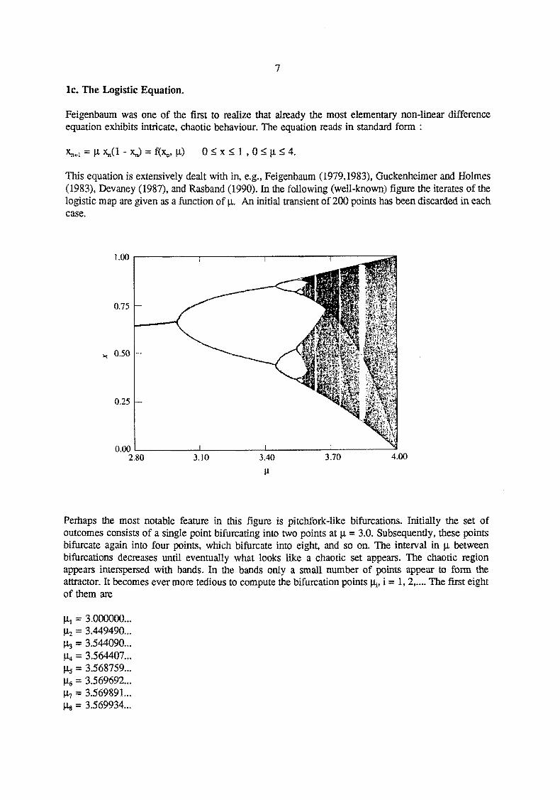
lc. The Logistic Equation.

Feigenbaum was one of the first to realize that already the most elementary non-linear difference equation exhibits intricate, chaotic behaviour. The equation reads in standard form :

This equation is extensively dealt with in, e.g., Feigenbaum (1979, 1983), Guckenheimer and Holmes (1983), Devaney (1987), and Rasband (1990). In the following (well-known) figure the iterates of the logistic map are given as a function of 11· An initial transient of 200 points has been discarded in each case.

0.75

~ 0.50

0.25

0.00 ~..._ ____ .~,._ ____ ..J.._ ____ --L-____ __.:;a

2.80 3.10 3.40 3.70 4.00

ll

Perhaps the most notable feature in this figure is pitchfork-like bifurcations. Initially the set of outcomes consists of a single point bifurcating into two points at J.1 = 3.0. Subsequently, these points bifurcate again into four points, which bifurcate into eight, and so on. The interval in J.1 between bifurcations decreases until eventually what looks like a chaotic set appears. The chaotic region appears interspersed with bands. In the bands only a small number of points appear to form the attractor. It becomes ever more tedious to compute the bifurcation points IJ.i, i = 1, 2, .... The first eight of them are

111 = 3.000000 .. . ~ = 3.449490 .. . 113 = 3.544090 ... 114 = 3.564407 .. . J.1s = 3.568759 .. . J.16 = 3.569692 ... 1-17 = 3.569891... Jls = 3.569934 ...

8

We observe a rapid convergence, which seems to be geometric. This is indeed the case. Numerical experiments yield that the converged value is given by J..l.- = 3.5699456 ..... Further it is found that the quotient

approaches in the limit n ~ oo the value

0 = 4.6692016091.. ..

The logistic map reveals universal behaviour :

a. The phenomenon of period-doubling sterns from the fact that f has no unique inverse. All non­invertible functions f give rise to similar behaviour. The value of the convergence parameter b depends on the character of the maximum. All quadratic maxima leads to the o-value given above. Maxima of different order yield other values for o.

b. Other types of universal behaviour concerning scaling are dealt with in Feigenbaum (1979,1983) and nearly all books on chaos.

Link with fractal dimension.

In the period doubling plot a vertical cut is applied at a I! value for which the system is in a chaotic mode, the set of iterates has a fractal dimension smaller than one. Here we meet with a strange attractor.

9

2. DYNAMICAL SYSTEMS FOR T ~ oo.

Dynamical systems are characterized by a state vector x e Rn. The state is specified at an initial time, t = 0 say, and evolves in time. In the continuous time case x(t) depends continuously on t In the discrete time case x is observed only at discrete time points fn. We then write xn = x(tn). The evolution of the state is governed either by a differential equation or by a difference equation. The corresponding n-dimensional vector fields f usually depend on an m-dimensional parameter vector, say J..L e Rm. Dynamical systems have the fonn of an initial value problem. We only consider autonomous systems, for which f does not explicitly depend on t.

In the discrete time case we have :

Xn+l = f(Xn. Jl) Xn=O = Xo '

and in the continuous time case :

dx/dt = f(x, Jl) x(O) = Xo

The solutions of f(x,Jl) = 0 are called stationary or fixed points. For convenience we assume in the following that the solutions (Xn, n = 0, 1, ... } or {x(t), t ~ 0} are bounded for all starting values Xo and all parameter values Jl. We might also assume that we study only those Combinations of starting and parameter values, for which the solution remains bounded for n ~ = or t ~ oo.

In the following we introduce some properties for the continous time case. They can be easily translated to the discrete time case.

The dynamics of the system is governed by the vector field f in the equations above. When the systen evolves in time, x(t) follows a path in phase space Rn. Other words used to denote this path are : evolution, trajectory, orbit, motion. Stationary points are special (static) evolutions. We may choose each point in Rn as starting value Xo and observe the paths of the corresponding solutions. In the continuous time case all paths together resemble the flow of a fluid. We may describe this flow by a mapping, also called evolution operator :

<1>1 : Rn x R"' ~ Rn , defmed by <I>lXo) = x(t)

In 2-d we may sketch this as follows :

The operator <1>1 has the properties :

1. <I>t.,()(Xo) = Xo 2. <I>l<I>t'(Xo)) = <I>t+t•(Xo) = x(t + t') 3. <I>1(Xo) is continuous in t and Xo

x,

10

For continuous time systems the inverse of cl> nearly always exists because initial value problems have unique solutions under very mild conditions on f. For discrete time systems the evolution operator may be non-invertible.

2a. Conservative Systems.

We call a system conservative if cl>t preserves volume in phase space Rn. In terms of fluid dynamics we have to do with an incompressible flow in Rn. In formula:

{cl>t(Xo) I Xo E A} =A for all subsets A of Rn and t;;::: 0.

So, for fixed t ;;::: 0, cl>t is a one-to-one mapping of Rn onto Rn.

Example : Harmonic oscillator.

Consider a mass m attracted to the origin by a force proportional to its distance from the origin. Tile constant of proportionality is denoted by k. A one-dimensional sketch is :

----------·-'?

7=-:Jx ---- <

The second law of Newton states : m d2x 1 df= - kx. We write this second order ODE in standard form defining :

---7

X1 :S X

x2 = dx/dt

So, the phase space is 2-dimensional, and the initial value problem reads :

dxl/dt = Xz dXzldt = - of- xl

The general solution is x1(t) = c1 cos(rot) + Cz sin(rot), xz(t) = -c1 ro sin(rot) + Cz ro cos(rot),

with ro = ..J k/m, and the constants c1 and Cz determined by the initial conditions. Sketch of the orbits in phase space :

•

11

2b. Dissipative Systems.

A system is called dissipative if it contracts volume in phase space. Let us define an attracting set X by: For an aselect choice of Xo e Rn <I>t (Xo) approaches X, for t ~ oo, with positive chance. In a careless formulation :

under the exclusion of some extraordinary points Xo· The behaviour of <I>t(Xo) before reaching the near vicinity of X is called the transient of the evolution.

In case of dissipative systems X is smaller than Rn. An attracting set X may consists of several minimal attracting sets or attractors. The precise definition of minimal attracting set is quite subtle and omitted here.

2bl. Point attractors.

Example : Damped harmonic oscillator.

We add friction to the model in the example in §2a. If we take the friction proportional to the velocity, Newton's second law reads :

In standard form : dxtfdt = x2

dxJdt = - ro2x1 - (y/m)x2

All solutions now spiral to the origin. We omit the explicitly known solutions and sketch the general behaviour for small y :

.,. ·5 10

• In this example the attracting set X consists of one point, a point attractor. In other cases X may consist of more separate points, each having its own basin of attraction. Point attractors are fixed points, but not all fixed points are attracting. The basins of attraction may have a very complicated

12

structure and fmctal dimension.

Example : Damped pendulum under influence of two attracting forces.

Consider a one-dimensional pendulum. It is under the influence of two attracting forces, e.g., because the pendulum is positively charged, while two negative charges are placed aside of the pendulum pa1h. The forces decrease with increasing distance.

I

I I

I t I

/ ,;

-,-

' ' \ \

' \ J I I

I I

/

This system has one position variable, the angle 8. The 2-dimensional phase space contains the vectors (8, d9/dt). Because of the friction the initial motion of the pendulum will damp out. The system has 4 stationary points in phase space : two unstable points (1t,O), ( -1t,O), where the forces cancel each other, and two stable ones (91,0), (92,0). The last two points together form an attracting set and each of the points is a point attractor. For a fixed set of parameters (pendulum length, strength of the forces, etc.) one can try to calculate the basins of attmction. This is a hard task because the integmtion is performed with finite accuracy and the boundaries between the basins are no continuous curves. In some regions points of both basins are undiscemible in pmctice. •

2b2. Periodic Attractors.

X is called a periodic attractor if it consists of periodic solutions. An attracting set consisting of one periodic solution is usually called a limit cycle.

Example : Van der Pol equation.

The famous van der Pol equation is a second order, non-linear ODE :

d2x/df + Jl (x2- 1) dx/dt + x = 0

In standard form this reads : dx1/dt = x2

dxJdt = - x1 - !l(x/ - l)x2

This equation has the origin as fixed point, but this is no element of X. The origin is in this example

13

a point, which we above called extraordinary. All solutions starting outside the origin attract, for 1J. > 0, to a limit cycle. Its fonn depends on the value of IJ.. For ll = 10 we get the following figure :

-10

-15 -,....--rr+,' I. I'. I. t ••• t ,, ' ' '. t' ''I' I It f I. -2.5 -2 -1.5 -1 -8.5 8 3,, 1 1..5 2 2.5

XI

Example: Contracting rotator.

This system is a continuous time variant of the logistic equation in 2-d. The phase space is R2• It is

convenient to use polar coordinates (r,9). The equations are :

dr/dt = ll r (1-r) d9/dt = 1

Due to the second equation the solution will rotate with constant angular velocity around the origin. The solution starting at (r0, 90) is explicitly given by

r(t) = r0 I (r0 - (r0 - l)e-J.U) 9(t) = 90 + t

So, if t.t. > 0 and r0 > 0, the solutions approach, fort~ oo, the unit circle. There they keep circling around. •

2b3. Quasi-periodic Attractors.

X is called quasi periodic if it consists of quasi-periodic solutions. A simple example of a quasi­periodic function is cos (co1t) cos(COzt). If rot and COz are commensurable, that is rotfCOz e Q, then this function is periodic. If the angular velocities ro1 and COz are incommensurable, that is, their quotient is not rational, the funcion is a-periodic.

2b4. Chaotic Attractors.

Chaotic attractors are characterized by the occurence of divergence or sensitive dependence on the initial conditons. Definition : an evolution tt> is sensitive in x if :

a o > 0 exists such that for each e > 0 one can find an initial point x' with I x - x' / < e, but I tl>T(x) - tl>T(x') I > o for some T.

14

In other words, in each vicinity of x, however small it may be, a solution starts that diverges from the solution starting in x itself.

Remarks:

1. For the logistic equation ci> is either sensitive in all points of the interval (0, 1 ), or only sensitive in points, that together form a set of (Lebesque) measure zero. It is not known whether a similar property holds in general.

2. Chaotic attractors generally contain a lot of periodic solutions, but these are instable : small perturbations, which are unavoidably present in numerical calculations, lead to deviation from such a solution. Furthermore, if we choose a point of X arbitrarily, we have a vanishing chance to find an element of a periodic solution.

Example : Doubling mapping.

The doubling mapping is a one-dimensional, discrete time system defined by

~+1 = 2~ (modulo 1) = f(xJ

So, for all n we have~£ [0,1]. The iteration function f(x) looks like

1

0.a

0.6

X:

L..

0.4

0.2

II 0 0.2 0.4 0.6 a.a 1

)(

An alternative representation makes use of the unit circle as domain and range. Points on this circle are specified by the angle 9 :

The difference equation then reads : en+!= 29n mod(21t).

15

The divergence in this system is clearly observed. The n-th iterate of the mapping is given by

F(Xo) = 2~ (modulo 1)

So, small differences are always blown up. The dynamics of this system has many interesting features. All points of the form Xo = 1 I 2n are attracted to x = 0. There are periodic solutions with a period length of n iterations, the so-called n­cycles, for all n EN. All initial values are sensitive. These properties are most conveniently concluded from symbolic dynamics. Let us write the initial value Xo in binary representation :

with the ~ equal to 0 or 1.

Application of f yields a shift of all the a; one position to the left :

and in general

If only n digits of Xo are specified, the n-th and higher iterates will contain not any infonnation from Xo· We also immediately see that the periodic solutions just correspond to those Xo that have periodic binary representations. The rational numbers Q have (binary) representations with periodic tails. So, evolutions starting at a rational number are attracted to periodic solutions.

Remark : The dynamics of the doubling mapping on the unit interval or circle is conservative and chaotic. The system illustrates sensitivity to initial conditions; it does not show attraction to a strange attractor. •

2b5. Structure of Chaotic Attractors.

Let us focus on dissipative, continuous time systems. We assume the presence of an attractor, which is in nearly all points sensitive and thus shows divergence nearly everywhere. The uniqueness theorem forbids that solutions will cross. This implies that such a bounded subset of the phase space must have a very complicated structure. For example, the surface of a sphere (2-dimensional) in R3 will not suffice, because the solutions must have the possibility to pass each other. The dimension of the attractor must essentially be larger than 2. So, continuous time systems of order 1 and 2 can not have strange attractors. For discrete time systems it is otherwise, because there the uniqueness theorem does not apply.

Strange attractors often possess a layered structure. Then they seem to be produced in the same way as pie dough, namely by stretching and folding. The stretching corresponds to divergence and the folding is necessary to keep the solutions within a bounded volume. Such objects usually have fractal dimension.

It may also occur that the divergence is quite small everywhere on the attractor except for a relatively small region. As an example we refer to the 'butterfly' attractor of the Lorentz system dealt with in § 1. This object has dimension a bit larger than 2. The wings are nearly 2-dimensional. The necessary crossings of the orbits take place where the wings overlap

16

3. FRACTAL DIMENSION.

Hausdorff introduced a generalization of the classical notion of dimension already in 1917. The study of the detailed structure of irregularly shaped objects like clouds and rocky coastlines led Mandelbrot (1967) to a reconsideration of the concept of dimension. The relevance of these ideas did not become fully clear before chaos theory was developed. The famous books by Mandelbrot (1977,1982) and the visualization of his ideas by Peitgen and Richter (1986) strongly pushed the common acceptance of the concept of fractal dimension.

Let us start by remarking that many definitions of generalized dimension are in use. The one closest to intuition is capacity rlcap· We study an object X in Rn. The capacity is given in terms of coverings with non-overlapping, n-dimensional boxes with all edges of equal length 1. Let, for given 1 > 0, N(l) be the minimal number of such boxes necessary to cover X. For 1 .!. 0 we have the scaling relation

N(l) - rd..,.

where dcap is defined as

d = - lim In N([) cap IJ.O In/

This definition is not very general, because the limit does not always exist. The Hausdorff dimension, which can be seen as a refinement of dcap• circumvents this problem, but will not be dealt with here.

In other dimension definitions the contributions from different regions of X are not weighted equally. The weighting is introduced via a measure on X. Dynamical systems that organize themselves on an attractor X in phase space induce a measure on X in a natural way. If X is covered with boxes, an evolution of the system on X will, fort~ oo, not visit each box with the same frequency. The ratio's of these frequencies induce, after normalization, a measure or probability distribution on the covering, and , in the limit 1 .!. 0, on X itself. Because one particular evolution is used, the result will formally depend on the initial value of that evolution. In practice this dependence is not relevant if X has chaotic dynamics, because then it is impossible to follow one evolution exactly. Even if one starts at one of the points of a periodic solution, the numerical inaccuracy will cause that this (instable) solution will be left. Let us denote the measure of box i by Pi· It gives the chance to find the system in box i if observed at an arbitrary time. If the measure is uniform over X we, of course, have

In the limit 1 .!. 0 the discrete measure p1 transfonns into a continuous measure Px on X. A commonly used definition based on a measure is the correlation dimension dcor introduced by Grassberger and Procaccia (1983a,b). We cover X with boxes of equal size I and choose that covering for which the correlation function

is minimal. Pil) may be interpreted as the chance that two arbitrary selected points belong to the same box, i.e., have a distance smaller than or equal to I. dcor is defined by

17

from which we have the scaling relation

This idea is generalized by, amongst others, Hentschel and Procaccia (1984). They introduced the q­fold correlation function Pq by

Here, q may attain all positive real values. The generalized dimensions Dq are defined by

D =lim _I_ In P,p) q I.!. 0 q-1 In I

Special case are 0 0 = dcap and 0 2 = <ioor· D1 is called the information dimension. All the Dq together characterize the scaling properties of X.

3a. Numerical Estimation of dup•

In practice only a finite number of points {x;, i = 1, .. , M} on X is given. They often stem from measurements. It is assumed that these points represent X appropriately. That means that the density of points is highest in the regions mostly visited by the evolutions. dcap is estimated by covering the set of points X; with boxes of linear size L N(l) is approximated by :

N'(l) : the number of boxes containing at least one of the X;.

This procedure is called box-counting. The values N'(l) are determined for a range of 1 values. Next, In N(l) is plotted against In l. In the ideal situation this plot yields a straight line. Its slope is the value of dcor· The application of the method meets with several problems in practice :

- It has no sense to take 1 smaller than the smallest distance between the X;, so the limit 1 J. 0 can only be approximated. It often appears that the plot of ln N'(l) against In 1 is a straight line only in a small 1 interval.

-The X; are given with finite accuracy. This also puts a lower bound on the range of L - The number of necessary boxes may increase very fast. For example, if X is an object in R3 with

maximum linear size about L, a reasonable covering could start with boxes of size L /5. The number of boxes is then 53 = 125. It is common to reduce the box size by a factor of 2 to obtain a second covering. This enhances the number of boxes to 1000. Another halving of the box size leads to a covering consisting of 8000 boxes. Such a fine mesh makes only sense, if M is in the same order of magnitude. So, to obtain three point in the log-log plot X should be known in about 8000 points. And so on. This makes clear that the method is hardly applicable in higher dimensions.

•

18

3b. Numerical Estimation of d.eor•

As indicated above, P2 can be approximated by

P2 '(1) = {number of distances between the xi smaller than or equal to 1} I (M(M-1))

So, one has to determine the distances between the given points Xj. The number of distances is M(M- 1), which can be quite large, but it is clear that in fact only distances between neighbouring points are relevant in view of the limit 1 ..L. 0. An efficient algorithm is proposed by Theiler (1987); it avoids unnecessary distance calculations. Note, that if the (relevant) distances have been determined once and for all, they can be ordered with respect to magnitude. The determination ofP2'(1) for alll is then quite easy and costs hardly any time.

Example: Correlation dimension of the Lorentz attractor.

We integrate the Lorenz model and obtain M discrete 3-dimensional points xi by xi= x(iot), with ot a fixed time interval. An evolution circles around one of the wings of the butterfly in a time interval oflengt about T = 0.3, and we take ot = T /10. Transient points are omitted. The slope of the log-log plot forM= 1000 yields dimension estimated= 2.1 :

CORRELATION FUNCTION P2(LJ

10-3 .-------------------------------~-------.

..J 10-4

N 0..

z 0 ...... 1-u z ::l I....

z 0 ...... 1-<I: ..J 10-s w 0! 0! 0 u

10-6 ~----~--~~~~~~----~--~~~-..-.r 10°

19

3c. Noise.

In the example in § 3b the data are not corrupted by noise as is the case in most measurements. The noise adds a stochastic element to the data. If the data would have been produced completely stochastically, the log-log plots would show a straight line with slope the dimension of the system, thus slope n if the system lives in Rn. Small amplitude noise has the effect that the slope in the log-log plot is equal to n for small 1 values, whereas for higher 1 values a smaller slope is observed corresponding to dcor or dcap·

3d. Dimension Estimation and Principal Component Analysis.

The numerical procedures for dimension estimation may require a lot of computer time. Considerable improvement can be reached if insights from statistical analysis are applied. Albano et al. (1988) propose to use principal component analysis. We shall explain this interesting idea in short :

The n-dimensional points Xj , i = 1, ... , M, contain the information about X. It has advantages to use as origin the centre of mass Xo of these points defined by

We apply the translation xi~ xi- :xo. so that the xi are given with respect to Xo· After that the xi are arranged in an M*n matrix A :

A= 1

1M

Let us consider the points Xj as being M realizations of an n-dimensional probability distribution. The n*n matrix AT A is then just the (unnormalized) correlation matrix of this distribution. The off-diagonal elements give an indication of the redundancy in the data. The eigenvectors of AT A are called the principal components of the data set. The eigenvalues measure the relative importance of the principal components. These eigenvectors and eigenvalues are most effectively obtained by applying singular value decomposition of A. We may always write

A= UDVT

with

U : an M*n matrix with orthogonal columns. D : an m-dimensional diagonal matrix with on the diagonal the square roots of the eigenvalues (also

called 'singular values') of AT A. The singular values are ordered from large (D1) to small (Dm). V : an m *m orthogonal matrix; its columns are the eigenvectors of AT A.

If some singular values are relatively small, the corresponding eigenvectors, or principal axes, are ignored. This removes the redundancy in the data. For example, if Di I D1 << 1 fori;::: 2, only the first principal axis is important : the set X is apparently !-dimensional.

20

These insights are used as follows. We project the points xi onto the principal axes by

A' =AU.

Let us assume that for some n' < n the Di are very small if j > n'. As criterion we could take that Di I D1 ~ 104

, j > n'. Then, the columns n'+l, ... , n of A' may be ignored. The reduced matrx A" has thus size M*n', and contains essentially the same information as the original matrix A. So, we may use A'' instead of A in the estimation procedures. This will not only save a lot of computer time, but the reduction appears to be also favourable to the stability of the estimation procedure.

21

4. LY APUNOV EXPONENTS.

The Lyapunov exponents (LE) ~ , i = 1, .. , n, of an n-dimensional system give an indication of the strength of the divergence (if any) on X. The sum of the i largest ~ is a measure for the magnification of an arbitrarily chosen i-dimensional volume while it evolves in time. For example, if A.1 is positive, the length of intervals will on average be stretched. The dynamics on X is then called chaotic and X is called a strange attmctor.

Let us first give a geometrical introduction of the LE's. We start with an-dimensional sphere and follow its evolution. Initially the sphere will defonn into an ellipsoid. It suffices to follow the principal axes of this ellipsoid, which are initially orthogonal. If the system is chaotic, at least one of the principal axes will be stretched. Other axes will reduce in length. Let us order the axes Pi(t) according to their stretching rate. For t > 0 the axes will no longer remain orthogonal in generaL We shall generally observe that the angles between the main principal axis p1 and the other Pi (t), i = 2, .. , n, are decreasing. A possible (geometric) definition of the LE's is :

A.;= lim~ lnjp;(t)j I->~ f

In the present context we restrict our attention to the largest LE ~ and to discrete time systems. The numerical approach in the continuous time case is quite analogous. See, e.g. Wolf et al. (1985).

4a. ~ for One-dimensional Systems.

We follow an evolution Xn.r1 = f(xJ starting at Xo and are interested in the behaviour of small intervals around Xo· Let us look at the interval [J<o, Xo + Eol After one itemtion the interval length has changed from ! Eo I into I E1 I and is approximately given by

At the next itemtion again a contmction or magnification takes place :

Repeated application of this procedure yields after n iterations an interval length En given by

This approximation holds even for large n if we take at the same time the limit Eo -L 0. It is convenient to write

I J'(x;) I 5 em(x)

Ifm(xi) > 0 (< 0) the interval is stretched (squeezed) at the i-th iteration. With this definition we may write

A.1 is defined as the average of the m(x) in the limit n ~ oo :

22

1 n-1

1 n-1

A1(x0) = lim - E m(x) "" lim - l':lnl f(x)l n -+- n i=l n -+- n i:l

The LE defined this way depends on Xo because the average is taken over the specific evolution starting at Xo· However, in practice this dependence is nearly always negligible. Note, that different regions may contribute differently to A1• First, because the value of f will vary over X, and second, because the evolution will not visit each region with the same frequency. In tenns of the measure Px introduced in §3 we may also write

A1 = J m(x) dp" X

If A1 > 0 intervals will on average be stretched by a factor of exp(A1n) until their size is of the same order as the diameter of the attractor itself. Meanwhile they will probably be folded. We see that the points of an arbitrary small interval get in the long run scattered over the whole attractor.

Example : Doubling mapping.

Because for this mapping f = 2, we have A1 = ln 2. •

The definition of the LE's above makes use of the base e. This example suggests that it makes sense to introduce a slightly alternative LE, namely with respect to base 2. We then write

'II = AI _, "'t- -ln2

e"' = 2~

The growth of interval length is thus given by 2 ** (A1 'n). In the computer the initial value Xo is stored in binary representation with a certain number of digits, say flo. Upon iteration the uncertainty in the successive xi, i = 1, 2, .. will grow. After about (1 I A1') iterations the last bit of Xn will no longer contain information specified in :xo. After (no I A1 ') iterations all information contained in Xo has got lost. Therefore, A1' is expressed in units of bits per iteration.

For example, assume that no= 32, so figures are stored with decimal accuracy of about 10·10• The

doubling mapping has A1' = 1, so after 32 iterations the outcomes are completely uncertain.

4b. A1 for n-dimensional Systems.

Analogous to the one-dimensional case, we take an interval [Xo. Xo + f.o]. Note, that this interval now has an orientation with respect to Xo specified by the direction of f.o. After one iteration the length I f-o I of the vector f-o is approximately given by

I e1 I = I f(xo + eo) - f(Xo) I = I J(xo) * eo I

with J(Xo) the n*n Jacobian matrix off evaluated at Xo· Repeating the iterations we get

I €n I = I J(xn-1) * ...... * J(Xo) * eo I

The definition of A1 reads :

23

'l 1' 1 In le,.l 1' 1 In I l 1\.1 = 1m _ -r;:-r = 1m _ e,.

,. ..... ~ n leol ,. ....... n

This definition is easily interpreted in the following two cases :

Example : J is constant.

Then we have

Let us denote the eigenvectors of J by 'J...1';;:: 'A.z';;:: ... ;;:: An' with corresponding eigenvectors e1, ez, ... , ~- If we choose eo along one of the ei, we will find that definition (*) just yields ln('J.../). However, in general eo can be expressed as a linear combination of the ei :

Because

So,defmition (*) wil in general yield the largest LE 'J...1 = ln 'J...1' •

Example : The orbit is periodic, say an m-cycle.

In this case we have

I fn•m I= I An Eo I with A= J(Xro.t) * ....... * J(Xo).

The A; are given by the logarithm of the eigenvalues of the Jacobian matrix A of the cycle. •

4c. Numerical Calculation of 'J...1•

4cl. Calculation of ~ from Model Calculations.

If the vector field f of the system is known, definition (*) can be applied directly. Because f, and thus J, are known everywhere on X, the algorithm to calculate ~ is quite straightforward. For arbitrarily chosen Xo and eo we evaluate the system

Xn+l = f(xJ fn+l = J(Xn)fn.

for n = 1, 2, ... , meanwhile observing the behaviour of

as a function of n. This naive approach will certainly lead to computer overflow. The problem can be circumvented by nonnalizing. We take I eo I = 1, and nonnalize after each iteration step the interval length to unity. If we denote the interval length before nonnalizing by I t:n' I , we have that

So, in practice we may use the fonnula

which behaves numerically well.

Example : Henon mapping.

The Henon mapping is given by

The Jacobian J(x,y) is

[ -2ax lJ

J(x,y) = b 0

24

Xn .. t = 1 - aXn2 + Yn Yn+l = bXn

= ft(Xn, Yn) = fiXn• YJ

Plot of the pairs (Xn,yJ, n = 10, .... , 2000 for a= 1.4, b = 0.3, and arbitrary inital values :

0.3

0.2

0.1

0

-11.1

-0.2

-0.3

Plot of At(n) as a function of n ; _,_,

-0 ,4,+-,....,...........+~...-.-t-r-,_,.-.-+-,.-.--,-,-t...,....,...,...,.+-,-..,..,..~1.= -1.5 -1 -0.5 0 0.5 J

X

0.54·-r----------------,

0.52

0.5-

• 0

"42

0 200 400 600 800 1£3 1209 1400 1600 1809 2E3

N

25

4c2. Estimation of "-t from Data.

In practice f is often not known, but one has at one's disposal only an evolution {X;, i = 1, 2, .... }. Here, then-dimensional vectors X; represent the complete state. In §5 we shall deal with the case that the data contains only partial infonnation about the state of the system.

A numerical estimation of "-t can be obtained as follows. We search in the series for the point xJ closest to Xo· The number of iteration steps between the two points may not be too small, because the evolution must in the mean time have visited at least some other regions of X. Following the series starting at Xo and xi respectively, we calculate the distances

I En I = I xj+n - "" I , n = o,1,2 •....

If En becomes too large, i.e. in the order of a fraction of the size of X, the direction of xj+n - Xu is nonnalized. This means that K.i+n is replaced by, say, xk, which is closer to Xu but has the same direction with respect to Xu· Because the series contains a finite number of points, one cannot hope to find a replacement vector that falls exactly along the line segment specified by the vector K.i+n - Xu. but we can look for a point that comes close. The procedure is described by Wolf et al. (1985), who also give relevant computer programs. The method leads to reasonable values of A.1 provided that enough data is available. In principle the method also applies to the detennination of the other non-negative A.'s, but it appears in practice that the amount of data must be very large, so that the time needed for neighbour searching becomes inacceptibly long. Negative A.'s can not at all be calculated this way, because they correspond to directions which collapse exponentially fast.

26

S. THE RECONSTRUCTION PROBLEM.

In many practical situations no appropriate model for the system under consideration is known. One does often not know the phase space variables needed to fully describe the dynamics, and even the number of the relevant degrees of freedom is often uncertain. Only measurements are available. One would like to have at one's disposal measurements of the complete state vector x = (x1, x2 , ••••••• ).In practice only one or a few components are measured. The measured quantity is referred to as the read­out function. We shall denote it by x(t). In general xis a function of all state variables, so x(t) = x(xlt), x2(t) , ...... ). How could one determine properties of the complete system, and in particular of the (possible) attractor, from these incomplete data ? There is fortunately a partial answer to this question. The standard references are Packard et al. (1980) and Takens (1981). We call this approach reconstruction.

Illustration : The idea behind the reconstruction method is easy to illustrate in the simple case of a one-dimensional mechanical system, e.g., a pendulum. The phase space variables of such a system are the position variable x and the impuls (velocity) variable dx/dt. Complete knowledge of the evolution of the system implies that the points (x,dx/dt) are known as functions of time t.

Let us assume that only position measurements xi= x(t) at discrete time points~= to + iot are available with ot a fixed time interval. Then, the differences (xi+I - xi) I ot are approximations for the velocities dx/dt at t = fi. In other words, the series xi, i = 1, 2, ... indeed contains (approximate) knowledge about the trajectory in phase-space. •

The key idea is to embed the scalar series { ~} into a higher dimensional space with dimension de, say. First we have to choose an embedding dimension de £ N and a delay k £ N. Then, we construct a series of de-dimensional vectors by the procedure :

Yo = (Xo, Xo ... k• Xo ... 2k ........ , Xo+<:~, .. J Yt = (xl' x, ... k' xt ... 2k•··· ..... , xt+<~ •• J Y2 = (:t:z. Xz ... k' x2 ... 2k' ......... , x2 ... d,•k)

etcetera.

The points {yi, i = 1, 2, .. } lie on an artificial attractor Yin the artificial de-dimensional phase space, and perform there evolutions. A very important observation is (see the references mentioned above), that the dynamics on Y has the same characteristics as the dynamics on X. For example, X and Y have identical dimensions and Lyapunov exponents.

Sa. Estimation of the Embedding Dimension.

In practice ~ is not known in advance. To estimate a reliable value for de one applies the embedding procedure for increasing de values : de = 1, 2, .... For each de value the (capacity or correlation) dimension d ofthe resulting Y is calculated using the techniques in §3. If the procedure saturates, i.e., the estimated dimension d of Y, and thus X, keeps constant when de is enhanced, the minimum embedding dimension has been obtained. The theoretical upper bound on de is given by de = 2d + 1. Saturation is often found at much smaller de values.

27

Sb. Estimation of Delay k.

The choice of k is not very critical. The value of the time interval kot should not too small, because then the components of the y1 are nearly identical. If kot is too large, i.e., much larger than the infonnation decay time detennined by the largest Lyapunov exponent, then there is no dynamical correlation between the points.

Sc. Remarks on Reconstruction.

- Let us, in contrast with chaotic systems, investigate what will happen if the time series under consideration has been generated by a stochastic process. Then, no finite-dimensional mechanism exists which could have produced the (infinitely long) series. We may conclude that no saturation will take place when we apply the reconstruction technique to a really stochastic series.

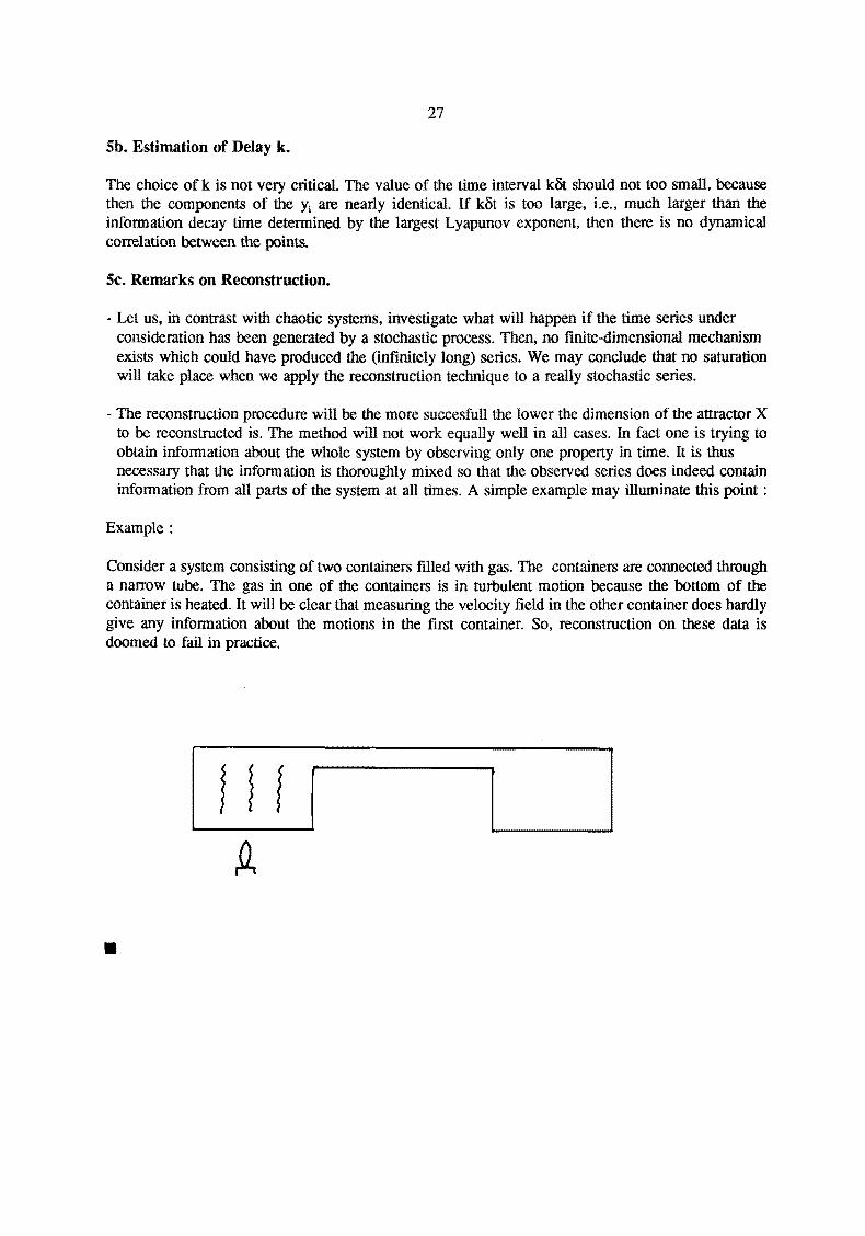
- The reconstruction procedure will be the more succesfull the lower the dimension of the attractor X to be reconstructed is. The method will not work equally well in all cases. In fact one is trying to obtain infonnation about the whole system by observing only one property in time. It is thus necessary that the information is thoroughly mixed so that the observed series does indeed contain infonnation from all parts of the system at all times. A simple example may illuminate this point :

Example:

Consider a system consisting of two containers filled with gas. The containers are connected through a narrow tube. The gas in one of the containers is in turbulent motion because the bottom of the container is heated. It will be clear that measuring the velocity field in the other container does hardly give any infonnation about the motions in the first container. So, reconstruction on these data is doomed to fail in practice .

•

28

Example : Reconstruction of the Lorenz model data.

We use as data 2500 calculated values of the x1 component of an evolution on the Lorenz attractor. For d, > 3 the slope d of the log-log plot saturates. However, the value of d "" 2.3 is higher than the real value d "" 2.1. From this we conclude that the time series used is still too short. The estimates have always to be checked on the dependence on the amount of data.

•

_J

N 0..

10-3~----------------------------------------~

L

De = 1 De = 2 De = 3 De = 4 De = 5 De = 6

29

6. PREDICTION.

In the present context we restrict our attention to dissipative, chaotic systems. The evolutions of these systems take, in the long run, place on an chaotic ('strange') attractor X. Due to the divergence of the evolutions, the behaviour of these deterministic systems is in the long run unpredictable. Another way to express this property is to call those systems 'sensitive to the initial conditions'. Because of the loss of information, small uncertainties, e.g., errors in the initial conditions, will exponentially grow in time on the average. However, thanks to the determinism of the sytems prediction is not impossible, but it makes only sense if performed within a certain time horizon. In §6a we shall shortly dwell on the predicting behaviour of systems of which the model is fully known. However, in practice one often has no (or only an incomplete) model of the system, but only measurements of some property of the system are available. Here, we are mostly interested how the measured time series can be extrapolated. This is the subject of §6b.

6a. Prediction through Model Calculations.

Let us assume that we have available a reliable model, i.e., a set of differential or difference equations. Given the initial state it is a matter of numerical technique to calculate the solution as time evolves. The 'loss rate' of the system is measured by the largest Lyapunov exponent~. as explained in §4. We emphasize that A.-1 is a measure of the average divergence of evolutions on X. Local divergences may considerably differ from the average value.

Example : Lorentz attractor.

The Lorentz model is already presented in § 1. Its attractor is the well-known butterfly :

40

35

30

~ 25

20

15

10

-5 0

X1

The parameter set used is (cr,b,r) = (10,8/3,28).

' ...

5 10 15 20

30

The picture suggests that the divergence in the wings is very small, except for the central region where the wings overlap. From §4 we know that the local stretching at a point x E X is determined by the largest eigenvalue of the Jacobian J(x). For the Lorentz model we have

A point at the outer side of one of the wings is x1 = (17.1, 20.5, 35.7). The corresponding eigenvalues of J(x1) are : (0.8 + 20.8i, 0.8 - 20.8i, -15.3). A point in the central, 'chaotic' region of the attractor is x2 = (1.7, 1.0, 20.8). The corresponding eigenvalues of J(x~ are : (3.6, -2.2, -15.1).

The strongly negative eigenvalues indicate that orbits starting outside the attractor are very fast attracted to the attractor. This takes place along the corresponding eigenvectors which are everywhere perpendicular to the wings. The positivity of (the real part of) the largest eigenvalues corresponds to the stretching inside the attractor. At x1 the divergence is very small, whereas at x2 a considerable divergence is observed. As long as evolutions are in the 'quiet' regions of the wings, predictions may be very reliable. If an evolution passes the 'chaotic' region a sudden loss of information takes place. This deteriorates the reliability of the prediction of such an evolution considerably.

6b. Prediction (Extrapolation) of a Chaotic Time Series.

6bl. One-step-ahead Prediction.

Let us first deal with one-step-ahead prediction. We consider a time series {xi, i = 1, ... , M} representing some property of a dissipative, chaotic system. The xi are measured at equidistant time points to+ i<3t. We shall outline a procedure to get an estimate for xM+I· This procedure is based on finding local portions of the time series in the past, which closely resemble the present, and basing the predictions on what occurred immediately after these past events. It should be emphasized that no attempt is made to fit a function to the whole time series at once. The approach can quite simply be automated and may give striking results, if the attractor dimension is not too high and enough data is available. The procedure can be summarized as follows :

1. Apply reconstruction. The procedure dealt with in §5 will yield the embedding dimension de E N and the (fractal) dimension d of X. Meanwhile the scalar series {xi, i = 1, ... , M} is transformed into a series {Yi• i = 1, .... , M'} of de-dimensional vectors with M' = M - (de - 1). The problem is now to estimate YM'+l·

2. Search neighbours of YM· in the series {yJ.

3. Find the evolution of these neighbours after one iteration.

4. Fit a (linear, quadratic, cubic, or .... ) mapping to the one-step-ahead evolutions of the neighbours.

5. Apply this map to YM'. This yields an estimate for YM'+I• and the last element of YM'+I is an estimate for xM+I·

We shall explain these points in more detail :

31

ad 1 : The reconstruction procedure will only be succesfull if

- the system is dissipative and chaotic; then the evolutions lie on a chaotic attractor X - the dimension of X is low - enough data is available.

ad 2 : For practical reasons one usually fixes the number of neighbours sought for. It would probably be better to select all neighbouring points within a sphere with given radius around YM'·

ad 3 and 4: To illustrate the fitting procedure we shall write it out for a linear mapping. In Farmer and Sidorowich (1987) it is reported that higher order fitting does not always lead to appreciably better results. For notational ease we shall write m = de.

Let p1, p2, ••• , Pn be the set of n m-dimensional neighbouring vectors of YM'· After one iteration these vectors have evolved into the vectors q1, ~ •••••.. , ~· The q-vectors are easily obtained from the p­vectors. For example, if some p-vector is given by

then the corresponding q-vector is given by

A linear mapping of them-dimensional space into itself is given by a m*m matrix A and an m-dimensional vector b. Because it maps Pi unto qi, i = 1, .. , n, it satisfies :

Api + b = qi, i = 1, ... ,n.

It is convenient to introduce an (m+ 1 )*n matrix P by

Pt,t P2,1 Pn,l

Pt;J. P2;1.

P=

Pt,m P2,m Pn,m

1 1 1

where Pt,i is the i-th element of vector p1, etc .. We also specify an m*(m+1) matrix A' by

at,t at;J. at.m bl

a2.1 a2;J. a2.m b2

A'=

am,l am). am,m bm

32

Then, the system of n linear equations can be written as

A'P=Q

with the (m*n) matrix Q given by

Q:;;

This system contains m*n equations and m*(m+ 1) unknowns. For n = m+ 1 a unique solution exists provided that P is not singular. For n > m+ 1 the system can be solved in the least squares sense. A convenient approach makes use of singular value decomposition, in which the matrix pT is decomposed as

pT::::: u D yT

with

U: an n*(m+1) matrix with orthogonal columns, so UTU equals the (m+l)*(m+l) unit matrix. D : an (m+ I)-dimensional diagonal matrix with on the diagonal the square roots of the eigenvalues

(also called the 'singular values') of the (m+ l)*(m+ 1) matrix ppT ordered from large to small. V : an (m+ l)*(m+ 1) orthogonal matrix, so v·1 = VT; its columns are the eigenvectors of PPT.

The singular values that are close to zero are omitted together with the corresponding rows and columns of U and V. After this decomposition and truncation A' follows directly from

Ad 5 : Having estimated A' we have obtained estimates for A and b. The one-step-ahead prediction of the y-series is then given by

YM'+l ::::: AyM' + b.

The one-step-ahead prediction of the x-series follows directly, because it is the last element of YM'+I·

33

6b2. Multiple-step Prediction.

To obtain estimates for xM+i , i = 2, 3, .. , several strategies can be considered :

a. Apply the procedure in steps 1-5 above again, starting with the estimate xM+i·l as the last point of the x-series. For each i a new set of neighbours is sought, from which A and b are recalculated.

b. Modify step 3 in the procedure in §6b1 and determine the evolution of the neighbours after more than one iterations. For example, consider the i-steps-ahead prediction. If p is a neighbour and q its evolution after i steps, we have :

The rest of the procedure is kept unchanged.

c. Calculate A and b using one-step-ahead prediction and apply one and the same (linear) mapping, denoted by L, repeatedly unto YM'· So, if we write

Ay + b = Ly,

then

and xM+i is the last element of YM'+i·

Comments on Prediction Methods a, b, c :

It is clear that method a. makes optimal use of the informatiom in the time series. However, the method is computationally not very attractive. Most of the computer time is namely spent on searching neighbours, and in method a. this search is performed again and again.

This objection does not apply to methods b. and c. It is not directly clear which of the two is preferable. This may depend on the value of i, the order of the fitting mapping, and the amount of data. In Casdagli (1989) some test calculations are discussed.

34

Example : Extrapolation of Lorentz model data.

We take as data a time series of 1000 calculated values of the x1 component of the Lorentz attractor and apply methods b. and c. We use the first 950 data points to estimate values for the rest of the series. Because we have at hand also the real values, we may get an indication of the reliability of these methods. In the plot the calculated values for iteration steps 900-1000 are given, together with the predictions for the interval 950-1000. The dimension de of the embedding space used is 5. the number of neighbours used is 10. The estimates from method b. appear to be quite reliable, whereas the estimates from method c. are much worse and have only predicting power in the restricted interval 950-960.

PREDICTION USING METHOD B

20

15

10

5

X 0

-5

-10

-15

-20 900 920 940 960 960 1E3

INDEX

PREDICTION USING METHOD C

70

r 60

j 50

f 40

i '

30

f X

20 '

10 i 0 t . • -10

-20 900 920 940 960 960 1E3

INDEX

REFERENCES

The references marked with (*) are introductory text books on chaos theory.

ALBANO, A.M., MUENCH, J., SCHWARZ, C., Singular-value decomposition and the Grassberger-Procaccia algorithm, Phys. Rev. A, Vol. 38, nr.6: 3017-3026.

CASDAGLI, M., 1989, Non-linear prediction of chaotic time series, Physica D35: 335-356.

(*) DEVANEY, R.L., 1986, An introduction to chaotic dynamical systems, Addison-Wesley, Menlo Park.

FARMER, J.D., SIDOROWICH, J.J., 1987, Predicting chaotic time series, Phys. Rev. Lett. 59: 845.

FEIGENBAUM, M.J., 1979, The universal properties of non-linear transformations, J. Stat Phys. 21: 669.

FEIGENBAUM, M.J., 1983, Universal behavior in non-linear systems, Physica D7: 16-39.

GLEICK, J., 1987, Chaos,· making a new science, Viking, New York.

GRASSBERGER, P., PROCACCIA, I., 1983a, Characterization of strange attractors, Phys. Rev. Lett. 50: 346-349.

GRASSBERGER, P., PROCACCIA, I., 1983b, Measuring the strangeness of strange attractors, Physica 9D: 189-208.

(*) GUCKENHEIMER, J., HOLMES, P., 1983, Non-linear oscillations, dynamical systems, and bifurcations of vector fields, AppL Math. Sc. 42, Springer Verlag.

HENTSCHEL, H.G.E., PROCACCIA, I., 1984, Relative diffusion in turbulent media: the fractal dimension of clouds, Phys. Rev. A, 29: 1461-1470.

LORENZ, E.N., 1963, Deterministic non-periodic flow, J. Atmos. Sci. 20: 130. Reprinted in: Bai-Lin, H. (ed.), 1984, Chaos, World Scientific, Singapore.

MANDELBROT, B.B., 1967, How long is the coast of Britain?, Statistical self-similarity and fractional dimension, Science 156: 636-638.

MANDELBROT; B.B., 1977, Fractals: form, chance and dimension, Freeman, San Francisco.

MANDELBROT, B.B., 1982, The fractal geometry of nature, Freeman, San Francisco.

(*) MOON, F.C., 1987, Chaotic vibrations, J. Wiley & Sons, New York.

PACKARD, N.H., CRUTCHFIELD, J.P., FARMER, J.D., SHAW, R.S., 1980, Geometry from the time series, Phys. Rev. Lett. 45: 712.

PEITGEN, H.O., RICHTER, P.H., 1986, The beauty of fractals, Springer Verlag, Berlin, 1986.

(*) RASBAND, S.N., 1990, Chaotic dynamics of nonlinear systems, J. Wiley & Sons, New York.

SHAW, R.S., 1984, The dripping faucet as a model chaotic system, Aerial Press, Santa Cruz.

SPARROW, C., 1982, The Lorenz equations: bifurcations, chaos, and strange attractors, Springer Verlag, Berlin.

TAKENS, F., 1980, Detecting strange attractors in turbulence, in: Dynamical systems and turbulence, Warwick. Lecture Notes in Math 898 (Springer, Berlin, 1981): 336-381.

THEILER, J., 1987, Efficient algorithm for estimating the correlation dimension from a set of discrete points, Phys. Rev. A., Vol. 36, Nr. 9: 4456-4462.

(*) THOMPSON, J.M.T., STEWART, H.B., 1986, Non-linear dynamics and chaos, Wiley­Interscience.

WOLF, A., SWIFT, J.B., SWINNEY, H.L., VASTANO, J.A., 1985, Determining Lyapunov exponents from a time-series, Physica D16: 285.