chap004 lecture
TRANSCRIPT
Basic Marketing – Chapter 6Handout 6-1
Elasticity
Chapter 4
Copyright © 2013 by The McGraw-Hill Companies, Inc. All rights reserved.McGraw-Hill/Irwin
4-2
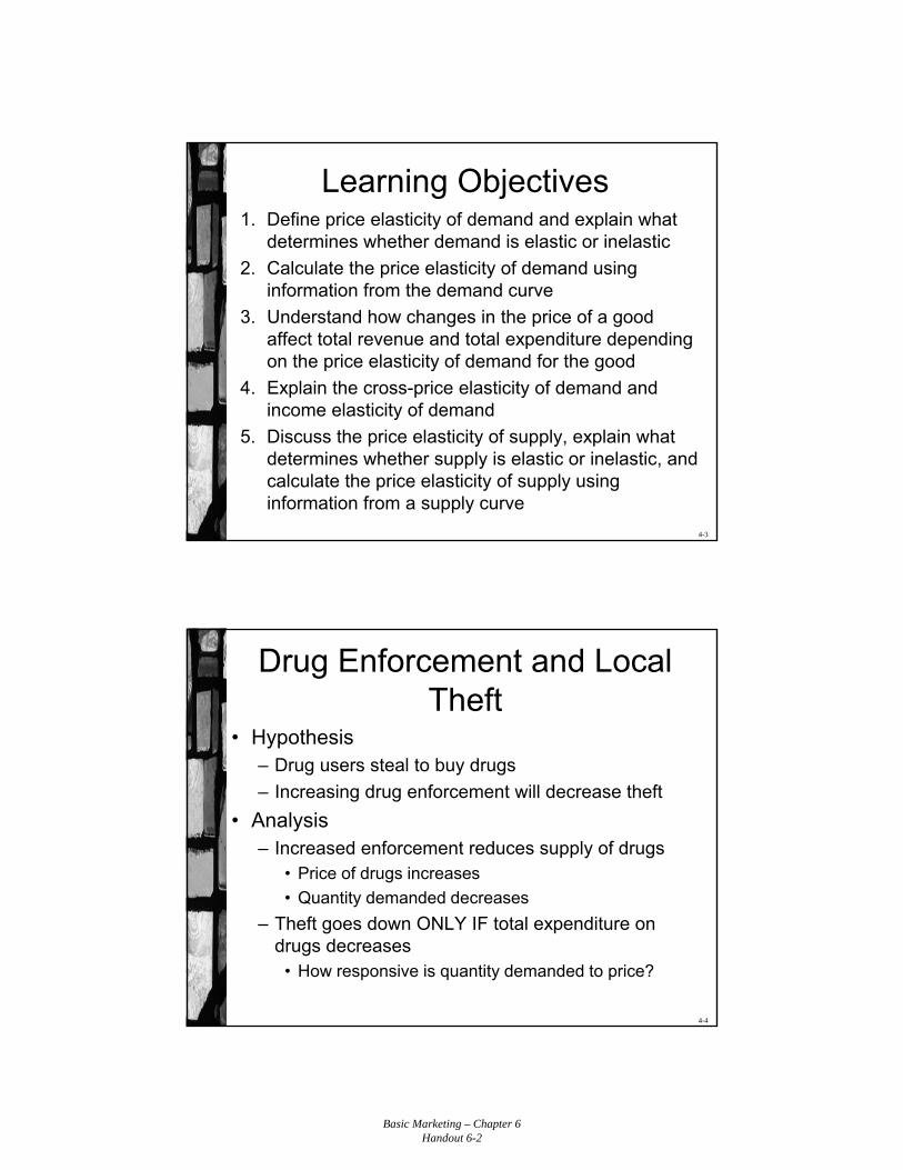
The Basics
MarketsSupply and Demand
Sca
rcity
Cos
t –B
enef
it
Ince
ntiv
e
Com
para
tive
Adv
anta
ge
Incr
easi
ng
Opp
ortu
nity
Cos
ts
Effi
cien
cy
Equ
ilibr
ium
Basic Marketing – Chapter 6Handout 6-2
4-3
Learning Objectives1. Define price elasticity of demand and explain what
determines whether demand is elastic or inelastic
2. Calculate the price elasticity of demand using information from the demand curve
3. Understand how changes in the price of a good affect total revenue and total expenditure depending on the price elasticity of demand for the good
4. Explain the cross-price elasticity of demand and income elasticity of demand
5. Discuss the price elasticity of supply, explain what determines whether supply is elastic or inelastic, and calculate the price elasticity of supply using information from a supply curve
4-4
Drug Enforcement and Local Theft
• Hypothesis– Drug users steal to buy drugs
– Increasing drug enforcement will decrease theft
• Analysis– Increased enforcement reduces supply of drugs
• Price of drugs increases
• Quantity demanded decreases
– Theft goes down ONLY IF total expenditure on drugs decreases
• How responsive is quantity demanded to price?
Basic Marketing – Chapter 6Handout 6-3
4-5
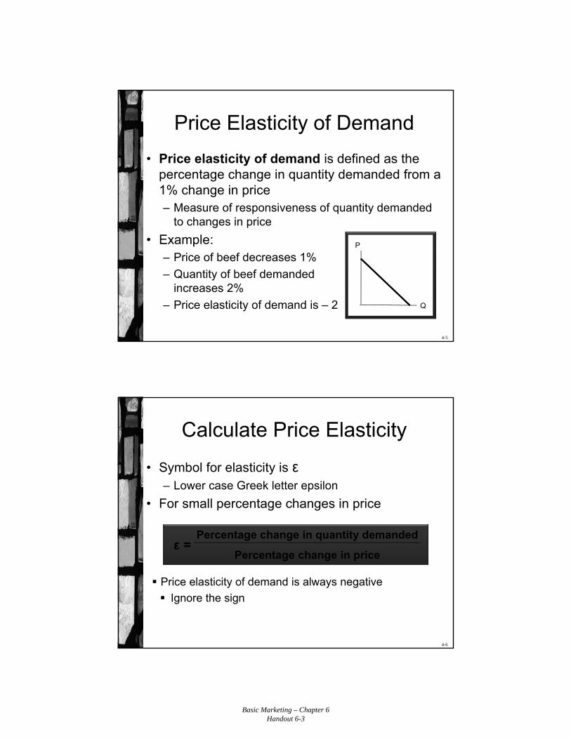
Price Elasticity of Demand
• Price elasticity of demand is defined as the percentage change in quantity demanded from a 1% change in price– Measure of responsiveness of quantity demanded
to changes in price
• Example:– Price of beef decreases 1%
– Quantity of beef demanded increases 2%
– Price elasticity of demand is – 2
P
Q
4-6
Calculate Price Elasticity
• Symbol for elasticity is ε– Lower case Greek letter epsilon
• For small percentage changes in price
ε =Percentage change in quantity demanded
Percentage change in price
Price elasticity of demand is always negative
Ignore the sign
Basic Marketing – Chapter 6Handout 6-4
4-7
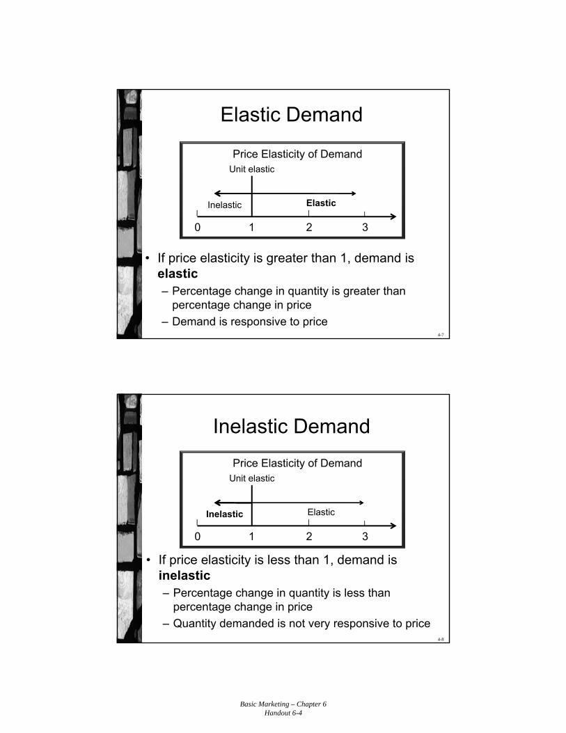
Elastic Demand
• If price elasticity is greater than 1, demand is elastic– Percentage change in quantity is greater than
percentage change in price
– Demand is responsive to price
3
Price Elasticity of Demand
Inelastic
Unit elastic
Elastic
210
4-8
Inelastic Demand
• If price elasticity is less than 1, demand is inelastic– Percentage change in quantity is less than
percentage change in price
– Quantity demanded is not very responsive to price
3
Price Elasticity of Demand
Inelastic
Unit elastic
Elastic
210
Basic Marketing – Chapter 6Handout 6-5
4-9
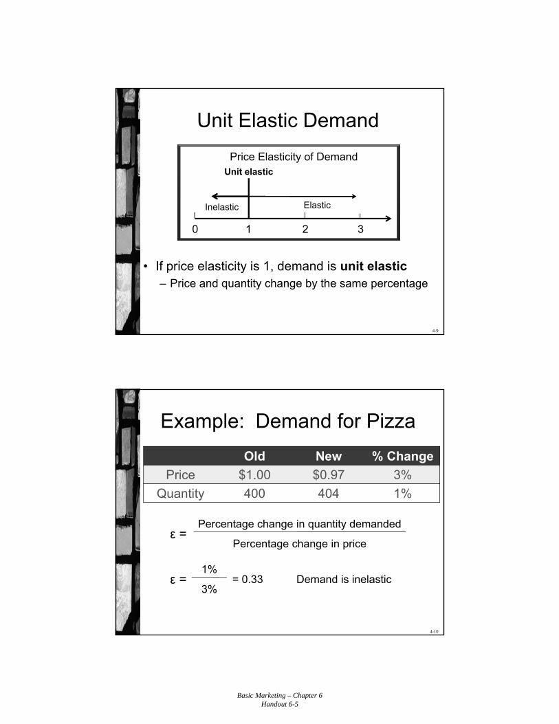
Unit Elastic Demand
• If price elasticity is 1, demand is unit elastic– Price and quantity change by the same percentage
3
Price Elasticity of Demand
Inelastic
Unit elastic
Elastic
210
4-10
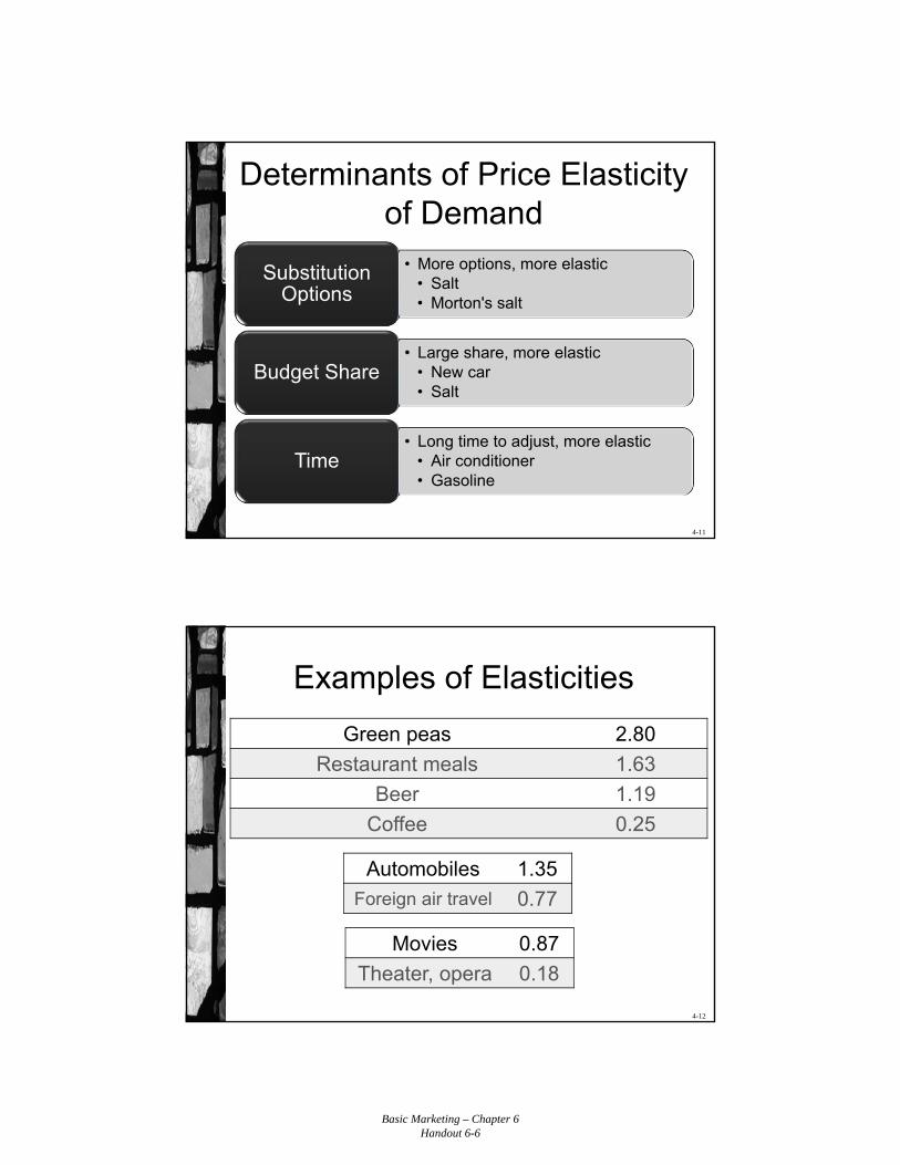
Example: Demand for Pizza
Old New % Change
Price $1.00 $0.97 3%
Quantity 400 404 1%
ε =Percentage change in quantity demanded
Percentage change in price
ε =1%
3%= 0.33 Demand is inelastic
Basic Marketing – Chapter 6Handout 6-6
4-11
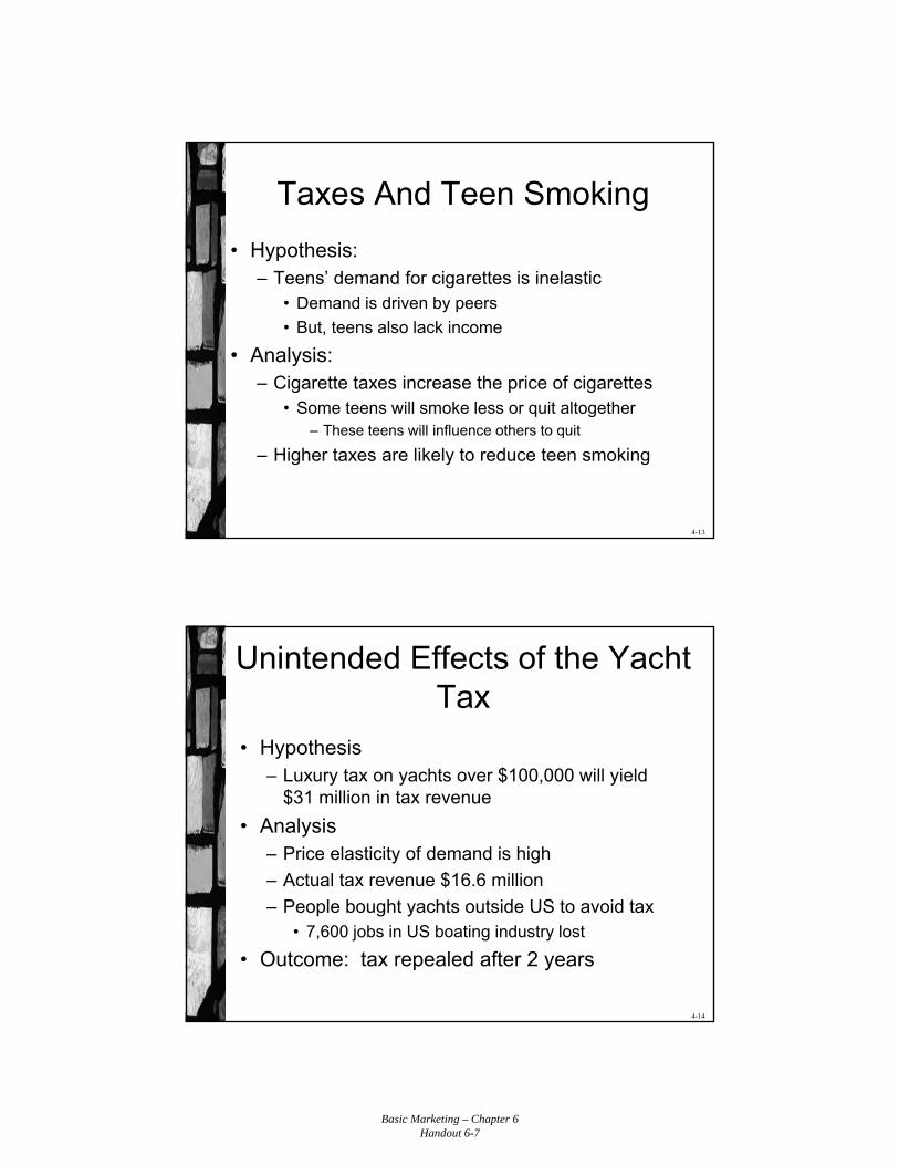
Determinants of Price Elasticity of Demand
• More options, more elastic• Salt• Morton's salt
Substitution Options
• Large share, more elastic• New car• Salt
Budget Share
• Long time to adjust, more elastic• Air conditioner• Gasoline
Time
4-12
Examples of Elasticities
Green peas 2.80
Restaurant meals 1.63
Beer 1.19
Coffee 0.25
Automobiles 1.35
Foreign air travel 0.77
Movies 0.87
Theater, opera 0.18
Basic Marketing – Chapter 6Handout 6-7
4-13
Taxes And Teen Smoking
• Hypothesis:– Teens’ demand for cigarettes is inelastic
• Demand is driven by peers
• But, teens also lack income
• Analysis:– Cigarette taxes increase the price of cigarettes
• Some teens will smoke less or quit altogether– These teens will influence others to quit
– Higher taxes are likely to reduce teen smoking
4-14
Unintended Effects of the Yacht Tax
• Hypothesis– Luxury tax on yachts over $100,000 will yield
$31 million in tax revenue
• Analysis– Price elasticity of demand is high
– Actual tax revenue $16.6 million
– People bought yachts outside US to avoid tax• 7,600 jobs in US boating industry lost
• Outcome: tax repealed after 2 years
Basic Marketing – Chapter 6Handout 6-8
4-15
Price Elasticity Notation
• ∆Q is the change in quantity– ∆Q / Q is percentage change in quantity
• ∆P is change in price– ∆P / P is percentage change in price
ε =Percentage change in quantity demanded
Percentage change in price
ε =∆Q / Q
∆P / P
4-16
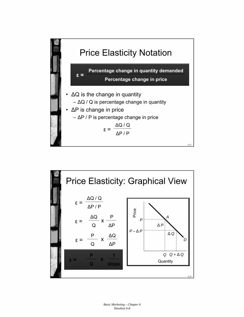
Price Elasticity: Graphical View
ε =∆Q / Q
∆P / P
ε =∆Q
Q
P
∆Px
ε =P
Q
∆Q
∆Px
ε =P
Q
1
slopex
P – ∆ P
Pric
e
P
D
A
Q Q + ∆ Q
∆ Q
∆ P
Quantity
Basic Marketing – Chapter 6Handout 6-9
4-17
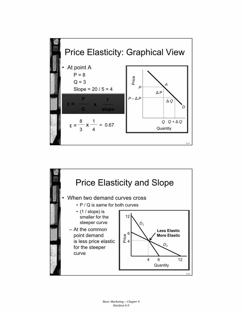
Price Elasticity: Graphical View
• At point AP = 8
Q = 3
Slope = 20 / 5 = 4
ε =8
3
1
4x = 0.67
P – ∆ P
Pric
e
P
D
A
Q Q + ∆ Q
∆ Q
∆ P
Quantity
ε =P
Q slope
1x
4-18
Price Elasticity and Slope
• When two demand curves cross• P / Q is same for both curves
• (1 / slope) is smaller for the steeper curve
– At the common point demand is less price elastic for the steeper curve
D1
D2
12
4 6 12
6
4
Quantity
Pric
e
Less ElasticMore Elastic
Basic Marketing – Chapter 6Handout 6-10
4-19
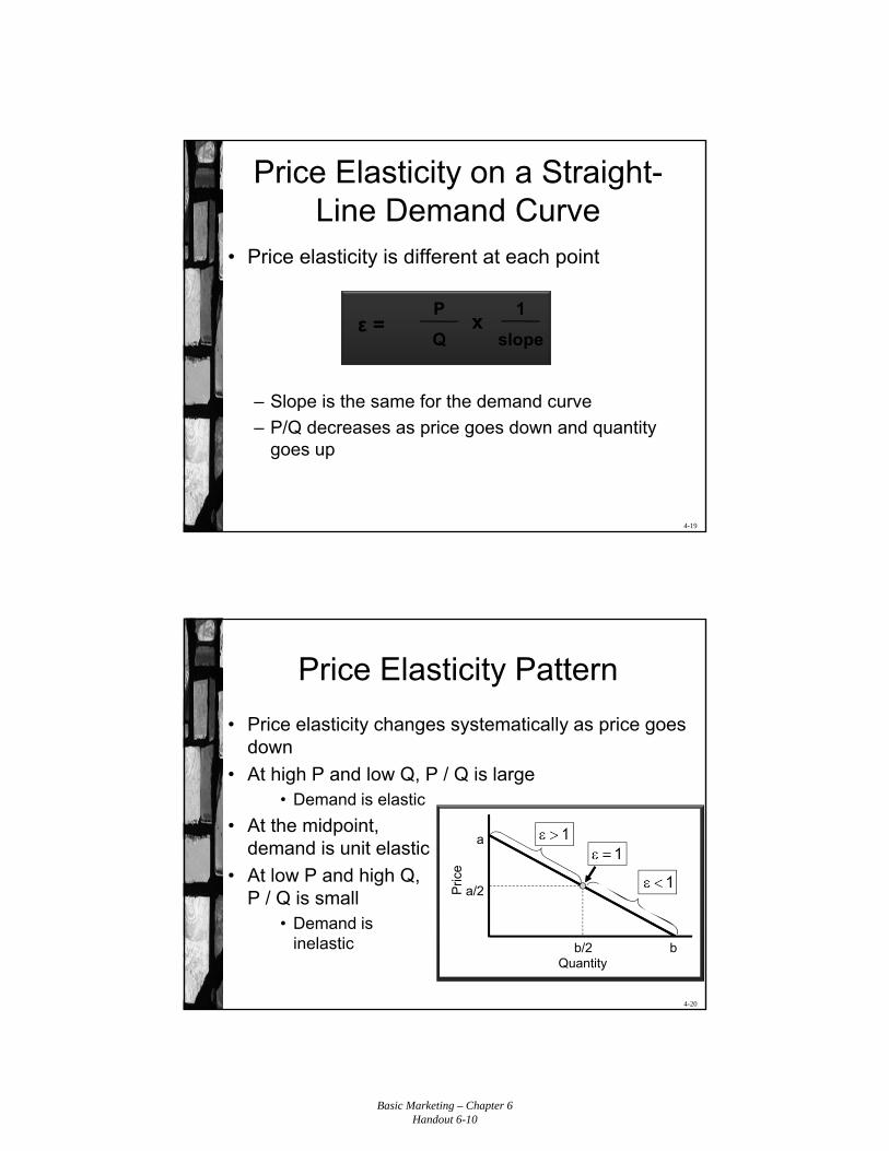
Price Elasticity on a Straight-Line Demand Curve
• Price elasticity is different at each point
– Slope is the same for the demand curve
– P/Q decreases as price goes down and quantity goes up
ε =P
Q
1
slopex
4-20
Price Elasticity Pattern
• Price elasticity changes systematically as price goes down
• At high P and low Q, P / Q is large• Demand is elastic
• At the midpoint, demand is unit elastic
• At low P and high Q, P / Q is small
• Demand is inelastic
Pric
e
b/2
a/2
a
bQuantity
Basic Marketing – Chapter 6Handout 6-11
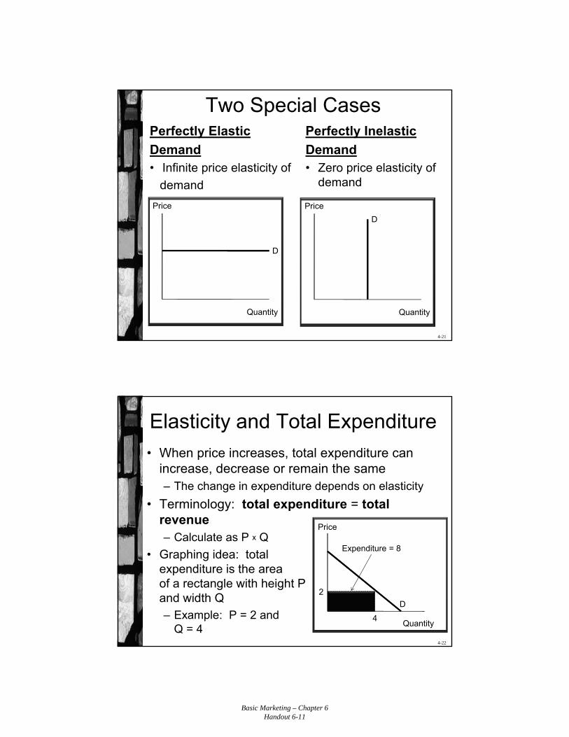
4-21
Two Special CasesPerfectly Elastic
Demand• Infinite price elasticity of
demand
Perfectly Inelastic
Demand• Zero price elasticity of
demand
Price
Quantity
D
Price
Quantity
D
4-22
Elasticity and Total Expenditure
• When price increases, total expenditure can increase, decrease or remain the same– The change in expenditure depends on elasticity
• Terminology: total expenditure = total revenue– Calculate as P x Q
• Graphing idea: total expenditure is the area of a rectangle with height P and width Q– Example: P = 2 and
Q = 4
Price
Quantity
D
2
4
Expenditure = 8
Basic Marketing – Chapter 6Handout 6-12
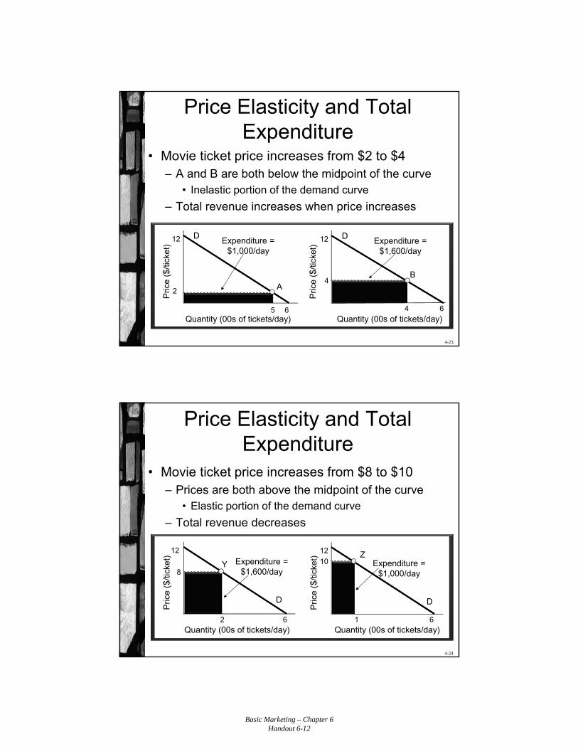
4-23
Price Elasticity and Total Expenditure
• Movie ticket price increases from $2 to $4– A and B are both below the midpoint of the curve
• Inelastic portion of the demand curve
– Total revenue increases when price increases
Quantity (00s of tickets/day)
D
A
Expenditure = $1,000/day
12
Pric
e ($
/tick
et)
5 6
2
Quantity (00s of tickets/day)4
D
B
Expenditure = $1,600/day
12
Pric
e ($
/tick
et)
6
4
4-24
Price Elasticity and Total Expenditure
• Movie ticket price increases from $8 to $10– Prices are both above the midpoint of the curve
• Elastic portion of the demand curve
– Total revenue decreases
D
Expenditure = $1,600/day
12
Quantity (00s of tickets/day)
Pric
e ($
/tick
et)
2 6
8Y
Z
D
Expenditure = $1,000/day
12
Quantity (00s of tickets/day)
Pric
e ($
/tick
et)
1 6
10
Basic Marketing – Chapter 6Handout 6-13
4-25
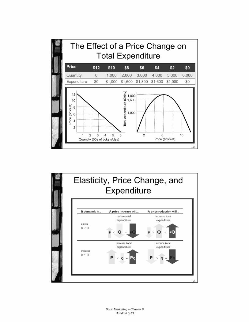
The Effect of a Price Change on Total Expenditure
Price $12 $10 $8 $6 $4 $2 $0
Quantity 0 1,000 2,000 3,000 4,000 5,000 6,000
Expenditure $0 $1,000 $1,600 $1,800 $1,600 $1,000 $0
1,800
Price ($/ticket)
Tota
l exp
endi
ture
($/
day)
2 6 10
1,600
1,000
12
Quantity (00s of tickets/day)
Pric
e ($
/tic
ket)
1 3 4 5 6
10
8
6
4
2
2
4-26
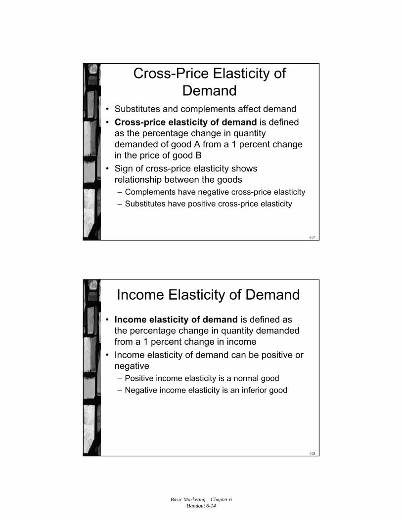
Elasticity, Price Change, and Expenditure
Basic Marketing – Chapter 6Handout 6-14
4-27
Cross-Price Elasticity of Demand
• Substitutes and complements affect demand
• Cross-price elasticity of demand is defined as the percentage change in quantity demanded of good A from a 1 percent change in the price of good B
• Sign of cross-price elasticity shows relationship between the goods– Complements have negative cross-price elasticity
– Substitutes have positive cross-price elasticity
4-28
Income Elasticity of Demand
• Income elasticity of demand is defined as the percentage change in quantity demanded from a 1 percent change in income
• Income elasticity of demand can be positive or negative– Positive income elasticity is a normal good
– Negative income elasticity is an inferior good
Basic Marketing – Chapter 6Handout 6-15
4-29
Price Elasticity of Supply
• Price elasticity of supply – Percentage change in quantity supplied from a
1 percent change in price
Price elasticity of supply =∆Q / Q
∆P / P
Price elasticity of supply =P
Q
1
slopex
4-30
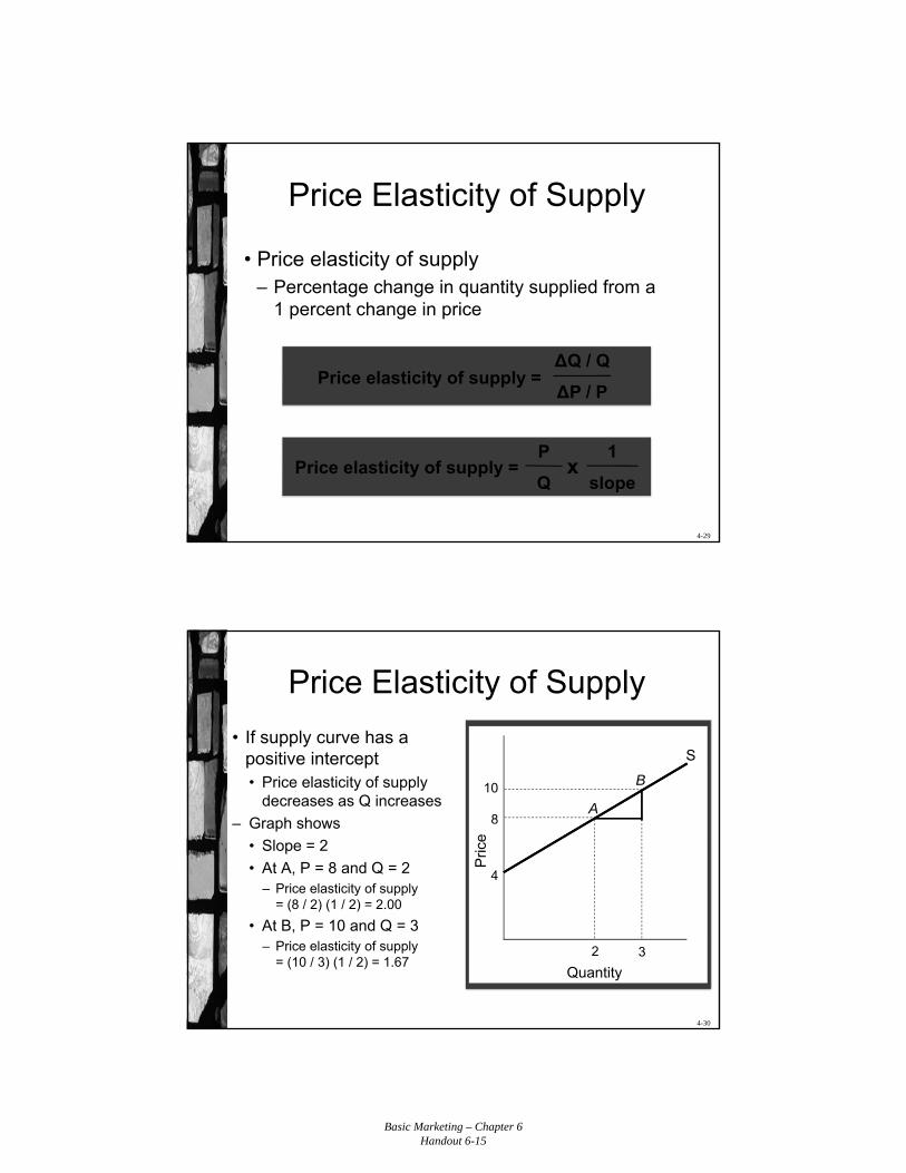
Price Elasticity of Supply
• If supply curve has a positive intercept• Price elasticity of supply
decreases as Q increases
– Graph shows
• Slope = 2
• At A, P = 8 and Q = 2– Price elasticity of supply
= (8 / 2) (1 / 2) = 2.00
• At B, P = 10 and Q = 3– Price elasticity of supply
= (10 / 3) (1 / 2) = 1.672
8A
3
10 B
Quantity
Pric
e
4
S
Basic Marketing – Chapter 6Handout 6-16
4-31
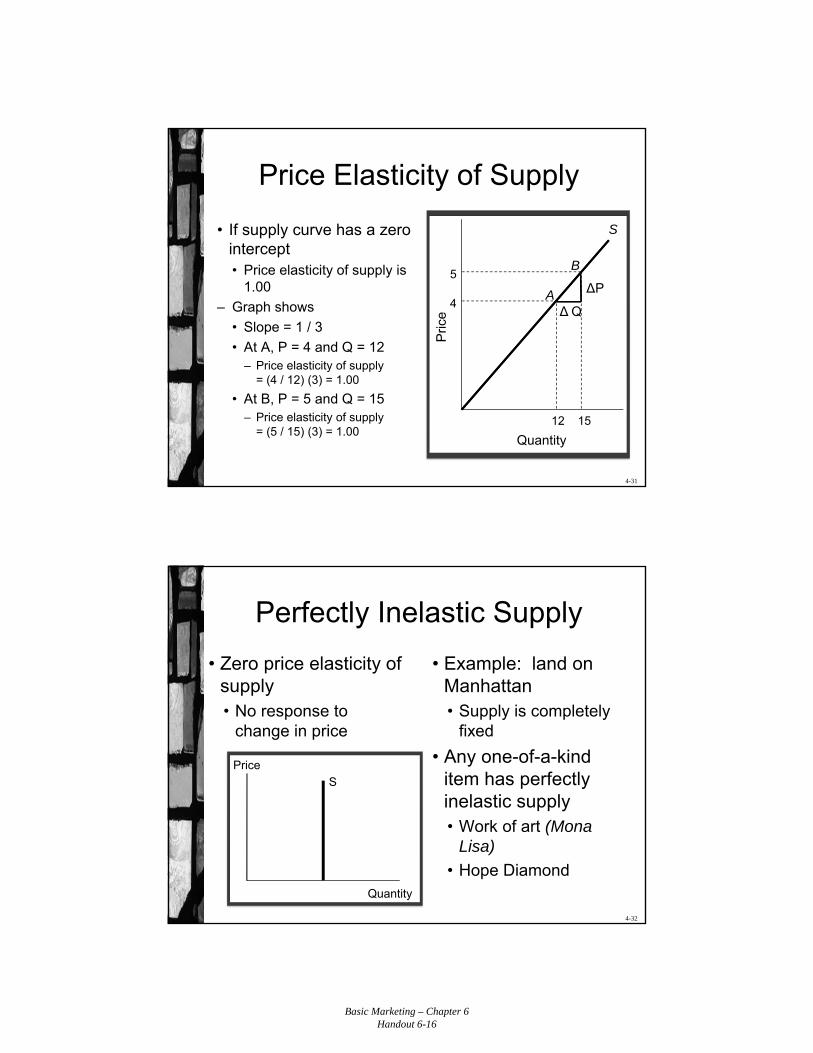
Price Elasticity of Supply
• If supply curve has a zero intercept• Price elasticity of supply is
1.00
– Graph shows
• Slope = 1 / 3
• At A, P = 4 and Q = 12– Price elasticity of supply
= (4 / 12) (3) = 1.00
• At B, P = 5 and Q = 15– Price elasticity of supply
= (5 / 15) (3) = 1.0015
5B
∆P
∆ Q
S
12
4A
QuantityP
rice
4-32
Perfectly Inelastic Supply
• Zero price elasticity of supply• No response to
change in price
• Example: land on Manhattan• Supply is completely
fixed
• Any one-of-a-kind item has perfectly inelastic supply• Work of art (Mona
Lisa)
• Hope Diamond
Price
Quantity
S
Basic Marketing – Chapter 6Handout 6-17
4-33
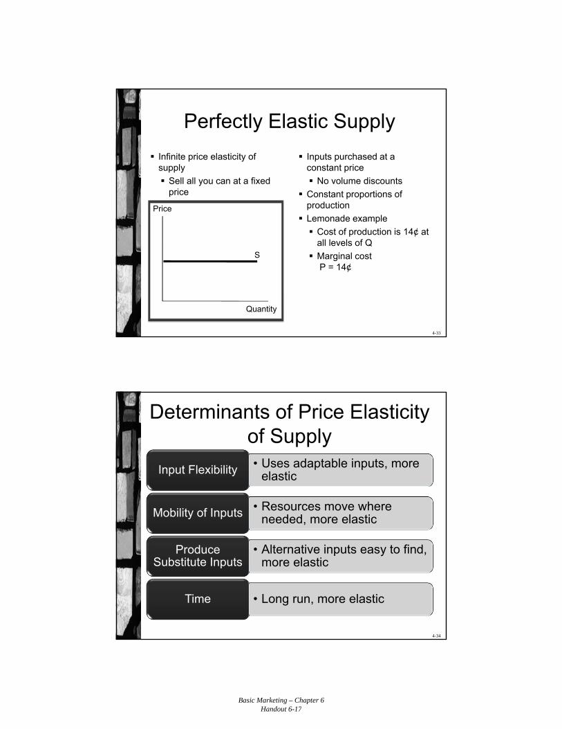
Perfectly Elastic Supply
Infinite price elasticity of supply
Sell all you can at a fixed price
Inputs purchased at a constant price
No volume discounts
Constant proportions of production
Lemonade example
Cost of production is 14¢ at all levels of Q
Marginal cost P = 14¢
Price
Quantity
S
4-34
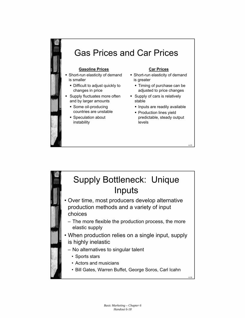
Determinants of Price Elasticity of Supply• Uses adaptable inputs, more
elastic Input Flexibility
• Resources move where needed, more elastic Mobility of Inputs
• Alternative inputs easy to find, more elastic
Produce Substitute Inputs
• Long run, more elasticTime
Basic Marketing – Chapter 6Handout 6-18
4-35
Gas Prices and Car Prices
Gasoline Prices
Short-run elasticity of demand is smaller
Difficult to adjust quickly to changes in price
Supply fluctuates more often and by larger amounts
Some oil-producing countries are unstable
Speculation about instability
Car Prices
Short-run elasticity of demand is greater
Timing of purchase can be adjusted to price changes
Supply of cars is relatively stable
Inputs are readily available
Production lines yield predictable, steady output levels
4-36
Supply Bottleneck: Unique Inputs
• Over time, most producers develop alternative production methods and a variety of input choices– The more flexible the production process, the more
elastic supply
• When production relies on a single input, supply is highly inelastic– No alternatives to singular talent
• Sports stars
• Actors and musicians
• Bill Gates, Warren Buffet, George Soros, Carl Icahn
Basic Marketing – Chapter 6Handout 6-19
4-37
Chapter 4 Appendix
The Midpoint Formula for Demand Elasticity
4-38
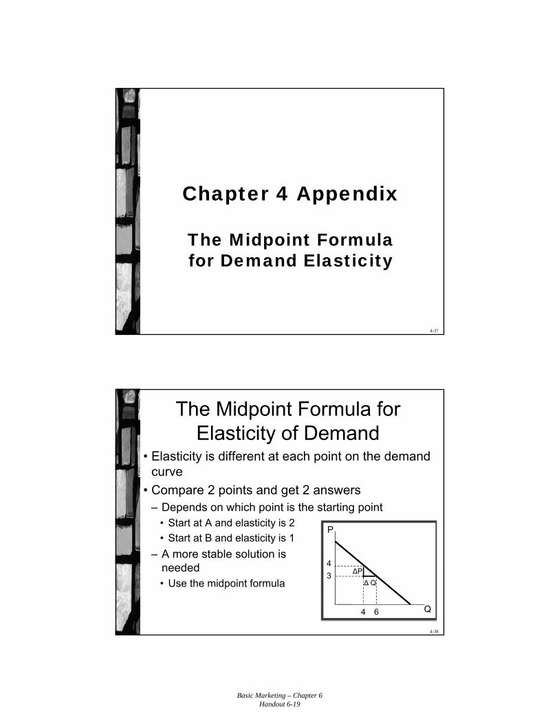
• Elasticity is different at each point on the demand curve
• Compare 2 points and get 2 answers– Depends on which point is the starting point
• Start at A and elasticity is 2
• Start at B and elasticity is 1
– A more stable solution is needed• Use the midpoint formula
The Midpoint Formula for Elasticity of Demand
P
Q
∆P
∆ Q
4
3
4 6
Basic Marketing – Chapter 6Handout 6-20
4-39
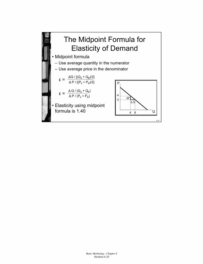
The Midpoint Formula for Elasticity of Demand
• Midpoint formula– Use average quantity in the numerator
– Use average price in the denominator
• Elasticity using midpoint formula is 1.40
∆Q / [(QA + QB)/2]
∆ P / [(PA + PB)/2]ε =
∆ Q / (QA + QB)
∆ P / (PA + PB)ε =
P
Q
∆P
∆ Q
4
3
4 6